A POD-Galerkin reduced order model for Navier-Stokes equations in stream function-vorticity formulation

Abstract.

We develop a Proper Orthogonal Decomposition (POD)-Galerkin based Reduced Order Model (ROM) for the efficient numerical simulation of the parametric Navier-Stokes equations in the stream function-vorticity formulation. Unlike previous works, we choose different reduced coefficients for the vorticity and stream function fields. In addition, for parametric studies we use a global POD basis space obtained from a database of time dependent full order snapshots related to sample points in the parameter space. We test the performance of our ROM strategy with the vortex merger benchmark. Accuracy and efficiency are assessed for both time reconstruction and physical parametrization.

Keywords: Navier-Stokes equations, stream function-vorticity formulation, Proper Orthogonal Decomposition, Reduced order model, Galerkin projection

1. Introduction

The formulation of the 2D Navier–Stokes equations in terms of stream function and vorticity represents an attractive alternative to the model in primitive variables for two main reasons: (i) there are only two scalar unknowns and (ii) the divergence free constraint for the velocity is automatically satisfied by the definition of the stream function. Computational studies on this formulation can be found in, e.g., [4, 21, 23, 36, 40].

While there exists an abundance of literature on Reduced Order Models (ROMs) for the Navier–Stokes equations formulated in primitive variables starting from different Full Order Methods (FOMs), e.g. Finite Element methods [41, 6, 3] or Finite Volume methods [22, 37, 15], it is only relatively recently that ROMs have been applied to the stream function-vorticity formulation [1, 2, 9, 28, 29, 30, 35].

In this paper, we develop a POD–Galerkin ROM for the stream function-vorticity formulation. The main building blocks of our approach are:

• the collection of a database of simulations using a computationally efficient finite volume method;

• the extraction of the most energetic modes representing the system dynamics through Proper Orthogonal Decomposition (POD);

• a Galerkin projection on the space spanned by these most energetic modes for the computation of stream function and vorticity reduced coefficients.

Two are the main novelties of our approach. First, unlike previous works [2, 1, 30, 28, 29, 35] we consider different coefficients for the approximation of the vorticity and stream function fields. This choice leads to two important consequences: (i) the stream function basis functions do not depend on the particular vorticity basis functions, but are instead computed directly from the stream function high-fidelity solutions during the offline phase; (ii) the reduced spaces for the stream function and vorticity can have different dimensions. The second novelty pertains the parametric study with respect to two crucial model parameters (Reynolds number and strength of the forcing term) for which we use a global POD basis space computed by time dependent FOM snapshots associated to sample points in the parameter space. This is a difference with respect to [29, 28, 2, 1, 30], where a POD basis is computed for each parameter in the training set and the the basis functions for new parameter values are found via interpolation of the basis functions associated to the training set.

The work in this paper represents an intermediate step towards the development of new FOM and ROM approaches for the quasi-geostrophic equations that are usually written in terms of stream function and (potential) vorticity. See [25] for a recent review.

All the FOM simulations presented in this work have been performed with OpenFOAM^® [42], an open source Finite Volume C++ library widely used by commercial and academic organizations. For the Navier–Stokes equations in primitive variables, OpenFOAM features several partitioned algorithms (PISO [17], PIMPLE [26] and SIMPLE [27]) based on the Chorin-Temam projection scheme [39]. To the best of our knowledge, no solver for the stream function-vorticity formulation has been shared with the large OpenFOAM^® community. Thus, we have implemented such solver at the FOM level. The ROM computations have been carried out with ITHACA-FV [37], an in-house implementation of several ROM techniques within OpenFOAM^®.

The rest of this paper is organized as follows. In Sec. 2, we describe the full order model and the numerical method we use for its time and space discretization. Sec. 3 presents the reduced order model. The numerical experiments are reported in Sec. 4. Finally, conclusions and future perspectives are provided in Sec. 5.

2. The Full Order Model

2.1. The Navier-Stokes equations in stream function-vorticity formulation

We consider the motion of a two-dimensional incompressible, viscous fluid in a fixed domain $\Omega\subset\mathbb{R}^{2}$ over a time interval of interest $(t_{0},T)$. The flow is described by the incompressible Navier-Stokes equations:

(1) $$\partial_{t}{\mbox{\boldmath{$u$}}}+\nabla\cdot\left({\mbox{\boldmath{$u$}}}\otimes{\mbox{\boldmath{$u$}}}\right)-\dfrac{1}{Re}\Delta{\mbox{\boldmath{$u$}}}+\nabla p ={\mbox{\boldmath{$f$}}}\quad\mbox{ in }\Omega\times(t_{0},T),$$

(2) $$\nabla\cdot{\mbox{\boldmath{$u$}}} =0\quad\,\mbox{ in }\Omega\times(t_{0},T),$$

where eq. (1) states the conservation of linear momentum and eq. (2) represents the conservation of mass. Here, ${\mbox{\boldmath{$u$}}}(x,y,t)=(u(x,y,t),v(x,y,t),0)$ is the fluid velocity, $\partial_{t}$ denotes the time derivative, $p(x,y,t)$ is the pressure and $Re$ is the Reynolds number. In (1), we take into account possible body forces ${\mbox{\boldmath{$f$}}}(x,y,t)$. We focus on forcing terms that can be expressed as product of two functions: one function that depends only on space and the other that depends only on time, i.e. ${\mbox{\boldmath{$f$}}}(x,y,t)=f_{2}(t){\mbox{\boldmath{$f$}}}_{1}(x,y)$. See Remark 3.1 for more details about this choice.

Let $\partial_{x}$ and $\partial_{y}$ denote the derivative with respect to the $x$ and $y$ spatial coordinate, respectively. By applying the curl operator $\nabla\times$ to eq. (1), we obtain the governing equation for the vorticity field $\mbox{\boldmath{$\omega$}}(x,y,t)=\nabla\times{\mbox{\boldmath{$u$}}}=(0,0,\omega)=(0,0,\partial_{x}v-\partial_{y}u)$

$$\partial_{t}\omega+\nabla\cdot\left({\mbox{\boldmath{$u$}}}\omega\right)-\dfrac{1}{Re}\Delta\omega =F\quad\mbox{ in }\Omega\times(t_{0},T),$$

where ${\mbox{\boldmath{$F$}}}=(0,0,F)=\nabla\times{\mbox{\boldmath{$f$}}}$. The incompressibility constraint (2) leads to the introduction of the stream function $\mbox{\boldmath{$\psi$}}(x,y,t)=(0,0,\psi)$ such that ${\mbox{\boldmath{$u$}}}=\nabla\times\mbox{\boldmath{$\psi$}}$, or, equivalently, $(\partial_{y}\psi,-\partial_{x}\psi)=(u,v)$ . The stream function $\psi$ and vorticity $\omega$ are linked by a Poisson equation

$$-\Delta\psi=\omega\quad\mbox{ in }\Omega\times(t_{0},T).$$

To close problem (1)-(2), we need to provide initial data ${\mbox{\boldmath{$u$}}}(x,y,t_{0})={\mbox{\boldmath{$u$}}}_{0}$ and enforce proper boundary conditions. In this work, we consider the following slip condition on the entire boundary:

(3) $${\mbox{\boldmath{$u$}}}\cdot{\mbox{\boldmath{$n$}}} =0\quad\ \mbox{and}\quad\partial_{n}\left({\mbox{\boldmath{$u$}}}\cdot\mbox{\boldmath{$t$}}\right)=0\quad\mbox{ on }\partial\Omega\times(t_{0},T),$$

where $n$ is the outward unit normal and $t$ the unit tangent vector to $\partial\Omega$. In terms of $\psi$ and $\omega$, we consider initial data $\omega(x,y,t_{0})=\omega_{0}$ and express (3) as $\psi=\partial_{n}\omega=0$.

Summarizing, the Navier-Stokes equations in stream function-vorticity formulation, which represent our full order model, are given by

(4) $$\partial_{t}\omega+\nabla\cdot\left(\left(\nabla\times\mbox{\boldmath{$\psi$}}\right)\omega\right)-\dfrac{1}{Re}\Delta\omega =F\quad\mbox{ in }\Omega\times(t_{0},T),$$

(5) $$-\Delta\psi =\omega\quad\mbox{ in }\Omega\times(t_{0},T),$$

endowed with boundary conditions

(6) $$\psi =0\quad\ \mbox{ on }\partial\Omega\times(t_{0},T),$$

(7) $$\partial_{n}\omega =0\quad\ \mbox{ on }\partial\Omega\times(t_{0},T),$$

and initial data $\omega(x,y,t_{0})=\omega_{0}$.

2.2. Time and space discretization

Let us start with the time discretization of the FOM (4)-(5). Let $\Delta t\in\mathbb{R}$, $t^{n}=t_{0}+n\Delta t$, with $n=0,...,N_{T}$ and $T=t_{0}+N_{T}\Delta t$. We denote by $y^{n}$ the approximation of a generic quantity $y$ at the time $t^{n}$. Problem (4)-(5) discretized in time by a Backward Differentiation Formula of order 1 (BDF1) reads: given $\omega^{0}=\omega_{0}$, for $n\geq 0$ find the solution $(\psi^{n+1},\omega^{n+1})$ of system:

(8) $$\frac{1}{\Delta t}\,\omega^{n+1}+\nabla\cdot\left(\left(\nabla\times\mbox{\boldmath{$\psi$}}^{n+1}\right)\omega^{n+1}\right)-\dfrac{1}{Re}\Delta\omega^{n+1} =b^{n+1},$$

(9) $$\nabla\psi^{n+1} =\omega^{n+1},$$

where $b^{n+1}=F^{n+1}+\omega^{n}/\Delta t$. In order to contain the computational cost required to approximate the solution to problem (8)-(9), we opt for a segregated algorithm. Given the vorticity $\omega^{n}$, at $t^{n+1}$ such algorithm requires to:

• Find the vorticity $\omega^{n+1}$ such that

  (10) $$\frac{1}{\Delta t}\,\omega^{n+1}+\nabla\cdot\left(\left(\nabla\times\mbox{\boldmath{$\psi$}}^{*}\right)\omega^{n+1}\right)-\dfrac{1}{Re}\Delta\omega^{n+1} =b^{n+1},$$

  where $\mbox{\boldmath{$\psi$}}^{n+1}$ in (8) is replaced by an extrapolation $\mbox{\boldmath{$\psi$}}^{*}$. Since we are using BDF1, we set $\mbox{\boldmath{$\psi$}}^{*}=\mbox{\boldmath{$\psi$}}^{n}$.

• Find $\psi^{n+1}$ such that

  (11) $$\nabla\psi^{n+1}=-\omega^{n+1}.$$

For the space discretization of problem (10)-(11), we adopt a Finite Volume (FV) approximation that is derived directly from the integral form of the governing equations. For this purpose, we partition the computational domain $\Omega$ into cells or control volumes $\Omega_{i}$, with $i=1,\dots,N_{c}$, where $N_{c}$ is the total number of cells in the mesh. The integral form of eq. (10) for each volume $\Omega_{i}$ is given by:

$$\frac{1}{\Delta t}\,\int_{\Omega_{i}}\omega^{n+1}d\Omega +\int_{\Omega_{i}}\nabla\cdot\left(\left(\nabla\times\mbox{\boldmath{$\psi$}}^{n}\right)\omega^{n+1}\right)d\Omega$$

(12) $$-\dfrac{1}{Re}\int_{\Omega_{i}}\Delta\omega^{n+1}d\Omega=\int_{\Omega_{i}}b^{n+1}d\Omega.$$

By applying the Gauss-divergence theorem, eq. (2.2) becomes:

$$\frac{1}{\Delta t}\,\int_{\Omega_{i}}\omega^{n+1}d\Omega +\int_{\partial\Omega_{i}}\left(\left(\nabla\times\mbox{\boldmath{$\psi$}}^{n}\right)\omega^{n+1}\right)\cdot d\textbf{A}$$

(13) $$-\dfrac{1}{Re}\int_{\partial\Omega_{i}}\nabla\omega^{n+1}\cdot d\textbf{A}=\int_{\Omega_{i}}b^{n+1}d\Omega,$$

where A is the surface vector associated with the boundary of $\Omega_{i}$.

Let A_j be the surface vector of each face of the control volume, with $j=1,\dots,M$. Each term in eq. (2.2) is approximated as follows:

• Convective term:

  (14) $$\int_{\partial\Omega_{i}}\left(\left(\nabla\times\mbox{\boldmath{$\psi$}}^{n}\right)\omega^{n+1}\right)\cdot d\textbf{A} \approx\sum_{j}\left(\left(\nabla\times\mbox{\boldmath{$\psi$}}_{j}^{n}\right)\omega^{n+1}_{j}\right)\cdot\textbf{A}_{j}=\sum_{j}\varphi_{j}^{n}\omega^{n+1}_{j},$$

  (15) $$\varphi_{j}^{n} =\left(\nabla\times\mbox{\boldmath{$\psi$}}_{j}^{n}\right)\cdot\textbf{A}_{j}.$$

  In (14), $\nabla\times\mbox{\boldmath{$\psi$}}_{j}^{n}$ is the extrapolated convective velocity and $\omega^{n+1}_{j}$ is the vorticity, both relative to the centroid of each control volume face. In (15), $\varphi_{j}^{n}$ is the convective flux associated to $\nabla\times\mbox{\boldmath{$\psi$}}^{n}$ through face $j$ of the control volume. In OpenFOAM^® solvers, the convective flux at the cell faces is typically a linear interpolation of the values from the adjacent cells. We also need to approximate $\omega^{n+1}$ at cell face $j$. Different interpolation methods can be applied, including central, upwind, second order upwind, and blended differencing schemes [18]. In this work, we use a Central Differencing (CD) scheme.

• Diffusion term:

  $$\int_{\partial\Omega_{i}}\nabla\omega^{n+1}\cdot d\textbf{A}\approx\sum_{j}(\nabla\omega^{n+1})_{j}\cdot\textbf{A}_{j},$$

  where $(\nabla\omega^{n+1})_{j}$ is the gradient of $\omega^{n+1}$ at face $j$. Let us briefly explain how $(\nabla\omega^{n+1})_{j}$ is approximated with second order accuracy on a structured, orthogonal mesh. Let $P$ and $Q$ be two neighboring control volumes (see Fig. 1).

  

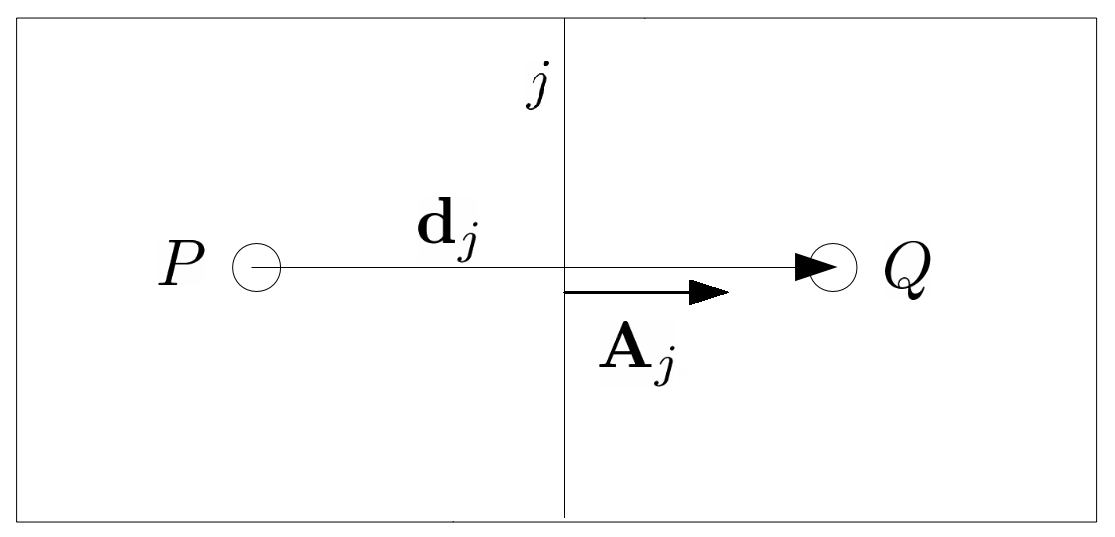
  Figure 1. Close-up view of two orthogonal control volumes in a 2D configuration.

  The term $(\nabla\omega^{n+1})_{j}$ is evaluated by subtracting the value of vorticity at the cell centroid on the $P$-side of the face (denoted with $\omega^{n+1}_{P}$) from the value of vorticity at the centroid on the $Q$-side (denoted with $\omega^{n+1}_{Q}$) and dividing by the magnitude of the distance vector $\textbf{d}_{j}$ connecting the two cell centroids:

  $$(\nabla\omega^{n+1})_{j}\cdot\textbf{A}_{j}=\dfrac{\omega^{n+1}_{Q}-\omega^{n+1}_{P}}{|\textbf{d}_{j}|}|\textbf{A}_{j}|.$$

Let us denote with $\omega^{n+1}_{i}$ and $b^{n+1}_{i}$ the average vorticity and source term in control volume $\Omega_{i}$, respectively. Moreover, we denote with $\omega^{n+1}_{i,j}$ the vorticity associated to the centroid of face $j$ normalized by the volume of $\Omega_{i}$. Then, the discretized form of eq. (2.2), divided by the control volume $\Omega_{i}$, can be written as:

(16) $$\frac{1}{\Delta t}\,\omega^{n+1}_{i} +\sum_{j}\varphi^{n}_{j}\omega^{n+1}_{i,j}-\dfrac{1}{Re}\sum_{j}(\nabla\omega^{n+1}_{i})_{j}\cdot\textbf{A}_{j}=b^{n+1}_{i}.$$

Next, we deal with the space approximation of the eq. (11). After using Gauss-divergence theorem, the integral form of eq. (11) reads:

(17) $$-\int_{\partial\Omega_{i}}\nabla\psi^{n+1}\cdot d\textbf{A}=\int_{\Omega_{i}}{\omega}^{n+1}d\Omega.$$

Once we approximate the integrals and divide by the control volume $\Omega_{i}$, eq. (17) becomes:

(18) $$-\sum_{j}(\nabla\psi^{n+1}_{i})_{j}\cdot\textbf{A}_{j}=\omega^{n+1}_{i}.$$

In eq. (18), $(\nabla\psi^{n+1}_{i})_{j}$ is the gradient of $\psi^{n+1}$ at faces $j$ and it is approximated in the same way as $(\nabla\omega^{n+1}_{i})_{j}$. Finally, the fully discretized form of problem (10)-(11) is given by system (16), (18).

As mentioned in Sec. 1, for the implementation of the numerical scheme described in this section we chose the finite volume C++ library OpenFOAM^® [42].

3. The Reduced Order Model

The main idea of reduced order modeling for parametrized PDEs is the assumption that solutions live in a low dimensional manifold. Thus, any solution can be approximated as a linear combination of a reduced number of global basis functions.

We approximate vorticity field $\omega$ and stream function $\psi$ as linear combinations of the dominant modes (basis functions), which are assumed to be dependent on space variables only, multiplied by scalar coefficients that depend on time and/or parameters. We arrange all the parameters the problem depends upon in a vector $\pi$ that belongs to a $d$-dimensional parameter space $\mathcal{P}$ in $\mathbb{R}^{d}$, where $d$ is the number of parameters. Thus, we have:

(19) $$\omega\approx\omega_{r}=\sum_{i=1}^{N_{\omega}^{r}}\beta_{i}(\mbox{\boldmath{$\pi$}},t){\varphi}_{i}(\mbox{\boldmath{$x$}}),\quad\psi\approx\psi_{r}=\sum_{i=1}^{N_{\psi}^{r}}\gamma_{i}(\mbox{\boldmath{$\pi$}},t)\xi_{i}(\mbox{\boldmath{$x$}}).$$

In (19), $N_{\Phi}^{r}$, $\Phi=\omega,\psi$, denotes the cardinality of a reduced basis for the space field $\Phi$ belongs to. We remark that we consider different coefficients for the approximation of the vorticity $\omega$ and stream function $\psi$ fields, unlike previous works [1, 2, 28, 29, 30, 35]. This choice will be justified numerically in Sec. 4.2.

Remark 3.1.

As mentioned earlier, we only consider a body force given by the product between a space dependent function and a time dependent function. For the stream function-vorticity formulation, this means:

$$F(x,y,z)=F_{2}(t)F_{1}(x,y).$$

Thanks to this assumption, the forcing term is already expressed in the form of (19) and does not require further treatment.

Using (19) to approximate $\omega^{n+1}$ and $\psi^{n+1}$ in (10)-(11), we obtain

(20) $$\frac{1}{\Delta t}\,\omega_{r}^{n+1}+\nabla\cdot\left(\left(\nabla\times\mbox{\boldmath{$\psi$}}_{r}^{*}\right)\omega_{r}^{n+1}\right)-\dfrac{1}{Re}\Delta\omega_{r}^{n+1} =b_{r}^{n+1},$$

(21) $$\nabla\psi_{r}^{n+1} =-\omega_{r}^{n+1},$$

where $b_{r}^{n+1}=F^{n+1}+\omega_{r}^{n}/\Delta t$ and we set $\mbox{\boldmath{$\psi$}}_{r}^{*}=\mbox{\boldmath{$\psi$}}_{r}^{n}$.

In the literature, one can find several techniques to generate the reduced basis spaces, e.g., Proper Orthogonal Decomposition (POD), the Proper Generalized Decomposition and the Reduced Basis with a greedy sampling strategy. See, e.g., [5, 7, 8, 10, 19, 31, 33]. We generate the reduced basis spaces with the method of snapshots. Next, we briefly describe how this method works.

Let $\mathcal{K}=\{\mbox{\boldmath{$\pi$}}^{1},\dots,\mbox{\boldmath{$\pi$}}^{N_{k}}\}$ be a finite dimensional training set of samples chosen inside the parameter space $\mathcal{P}$. We solve the FOM described in Sec. 2 for each $\mbox{\boldmath{$\pi$}}^{k}\in\mathcal{K}$ and for each time instant $t^{j}\in\{t^{1},\dots,t^{N_{t}}\}\subset(t_{0},T]$. The snapshots matrices are obtained from the full-order snapshots:

(22) $$\mbox{\boldmath{$\mathcal{S}$}}_{{{\Phi}}}=[{{\Phi}}(\mbox{\boldmath{$\pi$}}^{1},t^{1}),\dots,{{\Phi}}(\mbox{\boldmath{$\pi$}}^{N_{k}},t^{N_{t}})]\in\mathbb{R}^{N_{\Phi}^{h}\times N_{s}}\quad\text{for}\quad{{\Phi}}=\{\omega_{h},\psi_{h}\},$$

where $N_{s}=N_{t}\cdot N_{k}$ is the total number of the snapshots, $N_{\Phi}^{h}$ is the dimension of the space $\Phi$ belong to in the FOM, and the subscript $h$ indicates a solution computed with the FOM. The POD problem consists in finding, for each value of the dimension of the POD space $N_{POD}=1,\dots,N_{s}$, the scalar coefficients $a_{1}^{1},\dots,a_{1}^{N_{s}},\dots,a_{N_{s}}^{1},\dots,a_{N_{s}}^{N_{s}}$ and functions ${\zeta}_{1},\dots,{\zeta}_{N_{s}}$, that minimize the error between the snapshots and their projection onto the POD basis. In the $L^{2}$-norm, we have

$$E_{N_{POD}}=\text{arg min}\sum_{i=1}^{N_{s}}||{{\Phi}_{i}}-\sum_{k=1}^{N_{POD}}a_{i}^{k}{\zeta}_{k}||\quad\forall N_{POD}=1,\dots,N_{s}$$

(23) $$\text{with}\quad({\zeta}_{i},{\zeta}_{j})_{L_{2}(\Omega)}=\delta_{i,j}\quad\forall i,j=1,\dots,N_{s}.$$

It can be shown [20] that problem (23) is equivalent to the following eigenvalue problem

(24) $$\mbox{\boldmath{$\mathcal{C}$}}^{{\Phi}}\mbox{\boldmath{$Q$}}^{{\Phi}} =\mbox{\boldmath{$Q$}}^{{\Phi}}\mbox{\boldmath{$\Lambda$}}^{{\Phi}},$$

(25) $$\mathcal{C}_{ij}^{\Phi} =({\Phi}_{i},{\Phi}_{j})_{L_{2}(\Omega)}\quad\text{for}\quad i,j=1,\dots,N_{s},$$

where $\mbox{\boldmath{$\mathcal{C}$}}^{{\Phi}}$ is the correlation matrix computed from the snapshot matrix $\mbox{\boldmath{$\mathcal{S}$}}_{{{\Phi}}}$, $\mbox{\boldmath{$Q$}}^{{\Phi}}$ is the matrix of eigenvectors and $\mbox{\boldmath{$\Lambda$}}^{{\Phi}}$ is a diagonal matrix whose diagonal entries are the eigenvalues of $\mbox{\boldmath{$\mathcal{C}$}}^{{\Phi}}$. Then, the basis functions are obtained as follows:

(26) $${\zeta}_{i}=\dfrac{1}{N_{s}\Lambda_{i}^{\Phi}}\sum_{j=1}^{N_{s}}{\Phi}_{j}Q_{ij}^{\Phi}.$$

The POD modes resulting from the aforementioned methodology are:

(27) $$L_{\Phi}=[{\zeta}_{1},\dots,{\zeta}_{N_{\Phi}^{r}}]\in\mathbb{R}^{N_{\Phi}^{h}\times N_{\Phi}^{r}},$$

where the values of $N_{\Phi}^{r}<N_{s}$ are chosen according to the eigenvalue decay of the vectors of eigenvalues $\Lambda$. Then, the reduced order model can be obtained through a Galerkin projection of the governing equations onto the POD spaces.

In order to write the algebraic system associated with the reduced problem (20)-(21), we introduce the following matrices:

(28) $$M_{r_{ij}}=({\varphi}_{i},{\varphi}_{j})_{L_{2}(\Omega)},\quad\widetilde{M}_{r_{ij}}=({\xi}_{i},{\varphi}_{j})_{L_{2}(\Omega)},\quad A_{r_{ij}}=({\varphi}_{i},\Delta{\varphi}_{j})_{L_{2}(\Omega)},$$

(29) $$B_{r_{ij}}=({\xi}_{i},\Delta\xi_{j})_{L_{2}(\Omega)},\quad G_{r_{ijk}}=(\varphi_{i},\nabla\cdot\left(\left(\nabla\times\xi_{j}\right)\varphi_{k}\right))_{L_{2}(\Omega)},$$

(30) $$H_{r_{ij}}=({\varphi}_{i},F_{1})_{L_{2}(\Omega)},$$

where ${\varphi}_{i}$ and $\xi_{i}$ are the basis functions in (19). At time $t^{n+1}$, the reduced algebraic system for (20)-(21) reads: given $\mbox{\boldmath{$\beta$}}^{n}$ and $\mbox{\boldmath{$\gamma$}}^{n}$ find vectors $\mbox{\boldmath{$\beta$}}^{n+1}$ and $\mbox{\boldmath{$\gamma$}}^{n+1}$ containing the values of coefficients $\beta_{i}$ and $\gamma_{i}$ in (19) at time $t^{n+1}$ such that

(31) $$\mbox{\boldmath{$M$}}_{r}\left(\dfrac{\mbox{\boldmath{$\beta$}}^{n+1}-\mbox{\boldmath{$\beta$}}^{n}}{\Delta t}\right)+\left(\mbox{\boldmath{$\gamma$}}^{n}\right)^{T}\mbox{\boldmath{$G$}}_{r}\mbox{\boldmath{$\beta$}}^{n+1}-\dfrac{1}{Re}\mbox{\boldmath{$A$}}_{r}\mbox{\boldmath{$\beta$}}^{n+1}=\mbox{\boldmath{$H$}}_{r}F_{2}^{n+1},$$

(32) $$\mbox{\boldmath{$B$}}_{r}\mbox{\boldmath{$\gamma$}}^{n+1}+\widetilde{\mbox{\boldmath{$M$}}_{r}}\mbox{\boldmath{$\beta$}}^{n+1}=0.$$

Finally, the initial conditions for the ROM algebraic system (31)-(32) are obtained performing a Galerkin projection of the initial full order condition onto the POD basis spaces:

(33) $${\beta^{0}}_{i}=(\omega_{0},{\varphi}_{i})_{L_{2}(\Omega)}.$$

Remark 3.2.

We consider homogeneous boundary conditions (6)-(7). So, the approximated vorticity $\omega_{r}$ and stream function $\psi_{r}$ automatically satisfy the boundary conditions and no special treatment (such as lifting function and penalty methods [15, 22, 37, 38]) is necessary.

4. Numerical results

In order to validate our FOM and ROM approaches, we consider a widely used benchmark test known as the vortex merger. It consists in fluid motion induced by a pair of co-rotating vortices separated from each other by a certain distance. One of the reasons why this test has been extensively investigated in two-dimensions is that it explains the average inverse energy and direct enstrophy cascades observed in two-dimensional turbulence [32].

The computational domain is a $2\pi\times 2\pi$ rectangle. The initial condition for the vortex merger test case is given by:

(34) $$\omega(x,y,0)=\omega_{0}(x,y)=e^{\left(-\pi\left[\left(x-x_{1}\right)^{2}+\left(y-y_{1}\right)^{2}\right]\right)}+e^{\left(-\pi\left[\left(x-x_{2}\right)^{2}+\left(y-y_{2}\right)^{2}\right]\right)},$$

where ($x_{1}$, $y_{1}$) and ($x_{2}$, $y_{2}$) are the initial locations of the centers of the vortices. We set them as ($3\pi/4$, $\pi$) and ($5\pi/4$, $\pi$), respectively. Fig. 2 shows the initial vorticity $\omega_{0}$ (left) and corresponding initial velocity ${\mbox{\boldmath{$u$}}}_{0}$ (right). We note that the initial condition ${\mbox{\boldmath{$u$}}}_{0}(x,y)={\mbox{\boldmath{$u$}}}(x,y,0)=\nabla\times\mbox{\boldmath{$\psi$}}_{0}$ is computed by solving $\Delta\psi_{0}=\omega_{0}$. We let the system evolve until time $T=20$. As previously mentioned, we enforce boundary conditions (6)-(7).

Following [1, 2, 28, 29, 30], we consider a computational grid with $256^{2}=65536$ cells for all the simulations whose results are reported next.

\begin{overpic}[width=147.4292pt]{img/omega0.png} \end{overpic}

\begin{overpic}[width=147.4292pt]{img/U0.png} \end{overpic}

Figure 2. Initial conditions for $\omega_{0}$ (left) and ${\mbox{\boldmath{$u$}}}_{0}$ (right).

4.1. Validation of the FOM

Let us start with the validation of our implementation of the stream function-vorticity formulation at the FOM level. We compare the results obtained with such formulation against the results produced by the standard Navier–Stokes solver in OpenFOAM icoFoam, which is based on a partitioned algorithm called PISO [17]. We set $\Delta t=0.01$, ${\mbox{\boldmath{$f$}}}={\mbox{\boldmath{$F$}}}=0$ and $Re=800$ [28, 29]. For the simulations with icoFoam, we enforce boundary condition (3). The partitioned algorithm requires also a boundary condition for the pressure problem: we set $\nabla p\cdot{\mbox{\boldmath{$n$}}}=0$ on $\partial\Omega$.

Figures 3, 4, and 5 display a qualitative comparison in terms of $u$, $\psi$, and $\omega$ computed by the solvers in primitive variables and in stream function-vorticity formulation at four different times. As we can see from these figures, the solutions are very close to each other with the maximum relative difference in absolute value not exceeding $4.4e-3$ for $u$, $2.5e-3$ for $\psi$, and $6.8e-3$ for $\omega$.

\begin{overpic}[width=86.72267pt,grid=false]{img/U_uvp_4.png} \put(38.0,101.0){$t=4$} \put(-30.0,50.0){NSE} \put(-28.0,40.0){${\mbox{\boldmath{$u$}}},p$} \end{overpic}

\begin{overpic}[width=86.72267pt]{img/U_uvp_8.png} \put(38.0,101.0){$t=8$} \end{overpic}

\begin{overpic}[width=86.72267pt]{img/U_uvp_16.png} \put(35.0,101.0){$t=16$} \end{overpic}

\begin{overpic}[width=86.72267pt]{img/U_uvp_20.png} \put(35.0,101.0){$t=20$} \end{overpic}

\begin{overpic}[width=39.0242pt,grid=false]{img/legendUFOM.png} \end{overpic}

\begin{overpic}[width=86.72267pt]{img/U_psiomega_4.png} \put(-30.0,50.0){NSE} \put(-28.0,40.0){$\psi,\omega$} \end{overpic}

\begin{overpic}[width=86.72267pt]{img/U_psiomega_8.png} \end{overpic}

\begin{overpic}[width=86.72267pt]{img/U_psiomega_16.png} \end{overpic}

\begin{overpic}[width=86.72267pt]{img/U_psiomega_20.png} \end{overpic}

\begin{overpic}[width=39.0242pt]{img/legendUFOM.png} \end{overpic}

\begin{overpic}[width=86.72267pt]{img/U_err_4.png} \put(-30.0,50.0){Diff.} \end{overpic}

\begin{overpic}[width=86.72267pt]{img/U_err_8.png} \end{overpic}

\begin{overpic}[width=86.72267pt]{img/U_err_16.png} \end{overpic}

\begin{overpic}[width=86.72267pt]{img/U_err_20.png} \end{overpic}

\begin{overpic}[width=39.0242pt]{img/legendUerrFOM.png} \end{overpic}

Figure 3. FOM validation: velocity $u$ computed by the solver in velocity-pressure formulation (first row) and stream function-vorticity formulation (second row), and difference between the two fields in absolute value (third row) at $t=4$ (first column), $t=8$ (second column), $t=16$ (third column) and $t=20$ (fourth column).

\begin{overpic}[width=86.72267pt]{img/psi_uvp_4.png} \put(38.0,101.0){$t=4$} \put(-30.0,50.0){NSE} \put(-28.0,40.0){${\mbox{\boldmath{$u$}}},p$} \end{overpic}

\begin{overpic}[width=86.72267pt]{img/psi_uvp_8.png} \put(38.0,101.0){$t=8$} \end{overpic}

\begin{overpic}[width=86.72267pt]{img/psi_uvp_16.png} \put(35.0,101.0){$t=16$} \end{overpic}

\begin{overpic}[width=86.72267pt]{img/psi_uvp_20.png} \put(35.0,101.0){$t=20$} \end{overpic}

\begin{overpic}[width=34.69038pt]{img/legendPsiFOM.png} \end{overpic}

\begin{overpic}[width=86.72267pt]{img/psi_psiomega_4.png} \put(-30.0,50.0){NSE} \put(-28.0,40.0){$\psi,\omega$} \end{overpic}

\begin{overpic}[width=86.72267pt]{img/psi_psiomega_8.png} \end{overpic}

\begin{overpic}[width=86.72267pt]{img/psi_psiomega_16.png} \end{overpic}

\begin{overpic}[width=86.72267pt]{img/psi_psiomega_20.png} \end{overpic}

\begin{overpic}[width=34.69038pt]{img/legendPsiFOM.png} \end{overpic}

\begin{overpic}[width=86.72267pt]{img/psi_err_4.png} \put(-30.0,50.0){Diff.} \end{overpic}

\begin{overpic}[width=86.72267pt]{img/psi_err_8.png} \end{overpic}

\begin{overpic}[width=86.72267pt]{img/psi_err_16.png} \end{overpic}

\begin{overpic}[width=86.72267pt]{img/psi_err_20.png} \end{overpic}

\begin{overpic}[width=39.0242pt]{img/legendPsierrFOM.png} \end{overpic}

Figure 4. FOM validation: stream function $\psi$ computed by the solver in velocity-pressure formulation (first row) and stream function-vorticity formulation (second row), and difference between the two fields in absolute value (third row) at $t=4$ (first column), $t=8$ (second column), $t=12$ (third column) and $t=20$ (fourth column).

\begin{overpic}[width=86.72267pt]{img/omega_uvp_4.png} \put(38.0,101.0){$t=4$} \put(-30.0,50.0){NSE} \put(-28.0,40.0){${\mbox{\boldmath{$u$}}},p$} \end{overpic}

\begin{overpic}[width=86.72267pt]{img/omega_uvp_8.png} \put(38.0,101.0){$t=8$} \end{overpic}

\begin{overpic}[width=86.72267pt]{img/omega_uvp_16.png} \put(35.0,101.0){$t=16$} \end{overpic}

\begin{overpic}[width=86.72267pt]{img/omega_uvp_20.png} \put(35.0,101.0){$t=20$} \end{overpic}

\begin{overpic}[width=34.69038pt]{img/legendOmegaFOM.png} \end{overpic}

\begin{overpic}[width=86.72267pt]{img/omega_psiomega_4.png} \put(-30.0,50.0){NSE} \put(-28.0,40.0){$\psi,\omega$} \end{overpic}

\begin{overpic}[width=86.72267pt]{img/omega_psiomega_8.png} \end{overpic}

\begin{overpic}[width=86.72267pt]{img/omega_psiomega_16.png} \end{overpic}

\begin{overpic}[width=86.72267pt]{img/omega_psiomega_20.png} \end{overpic}

\begin{overpic}[width=34.69038pt]{img/legendOmegaFOM.png} \end{overpic}

\begin{overpic}[width=86.72267pt]{img/omega_err_4.png} \put(-30.0,50.0){Diff.} \end{overpic}

\begin{overpic}[width=86.72267pt]{img/omega_err_8.png} \end{overpic}

\begin{overpic}[width=86.72267pt]{img/omega_err_16.png} \end{overpic}

\begin{overpic}[width=86.72267pt]{img/omega_err_20.png} \end{overpic}

\begin{overpic}[width=39.0242pt]{img/legendOmegaerrFOM.png} \end{overpic}

Figure 5. FOM validation: vorticity $\omega$ computed by the solver in velocity-pressure formulation (first row) and stream function-vorticity formulation (second row), and difference between the two fields in absolute value (third row) at $t=4$ (first column), $t=8$ (second column), $t=16$ (third column) and $t=20$ (fourth column).

With these results, we consider the FOM validated. Next, we are going to validate our ROM approach. Our goal is a thorough assessment of our ROM model on two fronts: (i) the reconstruction of the time evolution of the flow field and (ii) a physical parametric setting. Let us start from the former.

4.2. Validation of the ROM: time reconstruction

We collect 250 FOM snapshots, one every 0.08 s, i.e. we use an equispaced grid in time. Fig. 6 shows the eigenvalues decay for the stream function and the vorticity. We observe that the eigenvalues decay for $\omega$ is much slower than the eigenvalues decay for $\psi$. We set the threshold for the selection of the eigenvalues to $1e-5$, resulting in 6 modes for $\psi$ and 14 modes for $\omega$. We suspect that this larger number of modes for $\omega$ is due to the richer structure of $\omega$.

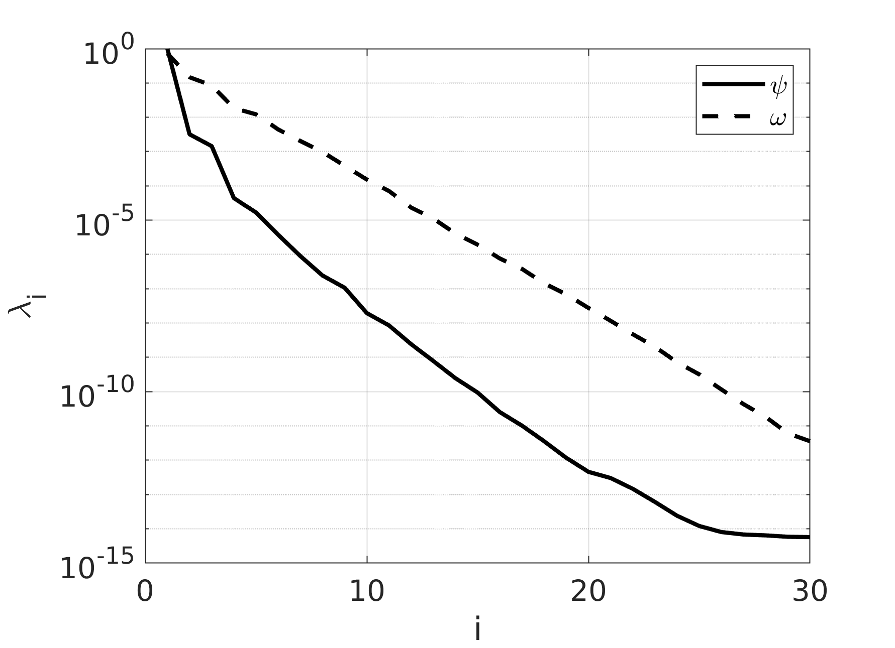
Figure 6. ROM validation - time reconstruction: eigenvalue decay for the stream function and the vorticity.

We calculate the relative $L^{2}$ error in percentage:

(35) $$E_{\Phi}(t)=100\cdot\dfrac{||\Phi_{h}(t)-\Phi_{r}(t)||_{L^{2}(\Omega)}}{||{\Phi_{h}}(t)||_{L^{2}(\Omega)}},$$

where $\Phi_{h}$ is a field computed with the FOM ($\psi_{h}$ or $\omega_{h}$) and $\Phi_{r}$ is the corresponding field computed with the ROM ($\psi_{r}$ or $\omega_{r}$). Moreover, we evaluate the relative error in percentage for the enstrophy $e=\int_{\Omega}\omega^{2}d\Omega$, i.e.:

(36) $$E_{e}(t)=100\cdot\dfrac{e_{h}(t)-e_{r}(t)}{e_{h}(t)},$$

where $e_{h}$ and $e_{r}$ are the values of the enstrophy computed by the FOM and the ROM, respectively.

Fig. 7 shows error (35) for the stream function and vorticity and error (36) for the enstrophy over time. We see that all relative errors in percentage achieve very low values. In particular, over the entire time interval the error for $\psi$ is lower than 0.4%, the error for $\omega$ is lower than 1.6%, and the error for the enstrophy is lower than 0.1% in absolute value. One observation is in order: the relative errors are significantly lower than the values obtained by ROM for the Navier–Stokes equations in primitive variables (up to 3 % for the velocity and 15 % for the pressure in the 2D flow past a cylinder benchmark [37]) We speculate that the reason for this difference could be the fact that the development of a ROM for the Navier–Stokes equations in primitive variables requires strategies for the stabilization of the pressure (e.g. supremizer enrichment and Poisson pressure equation) that makes the ROM framework more complex and error-prone [3, 12, 15, 34, 37].

\begin{overpic}[width=195.12767pt]{img/error_psi_t.png} \end{overpic}

\begin{overpic}[width=195.12767pt]{img/error_omega_t.png} \end{overpic}

\begin{overpic}[width=195.12767pt]{img/error_enstr_t.png} \end{overpic}

Figure 7. ROM validation - time reconstruction: evolution of error (35) for stream function $\psi$ (top left) and vorticity $\omega$ (top right), and error for enstrophy $e$ (36) (bottom).

In order to justify our choice to use different reduced coefficients to approximate stream-function and vorticity in (19), we show in Fig. 8 the time evolution of the first three reduced coefficients for $\psi$ and $\omega$: the differences are significant. Thus, using the same reduced coefficients would lead to a less accurate reconstruction of $\psi$ and $\omega$.

Finally, we compare the solutions computed by FOM and ROM. Fig. 9 and 10 display such comparison for $\psi$ and $\omega$ at four different times, respectively. From these figures, we see that our ROM approach provides a good global reconstruction of both stream function and vorticity. In fact, the maximum relative difference in absolute value does not exceed $4.7e-3$ for $\psi$ and $1.7e-2$ for $\omega$.

\begin{overpic}[width=195.12767pt]{img/1coeff_t.png} \end{overpic}

\begin{overpic}[width=195.12767pt]{img/2coeff_t.png} \end{overpic}

\begin{overpic}[width=195.12767pt]{img/3coeff_t.png} \end{overpic}

Figure 8. ROM validation - time reconstruction: evolution of the first three reduced coefficients for $\psi$ and $\omega$.

\begin{overpic}[width=82.38885pt]{img/psi_psiomega_4.png} \put(38.0,101.0){$t=4$} \put(-38.0,45.0){FOM} \end{overpic}

\begin{overpic}[width=82.38885pt]{img/psi_psiomega_8.png} \put(38.0,101.0){$t=8$} \end{overpic}

\begin{overpic}[width=82.38885pt]{img/psi_psiomega_16.png} \put(35.0,101.0){$t=16$} \end{overpic}

\begin{overpic}[width=82.38885pt]{img/psi_psiomega_20.png} \put(35.0,101.0){$t=20$} \end{overpic}

\begin{overpic}[width=34.69038pt]{img/legendPsiFOM.png} \end{overpic}

\begin{overpic}[width=82.38885pt]{img/psiROM_t_4.png} \put(-38.0,45.0){ROM} \end{overpic}

\begin{overpic}[width=82.38885pt]{img/psiROM_t_8.png} \end{overpic}

\begin{overpic}[width=82.38885pt]{img/psiROM_t_16.png} \end{overpic}

\begin{overpic}[width=82.38885pt]{img/psiROM_t_20.png} \end{overpic}

\begin{overpic}[width=34.69038pt]{img/legendPsiFOM.png} \end{overpic}

\begin{overpic}[width=82.38885pt]{img/psiROM_err_t_4.png} \put(-35.0,45.0){Diff.} \end{overpic}

\begin{overpic}[width=82.38885pt]{img/psiROM_err_t_8.png} \end{overpic}

\begin{overpic}[width=82.38885pt]{img/psiROM_err_t_16.png} \end{overpic}

\begin{overpic}[width=82.38885pt]{img/psiROM_err_t_20.png} \end{overpic}

\begin{overpic}[width=34.69038pt]{img/legendPsierrROM_t.png} \end{overpic}

Figure 9. ROM validation - time reconstruction: stream function $\psi$ computed by the FOM (first row) and the ROM (second row), and difference between the two fields in absolute value (third row) at times $t=4$ (first column), $t=8$ (second column), $t=16$ (third column) and $t=20$ (fourth column). We consider 6 modes.

\begin{overpic}[width=82.38885pt]{img/omega_psiomega_4.png} \put(38.0,101.0){$t=4$} \put(-38.0,45.0){FOM} \end{overpic}

\begin{overpic}[width=82.38885pt]{img/omega_psiomega_8.png} \put(38.0,101.0){$t=8$} \end{overpic}

\begin{overpic}[width=82.38885pt]{img/omega_psiomega_16.png} \put(35.0,101.0){$t=16$} \end{overpic}

\begin{overpic}[width=82.38885pt]{img/omega_psiomega_20.png} \put(35.0,101.0){$t=20$} \end{overpic}

\begin{overpic}[width=34.69038pt]{img/legendOmegaFOM.png} \end{overpic}

\begin{overpic}[width=82.38885pt]{img/omegaROM_t_4.png} \put(-38.0,45.0){ROM} \end{overpic}

\begin{overpic}[width=82.38885pt]{img/omegaROM_t_8.png} \end{overpic}

\begin{overpic}[width=82.38885pt]{img/omegaROM_t_16.png} \end{overpic}

\begin{overpic}[width=82.38885pt]{img/omegaROM_t_20.png} \end{overpic}

\begin{overpic}[width=34.69038pt]{img/legendOmegaFOM.png} \end{overpic}

\begin{overpic}[width=82.38885pt]{img/zetaROM_err_t_4.png} \put(-35.0,45.0){Diff.} \end{overpic}

\begin{overpic}[width=82.38885pt]{img/zetaROM_err_t_8.png} \end{overpic}

\begin{overpic}[width=82.38885pt]{img/zetaROM_err_t_16.png} \end{overpic}

\begin{overpic}[width=82.38885pt]{img/zetaROM_err_t_20.png} \end{overpic}

\begin{overpic}[width=34.69038pt]{img/legendZetaerrROM_t.png} \end{overpic}

Figure 10. ROM validation - time reconstruction: vorticity $\omega$ computed by the FOM (first row) and the ROM (second row), and difference between the two fields in absolute value (third row) at times $t=4$ (first column), $t=8$ (second column), $t=16$ (third column) and $t=20$ (fourth column). We consider 14 modes.

We conclude this subsection by proving some information about the efficiency of our ROM approach. The total CPU time required by a FOM simulation is about 64 s, while the computation of the modal coefficients over the entire time window of interest takes 0.47s. The resulting speed-up is about 136.

4.3. Validation of the ROM: physical parametrization

In this section, we are going to consider a physical parametric setting. We set an arbitrary array of decaying Taylor–Green vortices as source term in the vorticity equation (4) given by

(37) $$F=-\gamma e^{-t/Re}\cos(3x)\cos(3y),$$

where $\gamma$ is the strength of the source term. We consider $Re$ and $\gamma$ as the control parameters. We remark that a $Re$ parameterization has been considered in [2] and parameterization with respect to both $Re$ and $\gamma$ has been studied in [28, 29, 30] where the aim was to develop a ROM framework to account for hidden physics through data-driven strategies based on machine learning techniques. In order to reduce the offline cost, we will focus on the first half of the time interval of interest considered in Sec. 4.2, i.e. $(0,10]$.

Let us start with the parametrization with respect to $Re$ and set $\gamma=0.09$. To train the ROM, we choose a uniform sample distribution in the range $Re\in[200,800]$ with 4 sampling points: 200, 400, 600, and 800. For each value of the Reynolds number in the training set, a simulation is run over time interval $(0,10]$. Fig. 11 displays the stream function and vorticity fields computed by the FOM throughout the training set under consideration at $t=10$. We observe that the stream function does not significantly vary as $Re$ changes, while the differences in the vorticity are more evident.

Based on the results presented for the time reconstruction (Sec. 4.2), the snapshots are collected every 0.08 s. So, we collect a total of $4\times 125=500$ snapshots. We set the threshold for the selection of the eigenvalues to $1e-5$, resulting in 6 modes for $\psi$ and 11 modes for $\omega$. We take three different test values to evaluate the performance of the parametrized ROM: one value ($Re=500$) in the range under consideration but not in the training set and two values ($Re=100,1000$) outside the range under consideration. The latter cases are more challenging. Fig. 12 shows error (35) for the stream function and vorticity over time for the three values of $Re$. We see that for the interpolatory test value $Re=500$ both the errors are below 1% over the entire time interval. As for the extrapolatory test values, the errors for $Re=1000$ are comparable to the errors for $Re=500$, while the errors for $Re=100$ are much larger for $Re=100$ (up to about 3% for $\psi$ and up to about 7% for $\omega$). The poorer performance of our ROM at $Re=100$ could be due to the fact that the vorticity computed for $Re=200$ looks pretty different from the vorticity at the higher $Re$ included in the offline database (see Fig. 11). Thus, we suspect that more solutions for lower values of $Re$ would have to be included into the training set in order to obtain a more accurate reconstruction of the flow field at $Re=100$.

Fig. 13 and 14 present a qualitative comparison of the solutions computed by FOM and ROM at $t=10$ for the the three test value of $Re$. We observe that our ROM approach provides a good global reconstruction of both stream function and vorticity. In fact, the maximum relative difference in absolute value does not exceed $3.1e-2$ for $\psi$ and $6.7e-2$ for $\omega$.

Next, we consider $\gamma$ as a variable parameter and fix $Re$ to 800. Similarly to the $Re$ parameterization, the training of the ROM is carried out by a uniform sample distribution in the range $\gamma\in[0.06,0.09]$ consisting of 4 sampling points: 0.06, 0.07, 0.08 and 0.09. For each value of $\gamma$ inside the training set, a simulation is run over time interval $(0,10]$. Fig. 15 shows the stream function and vorticity fields computed by the FOM at $t=10$ for the four sampling values of $\gamma$. We see that both stream function and vorticity do not significantly vary as $\gamma$ changes value.

Analogously to what we have done for the previous parametric test case, the snapshots are collected every 0.08 s for a total of $4\times 125=500$ snapshots. We set the threshold for the selection of the eigenvalues to $1e-5$, which results in 6 modes for $\psi$ and 12 modes for $\omega$. Once again, we take three different test values to evaluate the performance of the parametrized ROM: $\gamma=0.075$ (in the range under consideration but not in the training set) and $\gamma=0.05,0.1$ (outside the range under consideration). Fig. 16 shows error (35) for the stream function and vorticity over time for these three values of $\gamma$. For the interpolatory test value ($\gamma=0.075$), the error for $\psi$ is lower than 0.4% and the error for $\omega$ is lower than 1% over the entire time interval of interest. As for the extrapolatory test values ($\gamma=0.05,0.1$), the error for $\psi$ is lower than 1.2% and the error for $\omega$ is lower than 2.5%. So, unlike the $Re$ parametric case, the errors obtained for all test values are comparable. This is obviously due to the fact that there is no abrupt change in the solution as $\gamma$ varies in $[0.06,0.09]$ (see Fig. 15) and the POD space seems to include enough information for a very good reconstruction of the flow field also at values of $\gamma$ right outside the training set.

To conclude, we qualitatively compare the solutions computed by FOM and ROM for the three test values of $\gamma$ at $t=10$ in Fig. 17 and 18. Once again, we see that our ROM approach provides a good global reconstruction of both stream function and vorticity. In fact, the maximum relative difference in absolute value does not exceed $6.3e-3$ for $\psi$ and $6.1e-2$ for $\omega$.

\begin{overpic}[width=86.72267pt,grid=false]{img/psiRe_200.png} \put(-10.0,50.0){$\psi$} \put(30.0,100.0){$Re=200$} \end{overpic}

\begin{overpic}[width=86.72267pt]{img/psiRe_400.png} \put(30.0,100.0){$Re=400$} \end{overpic}

\begin{overpic}[width=86.72267pt]{img/psiRe_600.png} \put(30.0,100.0){$Re=600$} \end{overpic}

\begin{overpic}[width=86.72267pt]{img/psiRe_800.png} \put(30.0,100.0){$Re=800$} \end{overpic}

\begin{overpic}[width=31.65341pt]{img/scale_psi_Re.png} \end{overpic}

\begin{overpic}[width=95.39693pt]{img/zetaRe_200.png} \put(-5.0,50.0){$\omega$} \end{overpic}

\begin{overpic}[width=95.39693pt]{img/zetaRe_400.png} \end{overpic}

\begin{overpic}[width=95.39693pt]{img/zetaRe_600.png} \end{overpic}

\begin{overpic}[width=95.39693pt]{img/zetaRe_800_1.png} \end{overpic}

\begin{overpic}[width=31.65341pt]{img/scale_zeta_Re.png} \end{overpic}

Figure 11. ROM validation - $Re$ parameterization: stream function $\psi$ (first row) and vorticity $\omega$ (second row) computed by the FOM at $Re=200$ (first column), $Re=400$ (second column), $Re=600$ (third column), and $Re=800$ (fourth column), at time $t=10$ for $\gamma=0.09$.

\begin{overpic}[width=195.12767pt]{img/err_Re_psi.png} \end{overpic}

\begin{overpic}[width=195.12767pt]{img/err_Re_omega.png} \end{overpic}

Figure 12. ROM validation - $Re$ parameterization: time history of error (35) for stream function $\psi$ (left) and vorticity $\omega$ (right) for three different test values: $Re=100$, $Re=500$ and $Re=1000$.

\begin{overpic}[width=75.88481pt]{img/psiFOM_100_0_09.png} \put(20.0,103.0){$Re=100$} \put(-42.0,45.0){FOM} \end{overpic}

\begin{overpic}[width=32.52017pt]{img/legenda_100_0_09_psi.png} \end{overpic}

\begin{overpic}[width=75.88481pt]{img/psiFOM_500_0_09.png} \put(20.0,103.0){$Re=500$} \end{overpic}

\begin{overpic}[width=32.52017pt]{img/legenda_500_0_09_psi.png} \end{overpic}

\begin{overpic}[width=75.88481pt]{img/psiFOM_500_0_09.png} \put(20.0,103.0){$Re=1000$} \end{overpic}

\begin{overpic}[width=32.52017pt]{img/legenda_1000_0_09_psi.png} \end{overpic}

\begin{overpic}[width=75.88481pt]{img/psiROM_100_0_09.png} \put(-42.0,45.0){ROM} \end{overpic}

\begin{overpic}[width=32.52017pt]{img/legenda_100_0_09_psi.png} \end{overpic}

\begin{overpic}[width=75.88481pt]{img/psiROM_500_0_09.png} \end{overpic}

\begin{overpic}[width=32.52017pt]{img/legenda_500_0_09_psi.png} \end{overpic}

\begin{overpic}[width=75.88481pt]{img/psiROM_1000_0_09.png} \end{overpic}

\begin{overpic}[width=32.52017pt]{img/legenda_1000_0_09_psi.png} \end{overpic}

\begin{overpic}[width=78.04842pt]{img/errpsi_100_0_09.png} \put(-32.0,45.0){Diff.} \end{overpic}

\begin{overpic}[width=33.38693pt]{img/legenda_100_0_09_err_psi.png} \end{overpic}

\begin{overpic}[width=78.04842pt]{img/errpsi_500_0_09.png} \end{overpic}

\begin{overpic}[width=32.52017pt]{img/legenda_500_0_09_err_psi.png} \end{overpic}

\begin{overpic}[width=78.04842pt]{img/errpsi_1000_0_09.png} \end{overpic}

\begin{overpic}[width=32.52017pt]{img/legenda_1000_0_09_err_psi.png} \end{overpic}

Figure 13. ROM validation - $Re$ parameterization: stream function $\psi$ computed by the FOM (first row) and the ROM (second row), and difference between the two fields in absolute value (third row) for $Re=100$ (first column), $Re=500$ (second column) and $Re=1000$ (third one) at time $t=10$. Six modes for $\psi$ were considered.

\begin{overpic}[width=75.88481pt]{img/zetaFOM_100_0_09.png} \put(25.0,103.0){$Re=100$} \put(-42.0,45.0){FOM} \end{overpic}

\begin{overpic}[width=28.18636pt]{img/legenda_100_0_09_zeta.png} \end{overpic}

\begin{overpic}[width=75.88481pt]{img/zetaFOM_500_0_09.png} \put(25.0,103.0){$Re=500$} \end{overpic}

\begin{overpic}[width=28.18636pt]{img/legenda_500_0_09_zeta.png} \end{overpic}

\begin{overpic}[width=75.88481pt]{img/zetaFOM_1000_0_09.png} \put(25.0,103.0){$Re=1000$} \end{overpic}

\begin{overpic}[width=28.18636pt]{img/legenda_1000_0_09_zeta.png} \end{overpic}

\begin{overpic}[width=75.88481pt]{img/zetaROM_100_0_09.png} \put(-42.0,45.0){ROM} \end{overpic}

\begin{overpic}[width=28.18636pt]{img/legenda_100_0_09_zeta.png} \end{overpic}

\begin{overpic}[width=75.88481pt]{img/zetaROM_500_0_09.png} \end{overpic}

\begin{overpic}[width=28.18636pt]{img/legenda_500_0_09_zeta.png} \end{overpic}

\begin{overpic}[width=75.88481pt]{img/zetaROM_1000_0_09.png} \end{overpic}

\begin{overpic}[width=28.18636pt]{img/legenda_1000_0_09_zeta.png} \end{overpic}

\begin{overpic}[width=80.21863pt]{img/errzeta_100_0_09.png} \put(-32.0,45.0){Diff.} \end{overpic}

\begin{overpic}[width=33.38693pt]{img/legenda_100_0_09_err_zeta.png} \end{overpic}

\begin{overpic}[width=80.21863pt]{img/errzeta_500_0_09.png} \end{overpic}

\begin{overpic}[width=32.52017pt]{img/legenda_500_0_09_err_zeta.png} \end{overpic}

\begin{overpic}[width=80.21863pt]{img/errzeta_1000_0_09.png} \end{overpic}

\begin{overpic}[width=32.52017pt]{img/legenda_1000_0_09_err_zeta.png} \end{overpic}

Figure 14. ROM validation - $Re$ parameterization: vorticity $\omega$ computed by the FOM (first row) and the ROM (second row), and difference between the two fields in absolute value (third row) for $Re=100$ (first column), $Re=500$ (second column) and $Re=1000$ (third one) at time $t=10$. Eleven modes for $\omega$ were considered.

\begin{overpic}[width=91.0631pt]{img/psiRe_800_0_06.png} \put(-10.0,50.0){$\psi$} \put(30.0,100.0){$\gamma=0.06$} \end{overpic}

\begin{overpic}[width=91.0631pt]{img/psiRe_800_0_07.png} \put(30.0,100.0){$\gamma=0.07$} \end{overpic}

\begin{overpic}[width=91.0631pt]{img/psiRe_800_0_08.png} \put(30.0,100.0){$\gamma=0.08$} \end{overpic}

\begin{overpic}[width=91.0631pt]{img/psiRe_800.png} \put(30.0,100.0){$\gamma=0.09$} \end{overpic}

\begin{overpic}[width=31.65341pt]{img/scale_psi_Re.png} \end{overpic}

\begin{overpic}[width=91.0631pt]{img/zetaRe_800_0_06.png} \put(-10.0,50.0){$\omega$} \end{overpic}

\begin{overpic}[width=91.0631pt]{img/zetaRe_800_0_07.png} \end{overpic}

\begin{overpic}[width=91.0631pt]{img/zetaRe_800_0_08.png} \end{overpic}

\begin{overpic}[width=91.0631pt]{img/zetaRe_800.png} \end{overpic}

\begin{overpic}[width=31.65341pt]{img/scale_zeta_Re.png} \end{overpic}

Figure 15. ROM validation - $\gamma$ parameterization: stream function $\psi$ (first row) and vorticity $\omega$ (second row) computed by the FOM for $Re=800$ and $\gamma=0.06$ (first column), $\gamma=0.07$ (second column), $\gamma=0.08$ (third column), and $\gamma=0.09$ (fourth column) at time $t=10$.

\begin{overpic}[width=195.12767pt]{img/err_gamma_psi.png} \end{overpic}

\begin{overpic}[width=195.12767pt]{img/err_gamma_omega.png} \end{overpic}

Figure 16. ROM validation - $\gamma$ parameterization: time history of error (35) for stream function $\psi$ (left) and vorticity $\omega$ (right) for the three different test values $\gamma=0.05$, $\gamma=0.075$ and $\gamma=0.1$ at $Re=800$.

\begin{overpic}[width=75.88481pt]{img/psiFOM_800_0_05.png} \put(22.0,103.0){$\gamma=0.05$} \put(-42.0,48.0){FOM} \end{overpic}

\begin{overpic}[width=32.52017pt]{img/legenda_800_0_05_psi.png} \end{overpic}

\begin{overpic}[width=75.88481pt]{img/psiFOM_800_0_075.png} \put(20.0,103.0){$\gamma=0.075$} \end{overpic}

\begin{overpic}[width=32.52017pt]{img/legenda_800_0_05_psi.png} \end{overpic}

\begin{overpic}[width=75.88481pt]{img/psiFOM_800_0_1.png} \put(24.0,103.0){$\gamma=0.1$} \end{overpic}

\begin{overpic}[width=32.52017pt]{img/legenda_800_0_05_psi.png} \end{overpic}

\begin{overpic}[width=75.88481pt]{img/psiROM_800_0_05.png} \put(-42.0,48.0){ROM} \end{overpic}

\begin{overpic}[width=32.52017pt]{img/legenda_800_0_05_psi.png} \end{overpic}

\begin{overpic}[width=75.88481pt]{img/psiROM_800_0_075.png} \end{overpic}

\begin{overpic}[width=32.52017pt]{img/legenda_800_0_05_psi.png} \end{overpic}

\begin{overpic}[width=75.88481pt]{img/psiROM_800_0_1.png} \end{overpic}

\begin{overpic}[width=32.52017pt]{img/legenda_800_0_05_psi.png} \end{overpic}

\begin{overpic}[width=80.21863pt]{img/errpsi_800_0_05.png} \put(-32.0,48.0){Diff.} \end{overpic}

\begin{overpic}[width=28.18636pt]{img/legenda_800_0_05_err_psi.png} \end{overpic}

\begin{overpic}[width=75.88481pt]{img/errpsi_800_0_075.png} \end{overpic}

\begin{overpic}[width=28.18636pt]{img/legenda_800_0_075_err_psi.png} \end{overpic}

\begin{overpic}[width=75.88481pt]{img/errpsi_800_0_1.png} \end{overpic}

\begin{overpic}[width=28.18636pt]{img/legenda_800_0_1_err_psi.png} \end{overpic}

Figure 17. ROM validation - $\gamma$ parameterization: stream function $\psi$ computed by the FOM (first row) and the ROM (second row), and difference between the two fields in absolute value (third row) for $\gamma=0.05$ (first column), $\gamma=0.075$ (second column) and $\gamma=0.1$ (third one) at time $t=10$. Six modes for $\psi$ were considered.

\begin{overpic}[width=75.88481pt]{img/zetaFOM_800_0_05.png} \put(22.0,103.0){$\gamma=0.05$} \put(-42.0,48.0){FOM} \end{overpic}

\begin{overpic}[width=28.18636pt]{img/legenda_800_0_05_zeta.png} \end{overpic}

\begin{overpic}[width=75.88481pt]{img/zetaFOM_800_0_075.png} \put(20.0,103.0){$\gamma=0.075$} \end{overpic}

\begin{overpic}[width=30.35657pt]{img/legenda_800_0_075_zeta.png} \end{overpic}

\begin{overpic}[width=75.88481pt]{img/zetaFOM_800_0_1.png} \put(20.0,103.0){$\gamma=0.1$} \end{overpic}

\begin{overpic}[width=28.18636pt]{img/legenda_800_0_1_zeta.png} \end{overpic}

\begin{overpic}[width=75.88481pt]{img/zetaROM_800_0_05.png} \put(-42.0,48.0){ROM} \end{overpic}

\begin{overpic}[width=28.18636pt]{img/legenda_800_0_05_zeta.png} \end{overpic}

\begin{overpic}[width=75.88481pt]{img/zetaROM_800_0_075.png} \end{overpic}

\begin{overpic}[width=30.35657pt]{img/legenda_800_0_075_zeta.png} \end{overpic}

\begin{overpic}[width=75.88481pt]{img/zetaROM_800_0_1.png} \end{overpic}

\begin{overpic}[width=30.35657pt]{img/legenda_800_0_1_zeta.png} \end{overpic}

\begin{overpic}[width=75.88481pt]{img/errzeta_800_0_05.png} \put(-32.0,48.0){Diff.} \end{overpic}

\begin{overpic}[width=30.35657pt]{img/legenda_800_0_05_err_zeta.png} \end{overpic}

\begin{overpic}[width=75.88481pt]{img/errzeta_800_0_075.png} \end{overpic}

\begin{overpic}[width=30.35657pt]{img/legenda_800_0_075_err_zeta.png} \end{overpic}

\begin{overpic}[width=75.88481pt]{img/errzeta_800_0_1.png} \end{overpic}

\begin{overpic}[width=30.35657pt]{img/legenda_800_0_1_err_zeta.png} \end{overpic}

Figure 18. ROM validation - $\gamma$ parameterization: vorticity $\omega$ computed by the FOM (first row) and the ROM (second row), and difference between the two fields in absolute value (third row) for $\gamma=0.05$ (first column), $\gamma=0.075$ (second column) and $\gamma=0.1$ (third one) at time $t=10$. Twelve modes for $\omega$ were considered.

5. Conclusions and future developments

This work presents a POD-Galerkin based Reduced Order Method for the Navier–Stokes equations in stream function-vorticity formulation within a Finite Volume environment. The main novelties of the proposed ROM approach are: (i) the use of different coefficients to approximate the stream function and vorticity fields and (ii) the use of a global POD basis space for parametric studies. We assessed our ROM approach with the vortex merger problem, a classical benchmark used for the validation of numerical methods for the stream function-vorticity formulation of the Navier–Stokes equations. The numerical results show that our ROM is able to capture the flow features with a good accuracy both in the reconstruction of the flow field evolution and in a physical parametric setting. In addition, for the simple vortex merger problem we observed that our ROM enables substantial computational time savings.

Next, we are going to extend the ROM approach presented here to the Quasi-Geostrophic Equations. In particular, we intend to couple such equations with a differential filter [11, 12, 13, 15, 14] in order to simulate two-dimensional turbulent geophysical flows on under-refined meshes in the spirit of [16, 24].

References

- [1] S. Ahmed, S. M. Rahman, O. San, A. Rasheed, and I. Navon. Memory embedded non-intrusive reduced order modeling of non-ergodic flows. Physics of Fluids, 31:126602, 2019.
- [2] S. Ahmed, O. San, A. Rasheed, and T. Iliescu. A long short-term memory embedding for hybrid uplifted reduced order models. Physica D: Nonlinear Phenomena, 409:132471, 2020.
- [3] F. Ballarin, A. Manzoni, A. Quarteroni, and G. Rozza. Supremizer stabilization of POD–Galerkin approximation of parametrized steady incompressible Navier–Stokes equations. International Journal for Numerical Methods in Engineering, 102:1136–1161, 2014.
- [4] M. Behr, R. Liou, J.and Shih, and T. Tezduyar. Vorticity‐streamfunction formulation of unsteady incompressible flow past a cylinder: Sensitivity of the computed flow field to the location of the outflow boundary. International Journal for Numerical Methods in Fluids, 12:323–342, 1991.
- [5] P. Benner, W. Schilders, S. Grivet-Talocia, A. Quarteroni, G. Rozza, and L. M. Silveira. Model Order Reduction. De Gruyter, Berlin, Boston, 2020.
- [6] J. Burkardt, M. Gunzburger, and H.-C. Lee. POD and CVT-based reduced-order modeling of Navier–Stokes flows. Computer Methods in Applied Mechanics and Engineering, 196:337–355, 2006.
- [7] F. Chinesta, A. Huerta, G. Rozza, and K. Willcox. Model Order Reduction. Encyclopedia of Computational Mechanics, Elsevier Editor, 2016.
- [8] F. Chinesta, P. Ladeveze, and E. Cueto. A Short Review on Model Order Reduction Based on Proper Generalized Decomposition. Archives of Computational Methods in Engineering, 18:395, 2011.
- [9] A. Dumon, C. Allery, and A. Ammar. Proper generalized decomposition method for incompressible flows in stream-vorticity formulation. European Journal of Computational Mechanics, 19:591–617, 2010.
- [10] A. Dumon, C. Allery, and A. Ammar. Proper General Decomposition (PGD) for the resolution of Navier-Stokes equations. Journal of Computational Physics, 230:1387–1407, 2011.
- [11] M. Girfoglio, A. Quaini, and G.Rozza. Fluid–structure interaction simulations with a LES filtering approach in solids4Foam. Communications in Applied and Industrial Mathematics, 12:13–28, 2021.
- [12] M. Girfoglio, A. Quaini, and G.Rozza. Pressure stabilization strategies for a LES filtering Reduced Order Model. Fluids, 6:302, 2021.
- [13] M. Girfoglio, A. Quaini, and G. Rozza. A Finite Volume approximation of the Navier-Stokes equations with nonlinear filtering stabilization. Computers & Fluids, 187:27–45, 2019.
- [14] M. Girfoglio, A. Quaini, and G. Rozza. A Hybrid Reduced Order Model for nonlinear LES filtering. https://arxiv.org/abs/2107.12933, 2021.
- [15] M. Girfoglio, A. Quaini, and G. Rozza. A POD-Galerkin reduced order model for a LES filtering approach. Journal of Computational Physics, 436:110260, 2021.
- [16] D. Holm and B. Nadiga. Modeling mesoscale turbulence in the barotropic double-gyre circulation. Journal of Physical Oceanography, 33:2355–2365, 2003.
- [17] R. I. Issa. Solution of the implicitly discretised fluid flow equations by operator-splitting. Journal of Computational Physics, 62:40–65, 1986.
- [18] H. Jasak. Error analysis and estimation for the finite volume method with applications to fluid flows. PhD thesis, Imperial College, University of London, 1996.
- [19] I. Kalashnikova and M. F. Barone. On the stability and convergence of a Galerkin reduced order model (ROM) of compressible flow with solid wall and far-field boundary treatment. International Journal for Numerical Methods in Engineering, 83:1345–1375, 2010.
- [20] K. Kunisch and S. Volkwein. Galerkin proper orthogonal decomposition methods for a general equation in fluid dynamics. SIAM Journal on Numerical Analysis, 40:492–515, 2002.
- [21] J. Lequeurre and A. Munnier. orticity and Stream Function Formulations for the 2D Navier–Stokes Equations in a Bounded Domain. Journal of Mathematical Fluid Mechanics, 22, 2020.
- [22] S. Lorenzi, A. Cammi, L. Luzzi, and G. Rozza. POD-Galerkin method for finite volume approximation of Navier–Stokes and RANS equations. Computer Methods in Applied Mechanics and Engineering, 311:151–179, 2016.
- [23] P. Minev and P. Vabishchevich. An operator-splitting scheme for the stream function–vorticity formulation of the unsteady Navier–Stokes equations. Journal of Computational and Applied Mathematics, 293:147–163, 2015.
- [24] I. Monteiro, C. Manica, and L. Rebholz. Numerical study of a regularized barotropic vorticity model of geophysical flow. Numerical Methods for Partial Differential Equations, 31:1492–1514, 2015.
- [25] Z. Mou, C.and Wang, D. Wells, X. Xie, and T. Iliescu. Reduced order models for the quasi-geostrophic equations: A brief survey. Fluids, 6:16, 2020.
- [26] F. Moukalled, L. Mangani, and M. Darwish. The Finite Volume Method in Computational Fluid Dynamics: An Advanced Introduction with OpenFOAM and Matlab. 1st ed., Springer Publishing Company, Incorporated, 2015.
- [27] S. V. Patankar and D. B. Spalding. A calculation procedure for heat, mass and momentum transfer in three-dimensional parabolic flows. International Journal of Heat and Mass Transfer, 15:1787–1806, 1972.
- [28] S. Pawar, S. Ahmed, O. San, and A. Rasheed. Data-driven recovery of hidden physics in reduced order modeling of fluid flows. Physics of Fluids, 32:036602, 2020.
- [29] S. Pawar, S. Ahmed, O. San, and A. Rasheed. An evolve-then-correct reduced order model for hidden fluid dynamics. Mathematics, 8:570, 2020.
- [30] S. Pawar, O. San, A. Nair, A. Rasheed, and T. Kvamsdal. Model fusion with physics-guided machine learning: Projection-based reduced-order modeling. Physics of Fluids, 33:067123, 2021.
- [31] A. Quarteroni, A. Manzoni, and F. Negri. Reduced Basis Methods for Partial Differential Equations. Springer International Publishing, 2016.
- [32] J. Reinaud and D. Dritschel. The critical merger distance between two co-rotating quasi-geostrophic vortices. Journal of Fluid Mechanics, 522:357–381, 2005.
- [33] G. Rozza, D. B. P. Huynh, and A. T. Patera. Reduced Basis Approximation and a Posteriori Error Estimation for Affinely Parametrized Elliptic Coercive Partial Differential Equations. Archives of Computational Methods in Engineering, 15:229, 2008.
- [34] G. Rozza and K. Veroy. On the stability of the reduced basis method for Stokes equations in parametrized domains. Computer Methods in Applied Mechanics and Engineering, 196:1244–1260, 2007.
- [35] O. San and J. Borggaard. Principal interval decomposition framework for POD reduced-order modeling of convective Boussinesq flows. International Journal for Numerical Methods in Fluids, 78:37–62, 2015.
- [36] E. Sousa and I. Sobey. Effect of boundary vorticity discretization on explicit stream‐function vorticity calculations. International Journal for Numerical Methods in Fluids, 49:371–393, 2005.
- [37] G. Stabile and G. Rozza. Finite volume POD-Galerkin stabilised reduced order methods for the parametrised incompressible Navier–Stokes equations. Computer & Fluids, 173:273–284, 2018.
- [38] S. Kelbij Star, Giovanni Stabile, Francesco Belloni, Gianluigi Rozza, and Joris Degroote. A novel iterative penalty method to enforce boundary conditions in finite volume pod-galerkin reduced order models for fluid dynamics problems. Communications in Computational Physics, 30:34–66, 2021.
- [39] R. Temam. Navier-Stokes Equations: Theory and Numerical Analysis. Cambridge University Press, 2001.
- [40] T. Tezduyar, J. Liou, and D.K. Ganjoo. Incompressible flow computations based on the vorticity-stream function and velocity-pressure formulations. Computers & Structures, 35:445–472, 1990.
- [41] K. Veroy and A. T. Patera. Certified real-time solution of the parametrized steady incompressible navier-stokes equations: Rigorous reduced-basis a posteriori error bounds. International Journal for Numerical Methods in Fluids, 47:773–788, 2005.
- [42] H. G. Weller, G. Tabor, H. Jasak, and C. Fureby. A tensorial approach to computational continuum mechanics using object-oriented techniques. Computers in physics, 12(6):620–631, 1998.