Coherence of probabilistic constraints on Nash equilibria

Abstract

Observable games are game situations that reach one of possibly many Nash equilibria. Before an instance of the game starts, an external observer does not know, a priori, what is the exact profile of actions that will occur; thus, he assigns subjective probabilities to players’ actions. However, not all probabilistic assignments are coherent with a given game. We study the decision problem of determining if a given set of probabilistic constraints assigned a priori by the observer to a given game is coherent, which we call the Coherence of Probabilistic Constraints on Equilibria, or PCE-Coherence. We show several results concerning algorithms and complexity for PCE-Coherence when only pure Nash equilibria are considered. In this context, we also study the computation of maximal and minimal probabilistic constraints on actions that preserves coherence. Finally, we study these problems when mixed Nash equilibria are allowed.

Keywords. Nash equilibrium, uncertain game, probabilistic constraints, coherence of constraints, computational complexity

1 Introduction

In game theory, a Nash equilibrium represents a situation in which each player’s strategy is a best response to other players’ strategies; thus no player can obtain gains by changing alone his/her own strategy. Nash proved that every $n$-player, finite, non-cooperative game has a mixed-strategy equilibrium point [NashNash1950b, NashNash1950a, NashNash1951]; however, more than one equilibrium may exist and the number of equilibria can be even exponentially large over some game parameters.

For an observer knowing that an equilibrium is to be reached, there is an a priori uncertainty before an instance of the game starts, concerning the exact kind of equilibrium to be reached and also in knowing the players’ actions in that instance. Due to the computational complexity in explicitly producing the set of equilibrium states, the observer considers that set as hidden or latent. Therefore, it is most natural to describe the observer’s uncertainty in terms of subjective probabilities assigned to actions in those equilibrium states, in which one presupposes a probability distribution over the set of all possible equilibria. Our aim in this work is to study such a scenario comprehending a game and an observer, which we call an observable game.

We assume that the players involved in a game always react to each other with a best response in such a way that, since the game starts, its dynamics converge to an equilibrium. The intermediate steps where an equilibrium has not been achieved yet are not covered by the model, since the observer is only interested in the final stable outcome. In case there are only two players and the first one to take an action does it smartly so that he will not need to change, the only source of randomness ends up being who will be the first player to take an action unless such action puts the second player in a position to choose among tied best responses. In any case, the proposed model aggregates all the possibilities of randomness concerning the actions to be taken.

A way for the external observer to assign subjective probabilities to actions is looking at the past reactions of the players involved in a game situation that repeatedly happens. The configuration of the repeating games may even change from one instance to another regarding the allowed actions to each player or the utility values associated with the action profiles, however the observer may be able to grasp what kind of reaction is more likely to each player by observing the outcomes of the previous games.

Unfortunately, not every assignment on action probabilities by an observer finds correspondence to an actual probability distribution on possible equilibria of a given game; in fact, some actions may always co-occur at equilibrium, so constraining their probabilities to distinct values does not correspond to any underlying distribution on equilibria. In case the observer assigns a set of probabilistic constraints on actions that correspond to a probability distribution on equilibria, we say the observable game is coherent.

Lack of coherence can have important consequences which are better seen in a betting scenario where an observer knows the configuration of a game before one of its instances is played, and also knows that this game reaches an equilibrium. The observer wants to place bets on the occurrence of actions and an incoherent set of probabilities may lead to sure loss. So detecting and avoiding such a disastrous assignment of probabilities may have considerable cost to the observer. This betting scenario corresponds to de Finetti’s interpretation of subjective probabilities [de Finettide Finetti1931, de Finettide Finetti2017] in which incoherent probabilities have a one-to-one correspondence to sure loss. An actual scenario of this kind may be seen in the pricing strategy of oligopolistic markets. We introduce the following motivational example.

Motivational Example

Assume that Madeira Beverages is a local beverages company in Madeira island that sells as its main product, beers. Two companies dominate the country beer market. They price their products from time to time in light of competition aiming to conquer the largest market share and make the most profit. Among the mechanisms of sale strategies there are price promotions (short-term price reductions), thus the price portfolio of a company in some period is not of public knowledge in advance. However, it is very reasonable to assume that the profits of the companies in the oligopoly reach an equilibrium during the sales period under consideration. Oblivious to the oligopoly competition, it is of great interest to Madeira Beverages to predict the price portfolios of the big companies based on its experience in observing their competition and pricing strategies; such prediction might help it to set up its own pricing strategy and even his production process, which takes place in a small and more limited industry. This information may be crucial, for example, for deciding to limit the production of beers that cannot be competitive with the oligopoly price portfolios of that period and focus on the production of some other beers with a more targeted niche or launch new non-beer products. In this scenario, the big companies, their price portfolios, and their profits (which may be inferred from their price portfolios), are respectively the players, their actions, and their utilities in a game; the local producer with predictions about the oligopolistic market is the observer with subjective probabilities over the player’s actions.

In this work, we formalize such scenario with a market in equilibrium and an external agent who has some idea about that equilibrium but is uncertain on the probabilistic distribution on the possible equilibria and therefore on the players’ actions. Of course, there may be aspects left out as it is expected from any theoretical idealization of the real world.

We study the following problems related to observable games according to pure and mixed Nash equilibrium over some different classes of games:

The Coherence Problem

Given an observable game — a game together with a set of probabilistic constraints on its actions —, decide if it is coherent; that is, decide if there exists an actual probability distribution on the game equilibria that corresponds to those probabilistic constraints.

The Extension (Inference) Problem

Given a coherent observable game with probabilistic assignments on some of the players’ actions, compute upper and lower bounds on the probabilities of some other action that preserves coherence.

We can divide the study of equilibrium problems in two fundamental aspects. On the one hand, the model per se; in this case, equilibrium concepts are often understood as models that explain (rational or not) agent behavior, e.g. in the markets or in a biological system. On the other hand, algorithms; such issues become relevant in the cases where it is important to actually compute an equilibrium. Coherence of observable games — or, coherence of probabilistic constraints on equilibria — does not constitute a concept of equilibrium, however we can make an analogy between their study and the two aforementioned aspects. Indeed, the main goals of this work are:

• Formalize the concept of coherent observable games; we also deepen the discussion on the kind of phenomena such concept model.

• Solve the Coherence and Extension Problems.

In the conclusions we propose an attempted explanation on how the algorithmic aspects may affect the phenomena modeled by (in)coherent observable games.

The combination of uncertainty and game equilibria is not trivial, so in order to better understand it we initially concentrate on uncertainty over pure equilibria, a restricted form of mixed-strategy equilibria in which each player chooses a unique action strategy, and whose existence is not even guaranteed. That is, the observer knows a priori that a pure equilibrium is to be reached for a given game, but does not know exactly which action strategies will be performed at equilibrium.

We later consider uncertainty in mixed-strategy equilibria, a doubly uncertain situation, that combines uncertainty on the actions to be played in a specific instance of a game with the probabilistic notion of mixed-strategy. It is important to note that the notion of probability on equilibria is different from that of mixed-strategy equilibrium; in fact, these two notions are independent. The former deals with a probability distribution on possible equilibria, and the latter allows for probability distribution on an agent’s actions as part of the player’s strategy.

The paper is organized as follows. In Section 2 we define the preliminary notions of game, observable game, action profile, and pure Nash equilibrium. The concept of coherent observable game, and Coherence and Extension problems in the restricted setting of pure equilibria are formally defined in Section 3. In Section 4 we show the linear algebraic formulation of Coherence and Extension problems, we show some complexity and inapproximability results and propose solutions to the problems via reduction results; we also discuss the relations between Coherence and Probabilistic Satisfiability problems. In Section 5 we generalize all the concepts and problems to the setting which includes mixed Nash equilibria; we discuss algorithms and show complexity and inapproximability results.

2 Preliminaries

We define a game as a quadruple $G=\langle{P,N,A,u}\rangle$, where $P=\{1,\ldots,n\}$ lists the $n$ players in the game, $N=\langle{N_{1},\ldots,N_{n}}\rangle$ is a sequence of player neighborhoods, in which $N_{i}\subset P\setminus\{i\}$ is the set of player $i$ neighbors, $A=A_{1}\times\cdots\times A_{n}$ is a set of action profiles, in which each $A_{i}$ is the set of all possible actions for player $i$, and $u=\langle{u_{1},\ldots,u_{n}}\rangle$ is a sequence of utility functions in which $u_{i}:A\to\mathbb{Q}$ is the utility function for player $i$. Assume that $A_{i}\cap A_{j}=\varnothing$ for player $i\neq j$, and that $u_{i}(a_{1},\ldots,a^{\prime}_{j},\ldots,a_{n})=u_{i}(a_{1},\ldots,a^{\prime\prime}_{j},\ldots,a_{n})$ for $j\notin N_{i}\cup\{i\}$.

An action profile $e=\langle{a_{1},\ldots,a_{i},\ldots,a_{n}}\rangle$ is a pure (Nash) equilibrium if, for every player $i$, $u_{i}(e)\geq u_{i}(a_{1},\ldots,a^{\prime}_{i},\ldots,a_{n})$ for every $a^{\prime}_{i}\in A_{i}$. A game $G$ may have zero or more pure equilibria. We write $a_{i}\in e$ to express that $a_{i}$ is the $i$th component of $e$.

By an observable game we mean a pair $\mathcal{G}=\langle{G,\Pi}\rangle$ where $G$ is a game and $\Pi$ is a set of probabilistic constraints on equilibria (PCE), that is a set of probability assignments on actions limiting the probabilities of some actions occurring in an equilibrium, which represents the observer’s ignorance on what equilibrium will be reached; we assume it has the following format:

$$\Pi=\Big{\{}P(\alpha_{k})~{}\bowtie_{k}~{}p_{k}~{}\Big{|}~{}\bowtie_{k}\in\{\leq,\geq,=\},1\leq k\leq K\Big{\}},$$

where $\alpha_{k}$ are actions and $p_{k}$ are values in $[0,1]\cap\mathbb{Q}$. Formally, a set of PCE is a set of triples $\Pi=\{\langle{\alpha_{k},\bowtie_{k},p_{k}}\rangle,1\leq k\leq K\}$.

3 Formalizing the concept

As observable games deal with the scenario where an equilibrium is to be reached but its action profile is unknown, we assign probabilities to equilibria: let $E_{G}=\{e_{1},\ldots,e_{M}\}$ be the set of all equilibria associated with game $G$; we consider a probability function over $G$-equilibria $P:E_{G}\to[0,1]\cap\mathbb{Q}$, such that $P(e_{i})\geq 0$ and $\sum_{e_{i}\in E_{G}}P(e_{i})=1$. We define the probability $P(a_{i})$ that $a_{i}\in e\in E_{G}$ is executed in a game $G$ as

$$P(a_{i})=\sum_{j\,|\,a_{i}\in e_{j}}P(e_{j}).$$

Given a game $G$ and an equilibrium probability function $P$, it is possible to compute the probability of any action; however we face two problems. First, the number of equilibria may be exponentially large in the numbers of players and of actions allowed for players. Second, we may not know the equilibrium probability function $P$. Instead we are presented with an observable game $\mathcal{G}=\langle{G,\Pi}\rangle$, where $G$ is a game and $\Pi$ is a set of PCE and we are asked to decide the existence of an underlying probability function $P$ that satisfies $\Pi$; and, in case one exists, we want to compute the range of probabilities for an unconstrained action $a_{i}$. The former problem is called the probabilistic coherence problem and the second one is the probabilistic extension problem.

Definition 1 (PCE Coherence Problem)

Given an observable game $\mathcal{G}=\langle{G,\Pi}\rangle$, PCE-Coherence consists of deciding if it is coherent, that is if there exists a probability function over the set of $G$-equilibria that satisfies all constraints in $\Pi$. PCE-Coherence rejects the instance if it is not coherent or if there exists no equilibrium in $G$. _□

Definition 2 (PCE Extension Problem)

Let $\mathcal{G}$ be a coherent observable game. Given an action $a_{i}\in A_{i}$, PCE-Extension consists in finding probability functions $\underline{P}$ and $\overline{P}$ that satisfy $\Pi$ such that $\underline{P}(a_{i})$ is minimal and $\overline{P}(a_{i})$ is maximal. _□

The coherence of an observable game models the interaction that the uncertainty about the game should have with the knowledge that such game reaches equilibrium. Thus, an incoherent observable game explains the inevitable failure of the observer in taking advantage of his position of observer, e.g. the sure loss of the better in de Finetti’s probability interpretation or the poor management of the local beer producer observing the oligopolistic market. However, it is important to notice that the observer’s subjective probability assignments may be coherent and still far from reality. In this way, an incoherent observable game alone may be enough to explain the failure of the observer, but a coherent observable game is not enough to guarantee his success. All in all, the sharpness of the observer’s probability assignments also depends on how deep is his knowledge about the game and to be coherent is only part of his enterprise in making a good analysis of the game he observes.

Example 1

Suppose we have a game between Alice and Bob in which Alice has three possible actions $a^{1}$, $a^{2}$, and $a^{3}$, and Bob also has three possible actions $b^{1}$, $b^{2}$, and $b^{3}$, such that the joint utilities are given by Table 1. This game has three pure Nash equilibria: $\langle{a^{1},b^{1}}\rangle$, $\langle{a^{2},b^{3}}\rangle$, and $\langle{a^{3},b^{3}}\rangle$, which are stressed in bold.

	$b^{1}$	$b^{2}$	$b^{3}$
$a^{1}$	$\mathbf{2,2}$	$1,1$	$1,0$
$a^{2}$	$1,2$	$5,4$	$\mathbf{1,5}$
$a^{3}$	$0,1$	$2,3$	$\mathbf{1,3}$

Table 1: Utility functions for Alice and Bob.

Suppose the game will reach a pure equilibrium state, in which case Bob and Alice will have chosen to play a single action; we now want to see through an external observer’s eyes who does not know which equilibrium will be reached, however gives to the action $a^{2}$ the probability of $\frac{1}{3}$. Is this restriction feasible (coherent)? And if it is, what is the lower bound on the probability of Bob playing $b^{3}$ this observer should assign in order to remain coherent? Can it be, say, $\frac{1}{4}$?

Let us formalize such situation by $\mathcal{G}_{1}=\langle{G_{1},\Pi_{1}}\rangle$, where $G_{1}=\langle{P,N,A,u}\rangle$, in which $P=\{a,b\}$, $N_{i}=P\setminus\{i\}$, $A_{a}=\{a^{1},a^{2},a^{3}\}$, $A_{b}=\{b^{1},b^{2},b^{3}\}$, and $u$ is given by Table 1. In $\Pi_{1}$, we consider the action $a^{2}$ occurring in an equilibrium with constraint $P(a^{2})=\frac{1}{3}$. This constraint is coherent and it implies that the probability of $b^{3}$ is at least $\frac{1}{3}$. So if we consider $\Pi_{1}$ with joint constraints $P(a^{2})=\frac{1}{3}$ and $P(b^{3})=\frac{1}{4}$, $\mathcal{G}_{1}$ is incoherent. _□

Observable game $\mathcal{G}_{1}$ in above example seems to imply that the formula $a^{2}\to b^{3}$ holds, which forces $P(a^{2}\to b^{3})=1$ and thus $P(a^{2})\leq P(b^{3})$, so observable games can be seen as a particular encoding of a propositional logic theory. Also note that in an $n$-player game, there may be exponentially many pure equilibria, posing a computational challenge to make explicit that encoded logic theory, and thus deciding coherence and finding upper and lower bounds for probabilities. Viewing observable games as implicit formulations of propositional theories motivates the following generalization of our goal problems.

Given a game $G$, consider a propositional logic language $\mathcal{L}_{G}$, whose atomic formulas are the actions $a_{i}\in A_{i}$; each such atomic formulas $a_{i}$ represents the occurrence of action $a_{i}$ in the equilibrium, and a formula $\varphi\in\mathcal{L}_{G}$ describes a Boolean combination of such statements at equilibrium. On the semantic side, each pure equilibrium $e$ defines a valuation $v_{e}$ such that for every action $a_{i}\in A_{i}$, $v_{e}(a_{i})=1$ iff $a_{i}\in e$. So a formula $\varphi$ is satisfied at equilibrium $e$, represented as $\varphi\in e$, if $v_{e}(\varphi)=1$.

We can generalize the notion of PCE as a set of triples $\Pi=\{\langle{\varphi_{k},\bowtie_{k},p_{k}}\rangle,1\leq k\leq K\}$, where $\varphi_{k}$ are formulas in this propositional language, so instead of restricting the probabilities of actions at equilibrium, we can now describe the probabilities of compound logical statements at equilibrium.

Definition 3 (Generalized PCE Problems)

An observable game with a set $\Pi$ of generalized PCE is coherent if there exists a probability function over the set of equilibria that satisfies all constraints in $\Pi$. And the generalized PCE extension problem for a coherent observable game with a generalized PCE $\Pi$ and a statement $\psi\in\mathcal{L}_{G}$ consists of finding upper and lower bounds for $P(\psi)$ that satisfy $\Pi$. _□

4 Solving the problems

This section concerns the algorithmic aspects of coherence of observable games. In this direction, in addition to the proposal of deterministic algorithms, we prove the following results for reasonable classes of observable games — i.e. classes where the games have a compact representation.

• If an observable game is coherent, then there is a probability distribution that assigns non-zero probability to a “small” number of equilibria that satisfies the observer’s constraints. By “small” we mean $K+1$, where $K$ is the number of constraints assigned by the observer.

• The Coherence problem is in NP.

• If the decision on the existence of pure Nash equilibria is NP-complete, then the Coherence problem (considering only pure equilibria) is also an NP-complete problem.

• There cannot exist polynomial time (additive) approximation algorithms for solving the Extension problem with arbitrarily small precision $\varepsilon>0$, unless $P=NP$.

• For a given precision $\varepsilon>0$, the solution of the Extension problem can be obtained with $O(|\log\varepsilon|)$ iterations of the Coherence problem.

4.1 Game representations

We may find in the literature several ways to represent games, and this issue is directly related to the configuration of the instances for our problems and, thus, to its complexity classification. This work focuses on classes of games whose sizes are restricted and which possess equilibrium finding algorithms whose computation complexity is also restricted; we limit our attention to what we call GNP-classes, in which the representation of the game takes polynomial space in the numbers $n$ of players and $s$ of maximum actions allowed for each player, and the computation of the pure equilibrium profiles may be made in non-deterministic polynomial time, also in terms of $n$ and $s$. Due to the time complexity restriction, the problem of deciding the existence of equilibria in a given GNP-class has complexity in NP.

We will always consider the problems PCE-Coherence and PCE-Extension with respect to a GNP-class. In other words, an instance of an observable game will be a pair $\mathcal{G}=\langle{G,\Pi}\rangle$ where $G$ is a game in some GNP-class and $\Pi$ is a set of PCE in the form presented in Section 2 or generalized PCE as in previous section.

A natural way to represent games is by means of the standard normal form game where the neighborhood of each player is $N_{i}=P\setminus\{i\}$, for all $i\in P$, and it is instantiated by explicitly giving its utility functions in a table with an entry for each action profile $a\in A$ containing a list with player utilities $u_{i}(a)$, for all $i\in P$, as in Example 1.

It is an easy task to compute a pure Nash equilibrium of a game when its player utility functions are given extensively, as in standard normal form. In that case, we just need to check, for each action profile $e=\langle a_{1},\ldots,a_{i},\ldots,a_{n}\rangle$, whether it is a pure Nash equilibrium by comparing $u_{i}(e)$ with $u_{i}(a_{1},\ldots,a^{\prime}_{i},\ldots,a_{n})$, for all $i\in P$ and $a^{\prime}_{i}\in A_{i}$. For each of the $|A|$ action profiles, $\sum_{i\in N}|A_{i}|$ comparisons will be needed. As the instance of the game is assumed to comprehend the utility function values for all players, the computation can be done in polynomial time in the size of the instance. However, in this explicit and complete format, the instance is exponential in the number $n$ of players, for if each player has exactly $s$ actions, each utility function has $s^{n}$ values and the game instance has $ns^{n}$ values to represent all utility functions.

Therefore, a class of standard normal form games fails to be a GNP-class since, despite equilibria being computable in polynomial time, the utility function requires exponential space to be explicitly represented.

More compact game representations, along with the complexity issues on deciding the existence of pure equilibria on them may be found, for example, in [Gottlob, Greco, and ScarcelloGottlob et al.2005]. We now introduce one of these compact representations in order to establish GNP-classes.

A graphical normal form game is such that utility functions are extensively given in separate tables, for each player $i$, with an entry for each element in $\times_{j\in N_{i}\cup\{i\}}A_{j}$ containing a correspondent utility value $u_{i}(a)$, where it is enough to consider only the entries in $a$ with indices in $N_{i}\cup\{i\}$, since, as defined earlier, $u_{i}(a_{1},\ldots,a^{\prime}_{j},\ldots,a_{n})=u_{i}(a_{1},\ldots,a^{\prime\prime}_{j},\ldots,a_{n})$ for $j\notin N_{i}\cup\{i\}$. Graphical normal form games can be turned into a compact representation by imposing the bounded neighborhood property: let $k$ be a constant, we say that a game has $k$-bounded neighborhood if $|N_{i}|\leq k$, for all $i\in P$.

Example 2

Let $G_{2}=\langle{P,N,A,u}\rangle$ be a game with $P=\{a,b,c\}$, $A_{a}=\{a^{1},a^{2},a^{3}\}$, $A_{b}=\{b^{1},b^{2},b^{3}\}$, $A_{c}=\{c^{1},c^{2},c^{3}\}$, and utility functions given by Table 2, from which on can infer the set $N$. $G_{2}$ is a game in graphical normal form with $k$-bounded neighborhood for $k\geq 1$, where for each player utility, only the previous player’s action matters. As $k<n-1$, $G_{2}$ has a more compact representation than it would have in standard normal form. Note that this instance of graphical normal form game has $27$ utility values explicitly represented and the same game in standard normal form would need 81 utility values.

	$a^{1}$	$a^{2}$	$a^{3}$
$c^{1}$	$10$	$10$	$5$
$c^{2}$	$5$	$10$	$0$
$c^{3}$	$5$	$0$	$10$

	$b^{1}$	$b^{2}$	$b^{3}$
$a^{1}$	$10$	$5$	$0$
$a^{2}$	$10$	$10$	$5$
$a^{3}$	$5$	$0$	$10$

	$c^{1}$	$c^{2}$	$c^{3}$
$b^{1}$	$10$	$5$	$0$
$b^{2}$	$10$	$10$	$5$
$b^{3}$	$5$	$0$	$10$

Table 2: Utility functions for players $a$, $b$, and $c$, respectively.

_□

It was shown that the problem of deciding whether a graphical normal form game has pure Nash equilibria is NP-complete [Gottlob, Greco, and ScarcelloGottlob et al.2005], and that NP-hardness holds even when the game has $2$-bounded neighborhood, where each player can choose from only $2$ possible actions, and the utility functions range among $2$ values [Fischer, Holzer, and KatzenbeisserFischer et al.2006]. It is trivial to establish a non-deterministic polynomial algorithm for computing pure Nash equilibria on these games by guessing and then verifying it [Gottlob, Greco, and ScarcelloGottlob et al.2005, Fischer, Holzer, and KatzenbeisserFischer et al.2006].

Thus, we establish GNP-classes that contain the games in graphical normal form with $k$-bounded neighborhood and at most $s$ actions allowed to each player, for fixed $k\geq 2$ and $s\geq 2$; let $\mathrm{GNP}^{s}_{k}$ represent these classes. Since it is needed at most $ns^{k}$ values to represent the utility functions, the representation of the games uses polynomial space in the number $n$ of players. Also, $\mathrm{GNP}_{k}$$=\bigcup_{s\in\mathbb{N}}$ $\mathrm{GNP}^{s}_{k}$ are GNP-classes where the representation of the games uses polynomial space in the number $n$ of players and the number $s$ of maximum actions allowed. Note that deciding the existence of pure equilibria in $\mathrm{GNP}^{s}_{k}$ and $\mathrm{GNP}_{k}$ are NP-complete problems; we refer to the GNP-classes with this property as NP-complete GNP-classes.

4.1.1 Computing Nash equilibria via Boolean satisfiability

The Cook-Levin Theorem [CookCook1971] guarantees that there exists a polynomial reduction from the problem of computing pure equilibria on GNP-classes to Boolean Satisfiability (SAT). Next, we are going to show such a reduction.

Given a game $G$ with $P=\{1,\ldots,n\}$ and $A_{i}=\{a_{i}^{1},\ldots,a_{i}^{s_{i}}\}$, for $i\in P$, we build a CNF Boolean formula $\varphi_{G}$ with the variables $x_{i}^{j}$ meaning that player $i$ chose action $a_{i}^{j}$. Let $k$ be the maximal $|N_{i}|$ and $s$ be the maximal $|A_{i}|$, $s_{i}\leq s$. The formula $\varphi_{G}$ is a set of clauses as follows:

1. For each player $i$, add a clause $\bigvee_{j=1,\ldots,s_{i}}x_{i}^{j}$, representing that each player chooses one action. This set of clauses is built in time $O(ns)$.

2. For each player $i$ and pair $a_{i}^{p}$, $a_{i}^{q}$, with $p\neq q$, add a clause $\neg x_{i}^{p}\vee\neg x_{i}^{q}$, representing that each player chooses only one action. This set of clauses is built in time $O\left(n{s\choose 2}\right)$.

3. For each player $i$ and $a=\langle{a^{q_{1}}_{1},\ldots,a^{q_{i-1}}_{i-1},a^{q_{i+1}}_{i+1},\ldots,a^{q_{n}}_{n}}\rangle$, add the clause $\bigvee_{j\in N_{i}}\neg x_{j}^{q_{j}}\vee\bigvee_{r\in R}x_{i}^{r}$, where $R$ is the set of indices $r$ such that $u_{i}(a^{q_{1}}_{1},\ldots,a^{q_{i-1}}_{i-1},a_{i}^{r},a^{q_{i+1}}_{i+1},\ldots,a^{q_{n}}_{n})\geq u_{i}(a^{q_{1}}_{1},\ldots,a^{q_{i-1}}_{i-1},a^{\prime}_{i},a^{q_{i+1}}_{i+1},\ldots,a^{q_{n}}_{n})$, for all $a^{\prime}_{i}\in A_{i}$, representing each player chooses one of the best responses depending on his neighborhood choices; there may be more than one best response all of which have the same utility. This set of clauses is built in time $O(ns^{k})$.

For games in $\mathrm{GNP}^{s}_{k}$, $\varphi_{G}$ is built in linear time in $n$, and for games in $\mathrm{GNP}_{k}$, it is built in polynomial time in $n$ and $s$. A non-deterministic polynomial algorithm for computing pure Nash equilibria consists of the aforementioned reduction from a game $G$ to its corresponding Boolean formula $\varphi_{G}$ followed by an NP algorithm computing a satisfiable valuation for $\varphi_{G}$; the valuations satisfying $\varphi_{G}$ naturally encode action profiles that are pure Nash equilibria.

Example 3

For the game $G_{2}$ in Example 2 the CNF formula $\varphi_{G_{2}}$ contains the variables $x_{a}^{1}$, $x_{a}^{2}$, $x_{a}^{3}$, $x_{b}^{1}$, $x_{b}^{2}$, $x_{b}^{3}$, $x_{c}^{1}$, $x_{c}^{2}$, $x_{c}^{3}$ and the clauses:

1. $x_{a}^{1}\vee x_{a}^{2}\vee x_{a}^{3}$, $x_{b}^{1}\vee x_{b}^{2}\vee x_{b}^{3}$, $x_{c}^{1}\vee x_{c}^{2}\vee x_{c}^{3}$;

2. $\neg x_{a}^{1}\vee\neg x_{a}^{2}$, $\neg x_{a}^{1}\vee\neg x_{a}^{3}$, $\neg x_{a}^{2}\vee\neg x_{a}^{3}$, $\neg x_{b}^{1}\vee\neg x_{b}^{2}$, $\neg x_{b}^{1}\vee\neg x_{b}^{3}$, $\neg x_{b}^{2}\vee\neg x_{b}^{3}$, $\neg x_{c}^{1}\vee\neg x_{c}^{2}$, $\neg x_{c}^{1}\vee\neg x_{c}^{3}$, $\neg x_{c}^{2}\vee\neg x_{c}^{3}$;

3. $\neg x_{c}^{1}\vee x_{a}^{1}\vee x_{a}^{2}$, $\neg x_{c}^{2}\vee x_{a}^{2}$, $\neg x_{c}^{3}\vee x_{a}^{3}$, $\neg x_{a}^{1}\vee x_{b}^{1}$, $\neg x_{a}^{2}\vee x_{b}^{1}\vee x_{b}^{2}$, $\neg x_{a}^{3}\vee x_{b}^{3}$, $\neg x_{b}^{1}\vee x_{c}^{1}$, $\neg x_{b}^{2}\vee x_{c}^{1}\vee x_{c}^{2}$, $\neg x_{b}^{3}\vee x_{c}^{3}$.

_□

4.2 Complexity of PCE-Coherence

We start by formulating PCE-Coherence in linear algebraic terms. Let $\mathcal{G}=\langle{G,\Pi}\rangle$ be an observable game where $G$ is a game with $M$ pure Nash equilibria and $\Pi=\{P(\alpha_{i})\bowtie_{i}p_{i},1\leq i\leq K\}$ is a set of PCE; consider a $K\times M$ matrix $A=[a_{ij}]$ such that $a_{ij}=1$ if $\alpha_{i}\in e$, where $e$ is the $j$-th pure Nash equilibrium of $G$, and $a_{ij}=0$ otherwise. Then, PCE-Coherence is to decide if there is a probability vector $\pi$ of dimension $M$ that obeys:

$$A\pi \bowtie p$$

$$\sum\pi_{j} = 1$$ (1)

$$\pi \geq 0$$

Note that, if we were dealing with a generalized PCE $\Pi=\{P(\varphi_{i})\bowtie_{i}p_{i},1\leq i\leq K\}$, the linear algebraic formulation would be exactly the same, with the following remark. An equilibrium $e$ satisfies a formula $\varphi$ ($\varphi\in e$) if the Boolean valuation $v_{e}$ that satisfies only the propositional atoms which are actions in $e$ ($v_{e}(\alpha_{i})=1$ iff $\alpha_{i}\in e$) also satisfies $\varphi$ ($v_{e}(\varphi)=1$). So, from this point on, we do not make any distinction between generalized PCE and its basic version.

The observable game $\mathcal{G}=\langle{G,\Pi}\rangle$ is coherent if there is a vector $\pi$ that satisfies (1). We join the first two conditions in (1) in just one matrix $A$. Of course, it is not mandatory for the PCE-Coherence instance to attach a constraint to each action, in which case matrix $A$ has fewer lines than the number of actions involved. The next results establish computational complexity for PCE-Coherence.

Theorem 1

PCE-Coherence over a GNP-class is a problem in NP. _□

Proof

Suppose the observable game $\mathcal{G}=\langle{G,\Pi}\rangle$ is coherent and $|\Pi|=K$. Therefore there exists a probability distribution $\pi$ over the set of all possible pure Nash equilibria that satisfy $\Pi$. By the Carathéodory’s Theorem [EckhoffEckhoff1993] there is a probability distribution assigning non-zero probabilities to at most $K+1$ equilibria. These equilibria are polynomially bounded in size since $G$ is member of a GNP-class. Therefore, there is a witness $\pi$ whose size is polynomially bounded attesting $\Pi$ is satisfied, so $\mathcal{G}$ is coherent and PCE-Coherence is in NP. _■

Theorem 2

PCE-Coherence over an NP-complete GNP-class is NP-complete. _□

Proof

Membership in NP follows from Theorem 1. For NP-hardness, let us reduce the problem of deciding the existence of pure Nash equilibria for games in the NP-complete GNP-class at hand to PCE-Coherence over this same class. Given a game $G=\langle{P,N,A,u}\rangle$, we consider the instance of observable game $\mathcal{G}=\langle{G,\{P(a_{i})\geq 0\}}\rangle$, for some arbitrary $a_{i}\in A_{i}$, for $i\in P$. The reduction from $G$ to $\mathcal{G}$ may be computed in linear time; and $\mathcal{G}$ is coherent if, and only if, $G$ has a pure Nash equilibrium. We have shown that PCE-Coherence is NP-hard. _■

Corollary 1

PCE-Coherence over $\mathrm{GNP}^{s}_{k}$ and $\mathrm{GNP}_{k}$ are NP-complete. _□

4.3 An algorithm for PCE-Coherence

We provide an algorithm for solving PCE-Coherence by means of a reduction from this problem to the probabilistic satisfiability problem (PSAT), which is a well studied problem for which there already are algorithms and implementations in the literature [Georgakopoulos, Kavvadias, and PapadimitriouGeorgakopoulos et al.1988, Hansen and JaumardHansen and Jaumard2000, Finger and De BonaFinger and De Bona2011, Finger and De BonaFinger and De Bona2015].

4.3.1 Probabilistic satisfiability

A PSAT instance is a set $\Sigma=\{P(\alpha_{i})\bowtie_{i}p_{i}~{}|~{}1\leq i\leq K\}$, where $\alpha_{1},\ldots,\alpha_{k}$ are classical propositional formulas defined on $n$ logical variables $\mathcal{P}=\{x_{1},\ldots,x_{n}\}$, which are restricted by probability assignments $P(\alpha_{i})\bowtie_{i}p_{i}$, $\bowtie_{i}\,\in\{=,\leq,\geq\}$ and $1\leq i\leq K$. Probabilistic satisfiability consists in determining if that set of constraints is consistent, defined as follows.

Consider the $2^{n}$ possible propositional valuations $v$ over the logical variables, $v:\mathcal{P}\rightarrow\{0,1\}$; each such valuation is extended, as usual, to all formulas, $v:\mathcal{L}\rightarrow\{0,1\}$. A probability function over propositional valuations $\pi:V\rightarrow[0,1]$ is a function that maps every propositional valuation to a value in the real interval $[0,1]$ such that $\sum_{i=1}^{2^{n}}\pi(v_{i})=1$. The probability of a formula $\alpha$ according to function $\pi$ is given by $P_{\pi}(\alpha)=\sum\{\pi(v_{i})~{}|~{}v_{i}(\alpha)=1\}$.

Nilsson [NilssonNilsson1986] provides a linear algebraic formulation of PSAT, consisting of a $K\times 2^{n}$ matrix $A=[a_{ij}]$ such that $a_{ij}=v_{j}(\alpha_{i})$. The probabilistic satisfiability problem is to decide if there is a probability vector $\pi$ of dimension $2^{n}$ that obeys the PSAT restriction:

$$A\pi \bowtie p$$

$$\sum\pi_{j} =1$$ (2)

$$\pi \geq 0$$

If there is a probability function $\pi$ that solves (2), we say $\pi$ satisfies $\Sigma$. In such a setting, we define a PSAT instance $\Sigma$ as satisfiable if (2) is such that there is a $\pi$ that satisfies it. Clearly, the conditions in (2) ensure $\pi$ is a probability function. Usually the first two conditions of (2) are joined, $A$ is a $(k+1)\times 2^{n}$ matrix with 1’s at its first line, $p_{1}=1$ in vector $p_{(k+1)\times 1}$, so $\bowtie_{1}$-relation is “$=$”.

As a consequence of Carathéodory’s Theorem [EckhoffEckhoff1993], it is provable that any satisfiable PSAT instance has a “small” witness.

Proposition 1 ([Georgakopoulos, Kavvadias, and PapadimitriouGeorgakopoulos et al.1988])

If a PSAT instance $\Sigma=\{P(\alpha_{i})\bowtie_{i}p_{i}~{}|~{}1\leq i\leq k\}$ has a solution $\pi$ satisfying (2), then there is a solution $\pi^{\prime}$ also satisfying (2) such that $\pi^{\prime}_{j}>0$ for at most $k+1$ elements; the remaining elements of $\pi^{\prime}$ are thus 0. _□

The existence of a small witness in Proposition 1 serves as an NP-certificate for a satisfiable instance, so PSAT is in NP. Furthermore, note that by making all probabilities $1$ in (2), the problem becomes a simple propositional satisfiability (SAT), so PSAT is NP-hard. It follows that PSAT is NP-complete.

4.3.2 Reducing PCE-Coherence to PSAT

The reduction proceeds as follows: consider an observable game $\mathcal{G}=\langle{G,\Pi}\rangle$ where $G$ is member of a GNP-class and $\Pi=\{P(\alpha_{i})=p_{i},1\leq i\leq K\}$ is a set of PCE. We now construct a PSAT instance $\Sigma_{\mathcal{G}}$ as follows. As $G$ is in a GNP-class, we have shown in Section 4.1 that there exists a classical propositional formula $\varphi_{G}$ over a set of atoms $x_{i},\ldots,x_{N}$, $N\leq ns$, representing all possible actions in $G$, such that if $\varphi_{G}$ is satisfied by valuation $v$, $v(\varphi_{G})=1$, then $\{x_{i}~{}|~{}v(x_{i})=1\}$ is a set of atoms representing actions in equilibrium. Furthermore, the actions $\alpha_{i}$ that appear in $\Pi$ may also be considered as atoms in $x_{1},\ldots,x_{N}$. Make $\Sigma_{\mathcal{G}}=\Pi\cup\{P(\varphi_{G})=1\}$.

Theorem 3

Let $\mathcal{G}=\langle{G,\Pi}\rangle$ be an observable game where $G$ is a member of a GNP-class and $\Pi$ is a set of PCE, and $\Sigma_{\mathcal{G}}$ be its associated PSAT instance constructed from $\mathcal{G}$ as above. Then, $\mathcal{G}$ is coherent if, and only if, $\Sigma_{\mathcal{G}}$ is satisfiable. _□

Proof

Suppose $\mathcal{G}$ coherent. There exists a probability distribution $P$ over the set of equilibria $E_{G}=\{e_{1},\ldots,e_{M}\}$ such that $\sum_{j=1}^{M}P(e_{j})=1$ and that satisfies $\Pi$. Since each equilibrium is associated with a valuation that takes value $1$ in the atoms $x_{i}$ within the equilibrium and $0$ otherwise, we consider the probability distribution over valuations as the probability distribution over equilibria, taking probability $0$ to those valuations which are not associated to equilibria. This probability distribution makes $\Sigma_{\mathcal{G}}$ satisfiable.

Now, suppose $\Sigma_{\mathcal{G}}$ satisfiable. As the probability distribution that satisfies $\Sigma_{\mathcal{G}}$ makes $P(\varphi_{G})=1$, it has non-zero value only on valuations related to equilibria. Since it also satisfies $\Pi$, considering this distribution as a probability distribution over equilibria, we find $\mathcal{G}$ coherent. _■

Corollary 2

PCE-Coherence over a GNP-class is polynomial time reducible to PSAT. _□

Remark 1

Since PSAT is in NP, it follows from Theorem 3 that PCE-Coherence is also in NP. In other words, Theorem 1 can be seen as a corollary of Theorem 3. _□

Example 4

We show the reduction of PCE-Coherence to PSAT for the observable game $\mathcal{G}_{2}=\langle{G_{2},\Pi_{2}}\rangle$ with $G_{2}$ in Example 2 and $\Pi_{2}$ a set of PCE consisting of vector $p$ below. We omit the columns of matrix $A$ in PSAT restriction (2) that represent valuations which do not satisfy $\varphi_{G_{2}}$, calculated in Example 3. So, the columns in matrix $A$ codify the five pure Nash equilibria in $G_{2}$; its first line represents $\sum\pi_{i}=1$.

$$A\pi=\begin{array}[]{c}\phantom{c}\\ a^{1}\\ a^{2}\\ a^{3}\\ b^{1}\\ b^{2}\\ b^{3}\\ c^{1}\\ c^{2}\\ c^{3}\\ \varphi_{G_{2}}\end{array}\left[\begin{array}[]{ccccc}1&1&1&1&1\\ 1&0&0&0&0\\ 0&1&0&1&1\\ 0&0&1&0&0\\ 1&0&0&1&0\\ 0&1&0&0&1\\ 0&0&1&0&0\\ 1&0&0&1&1\\ 0&1&0&0&0\\ 0&0&1&0&0\\ 1&1&1&1&1\end{array}\right]\cdot\left[\begin{array}[]{c}\pi_{1}\\ \pi_{2}\\ \pi_{3}\\ \pi_{4}\\ \pi_{5}\end{array}\right]=\left[\begin{array}[]{c}1\\ 0.1\\ 0.9\\ 0\\ 0.5\\ 0.5\\ 0\\ 0.8\\ 0.2\\ 0\\ 1\end{array}\right]=p$$

This PSAT instance is satisfiable due to, for example, the vector $\pi=[0.1,0.2,0,0.4,0.3]^{\prime}$, so the PCE-Coherence instance is coherent. _□

4.3.3 Phase transition phenomenon

The reduction from PCE-Coherence to PSAT is particularly interesting due to the phenomenon of phase transition, which is observed in the implementation of PSAT-solving algorithms.

Phase transition is an empirically observable property of practical solutions of a decision problem. It starts by imposing a linear order on classes of instances of given problem; for example, in 3-SAT, one may fix the number $n$ of propositional variables, so each class consists of 3-SAT instances with $\frac{m}{n}$ clauses. A first-order phase transition occurs when one moves from mostly positive decisions in a class to mostly negative decisions; in 3-SAT this can be verified, as one moves from problems with very few constraints (clauses), so that almost any valuation satisfies an instance in the class, to problems with too many constraints, mostly unsatisfiable ones, as illustrated by the blue curve in Figure 1. A second-order phase transition occurs when one observes the average time taken to solve an instance; it is reasonably small both for unconstrained or very constrained instances, but it sharply increases when one approaches from both ends the point where basically 50% of the instances are decided positively, which is called the phase transition point. This second order phase-transition is empirically observable but has no theoretical explanation in the case of NP-complete problems, as illustrated by the red curve in Figure 1. When the number $n$ of variables increases, it is observed that the phase transition point remains fixed, but the slopes become more sharp.

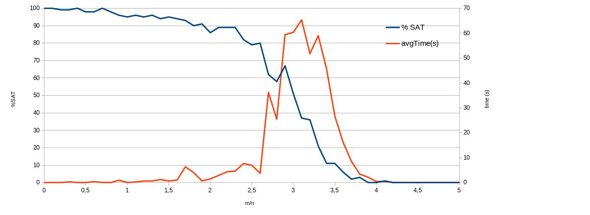
Figure 1: PSAT Phase Transition; each point was obtained by solving 100 instances of PSAT in the same class.

The existence of a second-order phase transition for all NP-complete problems was conjectured by [Cheeseman, Kanefsky, and TaylorCheeseman et al.1991], and it was demonstrated to hold for the SAT problem and related problems [Kautz and SelmanKautz and Selman1992, Gent and WalshGent and Walsh1994], which are problems that show an easy-hard-easy empirical complexity, with most instances in the easy parts. In particular, several algorithms for the PSAT problem have displayed such behavior [Finger and De BonaFinger and De Bona2011, Finger and De BonaFinger and De Bona2015], such as the one in [Finger and De BonaFinger and De Bona2015] presented in Figure 1.

Thus, the reduction from PCE-Coherence to PSAT in encouraging, specially when regarding classes $\mathrm{GNP}^{s}_{k}$, where such reduction is linear, because many of the resulting PSAT-instances are expected to be solved easily.

4.4 An algorithm for PCE-Extension

Let us turn to the PCE-Extension problem. Given a coherent observable game $\mathcal{G}$, our aim is to find the maximum and minimum observer’s probabilistic constraints for some action $\alpha$ maintaining coherence. In other words, we need to search among the NP-witnesses of $\mathcal{G}$ for some that maximizes and minimizes the constraints on $\alpha$. One might wonder whether there are polynomial time (additive) approximation algorithms for such problem, i.e., given a PCE-Extension instance consisting of $\mathcal{G}$ and $\alpha$ and a precision $\varepsilon>0$, whether there exist polynomial time algorithms which return $m$ and $M$ such that:

• $|\underline{P}(\alpha)-m|<\varepsilon$;

• $|\overline{P}(\alpha)-M|<\varepsilon$.

The next results show the answer is negative, unless a huge breakthrough in complexity theory is achieved. First we establish an auxiliary reduction: from a game $G=\langle{P,N,A,u}\rangle$, we build the game $G^{*}=\langle{P,N,A^{*},u^{*}}\rangle$, where $A^{*}_{1}=A_{1}\cup\{b\}$, with $b\notin A_{1}$, and $A^{*}_{i}=A_{i}$, for $i\in P\setminus\{1\}$. Profiles $a\in A\subset A^{*}$ remain with the same utilities $u^{*}_{i}(a)=u_{i}(a)$, for all $i\in P$, and new profiles $p_{b}=\langle{b,a_{2},\ldots,a_{n}}\rangle\in A^{*}$, have utilities $u^{*}_{1}(p_{b})=\max\{u_{1}(a^{\prime}_{1},a_{2},\ldots,a_{n})~{}|~{}a^{\prime}_{1}\in A_{1}\}$ and $u^{*}_{i}(p_{b})=\max\{u_{i}(a)~{}|~{}a\in A\}$, for $i\in P\setminus\{1\}$.

Lemma 1

Game $G^{*}$ may be built from a game $G$ in polynomial time and has the new pure Nash equilibria $p_{b}$ in addition to the ones $G$ already has. _□

Proof

Game $G^{*}$ may be built in polynomial time because for every partitioning set $\{\langle{x,a_{2},\ldots,a_{n}}\rangle~{}|~{}x\in A_{1}\}$ of action profiles of $G$, we may add one unique new action profile $p_{b}=\langle{b,a_{2},\ldots,a_{n}}\rangle$; then it is necessary to add to $G^{*}$ less new utility values than the description of $G$ already has. Let $a=\langle{a_{1},\ldots,a_{n}}\rangle\in A$ be an action profile. If $a$ is a pure Nash equilibrium of $G$, players in $P\setminus\{1\}$ cannot increase their utilities by choosing other action in $A^{*}_{i}$ and, if player $1$ were able to do so, it would have to be by choosing action $b$, then $u^{*}_{1}(b,a_{2},\ldots,a_{n})>u_{1}(a^{\prime}_{1},a_{2},\ldots,a_{n})$, for all $a^{\prime}_{1}\in A_{1}$, contradicting the definition of $u^{*}_{1}$. If $a$ is not a pure Nash equilibrium of $G$, all players can increase their utilities by choosing other actions in $A_{i}$. Then, all pure Nash equilibria in $G$ remains pure Nash equilibria in $G^{*}$. Finally, action profiles $p_{b}=\langle{b,a_{2},\ldots,a_{n}}\rangle$ are clearly pure Nash equilibria in $G^{*}$ and we have the result. _■

Theorem 4

Unless $P=NP$, there does not exist a polynomial time algorithm that approximates, to any precision $\varepsilon\in(0,\frac{1}{2})$, the expected value by the minimization version of PCE-Extension. _□

Proof

Deciding the existence of pure Nash equilibria for games in $\mathrm{GNP}_{k}$ is an NP-complete problem; let us reduce this problem to PCE-Extension. Given a game $G$, we consider the coherent observable game $\mathcal{G}=\langle{G^{*},\{P(a_{i})\geq 0\}}\rangle$, for some arbitrary $a_{i}\in A_{i}$, for $i\in P$, together with action $b$ as an instance of PCE-Extension. The reduction from $G$ to $\mathcal{G}$ may be computed in polynomial time by Lemma 1. Suppose there exists a polynomial time algorithm that approximates to precision $\varepsilon\in(0,\frac{1}{2})$ the expected value by the minimization version of PCE-Extension. If $G$ does not have any pure Nash equilibrium, all equilibria in $G^{*}$ are of the type $p_{b}=\langle{b,a_{2},\ldots,a_{n}}\rangle$, then $\underline{P}(b)=1$ and the supposed algorithm should return $m>1-\varepsilon>\frac{1}{2}$. On the other hand, if $G$ has some pure Nash equilibrium, $\underline{P}(b)=0$ and the supposed algorithm should return $m<0+\varepsilon<\frac{1}{2}$. Therefore, such algorithm decides an NP-complete problem in polynomial time and $P=NP$. _■

Theorem 5

Unless $P=NP$, there does not exist a polynomial time algorithm that approximates, to any precision $\varepsilon\in(0,\frac{1}{2})$, the expected value by the maximization version of PCE-Extension. _□

Proof

Deciding the existence of pure Nash equilibria for games in $\mathrm{GNP}_{k}$ is an NP-complete problem; let us reduce this problem to some instances of PCE-Extension. Given a game $G$, we consider the coherent observable game $\mathcal{G}=\langle{G^{*},\{P(a_{i})\geq 0\}}\rangle$, for some arbitrary $a_{i}\in A_{i}$, for $i\in P\setminus\{1\}$, together with all actions $a_{1}\in A_{1}$ as $|A_{1}|$ different instances of PCE-Extension. The reduction from $G$ to $\mathcal{G}$ may be computed in polynomial time by Lemma 1. Suppose there exists a polynomial time algorithm that approximates to precision $\varepsilon\in(0,\frac{1}{2})$ the expected value by the maximization version of PCE-Extension. If $G$ does not have any pure Nash equilibrium, all equilibria in $G^{*}$ are of type $p_{b}=\langle{b,a_{2},\ldots,a_{n}}\rangle$, then $\overline{P}(a_{1})=0$, for all $a_{1}\in A_{1}$, and the supposed algorithm should return $M<0+\varepsilon<\frac{1}{2}$, for all PCE-Extension instances concerning $a_{1}\in A_{1}$. On the other hand, if $G$ has some pure Nash equilibrium, $\overline{P}(a_{1})=1$, for some $a_{1}\in A_{1}$, and the supposed algorithm should return $M>1-\varepsilon>\frac{1}{2}$, for a particular PCE-Extension instance concerning some $a_{1}\in A_{1}$. Therefore, we are able to decide the existence of a pure Nash equilibrium in game $G$ by running the supposed algorithm $|A_{1}|$ times in the instances comprehending $\mathcal{G}$ and $a_{1}\in A_{1}$; $G$ has a pure Nash equilibrium, if it returns $M>\frac{1}{2}$ for some instance, and $G$ has no equilibrium otherwise. Such routine based on the supposed algorithm decides an NP-complete problem in polynomial time, hence $P=NP$. _■

In the following, by means of a simple application of the binary search algorithm, we are able to provide a deterministic procedure to solve PCE-Extension, which shows that its complexity burden is all due to PCE-Coherence. Given a precision $\varepsilon=2^{-k}$, we proceed by making a binary search through the binary representation of the possible constraints to $\alpha$, solving PCE-Coherence in each step. Algorithm 1 presents the procedure to solve the maximization version of PCE-Extension. We called $\mathit{PCECoherence(G,\Pi)}$ the process that decides a PCE-Coherence instance $\mathcal{G}=\langle{G,\Pi}\rangle$. An algorithm for solving the minimization version of PCE-Extension is easily adaptable from Algorithm 1.

Algorithm 1 PCE-Extension-BS: a PCE-Extension solver via Binary Search

Input: A coherent PCE-Coherence instance $\mathcal{G}=\langle{G,\Pi}\rangle$, an action $a_{i}\in A_{i}$, and a precision $\varepsilon>0$.

Output: Maximum $P(a_{i})$ value with precision $\varepsilon$.

1:  $k:=\lceil|\log\varepsilon|\rceil$;

2:  $j:=1$, $v_{min}:=0$, $v_{max}:=1$;

3:  if $\mathit{PCECoherence}(G,\Pi\cup\{P(a_{i})=1\})=\mathrm{Yes}$ then

4:     $v_{min}:=1$;

5:  else

6:     while $j\leq k$ do

7:        $v_{max}=v_{min}+\frac{1}{2^{j}}$;

8:        if $\mathit{PCECoherence}(G,\Pi\cup\{P(a_{i})\geq v_{max}\})=\mathrm{Yes}$ then

9:           $v_{min}:=v_{max}$;

10:        end if

11:        $j\!\!+\!\!+$;

12:     end while

13:  end if

14:  return  $v_{min}$;

For instance, suppose the goal is to find the maximum possible value for constraining $\alpha$: the first iteration consists of solving PCE-Coherence for $P(\alpha)=1$, if it is coherent, $\overline{P}(\alpha)=1$, if not, $\overline{P}(\alpha)=0$ with precision $2^{0}$=1. In case the former iteration was not coherent, the second iteration consists of solving PCE-Coherence for $P(\alpha)=0.5$, if it is coherent, $\overline{P}(\alpha)=0.5$, if not, $\overline{P}(\alpha)=0$, both cases with precision $2^{-1}=0.5$. One more iteration will give precision $2^{-2}=0.25$, and it consists of solving PCE-Coherence for $P(\alpha)=0.75$ in case the former iteration was coherent, or for $P(\alpha)=0.25$ in case it was not. The process continues until the desired precision is reached and it takes $|\log 2^{-k}|+1=k+1$ iterations to be completed.

Theorem 6

Given a precision $\varepsilon>0$, PCE-Extension can be obtained with $O(|\log\varepsilon|)$ iterations of PCE-Coherence. _□

Example 5

Suppose we have an observable game $\mathcal{G}_{3}=\langle{G_{2},\Pi_{3}}\rangle$ with $G_{2}$ as in Example 2 and $\Pi_{3}$ a set of PCE consisting only of $P(a^{2})=0.9$. In order to solve PCE-Extension for finding $\overline{P}(b^{2})$ with precision $2^{-6}$, it will be necessary to solve seven instances of PCE-Coherence in the form below.

$$\pi_{2}+\pi_{4}+\pi_{5} =0.9$$

$$\pi_{2}+\pi_{5} =p_{5}$$

$$\pi_{1}+\pi_{2}+\pi_{3}+\pi_{4}+\pi_{5} =1$$

$$\pi_{1},\pi_{2},\pi_{3},\pi_{4},\pi_{5} \geq 0$$

The necessary iterations of PCE-Coherence are displayed in Table 3. Our algorithm returns $\overline{P}(b^{2})\approx 0.890625$, which is accurate within precision $2^{-6}=0.015625$, since $\overline{P}(b^{2})=0.9$.

Iteration	$p_{5}$	$\pi^{\prime}$	Coherence
1	$1_{2}=1$	-	No
2	$0.1_{2}=0.5$	$[0.1,0.5,0,0.4,0]$	Yes
3	$0.11_{2}=0.75$	$[0.1,0.75,0,0.15,0]$	Yes
4	$0.111_{2}=0.875$	$[0.1,0.875,0,0.025,0]$	Yes
5	$0.1111_{2}=0.9375$	-	No
6	$0.11101_{2}=0.90625$	-	No
7	$0.111001_{2}=0.890625$	$[0.1,0.890625,0,0.009375,0]$	Yes

Table 3: Iterations for solving PCE-Extension in Example 5.

_□

5 Coherence allowing mixed equilibria

We proceed on studying PCE-Coherence with respect to the more general concept of mixed Nash equilibrium.

A mixed-strategy for player $i$ is a rational probability distribution $\sigma_{i}$ over the set $A_{i}$ of actions for player $i$, and $\Sigma=\Sigma_{1}\times\cdots\times\Sigma_{n}$ is the set of mixed-strategy profiles, in which each $\Sigma_{i}$ is the set of all possible mixed-strategies for player $i$. It is assumed that each player’s choice of strategy is independent from all other players’ choices, so the expected utility function $U_{i}$ for player $i$ is given by:

$$U_{i}(\sigma)=\sum_{a\in A}u_{i}(a)\prod_{j\in P}\sigma_{j}(a_{j}),$$

where $\sigma\in\Sigma$. A mixed-strategy profile $e=\langle{\sigma_{1},\ldots,\sigma_{i},\ldots,\sigma_{n}}\rangle$ is a mixed Nash equilibrium if, for every player $i$, $U_{i}(e)\geq U_{i}(\sigma_{1},\ldots,\sigma^{\prime}_{i},\ldots,\sigma_{n})$ for every $\sigma^{\prime}_{i}\in\Sigma$; each $\sigma_{i}$ in $e$ is called a best response for player $i$ given the other players mixed-strategies in $e$. Then, a mixed-strategy profile is a Nash equilibrium if, and only if, it is composed by best responses for all players. A game $G$ always has at least one mixed Nash equilibrium [NashNash1951].

Note that an action profile $a$ may be seen as a mixed-strategy profile $\sigma$ by taking each action $a_{i}\in a$ for player $i$ as the mixed-strategy $\sigma_{i}\in\sigma$ that assigns $1$ to $a_{i}$ and $0$ to the other actions in $A_{i}$. This way, $a$ is a pure Nash equilibrium if, and only if, its associated $\sigma$ is a mixed Nash equilibrium.

The mixed-strategy setting may be better understood if we think of a game situation that repeatedly occurs and, in each instance, the players choose their actions randomly according to their mixed-strategy.

In this context, an observable game is a game that repeatedly occurs and which is known to be at one of its (mixed) equilibria, but the external observer does not know exactly which one. An instance of the game will be played and the observer assigns subjective probabilities to actions being part of the action profile to be reached in that instance. Formally, an observable game is a pair $\mathcal{G}=\langle{G,\Pi}\rangle$ as before. We may again interpret these probability assignments as bets placed by the observer to the actions that the players are allowed to choose.

Another way of understanding observable games is by imagining there are many game situations with the same setting, and that repeatedly occurs, and all these game situations are at some mixed Nash equilibrium. With that knowledge, the external observer looks at one game situation that is about to have a new instance played, but he does not know exactly which game situation among the many ones existing this is. Then, the observer does not know which is the mixed Nash equilibrium the game situation he is looking at is in and he assigns subjective probabilities for the players’ actions being part of the action profile resulting from the game situation instance.

As before, we suppose that there is a probability distribution over the mixed-strategy equilibria. It is important to note that this probability distribution is independent from probability distribution in a mixed-strategy. The former probability distribution ranges over mixed-strategy equilibria and the latter ranges over actions. If $e_{j}=\langle{\sigma_{1j},\ldots,\sigma_{nj}}\rangle\in E_{G}$, $\sigma_{ij}$ designates the $i$-th component of $e_{j}$. In this setting, the probability function $P$ over mixed Nash equilibria induces the probability $P(a_{i})$ of an action $a_{i}$ by

$$P(a_{i})=\sum_{e_{j}\in E_{G}}\sigma_{ij}(a_{i})\cdot P(e_{j}).$$

The definition of probabilistic constraints on equilibria (PCE) is analogous to that in Section 2, namely a set of probability assignments on actions. PCE-Coherence is similarly defined as the problem of, given an observable game $\mathcal{G}=\langle{G,\Pi}\rangle$, deciding if it is coherent, i.e. deciding if there exists a probability function over the set of equilibria that satisfies all constraints in $\Pi$.

Example 6

Recall Example 1 where we had the game between Alice and Bob in which Alice’s actions were $a^{1}$, $a^{2}$, and $a^{3}$, and Bob’s actions were $b^{1}$, $b^{2}$, and $b^{3}$, such that the joint utilities are in Table 1. This game has three pure equilibria, now viewed as special cases of mixed equilibria: $e_{1}=\langle{\sigma_{1}^{1},\sigma_{2}^{1}}\rangle$, where $\sigma_{1}^{1}(a^{1})=1$, $\sigma_{1}^{1}(a^{2})=\sigma_{1}^{1}(a^{3})=0$, $\sigma_{2}^{1}(b^{1})=1$, $\sigma_{2}^{1}(b^{2})=\sigma_{2}^{1}(b^{3})=0$; and $e_{2}=\langle{\sigma_{1}^{2},\sigma_{2}^{2}}\rangle$ and $e_{3}=\langle{\sigma_{1}^{3},\sigma_{2}^{3}}\rangle$ that are also based on the ones described in Example 1. However, there are several other mixed equilibria among which we highlight $e_{4}=\langle{\sigma_{1}^{4},\sigma_{2}^{4}}\rangle$ given by

$$\sigma_{1}^{4}(a^{1})=\frac{2}{3},~{}~{}\sigma_{1}^{4}(a^{2})=\frac{1}{3},~{}~{}\sigma_{1}^{4}(a^{3})=0,~{}~{}~{}~{}~{}~{}\sigma_{2}^{4}(b^{1})=\frac{4}{5},~{}~{}\sigma_{2}^{4}(b^{2})=\frac{1}{5},~{}~{}\sigma_{2}^{4}(b^{3})=0.$$

We have established that if only pure equilibria are considered, the constraints $P(a^{2})=\frac{1}{3}$ and $P(b^{3})=\frac{1}{4}$ are incoherent. However, in a context that considers mixed Nash equilibria, they are coherent, as we detail in Example 7. _□

5.1 Complexity of PCE-Coherence over $\mathrm{2GNP}$

We also formulate PCE-Coherence in linear algebraic terms. Let $\Pi=\{P(\alpha_{i})\bowtie_{i}p_{i},1\leq i\leq K\}$ be a set of PCE for an observable game with $M$ mixed Nash equilibria. PCE-Coherence becomes the problem of deciding the existence of a vector $\pi$ satisfying

$$A\pi \bowtie p$$

$$\sum\pi_{j} = 1$$ (3)

$$\pi \geq 0$$

where $A=[a_{ij}]$ is a $K\times M$ matrix whose columns represent the mixed Nash equilibria in the game. In this case $a_{ij}=\sigma_{pj}(\alpha_{i})$, where $p\in P$ is such that $\alpha_{i}\in A_{p}$, that is $a_{ij}$ is the probability assignment of action $\alpha_{i}$ in the mixed equilibrium $e_{j}$ by player $p$. Again, we join the first two conditions in (3) in matrix $A$. In this setting, the existence of small witnesses for coherence given by Carathéodory’s Theorem also applies. This leads to a similar complexity result for PCE-Coherence as we have in Theorem 1.

Theorem 7

PCE-Coherence over a GNP-class is a problem in NP. _□

Proof

This proof is totally analogous to that of Theorem 1. Suppose the observable game $\mathcal{G}=\langle{G,\Pi}\rangle$ is coherent and $|\Pi|=K$. Therefore there exists a probability distribution $\pi$ over the set of all possible (mixed) Nash equilibria that satisfy $\Pi$. By the Carathéodory’s Theorem [EckhoffEckhoff1993] there is a probability distribution assigning non-zero probabilities to at most $K+1$ equilibria. These equilibria are polynomially bounded in size since $G$ is in a GNP-class. Therefore, there is a witness $\pi$ whose size is polynomially bounded attesting $\Pi$ is satisfied, so PCE-Coherence is in NP. _■

It is not known if there exists a non-deterministic polynomial algorithm that computes an exact mixed Nash equilibrium for games with at least $3$ players, and such a result would imply theoretical breakthroughs in complexity theory [Etessami and YannakakisEtessami and Yannakakis2010]. On the other hand, for games with $2$ players an algorithm whose complexity lies in NP has been described [PapadimitriouPapadimitriou2007]. Thus, restricting $\mathrm{GNP}_{k}$ to games with two players generates a GNP-class with respect to mixed Nash equilibrium, which we call $\mathrm{2GNP}$. Further, we actually have to restrict the equilibrium concept to “small” representations, as there are infinitely many mixed Nash equilibria for some games — i.e. the equilibria representation sizes will be polynomially bounded on the game parameters.

Note that both standard normal form and graphical normal form may be used to represent games in $\mathrm{2GNP}$. Also note that the restriction on “small” representations implies that each game has only finitely many mixed equilibria. The following proposition has a reduction from [Conitzer and SandholmConitzer and Sandholm2008] that we use for establishing the complexity of PCE-Coherence over $\mathrm{2GNP}$ and the inapproximability results later in this section.

Proposition 2 (Conitzer & Sandholm [Conitzer and SandholmConitzer and Sandholm2008])

Let $\varphi$ be a CNF Boolean formula with $n$ propositional variables. Then, there exists a $2$-player game $G_{\varphi}$ which may be built in polynomial time, with $f_{i}\in A_{i}$, for $i\in\{1,2\}$, such that $\varphi$ is satisfiable if, and only if, it has a mixed Nash equilibrium which is a mixed-strategy profile $\sigma_{SAT}=\langle{\sigma_{1},\sigma_{2}}\rangle$, where $\sigma_{1}$ assigns positive probability $\frac{1}{n}$ to $n$ distinct actions in $A_{1}\setminus\{f_{1}\}$. Furthermore, action profile $\sigma_{f}=\langle{f_{1},f_{2}}\rangle$ is the only other possible mixed Nash equilibrium in $G_{\varphi}$. _□

Theorem 8

PCE-Coherence over $\mathrm{2GNP}$ is NP-complete. _□

Proof

Membership in NP follows from Theorem 7. SAT is an NP-complete problem; let us reduce this problem to PCE-Coherence. Given a CNF Boolean formula $\varphi$, let $G_{\varphi}$ be the game in Proposition 2. We consider the instance $\mathcal{G}=\langle{G_{\varphi},\{P(f_{1})=0\}}\rangle$ of PCE-Coherence, which may be computed from $\varphi$ in polynomial time. $\mathcal{G}$ is coherent if, and only if, $G_{\varphi}$ has another mixed Nash equilibrium beyond $\sigma_{f}$, which happens if, and only if, $\varphi$ is satisfiable. Thus, PCE-Coherence over $\mathrm{2GNP}$ is NP-hard. _■

Example 7

We show the reduction of PCE-Coherence to the matrix form (3) for observable game in Example 6. We only show the columns of matrix $A$ corresponding to equilibria mentioned in Example 6, which already provides a model satisfying the set of PCE in vector $p$ below.

$$A\pi=\begin{array}[]{c}\phantom{c}\\ a^{1}\\ a^{2}\\ a^{3}\\ b^{1}\\ b^{2}\\ b^{3}\end{array}\left[\begin{array}[]{cccc}1&1&1&1\\ 1&0&0&\frac{2}{3}\\ 0&1&0&\frac{1}{3}\\ 0&0&1&0\\ 1&0&0&\frac{4}{5}\\ 0&0&0&\frac{1}{5}\\ 0&1&1&0\end{array}\right]\cdot\left[\begin{array}[]{c}\pi_{1}\\ \pi_{2}\\ \pi_{3}\\ \pi_{4}\end{array}\right]=\left[\begin{array}[]{c}1\\ p_{2}\\ \frac{1}{3}\\ p_{4}\\ p_{5}\\ p_{6}\\ \frac{1}{4}\end{array}\right]=p$$

This matrix system is solvable due to, for example, the vector $\pi=[\frac{1}{2},\frac{1}{4},0,\frac{1}{4}]^{\prime}$, so the PCE-Coherence instance is coherent. _□

The complexity results of Theorems 7 and 8 rely on non-deterministic algorithm. For a deterministic algorithm, the immediate possibilities are brute force (exponential) search or reduction to SAT (an NP-complete problem with very efficient implementations). However, it has been shown that, in the case of probabilistic reasoning, both approaches are far inferior to an approach combining linear algebraic and SAT methods [Finger and De BonaFinger and De Bona2011]. Thus, we provide a potentially more practical algorithm combining linear algebraic methods and game solvers whose equilibria can be efficiently determined.

5.2 A column generation algorithm for PCE-Coherence over $\mathrm{2GNP}$

An algorithm for solving PCE-Coherence has to provide a means to find a solution for Equation 3 if one exists and, otherwise, determine that no solution is possible. Without loss of generality we assume that the first line of matrix $A$ corresponds to the condition $\sum\pi_{i}=1$ and that the first position of vector $p$ is $1$ and the remaining positions are sorted in a decreasing order. Note that now matrix $A$ has $K+1$ rows.

Let $\overline{A}=[U_{K+1}|A]$ be the matrix $A$ prefixed with the $\{0,1\}$-upper diagonal square matrix $U_{K+1}$ of dimension $K+1$ in which the positions on the diagonal and above it are $1$ and all the other positions are $0$. Note that both $A$ and $\overline{A}$ can have an exponential number of columns $O(2^{K})$.

We now provide a method similar to PSAT-solving to deal with mixed equilibria. Note that in the case of pure equilibria the elements $a_{ij}$ could have values only $0$ and $1$, but now $a_{ij}=\sigma_{pj}(\alpha_{i})\in[0,1]$. Also note that the columns of $U_{K+1}$ may not all represent equilibria, so $\overline{A}$ has some columns that represent mixed equilibria and some that do not. We construct a vector $c$ of costs having the same size of matrix $\overline{A}$ such that $c_{j}\in\{0,1\}$, $c_{j}=0$ if column $\overline{A}^{j}$ represents a mixed equilibrium for game $G$. Then we generate the following optimization problem associated to (3).

$$\begin{array}[]{lll}\min&c^{\prime}\cdot\pi\\ \mbox{subject to}&\overline{A}\cdot\pi=p\\ &\pi\geq 0\end{array}$$ (7)

We actually solve the problems where all relations in vector $\bowtie$ in (3) are “$=$”. This standard form is convenient for using the already existing optimization methods; a formulation for the general case similar to (7) may be achieved by performing simple usual linear programming tricks [Bertsimas and TsitsiklisBertsimas and Tsitsiklis1997].

Lemma 2

Given a PCE-Coherence instance $\mathcal{G}=\langle{G,\Pi}\rangle$ and its associated linear algebraic restrictions (3), $\mathcal{G}$ is coherent if, and only if, minimization problem (7) has a minimum such that $c^{\prime}\pi=0$. _□

Condition $c^{\prime}\pi=0$ means that only the columns of $\overline{A}^{j}$ corresponding to actual mixed equilibria of the game $G$ can be attributed probability $\pi_{j}>0$, which immediately leads to solution of (7). Minimization problem (7) can be solved by an adaptation of the simplex method with column generation such that the columns of $A$ are generated on the fly. The simplex method is a stepwise method which at each step considers a basis $B$ consisting of $K+1$ columns of matrix $\overline{A}$ and computes its associated cost [Bertsimas and TsitsiklisBertsimas and Tsitsiklis1997]. The processing proceeds by finding a column of $\overline{A}$ outside $B$, creating a new basis by substituting one of the columns of $B$ by this new column such that the associated cost never increases. To guarantee the cost never increases, the new column $\overline{A}^{j}$ to be inserted in the basis has to obey a restriction called reduced cost given by $\tilde{c}_{j}=c_{j}-c_{B}B^{-1}A^{j}\leq 0$, where $c_{j}$ is the cost of column $A^{j}$, $B$ is the basis and $c_{B}$ is the cost associated to the basis. Note that in our case, we are only inserting columns that represent actual mixed equilibria, so that we only insert columns of matrix $A$ and their associated cost $c_{j}=0$. Therefore, every new column $A^{j}$ to be inserted in the basis $B$ has to obey the inequality

$$c_{B}B^{-1}A^{j}\geq 0.$$ (8)

A column $A^{j}$ representing a mixed Nash equilibrium may or may not satisfy condition (8). We call a mixed Nash equilibrium that does satisfy (8) as cost reducing mixed equilibrium. Our strategy for column generation is given by finding cost reducing mixed equilibrium for a given basis.

Lemma 3

There exists an algorithm that decides the existence of cost reducing mixed equilibrium whose complexity is in NP. _□

Proof

Since we are dealing with games whose mixed Nash equilibria can be computed in NP, we can guess one such equilibrium and in polynomial time both verify it is a Nash equilibrium for the game and that it satisfies Equation 8. _■

We can actually build a deterministic algorithm for Lemma 3 by reducing it to a SAT problem. In fact, computing equilibrium in $\mathrm{2GNP}$ can be encoded in a 3-SAT formula $\varphi$; the condition (8) can also be encoded by a 3-SAT formula $\psi$ in linear time, e.g. by Warners algorithm [WarnersWarners1998], such that the SAT problem consisting of deciding $\varphi\cup\psi$ is satisfiable if, and only, if there exists a cost reducing mixed equilibrium. Furthermore its valuation provides the desired column $A^{j}$. This SAT-based algorithm we call the PCE-Coherence Column Generation Method.

Algorithm 2 PCE-Coherence-CG: a PCE-Coherence solver via Column Generation

Input: A PCE-Coherence instance $\mathcal{G}=\langle{G,\Pi}\rangle$.

Output: No, if $\mathcal{G}$ is not coherent. Or a solution $\langle{B,\pi}\rangle$ that minimizes (7).

1:  $p:=[\{1\}\cup\{p_{i}~{}|~{}P(\alpha_{i})=p_{i}\in\Pi,1\leq i\leq K\}]$ in descending order;

2:  $B^{(0)}:=U_{K+1};$

3:  $s:=0$, $\pi^{(s)}=(B^{(0)})^{-1}\cdot p$ and $c^{(s)}=[c_{1}\cdots c_{K+1}]^{\prime};$

4:  while $c^{(s)}{}^{\prime}\cdot\pi^{(s)}\neq 0$ do

5:     $y^{(s)}=\mathit{GenerateColumn}(B^{(s)},G,c^{(s)});$

6:     if $y^{(s)}$ column generation failed then

7:        return  No;   {PCE-Coherence instance is unsatisfiable}

8:     else

9:        $B^{(s+1)}=\mathit{merge}(B^{(s)},y^{(s)});$

10:        $s\!\!+\!\!+$, recompute $\pi^{(s)}:=(B^{(s-1)})^{-1}\cdot p$; $c^{(s)}$ the costs of $B^{(s)}$ columns;

11:     end if

12:  end while

13:  return  $\langle{B^{(s)},\pi^{(s)}}\rangle$;   {PCE-Coherence instance is satisfiable}

Algorithm 2 presents the top level PCE-Coherence decision procedure. Lines 1–3 present the initialization of the algorithm. We assume the vector $p$ is in descending order. At the initial step we make $B^{(0)}=U_{K+1}$, this forces $\pi^{(0)}_{K+1}=p_{K+1}\geq 0$, $\pi^{(0)}_{j}=p_{j}-p_{j+1}\geq 0,1\leq j\leq K$; and $c^{(0)}=[c_{1}\cdots c_{K+1}]^{\prime}$, where $c_{j}=0$ if column $j$ in $B^{(0)}$ is a Nash equilibrium; otherwise $c_{j}=1$. Thus the initial state $s=0$ is a feasible solution.

Algorithm 2 main loop covers lines 4–12 which contains the column generation strategy at beginning of the loop (line 5). If column generation fails the process ends with failure in line 7; the correctness unsatisfiability by failure is guaranteed by Lemma 2. Otherwise a column is removed and the generated column is inserted in a process we called merge at line 9. The loop ends successfully when the objective function (total cost) $c^{(s)}{}^{\prime}\cdot\pi^{(s)}$ reaches zero and the algorithm outputs a probability distribution $\pi$ and the set of Nash equilibria columns in $B$, at line 13.

The procedure merge is part of the simplex method which guarantees that given a column $y$ and a feasible solution $\langle{B,\pi}\rangle$ there always exists a column $j$ in $B$ such that if $B[j:=y]$ is obtained from $B$ by replacing column $j$ with $y$, then there is $\tilde{\pi}\geq 0$ such that $\langle{B[j:=y],\tilde{\pi}}\rangle$ is a feasible solution. We have thus proved the following result.

Theorem 9

Algorithm 2 decides PCE-Coherence using column generation. _□

5.3 An algorithm for PCE-Extension over $\mathrm{2GNP}$

We now analyze PCE-Extension in analogy of what has been done in Section 4.2. The definition of PCE-Extension is analogous to that of the pure equilibrium case, i.e. given a coherent observable game $\mathcal{G}=\langle{G,\Pi}\rangle$, with $G$ in $\mathrm{2GNP}$, and an action $a_{i}\in A_{i}$, PCE-Extension consists in finding probability functions $\underline{P}$ and $\overline{P}$ that satisfy $\Pi$ such that $\underline{P}(a_{i})$ is minimal and $\overline{P}(a_{i})$ is maximal. As far as approximation algorithms are concerned for PCE-Extension, we have analogous results to Theorems 4 and 5.

Theorem 10

Unless $P=NP$, there does not exist a polynomial time algorithm that approximates, to any precision $\varepsilon\in(0,\frac{1}{2})$, the expected value by the minimization version of PCE-Extension. _□

Proof

SAT is an NP-complete problem; let us reduce this problem to PCE-Extension. Given a CNF Boolean formula $\varphi$, let $G_{\varphi}$ be the game in Proposition 2. We consider the coherent observable game $\mathcal{G}=\langle{G_{\varphi},\{P(a_{i})\geq 0\}}\rangle$, for some arbitrary $a_{i}\in A_{i}$, for $i\in P$, together with action $f_{1}$ as an instance of PCE-Extension. The reduction from $\varphi$ to $\mathcal{G}$ may be computed in polynomial time. Suppose there exists a polynomial time algorithm that approximates to precision $\varepsilon\in(0,\frac{1}{2})$ the expected value by the minimization version of PCE-Extension. If $\varphi$ is not satisfiable, the only equilibrium in $G_{\varphi}$ is $\sigma_{f}$, then $\underline{P}(f_{1})=1$ and the supposed algorithm should return $m>1-\varepsilon>\frac{1}{2}$. On the other hand, if $\varphi$ is satisfiable, $\underline{P}(f_{1})=0$ and the supposed algorithm should return $m<0+\varepsilon<\frac{1}{2}$. Therefore, such algorithm decides an NP-complete problem in polynomial time and $P=NP$. _■

Theorem 11

Unless $P=NP$, there does not exist a polynomial time algorithm that approximates, to any precision $\varepsilon\in(0,\frac{1}{6})$, the expected value by the maximization version of PCE-Extension. _□

Proof

SAT is an NP-complete problem; let us reduce this problem to PCE-Extension. Given a CNF Boolean formula $\varphi$, let $G_{\varphi}$ be the game in Proposition 2. We consider the coherent observable game $\mathcal{G}=\langle{G_{\varphi},\{P(a_{2})\geq 0\}}\rangle$, for some arbitrary $a_{2}\in A_{2}$, together with some arbitrary action $a_{1}\in A_{1}\setminus\{f_{1}\}$ as an instance of PCE-Extension. The reduction from $\varphi$ to $\mathcal{G}$ may be computed in polynomial time. Suppose there exists a polynomial time algorithm that approximates to precision $\varepsilon\in(0,\frac{1}{6})$ the expected value by the maximization version of PCE-Extension. If $\varphi$ is not satisfiable, the only equilibrium in $G_{\varphi}$ is $\sigma_{f}$, then $\overline{P}(a_{1})=0$ and the supposed algorithm should return $M<0+\varepsilon<\frac{1}{6}$. On the other hand, if $\varphi$ is satisfiable, $\overline{P}(a_{1})=\frac{1}{3}$ and the supposed algorithm should return $M>\frac{1}{3}-\varepsilon>\frac{1}{6}$. Therefore, such algorithm decides an NP-complete problem in polynomial time, hence $P=NP$. _■

PCE-Extension in the mixed equilibrium setting may also be solved by Algorithm 1 with $\mathit{PCECoherence(G,\Pi)}$ now being a process by Algorithm 2. We have a similar result as in Theorem 6.

Theorem 12

Given an instance of PCE-Extension over $\mathrm{2GNP}$ and a precision $\varepsilon>0$, PCE-Extension can be obtained with $O(|\log\varepsilon|)$ iterations of PCE-Coherence. _□

6 Related work

The framework defined in Section 3, where probabilities are assigned to pure Nash equilibria, is very similar to another concept of equilibrium: the correlated equilibrium [AumannAumann1974]. A correlated equilibrium in a game $G=\langle{P,N,A,u}\rangle$ is a probability distribution over the set of action profiles $A$ that satisfies a specific equilibrium property. Despite the similarity, these are distinct objects: while our framework models the uncertainty about which pure Nash equilibrium will be reached in a game (by a probability distribution over $E_{G}\subset A$), the distribution in a correlated equilibrium is the very concept of equilibrium and is defined over all possible action profiles (not necessarily Nash equilibria).

In a deeper comparison, for both computing a correlated equilibrium and deciding on the coherence of an observable game allowing only pure equilibria, it is necessary to guarantee that a probability distribution on action profiles satisfies some linear inequalities that model the equilibrium property, in the case of correlated equilibrium, and that represents the probabilistic constraints, in the case of coherence. However, while the correlated equilibrium inequalities may be directly derived from the given game [Papadimitriou and RoughgardenPapadimitriou and Roughgarden2008], in order to write the coherence inequalities, it is necessary to compute the Nash equilibria of the game, since the distribution in question is over such equilibria. This difference should explain the discrepancy in complexity between the problem of computing a correlated equilibrium, which is polynomial [Papadimitriou and RoughgardenPapadimitriou and Roughgarden2008], and that of computing a distribution over $E_{G}$ satisfying a set of PCE, which is non-deterministic polynomial; indeed, the proof we provide for the NP-completeness of PCE-Coherence (concerning only pure equilibria) depends on the NP-completeness of computing Nash equilibria.

Now, turning to PCE-Coherence allowing mixed Nash equilibria, there are many results stating that deciding on the existence of mixed equilibria in $2$-player games with some property, such as uniqueness, Pareto-optimality, etc, are NP-complete problems [Gilboa and ZemelGilboa and Zemel1989, Conitzer and SandholmConitzer and Sandholm2008]. PCE-Coherence may be seen as an addition to this list by Theorem 8 in Section 5 if one glimpses it as the problem of deciding whether there are at most $K+1$ mixed equilibria for which there is an associated vector $\pi$ that satisfies conditions in (3).

7 Conclusions and future work

By means of observable games, we have modeled the scenario of uncertainty about exactly what equilibrium is to be reached in a situation that will certainly reach one. To avoid the possible hardness of computing and enumerating all equilibria in order to assign probabilities to them, the proposed model instead allows the observer to assign probabilities to the possible actions of the players involved. PCE-Coherence over GNP-classes in the pure equilibrium case have been shown to be in NP, and to be NP-complete over NP-complete GNP-classes. We have also provided reductions of PCE-Coherence to PSAT, and of PCE-Extension to PCE-Coherence.

Let us resume the analogy between the study of equilibrium concepts and coherent observable games by highlighting that equilibrium computation is part of an ongoing utility debate [Papadimitriou and RoughgardenPapadimitriou and Roughgarden2008]. Since by the aspect of the model per se, an equilibrium concept explains agents behavior, the actual computation of an equilibrium might be regarded as completely irrelevant. Nevertheless, it might also be argued that it is only reasonable to accept that agents behave according to an equilibrium if it is not too hard to compute such equilibrium. In light of this discussion, we may conclude that the hardness results concerning PCE-Coherence point to the difficulty of the observer in being coherent; thus, it may explain failures in the management by local producers when competing with oligopolists.

However, PSAT has been shown to have an easy-hard-easy phase-transition, which means that possibly most cases of PSAT-instances resulting from the reduction from PCE-Coherence over pure equilibria can be solved easily. By this hypotheses, providing that the reduction itself is not too complex (as in the case of classes $\mathrm{GNP}^{s}_{k}$), in most cases it is not difficult for an observer to be coherent and then the responsibility for a poor management falls entirely over the poor knowledge on the oligopolistic market by the local producer.

Moreover, we believe that the framework of observable games we set in this work is in the interest of an observer who actually wants to compute the coherence and the extension of his probabilities over actions which are in equilibrium, independently of whether this equilibrium was actually computed or how it was established, e.g. again the local producer observing an oligopolistic market. In this way, beyond the reduction from PCE-Coherence to PSAT being encouraging due to the phase transition behavior of PSAT, the improvement in the technologies for implementing linear algebraic solvers and SAT, MAXSAT, and SMT solvers points out that these problems can now be dealt by practical applications in most cases.

For the mixed Nash equilibrium, the possibility of having a general PCE-Coherence solver lies on very improbable breakthrough in algorithms. However in 2-player games we are in the same zone as for general pure equilibrium PCE-Coherence problem; since it is NP-complete, most instances are expected to be easily solved in practice.

Finally, we highlight that the optimistic perspectives for solving in practice the problems proposed in this work also justify the uncertainty model that was designed to avoid the need to establish a probability distribution over all equilibria in a game. Solving these problems, of course, involves computing some equilibria, however, our conclusions point out that, in most cases, only a few equilibria need to be computed.

For the future, besides tackling some practical problems and implementations, the techniques here presented can be expanded to other forms of equilibrium such as $\varepsilon$-Nash equilibrium [Daskalakis, Goldberg, and PapadimitriouDaskalakis et al.2009].

Funding

This study was financed in part by the Coordenação de Aperfeiçoamento de Pessoal de Nível Superior - Brasil (CAPES) - Finance Code 001. Eduardo Fermé was partially supported by NOVA LINCS (UIDB/04516/2020) with the financial support of FCT - Fundação para a Ciência e a Tecnologia, through national funds and FCT MCTES IC&DT Project - AAC 02/SAICT/2017. Marcelo Finger was partly supported by Fapesp projects 2019/07665-4, 2015/21880-4 and 2014/12236-1 and CNPq grant PQ 303609/2018-4.

References

- [\citeauthoryearAumannAumann1974] Aumann, R. J. (1974). Subjectivity and correlation in randomized strategies. Journal of Mathematical Economics 1(1), 67–96.
- [\citeauthoryearBertsimas and TsitsiklisBertsimas and Tsitsiklis1997] Bertsimas, D. and J. Tsitsiklis (1997). Introduction to Linear Optimization. Athena Scientific series in optimization and neural computation. Athena Scientific.
- [\citeauthoryearCheeseman, Kanefsky, and TaylorCheeseman et al.1991] Cheeseman, P., B. Kanefsky, and W. M. Taylor (1991). Where the really hard problems are. In 12th IJCAI, pp. 331–337. Morgan Kaufmann.
- [\citeauthoryearConitzer and SandholmConitzer and Sandholm2008] Conitzer, V. and T. Sandholm (2008). New complexity results about Nash equilibria. Games and Economic Behavior 63(2), 621–641.
- [\citeauthoryearCookCook1971] Cook, S. A. (1971). The complexity of theorem-proving procedures. In Conference Record of Third Annual ACM Symposium on Theory of Computing (STOC), pp. 151–158. ACM.
- [\citeauthoryearDaskalakis, Goldberg, and PapadimitriouDaskalakis et al.2009] Daskalakis, C., P. W. Goldberg, and C. H. Papadimitriou (2009). The complexity of computing a Nash equilibrium. SIAM Journal on Computing 39(1), 195–259.
- [\citeauthoryearde Finettide Finetti1931] de Finetti, B. (1931). Sul significato soggettivo della probabilità. Fundamenta Mathematicae 17(1), 298–329. Translated into English as “On the Subjective Meaning of Probability”, In: P. Monari and D. Cocchi (Eds.), Probabilità e Induzione, Clueb, Bologna, 291-321, 1993.
- [\citeauthoryearde Finettide Finetti2017] de Finetti, B. (2017). Theory of probability: A critical introductory treatment. John Wiley & Sons. Translated by Antonio Machí and Adrian Smith.
- [\citeauthoryearEckhoffEckhoff1993] Eckhoff, J. (1993). Helly, Radon, and Caratheodory type theorems. In P. M. Gruber and J. M. Wills (Eds.), Handbook of Convex Geometry, pp. 389–448. Elsevier Science Publishers.
- [\citeauthoryearEtessami and YannakakisEtessami and Yannakakis2010] Etessami, K. and M. Yannakakis (2010). On the complexity of Nash equilibria and other fixed points. SIAM Journal on Computing 39(6), 2531–2597.
- [\citeauthoryearFinger and De BonaFinger and De Bona2011] Finger, M. and G. De Bona (2011). Probabilistic satisfiability: Logic-based algorithms and phase transition. In T. Walsh (Ed.), IJCAI, pp. 528–533. IJCAI/AAAI.
- [\citeauthoryearFinger and De BonaFinger and De Bona2015] Finger, M. and G. De Bona (2015). Probabilistic satisfiability: algorithms with the presence and absence of a phase transition. Annals of Mathematics and Artificial Intelligence 75(3), 351–379.
- [\citeauthoryearFischer, Holzer, and KatzenbeisserFischer et al.2006] Fischer, F., M. Holzer, and S. Katzenbeisser (2006). The influence of neighbourhood and choice on the complexity of finding pure Nash equilibria. Information Processing Letters 99(6), 239–245.
- [\citeauthoryearGent and WalshGent and Walsh1994] Gent, I. P. and T. Walsh (1994). The SAT phase transition. In ECAI94 – Proceedings of the Eleventh European Conference on Artificial Intelligence, pp. 105–109. John Wiley & Sons.
- [\citeauthoryearGeorgakopoulos, Kavvadias, and PapadimitriouGeorgakopoulos et al.1988] Georgakopoulos, G., D. Kavvadias, and C. H. Papadimitriou (1988). Probabilistic satisfiability. Journal of Complexity 4(1), 1–11.
- [\citeauthoryearGilboa and ZemelGilboa and Zemel1989] Gilboa, I. and E. Zemel (1989). Nash and correlated equilibria: Some complexity considerations. Games and Economic Behavior 1(1), 80–93.
- [\citeauthoryearGottlob, Greco, and ScarcelloGottlob et al.2005] Gottlob, G., G. Greco, and F. Scarcello (2005). Pure Nash equilibria: Hard and easy games. Journal of Artificial Intelligence Research 24, 357–406.
- [\citeauthoryearHansen and JaumardHansen and Jaumard2000] Hansen, P. and B. Jaumard (2000). Probabilistic satisfiability. In Handbook of Defeasible Reasoning and Uncertainty Management Systems. Vol.5, pp. 321. Springer Netherlands.
- [\citeauthoryearKautz and SelmanKautz and Selman1992] Kautz, H. A. and B. Selman (1992). Planning as satisfiability. In ECAI, pp. 359–363.
- [\citeauthoryearNashNash1951] Nash, J. (1951). Non-cooperative games. Annals of Mathematics 54(2), 286–295.
- [\citeauthoryearNashNash1950a] Nash, J. F. (1950a). Equilibrium points in n-person games. Proceedings of the National Academy of Sciences 36(1), 48–49.
- [\citeauthoryearNashNash1950b] Nash, J. F. (1950b). Non-Cooperative Games. Ph. D. thesis, Princeton University.
- [\citeauthoryearNilssonNilsson1986] Nilsson, N. (1986). Probabilistic logic. Artificial Intelligence 28(1), 71–87.
- [\citeauthoryearPapadimitriouPapadimitriou2007] Papadimitriou, C. H. (2007). The complexity of finding Nash equilibria. In N. Nisan, T. Roughgarden, E. Tardos, and V. V. Vazirani (Eds.), Algorithmic game theory, pp. 29–51. Cambridge University Press.
- [\citeauthoryearPapadimitriou and RoughgardenPapadimitriou and Roughgarden2008] Papadimitriou, C. H. and T. Roughgarden (2008). Computing correlated equilibria in multi-player games. Journal of the ACM 55(3), 1–29.
- [\citeauthoryearWarnersWarners1998] Warners, J. P. (1998). A linear-time transformation of linear inequalities into conjunctive normal form. Inf. Process. Lett. 68(2), 63–69.