Polymers critical point originates Brownian non-Gaussian diffusion

Abstract

We demonstrate that size fluctuations close to polymers critical point originate the non-Gaussian diffusion of their center of mass. Static universal exponents $\gamma$ and $\nu$ – depending on the polymer topology, on the dimension of the embedding space, and on equilibrium phase – concur to determine the potential divergency of a dynamic response, epitomized by the center of mass kurtosis. Prospects in experiments and stochastic modeling brought about by this result are briefly outlined.

As a consequence of the central limit theorem, ordinary diffusive motion of mesoscopic particles in solution is characterized by a Gaussian probability density function (PDF) whose variance grows linearly over time. Numerous experiments performed in complex contexts Wang et al. (2009, 2012); Toyota et al. (2011); Chakraborty and Roichman (2020); Weeks et al. (2000); Wagner et al. (2017); Jeon et al. (2016); Yamamoto et al. (2017); Stylianidou et al. (2014); Parry et al. (2014); Munder et al. (2016); Cherstvy et al. (2018); Li et al. (2019); Cuetos et al. (2018); Hapca et al. (2008); Pastore et al. (2021), while confirming the linear temporal increase of the variance, highlight however distinct stages during which the PDF of the random motion is non-Gaussian. This interesting contingency has been called “Brownian non-Gaussian diffusion” and has inspired various mesoscopic approaches, invoking superposition of statistics Beck and Cohen (2003); Beck (2006); Hapca et al. (2008); Wang et al. (2012), diffusing diffusivities Chubynsky and Slater (2014); Chechkin et al. (2017); Jain and Sebastian (2017); Tyagi and Cherayil (2017); Miyaguchi (2017); Sposini et al. (2018a, b); Miotto et al. (2021), subordination concepts Chechkin et al. (2017), continuous time random walk Barkai and Burov (2020), and diffusion in disordered environments Pacheco-Pozo and Sokolov (2021), but presently few attempts have been made to establish a microscopic foundation of this phenomenon Baldovin et al. (2019); Hidalgo-Soria and Barkai (2020). To breach the central limit theorem Feller (1968) one possibility is the emergence of strong correlations; here we demonstrate that the polymers critical point, separating the dilute to the dense phase in the grand canonical ensemble de Gennes (1972, 1979); Vanderzande (1998); Madras and Slade (2013), indeed originates a Brownian yet non-Gaussian diffusion for the center of mass (CM) of a polymer in solution. Prospects in experiments and stochastic modeling brought about by this result are briefly outlined.

Consider the grand canonical description of an isolated polymer in solution in contact with a monomer chemostat. The size of the polymer $N$ is a random variable and to the event $N=n\in\mathbb{N}$ is associated an equilibrium distribution $P^{\star}_{N}(n)$ determined by the monomer fugacity $z$. Close to criticality $z\to z_{\mathrm{c}}^{-}$ the partition function asymptotically behaves as

$$Z_{\mathrm{gc}}(z)=\sum_{n}(\mu_{\mathrm{c}}\,z)^{n}\;n^{\gamma-1}\sim\left\{\begin{array}[]{ll}(1-z/z_{\mathrm{c}})^{-\gamma}&(\gamma>0)\\ -\ln(1-z/z_{\mathrm{c}})&(\gamma=0)\,,\\ \textrm{finite}&(\gamma<0)\end{array}\right.$$ (1)

where $\mu_{\mathrm{c}}$ is the (model-dependent) connective constant and $z_{\mathrm{c}}=\mu_{\mathrm{c}}^{-1}$. The entropic exponent $\gamma$ is specified by the space dimension $d$ and by the topology of the polymeric structure (homeomorphism type of the underlying graph); together with the metric exponent $\nu>0$ it identifies the universality class of the critical behavior. For the wide class of polymer networks in good solvent conditions, with any prescribed fixed topology $\mathcal{G}$ made of chains of equal lengths, this exponent is known thanks to the mapping with the magnetic $O(n\to 0)$ model de Gennes (1979) through the relation Duplantier (1989)

$$\gamma=\gamma_{\mathcal{G}}=1-\nu\,d\,\mathcal{L}+\sum_{L\geq 1}n_{L}\,\sigma_{L}\,,$$ (2)

where $\mathcal{L}$ is the number of physical loops (or cyclomatic number) in the polymer network, $n_{L}$ the number of vertices with functionality $L$, and $\sigma_{L}$ the associated scaling dimension (see Fig. 1 for examples and further details). Also in the case when monomers functionality is free to fluctuate as in lattice animals and trees Lubensky and Isaacson (1979); Vanderzande (1998), the $\gamma$ exponent can be exactly computed by relating the critical behavior of these systems to the Yang-Lee singularity of an Ising model in $d-2$ dimensions Parisi and Sourlas (1981); Brydges and Imbrie (2003) (again, more details in Fig. 1). The metric exponent characterizes the large $N$ behavior of the average square end-to-end distance of large polymer chains: $R^{2}\sim N^{2\nu}$. Unlike the entropic one, its value does not depend on topology (if fixed) but on the dimension of the embedding space (see Fig. 1). Note that both exponents can further depend on the polymer being in different equilibrium phases such as those triggered by monomer-monomer attractions (coil to globule transition) or by effective interactions with impenetrable surfaces (adsorption transition) de Gennes (1972); Vanderzande (1998).

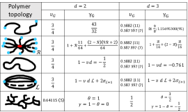
Figure 1: Metric and entropic exponents of different polymer network topologies (i.e. homeomorphism types) in $d=2$ and $d=3$ under good solvent conditions. First row refers to linear self-avoiding polymers: values in $d=2$ are exact and were first computed via Coulomb gas Nienhuis (1982); $d=3$ values have been originally obtained by Wilson-Fisher expansion in dimension $d=\epsilon-4$ for the $\varphi^{4}$ field theory of the $O(n\to 0)$ model with $\epsilon=1$ Guida and Zinn-Justin (1998) (first number), and later estimated with high precision Monte Carlo simulations Clisby (2010, 2017) (second number). Exponents from second to fourth row refer to star polymers with ${\mathcal{R}}$ arms Duplantier (1989), ring polymers, and watermelon graphs with ${\mathcal{L}}$ independent loops Duplantier (1989), respectively. Since topology is kept fixed, the $\nu$ exponent does not vary with respect to the linear case. The $\gamma$ exponent is obtained filling proper values for $\nu$, $d$, $\mathcal{L}$, $n_{L}$ in Eq. (2), together with $\sigma_{L}=(2-L)(9L+2)/64$ (exact, $d=2$) or $\sigma_{L}=\epsilon(2-L)L/16+O(\epsilon^{2})$ ($d=3$). For instance, with star polymers one has ${\mathcal{L}}=0$, $n_{1}={\mathcal{R}}$, and $n_{{\mathcal{R}}}=1$ (the $n_{2}$ monomers with functionality $L=2$ do not contribute as $\sigma_{2}=0$) – note that the $2$-arms topology ($n_{1}=2$, ${\mathcal{R}}=2$) corresponds to linear polymer. Similarly, with watermelon graphs ${\mathcal{L}}\geq 1$, $n_{{\mathcal{L}}+1}=2$. The last row refers instead to lattice animals, i.e. polymers in which the number of loops and branches can vary. In this case critical exponents in $d$ dimensions are related to the Lee-Yang edge singularity Parisi and Sourlas (1981) through the relations $\nu_{d+2}=(\beta_{d}+1)/2$ and $\theta_{d+2}=\beta_{d}+2$, where $\beta_{d}$ is the exponent controlling magnetization near the edge singularity. As the latter is exactly solvable in $d=0$ and $d=1$ with $\beta_{0}=-1$ and $\beta_{1}=-1/2$, respectively, one gets $\gamma_{2}=1-\theta_{2}=0$, $\gamma_{3}=1-\theta_{3}=-1/2$, and $\nu_{3}=3/2$. The exact expression for $\nu_{d+2}$ however breaks down with $d=0$ and for $\nu_{2}$ one has to rely on numerical estimates Jensen (2001), such as the one reported in table. Note that with $d\geq 3$ exponents $\gamma$ and $\nu$ are not independent but follow the relation $\gamma=1-(d-2)\nu$.

The position of the polymer CM $\bm{R}_{\mathrm{CM}}(t)=(X_{\mathrm{CM}}(t),Y_{\mathrm{CM}}(t),Z_{\mathrm{CM}}(t))$ undergoes a Brownian motion described by not (a)

$$\mathrm{d}\bm{R}_{\mathrm{CM}}(t)=\sqrt{2D(N(t))}\,\mathrm{d}\bm{B}(\mathrm{d}t)\,,$$ (3)

where $\bm{B}(t)$ is a Wiener process (Brownian motion). In view of the Stokes-Einstein relation Doi and F (1992); Yamamoto et al. (2021); not (b)

$$D(N)\sim D_{0}/N^{\nu}\,,$$ (4)

with $D_{0}$ specific of the polymer subunits. Under the present assumptions $D$ fluctuates with the polymer size: we see that $\bm{R}_{\mathrm{CM}}(t)$ becomes thus a subordinated stochastic process Feller (1968) conditioned by the history $[n(t)]\equiv\{n(t^{\prime})\in\mathbb{N}\;|\;0\leq t^{\prime}\leq t\}$ of the polymer size. It is convenient to reparametrize the diffusion path in terms of the coordinate $s\geq 0$, $\mathrm{d}s=2\,D(n(t))\,\mathrm{d}t$, corresponding to the realization of the stochastic process

$$S(t)\equiv 2\int_{0}^{t}\mathrm{d}t^{\prime}\,D(N(t^{\prime}))=2D_{0}\int_{0}^{t}\mathrm{d}t^{\prime}\,N^{-\nu}(t^{\prime})\,.$$ (5)

By using the subordination formula Feller (1968); Bochner (2020)

$$p_{\bm{R}_{\mathrm{CM}}}(\bm{r},t|n_{0};\bm{0})=\int_{0}^{\infty}\mathrm{d}s\,\dfrac{\mathrm{e}^{-\frac{\bm{r}^{2}}{2s}}}{(2\pi\,s)^{3/2}}\;p_{S}(s,t|n_{0})\,,$$ (6)

where $p_{\bm{R}_{\mathrm{CM}}}(\bm{r},t|n_{0};\bm{0})$ is the CM conditional PDF given the initial condition $p_{\bm{R}_{\mathrm{CM}}}(\bm{r},0|n_{0};\bm{0})=\delta_{n,n_{0}}\,\delta(\bm{r})$, moments of the subordinated process are straightforwardly connected to those of the subordinator. For instance, assuming an equilibrium distribution $P^{\star}_{N}(n_{0})$ for the initial size,

$$\mathbb{E}[X_{\mathrm{CM}}^{2}(t)]=\mathbb{E}[S(t)],\quad\mathbb{E}[X_{\mathrm{CM}}^{4}(t)]=3\,\mathbb{E}[S^{2}(t)]\,.$$ (7)

We already appreciate the influence of $\gamma$ and $\nu$ in these moments: while the latter enters in the definition of $S(t)$, the former characterizes $P^{\star}_{N}(n)$.

Importantly, the equilibrium distribution $P^{\star}_{N}(n)$ can be related to a simple master equation describing the polymerization/depolymerization process occurring as monomers add and detach to the polymer in the grand canonical ensemble. First of all we observe that if $n_{\mathrm{min}}$ is the minimal polymer size, through the change of variable $n\mapsto n-(n_{\mathrm{min}}-1)$ we can always associate the support $1\leq n<\infty$ to $P^{\star}_{N}(n)$ without altering the asymptotic behavior in Eq. (4). Regard then the (forward) master equation

$$\partial_{t}P_{N}(n,t|n_{0})=\mu\,P_{N}(n+1,t|n_{0})\quad\;\;(n>1)$$ (8)

$$\;\;\;+\lambda(n-1)\,P_{N}(n-1,t|n_{0})-(\mu+\lambda(n))\,P_{N}(n,t|n_{0})\,$$

$$\partial_{t}P_{N}(1,t|n_{0})=\mu\,P_{N}(2,t|n_{0})-\lambda(1)\,P_{N}(1,t|n_{0})\,.$$

Here $P_{N}(n,t|n_{0})$ is the probability for $N=n$ at time $t\geq 0$ given $N=n_{0}$ at $t=0$, and $\lambda(n)$, $\mu$ are the rates for association and dissociation, respectively. Defining the growth factor as $g(n)\equiv\lambda(n)/\mu$, it is straightforward to prove that stationarity is attained under detailed balance, $g(n)=P^{\star}_{N}(n+1)/P^{\star}_{N}(n)=\mu_{\mathrm{c}}z\,[(n+1)/n]^{\gamma-1}$: this identifies the polymerization process, given $P^{\star}_{N}(n)$. In chain polymerization Odian (2004), while it is natural to consider dissociation to be independent of the polymer size, aggregation is instead influenced by the ratio of the number of available configurations at sizes $n+1$ and $n$. This is the reason of the size-dependency $\lambda(n)$ assumed here, which is conveyed by the entropic correction $\propto n^{\gamma-1}$ outside the mean-field limit ($\gamma\neq 1$). Note that the rate $\mu$ remains a free parameter which may rescale Eq. (8), thus determining the time scale $\tau$ for the autocorrelation of $N(t)$. This is particularly apparent in the mean-field case ($\gamma=1$), where an elegant connection with the $M/M/1$ model (Markovian interarrival times/Markovian service times/1 server) in queuing theory Jain et al. (2007) allows to extend the identification even outside criticality and to analytically solve both the equilibrium and the out-of-equilibrium behavior Nampoothiri et al. (2021). The asymptotic behavior for small and large time of $P_{N}(n,t|n_{0})$ is $P_{N}(n,t|n_{0})\begin{subarray}{c}\sim\\ t\ll\tau\end{subarray}\delta_{n,n_{0}}$, $P_{N}(n,t|n_{0})\begin{subarray}{c}\sim\\ t\gg\tau\end{subarray}P^{\star}_{N}(n)$, respectively.

The equilibrium size distribution is directly deduced from the grand canonical partition function (generating function). Close to the critical point $z_{\mathrm{c}}=1/\mu_{\mathrm{c}}$ we may neglect regular contributions, and, remembering the definition of polylogarithm functions, $\mathrm{Li}_{s}(z)\equiv\sum_{n=1}^{\infty}z^{n}/n^{s}$ (which are finite in $z=1$ if $s>1$), we have

$$P^{\star}_{N}(n) = \dfrac{(z/z_{\mathrm{c}})^{n}}{n^{1-\gamma}\;\mathrm{Li}_{1-\gamma}(z/z_{\mathrm{c}})}$$ (12)

$$\sim \left\{\begin{array}[]{ll}\dfrac{(1-z/z_{\mathrm{c}})^{\gamma}\;(z/z_{\mathrm{c}})^{n}}{n^{1-\gamma}\;\Gamma(\gamma)}&(\gamma>0)\\ -\dfrac{(z/z_{\mathrm{c}})^{n}}{n\,\ln(1-z/z_{\mathrm{c}})}&(\gamma=0)\,.\\ \dfrac{(z/z_{\mathrm{c}})^{n}}{n^{1-\gamma}\,\mathrm{Li}_{1-\gamma}(z/z_{\mathrm{c}})}&(\gamma<0)\end{array}\right.$$

We are now in a position to evaluate expected values in Eq. (7). Let us primarily note that, with equilibrium initial conditions $P^{\star}_{N}(n_{0})$,

$$\begin{array}[]{ll}\mathbb{E}[S(t)]&\sim 2D_{0}\displaystyle\int_{0}^{t}\mathrm{d}t^{\prime}\sum_{n,n_{0}}\dfrac{P_{N}(n,t^{\prime}|n_{0})\,P^{\star}_{N}(n_{0})}{n^{\nu}}\\ &=2D_{0}\,t\,\mathbb{E}[N^{-\nu}]\,,\end{array}$$ (13)

where we have used the stationarity of $P^{\star}_{N}(n)$. Together with Eq. (7), this proves the Brownian character of the CM diffusion in equilibrium. Transients may display either sub- or super-diffusive stages, depending on the specific initial condition Nampoothiri et al. (2021). Using the asymptotic expressions for $P_{N}(n,t|n_{0})$, we analogously find

$$\mathbb{E}[S^{2}(t)]\sim\left\{\begin{array}[]{ll}(2D_{0}\,t)^{2}\,\mathbb{E}[N^{-2\nu}]&(t\ll\tau)\\ (2D_{0}\,t)^{2}\,(\mathbb{E}[N^{-\nu}])^{2}&(t\gg\tau)\\ \end{array}\right.,$$ (14)

which implies, for the CM kurtosis,

$$\kappa_{\mathrm{CM}}(t)=\dfrac{3\,\mathbb{E}[S^{2}(t)]}{(\mathbb{E}[S(t)])^{2}}\sim\left\{\begin{array}[]{ll}3\,\dfrac{\mathbb{E}[N^{-2\nu}]}{(\mathbb{E}[N^{-\nu}])^{2}}&(t\ll\tau)\\ 3\;\textrm{(Gaussian)}&(t\gg\tau)\\ \end{array}\right..$$ (15)

Eq. (15) shows that, while the kurtosis is potentially different from $3$ for time within the scale $\tau$, it crosses over to the Gaussian value at larger time. This is specifically what is observed in many experiments Wang et al. (2009, 2012); Jeon et al. (2016); Cherstvy et al. (2018); Li et al. (2019); Cuetos et al. (2018) and also obtained in various mesoscopic models Chechkin et al. (2017); Jain and Sebastian (2017); Tyagi and Cherayil (2017); Sposini et al. (2018a); Wang et al. (2020); Miotto et al. (2021).

$\gamma>0$
$\nu$	$\kappa_{\mathrm{CM}}(t)\begin{subarray}{c}\sim\\ t\ll\tau\end{subarray}$
$0<\nu<\gamma/2$	$3\dfrac{\Gamma(\gamma)\,\Gamma(\gamma-2\nu)}{[\Gamma(\gamma-\nu)]^{2}}$ (finite)
$0<\nu=\gamma/2$	$3\dfrac{\Gamma(\gamma)}{[\Gamma(\gamma/2)]^{2}}[-\ln(1-z/z_{\mathrm{c}})]$
$\gamma/2<\nu<\gamma$	$3\dfrac{\Gamma(\gamma)\,\mathrm{Li}_{1-\gamma+2\nu}(z/z_{\mathrm{c}})}{[\Gamma(\gamma-\nu)]^{2}}\dfrac{1}{(1-z/z_{\mathrm{c}})^{2\nu-\gamma}}$
$\nu=\gamma$	$3\dfrac{\Gamma(\gamma)\,\,\mathrm{Li}_{\gamma+1}(z/z_{\mathrm{c}})}{(1-z/z_{\mathrm{c}})^{\gamma}\;[-\ln(1-z/z_{\mathrm{c}})]^{2}}$
$\nu>\gamma$	$3\dfrac{\Gamma(\gamma)\,\,\mathrm{Li}_{1-\gamma+2\nu}(z/z_{\mathrm{c}})}{[\mathrm{Li}_{1-\gamma+\nu}(z/z_{\mathrm{c}})]^{2}}\dfrac{1}{(1-z/z_{\mathrm{c}})^{\gamma}}$
$\gamma=0$
$\nu>0$	$3\dfrac{\mathrm{Li}_{1+2\nu}(z/z_{\mathrm{c}})}{[\mathrm{Li}_{1+\nu}(z/z_{\mathrm{c}})]^{2}}[-\ln(1-z/z_{\mathrm{c}})]$
$\gamma<0$
$\nu>0$	$3\,Z_{\mathrm{gc}}(z)\dfrac{\mathrm{Li}_{1-\gamma+2\nu}(z/z_{\mathrm{c}})}{[\mathrm{Li}_{1-\gamma+\nu}(z/z_{\mathrm{c}})]^{2}}$ (finite)

Table 1: Behavior of the initial CM kurtosis.

To evaluate the non-Gaussianity of the CM diffusion in terms of $\kappa_{\mathrm{CM}}$ during the early stages, averages in Eq. (15) must be calculated according to Eq. (12). Once more, this invokes the known behavior of the polylogarithm function; it also highlights the interplay between exponents $\gamma$, $\nu$ in establishing the dynamic response. We have

$$\kappa_{\mathrm{CM}}(t)\begin{subarray}{c}\sim\\ t\ll\tau\end{subarray}\dfrac{3}{\mathrm{Li}_{1-\gamma}(z/z_{\mathrm{c}})}\dfrac{\mathrm{Li}_{1-\gamma+2\nu}(z/z_{\mathrm{c}})}{[\mathrm{Li}_{1-\gamma+\mu}(z/z_{\mathrm{c}})]^{2}}\,.$$ (16)

Table 1 wraps up the initial kurtosis behavior, which includes power-law divergency (possibly with log-corrections), logarithmic divergency, or even finiteness. The shape of the initial non-Gaussian PDF for the polymer CM is conveniently studied by switching to the unit-variance dimensionless variable $\overline{X}_{\mathrm{CM}}(t)\equiv X_{\mathrm{CM}}(t)/\sqrt{\mathbb{E}[X^{2}(t)]}$. From Eq. (6), as $t\to 0^{+}$, we have

$$p_{\overline{X}}(x,0^{+})\sim\sum_{n=1}^{\infty}P^{\star}_{N}(n)\,\dfrac{\mathrm{e}^{-\frac{\mathbb{E}[N^{-\nu}]\,x^{2}}{2\,n^{-\nu}}}}{\sqrt{2\pi\,\frac{n^{-\nu}}{\mathbb{E}[N^{-\nu}]}}}\,,$$ (17)

which only depends on $z/z_{\mathrm{c}}$, $\gamma$, and $\nu$. At large $|x|$ the PDF is asymptotic to the Gaussian cutoff $\sim\mathrm{e}^{-\mathbb{E}[N^{-\nu}]\,x^{2}/2}$, and as $z/z_{\mathrm{c}}\to 1$ this cutoff is pushed towards $|x|\to\infty$, since $\mathbb{E}[N^{-\nu}]\to 0$.

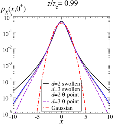
Figure 2: Unit-variance initial $x$-PDF for the CM of a linear polymer close to criticality. For comparison purposes, a unit-variance Gaussian PDF is also plotted in red dash-dotted line.

It is now interesting to discuss peculiar initial dynamical responses of polymers with different topologies, as $z\to z_{\mathrm{c}}$.
Linear polymers. In this case the condition $\gamma/2<\nu<\gamma$ is satisfied both in $d=2$ and $d=3$ (see first row in Fig 1) and the kurtosis diverges with exponents $5/32$ and $\simeq 0.012$, respectively – cf. Fig. 2.
$\mathcal{R}$-arms star polymers. In $d=2$ the kurtosis diverges if $\mathcal{R}\leq 4$, with exponent $2\nu-\gamma$ ($\mathcal{R}=2,3$) or $\gamma$ ($\mathcal{R}=4$). In $d=3$ the kurtosis diverges if $\mathcal{R}\leq 5$, with exponent $2\nu-\gamma$ ($\mathcal{R}=2,3,4$) or $\gamma$ ($\mathcal{R}=5$) – cf. Fig 3.
Rings and watermelon networks. Since $\gamma<0$ both in $d=2$ and $d=3$, $\kappa_{\mathrm{CM}}$ does not diverge.
Branched polymers (lattice animals). In $d=2$ $\gamma=0$ and the kurtosis diverges logarithmically, independently on the value of $\nu$. Instead, in $d=3$ $\gamma<0$, implying a finite value of $\kappa_{CM}$ also at the critical point.

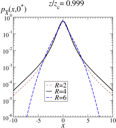
Figure 3: Unit-variance initial $x$-PDF for the CM of a star polymer in $d=3$ with different numbers of arms $\mathcal{R}$ close to criticality.

So far we have considered polymers whose equilibrium properties are dominated by monomer-solvent attraction (swollen phase). On the other hand, by varying solvent conditions polymers may undergo a thermodynamic transition from swollen (good solvent) to globular or compact phase (poor solvent). The transition occurs at a well defined critical phase known as $\Theta$-point, a genuine $O(n\to 0)$ tricritical point governing an equilibrium phase characterized by its own critical exponents $\gamma_{\Theta}$ and $\nu_{\Theta}$ de Gennes (1972); Vanderzande (1998). For instance, linear polymers at the $\Theta$-point in $d=2$ have $\nu_{\Theta}=4/7$ and $\gamma_{\Theta}=8/7$Duplantier and Saleur (1987); Duplantier (1988); Seno and Stella (1988); Vanderzande et al. (1991), whereas in $d=3$ the mean-field values $\nu_{\Theta}=1/2$ and $\gamma_{\Theta}=1$ are expected de Gennes (1979); Duplantier (1982). Hence, in both dimensions $\nu=\gamma/2$. This remarkable relation has the important consequence that as $z\to z_{c}$ the initial kurtosis diverges logarithmically for linear polymers at the $\Theta$-point, irrespective of the dimension. This result suggests that a change in the quality of the solvent driving dilute linear polymers close to $\Theta$-point, concomitantly mitigates the non-Gaussianity of the CM diffusion from power-law to logarithmic divergence of $\kappa_{CM}$. Fig. 2 displays the associated PDFs.

Finally, since the $\nu$ and $\gamma$ exponents depend on the embedding dimension $d$ of the system, transitions between phases with different effective dimension may also alter the non-Gaussianity of the initial CM diffusion. An example is the well studied de Gennes (1972); Vanderzande (1998) adsorption transition from the $d=3$ polymer swollen phase to the adsorbed ($d=2$) swollen phase. This is triggered by effective attractive interactions between monomers and an impenetrable surface. With a non negligible mobility of the polymer at the surface, the adsorption transition of linear polymers increases the exponent of the power law divergence of $\kappa_{CM}$ from $0.012$ ($d=3$) to $5/32$ ($d=2$).

We have analytically shown that the polymer critical state is the hallmark behind the non-Gaussian behavior of its CM. To each universality class, identified by the entropic and metric exponents $\gamma$ and $\nu$, corresponds a specific Brownian non-Gaussian diffusion of the polymer CM which crosses then over to ordinary Brownian motion above the polymerization autocorrelation time scale. This finding offers novel perspectives in stochastic modeling, as the anomalous stochastic process is not obtained here via a mesoscopic ansatz, but rather as a natural consequence of a microscopic foundation which can be worked out in all details and bridges the universal behavior of polymer systems at equilibrium with their short time anomalous dynamical response. The background we have evoked (different polymer architectures, $\Theta$- and adsorption transitions) is commonly operated in polymer experiments; this implies the exposed anomalous dynamics to be potentially triggered and highlighted in a variety of chemostatted experimental conditions.

References

- Wang et al. (2009) B. Wang, S. M. Anthony, S. C. Bae, and S. Granick, Proceedings of the National Academy of Sciences 106, 15160 (2009).
- Wang et al. (2012) B. Wang, J. Kuo, S. C. Bae, and S. Granick, Nature materials 11, 481 (2012).
- Toyota et al. (2011) T. Toyota, D. A. Head, C. F. Schmidt, and D. Mizuno, Soft Matter 7, 3234 (2011).
- Chakraborty and Roichman (2020) I. Chakraborty and Y. Roichman, Physical Review Research 2, 022020(R) (2020).
- Weeks et al. (2000) E. R. Weeks, J. C. Crocker, A. C. Levitt, A. Schofield, and D. A. Weitz, Science 287, 627 (2000).
- Wagner et al. (2017) C. E. Wagner, B. S. Turner, M. Rubinstein, G. H. McKinley, and K. Ribbeck, Biomacromolecules 18, 3654 (2017).
- Jeon et al. (2016) J.-H. Jeon, M. Javanainen, H. Martinez-Seara, R. Metzler, and I. Vattulainen, Physical Review X 6, 021006 (2016).
- Yamamoto et al. (2017) E. Yamamoto, T. Akimoto, A. C. Kalli, K. Yasuoka, and M. S. Sansom, Science advances 3, e1601871 (2017).
- Stylianidou et al. (2014) S. Stylianidou, N. J. Kuwada, and P. A. Wiggins, Biophysical journal 107, 2684 (2014).
- Parry et al. (2014) B. R. Parry, I. V. Surovtsev, M. T. Cabeen, C. S. O’Hern, E. R. Dufresne, and C. Jacobs-Wagner, Cell 156, 183 (2014).
- Munder et al. (2016) M. C. Munder, D. Midtvedt, T. Franzmann, E. Nuske, O. Otto, M. Herbig, E. Ulbricht, P. Müller, A. Taubenberger, S. Maharana, et al., elife 5, e09347 (2016).
- Cherstvy et al. (2018) A. G. Cherstvy, O. Nagel, C. Beta, and R. Metzler, Physical Chemistry Chemical Physics 20, 23034 (2018).
- Li et al. (2019) Y. Li, F. Marchesoni, D. Debnath, and P. K. Ghosh, Physical Review Research 1, 033003 (2019).
- Cuetos et al. (2018) A. Cuetos, N. Morillo, and A. Patti, Physical Review E 98, 042129 (2018).
- Hapca et al. (2008) S. Hapca, J. W. Crawford, and I. M. Young, Journal of the Royal Society Interface 6, 111 (2008).
- Pastore et al. (2021) R. Pastore, A. Ciarlo, G. Pesce, F. Greco, and A. Sasso, Physical Review Letters 126, 158003 (2021).
- Beck and Cohen (2003) C. Beck and E. G. Cohen, Physica A: Statistical mechanics and its applications 322, 267 (2003).
- Beck (2006) C. Beck, Progress of Theoretical Physics Supplement 162, 29 (2006).
- Chubynsky and Slater (2014) M. V. Chubynsky and G. W. Slater, Physical Review Letters 113, 098302 (2014).
- Chechkin et al. (2017) A. V. Chechkin, F. Seno, R. Metzler, and I. M. Sokolov, Physical Review X 7, 021002 (2017).
- Jain and Sebastian (2017) R. Jain and K. Sebastian, Journal of Chemical Sciences 129, 929 (2017).
- Tyagi and Cherayil (2017) N. Tyagi and B. J. Cherayil, The Journal of Physical Chemistry B 121, 7204 (2017).
- Miyaguchi (2017) T. Miyaguchi, Physical Review E 96, 042501 (2017).
- Sposini et al. (2018a) V. Sposini, A. V. Chechkin, F. Seno, G. Pagnini, and R. Metzler, New Journal of Physics 20, 043044 (2018a).
- Sposini et al. (2018b) V. Sposini, A. Chechkin, and R. Metzler, Journal of Physics A: Mathematical and Theoretical 52, 04LT01 (2018b).
- Miotto et al. (2021) J. M. Miotto, S. Pigolotti, A. V. Chechkin, and S. Roldán-Vargas, Physical Review X 11, 031002 (2021).
- Barkai and Burov (2020) E. Barkai and S. Burov, Physical Review Letters 124, 060603 (2020).
- Pacheco-Pozo and Sokolov (2021) A. Pacheco-Pozo and I. M. Sokolov, Physical Review Letters 127, 120601 (2021).
- Baldovin et al. (2019) F. Baldovin, E. Orlandini, and F. Seno, Frontiers in Physics 7, 124 (2019).
- Hidalgo-Soria and Barkai (2020) M. Hidalgo-Soria and E. Barkai, Physical Review E 102, 012109 (2020).
- Feller (1968) W. Feller, An Introduction to Probability Theory and Its Applications (John Wiley & Sons, 1968).
- de Gennes (1972) P.-G. de Gennes, Physics Letters A 38, 339–340 (1972).
- de Gennes (1979) P.-G. de Gennes, Scaling Concepts in Polymer Physics (Cornell University Press, 1979).
- Vanderzande (1998) C. Vanderzande, Lattice Models of Polymers (Cambridge University Press, 1998).
- Madras and Slade (2013) N. Madras and G. Slade, The Self-Avoiding Walk (Springer, 2013).
- Duplantier (1989) B. Duplantier, Journal of Statistical Physics 54, 581 (1989).
- Lubensky and Isaacson (1979) T. C. Lubensky and J. Isaacson, Physical Review A 20, 2130 (1979).
- Parisi and Sourlas (1981) G. Parisi and N. Sourlas, Physical Review Letters 46, 871 (1981).
- Brydges and Imbrie (2003) D. C. Brydges and J. Z. Imbrie, Annals of mathematics , 1019 (2003).
- Nienhuis (1982) B. Nienhuis, Physical Review Letters 49, 1062 (1982).
- Guida and Zinn-Justin (1998) R. Guida and J. Zinn-Justin, Journal of Physics A 31, 8103 (1998).
- Clisby (2010) N. Clisby, Physical Review Letters 104, 055702 (2010).
- Clisby (2017) N. Clisby, Journal of Physics A: Mathematical and Theoretical 50, 264003 (2017).
- Jensen (2001) I. Jensen, Journal of statistical physics 102, 865 (2001).
- not (a) This equation applies to the Smoluchowski time scale; the latter is appropriate for the description of the polyer dynamics at any sizes varying from single monomer to large colloids. Indeed, in the time needed to loose memory of inertial effects, the travelled distance with respect to the polymer radius is given by In water at room temperature, this ratio varies from for single nucleotides or amino acids to for large colloids (a).
- Doi and F (1992) M. Doi and E. S. F, The Theory of Polymer Dynamics (Oxford University Press, 1992).
- Yamamoto et al. (2021) E. Yamamoto, T. Akimoto, A. Mitsutake, and R. Metzler, Physical Review Letters 126, 128101 (2021).
- not (b) The value for the diffusion coefficient to be filled in Eq. (3) is the one coming from the hydrodynamic radius of the polymer Rubinstein and Colby (2003). Close to criticality, the latter is determined by the metric exponent as . So, Eq. (3) can be considered with both the exact values for the exponent and their approximations, like, e.g., the Flory one Doi and F (1992); Rubinstein and Colby (2003) (b).
- Bochner (2020) S. Bochner, Harmonic analysis and the theory of probability (University of California press, 2020).
- Odian (2004) G. Odian, Principles of Polymerization (John Wiley & Sons, 2004).
- Jain et al. (2007) J. L. Jain, S. G. Mohanty, and W. Böhm, A Course on Queueing Models (Chapman & Hall/CRC, 2007).
- Nampoothiri et al. (2021) S. Nampoothiri, E. Orlandini, F. Seno, and F. Baldovin, To be submitted (2021).
- Wang et al. (2020) W. Wang, F. Seno, I. M. Sokolov, A. V. Chechkin, and R. Metzler, New Journal of Physics 22, 083041 (2020).
- Duplantier and Saleur (1987) B. Duplantier and H. Saleur, Physical Review Letters 59, 539 (1987).
- Duplantier (1988) B. Duplantier, EPL (Europhysics Letters) 7, 677 (1988).
- Seno and Stella (1988) F. Seno and A. Stella, Journal de Physique 49, 739 (1988).
- Vanderzande et al. (1991) C. Vanderzande, A. L. Stella, and F. Seno, Physical Review Letters 67, 2757 (1991).
- Duplantier (1982) B. Duplantier, Journal de Physique 43, 991 (1982).
- Rubinstein and Colby (2003) M. Rubinstein and R. H. Colby, Polymer Physics (Oxford University Press, 2003).