Multiview point cloud registration with anisotropic and space-varying localization noise

Denis Fortun¹, Etienne Baudrier¹, Fabian Zwettler², Markus Sauer², Sylvain Faisan^{1 1} ICube - UMR7357, CNRS, University of Strasbourg ² Lehrstuhl für Biotechnologie und Biophysik, Biozentrum, Universität Würzburg, Germany

Abstract

In this paper, we address the problem of registering multiple point clouds corrupted with high anisotropic localization noise. Our approach follows the widely used framework of Gaussian mixture model (GMM) reconstruction with an expectation-maximization (EM) algorithm. Existing methods are based on an implicit assumption of space-invariant isotropic Gaussian noise. However, this assumption is violated in practice in applications such as single molecule localization microscopy (SMLM). To address this issue, we propose to introduce an explicit localization noise model that decouples shape modeling with the GMM from noise handling. We design a stochastic EM algorithm that considers noise-free data as a latent variable, with closed-form solutions at each EM step. The first advantage of our approach is to handle space-variant and anisotropic Gaussian noise with arbitrary covariances. The second advantage is to leverage the explicit noise model to impose prior knowledge about the noise that may be available from physical sensors. We show on various simulated data that our noise handling strategy improves significantly the robustness to high levels of anisotropic noise. We also demonstrate the performance of our method on real SMLM data.

1 Introduction

The acquisition of point cloud data has become ubiquitous for the perception of the 3D environment with the advent of sensors such as LiDAR and time-of-flight cameras, used for many applications in robotics, autonomous driving or augmented reality. The registration of point clouds is a fundamental step to achieve various tasks, including 3D scene reconstruction, pose estimation or localization. Besides these classical application fields, we particularly focus in this work on point cloud data acquired in single molecule localization microscopy (SMLM) [37], which is one of the reference techniques in fluorescence microscopy. Each point in SMLM represents the localization of a fluorophore attached to specific proteins, with a localization accuracy of a few nanometers. Registration plays an important role in SMLM in the single particle reconstruction paradigm [17], where multiple randomly oriented copies of a biological particle are registered in order to reconstruct a single 3D model with improved resolution.

Most registration methods are based on an iterative procedure that alternates between the computation of distances between points, and the estimation of a rigid transformation that aligns the point clouds. The iterative closest point (ICP) method is the oldest and most popular representative of this approach [3]. It retains only the smallest point-to-point distances to establish binary correspondences that enable a fast estimation of the optimal transformation parameters. However, the choice of binary correspondences limits the robustness of ICP to noise, missing data and initialization.

To circumvent this issue, the binary matches can be replaced by fuzzy correspondences. This generalization of ICP can be formalized by representing the target point cloud as a Gaussian mixture model (GMM) and solving a maximum likelihood clustering problem with an expectation-maximization algorithm (EM) [18, 8, 19]. This strategy can be generalized further by considering a generative approach [23, 11], where the GMM represents the distribution that generated both point clouds. In this framework, the GMM is estimated jointly with the rigid transformation. The generative approach can be naturally extended to the registration of multiple point sets, and it can reduce considerably the computational complexity when a low number of GMM components is used. A large proportion of multiview registration methods can be cast in this generative framework, which we will call EM-GMM in the remainder of the paper.

A major limitation of EM-GMM methods is the absence of explicit localization noise model. The localization noise comes from the measurement imperfection inherent to any physical acquisition devices. This is particularly true in SMLM where the points are estimated by a localization algorithm that usually provides known Gaussian uncertainty associated to each point, with a much higher variance in the axial direction of the microscope. To illustrate the amount of anisotropic noise in SMLM, we show in Figure 1 two acquisitions of a macromolecular assembly called centriole, which is known to have a barrel-like structure. The symmetry axis of the centriole is aligned with the axial direction z in the first acquisition (Fig. 1 a,c), and it is orthogonal to z in the second acquisition (Fig. 1 b,d). Fig 1.a and Fig. 1.b both show a view of the centriole in the direction of its symmetry axis, but the ring shape that corresponds to the circonference of the barrel is clearly retrieved in Fig 1.a, whereas the axial uncertainty completely blurs the shape in the z direction in Fig. 1.b. This example shows how the anisotropic noise can drastically modify the geometry of an object. Consequently, in the absence of noise model, two point clouds such as those of Fig. 1 cannot be represented by a common GMM, as it is done in the standard EM-GMM approach. The origin of the problem is that the GMM has to play two different roles: it has to fit both the shape of the object and the noise. Moreover, the absence of explicit noise model also prevents from incorporating prior knowledge about the localization uncertainty available in SMLM and potentially in other acquisition devices.

In this paper, we propose a generalization of EM-GMM registration methods that takes into account space-varying Gaussian localization noise with arbitrary covariances. We explicitly model the observed data as noisy measurement of unknown clean data. Thus, the GMM is fitted on the clean data to model the shape of the object, and it is decoupled from the noise model that generated the observed data. Since the clean data is unknown, our strategy is to consider it as a latent variable in the EM algorithm, which induces an additional marginalization in the expected log likelihood maximized in the EM algorithm. We use a stochastic EM approach to approximate the integral in the estimation of the rigid transformation parameters, and we derive analytical solutions at each step of the algorithm. We apply our strategy in the framework of the joint registration of multiple point clouds algorithm (JRMPC) [14], which is a generic EM-GMM method that can be applied to multiple point clouds. Our approach is generic and could also be integrated in the numerous EM-GMM variants of [14]. We show experimentally on simulated data that our method significantly improves registration and GMM reconstruction compared to the baseline method in the presence of high anisotropic and space varying noise. We also demonstrate the performance and interest of our approach on real SMLM data.

$\begin{array}[]{m{20pt}@{\hspace{0pt}}m{120pt}@{\hspace{0pt}}m{120pt}}\centering Top view\@add@centering&\centering\includegraphics[width=70.0pt]{figures/real_1_top_z_light}\@add@centering&\includegraphics[width=70.0pt]{figures/real_2_side_z_light}\\[-10.0pt] &\centering\mbox{(a)}\@add@centering&~{}~{}~{}~{}~{}~{}~{}~{}~{}~{}~{}\mbox{(b)}\\ \centering Side view\@add@centering&\centering\includegraphics[width=70.0pt]{figures/real_1_side_z_light}\@add@centering&\includegraphics[width=70.0pt]{figures/real_2_top_z_light}\\[-10.0pt] &\centering\mbox{(c)}\@add@centering&~{}~{}~{}~{}~{}~{}~{}~{}~{}~{}~{}\mbox{(d)}\end{array}$

Figure 1: Real data of centriole acquired with dStorm [20]. The two columns show two examples of point clouds, with a 90 degrees tilt of the centriole between the two views. The first row represent a view in the direction of the axis of symmetry of the centriole (top view), and the second row represents a view parallel to the axis of symmetry (side view).

2 Related works

In this section, we focus on reviewing the main EM-GMM strategies and their relation with noise handling.

The earliest works on the EM-GMM framework were dedicated to pairwise registration [8, 19]. The GMM was designed to fit the target point cloud by defining each of its points as the center of a Gaussian component. In this setting, the E-step amounts to the computation of weights of soft assignments, and the M-step is the estimation of the rigid transformation. The variances can be embedded in a coarse-to-fine scheme [19], or they can be estimated in the M-step [31, 23]. Several variants have been proposed to handle outliers [21], topological constraints [31], symmetrisation of the registration [9], or non rigid deformations [8]. This approach has been recently extended to the registration of multiple point clouds in [42], where a point is modeled as a mixture of Gaussians centered in the nearest neighbor points in each other point clouds.

From the point of view of noise modeling, this formulation is based on an assumption of Gaussian localization uncertainty of each point [19]. When the Gaussians have fixed isotropic covariances, the M-step has an analytical solution and it boils down to standard ICP with fuzzy correspondences. Some methods have extended this approach to handle anisotropic noise [13, 28]. The estimation of the transformation (M-step) becomes a generalized total least square problem that is solved with an iterative algorithm [32, 2]. Leveraging anisotropic covariances has also been proposed for the matching (E-step) in [28].

One of the main limitations of these methods is to rely on the assumption of perfect correspondences between noise-free points in the two point clouds. In practice, physical measurement devices are likely to produce different sampling schemes for each new acquisition. Consequently, the perfect correspondence assumption is violated in most cases. A proper noise modeling should decouple the localization uncertainty from the sampling uncertainty.

Moreover, this category of methods has two major limitations already mentioned in Section 1: it is restricted to pairwise registration (excluding [42]), and since there are as many Gaussian components as points, the computational complexity can become prohibitive. The generative EM-GMM methods [12, 14] have been developed to address these issues. They estimate the GMM as the common distribution of all the point clouds registered in the same pose. This is done by extending the M-step with the estimation of the means and covariances of the GMM in addition to the transformation parameters. It can be formalized as a conditional EM procedure [14].

In order to improve the robustness of the baseline approach [14], some works extended it to handle data composed of both point localization and orientation [4, 35, 30] with a Hybrid mixture model. Modeling outlier points and missing data is also a recurrent issue that is usually addressed with an additional uniformly distributed class [8, 31, 14], or replacing the GMM distribution with a Student’s t-mixture model [34].

The generative methods implicitly assume that the localization noise in the data is Gaussian and spatially invariant. The vast majority of methods consider isotropic covariance of the Gaussian components. An anisotropic variant can be found in [12], but the critical step of estimation of the transformation parameters in the M-step is performed with an isotropic approximation of the covariance, so the anisotropy is not properly handled throughout the algorithm. A solution for the M-step is proposed in [11] with a linear approximation valid only for small angles. Moreover, as mentioned in Section 1, prior knowledge about the noise covariance cannot be included in the model since it is implicitly contained in the covariances of the estimated Gaussian components.

Note that recent methods based on deep neural networks [1, 39, 41] also do not rely on explicit noise modeling. These methods are either based on the computation of local [39, 41] or global (PointNet) [1] features. However, the anisotropic noise in SMLM can drastically modify (locally ang globally) the geometry of an object (see Fig. 1). Consequently, we experimented that these registration algorithms fail to register SMLM data. In [15], we proposed a neural network approach dedicated to the special case of cylindrically symmetric shapes. It yields a coarse alignment and cannot be applied to non-symmetric structures.

Multiview registration in the context of SMLM data has been investigated in a few works. However, the problem is addressed in a simplified setting. In [6], a template is assumed to be available and is used as a target for pairwise registration. In [36], point clouds data is transformed to produce 2D image projections, which are used to apply standard reconstruction methods developed for tomography with unknown angles in cryo-electron microscopy. Finally, [22] uses the motion averaging framework, based on the computation of all pairwise registrations between input point clouds, followed by a global fusion of the transformation parameters. The pairwise registration step is performed with the method described in [25], which assumes isotropic noise, which is incompatible with the highly anisotropic localization uncertainty of SMLM data.

We also mention that the derivation of a GMM clustering method in the presence of uncertainty in the data has been introduced in [33] in the context of acoustic data. Our work is inspired from the solution of [33] for the GMM fitting part of our algorithm.

3 Registration with anisotropic uncertainty modelling

3.1 Generative formulation with noise modelling

We have $M$ point clouds denoted by $\overline{{\mathbf{y}}}_{j}=(\overline{{\mathbf{y}}}_{j1},\ldots,\overline{{\mathbf{y}}}_{jN_{j}})\in\mathbb{R}^{3\times N_{j}}$, where $N_{j}$ is the number of points of the $j$th point cloud. The total number of points is denoted $N=\sum_{j=1}^{M}N_{j}$. The goal is to estimate a rigid transformation composed of a rotation matrice ${\mathbf{R}}_{j}\in\mathbb{R}^{3\times 3}$ and a translation vector ${\mathbf{t}}_{j}\in\mathbb{R}^{3}$ for each point cloud such that the $M$ transformed points clouds ${\mathbf{R}}_{j}\overline{{\mathbf{y}}}_{j}+{\mathbf{t}}_{j}$ with $j=1,\ldots,M$ are in the same pose.

In the generative formulation of [14], the aligned points are assumed to be drawn from the same distribution, modeled as a GMM composed of $K$ Gaussian components. Thus, the GMM acts as a clustering of the union of all registered point clouds. Our purpose is to introduce to this model an explicit noise prior. To this end, we model the observed points clouds $\overline{\mathbf{y}}=\{\overline{\mathbf{y}}_{j}\}_{j=1,\ldots,M}$ as noisy versions of unknown clean point clouds ${\mathbf{y}}=\{{\mathbf{y}}_{j}\}_{j=1,\ldots,M}$. The distribution of each point $\overline{\mathbf{y}}_{ji}$ is an independent Gaussian pertubation from ${\mathbf{y}}_{ji}$

$$p(\overline{\mathbf{y}}_{ji}|{\mathbf{y}}_{ji})={\mathcal{N}}(\overline{\mathbf{y}}_{ji};{\mathbf{y}}_{ji},\overline{\boldsymbol{\Sigma}}_{ji}),$$ (1)

where $\overline{\boldsymbol{\Sigma}}_{ji}$ is the known covariance matrix of the measurement noise and

$${\mathcal{N}}({\mathbf{x}};\boldsymbol{\mu},\boldsymbol{\Sigma})=\frac{1}{\sqrt{(2\pi)^{3}|\boldsymbol{\Sigma}|}}\exp\left(-\frac{1}{2}\|{\mathbf{x}}-\boldsymbol{\mu}\|^{2}_{\boldsymbol{\Sigma}}\right),$$ (2)

with $\|{\mathbf{x}}-\boldsymbol{\mu}\|^{2}_{\boldsymbol{\Sigma}}=({\mathbf{x}}-\boldsymbol{\mu})^{T}\boldsymbol{\Sigma}^{-1}({\mathbf{x}}-\boldsymbol{\mu})$.

The distribution of the unknown clean data is represented by the GMM

$$p({\mathbf{y}}_{ji}|\theta)=\sum_{k=1}^{K}p_{k}{\mathcal{N}}(\phi_{j}({\mathbf{y}}_{ji});\boldsymbol{\mu}_{k},\boldsymbol{\Sigma}_{k}),$$ (3)

where $\boldsymbol{\mu}_{k}\in\mathbb{R}^{3}$, $\boldsymbol{\Sigma}_{k}\in\mathbb{R}^{3\times 3}$ and $p_{k}\in\mathbb{R}^{+}$ are the mean, covariance matrix and weight of the $k$th GMM component, respectively, $\phi_{j}({\mathbf{x}})={\mathbf{R}}_{j}{\mathbf{x}}+{\mathbf{t}}_{j}$ is the rigid transformation of the $j$th point cloud, and $\theta=\left\{\{\boldsymbol{\mu}_{k},\boldsymbol{\Sigma}_{k},p_{k}\}_{k=1}^{K},\{{\mathbf{R}}_{j},{\mathbf{t}}_{j}\}_{j=1}^{M}\right\}$ regroups the parameters of the rigid transformation and the GMM. Note that the probability $p({\mathbf{y}}_{ji}|\theta)$ is well defined as a function of $\phi_{j}({\mathbf{y}}_{ji})$ because $\phi_{j}$ is an invertible one-to-one mapping with a Jacobian determinant equal to one.

3.2 Maximum likelihood estimation with partially stochastic EM algorithm

3.2.1 Maximum likelihood estimation

Under the independence assumption of each point, the likelihood of the point clouds is defined as

$$L(\theta)=p(\overline{{\mathbf{y}}}|\theta)=\prod_{j=1}^{M}\prod_{i=1}^{N_{j}}p(\overline{{\mathbf{y}}}_{ji}|\theta).$$ (4)

To find the expression of $p(\overline{{\mathbf{y}}}_{ji}|\theta)$, we have to marginalize over the unknown clean data ${\mathbf{y}}_{ji}$:

$$p({\overline{\mathbf{y}}_{ji}}|\theta)=\int_{{\mathbf{y}}_{ji}}p(\overline{\mathbf{y}}_{ji}|{\mathbf{y}}_{ji})p({\mathbf{y}}_{ji}|\theta)d{\mathbf{y}}_{ji}.$$ (5)

We show in Appendix A that it can be written

$$p({\overline{\mathbf{y}}_{ji}}|\theta)=\sum_{k=1}^{K}p_{k}{\mathcal{N}}(\phi_{j}(\overline{\mathbf{y}}_{ji});\boldsymbol{\mu}_{k},\boldsymbol{\Sigma}_{k}+\overline{\boldsymbol{\Sigma}}_{ji}^{{\mathbf{R}}_{j}}),$$ (6)

where $\overline{\boldsymbol{\Sigma}}_{ji}^{{\mathbf{R}}_{j}}={\mathbf{R}}_{j}\overline{\boldsymbol{\Sigma}}_{ji}{\mathbf{R}}_{j}^{T}$ is the noise covariance rotated by ${\mathbf{R}}_{j}$. Thus, the likelihood function writes

$$L(\theta)=\prod_{j=1}^{M}\prod_{i=1}^{N_{j}}\sum_{k=1}^{K}p_{k}\,{\mathcal{N}}(\phi_{j}(\overline{\mathbf{y}}_{ji});\boldsymbol{\mu}_{k},\boldsymbol{\Sigma}_{k}+\overline{\boldsymbol{\Sigma}}_{ji}^{{\mathbf{R}}_{j}}).$$ (7)

In the standard case [14], the likelihood has the same general form, but the covariance of the Gaussian components are $\boldsymbol{\Sigma}_{k}$, instead of $\boldsymbol{\Sigma}_{k}+\overline{\boldsymbol{\Sigma}}_{ji}^{{\mathbf{R}}_{j}}$ in (7). Thus, the GMM covariance $\boldsymbol{\Sigma}_{k}$ implicitly contains the noise covariance. If $\boldsymbol{\Sigma}_{k}$ is isotropic (which is required to ensure a reasonable computational cost), this standard model is restricted to isotropic and shift invariant noise covariance. In our formulation (7), the noise covariance of each point $\overline{\boldsymbol{\Sigma}}_{ji}^{{\mathbf{R}}_{j}}$ is decoupled from the Gaussian clusters covariance $\boldsymbol{\Sigma}_{k}$. This opens the way to anisotropic and spatially varying noise, and it allows us to use prior knowledge of the noise covariance $\overline{\boldsymbol{\Sigma}}_{ji}$.

The optimization of the likelihood (7) is cumbersome and is achieved with the EM algorithm [10], which is a widely used procedure for estimating Gaussian mixture densities [5]. The EM algorithm introduces an auxiliary function $Q(\theta,\theta^{\prime})$, such that if $Q(\theta,\theta^{\prime})\geq Q(\theta^{\prime},\theta^{\prime})$, then $L(\theta)\geq L(\theta^{\prime})$. Based on this property, the EM algorithm proceeds by defining a series of models $\{{\theta}_{1},{\theta}_{2},\ldots\}$ such that ${\theta}^{(l+1)}$ maximizes $Q(\cdot,{\theta}^{(l)})$ and thereby $L({\theta}^{(l+1)})\geq L({\theta}^{(l)})$.

3.2.2 Derivation of the auxiliary function

To derive the auxiliary function, the problem is reformulated with the introduction of latent variables. In the conventional GMM case [5, 14], the latent variables ${\mathbf{z}}=\{z_{ji}\}_{j\in[1\ldots M],i\in[1\ldots N_{j}]}$ are defined such that the value of $z_{ji}\in[1,\ldots,K]$ indicates the Gaussian component assigned to the point ${\mathbf{y}}_{ji}$. The auxiliary function is then defined as the expected log-likelihood $E[\log(p(\overline{\mathbf{y}},{\mathbf{z}}|\theta))|\overline{\mathbf{y}},\theta^{(l)}]$, which involves a marginalization of over ${\mathbf{z}}$.

In this work, in addition to the Gaussian component assignment ${\mathbf{z}}$, we formalize the role of ${\mathbf{y}}$ by also considering it as latent data. Since there are two types of latent variables, the auxiliary function $Q(\theta,\theta^{(l)})$ is a marginalization over ${\mathbf{z}}$ and ${\mathbf{y}}$:

$$\begin{split}Q(\theta,\theta^{(l)})&=E[\log(p(\overline{\mathbf{y}},{\mathbf{y}},{\mathbf{z}}|\theta))|\overline{\mathbf{y}},\theta^{(l)}]\\ &=\sum_{\mathbf{z}}\int_{\mathbb{{\mathbf{y}}}}p({\mathbf{y}},{\mathbf{z}}|\overline{\mathbf{y}},\theta^{(l)})\log(p(\overline{\mathbf{y}},{\mathbf{y}},{\mathbf{z}}|\theta))d{\mathbf{y}},\end{split}$$ (8)

The term $p(\overline{\mathbf{y}},{\mathbf{y}},{\mathbf{z}}|\theta)$ of (8) is called the complete-data likelihood, as opposed to the incomplete-data likelihood (7). In our application, we have

$$\begin{split}p(\overline{\mathbf{y}},{\mathbf{y}},{\mathbf{z}}|\theta)&=\prod_{j=1}^{M}\prod_{i=1}^{N_{j}}p(\overline{\mathbf{y}}_{ji}|{\mathbf{y}}_{ji})p({\mathbf{y}}_{ji}|z_{ji},\theta)p(z_{ji}|\theta)\\ &=\prod_{j=1}^{M}\prod_{i=1}^{N_{j}}p_{z_{ji}}{\mathcal{N}}(\overline{\mathbf{y}}_{ji};{\mathbf{y}}_{ji},\overline{\boldsymbol{\Sigma}}_{ji})\,{\mathcal{N}}(\phi_{j}(\overline{\mathbf{y}}_{ji});\boldsymbol{\mu}_{z_{ji}},\boldsymbol{\Sigma}_{z_{ji}}+\overline{\boldsymbol{\Sigma}}_{ji}^{{\mathbf{R}}_{j}}).\end{split}$$ (9)

Using (9) and following the same strategy than for the standard GMM case [5], we show in Appendix B that (8) writes

$$\begin{split}Q(\theta,\theta^{(l)})=(constant)-\frac{1}{2}\sum_{jik}\Bigg{[}\alpha_{jik}\int_{{\mathbf{y}}_{ji}}\beta_{jik}({\mathbf{y}}_{ji})\left(\|\phi_{j}({\mathbf{y}}_{ji})-\boldsymbol{\mu}_{k}\|^{2}_{\boldsymbol{\Sigma}_{k}}+\log\left|\boldsymbol{\Sigma}_{k}\right|-2\log(p_{k})\right)d{\mathbf{y}}_{ji}\Bigg{]},\end{split}$$ (10)

where we use the notation $\sum_{jik}=\sum_{j=1}^{M}\sum_{i=1}^{N_{j}}\sum_{k=1}^{K}$, and where

$$\begin{gathered}\beta_{jik}({\mathbf{y}}_{ji})=p({\mathbf{y}}_{ji}|z_{ji}=k,\overline{\mathbf{y}}_{ji},\theta^{(l)}),\\ \alpha_{jik}=p(z_{ji}=k|\overline{\mathbf{y}}_{ji},\theta^{(l)})\end{gathered}$$ (11)

are the conditional distributions of the latent data. Note that the auxiliary function in [14] can be obtained by replacing in (10) the term $\beta_{jik}({\mathbf{y}}_{ji})$ by $\delta({\mathbf{y}}_{ji}-\overline{\mathbf{y}}_{ji})$, where $\delta$ is the Dirac function, which removes the integral over the clean data ${\mathbf{y}}$. The major difficulty in our case is to deal with this integral in the maximization of Q in (10).

To lighten the notations in what follows, the parameters of $\theta^{(l)}$ and $\theta$ will be both denoted $p_{k}$, $\boldsymbol{\mu}_{k}$, $\boldsymbol{\Sigma}_{k}$, ${\mathbf{R}}_{j}$ and ${\mathbf{t}}_{j}$, without reference to the iteration number $l$.

Using (6), the expression of $\alpha_{jik}$ is simply:

$$\alpha_{jik}=\frac{\gamma_{jik}}{\sum_{s=1}^{K}\gamma_{jis}},$$ (12)

where

$$\gamma_{jik}=p_{k}{\mathcal{N}}(\phi_{j}({\mathbf{y}}_{ji});\boldsymbol{\mu}_{k},\boldsymbol{\Sigma}_{k}+\overline{\boldsymbol{\Sigma}}_{ji}^{{\mathbf{R}}_{j}}).$$ (13)

We detail in Appendix C the derivation of the expression of $\beta_{jik}$:

$$\beta_{jik}({\mathbf{y}}_{ji})={\mathcal{N}}(\phi_{j}({\mathbf{y}}_{ji});\hat{{\mathbf{y}}}_{jik},({\mathbf{I}}-{\mathbf{W}}_{jik})\boldsymbol{\Sigma}_{k})$$ (14)

where

$${\mathbf{W}}_{jik}=\boldsymbol{\Sigma}_{k}\left(\boldsymbol{\Sigma}_{k}+\overline{\boldsymbol{\Sigma}}_{ji}^{{\mathbf{R}}_{j}}\right)^{-1}$$

$$\hat{\mathbf{y}}_{jik}={\mathbf{W}}_{jik}(\phi_{j}(\overline{\mathbf{y}}_{ji})-\boldsymbol{\mu}_{k})+\boldsymbol{\mu}_{k}.$$

Based on (14), the point $\hat{\mathbf{y}}_{jik}$ can be seen as a denoised version of $\phi_{j}({\overline{\mathbf{y}}_{ji}})$ under the hypothesis that the point ${\mathbf{y}}_{ji}$ is assigned to the Gaussian component $k$.

3.2.3 Space-alternating generalized EM

In a conventional EM algorithm, the E-step would consist in computing the conditional distributions $\alpha_{jik}$ and $\beta_{jik}$, and the M-step would be the actual maximization of $Q(\theta,\theta^{(l)})$ defined in (10). However, maximizing $Q$ with respect to all the parameters in $\theta$ is here an intractable task. This issue can be circumvented by searching for $\theta$ that only guarantees an increase $Q(\theta,\theta^{(l)})>Q(\theta^{(l)},\theta^{(l)})$. This approach is called Generalized Expectation Maximization (GEM) and ensures that the likelihood increases along the iterations. Several GEM strategies can be considered.

In [14], an Expectation Conditional Maximization (ECM) algorithm [29] is used. The parameters $\theta$ are splitted in two parts: the GMM parameters $\theta_{G}=\{\boldsymbol{\mu}_{k},\boldsymbol{\Sigma}_{k},p_{k}\}_{k=1}^{K}$, and the transformation parameters $\theta_{T}=\{{\mathbf{R}}_{j},{\mathbf{t}}_{j}\}_{j=1}^{M}$. Accordingly, the M-step is splitted in subproblems related to each variable:

$$\theta_{T}^{(l+1)} = \underset{\theta_{T}}{\text{argmax}}\,Q(\{\theta_{T},\theta_{G}^{(l)}\},\theta^{(l)}).$$ (15)

$$\theta_{G}^{(l+1)} = \underset{\theta_{G}}{\text{argmax}}\,Q(\{\theta_{T}^{(l+1)},\theta_{G}\},\theta^{(l)}).$$ (16)

In this work, we use instead a Space-alternating generalized expectation maximization (SAGE) [16] algorithm. The parameters are, as in ECM, sequentially updated, but the conditional distributions are also updated at each step. The SAGE algorithm can be written

$$\theta_{T}^{(l+1)} = \underset{\theta_{T}}{\text{argmax}}\,Q(\{\theta_{T},\theta_{G}^{(l)}\},\theta^{(l)}).$$ (17)

$$\theta_{G}^{(l+1)} = \underset{\theta_{G}}{\text{argmax}}\,Q(\{\theta_{T}^{(l+1)},\theta_{G}\},\{\theta_{T}^{(l+1)},\theta_{G}^{(l)}\}).$$ (18)

The interest of SAGE is to benefit from the updated value $\theta^{(l+1)}_{T}$ to derive new conditional distributions when computing $\theta_{G}^{(l+1)}$ in (18). The counterpart is that the SAGE algorithm requires two E-steps per iteration whereas the ECM algorithm requires only one E-step per iteration.

The next two Sections detail how we solve the two subproblems (17) and (18). Without loss of generality and in order not to overload the notations, all parameters related to the second operand of $Q$ will be denoted $\theta^{(l)}$.

3.3 Update of the transformation parameters

The maximization with respect to $\theta_{T}$ (17) is not tractable because of the integral over ${\mathbf{y}}_{ji}$ in (10). To tackle this problem, we resort to a stochastic version of the EM algorithm [7]. The principle is to approximate the integral in the auxiliary function by stochastic simulation. This is achieved here by drawing a unique sample $\hat{\mathbf{y}}^{s}_{jik}$ from $\beta_{jik}(\cdot)={\mathcal{N}}(\cdot|\hat{{\mathbf{y}}}_{jik},({\mathbf{I}}-{\mathbf{W}}_{jik})\boldsymbol{\Sigma}_{k})$ for each $i,j,k$. Since the distribution $\beta_{jik}$ is defined in the referential of the aligned point clouds, we have to bring the sample back in the original referential by applying the inverse transform. We obtain ${\mathbf{y}}^{s}_{jik}={\mathbf{R}}_{j}^{T}(\hat{\mathbf{y}}_{jik}^{s}-{\mathbf{t}}_{j})$ (where we recall that ${\mathbf{R}}_{j}$ and ${\mathbf{t}}_{j}$ are the parameters $\theta_{T}^{(l)}$ of the previous iteration $l$). The auxiliary function (10) is then approximated by:

$$\begin{split}Q(\theta,\theta^{(l)})\approx(constant)-\frac{1}{2}\sum_{jik}\Bigg{[}\alpha_{jik}\left(\|\phi_{j}({\mathbf{y}}^{s}_{jik})-\boldsymbol{\mu}_{k}\|^{2}_{\boldsymbol{\Sigma}_{k}}-2\log(p_{k})+\log\left|\boldsymbol{\Sigma}_{k}\right|\right)\Bigg{]}.\end{split}$$ (19)

Thus, the estimation of the rigid transforms amounts to solve

$$\{{{\mathbf{R}}}^{(l+1)}_{j},{\mathbf{t}}^{(l+1)}_{j}\}=\underset{{\mathbf{R}}_{j},{\mathbf{t}}_{j}}{\text{argmin}}\,\sum_{jik}\alpha_{jik}\|\phi_{j}({\mathbf{y}}_{jik}^{s})-\boldsymbol{\mu}_{k}\|^{2}_{\boldsymbol{\Sigma}_{k}}.$$ (20)

Under the hypothesis $\boldsymbol{\Sigma}_{k}=\sigma_{k}^{2}{\mathbf{I}}$, this is a classical weighted Procruste problem that admits a closed form solution based on SVD [38, 14]. In the general case, the problem (20) can be solved using convex optimization tools [23].

Note that the auxiliary function could be approximated by a larger number of samples, which would lead to the Monte-Carlo EM approach [40], but we found experimentally that one sample was sufficient. We emphasize that our approach is partially stochastic since the simulation of samples is only applied to ${\mathbf{y}}_{ji}$, while the other latent variables $z_{ji}$ are handled as in deterministic EM. Algorithm 1 summarizes the different steps to update the transformation parameters.

Algorithm 1 Update of the transformation parameters

1:E-step: computation of conditional expectations and generation of samples according to $\beta_{jik}$.

2:$\gamma_{jik}=p_{k}{\mathcal{N}}(\phi_{j}({\mathbf{y}}_{ji})|\boldsymbol{\mu}_{k},\boldsymbol{\Sigma}_{k}+\overline{\boldsymbol{\Sigma}}_{ji}^{{\mathbf{R}}_{j}})$, $\alpha_{jik}=\frac{\gamma_{jik}}{\sum_{s=1}^{K}\gamma_{jis}}$

3:${\mathbf{W}}_{jik}=\boldsymbol{\Sigma}_{k}\left(\boldsymbol{\Sigma}_{k}+\overline{\boldsymbol{\Sigma}}_{ji}^{{\mathbf{R}}_{j}}\right)^{-1}$

4:$\hat{\mathbf{y}}_{jik}={\mathbf{W}}_{jik}(\phi_{j}(\overline{\mathbf{y}}_{ji})-\boldsymbol{\mu}_{k})+\boldsymbol{\mu}_{k}$

5:generate $\hat{\mathbf{y}}^{s}_{jik}$ by sampling from ${\mathcal{N}}(.|\hat{{\mathbf{y}}}_{jik},({\mathbf{I}}-{\mathbf{W}}_{jik})\boldsymbol{\Sigma}_{k})$

6:${\mathbf{y}}^{s}_{jik}={\mathbf{R}}_{j}^{T}(\hat{\mathbf{y}}_{jik}^{s}-{\mathbf{t}}_{j})$

7: M-rigid step: update the rigid transformation parameters

8:$\{{\mathbf{R}}^{(l+1)}_{j},{\mathbf{t}}^{(l+1)}_{j}\}=\underset{{\mathbf{R}}_{j},{\mathbf{t}}_{j}}{\text{argmin}}\,\sum_{jik}\alpha_{jik}\|\phi_{j}({\mathbf{y}}_{jik}^{s})-\boldsymbol{\mu}_{k}\|^{2}_{\boldsymbol{\Sigma}_{k}}$

3.4 Update of the parameters of the GMM

When the transformation parameters are fixed, the optimization problem (18) amounts to a GMM fitting on the union of the aligned point clouds $\{\phi_{j}(\overline{\mathbf{y}}_{ji})\}_{j=1\ldots M}$. In the noise-free case, the update equations are the same as in the standard GMM case [5, 14]. In our model, we have to deal with the integral over the clean data in (10), which makes the problem more difficult. We show in Appendix D that the following update equations can be derived from the expression of $Q$ in (10):

$$p^{(l+1)}_{k}=\frac{1}{N}\sum_{j=1}^{M}\sum_{i=1}^{N_{j}}\alpha_{jik},$$ (21)

$$\boldsymbol{\mu}_{k}^{(l+1)}=\frac{\sum_{j=1}^{M}\sum_{i=1}^{N_{j}}\alpha_{jik}E[\phi_{j}({\mathbf{y}}_{ji})]}{\sum_{j=1}^{M}\sum_{i=1}^{N_{j}}\alpha_{jik}},$$ (22)

$$\boldsymbol{\Sigma}_{k}^{(l+1)}=\frac{\sum_{j=1}^{M}\sum_{i=1}^{N_{j}}\alpha_{jik}E[(\phi_{j}({\mathbf{y}}_{ji})-\boldsymbol{\mu}_{k})(\phi_{j}({\mathbf{y}}_{ji})-\boldsymbol{\mu}_{k})^{T}]}{\sum_{j=1}^{M}\sum_{i=1}^{N_{j}}\alpha_{jik}},$$ (23)

with the notation $E[X]=\int_{y}\beta_{jik}(y)Xdy$. These updates have the same form as in the standard noise-free case. The only difference is that the terms that involve the unknown clean data $\phi_{j}({\mathbf{y}}_{ji})$ are replaced here by their conditional expectation. We show in Appendix D that these conditional expectations have simple closed forms. This leads to the update steps summarized in Algorithm 2.

Algorithm 2 Update of the parameters of the GMM

1:E-step: computation of conditional expectations

2:$\gamma_{jik}=p_{k}{\mathcal{N}}(\phi_{j}({\mathbf{y}}_{ji})|\boldsymbol{\mu}_{k},\boldsymbol{\Sigma}_{k}+\overline{\boldsymbol{\Sigma}}_{ji}^{{\mathbf{R}}_{j}})$, $\alpha_{jik}=\frac{\gamma_{jik}}{\sum_{s=1}^{K}\gamma_{jis}}$

3:${\mathbf{W}}_{jik}=\boldsymbol{\Sigma}_{k}\left(\boldsymbol{\Sigma}_{k}+\overline{\boldsymbol{\Sigma}}_{ji}^{{\mathbf{R}}_{j}}\right)^{-1}$

4:$\hat{\mathbf{y}}_{jik}={\mathbf{W}}_{jik}(\phi_{j}(\overline{\mathbf{y}}_{ji})-\boldsymbol{\mu}_{k})+\boldsymbol{\mu}_{k}$.

5:$\hat{{\mathbf{R}}}_{jik}=\hat{{\mathbf{y}}}_{ji}\hat{{\mathbf{y}}}_{ji}^{T}+({\mathbf{I}}-{\mathbf{W}}_{jik})\boldsymbol{\Sigma}_{k}$

6:M-GMM step: update the GMM parameters

7:$p_{k}^{(l+1)}=\frac{1}{N}\sum_{j=1}^{M}\sum_{i=1}^{N_{j}}\alpha_{jik}$

8:$\boldsymbol{\mu}_{k}^{(l+1)}=\frac{\sum_{j=1}^{M}\sum_{i=1}^{N_{j}}\alpha_{jik}\hat{\mathbf{y}}_{jik}}{\sum_{j=1}^{M}\sum_{i=1}^{N_{j}}\alpha_{jik}}$

9:$\boldsymbol{\Sigma}_{k}^{(l+1)}=\frac{\sum_{j=1}^{M}\sum_{i=1}^{N_{j}}\alpha_{jik}\hat{{\mathbf{R}}}_{jik}}{\sum_{j=1}^{M}\sum_{i=1}^{N_{j}}\alpha_{jik}}$

The same algorithm has previously been derived in [33] for GMM fitting with uncertainties on acoustic data. In [33], the update equations are directly given after showing that the complete data belongs to the exponential family. We follow here an alternative derivation from the auxiliary function $Q$, which provides details that are omitted in [33].

4 Implementation details

In practice, we do not use the update equation of the priors $p_{k}$ (21), in accordance with [14]. We observed that keeping them constant does not alter the convergence and the quality of the registration.

The methods described in Section 3 are not robust to outlier points that may not fit with the reconstructed GMM distribution. To overcome this issue, we use the standard approach that consists in adding a class dedicated to outliers, modeled by a uniform distribution. We did not include this outlier handling in the description of the method for the sake of clarity. When the outlier class is included, Eq. (3) becomes

$$p({\mathbf{y}}_{ji}|\theta)=\sum_{k=1}^{K}p_{k}{\mathcal{N}}(\phi_{j}({\mathbf{y}}_{ji});\boldsymbol{\mu}_{k},\boldsymbol{\Sigma}_{k})+p_{k+1}\mathcal{U}(h),$$ (24)

where $\mathcal{U}(h)$ is the uniform distribution parameterized by the volume of the 3D convex hull encompassing the data. Since the priors $\{p_{k}\}_{k=1\ldots K+1}$ are not updated, we can show that this modification only modifies the normalization in the computation of the posteriors $\alpha_{jik}$ in the E-step, such that (12) becomes (for $k=1\ldots K$):

$$\alpha_{jik}=\frac{\gamma_{jik}}{\sum_{s=1}^{K}\gamma_{jis}+\frac{p_{k+1}}{h}},$$ (25)

The outlier handling role of the normalization in (25) can be understood intuitively. Suppose that $\overline{\mathbf{y}}_{ji}$ is an outlier. Without this additional class, since we ensure $\sum_{k=1}^{K}\alpha_{jik}=1$, all points have a similar influence in the update of the parameters. However, with this additional class, as $\overline{\mathbf{y}}_{ji}$ is an outlier, we expect $\gamma_{jik}$ to be much smaller than $\frac{p_{k+1}}{h}$, so that the posterior $\alpha_{jik}$ is close to $0$ for $k=1...K$ ($\alpha_{jiK+1}$ is close to 1 since $\sum_{k=1}^{K+1}\alpha_{jik}=1$). This means that this point will have very few impacts on the update of the parameters.

As in [14], we consider GMM with isotropic covariances, i.e. $\boldsymbol{\Sigma}_{k}=\sigma^{2}_{k}I$. In this case, the update of the transformation parameters in (20) has a simple closed form solution. Concerning the update of the covariance of the GMM in Alg. 2, we can easily show that the variance parameter can be obtained by ${\sigma^{2}_{k}}^{(l+1)}=\text{trace}(\boldsymbol{\Sigma}_{k}^{(l+1)})/3$.

5 Experimental Results

In this section we provide an experimental analysis of our method on synthetic and real data. Since our algorithm is an extension of the baseline method JRMPC [14], we focus our evaluation on the comparison with this method.

5.1 Results on synthetic data

5.1.1 Dataset

$\begin{array}[]{c@{\hspace{0pt}}c}\includegraphics[width=100.0pt]{figures/centriole_view1_light}&\includegraphics[width=120.0pt]{figures/centriole_view2_light}\\ \includegraphics[width=120.0pt]{figures/triplets_view1.pdf}&\includegraphics[width=120.0pt]{figures/triplets_view2.pdf}\end{array}$

Figure 2: Simulated data of the centriole (top) and triplets (bottom).

$\begin{array}[]{c@{\hspace{0pt}}c@{\hspace{0pt}}c@{\hspace{0pt}}c}\mbox{Ground truth}&\mbox{$r=1$}&\mbox{$r=5$}&\mbox{$r=10$}\\ \includegraphics[width=115.0pt]{figures/bunny_gt_light}&\includegraphics[width=115.0pt]{figures/bunny_z1_light}&\includegraphics[width=115.0pt]{figures/bunny_z5_light}&\includegraphics[width=115.0pt]{figures/bunny_z10_light}\\ \includegraphics[width=115.0pt]{figures/centriole_gt_0-0_light}&\includegraphics[width=115.0pt]{figures/centriole_z1_0-0_light}&\includegraphics[width=115.0pt]{figures/centriole_z5_0-0_light}&\includegraphics[width=115.0pt]{figures/centriole_z10_0-0_light}\\ \end{array}$

Figure 3: Examples of simulated point clouds with different levels of anisotropic noise from the bunny (top) and centriole (bottom) models ($\sigma=0.01$ in all the examples).

Since our primary goal is to apply our algorithm to microscopy data, we simulated the tubulin structure of the centriole, which is a fundamental macromolecular assembly involved in most cellular processes. To this end, we used the structural analysis of [27], where detailed information about the geometry of the centriole is provided. Our simulated structure is shown in Figure 2. It is composed of 9 triplets of overlapping tubes, organized in a ninefold cylindrical symmetry (C9) around the z-axis. It creates a barrel-like structure, with a smaller radius at the top of the structure than at the bottom. We will call this object centriole. We also simulated an object composed of 54 source points also organized in triplets with a C9 symmetry (Figure 2). It is reminiscent of the structure of the centriole and of other biological particles such as nuclear pore. We will call this objet triplets. Finally, we also used the bunny model from the traditional Stanford dataset. We fix the number of points of the ground truth model to 2000 for centriole and bunny.

A point cloud is created by first rotating the ground truth model, then adding outliers drawn from a uniform law, and finally drawing points from the Gaussian uncertainty distribution $\overline{\boldsymbol{\Sigma}}_{ji}$. We consider uncertainties of the form

$$\overline{\boldsymbol{\Sigma}}_{ji}=\left(\begin{array}[]{ccc}\sigma&0&0\\ 0&\sigma&0\\ 0&0&r\sigma\\ \end{array}\right),$$ (26)

where $\sigma>0$ is the noise level and $r\geq 1$ imposes anisotropy in one direction. It mimics SMLM data, where the uncertainty in the axial direction is larger than in the lateral plane. To simulate space varying noise, the noise level at each point is defined as a sample of a Gaussian distribution centered on $\sigma$. In Figure 3, we show examples of simulated point clouds with several values of $r$. We fix the proportion of outliers points to $10\%$ in all our experiments. Finally, the number of point clouds has been set to $M=5$.

5.1.2 Error metric

Since the pose of the object of interest is arbitrary in the common space, we do not expect the estimated transformation $\hat{\phi}_{j}$ to be close to the inverse of the ground truth transformation $\widetilde{\phi}_{j}$, but we expect ${\hat{\phi}_{i}}\circ{\widetilde{\phi}_{i}}$ to be close to ${\hat{\phi}_{j}}\circ{\widetilde{\phi}_{j}}$, for $(i,j)\in[1,M]^{2}$. The translation parameters are easy to estimate (when the rotation parameters are well-estimated), so we only consider the rotation parameters to evaluate the accuracy of the registration. Thus, our error metric is defined as the distance between the matrices ${\hat{R}_{i}}{\widetilde{R}_{i}}$ and ${\hat{R}_{j}}{\widetilde{R}_{j}}$, or equivalently between the matrices ${\hat{R}_{ij}}={\hat{R}_{i}}^{T}{\hat{R}_{j}}$ and ${\widetilde{R}_{ij}}={\widetilde{R}_{i}}{\widetilde{R}_{j}}^{T}$. Several functions have been proposed to measure the distance between 3D rotation matrices [24]. The distance $d_{ij}$ between $\hat{R}_{ij}$ and $\widetilde{R}_{ij}$ can be computed from the angle of the rotation matrix ${\hat{R}_{ij}}{\widetilde{R}_{ij}}^{T}$ (that should be close to the identity matrix). This angle can be computed using the quaternion representation (as in [24]), or simply by:

$$\theta_{ij}=\arccos\left(\frac{\text{tr}({\hat{R}_{ij}}{\widetilde{R}_{ij}}^{T})-1}{2}\right).$$ (27)

The distance $d_{ij}$ is then

$$d_{ij}=\min(\theta_{ij},\pi-\theta_{ij})$$ (28)

(it is possible to compute $d_{ij}$ directly from (27) by using an absolute value for the term inside the $acos$ function).

The centriole and triplets models have a ninefold cylindrical symmetry with respect to the z-axis. This means that the rotation by an angle of $2k\pi/9$ ($k=0\ldots 8$) does not change the object. In this case, the error metric has to be adapted since there are nine correct rotation parameters. We write $d_{ij}(k)$ the distance defined in (28) between ${\hat{R}_{ij}}={\hat{R}_{i}}^{T}{\hat{R}_{j}}$ and ${\widetilde{R}_{ij}}(k)={\widetilde{R}_{i}}R_{z}(k)^{T}{\widetilde{R}_{j}}^{T}$, where $R_{z}(k)$ defines the rotation matrix around the z-axis by an angle of $2k\pi/9$. We define the error metric by computing the nine possible cases and selecting the minimum value: $d_{ij}=\min_{k=0\ldots 8}d_{ij}(k)$.

$\begin{array}[]{c@{\hspace{0pt}}c@{\hspace{0pt}}c}\mbox{\it{Triplets}}&\mbox{\it{Centriole}}&\mbox{\it{Bunny}}\\[-1.0pt] \includegraphics[width=160.0pt]{figures/influence_z_triplets_K54.pdf}&\includegraphics[width=160.0pt]{figures/influence_z_centriole_K500.pdf}&\includegraphics[width=160.0pt]{figures/influence_z_bunny_K1000.pdf}\\ \includegraphics[width=160.0pt]{figures/influence_u_triplets_K54.pdf}&\includegraphics[width=160.0pt]{figures/influence_u_centriole_K500.pdf}&\includegraphics[width=160.0pt]{figures/influence_u_bunny_K1000.pdf}\\ \end{array}$

Figure 4: Impact of different noise parameters on the registration error. Top row: influence of $r$ with $\sigma=0.01$; Bottom row: influence of $\sigma$ with $r=5$. The vertical bar represents the standard deviation of the error.

	$\sigma=0.01$, $r=10$		$\sigma=0.05$, $r=5$
Our method
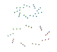
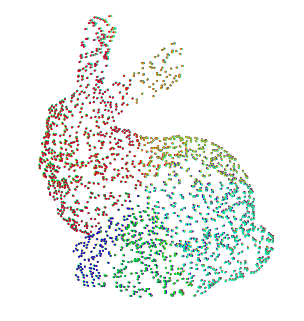
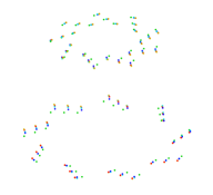
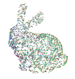
	error = 1.63	error = 0.81	error = 2.92	error = 3.03
JRMPC
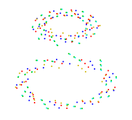
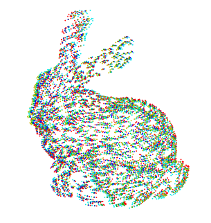
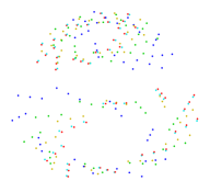
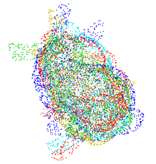
	error = 12.9	error = 4.3	error = 20.1	error = 50.2

Figure 5: Visual results of the registration of 5 point clouds generated from the triplets and bunny models, for different levels of noise. We show the ground truth models that were used to generate the point clouds (each point cloud has a different color), registered with our method (top row) and JRMPC (bottom row). We consider two combinations of noise parameters: $(\sigma=0.01$, $r=10)$ on the first two columns and $(\sigma=0.05$, $r=5)$ on the last two columns. The quantitative error is given for each case.

$\begin{array}[]{m{80pt}@{\hspace{0pt}}m{80pt}@{\hspace{0pt}}m{80pt}@{\hspace{0pt}}m{80pt}@{\hspace{0pt}}m{80pt}@{\hspace{0pt}}m{80pt}}\centering\mbox{Ground truth}\@add@centering&\centering\mbox{Our method}\@add@centering&\centering\mbox{JRMPC}\@add@centering&\centering\mbox{Ground truth}\@add@centering&\centering\mbox{Our method}\@add@centering&~{}~{}~{}~{}~{}\mbox{JRMPC}\\ \includegraphics[width=75.0pt]{figures/gt_triplets_side_crop&\includegraphics[width=75.0pt]{figures/recon_triplets_ours_side_crop&\includegraphics[width=75.0pt]{figures/recon_triplets_jrmpc_side_crop&\includegraphics[width=75.0pt]{figures/gt_triplets_top_crop&\includegraphics[width=75.0pt]{figures/recon_triplets_ours_top_crop&\includegraphics[width=75.0pt]{figures/recon_triplets_jrmpc_top_crop}\\ \includegraphics[width=75.0pt]{figures/gt_centriole_side_crop_light&\includegraphics[width=75.0pt]{figures/recon_centriole_ours_side_crop&\includegraphics[width=75.0pt]{figures/recon_centriole_jrmpc_side_crop&\includegraphics[width=75.0pt]{figures/gt_centriole_top_crop_light&\includegraphics[width=75.0pt]{figures/recon_centriole_ours_top_crop&\includegraphics[width=75.0pt]{figures/recon_centriole_jrmpc_top_crop}\\ \includegraphics[width=70.0pt]{figures/gt_bunny_side_crop_light&\includegraphics[width=75.0pt]{figures/recon_bunny_ours_side_crop&\includegraphics[width=75.0pt]{figures/recon_bunny_jrmpc_side_crop&\includegraphics[width=70.0pt]{figures/gt_bunny_top_crop_light&\includegraphics[width=75.0pt]{figures/recon_bunny_ours_top_crop&\includegraphics[width=75.0pt]{figures/recon_bunny_jrmpc_top_crop}\\ \end{array}}}}}}}}}}}}}}}}$

Figure 6: Comparison of the centers of the estimated GMM obtained with our method and JRMPC for the triplets (top row), centriole (middle row), and Bunny (bottom row). Two different views are shown in each case: the first view is on the first three columns and the second view is on the last three columns. The noise parameters have been set to $\sigma=0.01$ and $r=5$.

5.1.3 Hyperparameter setting and initialization

We observed that the number of Gaussian components $K$ does not have a substantial impact on the registration results as long as $K$ is of the same order of magnitude as the number of points. We fixed $K=54$ for the triplets, $K=1500$ for the centriole and $K=2500$ for the bunny.

As explained in the previous section and as in [13], the priors $p_{k}$ are not updated and are all set to the same value except $p_{K+1}$ that represents the outlier probability. The proportion of outliers can be defined as

$$\gamma=\frac{p_{K+1}}{\sum_{k=1}^{K}p_{k}}=\frac{p_{K+1}}{Kp_{1}}.$$ (29)

We observed that variations of the value of $\gamma$ had very little impact on the registration results. In the following, the priors $p_{k}$ have been set so that $\gamma=0.1$.

Initialization plays a crucial role in EM procedures. As in [14], we suppose we have a rough initialization of the transformation parameters. Rotation parameters are initialized by drawing the Euler angles from a Gaussian law centered on the ground truth angles, with a standard deviation of $30$ degrees. For the initialization of the GMM, we use these transformation parameters to transform each point set to the common space and we select randomly $K$ different points among the $M$ transformed points to initialize $\mu_{k}$. The variances $\sigma_{k}$ are initialized with high values.

We use the same hyperparameters and initialization for JRMPC and our method. To account for the random nature of the initialization, we run both algorithms five times with different GMM initializations and retain for each one the result with the highest likelihood.

5.1.4 Analysis of the results

We are particularly interested in the robustness to noise, which is determined by the noise level $\sigma$ and the anisotropy parameter $r$ defined in (26). In Figure 4, we show the influence of $\sigma$ and $r$ on the registration error for our method and JRMPC. As expected, we first observe that the two methods provide comparable results when the anisotropy parameter $r$ is equal to 1. Indeed, the implicit assumption of JRMPC is isotropic Gaussian noise. The differences for $r=1$ can be explained by the fact that we apply Gaussian noise with spatially varying covariance, which violates the model of JRMPC. We also observe that when the anisotropy parameter $r$ grows (with a fixed noise level $\sigma$), the error increases much slower with our method than with JRMPC (top line of Fig. 4). This highlights the benefit of the proposed modeling. Finally, the same behavior occurs when the noise level $\sigma$ increases with a fixed $r$ (bottom line of Fig. 4). For low noise levels, the original data is only slightly corrupted by noise and the influence of the anisotropy parameter is negligible, whereas for higher noise levels the influence of the anisotropy parameter becomes preponderant, which explains the better performances of our method.

In Figure 5, we illustrate the visual quality of the registration results associated to the quantitative errors of Fig. 4. Since the input point clouds are corrupted with a high level of noise, their mere superimposition after registration is not informative enough about the quality of the registration. Therefore, we show instead the underlying ground truth models that were used to generate the data. We consider two combinations of noise parameters (($\sigma=0.01$, $r=10$) and ($\sigma=0.05$, $r=5$)), and we give the associated quantitative error. In the case ($\sigma=0.01$, $r=10$), the registration with our method is almost perfect, while the results of JRMPC are less accurate. In the higher noise regime ($\sigma=0.05$, $r=5$), our results stay visually satisfying, but JRMPC completely fails to estimate correct registration parameters.

It is also interesting to look at the GMM density estimated jointly with the registration parameters. We show in Figure 6 the centers of the Gaussian components of the GMM estimated with our method and JRMPC, for a medium noise level defined by $\sigma=0.01$ and $r=5$. We can see in each case that the GMM estimated with our method recovers sharper details of the original shapes.

These results show how the integration of our noise model in the EM estimation improves both numerically and visually the registration results. This is explained by the fact that with JRMPC, each Gaussian component of the GMM has to account both for the shape of the object and the noise. Therefore, the reconstructed GMM of Figure 6 tends to fit the noise with JRMPC. Our method decouples noise handling from shape modeling, such that the GMM actually fits only the shape of the objects in Figure 6. Since the GMM acts as a target for the registration of the input point clouds in the EM algorithm, the quality of the registration is directly intertwined with the quality of the GMM reconstruction.

5.2 Real data

We applied our method on real microscopy data. We used direct stochastic optical reconstruction microscopy (dStorm), which one of the most popular SMLM techniques, combined with expansion microscopy [43]. It produces point clouds with a known anisotropic localization uncertainty of the form (26). We imaged the tubulin structure of the centriole, which is a macromolecular assembly that plays a crucial role in several cellular mechanisms and has motivated a lot of recent research to decipher its structural properties [26]. It is know to have a barrel-like shape and a C9 symmetry structure, from which our centriole simulated structure is inspired from (see Fig. 3). The acquired point cloud contained several centrioles, and we manually cropped ten of them, shown in Fig. 1.e-f, to perform registration. As already discussed in Section 1 and Figure 1, we can see that the noise in the axial direction z of the microscope is much higher than in the lateral plane. The localization noise of each point is known and follows a Gaussian law with a covariance of the form (26). The experimental distribution of the anisotropy parameter $r$ can be approximated by a Gaussian law with mean 5 and standard deviation 1.5. Therefore, it is crucial to combine the information of each view to reconstruct high resolution particles. Fig 7 shows all the input point clouds in their original pose. We initialize the registration parameters with the coarse registration method dedicated to centrioles described in [15].

The reconstruction of the GMM is of particular interest in our application since our goal is to reconstruct a model of the particle with a higher resolution than in the original data. The estimated centers of the GMM can serve as such a reconstruction. In Fig. 8, we show the centers estimated with our method and JRMPC. Similarly to the simulated case, we observe that our method captures more precisely the shape of the centriole, and the reconstruction of JRMPC is more influenced by the presence of noise. To obtain Fig. 8.c and 8.f, we created volumes by summing Gaussians of fixed variance centered on each of the estimated centers, and we projected the volumes in the direction of the symmetry axis of the centriole. With our method we can recover the ninefold symmetry of the centriole in Fig. 8.c, whereas the JRMPC result is much more blurred. This shows that our noise handling approach can reveal biologically relevant information that is lost with the baseline method.

In Fig. 9.a,b,e,f we show the registered point clouds obtained with the two methods. It is difficult to visually assess the quality of the registration because of the high amount of noise. Therefore, we show in In Fig. 9.c,d,g,h cleaned versions of the registered point clouds. They are obtained by applying the postprocessing described in [14] that removes points classified as outliers and points assigned to Gaussian components with high variance (superior to 2.5 times the median variance). A Gaussian component with high variance means that it does not cluster accurately the shape of the object and is likely to also capture noise. We see that the cleaned point clouds remain very noisy with JRMPC, while our clean data recovers the shape of the centriole. This means that the variances of the GMM clusters do not capture noise and are concentrated on the particle.

$\begin{array}[]{m{120pt}@{\hspace{0pt}}m{120pt}}\includegraphics[width=120.0pt]{figures/real_superp_top_z_light&\includegraphics[width=120.0pt]{figures/real_superp_side_z_light}\end{array}}$

Figure 7: Superimposition of the ten real dStorm acquisitions of centriole in their original pose (the red and blue point clouds are presented individually in Figure 1). The first column represents a view orthogonal to the $z$ direction, and the second column represents a view parallel to the $z$ direction.

Our method
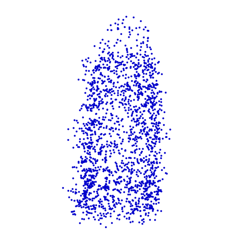
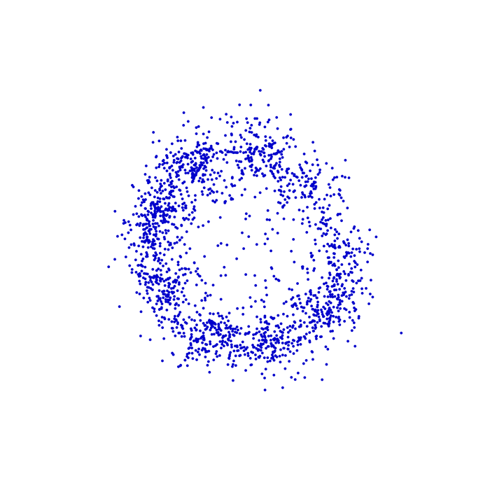
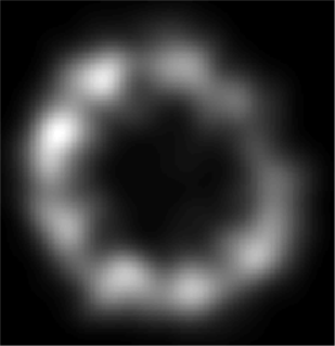
	(a)	(b)	(c)
JRMPC
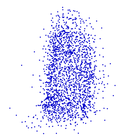
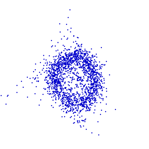
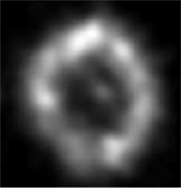
	(d)	(e)	(f)

Figure 8: Centers of the estimated GMM on real data. The first two columns are two orthogonal views. The last column shows the projection in the direction of the centriole axis of the volume obtained by evaluating the GMM on a 3D grid.

	Original data		Cleaned data
Our method
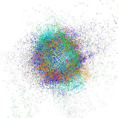
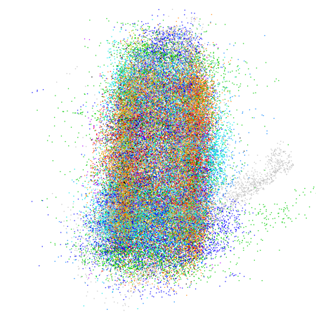
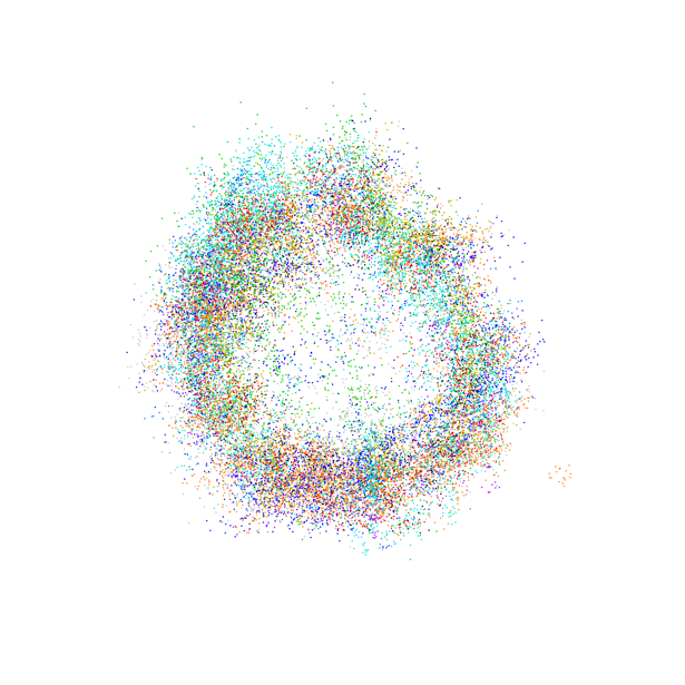
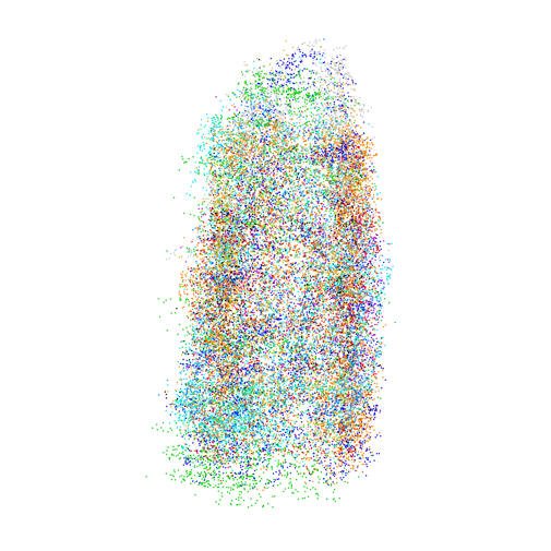
	(a)	(b)	(c)	(d)
JRMPC
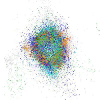
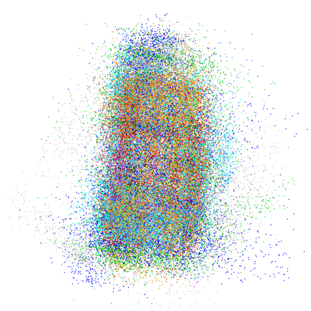
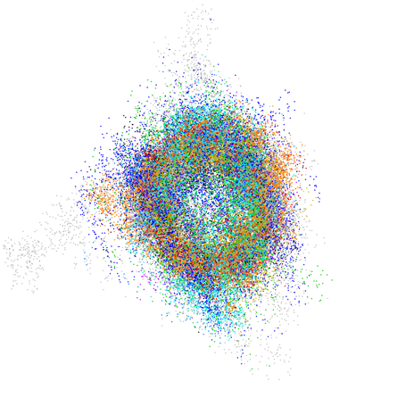
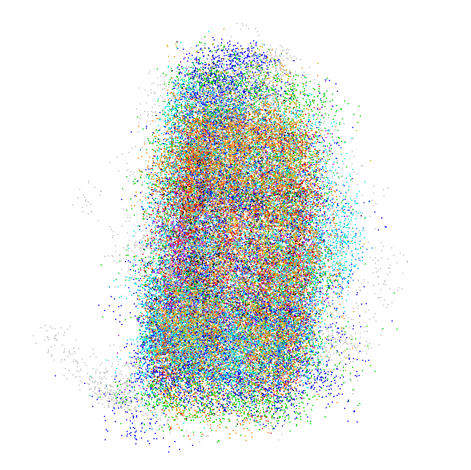
	(e)	(f)	(g)	(h)

Figure 9: Registered point clouds from the real data of Fig. 1. In the first two columns, we show the original point clouds, and in the last two columns, we show the cleaned point clouds obtained after post processing.

6 Conclusion

We presented a novel method to handle anisotropic and space-varying noise in the EM-GMM framework for point clouds registration. Unlike previous methods, we define an explicit Gaussian prior on the localization noise. We derived closed form updates for arbitrary anisotropic covariances at each step of our stochastic EM algorithm. Experimental results showed that our method outperforms the baseline approach [14] when the point clouds are corrupted with high anisotropic noise, both in terms of registration accuracy and GMM reconstruction. We also emphasize the practical interest of our method on real SMLM data, for which there is an urgent need of registration methods taking into account high localization uncertainty.

Appendix A Computation of $p({\overline{\mathbf{y}}_{ji}}|\theta)$

The term $p({\overline{\mathbf{y}}_{ji}}|\theta)=\int_{{\mathbf{y}}_{ji}}p(\overline{\mathbf{y}}_{ji}|{\mathbf{y}}_{ji})p({\mathbf{y}}_{ji}|\theta)d{\mathbf{y}}_{ji}$ can be written

$$\sum_{k=1}^{K}p_{k}\int_{{\mathbf{y}}_{ji}}p(\overline{\mathbf{y}}_{ji}|{\mathbf{y}}_{ji})p({\mathbf{y}}_{ji}|z_{ji}=k,\theta)d{\mathbf{y}}_{ji}=\sum_{k=1}^{K}p_{k}\int_{{\mathbf{y}}_{ji}}{\mathcal{N}}(\overline{\mathbf{y}}_{ji};{\mathbf{y}}_{ji},\overline{\boldsymbol{\Sigma}}_{ji}){\mathcal{N}}(\phi_{j}({\mathbf{y}}_{ji});\boldsymbol{\mu}_{k},\boldsymbol{\Sigma}_{k})d{\mathbf{y}}_{ji}$$ (30)

Using ${\mathcal{N}}(\overline{\mathbf{y}}_{ji};{\mathbf{y}}_{ji},\overline{\boldsymbol{\Sigma}}_{ji})={\mathcal{N}}(\phi_{j}(\overline{\mathbf{y}}_{ji});\phi_{j}({\mathbf{y}}_{ji}),\overline{\boldsymbol{\Sigma}}_{ji}^{{\mathbf{R}}_{j}})={\mathcal{N}}(\phi_{j}(\overline{\mathbf{y}}_{ji})-\phi_{j}({{\mathbf{y}}_{ji}});0,\overline{\boldsymbol{\Sigma}}_{ji}^{{\mathbf{R}}_{j}})$, where $\overline{\boldsymbol{\Sigma}}_{ji}^{{\mathbf{R}}_{j}}={\mathbf{R}}_{j}\overline{\boldsymbol{\Sigma}}_{ji}{\mathbf{R}}_{j}^{T}$, and with the change of variables ${{\mathbf{y}}}^{\prime}_{ji}=\phi_{j}({\mathbf{y}}_{ji})$, we get:

$$\begin{split}p({\overline{\mathbf{y}}_{ji}}|\theta)=\sum_{k=1}^{K}p_{k}\int_{{\mathbf{y}}^{\prime}_{ji}}{\mathcal{N}}(\phi_{j}(\overline{\mathbf{y}}_{ji})-{\mathbf{y}}^{\prime}_{ji};0,\overline{\boldsymbol{\Sigma}}_{ji}^{{\mathbf{R}}_{j}})\,{\mathcal{N}}({\mathbf{y}}^{\prime}_{ji};\boldsymbol{\mu}_{k},\boldsymbol{\Sigma}_{k})d{\mathbf{y}}^{\prime}_{ji}\end{split}$$ (31)

The expression of $p({\overline{\mathbf{y}}_{ji}}|\theta)$ in (6) can be obtained easily using properties related to the sum of two normally distributed random variables.

Appendix B Derivation of $Q(\theta,\theta^{(l)})$

From the definition of the complete-data likelihood (9), the auxiliary function defined in (8) writes

$$\begin{split}Q(\theta,\theta^{(l)})=\sum_{\mathbf{z}}\int_{\mathbb{{\mathbf{y}}}}p({\mathbf{y}},{\mathbf{z}}|\overline{\mathbf{y}},\theta^{(l)})\log(p(\bar{\mathbf{y}}|{\mathbf{y}}))d{\mathbf{y}}+\sum_{\mathbf{z}}\int_{\mathbb{{\mathbf{y}}}}p({\mathbf{y}},{\mathbf{z}}|\overline{\mathbf{y}},\theta^{(l)})\log(p({\mathbf{y}},{\mathbf{z}}|\theta)d{\mathbf{y}}.\end{split}$$ (32)

The first term in (32) does not depend on $\theta$ and the second one can be factorized using the same strategy than for the standard the GMM case [5]. We obtain

$$\begin{split}Q(\theta,\theta^{(l)})=(constant)+\sum_{jik}\Big{[}\int_{{\mathbf{y}}_{ji}}p({\mathbf{y}}_{ji},z_{ji}=k|\overline{\mathbf{y}}_{ji},\theta^{(l)})\log(p({\mathbf{y}}_{ji},z_{ji}=k|\theta)d{{{\mathbf{y}}_{ji}}}\Bigg{]}.\end{split}$$ (33)

Since $\alpha_{jik}\beta_{jik}({\mathbf{y}}_{ji})=p({\mathbf{y}}_{ji},z_{ji}=k|\overline{\mathbf{y}}_{ji},\theta^{(l)})$ (see ((11)), we get

$$\begin{split}Q(\theta,\theta^{(l)})=(constant)+\sum_{jik}\alpha_{jik}\Bigg{[}\int_{{\mathbf{y}}_{ji}}\beta_{jik}({\mathbf{y}}_{ji})\log(p({\mathbf{y}}_{ji},z_{ji}=k|\theta)d{{{\mathbf{y}}_{ji}}}\Bigg{]}\end{split}$$ (34)

To obtain the result (10), we use $p({\mathbf{y}}_{ji},z_{ji}=k|\theta)=p_{k}p({\mathbf{y}}_{ji}|z_{ji}=k,\theta)=p_{k}{\mathcal{N}}(\phi_{j}({\mathbf{y}}_{ji});\boldsymbol{\mu}_{k},\boldsymbol{\Sigma}_{k})$.

Appendix C Computation of $\beta_{jik}$

Using Bayes theorem, we have

$$\begin{split}\beta_{jik}({\mathbf{y}}_{ji})&\propto p(\overline{\mathbf{y}}_{ji}|{\mathbf{y}}_{ji})p({\mathbf{y}}_{ji}|z_{ji}=k,\theta^{(l)})\\ &\propto{\mathcal{N}}(\overline{\mathbf{y}}_{ji};{\mathbf{y}}_{ji},\overline{\boldsymbol{\Sigma}}_{ji}){\mathcal{N}}(\phi_{j}({\mathbf{y}}_{ji});\boldsymbol{\mu}_{k},\boldsymbol{\Sigma}_{k})\\ \end{split}$$

Since ${\mathcal{N}}(\overline{\mathbf{y}}_{ji};{\mathbf{y}}_{ji},\overline{\boldsymbol{\Sigma}}_{ji})={\mathcal{N}}(\phi_{j}(\overline{\mathbf{y}}_{ji});\phi_{j}({\mathbf{y}}_{ji}),\overline{\boldsymbol{\Sigma}}_{ji}^{{\mathbf{R}}_{j}})$ and ${\mathcal{N}}(a;b,c)={\mathcal{N}}(b+d;a+d,c)$, we can obtain easily

$$\begin{split}\beta_{jik}({\mathbf{y}}_{ji})\propto{\mathcal{N}}(\phi_{j}({\mathbf{y}}_{ji})-\boldsymbol{\mu}_{k};\phi_{j}(\overline{\mathbf{y}}_{ji})-\boldsymbol{\mu}_{k},\overline{\boldsymbol{\Sigma}}_{ji}^{{\mathbf{R}}_{j}})\,{\mathcal{N}}(\phi_{j}({\mathbf{y}}_{ji})-\boldsymbol{\mu}_{k};0,\boldsymbol{\Sigma}_{k}).\end{split}$$ (35)

We use the property ${\mathcal{N}}({\mathbf{x}};\boldsymbol{\mu}_{1},\boldsymbol{\Sigma}_{1}){\mathcal{N}}({\mathbf{x}};0,\boldsymbol{\Sigma}_{2})\propto{\mathcal{N}}(.;\boldsymbol{\mu}_{3},\boldsymbol{\Sigma}_{3})$ with $\boldsymbol{\mu}_{3}=\boldsymbol{\Sigma}_{2}(\boldsymbol{\Sigma}_{1}+\boldsymbol{\Sigma}_{2})^{-1}\boldsymbol{\mu}_{1}$, and $\boldsymbol{\Sigma}_{3}=\boldsymbol{\Sigma}_{1}(\boldsymbol{\Sigma}_{1}+\boldsymbol{\Sigma}_{2})^{-1}\boldsymbol{\Sigma}_{2}$, to obtain

$$\beta_{jik}({\mathbf{y}}_{ji})={\mathcal{N}}(\phi_{j}({\mathbf{y}}_{ji})-\boldsymbol{\mu}_{k};\hat{{\mathbf{y}}}_{ji}-\boldsymbol{\mu}_{k},\overline{\boldsymbol{\Sigma}}_{ji}^{{\mathbf{R}}_{j}}\left(\boldsymbol{\Sigma}_{k}+\overline{\boldsymbol{\Sigma}}_{ji}^{{\mathbf{R}}_{j}}\right)^{-1}\boldsymbol{\Sigma}_{k})$$ (36)

Finally, in order to obtain the result (14), we have to show that $({\mathbf{I}}-{\mathbf{W}}_{jik})=\overline{\boldsymbol{\Sigma}}_{ji}^{{\mathbf{R}}_{j}}\left(\boldsymbol{\Sigma}_{k}+\overline{\boldsymbol{\Sigma}}_{ji}^{{\mathbf{R}}_{j}}\right)^{-1}$. This can be obtained by writting ${\mathbf{I}}$ as $\left(\boldsymbol{\Sigma}_{k}+\overline{\boldsymbol{\Sigma}}_{ji}^{{\mathbf{R}}_{j}}\right)\left(\boldsymbol{\Sigma}_{k}+\overline{\boldsymbol{\Sigma}}_{ji}^{{\mathbf{R}}_{j}}\right)^{-1}$.

Appendix D Update of the GMM parameters

The update of the GMM parameters can be obtained by cancelling the derivative of $Q(\theta,\theta^{(l)}$) in (10).

Update of $p_{k}$  For the update of $p_{k}$, we also need to impose the constraint $\sum_{k}p_{k}=1$. To this end, we introduce the Lagrange multiplier $\lambda$ and solve the equation:

$$\begin{split}\frac{\partial}{\partial p_{k}}\Bigg{[}\sum_{ji}\Bigg{(}\alpha_{jik}\int_{{\mathbf{y}}_{ji}}\beta_{jik}({\mathbf{y}}_{ji})\log(p_{k})d{\mathbf{y}}_{ji}\Bigg{)}+\lambda\Bigg{(}\sum_{l=1}^{K}p_{l}-1\Bigg{)}\Bigg{]}=0\end{split}$$ (37)

Since $\int_{{\mathbf{y}}_{ji}}\beta_{jik}({\mathbf{y}}_{ji})d{\mathbf{y}}_{ji}=1$, we obtain directly the result (21). Update of $\boldsymbol{\mu}_{k}$  The cancellation of the derivative with respect to $\boldsymbol{\mu}_{k}$ yields

$$\sum_{ji}\alpha_{jik}\int_{{\mathbf{y}}_{ji}}\beta_{jik}({\mathbf{y}}_{ji})\boldsymbol{\Sigma}_{k}^{-1}(\phi_{j}({\mathbf{y}}_{ji})-\boldsymbol{\mu}_{k})d{\mathbf{y}}_{ji}=0$$ (38)

Since $\int_{{\mathbf{y}}_{ji}}\beta_{jik}({\mathbf{y}}_{ji})d{\mathbf{y}}_{ji}=1$, (38) writes

$$\sum_{ji}\alpha_{jik}\boldsymbol{\Sigma}_{k}^{-1}\left(\int_{{\mathbf{y}}_{ji}}\phi_{j}({\mathbf{y}}_{ji})\beta_{jik}({\mathbf{y}}_{ji})d{\mathbf{y}}_{ji}-\boldsymbol{\mu}_{k}\right)=0.$$ (39)

Using the notation $E[X]=\int_{y}\beta_{jik}(y)Xdy$, we get

$$\sum_{ji}\alpha_{jik}\boldsymbol{\Sigma}_{k}^{-1}\left(E[\phi_{j}({\mathbf{y}}_{ji})]-\boldsymbol{\mu}_{k}\right)=0.$$ (40)

with which we can easily solve to obtain the expected result (22). Update of $\boldsymbol{\Sigma}_{k}$  We rewrite (10) without the constant terms w.r.t. $\boldsymbol{\Sigma}_{k}$ (and follow the strategy desribed in [5] for the standard GMM case) to obtain

$$\begin{split}Q(\theta,\theta^{(l)})=-\frac{1}{2}\sum_{k}\Bigg{(}\log\left|\boldsymbol{\Sigma}_{k}\right|\sum_{ji}\alpha_{jik}+\sum_{ji}\alpha_{jik}\text{tr}\bigg{(}\boldsymbol{\Sigma}_{k}^{-1}\int_{{\mathbf{y}}_{ji}}\beta_{jik}({\mathbf{y}}_{ji})(\phi_{j}({\mathbf{y}}_{ji})-\boldsymbol{\mu}_{k})(\phi_{j}({\mathbf{y}}_{ji})-\boldsymbol{\mu}_{k})^{T}d{\mathbf{y}}_{ji}\bigg{)}\Bigg{)}\end{split}$$ (41)

Using the notation $E[X]=\int_{y}\beta_{jik}(y)Xdy$, and following [5], we can easily obtain the result (23). Derivation of Algorithm 2 We first need to compute $E[\phi_{j}({\mathbf{y}}_{ji})]$ and $E[(\phi_{j}({\mathbf{y}}_{ji})-\boldsymbol{\mu}_{k})(\phi_{j}({\mathbf{y}}_{ji})-\boldsymbol{\mu}_{k})^{T}]$. Based on (14), $E[\phi_{j}({\mathbf{y}}_{ji})]$ can be written

$$\int_{{\mathbf{y}}_{ji}}\phi_{j}({\mathbf{y}}_{ji}){\mathcal{N}}(\phi_{j}({\mathbf{y}}_{ji}));\hat{{\mathbf{y}}}_{ji},({\mathbf{I}}-{\mathbf{W}}_{jik})\boldsymbol{\Sigma}_{k}))d{\mathbf{y}}_{ji}$$ (42)

Using the change of variable ${\mathbf{y}}^{\prime}_{ji}=\phi_{j}({\mathbf{y}}_{ji})$, we get:

$$\begin{array}[]{lll}E[\phi_{j}({\mathbf{y}}_{ji})]&=&\int_{{\mathbf{y}}^{\prime}_{ji}}{\mathbf{y}}^{\prime}_{ji}{\mathcal{N}}({\mathbf{y}}^{\prime}_{ji};\hat{{\mathbf{y}}}_{ji},({\mathbf{I}}-{\mathbf{W}}_{jik})\boldsymbol{\Sigma}_{k}))d{\mathbf{y}}^{\prime}_{ji}\\ &=&\hat{{\mathbf{y}}}_{ji}.\end{array}$$ (43)

We can compute $E[\phi_{j}({\mathbf{y}}_{ji})\phi_{j}({\mathbf{y}}_{ji})^{T}]$ with the same change of variables to obtain

$$\int_{{\mathbf{y}}^{\prime}_{ji}}{\mathbf{y}}^{\prime}_{ji}{{\mathbf{y}}^{\prime}_{ji}}^{T}{\mathcal{N}}({\mathbf{y}}^{\prime}_{ji}|\hat{{\mathbf{y}}}_{ji},({\mathbf{I}}-{\mathbf{W}}_{jik})\boldsymbol{\Sigma}_{k}))d{\mathbf{y}}^{\prime}_{ji}=\hat{{\mathbf{y}}}_{ji}\hat{{\mathbf{y}}}_{ji}^{T}+({\mathbf{I}}-{\mathbf{W}}_{jik})\boldsymbol{\Sigma}_{k}$$ (44)

Then, we can then easily derive:

$$\begin{split}E[(\phi_{j}({\mathbf{y}}_{ji})-\boldsymbol{\mu}_{k})(\phi_{j}({\mathbf{y}}_{ji})-\boldsymbol{\mu}_{k})^{T}]=\hat{{\mathbf{y}}}_{ji}\hat{{\mathbf{y}}}_{ji}^{T}+({\mathbf{I}}-{\mathbf{W}}_{jik})\boldsymbol{\Sigma}_{k}-\boldsymbol{\mu}_{k}\hat{{\mathbf{y}}}_{ji}^{T}-\hat{{\mathbf{y}}}_{ji}^{T}\boldsymbol{\mu}_{k}+\boldsymbol{\mu}_{k}\boldsymbol{\mu}_{k}^{T}\end{split}$$ (45)

Plugging (45) into (23) and using the updated form of $\boldsymbol{\mu}_{k}$ (22), we obtain

$$\boldsymbol{\Sigma}_{k}=\frac{\sum_{j=1}^{M}\sum_{i=1}^{N_{j}}\alpha_{jik}\left(\hat{{\mathbf{y}}}_{ji}\hat{{\mathbf{y}}}_{ji}^{T}+({\mathbf{I}}-{\mathbf{W}}_{jik})\boldsymbol{\Sigma}_{k}\right)}{\sum_{j=1}^{M}\sum_{i=1}^{N_{j}}\alpha_{jik}}-\boldsymbol{\mu}_{k}\boldsymbol{\mu}_{k}^{T}.$$ (46)

We can then easily derive Alg. 2 from (21) and (22) with $E[\phi_{j}({\mathbf{y}}_{ji})]=\hat{{\mathbf{y}}}_{ji}$, and from (46).

References

- [1] Y. Aoki, H. Goforth, R. Arun Srivatsan, and S. Lucey. PointnetLK: Robust & efficient point cloud registration using pointnet. In Computer Vision and Pattern Recognition (CVPR), pages 7163–7172, 2019.
- [2] R. Balachandran and J.M. Fitzpatrick. Iterative solution for rigid-body point-based registration with anisotropic weighting. In Medical Imaging 2009: Visualization, Image-Guided Procedures, and Modeling, volume 7261, page 72613D. International Society for Optics and Photonics, 2009.
- [3] P.J. Besl and N.D. McKay. Method for registration of 3D shapes. In Sensor fusion IV: control paradigms and data structures, volume 1611, pages 586–606, 1992.
- [4] S. Billings and R. Taylor. Generalized iterative most likely oriented-point (G-IMLOP) registration. International journal of computer assisted radiology and surgery, 10(8):1213–1226, 2015.
- [5] J.A. Bilmes. A gentle tutorial of the em algorithm and its application to parameter estimation for gaussian mixture and hidden markov models. International Computer Science Institute, 4(510):126, 1998.
- [6] J. Broeken, H. Johnson, D.S. Lidke, S. Liu, R.P.J. Nieuwenhuizen, S. Stallinga, K.A. Lidke, and B. Rieger. Resolution improvement by 3D particle averaging in localization microscopy. Methods and applications in fluorescence, 3(1):014003, 2015.
- [7] G. Celeux. The SEM algorithm: a probabilistic teacher algorithm derived from the em algorithm for the mixture problem. Computational statistics quarterly, 2:73–82, 1985.
- [8] H. Chui and A. Rangarajan. A feature registration framework using mixture models. In Proceedings IEEE Workshop on Mathematical Methods in Biomedical Image Analysis. MMBIA-2000 (Cat. No. PR00737), pages 190–197. IEEE, 2000.
- [9] B. Combès and S. Prima. An efficient EM-ICP algorithm for non-linear registration of large 3D point sets. Computer Vision and Image Understanding, 191:102854, 2020.
- [10] A.P. Dempster, N.M. Laird, and D.B. Rubin. Maximum likelihood from incomplete data via the em algorithm. Journal of the Royal Statistical Society: Series B (Methodological), 39(1):1–22, 1977.
- [11] B. Eckart, K. Kim, and J. Kautz. Hgmr: Hierarchical gaussian mixtures for adaptive 3d registration. In Proceedings of the European Conference on Computer Vision (ECCV), pages 705–721, 2018.
- [12] B. Eckart, K. Kim, A. Troccoli, A. Kelly, and J. Kautz. MLMD: Maximum likelihood mixture decoupling for fast and accurate point cloud registration. In 2015 International Conference on 3D Vision, pages 241–249. IEEE, 2015.
- [13] R.S.J. Estépar, A. Brun, and C.F. Westin. Robust generalized total least squares iterative closest point registration. In International Conference on Medical Image Computing and Computer-Assisted Intervention, pages 234–241. Springer, 2004.
- [14] G.D. Evangelidis and R. Horaud. Joint alignment of multiple point sets with batch and incremental expectation-maximization. IEEE transactions on pattern analysis and machine intelligence, 40(6):1397–1410, 2017.
- [15] Y. Fan, S. Faisan, E. Baudrier, F. Zwettler, M. Sauer, and D. Fortun. Stacked pointnets for alignment of particles with cylindrical symmetry in single molecule localization microscopy. In 2021 IEEE 18th International Symposium on Biomedical Imaging (ISBI), pages 858–862. IEEE, 2021.
- [16] J.A. Fessler and A.O. Hero. Space-alternating generalized expectation-maximization algorithm. IEEE Transactions on Signal Processing, 42(10):2664–2677, 1994.
- [17] D. Fortun, P. Guichard, V. Hamel, C.O.S. Sorzano, N. Banterle, P. Gönczy, and M. Unser. Reconstruction from multiple particles for 3d isotropic resolution in fluorescence microscopy. IEEE transactions on medical imaging, 37(5):1235–1246, 2018.
- [18] S. Gold, A. Rangarajan, C.P. Lu, S. Pappu, and E. Mjolsness. New algorithms for 2D and 3D point matching: pose estimation and correspondence. Pattern recognition, 31(8):1019–1031, 1998.
- [19] S. Granger and X. Pennec. Multi-scale EM-ICP: A fast and robust approach for surface registration. In European Conference on Computer Vision, pages 418–432. Springer, 2002.
- [20] M. Heilemann, S. Van De Linde, M. Schüttpelz, R. Kasper, B. Seefeldt, A. Mukherjee, P. Tinnefeld, and M. Sauer. Subdiffraction-resolution fluorescence imaging with conventional fluorescent probes. Angewandte Chemie International Edition, 47(33):6172–6176, 2008.
- [21] J. Hermans, D. Smeets, D. Vandermeulen, and P. Suetens. Robust point set registration using EM-ICP with information-theoretically optimal outlier handling. In CVPR 2011, pages 2465–2472. IEEE, 2011.
- [22] H. Heydarian, M. Joosten, A. Przybylski, F. Schueder, R. Jungmann, B. Van Werkhoven, J. Keller-Findeisen, J. Ries, S. Stallinga, M. Bates, and B. Rieger. 3D particle averaging and detection of macromolecular symmetry in localization microscopy. Nature Communications, 12(1):1–9, 2021.
- [23] R. Horaud, F. Forbes, M. Yguel, G. Dewaele, and J. Zhang. Rigid and articulated point registration with expectation conditional maximization. IEEE Transactions on Pattern Analysis and Machine Intelligence, 33(3):587–602, 2011.
- [24] D.Q. Huynh. Metrics for 3D rotations: Comparison and analysis. J. Math. Imaging Vis., 35(2):155–164, 2009.
- [25] B. Jian and B.C. Vemuri. Robust point set registration using gaussian mixture models. IEEE transactions on pattern analysis and machine intelligence, 33(8):1633–1645, 2010.
- [26] M. Le Guennec, N. Klena, G. Aeschlimann, V. Hamel, and P. Guichard. Overview of the centriole architecture. Current Opinion in Structural Biology, 66:58–65, 2021.
- [27] M. Le Guennec, N. Klena, D. Gambarotto, M.H. Laporte, A.M. Tassin, H. Van den Hoek, P.S. Erdmann, M. Schaffer, L. Kovacik, S. Borgers, K.N. Goldie, H. Stahlberg, M. Bornens, J. Azimzadeh, B.D. Engel, V. Hamel, and P. Guichard. A helical inner scaffold provides a structural basis for centriole cohesion. Science advances, 6(7):eaaz4137, 2020.
- [28] L. Maier-Hein, A.M. Franz, T.R. Dos Santos, M. Schmidt, M. Fangerau, H.P. Meinzer, and J.M. Fitzpatrick. Convergent iterative closest-point algorithm to accomodate anisotropic and inhomogenous localization error. IEEE transactions on pattern analysis and machine intelligence, 34(8):1520–1532, 2011.
- [29] X.L. Meng and D.B. Rubin. Maximum likelihood estimation via the ECM algorithm: A general framework. Biometrika, 80(2):267–278, 1993.
- [30] Z. Min, J. Wang, J. Pan, and M.Q.H Meng. Generalized 3D point set registration with hybrid mixture models for computer-assisted orthopedic surgery: From isotropic to anisotropic positional error. IEEE Transactions on Automation Science and Engineering, 18(4):1679–1691, 2011.
- [31] A. Myronenko and X. Song. Point set registration: Coherent point drift. IEEE Transactions on Pattern Analysis and Machine Intelligence, 32(12):2262–2275, 2010.
- [32] N. Ohta and K. Kanatani. Optimal estimation of three-dimensional rotation and reliability evaluation. IEICE Transactinos on Information and Systems, 81(11):1247–1252, 1998.
- [33] A. Ozerov, M. Lagrange, and E. Vincent. Uncertainty-based learning of acoustic models from noisy data. Computer Speech & Language, 27(3):874–894, 2013.
- [34] N. Ravikumar, A. Gooya, S. Çimen, A.F. Frangi, and Z.A. Taylor. Group-wise similarity registration of point sets using student’s t-mixture model for statistical shape models. Medical image analysis, 44:156–176, 2018.
- [35] N. Ravikumar, A. Gooya, A.F. Frangi, and Z.A. Taylor. Generalised coherent point drift for group-wise registration of multi-dimensional point sets. In International Conference on Medical Image Computing and Computer-Assisted Intervention, pages 309–316. Springer, 2017.
- [36] D. Salas, A. Le Gall, J.B. Fiche, A. Valeri, Y. Ke, P. Bron, G. Bellot, and M. Nollmann. Angular reconstitution-based 3D reconstructions of nanomolecular structures from superresolution light-microscopy images. Proceedings of the National Academy of Sciences, 114(35):9273–9278, 2017.
- [37] M. Sauer. Localization microscopy coming of age: from concepts to biological impact. Journal of cell science, 126(16):3505–3513, 2013.
- [38] O. Sorkine. Least-squares rigid motion using SVD. Technical notes, 120(3):52, 2009.
- [39] Y. Wang and J.M. Solomon. Deep closest point: Learning representations for point cloud registration. In International Conference on Computer Vision (ICCV), October 2019.
- [40] G.C.G. Wei and M.A. Tanner. A monte carlo implementation of the em algorithm and the poor man’s data augmentation algorithms. Journal of the American statistical Association, 85(411):699–704, 1990.
- [41] Z.J. Yew and G.H. Lee. Rpm-net: Robust point matching using learned features. In Computer Vision and Pattern Recognition (CVPR), 2020.
- [42] J. Zhu, R. Guo, Z. Li, J. Zhang, and S. Pang. Registration of multi-view point sets under the perspective of expectation-maximization. IEEE Transactions on Image Processing, 29:9176–9189, 2020.
- [43] F.U. Zwettler, S. Reinhard, D. Gambarotto, T.D.M. Bell, V. Hamel, P. Guichard, and M. Sauer. Molecular resolution imaging by post-labeling expansion single-molecule localization microscopy (Ex-SMLM). Nature communications, 11(1):1–11, 2020.