Vision Transformer with Deformable Attention

Abstract

Transformers have recently shown superior performances on various vision tasks. The large, sometimes even global, receptive field endows Transformer models with higher representation power over their CNN counterparts. Nevertheless, simply enlarging receptive field also gives rise to several concerns. On the one hand, using dense attention e.g., in ViT, leads to excessive memory and computational cost, and features can be influenced by irrelevant parts which are beyond the region of interests. On the other hand, the sparse attention adopted in PVT or Swin Transformer is data agnostic and may limit the ability to model long range relations. To mitigate these issues, we propose a novel deformable self-attention module, where the positions of key and value pairs in self-attention are selected in a data-dependent way. This flexible scheme enables the self-attention module to focus on relevant regions and capture more informative features. On this basis, we present Deformable Attention Transformer, a general backbone model with deformable attention for both image classification and dense prediction tasks. Extensive experiments show that our models achieve consistently improved results on comprehensive benchmarks. Code is available at https://github.com/LeapLabTHU/DAT.

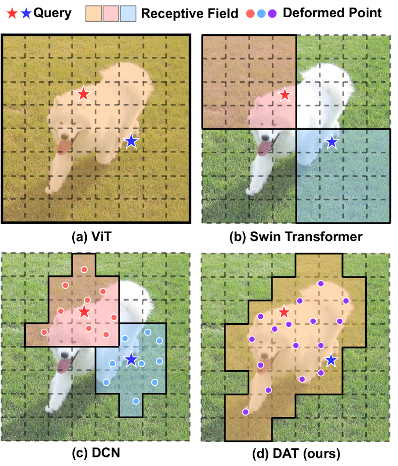
Figure 1: Comparison of DAT with other Vision Transformer models and DCN in CNN model. The red star and the blue star denote the different queries, and masks with solid line boundaries denote the regions to which the queries attend. In a data-agnostic way: (a) ViT [12] adopts full attention for all queries. (b) Swin Transformer [26] uses partitioned window attention. In a data-dependent way: (c) DCN [9] learns different deformed points for each query. (d) DAT learns shared deformed points for all queries.

1 Introduction

Transformer [34] is originally introduced to solve natural language processing tasks. It has recently shown great potential in the field of computer vision [12, 26, 36]. The pioneer work, Vision Transformer [12] (ViT), stacks multiple Transformer blocks to process non-overlapping image patch (i.e. visual token) sequences, leading to a convolution-free model for image classification. Compared to their CNN counterparts [18, 19], Transformer-based models have larger receptive fields and excel at modeling long-range dependencies, which are proved to achieve superior performance in the regime of a large amount of training data and model parameters. However, the superfluous attention in visual recognition is a double-edged sword, and has multiple drawbacks. Specifically, the excessive number of keys to attend per query patch yields high computational cost and slow convergence, and increases the risk of overfitting.

In order to avoid excessive attention computation, existing works [36, 26, 49, 11, 43, 6] have leveraged carefully designed efficient attention patterns to reduce the computation complexity. As two representative approaches among them, Swin Transformer [26] adopts window-based local attention to restrict attention in local windows, while Pyramid Vision Transformer (PVT) [36] downsamples the key and value feature maps to save computation. Though effective, the hand-crafted attention patterns are data-agnostic and may not be optimal. It is likely that relevant keys/values are dropped, while less important ones are still kept.

Ideally, one would expect that the candidate key/value set for a given query is flexible and has the ability to adapt to each individual input, such that the issues in hand-crafted sparse attention patterns can be alleviated. In fact, in the literature of CNNs, learning a deformable receptive field for the convolution filters has been shown effective in selectively attending to more informative regions on a data-dependent basis [9]. The most notable work, Deformable Convolution Networks [9], has yielded impressive results on many challenging vision tasks. This motivates us to explore a deformable attention pattern in Vision Transformers. However, a naive implementation of this idea leads to an unreasonably high memory/computation complexity: the overhead introduced by the deformable offsets is quadratic w.r.t the number of patches. As a consequence, although some recent work [54, 7, 46] have investigated the idea of deformable mechanism in Transformers , none of them have treated it as a basic building block for constructing a powerful backbone network like the DCN, due to the high computational cost. Instead, their deformable mechanism is either adopted in the detection head [54], or used as a pre-processing layer to sample patches for the subsequent backbone network [7].

In this paper, we present a simple and efficient deformable self-attention module, equipped with which a powerful pyramid backbone, named Deformable Attention Transformer (DAT), is constructed for image classification and various dense prediction tasks. Different from DCN that learns different offsets for different pixels in the whole feature map, we propose to learn a few groups of query agnostic offsets to shift keys and values to important regions (as illustrated in Figure 1(d)), based on the observation in [3, 52] that global attention usually results in the almost same attention patterns for different queries. This design both holds a linear space complexity and introduces a deformable attention pattern to Transformer backbones. Specifically, for each attention module, reference points are first generated as uniform grids, which are the same across the input data. Then, an offset network takes as input the query features and generates the corresponding offsets for all the reference points. In this way, the candidate keys/values are shifted towards important regions, thus augmenting the original self-attention module with higher flexibility and efficiency to capture more informative features.

To summarize, our contributions are as follows: we propose the first deformable self-attention backbone for visual recognition, where the data-dependent attention pattern endows higher flexibility and efficiency. Extensive experiments on ImageNet [10], ADE20K [51] and COCO [25] demonstrate that our model outperforms competitive baselines including Swin Transformer consistently, by a margin of 0.7 on the top-1 accuracy of image classification, 1.2 on the mIoU of semantic segmentation, 1.1 on object detection for both box AP and mask AP. The advantages on small and large objects are more distinct with a margin of 2.1.

2 Related Work

Transformer vision backbone. Since the introduction of ViT [12], improvements [36, 26, 49, 11, 43, 6, 28] have focused on learning multi-scale features for dense prediction tasks and efficient attention mechanisms. These attention mechanisms include windowed attention [26, 11], global tokens [6, 32, 21], focal attention [43] and dynamic token sizes [37]. More recently, convolution-based approaches have been introduced into Vision Transformer models. Among which exist researches focusing on complementing transformer models with convolution operations to introduce additional inductive biases. CvT [39] adopts convolution in the tokenization process and utilizes stride convolution to reduce the computation complexity of self-attention. ViT with convolutional stem [41] proposes to add convolutions at the early stage to achieve stabler training. CSwin Transformer [11] adopts a convolution-based positional encoding technique and shows improvements on downstream tasks. Many of these convolution-based techniques can potentially be applied on top of DAT for further performance improvements.

Deformable CNN and attention. Deformable convolution [9, 53] is a powerful mechanism to attend to flexible spatial locations conditioned on input data. Recently it has been applied to Vision Transformers [54, 7, 46]. Deformable DETR [54] improves the convergence of DETR [4] by selecting a small number of keys for each query on the top of a CNN backbone. Its deformable attention is not suited to a visual backbone for feature extraction as the lack of keys restricts representation power. Furthermore, the attention in Deformable DETR comes from simply learned linear projections and keys are not shared among query tokens. DPT [7] and PS-ViT [46] builds deformable modules to refine visual tokens. Specifically, DPT proposes a deformable patch embedding to refine patches across stages and PS-ViT introduces a spatial sampling module before a ViT backbone to improve visual tokens. None of them incorporate deformable attention into vision backbones. In contrast, our deformable attention takes a powerful and yet simple design to learn a set of global keys shared among visual tokens, and can be adopted as a general backbone for various vision tasks. Our method can also be viewed as a spatial adaptive mechanism, which has been proved effective in various works [38, 16].

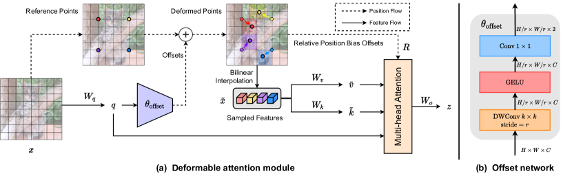
Figure 2: An illustration of our deformable attention mechanism. (a) presents the information flow of deformable attention. In the left part, a group of reference points is placed uniformly on the feature map, whose offsets are learned from the queries by the offset network. Then the deformed keys and values are projected from the sampled features according to the deformed points, as shown in the right part. Relative position bias is also computed by the deformed points, enhancing the multi-head attention which outputs the transformed features. We show only 4 reference points for a clear presentation, there are many more points in real implementation de facto. (b) reveals the detailed structure of the offset generation network, marked with sizes of feature maps.

3 Deformable Attention Transformer

3.1 Preliminaries

We first revisit the attention mechanism in recent Vision Transformers. Taking a flattened feature map $x\in\mathbb{R}^{N\times{}C}$ as the input, a multi-head self-attention (MHSA) block with $M$ heads is formulated as

$$q=xW_{q},\ k=xW_{k},\ v=xW_{v},$$ (1)

$$z^{(m)}=\sigma(q^{(m)}k^{(m)\top}/\sqrt{d})v^{(m)},m\!=\!1,\ldots,M,$$ (2)

$$z=\text{Concat}\left(z^{(1)},\ldots,z^{(M)}\right)W_{o},$$ (3)

where $\sigma(\cdot)$ denotes the softmax function, and $d\!=\!C/M$ is the dimension of each head. $z^{(m)}$ denotes the embedding output from the $m$-th attention head, $q^{(m)},k^{(m)},v^{(m)}\in\mathbb{R}^{N\times{}d}$ denote query, key, and value embeddings respectively. $W_{q},W_{k},W_{v},W_{o}\in\mathbb{R}^{C\times{}C}$ are the projection matrices. To build up a Transformer block, an MLP block with two linear transformations and a GELU activation is usually adopted to provide nonlinearity.

With normalization layers and identity shortcuts, the $l$-th Transformer block is formulated as

$$z_{l}^{\prime} =\text{MHSA}\left(\text{LN}(z_{l-1})\right)+z_{l-1},$$ (4)

$$z_{l} =\text{MLP}\left(\text{LN}(z_{l}^{\prime})\right)+z_{l}^{\prime},$$ (5)

where LN is Layer Normalization [1].

3.2 Deformable Attention

Existing hierarchical Vision Transformers, notably PVT [36] and Swin Transformer [26] try to address the challenge of excessive attention. The downsampling technique of the former results in severe information loss, and the shift-window attention of the latter leads to a much slower growth of receptive fields, which limits the potential of modeling large objects. Thus a data-dependent sparse attention is required to flexibly model relevant features, leading to deformable mechanism firstly proposed in DCN [9]. However, simply implementing DCN in Transformer models is a non-trivial problem. In DCN, each element on the feature map learns its offsets individually, of which a $3\!\times{}\!3$ deformable convolution on an $H\!\times{}\!W\!\times{}\!C$ feature map has the space complexity of $9HWC$. If we directly apply the same mechanism in the attention module, the space complexity will drastically rise to $N_{\text{q}}N_{\text{k}}C$, where $N_{\text{q}},N_{\text{k}}$ are the number of queries and keys and usually have the same scale as the feature map size $HW$, bringing approximately a biquadratic complexity. Although Deformable DETR [54] has managed to reduce this overhead by setting a lower number of keys with $N_{\text{k}}\!=\!4$ at each scale and works well as a detection head, it is inferior to attend to such few keys in a backbone network because of the unacceptable loss of information (see detailed comparison in Appendix). In the meantime, the observations in [52, 3] have revealed that different queries have similar attention maps in visual attention models. Therefore, we opt for a simpler solution with shared shifted keys and values for each query to achieve an efficient trade-off.

Specifically, we propose deformable attention to model the relations among tokens effectively under the guidance of the important regions in the feature maps. These focused regions are determined by multiple groups of deformed sampling points which are learned from the queries by an offset network. We adopt bilinear interpolation to sample features from the feature maps, and then the sampled features are fed to the key and value projections to get the deformed keys and values. Finally, standard multi-head attention is applied to attend queries to the sampled keys and aggregate features from the deformed values. Additionally, the locations of deformed points provide a more powerful relative position bias to facilitate the learning of the deformable attention, which will be discussed in the following sections.

Deformable attention module. As illustrated in Figure 2(a), given the input feature map $x\in\mathbb{R}^{H\times{}W\times{}C}$, a uniform grid of points $p\in\mathbb{R}^{H_{G}\times{}W_{G}\times{}2}$ are generated as the references. Specifically, the grid size is downsampled from the input feature map size by a factor $r$, $H_{G}=H/r,W_{G}=W/r$. The values of reference points are linearly spaced 2D coordinates $\{(0,0),\ldots,(H_{G}-1,W_{G}-1)\}$, and then we normalize them to the range $[-1,+1]$ according to the grid shape $H_{G}\times{}W_{G}$, in which $(-1,-1)$ indicates the top-left corner and $(+1,+1)$ indicates the bottom-right corner. To obtain the offset for each reference point, the feature maps are projected linearly to the query tokens $q\!=\!xW_{q}$, and then fed into a light weight sub-network $\theta_{\text{offset}}(\cdot)$ to generate the offsets $\Delta{}p=\theta_{\text{offset}}(q)$. To stabilize the training process, we scale the amplitude of $\Delta{}p$ by some predefined factor $s$ to prevent too large offset, i.e., $\Delta{}p\!\xleftarrow{}\!s\tanh{(\Delta{}p)}$. Then the features are sampled at the locations of deformed points as keys and values, followed by projection matrices:

$$q= xW_{q},\ \tilde{k}=\tilde{x}W_{k},\ \tilde{v}=\tilde{x}W_{v},$$ (6)

with $$\Delta{}p=\theta_{\text{offset}}(q),\ \tilde{x}=\phi(x;p+\Delta{}p).$$ (7)

$\tilde{k}$ and $\tilde{v}$ represent the deformed key and value embeddings respectively. Specifically, we set the sampling function $\phi(\cdot;\cdot)$ to a bilinear interpolation to make it differentiable:

$$\phi\left(z;(p_{x},p_{y})\right)\!=\!\sum_{(r_{x},r_{y})}\!g(p_{x},r_{x})g(p_{y},r_{y})z[r_{y},r_{x},:],$$ (8)

where $g(a,b)=\max(0,1-|a-b|)$ and $(r_{x},r_{y})$ indexes all the locations on $z\!\in\!\mathbb{R}^{H\times{}W\times{}C}$. As $g$ would be non-zero only on the 4 integral points closest to $(p_{x},p_{y})$, it simplifies Eq.(8) to a weighted average on 4 locations. Similar to existing approaches, we perform multi-head attention on $q,k,v$ and adopt relative position offsets $R$. The output of an attention head is formulated as:

$$z^{(m)}=\sigma\left(q^{(m)}\tilde{k}^{(m)\top}/\sqrt{d}+\phi(\hat{B};R)\right)\tilde{v}^{(m)},$$ (9)

where $\phi(\hat{B};R)\in\mathbb{R}^{HW\times{}H_{G}W_{G}}$ correspond to the position embedding following previous work [26] while with several adaptations. Details will be explained later in this section. Features of each head are concatenated together and projected through $W_{o}$ to get the final output $z$ as Eq.(3).

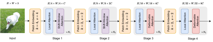
Figure 3: An illustration of DAT architecture. $N_{1}$ to $N_{4}$ are the numbers of stacked successive local attention and shift-window / deformable attention blocks. $k$ and $s$ denote the kernel size and stride of the convolution layer in patch embeddings.

Offset generation. As we have stated, a sub-network is adopted for offset generation which consumes the query features and outputs the offset values for reference points respectively. Considering that each reference point covers a local $s\times s$ region ($s$ is the largest value for offset), the generation network should also have the perception of the local features to learn reasonable offsets. Therefore, we implement the sub-network as two convolution modules with a nonlinear activation, as depicted in Figure 2(b). The input features are first passed through a $5\!\times\!5$ depthwise convolution to capture local features. Then, GELU activation and a $1\!\times\!1$ convolution is adopted to get the 2D offsets. It is also worth noticing that the bias in $1\times{}1$ convolution is dropped to alleviate the compulsive shift for all locations.

Offset groups. To promote the diversity of the deformed points, we follow a similar paradigm in MHSA, and split the feature channel into $G$ groups. Features from each group use the shared sub-network to generate the corresponding offsets respectively. In practice, the head number $M$ for the attention module is set to be multiple times of the size of offset groups $G$, ensuring that multiple attention heads are assigned to one group of deformed keys and values.

Deformable relative position bias. Relative position bias encodes the relative positions between every pair of query and key, which augments the vanilla attention with spatial information. Considering a feature map with shape $H\!\times{}\!W$, its relative coordinate displacements lie in the range of $[-H,H]$ and $[-W,W]$ at two dimensions respectively. In Swin Transformer [26], a relative position bias table $\hat{B}\in\mathbb{R}^{(2H-1)\times{}(2W-1)}$ is constructed to obtain the relative position bias $B$ by indexing the table with the relative displacements in two directions. Since our deformable attention has continuous positions of keys, we compute the relative displacements in the normalized range $[-1,+1]$, and then interpolate $\phi(\hat{B};R)$ in the parameterized bias table $\hat{B}\in\mathbb{R}^{(2H-1)\times{}(2W-1)}$ by the continuous relative displacements in order to cover all possible offset values.

Computational complexity. Deformable multi-head attention (DMHA) has a similar computation cost as the counterpart in PVT or Swin Transformer. The only additional overhead comes from the sub-network that is used to generate offsets. The complexity of the whole module can be summarized as:

$$\Omega(\text{DMHA})\!=\!\underbrace{2HWN_{\text{s}}C\!\!+\!\!2HWC^{2}\!\!+\!\!2N_{\text{s}}C^{2}}_{\text{vanilla self-attention module}}\!+\!\underbrace{(k^{2}\!+\!2)N_{\text{s}}C}_{\text{{\color[rgb]{0,0,1}offset network}}},$$ (10)

where $N_{\text{s}}\!=\!H_{G}W_{G}\!=\!HW/r^{2}$ is the number of sampled points. It can be immediately seen that the computational cost of the offset network has linear complexity w.r.t. the channel size, which is comparably minor to the cost for attention computation. Typically, consider the third stage of a Swin-T [26] model for image classification where $H\!=\!W\!=\!14$, $N_{s}\!=\!49$, $C\!=\!384$, the computational cost for the attention module in a single block is 79.63M FLOPs. If equipped with our deformable module (with $k\!=\!5$), the additional overhead is 5.08M Flops, which is only $6.0\%$ of the whole module. Additionally, by choosing a large downsample factor $r$, the complexity will be further reduced, which makes it friendly to the tasks with much higher resolution inputs such as object detection and instance segmentation.

3.3 Model Architectures

We replace the vanilla MHSA with our deformable attention in the Transformer (Eq.(4)), and combine it with an MLP (Eq.(5)) to build a deformable vision transformer block. In terms of the network architecture, our model, Deformable Attention Transformer, shares a similar pyramid structure with [36, 26, 7, 31], which is broadly applicable to various vision tasks requiring multiscale feature maps. As illustrated in Figure 3, an input image with shape $H\times{}W\times{}3$ is firstly embedded by a 4$\times{}$4 non-overlapped convolution with stride 4, followed by a normalization layer to get the $\frac{H}{4}\times{}\frac{W}{4}\times{}C$ patch embeddings. Aiming to build a hierarchical feature pyramid, the backbone includes 4 stages with a progressively increasing stride. Between two consecutive stages, there is a non-overlapped 2$\times{}$2 convolution with stride 2 to downsample the feature map to halve the spatial size and double the feature dimensions. In classification task, we first normalize the feature maps output from the last stage and then adopt a linear classifier with pooled features to predict the logits. In object detection, instance segmentation and semantic segmentation tasks, DAT plays the role of a backbone in an integrated vision model to extract multiscale features. We add a normalization layer to the features from each stage before feeding them into the following modules such as FPN [23] in object detection or decoders in semantic segmentation.

We introduce successive local attention and deformable attention blocks in the third and the fourth stage of DAT. The feature maps are firstly processed by a window-based local attention to aggregate information locally, and then passed through the deformable attention block to model the global relations between the local augmented tokens. This alternate design of attention blocks with local and global receptive fields helps the model learn strong representations, sharing a similar pattern in GLiT [5], TNT [15] and Pointformer [29]. Since the first two stages mainly learn local features, deformable attention in these early stages is less preferred. In addition, the keys and values in the first two stages have a rather large spatial size, which greatly increase the computational overhead in the dot products and bilinear interpolations in deformable attention. Therefore, to achieve a trade-off between model capacity and computational burden, we only place deformable attention in the third and the fourth stage and adopt the shift-window attention in Swin Transformer [26] to have a better representation in the early stages. We build three variants of DAT in different parameters and FLOPs for a fair comparison with other Vision Transformer models. We change the model size by stacking more blocks in the third stage and increasing the hidden dimensions. The detailed architectures are reported in Table 1. Note that there are other design choices for the first two stages of DAT, e.g., the SRA module in PVT. We show the comparison results in Table 7.

DAT Architectures
	DAT-T	DAT-S	DAT-B
$\begin{matrix}\text{Stage 1}\\ (\text{56}\!\times{}\!\text{56})\end{matrix}$	$N_{1}\!=\!1,C\!=\!96$	$N_{1}\!=\!1,C\!=\!96$	$N_{1}\!=\!1,C\!=\!128$
	window size: 7	window size: 7	window size: 7
	heads: 3	heads: 3	heads: 4
$\begin{matrix}\text{Stage 2}\\ (\text{28}\!\times{}\!\text{28})\end{matrix}$	$N_{2}\!=\!1,C\!=\!192$	$N_{2}\!=\!1,C\!=\!192$	$N_{2}\!=\!1,C\!=\!256$
	window size: 7	window size: 7	window size: 7
	heads: 6	heads: 6	heads: 8
$\begin{matrix}\text{Stage 3}\\ (\text{14}\!\times{}\!\text{14})\end{matrix}$	$N_{3}\!=\!3,C\!=\!384$	$N_{3}\!=\!9,C\!=\!384$	$N_{3}\!=\!9,C\!=\!512$
	window size: 7	window size: 7	window size: 7
	heads: 12	heads: 12	heads: 16
	groups: 3	groups: 3	groups: 4
$\begin{matrix}\text{Stage 4}\\ (\text{7}\!\times{}\!\text{7})\end{matrix}$	$N_{4}\!=\!1,C\!=\!768$	$N_{4}\!=\!1,C\!=\!768$	$N_{4}\!=\!1,C\!=\!1024$
	window size: 7	window size: 7	window size: 7
	heads: 24	heads: 24	heads: 32
	groups: 6	groups: 6	groups: 8

Table 1: Model architecture specifications. $\bm{N_{i}}$: Number of block at stage i. $\bm{C}$: Channel dimension. window size: Region size in local attention module. heads: Number of heads in DMHA. groups: Offset groups in DMHA.

4 Experiments

We conduct experiments on several datasets to verify the effectiveness of our proposed DAT. We show our results on ImageNet-1K [10] classification, COCO [25] object detection and ADE20K [51] semantic segmentation tasks. In addition, we provide ablation studies and visualizations to further show the effectiveness of our method.

4.1 ImageNet-1K Classification

ImageNet-1K [10] dataset has 1.28M images for training and 50K images for validation. We train three variants of DAT on the training split and report the Top-1 accuracy on the validation split to compare with other Vision Transformer models.

We use AdamW [27] optimizer to train our models for 300 epochs with a cosine learning rate decay. The basic learning rate for a batch size of 1024 is set to $1\times 10^{-3}$, and then linearly scaled w.r.t. the batch size. To stabilize training procedures, we schedule a linear warm-up of learning rate from $1\times 10^{-6}$ to the basic learning rate, and for a better convergence the cosine decay rule is applied to gradually decrease the learning rate to $1\times 10^{-7}$ during training. We follow DeiT [33] to set the advanced data augmentation, including RandAugment [8], Mixup [48] and CutMix [47] to avoid overfitting. In addition, stochastic depth [20] and weight decay of 0.05 are also applied, in which the stochastic depth degree is chosen 0.2, 0.3 and 0.5 for the tiny, small and base model, respectively. We do not adopt EMA [30], random erasing [50] and the vanilla drop out, which does not improve the training of Vision Transformers, as verified in [33, 26]. In terms of larger resolution finetuning, we finetune our DAT-B using AdamW optimizer with a cosine scheduled learning rate $4\times{}10^{-6}$ for 30 epochs. We set the stochastic depth rate to 0.5 and lower the weight decay to $1\times{}10^{-8}$ to keep the regularization.

We report our results in Table 2, with 300 training epochs. Compared with other state-of-the-art Vision Transformers, our DATs achieve significant improvements on the Top-1 accuracy with similar computational complexities. Our method DAT outperforms Swin Transformer [26], PVT [36], DPT [7] and DeiT [33] in all three scales. Without inserting convolutions in Transformer blocks [35, 13, 14], or using overlapped convolutions in patch embeddings [6, 11, 45], DATs achieve gains of +0.7, +0.7 and +0.5 over Swin Transformer [26] counterparts. When finetuning at $384\times{}384$ resolution, our model continues performing better than Swin Transformer by 0.3.

ImageNet-1K Classification
Method	Resolution	FLOPs	#Param	Top-1 Acc.
DeiT-S [33]	$\text{224}^{\text{2}}$	4.6G	22M	79.8
PVT-S [36]	$\text{224}^{\text{2}}$	3.8G	25M	79.8
GLiT-S [5]	$\text{224}^{\text{2}}$	4.4G	25M	80.5
DPT-S [7]	$\text{224}^{\text{2}}$	4.0G	26M	81.0
Swin-T [26]	$\text{224}^{\text{2}}$	4.5G	29M	81.3
DAT-T	$\text{224}^{\text{2}}$	4.6G	29M	82.0 (+0.7)
PVT-M [36]	$\text{224}^{\text{2}}$	6.9G	46M	81.2
PVT-L [36]	$\text{224}^{\text{2}}$	9.8G	61M	81.7
DPT-M [7]	$\text{224}^{\text{2}}$	6.9G	46M	81.9
Swin-S [26]	$\text{224}^{\text{2}}$	8.8G	50M	83.0
DAT-S	$\text{224}^{\text{2}}$	9.0G	50M	83.7 (+0.7)
DeiT-B [33]	$\text{224}^{\text{2}}$	17.5G	86M	81.8
GLiT-B [5]	$\text{224}^{\text{2}}$	17.0G	96M	82.3
Swin-B [26]	$\text{224}^{\text{2}}$	15.5G	88M	83.5
DAT-B	$\text{224}^{\text{2}}$	15.8G	88M	84.0 (+0.5)
DeiT-B [33]	$\text{384}^{\text{2}}$	55.4G	86M	83.1
Swin-B [26]	$\text{384}^{\text{2}}$	47.2G	88M	84.5
DAT-B	$\text{384}^{\text{2}}$	49.8G	88M	84.8 (+0.3)

Table 2: Comparisons of DAT with other vision transformer backbones on FLOPs, parameters, accuracy on the ImageNet-1K classification task.

RetinaNet Object Detection on COCO
Method	FLOPs	#Param	Sch.	AP	AP${}_{\text{50}}$	AP${}_{\text{75}}$	APs	APm	APl
PVT-S	286G	34M	1x	40.4	61.3	43.0	25.0	42.9	55.7
Swin-T	248G	38M	1x	41.7	63.1	44.3	27.0	45.3	54.7
DAT-T	253G	38M	1x	42.8	64.4	45.2	28.0	45.8	57.8
PVT-S	286G	34M	3x	42.3	63.1	44.8	26.7	45.1	57.2
Swin-T	248G	38M	3x	44.8	66.1	48.0	29.2	48.6	58.6
DAT-T	253G	38M	3x	45.6	67.2	48.5	31.3	49.1	60.8
Swin-S	339G	60M	1x	44.5	66.1	47.4	29.8	48.5	59.1
DAT-S	359G	60M	1x	45.7	67.7	48.5	30.5	49.3	61.3
Swin-S	339G	60M	3x	47.3	68.6	50.8	31.9	51.8	62.1
DAT-S	359G	60M	3x	47.9	69.6	51.2	32.3	51.8	63.4

Table 3: Results on COCO object detection with RetinaNet [24]. The table displays the number of parameters, computational cost (FLOPs), mAP at different mIoU thresholds and different object sizes. The FLOPs are computed over backbone, FPN and detection head with RGB input image at the resolution of 1280$\times$800.

(a) Mask R-CNN Object Detection & Instance Segmentation on COCO
Method	FLOPs	#Param	Schedule	APb	AP${}^{b}_{\text{50}}$	AP${}^{b}_{\text{75}}$	AP${}^{b}_{s}$	AP${}^{b}_{m}$	AP${}^{b}_{l}$	APm	AP${}^{m}_{\text{50}}$	AP${}^{m}_{\text{75}}$	AP${}^{m}_{s}$	AP${}^{m}_{m}$	AP${}^{m}_{l}$
Swin-T	267G	48M	1x	43.7	66.6	47.7	28.5	47.0	57.3	39.8	63.3	42.7	24.2	43.1	54.6
DAT-T	272G	48M	1x	44.4	67.6	48.5	28.3	47.5	58.5	40.4	64.2	43.1	23.9	43.8	55.5
Swin-T	267G	48M	3x	46.0	68.1	50.3	31.2	49.2	60.1	41.6	65.1	44.9	25.9	45.1	56.9
DAT-T	272G	48M	3x	47.1	69.2	51.6	32.0	50.3	61.0	42.4	66.1	45.5	27.2	45.8	57.1
Swin-S	359G	69M	1x	45.7	67.9	50.4	29.5	48.9	60.0	41.1	64.9	44.2	25.1	44.3	56.6
DAT-S	378G	69M	1x	47.1	69.9	51.5	30.5	50.1	62.1	42.5	66.7	45.4	25.5	45.8	58.5
Swin-S	359G	69M	3x	48.5	70.2	53.5	33.4	52.1	63.3	43.3	67.3	46.6	28.1	46.7	58.6
DAT-S	378G	69M	3x	49.0	70.9	53.8	32.7	52.6	64.0	44.0	68.0	47.5	27.8	47.7	59.5
(b) Cascade Mask R-CNN Object Detection & Instance Segmentation on COCO
Method	FLOPs	#Param	Schedule	APb	AP${}^{b}_{\text{50}}$	AP${}^{b}_{\text{75}}$	AP${}^{b}_{s}$	AP${}^{b}_{m}$	AP${}^{b}_{l}$	APm	AP${}^{m}_{\text{50}}$	AP${}^{m}_{\text{75}}$	AP${}^{m}_{s}$	AP${}^{m}_{m}$	AP${}^{m}_{l}$
Swin-T	745G	86M	1x	48.1	67.1	52.2	30.4	51.5	63.1	41.7	64.4	45.0	24.0	45.2	56.9
DAT-T	750G	86M	1x	49.1	68.2	52.9	31.2	52.4	65.1	42.5	65.4	45.8	25.2	45.9	58.6
Swin-T	745G	86M	3x	50.4	69.2	54.7	33.8	54.1	65.2	43.7	66.6	47.3	27.3	47.5	59.0
DAT-T	750G	86M	3x	51.3	70.1	55.8	34.1	54.6	66.9	44.5	67.5	48.1	27.9	47.9	60.3
Swin-S	838G	107M	3x	51.9	70.7	56.3	35.2	55.7	67.7	45.0	68.2	48.8	28.8	48.7	60.6
DAT-S	857G	107M	3x	52.7	71.7	57.2	37.3	56.3	68.0	45.5	69.1	49.3	30.2	49.2	60.9
Swin-B	982G	145M	3x	51.9	70.5	56.4	35.4	55.2	67.4	45.0	68.1	48.9	28.9	48.3	60.4
DAT-B	1003G	145M	3x	53.0	71.9	57.6	36.0	56.8	69.1	45.8	69.3	49.5	29.2	49.5	61.9

Table 4: Results on COCO object detection and instance segmentation. The table displays the number of parameters, computational cost (FLOPs), mAP at different IoU thresholds and mAP for objects in different sizes. The FLOPs are computed over backbone, FPN and detection head with RGB input image at the resolution of 1280$\times$800.

4.2 COCO Object Detection

COCO [25] object detection and instance segmentation dataset has 118K training images and 5K validation images. We use our DAT as the backbone in RetinaNet [24], Mask R-CNN [17] and Cascade Mask R-CNN [2] frameworks to evaluate the effectiveness of our method. We pretrain our models on ImageNet-1K dataset for 300 epochs and follow the similar training strategies in Swin Transformer [26] to compare our methods fairly.

We report our DAT on RetinaNet model in 1x and 3x training schedules. As shown in Table 3, DAT outperforms Swin Transformer by 1.1 and 1.2 mAP among tiny and small models. When implemented in two-stage detectors, e.g., Mask R-CNN and Cascade Mask R-CNN, our model achieves consistent improvements over Swin Transformer models in different sizes, as shown in Table 4. We can see that DAT achieves most improvements on large objects (up to +2.1) due to the flexibility in modeling long-range dependencies. The gaps for small objects detection and instance segmentation are also pronounced (up to +2.1), which shows that DATs also have the capacity of modeling relations in the local region.

4.3 ADE20K Semantic Segmentation

ADE20K [51] is a popular dataset for semantic segmentation with 20K training images and 2K validation images. We employ our DAT on two widely adopted segmentation models, SemanticFPN [22] and UperNet [40]. To make a fair comparison to PVT [36] and Swin Transformer [26], we follow the learning rate schedules and training epochs, except for the degree of stochastic depth, which is a key hyper-parameter affecting the final performance. We set it for 0.3, 0.3 and 0.5 for tiny, small and base variants of our DAT respectively for both two models. With the pretraining models on ImageNet-1K, we train SemanticFPN for 40k steps and UperNet for 160k steps. In Table 5, we report the results on the validation set with the highest mIoU score of all methods. In comparison with PVT [36], our tiny model outperforms PVT-S by +0.5 mIoU even with less FLOPs and achieves a sharp boost with +3.1 and +2.5 in mIoU with a slightly larger model size. Our DAT has a significant improvement over the Swin Transformer at each of three model scales, with +1.0, +0.7 and +1.2 in mIoU respectively, showing our method’s effectiveness.

4.4 Ablation Study

In this section, we ablate the key components in our DAT to verify the effectiveness of these designs. We report the results on ImageNet-1K classification based on DAT-T.

Geometric information exploitation. We first evaluate the effectiveness of our proposed deformable offsets and deformable relative position embeddings, as shown in Table 6. Either adopting offsets in feature sampling or using deformable relative position embedding provides +0.3 improvement. We also try other types of position embeddings, including a fixed learnable position bias and a depth-wise convolution in [11]. But none of them is effective with only +0.1 gain over that without position embedding, which shows our deformable relative position bias is more compatible with deformable attention. There is also an observation from rows 6 and 7 in Table 6 that our model can adapt to different attention modules at the first two stages and achieve competitive results. Our model with SRA [36] at the first two stages outperforms PVT-M by 0.5 with 65$\%$ FLOPs.

Deformable attention at different stages. We replace the shift-window attention of Swin Transfomer [26] with our deformable attention at different stages. As shown in Table 7, only replacing the attention in the last stage improves by 0.1 and replacing the last two stages leads to a performance gain of 0.7 (achieving an overall accuracy of 82.0). However, replacing with more deformable attention at the early stages slightly decreases the accuracy.

Semantic Segmentation on ADE20K
Backbone	Method	FLOPs	#Params	mIoU	mAcc	mIoU†
PVT-S	S-FPN	225G	28M	41.95	53.02	41.95
DAT-T	S-FPN	198G	32M	42.56	54.72	44.22
PVT-M	S-FPN	315G	48M	42.91	53.80	43.34
DAT-S	S-FPN	320G	53M	46.08	58.17	48.46
PVT-L	S-FPN	420G	65M	43.49	54.62	43.92
DAT-B	S-FPN	481G	92M	47.02	59.47	49.01
Swin-T	UperNet	945G	60M	44.51	55.61	45.81
DAT-T	UperNet	957G	60M	45.54	57.95	46.44
Swin-S	UperNet	1038G	81M	47.64	58.78	49.47
DAT-S	UperNet	1079G	81M	48.31	60.44	49.84
Swin-B	UperNet	1188G	121M	48.13	59.13	49.72
DAT-B	UperNet	1212G	121M	49.38	61.82	50.55

Table 5: Results of semantic segmentation. The FLOPs are computed over encoders and decoders with RGB input image at the resolution of 512$\times$2048. $\dagger$ denotes the metrics are reported under a multi-scale test setting with flip augmentation. S-FPN is short for SemanticFPN [22] model. The results of PVT and Swin Transformer are copied from their Github repositories, which are higher than the versions in their original papers.

Attn.	Offsets	Pos. Emebd	FLOPs	#Param	Acc.	Diff.
S	✗	✗	4.57G	28.29M	81.4	-0.6
S	✗	Relative	4.57G	28.32M	81.7	-0.3
S	✓	✗	4.58G	28.29M	81.7	-0.3
S	✓	Fixed	4.58G	29.73M	81.8	-0.2
S	✓	DWConv	4.59G	28.31M	81.8	-0.2
P	✓	Relative	4.48G	30.68M	81.7	-0.3
S	✓	Relative	4.59G	28.32M	82.0	DAT

Table 6: Ablation study on different ways to exploiting geometric information. P represents the first two stages use SRA attention in [36], and S represents shift-window attention in [26]. ✓ in offsets means performing spatial sampling in deformable attention module while ✗ means not.

Stages w/ Deformable Attention					FLOPs	#Param	Acc.
Stage 1	Stage 2	Stage 3	Stage 4
✓	✓	✓	✓	4.64G	28.39M	81.7
	✓	✓	✓	4.60G	28.34M	81.9
		✓	✓	4.59G	28.32M	82.0
			✓	4.51G	28.29M	81.4
Swin-T [26]				4.51G	28.29M	81.3

Table 7: Ablation study on applying deformable attention on different stages. ✓ means this stage is made up of successive local attention and deformable attention Transformer blocks. Note that our model takes the relative position indices of all local and shift-window attention and the reference grid points of all deformable attention into parameter counting, which may lead to a higher number of parameters.

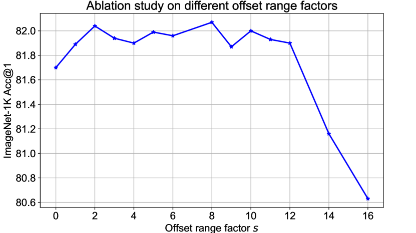
Figure 4: Ablation study on different offset range factor $s$. Accuracies of DAT-T on ImageNet show a wide range of $s$, implying the robustness of this hyper-parameter.

Ablation on different $s$. We go on the further study of the impact of different maximum offsets, i.e., the offset range scale factor $s$ in the paper. We conduct an ablation experiment of $s$ ranging from 0 to 16 where 14 corresponds to the largest reasonable offset given the size of the feature map ($14\times{}14$ at stage 3). As shown in Figure 4, the wide selection range of $s$ shows the robustness of DAT to this hyper-parameter. Practically, we choose a small $s\!=\!2$ for all models in the paper without additional tuning.

4.5 Visualization

To verify the effectiveness of deformable attention, we use a similar mechanism to DCNs to visualize the most important keys across multiple deformable attention layers by propagating their attention weights. As shown in Figure 5, our deformable attention learns to place the keys mostly in the foreground, indicating that it focuses on the important regions of the objects, which supports our hypothesis shown in Figure 1 of the paper. More visualizations can be found in appendix (Figure 6,7).

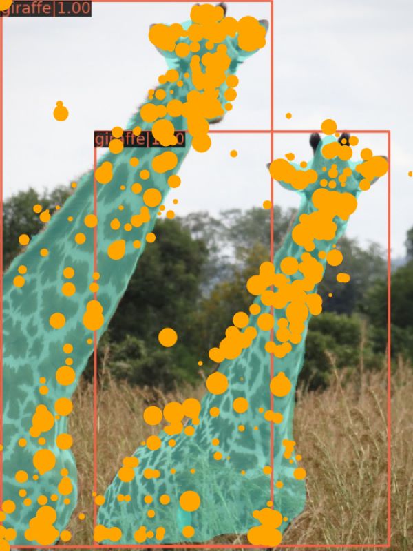
(a)

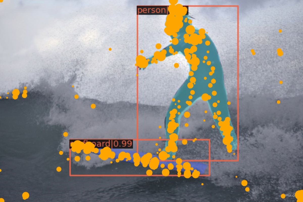
(b)

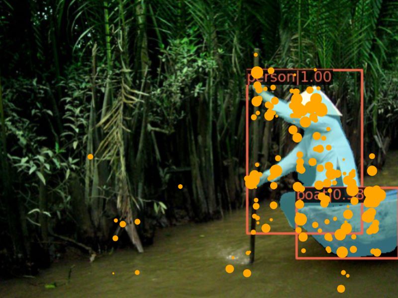
(c)

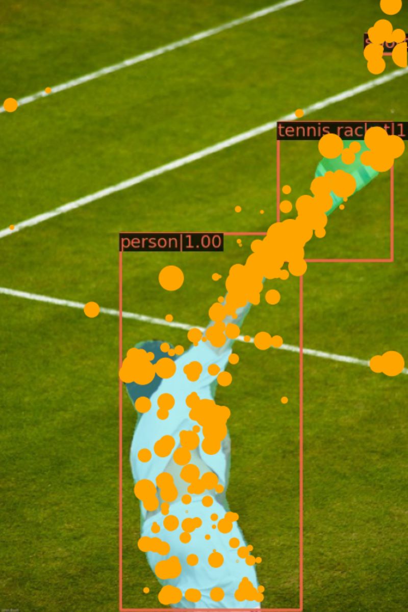
(d)

Figure 5: Visualizations of the most important keys on COCO [25] validation set. The orange circles show the key points with highest propagated attention scores at multiple heads. Larger radius indicate higher score. Note that the bottom right image displays a person waving a racket to hit a tennis ball.

5 Conclusion

This paper presents Deformable Attention Transformer, a novel hierarchical Vision Transformer that can be adapted to both image classification and dense prediction tasks. With deformable attention module, our model is capable of learning sparse-attention patterns in a data-dependent way and modeling geometric transformations. Extensive experiments demonstrate the effectiveness of our model over competitive baselines. We hope our work can inspire insights towards designing flexible attention techniques.

Appendix

A. DAT and Deformable DETR

In this section, we provide a detailed comparision between our proposed deformable attention and the direct adaptation from the deformable convolution [9], which is also known as the multiscale deformable attention in Deformable DETR [54].

First, our deformable attention serves as a feature extractor in the vision backbones while the one in Deformable DETR which replaces the vanilla attention in DETR [4] with a linear deformable attention, plays the role of the detection head. Second, the $m$-th head of query $q$ in the attention in Deformable DETR with single scale is formulated as

$$z^{(m)}_{q}\!=\!\sum_{k=1}^{K}A^{(m)}_{qk}W_{v}\phi(x;p_{q}+\Delta{}p^{(m)}_{qk}),$$ (11)

where $K$ key points are sampled from the input features, mapped by $W_{v}$ and then aggregated by attention weights $A^{(m)}_{qk}$. Compared to our deformable attention (Eq.(9) in the paper), this attention weights is learned from $z_{q}$ by a linear projection, i.e. $A^{(m)}_{qk}=\sigma(W_{\text{att}}x)$, where $W_{\text{att}}\!\in\!\mathbb{R}^{C\times{}MK}$ is the weight matrix to predict the weights of each key on each head, after which a softmax function $\sigma$ is applied to the dimension of $K$ keys to normalize the attention score. In fact, the attention weights are predicted directly by queries instead of measuring the similarities between queries and keys. If we change the $\sigma$ function to a sigmoid, this will be a variant of modulated deformable convolution [53], hence this deformable attention is more similar to convolution rather than attention.

Third, the deformable attention in Deformable DETR is not compatible to the dot-product attention for its enormous memory consumption mentioned in Sec.3.2 in the paper. Therefore, the linear predicted attention is used to avoid computing dot products and a smaller number of keys $K=4$ is also adopted to reduce the memory cost.

To experimentally validate our claim, we replace our deformable attention modules in DAT with the modules in [54] to verify that the naive adaptation is inferior for vision backbone. The comparison results are shown in Table 8. Comparing the first and last row, we can see that under smaller memory budget, the number of keys for the deformable DETR model are set as 16 to reduce memory usage, and achieves $1.4\%$ lower performance. By comparing the third and last row, we can see that the D-DETR attention with the same number of keys as DAT consumes 2.6$\!\times\!$ memory and 1.3$\!\times\!$ FLOPs, while the performances are still lower than DAT.

Attn	Stage 3	Stage 4	FLOPs	#Param	Memory	IN-1K
	#Key	#Key				Acc.
D-DETR	16	16	4.44G	27.95M	13.9GB	80.6
D-DETR	49	49	4.83G	31.15M	18.8GB	80.7
D-DETR	196	49	6.16G	37.26M	37.9GB	79.2
DAT	49	49	4.38G	28.32M	12.5GB	81.8
DAT	196	49	4.59G	28.32M	14.4GB	82.0

Table 8: Comparisons of the deformable attention in DAT with that in [54] under different compuational budgets. The GPU memory cost is measured in a forward pass with a batch size of 64.

B. Adding Convolutions to DAT

Recent works [35, 11, 6, 39] have proved that adopting convolution layers in the Vision Transformer architecture can further improve model performances. For example, using convolutional patch embedding can generally boost model performances by $0.5\%\sim 1.0\%$ on ImageNet classification tasks. It is worth noticing that our proposed DAT can readily combine with these techniques, while we maintain the convolution-free architecture in the main paper to perform fair comparison with baselines.

To fully explore the capacity of DAT, we substitute the patch embedding layers in the original model with strided and overlapped convolutions. The comparison results are shown in Table 9, where baseline models have similar modifications. It is shown that our model with additional convolution modules achieve $0.7\%$ improvement comparing to the original version, and consistently outperform other baselines.

ImageNet-1K Classification
Method	FLOPs	#Param	Top-1 Acc.
CvT-13 [39]	4.5G	20M	81.6
CoAt-Lite Small [42]	4.0G	20M	81.9
CeiT-S [44]	4.8G	24M	82.0
PVTv2-B2 [35]	4.0G	25M	82.0
CoAt Small [42]	12.6G	22M	82.1
RegionViT-S [6]	5.3G	31M	82.5
DAT-T	4.6G	28M	82.0
DAT-T*	4.8G	30M	82.7

Table 9: Comparisons of DAT with other vision transformer backbones on FLOPS, parameters, accuracy on the ImageNet-1K classification task. DAT-T refers to the original version. DAT-T* refers to the model with convolutional patch embeddings.

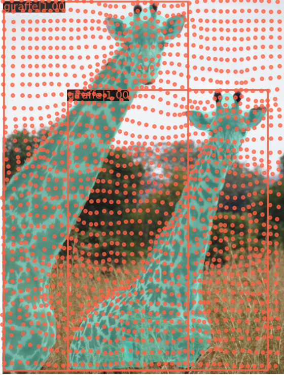
(a)

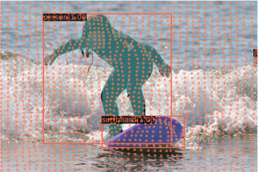
(b)

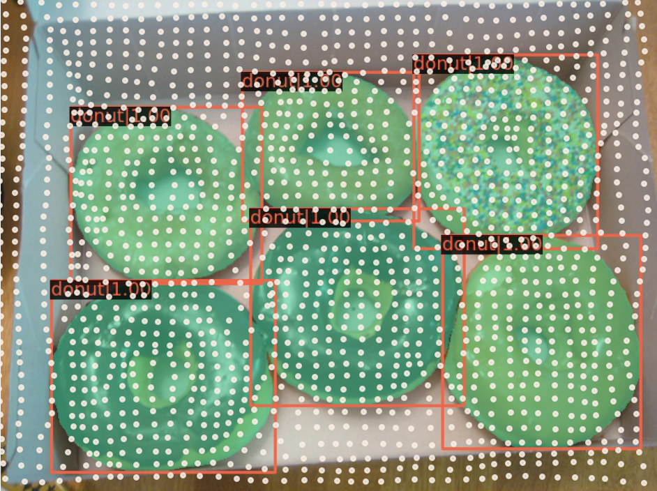
(c)

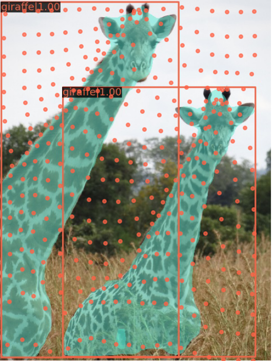
(d)

(e)

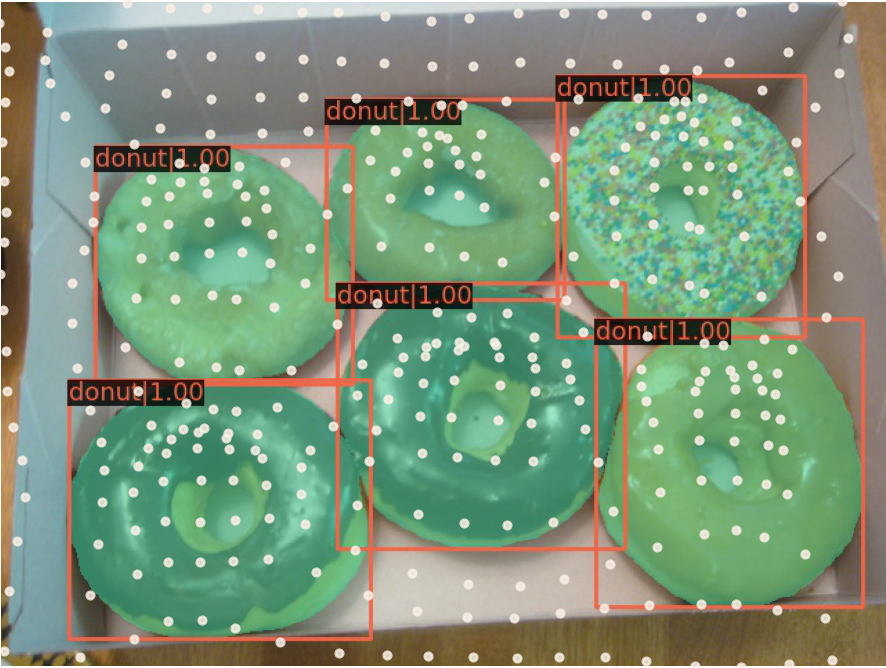
(f)

Figure 6: Visualizations on COCO [25] of learned sampling locations in deformable attention at Stage 3 (first row) and Stage 4 (second row) of DAT. The orange and yellow points show one group of deformed points. The detection bounding boxes and segmentation masks are also presented to indicate the targets.

(a)

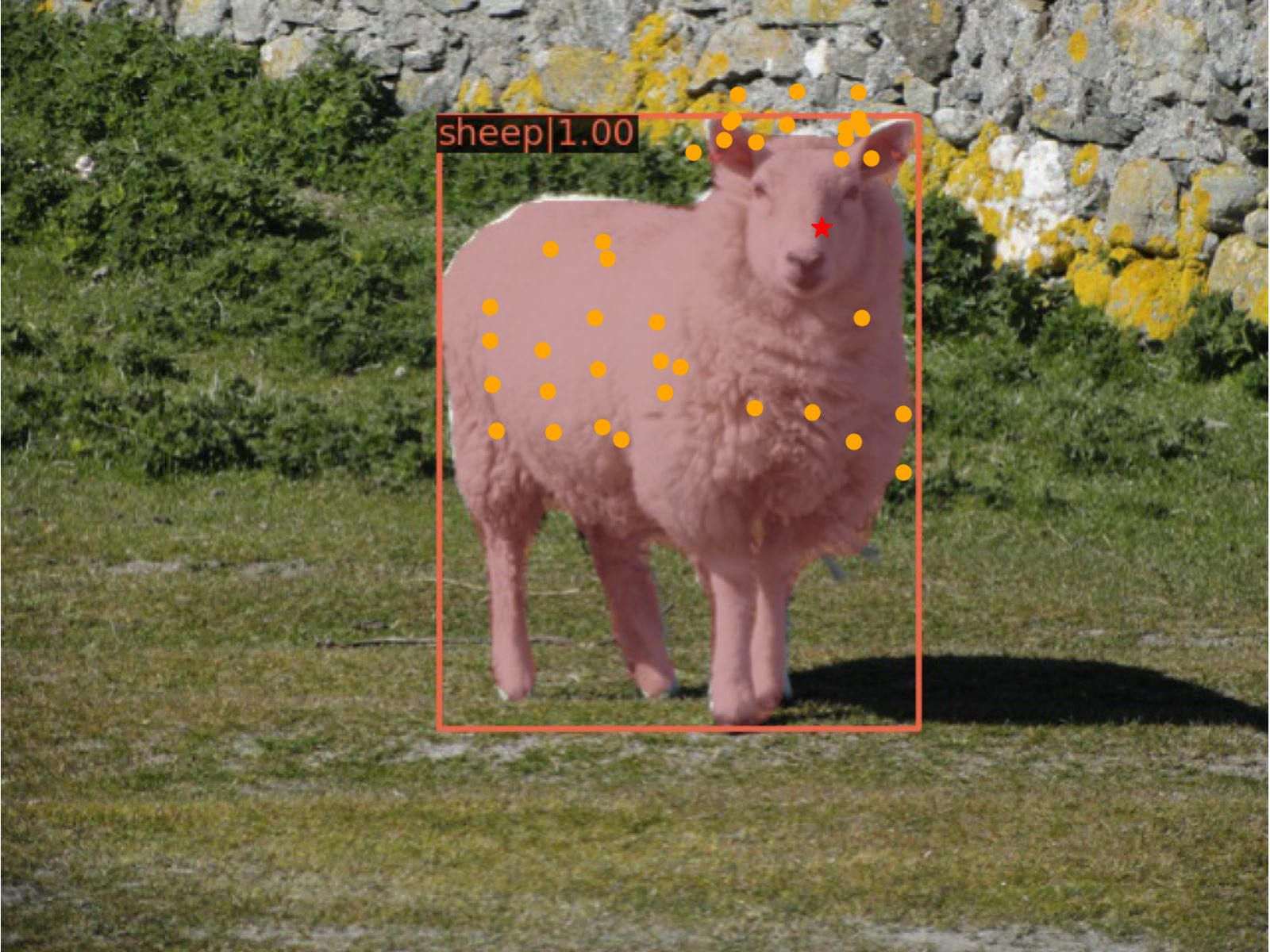
(b)

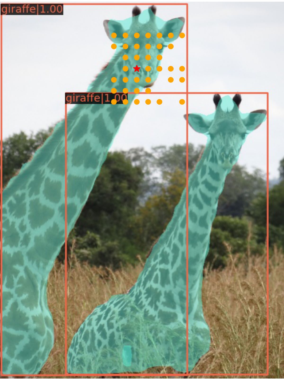
(c)

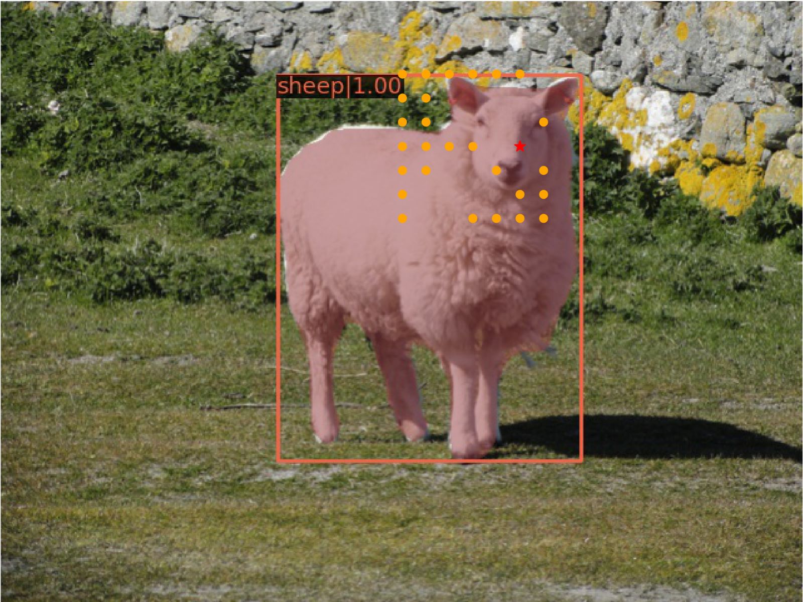
(d)

(e)

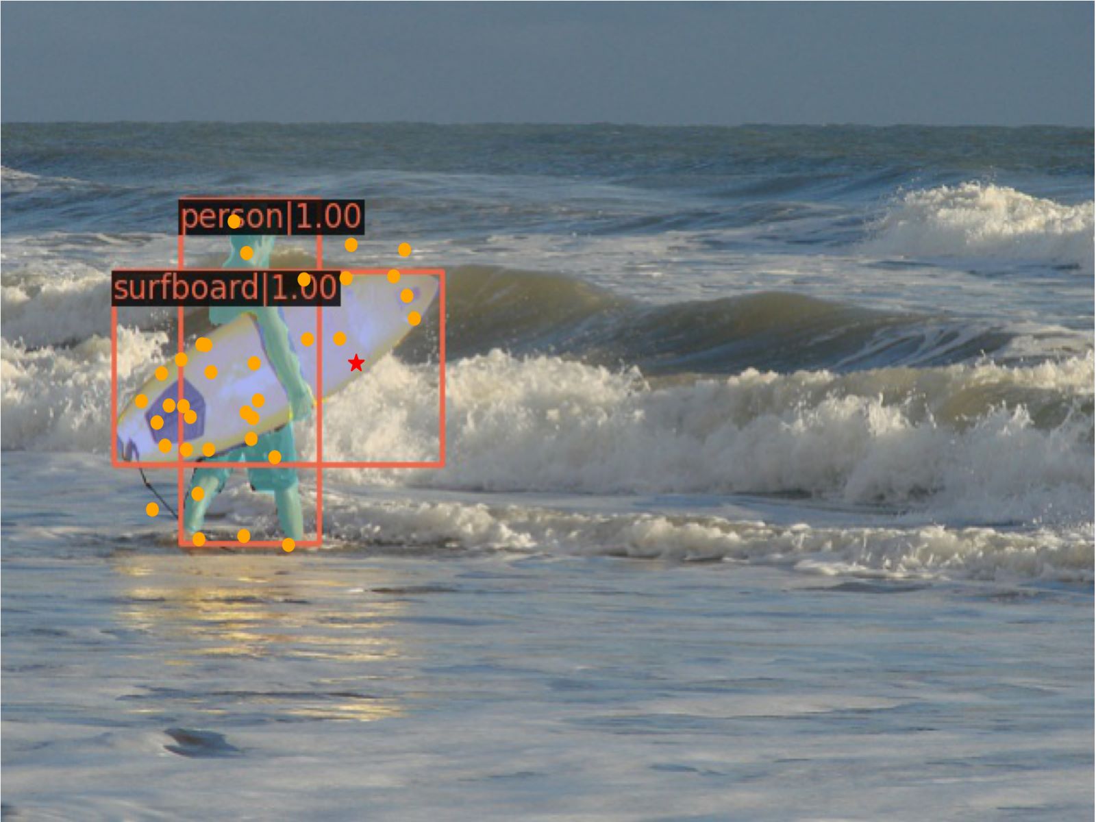
(f)

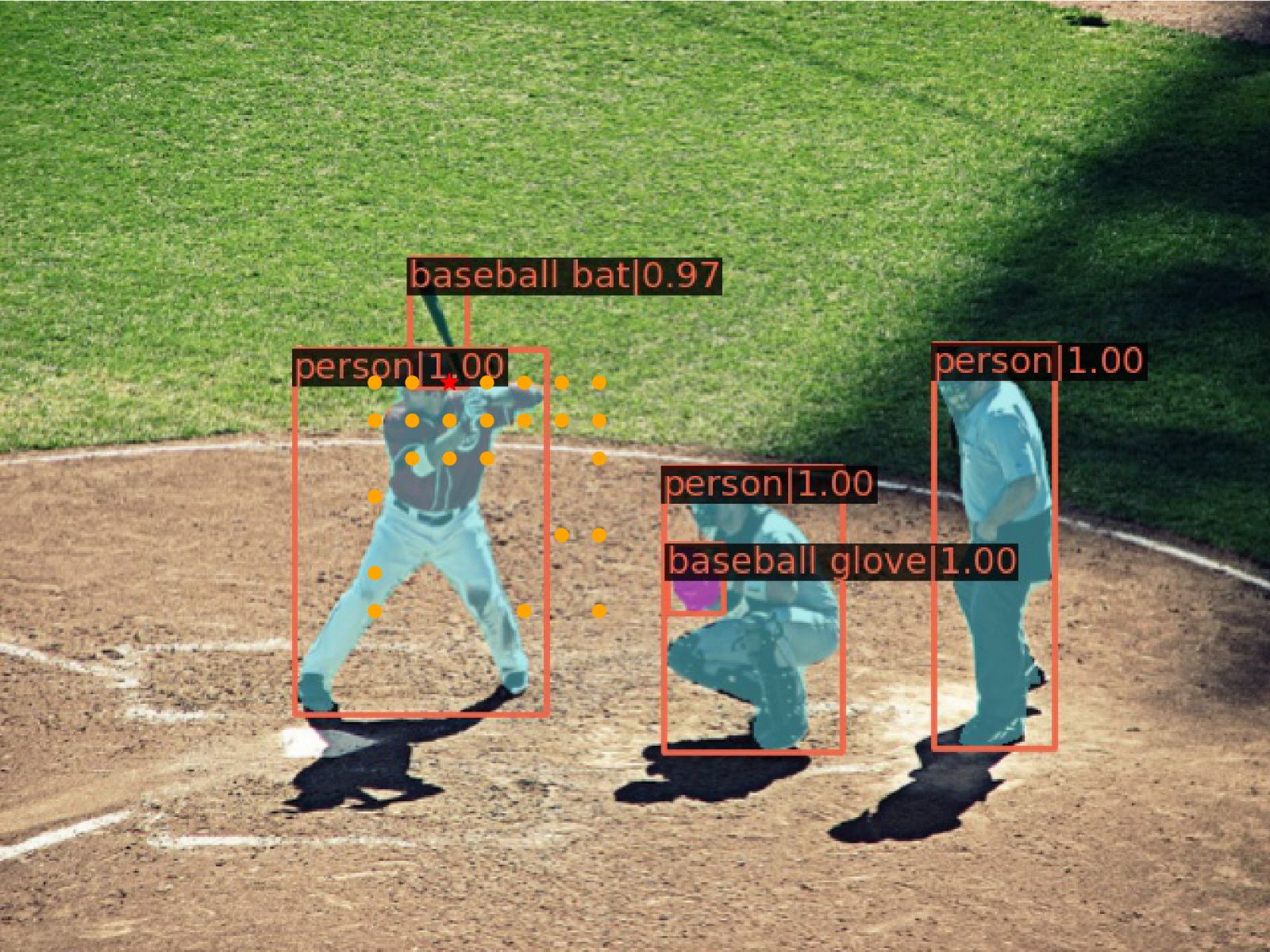
(g)

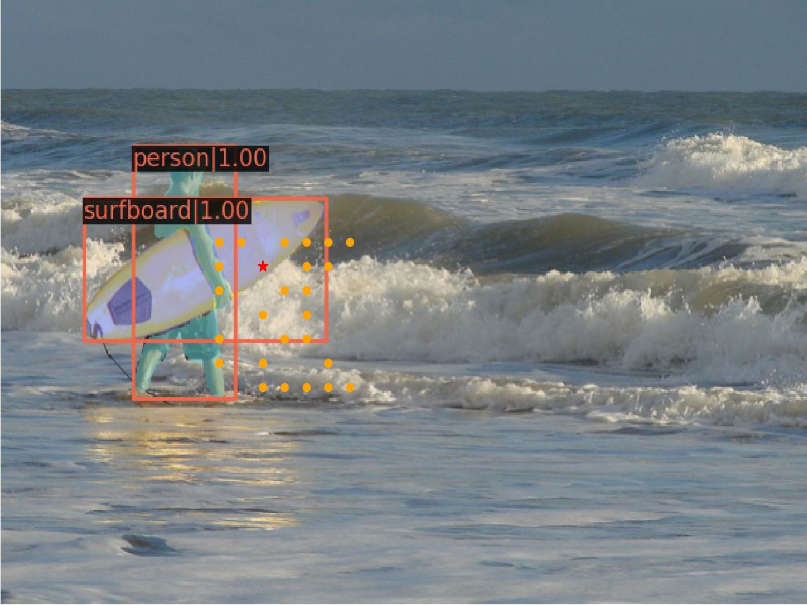
(h)

Figure 7: Visualizations on COCO [25] validation set. The red star denotes a query point, the orange dots are the keys with higher attention scores in the last layer. The images in the first and third rows depict our DAT attention and Swin Transformers’ [26] are shown in the second and fourth rows. The detection bounding boxes and segmentation masks are also presented to indicate the targets.

C. More Visualizations

We visualize examples of learned deformed locations in our DAT to verify the effectiveness of our method. As illustrated in Figure 6, the sampling points are depicted on the top of the object detection boxes and instance segmentation masks, from which we can see that the points are shifted to the target objects. In the left column, the deformed points are contracted to two target giraffes, while other points are keeping a nearly uniform grid with small offsets. In the middle column, the deformed points distribute densely among the person’s body and the surfing board both in the two stages. The right column shows the deformed points focus well to each of the six donuts, which shows our model has the ability to better model geometric shapes even with multiple targets. The above visualizations demonstrate that DAT learns meaningful offsets to sample better keys for attention to improve the performances on various vision tasks.

We also provide visualization results of the attention map given specific query tokens, and compare with Swin Transformer [26] in Figure 7. We show key tokens with the highest attention values. It can be observed that our model focus on the more relevent part. As a showcase, our model allocates most attention to foreground objects, e.g., both gireffas in the first row. On the other hand, the region of interests in Swin Transformer is comparably local and fail to distinguish foreground from background, which is depicted in the last surfboard.

References

- [1] Jimmy Lei Ba, Jamie Ryan Kiros, and Geoffrey E Hinton. Layer normalization. arXiv preprint arXiv:1607.06450, 2016.
- [2] Zhaowei Cai and Nuno Vasconcelos. Cascade r-cnn: Delving into high quality object detection. In CVPR, pages 6154–6162, 2018.
- [3] Yue Cao, Jiarui Xu, Stephen Lin, Fangyun Wei, and Han Hu. Gcnet: Non-local networks meet squeeze-excitation networks and beyond. In ICCVW, pages 0–0, 2019.
- [4] Nicolas Carion, Francisco Massa, Gabriel Synnaeve, Nicolas Usunier, Alexander Kirillov, and Sergey Zagoruyko. End-to-end object detection with transformers. In ECCV, pages 213–229. Springer, 2020.
- [5] Boyu Chen, Peixia Li, Chuming Li, Baopu Li, Lei Bai, Chen Lin, Ming Sun, Junjie Yan, and Wanli Ouyang. Glit: Neural architecture search for global and local image transformer. In ICCV, pages 12–21, October 2021.
- [6] Chun-Fu Chen, Rameswar Panda, and Quanfu Fan. Regionvit: Regional-to-local attention for vision transformers. arXiv preprint arXiv:2106.02689, 2021.
- [7] Zhiyang Chen, Yousong Zhu, Chaoyang Zhao, Guosheng Hu, Wei Zeng, Jinqiao Wang, and Ming Tang. Dpt: Deformable patch-based transformer for visual recognition. In ACM MM, 2021.
- [8] Ekin D Cubuk, Barret Zoph, Jonathon Shlens, and Quoc V Le. Randaugment: Practical automated data augmentation with a reduced search space. In CVPRW, pages 702–703, 2020.
- [9] Jifeng Dai, Haozhi Qi, Yuwen Xiong, Yi Li, Guodong Zhang, Han Hu, and Yichen Wei. Deformable convolutional networks. In ICCV, pages 764–773, 2017.
- [10] Jia Deng, Wei Dong, Richard Socher, Li-Jia Li, Kai Li, and Li Fei-Fei. Imagenet: A large-scale hierarchical image database. In CVPR, pages 248–255. Ieee, 2009.
- [11] Xiaoyi Dong, Jianmin Bao, Dongdong Chen, Weiming Zhang, Nenghai Yu, Lu Yuan, Dong Chen, and Baining Guo. Cswin transformer: A general vision transformer backbone with cross-shaped windows, 2021.
- [12] Alexey Dosovitskiy, Lucas Beyer, Alexander Kolesnikov, Dirk Weissenborn, Xiaohua Zhai, Thomas Unterthiner, Mostafa Dehghani, Matthias Minderer, Georg Heigold, Sylvain Gelly, et al. An image is worth 16x16 words: Transformers for image recognition at scale. In ICLR, 2020.
- [13] Alaaeldin El-Nouby, Hugo Touvron, Mathilde Caron, Piotr Bojanowski, Matthijs Douze, Armand Joulin, Ivan Laptev, Natalia Neverova, Gabriel Synnaeve, Jakob Verbeek, et al. Xcit: Cross-covariance image transformers. arXiv preprint arXiv:2106.09681, 2021.
- [14] Jianyuan Guo, Kai Han, Han Wu, Chang Xu, Yehui Tang, Chunjing Xu, and Yunhe Wang. Cmt: Convolutional neural networks meet vision transformers. arXiv preprint arXiv:2107.06263, 2021.
- [15] Kai Han, An Xiao, Enhua Wu, Jianyuan Guo, Chunjing Xu, and Yunhe Wang. Transformer in transformer. arXiv preprint arXiv:2103.00112, 2021.
- [16] Yizeng Han, Gao Huang, Shiji Song, Le Yang, Yitian Zhang, and Haojun Jiang. Spatially adaptive feature refinement for efficient inference. IEEE TIP, 2021.
- [17] Kaiming He, Georgia Gkioxari, Piotr Dollár, and Ross Girshick. Mask r-cnn. In ICCV, pages 2961–2969, 2017.
- [18] Kaiming He, Xiangyu Zhang, Shaoqing Ren, and Jian Sun. Deep residual learning for image recognition. In CVPR, 2016.
- [19] Gao Huang, Zhuang Liu, Geoff Pleiss, Laurens Van Der Maaten, and Kilian Weinberger. Convolutional networks with dense connectivity. IEEE TPAMI, 2019.
- [20] Gao Huang, Yu Sun, Zhuang Liu, Daniel Sedra, and Kilian Q Weinberger. Deep networks with stochastic depth. In ECCV, pages 646–661. Springer, 2016.
- [21] Andrew Jaegle, Felix Gimeno, Andy Brock, Oriol Vinyals, Andrew Zisserman, and João Carreira. Perceiver: General perception with iterative attention. In ICML, 2021.
- [22] Alexander Kirillov, Ross Girshick, Kaiming He, and Piotr Dollár. Panoptic feature pyramid networks. In CVPR, pages 6399–6408, 2019.
- [23] Tsung-Yi Lin, Piotr Dollár, Ross Girshick, Kaiming He, Bharath Hariharan, and Serge Belongie. Feature pyramid networks for object detection. In CVPR, pages 2117–2125, 2017.
- [24] Tsung-Yi Lin, Priya Goyal, Ross Girshick, Kaiming He, and Piotr Dollár. Focal loss for dense object detection. In ICCV, pages 2980–2988, 2017.
- [25] Tsung-Yi Lin, Michael Maire, Serge Belongie, James Hays, Pietro Perona, Deva Ramanan, Piotr Dollár, and C Lawrence Zitnick. Microsoft coco: Common objects in context. In ECCV, pages 740–755. Springer, 2014.
- [26] Ze Liu, Yutong Lin, Yue Cao, Han Hu, Yixuan Wei, Zheng Zhang, Stephen Lin, and Baining Guo. Swin transformer: Hierarchical vision transformer using shifted windows. ICCV, 2021.
- [27] Ilya Loshchilov and Frank Hutter. Decoupled weight decay regularization. arXiv preprint arXiv:1711.05101, 2017.
- [28] Xuran Pan, Chunjiang Ge, Rui Lu, Shiji Song, Guanfu Chen, Zeyi Huang, and Gao Huang. On the integration of self-attention and convolution, 2021.
- [29] Xuran Pan, Zhuofan Xia, Shiji Song, Li Erran Li, and Gao Huang. 3d object detection with pointformer. In CVPR, 2021.
- [30] Boris T Polyak and Anatoli B Juditsky. Acceleration of stochastic approximation by averaging. SIAM journal on control and optimization, 30(4):838–855, 1992.
- [31] Aravind Srinivas, Tsung-Yi Lin, Niki Parmar, Jonathon Shlens, Pieter Abbeel, and Ashish Vaswani. Bottleneck transformers for visual recognition. In CVPR, pages 16519–16529, 2021.
- [32] Shuyang Sun, Xiaoyu Yue, Song Bai, and Philip H. S. Torr. Visual parser: Representing part-whole hierarchies with transformers.
- [33] Hugo Touvron, Matthieu Cord, Matthijs Douze, Francisco Massa, Alexandre Sablayrolles, and Herve Jegou. Training data-efficient image transformers & distillation through attention. In ICML, volume 139, pages 10347–10357, July 2021.
- [34] Ashish Vaswani, Noam Shazeer, Niki Parmar, Jakob Uszkoreit, Llion Jones, Aidan N Gomez, Łukasz Kaiser, and Illia Polosukhin. Attention is all you need. In NeurIPS, pages 5998–6008, 2017.
- [35] Wenhai Wang, Enze Xie, Xiang Li, Deng-Ping Fan, Kaitao Song, Ding Liang, Tong Lu, Ping Luo, and Ling Shao. Pvtv2: Improved baselines with pyramid vision transformer. arXiv preprint arXiv:2106.13797, 2021.
- [36] Wenhai Wang, Enze Xie, Xiang Li, Deng-Ping Fan, Kaitao Song, Ding Liang, Tong Lu, Ping Luo, and Ling Shao. Pyramid vision transformer: A versatile backbone for dense prediction without convolutions. In ICCV, 2021.
- [37] Yulin Wang, Rui Huang, Shiji Song, Zeyi Huang, and Gao Huang. Not all images are worth 16x16 words: Dynamic transformers for efficient image recognition. NeurIPS, 2021.
- [38] Yulin Wang, Kangchen Lv, Rui Huang, Shiji Song, Le Yang, and Gao Huang. Glance and focus: a dynamic approach to reducing spatial redundancy in image classification. NeurIPS, 2020.
- [39] Haiping Wu, Bin Xiao, Noel Codella, Mengchen Liu, Xiyang Dai, Lu Yuan, and Lei Zhang. Cvt: Introducing convolutions to vision transformers. arXiv preprint arXiv:2103.15808, 2021.
- [40] Tete Xiao, Yingcheng Liu, Bolei Zhou, Yuning Jiang, and Jian Sun. Unified perceptual parsing for scene understanding. In ECCV, pages 418–434, 2018.
- [41] Tete Xiao, Mannat Singh, Eric Mintun, Trevor Darrell, Piotr Dollár, and Ross Girshick. Early convolutions help transformers see better. arXiv preprint arXiv:2106.14881, 2021.
- [42] Weijian Xu, Yifan Xu, Tyler Chang, and Zhuowen Tu. Co-scale conv-attentional image transformers. arXiv preprint arXiv:2104.06399, 2021.
- [43] Jianwei Yang, Chunyuan Li, Pengchuan Zhang, Xiyang Dai, Bin Xiao, Lu Yuan, and Jianfeng Gao. Focal self-attention for local-global interactions in vision transformers. arXiv preprint arXiv:2107.00641, 2021.
- [44] Kun Yuan, Shaopeng Guo, Ziwei Liu, Aojun Zhou, Fengwei Yu, and Wei Wu. Incorporating convolution designs into visual transformers. arXiv preprint arXiv:2103.11816, 2021.
- [45] Yuhui Yuan, Rao Fu, Lang Huang, Weihong Lin, Chao Zhang, Xilin Chen, and Jingdong Wang. Hrformer: High-resolution transformer for dense prediction. arXiv preprint arXiv:2110.09408, 2021.
- [46] Xiaoyu Yue, Shuyang Sun, Zhanghui Kuang, Meng Wei, Philip Torr, Wayne Zhang, and Dahua Lin. Vision transformer with progressive sampling. ICCV, 2021.
- [47] Sangdoo Yun, Dongyoon Han, Seong Joon Oh, Sanghyuk Chun, Junsuk Choe, and Youngjoon Yoo. Cutmix: Regularization strategy to train strong classifiers with localizable features. In ICCV, pages 6023–6032, 2019.
- [48] Hongyi Zhang, Moustapha Cisse, Yann N Dauphin, and David Lopez-Paz. mixup: Beyond empirical risk minimization. arXiv preprint arXiv:1710.09412, 2017.
- [49] Pengchuan Zhang, Xiyang Dai, Jianwei Yang, Bin Xiao, Lu Yuan, Lei Zhang, and Jianfeng Gao. Multi-scale vision longformer: A new vision transformer for high-resolution image encoding. arXiv preprint arXiv:2103.15358, 2021.
- [50] Zhun Zhong, Liang Zheng, Guoliang Kang, Shaozi Li, and Yi Yang. Random erasing data augmentation. In AAAI, volume 34, pages 13001–13008, 2020.
- [51] Bolei Zhou, Hang Zhao, Xavier Puig, Tete Xiao, Sanja Fidler, Adela Barriuso, and Antonio Torralba. Semantic understanding of scenes through the ade20k dataset. IJCV, 127(3):302–321, 2019.
- [52] Daquan Zhou, Bingyi Kang, Xiaojie Jin, Linjie Yang, Xiaochen Lian, Zihang Jiang, Qibin Hou, and Jiashi Feng. Deepvit: Towards deeper vision transformer. arXiv preprint arXiv:2103.11886, 2021.
- [53] Xizhou Zhu, Han Hu, Stephen Lin, and Jifeng Dai. Deformable convnets v2: More deformable, better results. In CVPR, pages 9308–9316, 2019.
- [54] Xizhou Zhu, Weijie Su, Lewei Lu, Bin Li, Xiaogang Wang, and Jifeng Dai. Deformable detr: Deformable transformers for end-to-end object detection. arXiv preprint arXiv:2010.04159, 2020.