Abstract
The minimal supersymmetric extension of the standard model (MSSM) is extended to the U ( 1 ) X 𝑈 subscript 1 𝑋 U(1)_{X} S U ( 3 ) C × S U ( 2 ) L × U ( 1 ) Y × U ( 1 ) X 𝑆 𝑈 subscript 3 𝐶 𝑆 𝑈 subscript 2 𝐿 𝑈 subscript 1 𝑌 𝑈 subscript 1 𝑋 SU(3)_{C}\times SU(2)_{L}\times U(1)_{Y}\times U(1)_{X} U ( 1 ) X 𝑈 subscript 1 𝑋 U(1)_{X} η ^ , η ¯ ^ , S ^ ^ 𝜂 ^ ¯ 𝜂 ^ 𝑆
\hat{\eta},~{}\hat{\bar{\eta}},~{}\hat{S} ν ^ i subscript ^ 𝜈 𝑖 \hat{\nu}_{i} U ( 1 ) X 𝑈 subscript 1 𝑋 U(1)_{X} U ( 1 ) X 𝑈 subscript 1 𝑋 U(1)_{X} ( θ S , θ B B ′ , θ B L ) subscript 𝜃 𝑆 subscript 𝜃 𝐵 superscript 𝐵 ′ subscript 𝜃 𝐵 𝐿 (\theta_{S},\theta_{BB^{\prime}},\theta_{BL})
I Introduction
In 1964, Cronin and Fitch discovered the charge conjugate and parity (CP) violating by the decays of the K 𝐾 K 1964 2 | d e e x p | subscript superscript 𝑑 𝑒 𝑥 𝑝 𝑒 |d^{exp}_{e}| < < 1.1 × 10 − 29 1.1 superscript 10 29 1.1\times 10^{-29} 90 % percent 90 90\% de ; de1 ; de2 | d μ e x p | subscript superscript 𝑑 𝑒 𝑥 𝑝 𝜇 |d^{exp}_{\mu}| < < 1.8 × 10 − 19 1.8 superscript 10 19 1.8\times 10^{-19} 95 % percent 95 95\% | d τ e x p | subscript superscript 𝑑 𝑒 𝑥 𝑝 𝜏 |d^{exp}_{\tau}| < < 1.1 × 10 − 17 1.1 superscript 10 17 1.1\times 10^{-17} 95 % percent 95 95\% pdg NPdl1 ; NPdl2 ; NPdl3 ; NPdl4 mssm ; mssm1 ; mssm2 ; Z2015
Due to the deficiency of MSSM which can not explain neutrino mass and not solve μ 𝜇 \mu U ( 1 ) X 𝑈 subscript 1 𝑋 U(1)_{X} U ( 1 ) Y 𝑈 subscript 1 𝑌 U(1)_{Y} U ( 1 ) X 𝑈 subscript 1 𝑋 U(1)_{X} U ( 1 ) X 𝑈 subscript 1 𝑋 U(1)_{X} extend1 ; extend2 ; extend3 U ( 1 ) X 𝑈 subscript 1 𝑋 U(1)_{X} m h 0 subscript 𝑚 subscript ℎ 0 m_{h_{0}} LCTHiggs1 ; LCTHiggs2 U ( 1 ) X 𝑈 subscript 1 𝑋 U(1)_{X} U ( 1 ) X 𝑈 subscript 1 𝑋 U(1)_{X} m h 0 subscript 𝑚 subscript ℎ 0 m_{h_{0}}
It is an effective way to explore new physics beyond the standard model(SM) that research the MDMs mdms ; mdms1 edms1 ; edms2 ; edms3 ; edms4 ; edms6 ; edms7 ; edms8 d e subscript 𝑑 𝑒 d_{e} mi ; mi1 d e subscript 𝑑 𝑒 d_{e}
In the following, we introduce the specific form of U ( 1 ) X 𝑈 subscript 1 𝑋 U(1)_{X} U ( 1 ) X 𝑈 subscript 1 𝑋 U(1)_{X}
II the U ( 1 ) X 𝑈 subscript 1 𝑋 U(1)_{X}
The U ( 1 ) X 𝑈 subscript 1 𝑋 U(1)_{X} U ( 1 ) X 𝑈 subscript 1 𝑋 U(1)_{X} η ^ , η ¯ ^ , S ^ ^ 𝜂 ^ ¯ 𝜂 ^ 𝑆
\hat{\eta},~{}\hat{\bar{\eta}},~{}\hat{S} ν ^ i subscript ^ 𝜈 𝑖 \hat{\nu}_{i} pro
The superpotential of U ( 1 ) X 𝑈 subscript 1 𝑋 U(1)_{X}
W = l W S ^ + μ H ^ u H ^ d + M S S ^ S ^ − Y d d ^ q ^ H ^ d − Y e e ^ l ^ H ^ d + λ H S ^ H ^ u H ^ d 𝑊 subscript 𝑙 𝑊 ^ 𝑆 𝜇 subscript ^ 𝐻 𝑢 subscript ^ 𝐻 𝑑 subscript 𝑀 𝑆 ^ 𝑆 ^ 𝑆 subscript 𝑌 𝑑 ^ 𝑑 ^ 𝑞 subscript ^ 𝐻 𝑑 subscript 𝑌 𝑒 ^ 𝑒 ^ 𝑙 subscript ^ 𝐻 𝑑 subscript 𝜆 𝐻 ^ 𝑆 subscript ^ 𝐻 𝑢 subscript ^ 𝐻 𝑑 \displaystyle W=l_{W}\hat{S}+\mu\hat{H}_{u}\hat{H}_{d}+M_{S}\hat{S}\hat{S}-Y_{d}\hat{d}\hat{q}\hat{H}_{d}-Y_{e}\hat{e}\hat{l}\hat{H}_{d}+\lambda_{H}\hat{S}\hat{H}_{u}\hat{H}_{d}
+ λ C S ^ η ^ η ¯ ^ + κ 3 S ^ S ^ S ^ + Y u u ^ q ^ H ^ u + Y X ν ^ η ¯ ^ ν ^ + Y ν ν ^ l ^ H ^ u . subscript 𝜆 𝐶 ^ 𝑆 ^ 𝜂 ^ ¯ 𝜂 𝜅 3 ^ 𝑆 ^ 𝑆 ^ 𝑆 subscript 𝑌 𝑢 ^ 𝑢 ^ 𝑞 subscript ^ 𝐻 𝑢 subscript 𝑌 𝑋 ^ 𝜈 ^ ¯ 𝜂 ^ 𝜈 subscript 𝑌 𝜈 ^ 𝜈 ^ 𝑙 subscript ^ 𝐻 𝑢 \displaystyle+\lambda_{C}\hat{S}\hat{\eta}\hat{\bar{\eta}}+\frac{\kappa}{3}\hat{S}\hat{S}\hat{S}+Y_{u}\hat{u}\hat{q}\hat{H}_{u}+Y_{X}\hat{\nu}\hat{\bar{\eta}}\hat{\nu}+Y_{\nu}\hat{\nu}\hat{l}\hat{H}_{u}\;. (1)
These two Higgs doublets and three Higgs singlets are shown below in concrete form,
H u = ( H u + 1 2 ( v u + H u 0 + i P u 0 ) ) , H d = ( 1 2 ( v d + H d 0 + i P d 0 ) H d − ) , formulae-sequence subscript 𝐻 𝑢 superscript subscript 𝐻 𝑢 1 2 subscript 𝑣 𝑢 superscript subscript 𝐻 𝑢 0 𝑖 superscript subscript 𝑃 𝑢 0 subscript 𝐻 𝑑 1 2 subscript 𝑣 𝑑 superscript subscript 𝐻 𝑑 0 𝑖 superscript subscript 𝑃 𝑑 0 superscript subscript 𝐻 𝑑 \displaystyle H_{u}=\left(\begin{array}[]{c}H_{u}^{+}\\
{1\over\sqrt{2}}\Big{(}v_{u}+H_{u}^{0}+iP_{u}^{0}\Big{)}\end{array}\right)\;,~{}~{}~{}~{}~{}~{}H_{d}=\left(\begin{array}[]{c}{1\over\sqrt{2}}\Big{(}v_{d}+H_{d}^{0}+iP_{d}^{0}\Big{)}\\
H_{d}^{-}\end{array}\right)\;, (6)
η = 1 2 ( v η + ϕ η 0 + i P η 0 ) , η ¯ = 1 2 ( v η ¯ + ϕ η ¯ 0 + i P η ¯ 0 ) , formulae-sequence 𝜂 1 2 subscript 𝑣 𝜂 superscript subscript italic-ϕ 𝜂 0 𝑖 superscript subscript 𝑃 𝜂 0 ¯ 𝜂 1 2 subscript 𝑣 ¯ 𝜂 superscript subscript italic-ϕ ¯ 𝜂 0 𝑖 superscript subscript 𝑃 ¯ 𝜂 0 \displaystyle\eta={1\over\sqrt{2}}\Big{(}v_{\eta}+\phi_{\eta}^{0}+iP_{\eta}^{0}\Big{)}\;,~{}~{}~{}~{}~{}~{}~{}~{}~{}~{}~{}~{}~{}~{}~{}\bar{\eta}={1\over\sqrt{2}}\Big{(}v_{\bar{\eta}}+\phi_{\bar{\eta}}^{0}+iP_{\bar{\eta}}^{0}\Big{)}\;,
S = 1 2 ( v S + ϕ S 0 + i P S 0 ) . 𝑆 1 2 subscript 𝑣 𝑆 superscript subscript italic-ϕ 𝑆 0 𝑖 superscript subscript 𝑃 𝑆 0 \displaystyle\hskip 113.81102ptS={1\over\sqrt{2}}\Big{(}v_{S}+\phi_{S}^{0}+iP_{S}^{0}\Big{)}\;. (7)
v u , v d , v η subscript 𝑣 𝑢 subscript 𝑣 𝑑 subscript 𝑣 𝜂
v_{u},~{}v_{d},~{}v_{\eta} v η ¯ subscript 𝑣 ¯ 𝜂 v_{\bar{\eta}} v S subscript 𝑣 𝑆 v_{S} H u subscript 𝐻 𝑢 H_{u} H d subscript 𝐻 𝑑 H_{d} η 𝜂 \eta η ¯ ¯ 𝜂 \bar{\eta} S 𝑆 S
Here, we set tan β = v u / v d 𝛽 subscript 𝑣 𝑢 subscript 𝑣 𝑑 \tan\beta=v_{u}/v_{d} tan β η = v η ¯ / v η subscript 𝛽 𝜂 subscript 𝑣 ¯ 𝜂 subscript 𝑣 𝜂 \tan\beta_{\eta}=v_{\bar{\eta}}/v_{\eta} ν ~ L subscript ~ 𝜈 𝐿 \tilde{\nu}_{L} ν ~ R subscript ~ 𝜈 𝑅 \tilde{\nu}_{R}
ν ~ L = 1 2 ϕ l + i 2 σ l , ν ~ R = 1 2 ϕ R + i 2 σ R . formulae-sequence subscript ~ 𝜈 𝐿 1 2 subscript italic-ϕ 𝑙 𝑖 2 subscript 𝜎 𝑙 subscript ~ 𝜈 𝑅 1 2 subscript italic-ϕ 𝑅 𝑖 2 subscript 𝜎 𝑅 \displaystyle\tilde{\nu}_{L}=\frac{1}{\sqrt{2}}\phi_{l}+\frac{i}{\sqrt{2}}\sigma_{l}\;,~{}~{}~{}~{}~{}~{}~{}~{}~{}~{}\tilde{\nu}_{R}=\frac{1}{\sqrt{2}}\phi_{R}+\frac{i}{\sqrt{2}}\sigma_{R}\;. (8)
The specific form of soft SUSY breaking terms are shown below
ℒ s o f t = ℒ s o f t M S S M − B S S 2 − L S S − T κ 3 S 3 − T λ C S η η ¯ + ϵ i j T λ H S H d i H u j subscript ℒ 𝑠 𝑜 𝑓 𝑡 superscript subscript ℒ 𝑠 𝑜 𝑓 𝑡 𝑀 𝑆 𝑆 𝑀 subscript 𝐵 𝑆 superscript 𝑆 2 subscript 𝐿 𝑆 𝑆 subscript 𝑇 𝜅 3 superscript 𝑆 3 subscript 𝑇 subscript 𝜆 𝐶 𝑆 𝜂 ¯ 𝜂 subscript italic-ϵ 𝑖 𝑗 subscript 𝑇 subscript 𝜆 𝐻 𝑆 superscript subscript 𝐻 𝑑 𝑖 superscript subscript 𝐻 𝑢 𝑗 \displaystyle\mathcal{L}_{soft}=\mathcal{L}_{soft}^{MSSM}-B_{S}S^{2}-L_{S}S-\frac{T_{\kappa}}{3}S^{3}-T_{\lambda_{C}}S\eta\bar{\eta}+\epsilon_{ij}T_{\lambda_{H}}SH_{d}^{i}H_{u}^{j}
− T X I J η ¯ ν ~ R ∗ I ν ~ R ∗ J + ϵ i j T ν I J H u i ν ~ R I ∗ l ~ j J − m η 2 | η | 2 − m η ¯ 2 | η ¯ | 2 superscript subscript 𝑇 𝑋 𝐼 𝐽 ¯ 𝜂 superscript subscript ~ 𝜈 𝑅 absent 𝐼 superscript subscript ~ 𝜈 𝑅 absent 𝐽 subscript italic-ϵ 𝑖 𝑗 subscript superscript 𝑇 𝐼 𝐽 𝜈 superscript subscript 𝐻 𝑢 𝑖 superscript subscript ~ 𝜈 𝑅 𝐼
superscript subscript ~ 𝑙 𝑗 𝐽 superscript subscript 𝑚 𝜂 2 superscript 𝜂 2 superscript subscript 𝑚 ¯ 𝜂 2 superscript ¯ 𝜂 2 \displaystyle-T_{X}^{IJ}\bar{\eta}\tilde{\nu}_{R}^{*I}\tilde{\nu}_{R}^{*J}+\epsilon_{ij}T^{IJ}_{\nu}H_{u}^{i}\tilde{\nu}_{R}^{I*}\tilde{l}_{j}^{J}-m_{\eta}^{2}|\eta|^{2}-m_{\bar{\eta}}^{2}|\bar{\eta}|^{2}
− m S 2 S 2 − ( m ν ~ R 2 ) I J ν ~ R I ∗ ν ~ R J − 1 2 ( M S λ X ~ 2 + 2 M B B ′ λ B ~ λ X ~ ) + h . c . . formulae-sequence superscript subscript 𝑚 𝑆 2 superscript 𝑆 2 superscript superscript subscript 𝑚 subscript ~ 𝜈 𝑅 2 𝐼 𝐽 superscript subscript ~ 𝜈 𝑅 𝐼
superscript subscript ~ 𝜈 𝑅 𝐽 1 2 subscript 𝑀 𝑆 subscript superscript 𝜆 2 ~ 𝑋 2 subscript 𝑀 𝐵 superscript 𝐵 ′ subscript 𝜆 ~ 𝐵 subscript 𝜆 ~ 𝑋 ℎ 𝑐 \displaystyle-m_{S}^{2}S^{2}-(m_{\tilde{\nu}_{R}}^{2})^{IJ}\tilde{\nu}_{R}^{I*}\tilde{\nu}_{R}^{J}-\frac{1}{2}\Big{(}M_{S}\lambda^{2}_{\tilde{X}}+2M_{BB^{\prime}}\lambda_{\tilde{B}}\lambda_{\tilde{X}}\Big{)}+h.c.\;. (9)
The particle content and charge assignments for U ( 1 ) X 𝑈 subscript 1 𝑋 U(1)_{X} 1 U ( 1 ) X 𝑈 subscript 1 𝑋 U(1)_{X} text pro U ( 1 ) Y 𝑈 subscript 1 𝑌 U(1)_{Y} U ( 1 ) X 𝑈 subscript 1 𝑋 U(1)_{X} U ( 1 ) X 𝑈 subscript 1 𝑋 U(1)_{X} M G U T subscript 𝑀 𝐺 𝑈 𝑇 M_{GUT}
Table 1: The superfields in U ( 1 ) X 𝑈 subscript 1 𝑋 U(1)_{X}
The general form of the covariant derivative of this model is model1 ; model2 ; model3
D μ = ∂ μ − i ( Y , X ) ( g Y , g Y X ′ g , ′ X Y g X ′ ) ( A μ ′ Y A μ ′ X ) . \displaystyle D_{\mu}=\partial_{\mu}-i\left(\begin{array}[]{cc}Y,&X\end{array}\right)\left(\begin{array}[]{cc}g_{Y},&g{{}^{\prime}}_{{YX}}\\
g{{}^{\prime}}_{{XY}},&g{{}^{\prime}}_{{X}}\end{array}\right)\left(\begin{array}[]{c}A_{\mu}^{\prime Y}\\
A_{\mu}^{\prime X}\end{array}\right)\;. (15)
The A μ ′ Y superscript subscript 𝐴 𝜇 ′ 𝑌
A_{\mu}^{\prime Y} A μ ′ X subscript superscript 𝐴 ′ 𝑋
𝜇 A^{\prime X}_{\mu} U ( 1 ) Y 𝑈 subscript 1 𝑌 U(1)_{Y} U ( 1 ) X 𝑈 subscript 1 𝑋 U(1)_{X} R 𝑅 R model1 ; model3
( g Y , g Y X ′ g , ′ X Y g X ′ ) R T = ( g 1 , g Y X 0 , g X ) . \displaystyle\left(\begin{array}[]{cc}g_{Y},&g{{}^{\prime}}_{{YX}}\\
g{{}^{\prime}}_{{XY}},&g{{}^{\prime}}_{{X}}\end{array}\right)R^{T}=\left(\begin{array}[]{cc}g_{1},&g_{{YX}}\\
0,&g_{{X}}\end{array}\right)\;. (20)
We deduce sin 2 θ W ′ superscript 2 superscript subscript 𝜃 𝑊 ′ \sin^{2}\theta_{W}^{\prime} = =
1 2 − ( ( g Y X + g X ) 2 − g 1 2 − g 2 2 ) v 2 + 4 g X 2 ξ 2 2 ( ( g Y X + g X ) 2 + g 1 2 + g 2 2 ) 2 v 4 + 8 g X 2 ( ( g Y X + g X ) 2 − g 1 2 − g 2 2 ) v 2 ξ 2 + 16 g X 4 ξ 4 . 1 2 superscript subscript 𝑔 𝑌 𝑋 subscript 𝑔 𝑋 2 superscript subscript 𝑔 1 2 superscript subscript 𝑔 2 2 superscript 𝑣 2 4 superscript subscript 𝑔 𝑋 2 superscript 𝜉 2 2 superscript superscript subscript 𝑔 𝑌 𝑋 subscript 𝑔 𝑋 2 superscript subscript 𝑔 1 2 superscript subscript 𝑔 2 2 2 superscript 𝑣 4 8 superscript subscript 𝑔 𝑋 2 superscript subscript 𝑔 𝑌 𝑋 subscript 𝑔 𝑋 2 superscript subscript 𝑔 1 2 superscript subscript 𝑔 2 2 superscript 𝑣 2 superscript 𝜉 2 16 superscript subscript 𝑔 𝑋 4 superscript 𝜉 4 \displaystyle\frac{1}{2}-\frac{((g_{YX}+g_{X})^{2}-g_{1}^{2}-g_{2}^{2})v^{2}+4g_{X}^{2}\xi^{2}}{2\sqrt{((g_{YX}+g_{X})^{2}+g_{1}^{2}+g_{2}^{2})^{2}v^{4}+8g_{X}^{2}((g_{YX}+g_{X})^{2}-g_{1}^{2}-g_{2}^{2})v^{2}\xi^{2}+16g_{X}^{4}\xi^{4}}}\;. (21)
with ξ = v η 2 + v η ¯ 2 𝜉 superscript subscript 𝑣 𝜂 2 superscript subscript 𝑣 ¯ 𝜂 2 \xi=\sqrt{v_{\eta}^{2}+v_{\bar{\eta}}^{2}} θ W ′ superscript subscript 𝜃 𝑊 ′ \theta_{W}^{\prime} Z 𝑍 Z Z ′ superscript 𝑍 ′ Z^{\prime}
Next, we describe some of the couplings needed.
The couplings of ν ~ k R − e ¯ i − χ j − subscript superscript ~ 𝜈 𝑅 𝑘 subscript ¯ 𝑒 𝑖 superscript subscript 𝜒 𝑗 \tilde{\nu}^{R}_{k}-\bar{e}_{i}-\chi_{j}^{-} ν ~ k I − e ¯ i − χ j − subscript superscript ~ 𝜈 𝐼 𝑘 subscript ¯ 𝑒 𝑖 superscript subscript 𝜒 𝑗 \tilde{\nu}^{I}_{k}-\bar{e}_{i}-\chi_{j}^{-}
ℒ ν ~ R e ¯ χ − = e ¯ i { i 2 U j 2 ∗ Z k i R ∗ Y e i P L − i 2 g 2 V j 1 Z k i R ∗ P R } χ j − ν ~ k R , subscript ℒ superscript ~ 𝜈 𝑅 ¯ 𝑒 superscript 𝜒 subscript ¯ 𝑒 𝑖 𝑖 2 subscript superscript 𝑈 𝑗 2 subscript superscript 𝑍 𝑅
𝑘 𝑖 superscript subscript 𝑌 𝑒 𝑖 subscript 𝑃 𝐿 𝑖 2 subscript 𝑔 2 subscript 𝑉 𝑗 1 subscript superscript 𝑍 𝑅
𝑘 𝑖 subscript 𝑃 𝑅 superscript subscript 𝜒 𝑗 subscript superscript ~ 𝜈 𝑅 𝑘 \displaystyle\mathcal{L}_{\tilde{\nu}^{R}\bar{e}\chi^{-}}=\bar{e}_{i}\Big{\{}\frac{i}{\sqrt{2}}U^{*}_{j2}Z^{R*}_{ki}Y_{e}^{i}P_{L}-\frac{i}{\sqrt{2}}g_{2}V_{j1}Z^{R*}_{ki}P_{R}\Big{\}}\chi_{j}^{-}\tilde{\nu}^{R}_{k}\;, (22)
ℒ ν ~ I e ¯ χ − = e ¯ i { − 1 2 U j 2 ∗ Z k i I ∗ Y e i P L + 1 2 g 2 V j 1 Z k i I ∗ P R } χ j − ν ~ k I . subscript ℒ superscript ~ 𝜈 𝐼 ¯ 𝑒 superscript 𝜒 subscript ¯ 𝑒 𝑖 1 2 subscript superscript 𝑈 𝑗 2 subscript superscript 𝑍 𝐼
𝑘 𝑖 superscript subscript 𝑌 𝑒 𝑖 subscript 𝑃 𝐿 1 2 subscript 𝑔 2 subscript 𝑉 𝑗 1 subscript superscript 𝑍 𝐼
𝑘 𝑖 subscript 𝑃 𝑅 superscript subscript 𝜒 𝑗 subscript superscript ~ 𝜈 𝐼 𝑘 \displaystyle\mathcal{L}_{\tilde{\nu}^{I}\bar{e}\chi^{-}}=\bar{e}_{i}\Big{\{}\frac{-1}{\sqrt{2}}U^{*}_{j2}Z^{I*}_{ki}Y_{e}^{i}P_{L}+\frac{1}{\sqrt{2}}g_{2}V_{j1}Z^{I*}_{ki}P_{R}\Big{\}}\chi_{j}^{-}\tilde{\nu}^{I}_{k}\;. (23)
With P L = 1 − γ 5 2 subscript 𝑃 𝐿 1 subscript 𝛾 5 2 P_{L}=\frac{1-\gamma_{5}}{2} P R = 1 + γ 5 2 subscript 𝑃 𝑅 1 subscript 𝛾 5 2 P_{R}=\frac{1+\gamma_{5}}{2} Z R superscript 𝑍 𝑅 Z^{R} Z I superscript 𝑍 𝐼 Z^{I} U 𝑈 U V 𝑉 V
We also deduce the vertex couplings of neutrino-slepton-chargino and neutralino-lepton-slepton,
ℒ ν ¯ χ − L ~ = ν ¯ i ( ( − g 2 U j 1 ∗ ∑ a = 1 3 U i a V ∗ Z k a E + U j 2 ∗ ∑ a = 1 3 U i a V ∗ Y l a Z k ( 3 + a ) E ) P L \displaystyle\mathcal{L}_{\bar{\nu}\chi^{-}\tilde{L}}=\bar{\nu}_{i}\Big{(}(-g_{2}U^{*}_{j1}\sum_{a=1}^{3}U^{V*}_{ia}Z^{E}_{ka}+U^{*}_{j2}\sum_{a=1}^{3}U^{V*}_{ia}Y^{a}_{l}Z^{E}_{k(3+a)})P_{L}
+ ∑ a , b = 1 3 Y ν a b U i ( 3 + a ) V Z k b E V j 2 P R ) χ − j L ~ k , \displaystyle\hskip 45.52458pt+\sum_{a,b=1}^{3}Y_{\nu}^{ab}U^{V}_{i(3+a)}Z^{E}_{kb}V_{j2}P_{R}\Big{)}\chi^{-}_{j}\tilde{L}_{k}\;, (24)
ℒ χ ¯ 0 l L ~ = χ ¯ i 0 { ( 1 2 ( g 1 N i 1 ∗ + g 2 N i 2 ∗ + g Y X N i 5 ∗ ) Z k j E − N i 3 ∗ Y l j Z k ( 3 + j ) E ) P L \displaystyle\mathcal{L}_{\bar{\chi}^{0}l\tilde{L}}=\bar{\chi}^{0}_{i}\Big{\{}\Big{(}\frac{1}{\sqrt{2}}(g_{1}N^{*}_{i1}+g_{2}N^{*}_{i2}+g_{YX}N^{*}_{i5})Z^{E}_{kj}-N^{*}_{i3}Y^{j}_{l}Z^{E}_{k(3+j)}\Big{)}P_{L}
− [ 1 2 ( 2 g 1 N i 1 + ( 2 g Y X + g X ) N i 5 ) Z k ( 3 + a ) E + Y l j Z k j E N i 3 ] P R } l j L ~ k . \displaystyle\hskip 45.52458pt-\Big{[}\frac{1}{\sqrt{2}}\Big{(}2g_{1}N_{i1}+(2g_{YX}+g_{X})N_{i5}\Big{)}Z^{E}_{k(3+a)}+Y_{l}^{j}Z^{E}_{kj}N_{i3}\Big{]}P_{R}\Big{\}}l_{j}\tilde{L}_{k}\;. (25)
With Z E superscript 𝑍 𝐸 Z^{E} N 𝑁 N U V superscript 𝑈 𝑉 U^{V}
Other couplings needed can be found in our previous works pro ; slh
III formulation
The Feynman amplitude can be expressed by these dimension 6 operators lepton m μ 2 M S U S Y 2 superscript subscript 𝑚 𝜇 2 superscript subscript 𝑀 𝑆 𝑈 𝑆 𝑌 2 \frac{m_{\mu}^{2}}{M_{SUSY}^{2}} ∼ similar-to \sim 10 − 7 superscript 10 7 10^{-7} 10 − 8 superscript 10 8 10^{-8}
These dimension 6 operators are shown below
𝒪 1 ∓ = 1 ( 4 π ) 2 l ¯ ( i 𝒟 / ) 3 ω ∓ l , \displaystyle\mathcal{O}_{1}^{\mp}=\frac{1}{(4\pi)^{2}}\bar{l}(i\mathcal{D}\!\!\!/)^{3}\omega_{\mp}l\;,
𝒪 2 ∓ = e Q f ( 4 π ) 2 ( i 𝒟 μ l ) ¯ γ μ F ⋅ σ ω ∓ l , superscript subscript 𝒪 2 minus-or-plus ⋅ 𝑒 subscript 𝑄 𝑓 superscript 4 𝜋 2 ¯ 𝑖 subscript 𝒟 𝜇 𝑙 superscript 𝛾 𝜇 𝐹 𝜎 subscript 𝜔 minus-or-plus 𝑙 \displaystyle\mathcal{O}_{2}^{\mp}=\frac{eQ_{f}}{(4\pi)^{2}}\overline{(i\mathcal{D}_{\mu}l)}\gamma^{\mu}F\cdot\sigma\omega_{\mp}l\;,
𝒪 3 ∓ = e Q f ( 4 π ) 2 l ¯ F ⋅ σ γ μ ω ∓ ( i 𝒟 μ l ) , superscript subscript 𝒪 3 minus-or-plus ⋅ 𝑒 subscript 𝑄 𝑓 superscript 4 𝜋 2 ¯ 𝑙 𝐹 𝜎 superscript 𝛾 𝜇 subscript 𝜔 minus-or-plus 𝑖 subscript 𝒟 𝜇 𝑙 \displaystyle\mathcal{O}_{3}^{\mp}=\frac{eQ_{f}}{(4\pi)^{2}}\bar{l}F\cdot\sigma\gamma^{\mu}\omega_{\mp}(i\mathcal{D}_{\mu}l)\;,
𝒪 4 ∓ = e Q f ( 4 π ) 2 l ¯ ( ∂ μ F μ ν ) γ ν ω ∓ l , superscript subscript 𝒪 4 minus-or-plus 𝑒 subscript 𝑄 𝑓 superscript 4 𝜋 2 ¯ 𝑙 superscript 𝜇 subscript 𝐹 𝜇 𝜈 superscript 𝛾 𝜈 subscript 𝜔 minus-or-plus 𝑙 \displaystyle\mathcal{O}_{4}^{\mp}=\frac{eQ_{f}}{(4\pi)^{2}}\bar{l}(\partial^{\mu}F_{\mu\nu})\gamma^{\nu}\omega_{\mp}l,
𝒪 5 ∓ = m l ( 4 π ) 2 l ¯ ( i 𝒟 / ) 2 ω ∓ l , \displaystyle\mathcal{O}_{5}^{\mp}=\frac{m_{l}}{(4\pi)^{2}}\bar{l}(i\mathcal{D}\!\!\!/)^{2}\omega_{\mp}l\;,
𝒪 6 ∓ = e Q f m l ( 4 π ) 2 l ¯ F ⋅ σ ω ∓ l . superscript subscript 𝒪 6 minus-or-plus ⋅ 𝑒 subscript 𝑄 𝑓 subscript 𝑚 𝑙 superscript 4 𝜋 2 ¯ 𝑙 𝐹 𝜎 subscript 𝜔 minus-or-plus 𝑙 \displaystyle\mathcal{O}_{6}^{\mp}=\frac{eQ_{f}m_{l}}{(4\pi)^{2}}\bar{l}F\cdot\sigma\omega_{\mp}l\;. (26)
Here, 𝒟 μ = ∂ μ + i e A μ subscript 𝒟 𝜇 subscript 𝜇 𝑖 𝑒 subscript 𝐴 𝜇 \mathcal{D}_{\mu}=\partial_{\mu}+ieA_{\mu} ω ∓ = 1 ∓ γ 5 2 subscript 𝜔 minus-or-plus minus-or-plus 1 subscript 𝛾 5 2 \omega_{\mp}=\frac{1\mp\gamma_{5}}{2} F μ ν subscript 𝐹 𝜇 𝜈 F_{{\mu\nu}} m l subscript 𝑚 𝑙 m_{{}_{l}}
The effective Lagrangian of lepton EDM is
ℒ E D M = − i 2 d l l ¯ σ μ ν γ 5 l F μ ν . subscript ℒ 𝐸 𝐷 𝑀 𝑖 2 subscript 𝑑 𝑙 ¯ 𝑙 superscript 𝜎 𝜇 𝜈 subscript 𝛾 5 𝑙 subscript 𝐹 𝜇 𝜈 \displaystyle{\cal L}_{{}_{EDM}}=\frac{-i}{2}d_{l}\bar{l}\sigma^{\mu\nu}\gamma_{5}lF_{\mu\nu}\;. (27)
For Fermions EDM cannot be obtained at tree level in the fundamental interaction because it is a CP violation amplitude. Then, the one-loop diagrams should have non-zero contribution to Fermion EDM in the CP violating electroweak theory. With the relationship between the Wilson coefficients C 2 , 3 , 6 ∓ superscript subscript 𝐶 2 3 6
minus-or-plus C_{2,3,6}^{\mp} 𝒪 2 , 3 , 6 ∓ superscript subscript 𝒪 2 3 6
minus-or-plus \mathcal{O}_{2,3,6}^{\mp} lepton ; edms6 ; edms7 ; edms8
d l = − 2 e Q f m l ( 4 π ) 2 ℑ ( C 2 + + C 2 − ∗ + C 6 + ) . subscript 𝑑 𝑙 2 𝑒 subscript 𝑄 𝑓 subscript 𝑚 𝑙 superscript 4 𝜋 2 superscript subscript 𝐶 2 superscript subscript 𝐶 2 absent superscript subscript 𝐶 6 \displaystyle d_{l}=\frac{-2eQ_{f}m_{l}}{(4\pi)^{2}}\Im(C_{2}^{+}+C_{2}^{-*}+C_{6}^{+})\;. (28)
III.1 The one-loop corrections
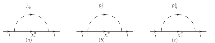
The one-loop new physics contributions to lepton EDMs come from the diagrams in FIG. 1. The one-loop contributions to lepton EDMs are obtained by calculating with the on-shell condition of external lepton. Then we simplify the analytical results.
Figure 1: The one-loop self energy diagrams in the U ( 1 ) X 𝑈 subscript 1 𝑋 U(1)_{X}
The analytical results of the one-loop diagrams are shown below
1. The corrections to lepton EDMs from neutralinos and scalar leptons are
d l L ~ χ 0 = ( − e 2 Λ ) ℑ [ − ∑ i = 1 8 ∑ j = 1 6 { ( A L ∗ A R ) x χ i 0 x L ~ j ∂ 2 ℬ ( x χ i 0 , x L ~ j ) ∂ x L ~ j 2 } ] . superscript subscript 𝑑 𝑙 ~ 𝐿 superscript 𝜒 0 𝑒 2 Λ superscript subscript 𝑖 1 8 superscript subscript 𝑗 1 6 superscript subscript 𝐴 𝐿 subscript 𝐴 𝑅 subscript 𝑥 superscript subscript 𝜒 𝑖 0 subscript 𝑥 subscript ~ 𝐿 𝑗 superscript 2 ℬ subscript 𝑥 superscript subscript 𝜒 𝑖 0 subscript 𝑥 subscript ~ 𝐿 𝑗 superscript subscript 𝑥 subscript ~ 𝐿 𝑗 2 \displaystyle d_{l}^{\tilde{L}\chi^{0}}=(\frac{-e}{2\Lambda})\Im\left[-\sum_{i=1}^{8}\sum_{j=1}^{6}\Big{\{}(A_{L}^{*}A_{R})\sqrt{x_{\chi_{i}^{0}}}x_{\tilde{L}_{j}}\frac{\partial^{2}\mathcal{B}(x_{\chi_{i}^{0}},x_{\tilde{L}_{j}})}{\partial x_{\tilde{L}_{j}}^{2}}\Big{\}}\right]\;. (29)
With x i = m i 2 Λ 2 subscript 𝑥 𝑖 superscript subscript 𝑚 𝑖 2 superscript Λ 2 x_{i}=\frac{m_{i}^{2}}{\Lambda^{2}} m i subscript 𝑚 𝑖 m_{i} Λ Λ \Lambda A R , A L subscript 𝐴 𝑅 subscript 𝐴 𝐿
A_{R},A_{L}
A R = 1 2 g 1 N i 1 ∗ Z j 2 E + 1 2 g 2 N i 2 ∗ Z j 2 E + 1 2 g Y X N i 5 ∗ Z j 2 E − N i 3 ∗ Y μ Z j 5 E , subscript 𝐴 𝑅 1 2 subscript 𝑔 1 superscript subscript 𝑁 𝑖 1 superscript subscript 𝑍 𝑗 2 𝐸 1 2 subscript 𝑔 2 superscript subscript 𝑁 𝑖 2 superscript subscript 𝑍 𝑗 2 𝐸 1 2 subscript 𝑔 𝑌 𝑋 superscript subscript 𝑁 𝑖 5 superscript subscript 𝑍 𝑗 2 𝐸 superscript subscript 𝑁 𝑖 3 subscript 𝑌 𝜇 superscript subscript 𝑍 𝑗 5 𝐸 \displaystyle A_{R}=\frac{1}{\sqrt{2}}g_{1}N_{i1}^{*}Z_{j2}^{E}+\frac{1}{\sqrt{2}}g_{2}N_{i2}^{*}Z_{j2}^{E}+\frac{1}{\sqrt{2}}g_{YX}N_{i5}^{*}Z_{j2}^{E}-N_{i3}^{*}Y_{\mu}Z_{j5}^{E}\;,
A L = − 1 2 Z j 5 E ( 2 g 1 N i 1 + ( 2 g Y X + g X ) N i 5 ) − Y μ ∗ Z j 2 E N i 3 . subscript 𝐴 𝐿 1 2 superscript subscript 𝑍 𝑗 5 𝐸 2 subscript 𝑔 1 subscript 𝑁 𝑖 1 2 subscript 𝑔 𝑌 𝑋 subscript 𝑔 𝑋 subscript 𝑁 𝑖 5 superscript subscript 𝑌 𝜇 superscript subscript 𝑍 𝑗 2 𝐸 subscript 𝑁 𝑖 3 \displaystyle A_{L}=-\frac{1}{\sqrt{2}}Z_{j5}^{E}(2g_{1}N_{i1}+(2g_{YX}+g_{X})N_{i5})-Y_{\mu}^{*}Z_{j2}^{E}N_{i3}\;. (30)
The mass matrices of scalar leptons and neutrinos can be diagonalized using the matrices Z E superscript 𝑍 𝐸 Z^{E} N 𝑁 N
The specific forms of functions ℬ ( x , y ) ℬ 𝑥 𝑦 \mathcal{B}(x,y) ℬ 1 ( x , y ) subscript ℬ 1 𝑥 𝑦 \mathcal{B}_{1}(x,y)
ℬ ( x , y ) = 1 16 π 2 ( x ln x y − x + y ln y x − y ) , ℬ 1 ( x , y ) = ( ∂ ∂ y + y 2 ∂ 2 ∂ y 2 ) ℬ ( x , y ) . formulae-sequence ℬ 𝑥 𝑦 1 16 superscript 𝜋 2 𝑥 𝑥 𝑦 𝑥 𝑦 𝑦 𝑥 𝑦 subscript ℬ 1 𝑥 𝑦 𝑦 𝑦 2 superscript 2 superscript 𝑦 2 ℬ 𝑥 𝑦 \displaystyle\mathcal{B}(x,y)=\frac{1}{16\pi^{2}}\Big{(}\frac{x\ln x}{y-x}+\frac{y\ln y}{x-y}\Big{)}\;,~{}~{}~{}\mathcal{B}_{1}(x,y)=(\frac{\partial}{\partial y}+\frac{y}{2}\frac{\partial^{2}}{\partial y^{2}})\mathcal{B}(x,y)\;. (31)
2. The corrections from chargino and CP-odd scalar neutrino are
d l I ν ~ χ ± = ( − e 2 Λ ) ℑ [ ∑ i = 1 2 ∑ j = 1 6 { − 2 ( B L ∗ B R ) x χ i − ℬ 1 ( x ν ~ j I , x χ i − ) } ] . superscript subscript 𝑑 𝑙 𝐼 ~ 𝜈 superscript 𝜒 plus-or-minus 𝑒 2 Λ superscript subscript 𝑖 1 2 superscript subscript 𝑗 1 6 2 superscript subscript 𝐵 𝐿 subscript 𝐵 𝑅 subscript 𝑥 superscript subscript 𝜒 𝑖 subscript ℬ 1 subscript 𝑥 superscript subscript ~ 𝜈 𝑗 𝐼 subscript 𝑥 superscript subscript 𝜒 𝑖 \displaystyle d_{lI}^{\tilde{\nu}\chi^{\pm}}=(\frac{-e}{2\Lambda})\Im\left[\sum_{i=1}^{2}\sum_{j=1}^{6}\Big{\{}-2(B_{L}^{*}B_{R})\sqrt{x_{\chi_{i}^{-}}}\mathcal{B}_{1}(x_{\tilde{\nu}_{j}^{I}},x_{\chi_{i}^{-}})\Big{\}}\right]\;. (32)
The couplings B L subscript 𝐵 𝐿 B_{L} B R subscript 𝐵 𝑅 B_{R}
B L = − 1 2 U i 2 ∗ Z j 2 I ∗ Y μ , B R = 1 2 g 2 Z j 2 I ∗ V i 1 . formulae-sequence subscript 𝐵 𝐿 1 2 superscript subscript 𝑈 𝑖 2 superscript subscript 𝑍 𝑗 2 𝐼
subscript 𝑌 𝜇 subscript 𝐵 𝑅 1 2 subscript 𝑔 2 superscript subscript 𝑍 𝑗 2 𝐼
subscript 𝑉 𝑖 1 \displaystyle B_{L}=-\frac{1}{\sqrt{2}}U_{i2}^{*}Z_{j2}^{I*}Y_{\mu}\;,~{}~{}~{}B_{R}=\frac{1}{\sqrt{2}}g_{2}Z_{j2}^{I*}V_{i1}\;. (33)
3. The corrections from chargino and CP-even scalar neutrino are
d l R ν ~ χ ± = ( − e 2 Λ ) ℑ [ ∑ i = 1 2 ∑ j = 1 6 { − 2 ( C L ∗ C R ) x χ i − ℬ 1 ( x ν ~ j R , x χ i − ) } ] . superscript subscript 𝑑 𝑙 𝑅 ~ 𝜈 superscript 𝜒 plus-or-minus 𝑒 2 Λ superscript subscript 𝑖 1 2 superscript subscript 𝑗 1 6 2 superscript subscript 𝐶 𝐿 subscript 𝐶 𝑅 subscript 𝑥 superscript subscript 𝜒 𝑖 subscript ℬ 1 subscript 𝑥 superscript subscript ~ 𝜈 𝑗 𝑅 subscript 𝑥 superscript subscript 𝜒 𝑖 \displaystyle d_{lR}^{\tilde{\nu}\chi^{\pm}}=(\frac{-e}{2\Lambda})\Im\left[\sum_{i=1}^{2}\sum_{j=1}^{6}\Big{\{}-2(C_{L}^{*}C_{R})\sqrt{x_{\chi_{i}^{-}}}\mathcal{B}_{1}(x_{\tilde{\nu}_{j}^{R}},x_{\chi_{i}^{-}})\Big{\}}\right]\;. (34)
The couplings C L subscript 𝐶 𝐿 C_{L} C R subscript 𝐶 𝑅 C_{R}
C L = 1 2 U i 2 ∗ Z j 2 R ∗ Y μ , C R = − 1 2 g 2 Z j 2 R ∗ V i 1 . formulae-sequence subscript 𝐶 𝐿 1 2 superscript subscript 𝑈 𝑖 2 superscript subscript 𝑍 𝑗 2 𝑅
subscript 𝑌 𝜇 subscript 𝐶 𝑅 1 2 subscript 𝑔 2 superscript subscript 𝑍 𝑗 2 𝑅
subscript 𝑉 𝑖 1 \displaystyle C_{L}=\frac{1}{\sqrt{2}}U_{i2}^{*}Z_{j2}^{R*}Y_{\mu}\;,~{}~{}~{}C_{R}=-\frac{1}{\sqrt{2}}g_{2}Z_{j2}^{R*}V_{i1}\;. (35)
And, the U 𝑈 U V 𝑉 V Z R superscript 𝑍 𝑅 Z^{R} Z I superscript 𝑍 𝐼 Z^{I}
So the contributions of the one-loop diagrams to lepton EDMs are
d l o n e − l o o p = d l L ~ χ 0 + d l I ν ~ χ ± + d l R ν ~ χ ± . superscript subscript 𝑑 𝑙 𝑜 𝑛 𝑒 𝑙 𝑜 𝑜 𝑝 superscript subscript 𝑑 𝑙 ~ 𝐿 superscript 𝜒 0 superscript subscript 𝑑 𝑙 𝐼 ~ 𝜈 superscript 𝜒 plus-or-minus superscript subscript 𝑑 𝑙 𝑅 ~ 𝜈 superscript 𝜒 plus-or-minus \displaystyle d_{l}^{one-loop}=d_{l}^{\tilde{L}\chi^{0}}+d_{lI}^{\tilde{\nu}\chi^{\pm}}+d_{lR}^{\tilde{\nu}\chi^{\pm}}\;. (36)
III.2 The two-loop corrections
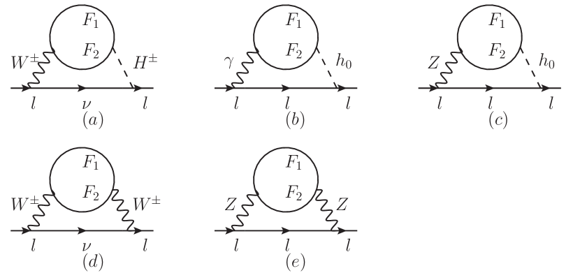
In this paper, the two-loop diagrams that we research include the Barr-Zee two-loop diagrams (FIG. 2 (a), (b), (c)) and rainbow two-loop diagrams (FIG. 2 (d), (e)), as shown below.
Figure 2: The two-loop Barr-Zee and rainbow type diagrams in the U ( 1 ) X 𝑈 subscript 1 𝑋 U(1)_{X}
The analytical results of the contributions from the two-loop diagrams to lepton EDMs are shown below.
The contribution from FIG. 2 (a). Under the assumption m F = m F 1 = m F 2 ≫ m W subscript 𝑚 𝐹 subscript 𝑚 subscript 𝐹 1 subscript 𝑚 subscript 𝐹 2 much-greater-than subscript 𝑚 𝑊 m_{F}=m_{F_{1}}=m_{F_{2}}\gg m_{W} ffa
d l W H = − G F m W 2 s W 256 π 4 ∑ F 1 = χ ± ∑ F 2 = χ 0 H l ¯ H ν L m F { ℑ [ [ 21 4 − 5 18 Q F 1 + ( 3 + Q F 1 3 ) ( ln m F 1 2 \displaystyle\qquad\quad d_{l}^{WH}=\frac{-G_{F}m_{W}^{2}s_{W}}{256\pi^{4}}\sum_{F_{1}=\chi^{\pm}}\sum_{F_{2}=\chi^{0}}\frac{H_{\bar{l}H\nu}^{L}}{m_{F}}\Big{\{}\Im\Big{[}\Big{[}\frac{21}{4}-\frac{5}{18}Q_{F_{1}}+(3+\frac{Q_{F_{1}}}{3})(\ln{m_{F_{1}}^{2}}
− ϱ 1 , 1 ( m W 2 , m H ± 2 ) ) ] ( H H F 1 F 2 L H W F 1 F 2 L + H H F 1 F 2 R H W F 1 F 2 R ) + [ 19 − 20 Q F 1 9 \displaystyle\qquad\quad-\varrho_{1,1}(m_{W}^{2},m_{H^{\pm}}^{2}))\Big{]}(H_{HF_{1}F_{2}}^{L}H_{WF_{1}F_{2}}^{L}+H_{HF_{1}F_{2}}^{R}H_{WF_{1}F_{2}}^{R})+\Big{[}\frac{19-20Q_{F_{1}}}{9}
+ 2 − 4 Q F 1 3 ( ln m F 1 2 − ϱ 1 , 1 ( m W 2 , m H ± 2 ) ) ] ( H H F 1 F 2 L H W F 1 F 2 R + H H F 1 F 2 R H W F 1 F 2 L ) \displaystyle\qquad\quad+\frac{2-4Q_{F_{1}}}{3}(\ln{m_{F_{1}}^{2}}-\varrho_{1,1}(m_{W}^{2},m_{H^{\pm}}^{2}))\Big{]}(H_{HF_{1}F_{2}}^{L}H_{WF_{1}F_{2}}^{R}+H_{HF_{1}F_{2}}^{R}H_{WF_{1}F_{2}}^{L})
+ [ − 16 9 − 2 + 6 Q F 1 3 ( ln m F 1 2 − ϱ 1 , 1 ( m W 2 , m H ± 2 ) ) ] ( H H F 1 F 2 L H W F 1 F 2 L − H H F 1 F 2 R H W F 1 F 2 R ) delimited-[] 16 9 2 6 subscript 𝑄 subscript 𝐹 1 3 superscript subscript 𝑚 subscript 𝐹 1 2 subscript italic-ϱ 1 1
superscript subscript 𝑚 𝑊 2 superscript subscript 𝑚 superscript 𝐻 plus-or-minus 2 superscript subscript 𝐻 𝐻 subscript 𝐹 1 subscript 𝐹 2 𝐿 superscript subscript 𝐻 𝑊 subscript 𝐹 1 subscript 𝐹 2 𝐿 superscript subscript 𝐻 𝐻 subscript 𝐹 1 subscript 𝐹 2 𝑅 superscript subscript 𝐻 𝑊 subscript 𝐹 1 subscript 𝐹 2 𝑅 \displaystyle\qquad\quad+\Big{[}-\frac{16}{9}-\frac{2+6Q_{F_{1}}}{3}(\ln{m_{F_{1}}^{2}}-\varrho_{1,1}(m_{W}^{2},m_{H^{\pm}}^{2}))\Big{]}(H_{HF_{1}F_{2}}^{L}H_{WF_{1}F_{2}}^{L}-H_{HF_{1}F_{2}}^{R}H_{WF_{1}F_{2}}^{R})
+ [ − 2 Q F 1 9 − 6 − 2 Q F 1 3 ( ln m F 1 2 − ϱ 1 , 1 ( m W 2 , m H ± 2 ) ) ] ( H H F 1 F 2 L H W F 1 F 2 R − H H F 1 F 2 R H W F 1 F 2 L ) ] } . \displaystyle\qquad\quad+\Big{[}-\frac{2Q_{F_{1}}}{9}-\frac{6-2Q_{F_{1}}}{3}(\ln{m_{F_{1}}^{2}}-\varrho_{1,1}(m_{W}^{2},m_{H^{\pm}}^{2}))\Big{]}(H_{HF_{1}F_{2}}^{L}H_{WF_{1}F_{2}}^{R}-H_{HF_{1}F_{2}}^{R}H_{WF_{1}F_{2}}^{L})\Big{]}\Big{\}}\;. (37)
Here, ϱ 1 , 1 ( x , y ) = x ln x − y ln y x − y subscript italic-ϱ 1 1
𝑥 𝑦 𝑥 𝑥 𝑦 𝑦 𝑥 𝑦 \varrho_{1,1}(x,y)=\frac{x\ln x-y\ln y}{x-y} H H F 1 F 2 L , R superscript subscript 𝐻 𝐻 subscript 𝐹 1 subscript 𝐹 2 𝐿 𝑅
H_{HF_{1}F_{2}}^{L,R} H W F 1 F 2 L , R superscript subscript 𝐻 𝑊 subscript 𝐹 1 subscript 𝐹 2 𝐿 𝑅
H_{WF_{1}F_{2}}^{L,R} slh
Under the assumption m F = m F 1 = m F 2 ≫ m h 0 subscript 𝑚 𝐹 subscript 𝑚 subscript 𝐹 1 subscript 𝑚 subscript 𝐹 2 much-greater-than subscript 𝑚 subscript ℎ 0 m_{F}=m_{F_{1}}=m_{F_{2}}\gg m_{h_{0}}
d l γ h 0 = − e G F Q f Q F 1 m W 2 s W 2 32 π 4 ∑ F 1 = F 2 = χ ± { ℑ [ 1 m F 1 ( H h 0 F 1 F 2 L ) [ 1 + ln m F 1 2 m h 0 2 ] ] } . superscript subscript 𝑑 𝑙 𝛾 subscript ℎ 0 𝑒 subscript 𝐺 𝐹 subscript 𝑄 𝑓 subscript 𝑄 subscript 𝐹 1 superscript subscript 𝑚 𝑊 2 superscript subscript 𝑠 𝑊 2 32 superscript 𝜋 4 subscript subscript 𝐹 1 subscript 𝐹 2 superscript 𝜒 plus-or-minus 1 subscript 𝑚 subscript 𝐹 1 superscript subscript 𝐻 subscript ℎ 0 subscript 𝐹 1 subscript 𝐹 2 𝐿 delimited-[] 1 superscript subscript 𝑚 subscript 𝐹 1 2 superscript subscript 𝑚 subscript ℎ 0 2 \displaystyle d_{l}^{\gamma h_{0}}=\frac{-eG_{F}Q_{f}Q_{F_{1}}m_{W}^{2}s_{W}^{2}}{32\pi^{4}}\sum_{F_{1}=F_{2}=\chi^{\pm}}\Big{\{}\Im\Big{[}\frac{1}{m_{F_{1}}}(H_{h_{0}F_{1}F_{2}}^{L})[1+\ln\frac{m_{F_{1}}^{2}}{m_{h_{0}}^{2}}]\Big{]}\Big{\}}\;. (38)
And, the simplified form from FIG. 2(c) is given below
d l Z h 0 = − 2 e 1024 π 4 ∑ F 1 = F 2 = χ ± , χ 0 { H h 0 l l ¯ m F 1 [ ϱ 1 , 1 ( m Z 2 , m h 0 2 ) − ln m F 1 2 − 1 ] \displaystyle d_{l}^{Zh_{0}}=\frac{-\sqrt{2}e}{1024\pi^{4}}\sum_{F_{1}=F_{2}=\chi^{\pm},\chi^{0}}\Big{\{}\frac{H_{h_{0}l\bar{l}}}{m_{F_{1}}}\Big{[}\varrho_{1,1}(m_{Z}^{2},m_{h_{0}}^{2})-\ln{m_{F_{1}}^{2}}-1\Big{]}
× ℑ [ ( H Z l l L − H Z l l R ) ( H h 0 F 1 F 2 L H Z F 1 F 2 L + H h 0 F 1 F 2 R H Z F 1 F 2 R ) ] } . \displaystyle\qquad\quad\times\Im[(H^{L}_{Zll}-H^{R}_{Zll})(H_{h_{0}F_{1}F_{2}}^{L}H_{ZF_{1}F_{2}}^{L}+H_{h_{0}F_{1}F_{2}}^{R}H_{ZF_{1}F_{2}}^{R})]\Big{\}}\;. (39)
With Q f subscript 𝑄 𝑓 Q_{f} m μ subscript 𝑚 𝜇 m_{\mu} Q F 1 subscript 𝑄 subscript 𝐹 1 Q_{F_{1}} Q F 2 subscript 𝑄 subscript 𝐹 2 Q_{F_{2}}
With the assumption m F = m F 1 = m F 2 ≫ m W ∼ m Z subscript 𝑚 𝐹 subscript 𝑚 subscript 𝐹 1 subscript 𝑚 subscript 𝐹 2 much-greater-than subscript 𝑚 𝑊 similar-to subscript 𝑚 𝑍 m_{F}=m_{F_{1}}=m_{F_{2}}\gg m_{W}\sim m_{Z}
d l W W = − e G F m l 384 2 π 4 ∑ F 1 = χ ± ∑ F 2 = χ 0 { ℑ [ 11 ( H W F 1 F 2 R ∗ H W F 1 F 2 L ) ] } . superscript subscript 𝑑 𝑙 𝑊 𝑊 𝑒 subscript 𝐺 𝐹 subscript 𝑚 𝑙 384 2 superscript 𝜋 4 subscript subscript 𝐹 1 superscript 𝜒 plus-or-minus subscript subscript 𝐹 2 superscript 𝜒 0 11 superscript subscript 𝐻 𝑊 subscript 𝐹 1 subscript 𝐹 2 𝑅
superscript subscript 𝐻 𝑊 subscript 𝐹 1 subscript 𝐹 2 𝐿 \displaystyle d_{l}^{WW}=\frac{-eG_{F}m_{l}}{384\sqrt{2}\pi^{4}}\sum_{F_{1}=\chi^{\pm}}\sum_{F_{2}=\chi^{0}}\left\{\Im[11(H_{WF_{1}F_{2}}^{R*}H_{WF_{1}F_{2}}^{L})]\right\}\;. (40)
We simplify the tedious two-loop results to the order m μ 2 M Z 2 superscript subscript 𝑚 𝜇 2 superscript subscript 𝑀 𝑍 2 \frac{m_{\mu}^{2}}{M_{Z}^{2}} ∼ similar-to \sim 10 − 6 superscript 10 6 10^{-6} m μ 2 m S U S Y 2 superscript subscript 𝑚 𝜇 2 superscript subscript 𝑚 𝑆 𝑈 𝑆 𝑌 2 \frac{m_{\mu}^{2}}{m_{SUSY}^{2}} m F = m F 1 = m F 2 ≫ m W ∼ m Z subscript 𝑚 𝐹 subscript 𝑚 𝐹 1 subscript 𝑚 𝐹 2 much-greater-than subscript 𝑚 𝑊 similar-to subscript 𝑚 𝑍 m_{F}=m_{F1}=m_{F2}\gg m_{W}\sim m_{Z}
d l Z Z = e Q F 1 m l 2048 Λ 2 π 4 ∑ F 1 = F 2 = χ ± { ℑ [ ( H Z F 1 F 2 L H Z F 1 F 2 R ) ( | H Z l l L | 2 + | H Z l l R | 2 ) [ − 6 log x Z + 6 log x F + 4 9 x F ] \displaystyle d_{l}^{ZZ}=\frac{eQ_{F_{1}}m_{l}}{2048\Lambda^{2}\pi^{4}}\sum_{F_{1}=F_{2}=\chi^{\pm}}\Big{\{}\Im\Big{[}(H^{L}_{ZF_{1}F_{2}}H^{R}_{ZF_{1}F_{2}})\Big{(}|H^{L}_{Zll}|^{2}+|H^{R}_{Zll}|^{2}\Big{)}[\frac{-6\log x_{Z}+6\log x_{F}+4}{9x_{F}}]
+ ( | H Z F 1 F 2 L | 2 + | H Z F 1 F 2 R | 2 ) H Z l l L H Z l l R [ 16 ( log x F − log x Z ) ( log x F + 2 ) + 2 x Z ] ] } . \displaystyle+\Big{(}|H^{L}_{ZF_{1}F_{2}}|^{2}+|H^{R}_{ZF_{1}F_{2}}|^{2}\Big{)}H^{L}_{Zll}H^{R}_{Zll}[16\frac{(\log x_{F}-\log x_{Z})(\log x_{F}+2)+2}{x_{Z}}]\Big{]}\Big{\}}\;. (41)
The contributions to lepton EDMs from the researched two-loop diagrams are
d l t w o − l o o p = d l W H + d l γ h 0 + d l Z h 0 + d l W W + d l Z Z . superscript subscript 𝑑 𝑙 𝑡 𝑤 𝑜 𝑙 𝑜 𝑜 𝑝 superscript subscript 𝑑 𝑙 𝑊 𝐻 superscript subscript 𝑑 𝑙 𝛾 subscript ℎ 0 superscript subscript 𝑑 𝑙 𝑍 subscript ℎ 0 superscript subscript 𝑑 𝑙 𝑊 𝑊 superscript subscript 𝑑 𝑙 𝑍 𝑍 \displaystyle d_{l}^{two-loop}=d_{l}^{WH}+d_{l}^{\gamma h_{0}}+d_{l}^{Zh_{0}}+d_{l}^{WW}+d_{l}^{ZZ}\;. (42)
At two-loop level, the contributions to lepton EDMs can be summarized as
d l t o t a l = d l o n e − l o o p + d l t w o − l o o p . superscript subscript 𝑑 𝑙 𝑡 𝑜 𝑡 𝑎 𝑙 superscript subscript 𝑑 𝑙 𝑜 𝑛 𝑒 𝑙 𝑜 𝑜 𝑝 superscript subscript 𝑑 𝑙 𝑡 𝑤 𝑜 𝑙 𝑜 𝑜 𝑝 \displaystyle d_{l}^{total}=d_{l}^{one-loop}+d_{l}^{two-loop}\;. (43)
IV the numerical results
For the numerical discussion, we consider the following experimental limitations. The lightest CP-even higgs mass is considered as an input parameter, which is m h 0 subscript 𝑚 superscript ℎ 0 m_{h^{0}} ≈ \approx hmass1 ; hmass2 h 0 superscript ℎ 0 h^{0} h 0 → γ + γ → superscript ℎ 0 𝛾 𝛾 h^{0}\rightarrow\gamma+\gamma h 0 → Z + Z → superscript ℎ 0 𝑍 𝑍 h^{0}\rightarrow Z+Z h 0 → γ + γ → superscript ℎ 0 𝛾 𝛾 h^{0}\rightarrow\gamma+\gamma dec Z ′ superscript 𝑍 ′ Z^{\prime} M Z ′ subscript 𝑀 superscript 𝑍 ′ M_{Z^{\prime}} 51 M Z ′ subscript 𝑀 superscript 𝑍 ′ M_{Z^{\prime}} g X subscript 𝑔 𝑋 g_{X} ( M Z ′ g X ) subscript 𝑀 superscript 𝑍 ′ subscript 𝑔 𝑋 (\frac{M_{Z^{\prime}}}{g_{X}}) 99 % percent 99 99\% cl1 ; cl2 tan β η < 1.5 subscript 𝛽 𝜂 1.5 \tan{\beta_{\eta}}<1.5 BT M Z ′ subscript 𝑀 superscript 𝑍 ′ M_{Z^{\prime}} Z ′ superscript 𝑍 ′ Z^{\prime} Z ′ superscript 𝑍 ′ Z^{\prime} e , μ , τ 𝑒 𝜇 𝜏
e,\mu,\tau
The parameters used in U ( 1 ) X 𝑈 subscript 1 𝑋 U(1)_{X}
g X = 0.33 , g Y X = 0.2 , λ C = − 0.1 , κ = 0.1 , T λ H = 1.0 TeV , T κ = 1.0 TeV , formulae-sequence subscript 𝑔 𝑋 0.33 formulae-sequence subscript 𝑔 𝑌 𝑋 0.2 formulae-sequence subscript 𝜆 𝐶 0.1 formulae-sequence 𝜅 0.1 formulae-sequence subscript 𝑇 subscript 𝜆 𝐻 1.0 TeV subscript 𝑇 𝜅 1.0 TeV \displaystyle g_{X}=0.33,~{}g_{YX}=0.2,~{}\lambda_{C}=-0.1,~{}\kappa=0.1,~{}T_{\lambda_{H}}=1.0~{}{\rm TeV},~{}T_{\kappa}=1.0~{}{\rm TeV},
tan β η = 1.05 , v η = 15 × cos β η TeV , v η ¯ = 15 × sin β η TeV , B μ = 8 TeV 2 , formulae-sequence subscript 𝛽 𝜂 1.05 formulae-sequence subscript 𝑣 𝜂 15 subscript 𝛽 𝜂 TeV formulae-sequence subscript 𝑣 ¯ 𝜂 15 subscript 𝛽 𝜂 TeV subscript 𝐵 𝜇 8 superscript TeV 2 \displaystyle\tan{\beta_{\eta}}=1.05,~{}v_{\eta}=15\times\cos{\beta_{\eta}}~{}{\rm TeV},~{}v_{\bar{\eta}}=15\times\sin{\beta_{\eta}}~{}{\rm TeV},~{}B_{\mu}=8~{}{\rm TeV^{2}},
m S 2 = 8 TeV 2 , T λ C = 150 GeV , T E 11 = T E 22 = T E 33 = 0.1 TeV , formulae-sequence superscript subscript 𝑚 𝑆 2 8 superscript TeV 2 formulae-sequence subscript 𝑇 subscript 𝜆 𝐶 150 GeV subscript 𝑇 𝐸 11 subscript 𝑇 𝐸 22 subscript 𝑇 𝐸 33 0.1 TeV \displaystyle m_{S}^{2}=8~{}{\rm TeV^{2}},~{}T_{\lambda_{C}}=150~{}{\rm GeV},~{}T_{E11}=T_{E22}=T_{E33}=0.1~{}{\rm TeV},
M ν 11 = M ν 22 = M ν 33 = 6 TeV 2 , Y X 11 = Y X 22 = Y X 33 = 0.04 , formulae-sequence subscript 𝑀 𝜈 11 subscript 𝑀 𝜈 22 subscript 𝑀 𝜈 33 6 superscript TeV 2 subscript 𝑌 𝑋 11 subscript 𝑌 𝑋 22 subscript 𝑌 𝑋 33 0.04 \displaystyle M_{\nu 11}=M_{\nu 22}=M_{\nu 33}=6~{}{\rm TeV^{2}},~{}Y_{X11}=Y_{X22}=Y_{X33}=0.04,
B S = 8 TeV 2 , λ H = 0.1 , l W = 8 TeV 2 , T X 11 = T X 22 = T X 33 = 10 GeV . formulae-sequence subscript 𝐵 𝑆 8 superscript TeV 2 formulae-sequence subscript 𝜆 𝐻 0.1 formulae-sequence subscript 𝑙 𝑊 8 superscript TeV 2 subscript 𝑇 𝑋 11 subscript 𝑇 𝑋 22 subscript 𝑇 𝑋 33 10 GeV \displaystyle B_{S}=8~{}{\rm TeV^{2}},~{}\lambda_{H}=0.1,~{}l_{W}=8~{}{\rm TeV^{2}},~{}T_{X11}=T_{X22}=T_{X33}=10~{}{\rm GeV}. (44)
θ 1 subscript 𝜃 1 \theta_{1} θ 2 subscript 𝜃 2 \theta_{2} θ μ subscript 𝜃 𝜇 \theta_{\mu} m 1 subscript 𝑚 1 m_{1} m 2 subscript 𝑚 2 m_{2} μ 𝜇 \mu θ B L subscript 𝜃 𝐵 𝐿 \theta_{BL} θ B B ′ subscript 𝜃 𝐵 superscript 𝐵 ′ \theta_{BB^{\prime}} θ S subscript 𝜃 𝑆 \theta_{S}
m 1 = M 1 ∗ e i ∗ θ 1 , m 2 = M 2 ∗ e i ∗ θ 2 , μ = m u ∗ e i ∗ θ μ , formulae-sequence subscript 𝑚 1 subscript 𝑀 1 superscript 𝑒 𝑖 subscript 𝜃 1 formulae-sequence subscript 𝑚 2 subscript 𝑀 2 superscript 𝑒 𝑖 subscript 𝜃 2 𝜇 𝑚 𝑢 superscript 𝑒 𝑖 subscript 𝜃 𝜇 \displaystyle m_{1}=M_{1}*e^{i*\theta_{1}},~{}m_{2}=M_{2}*e^{i*\theta_{2}},~{}\mu=mu*e^{i*\theta_{\mu}},
m B L = M B L ∗ e i ∗ θ B L , m B B ′ = M B B ′ ∗ e i ∗ θ B B ′ , m S = M S ∗ e i ∗ θ S . formulae-sequence subscript 𝑚 𝐵 𝐿 subscript 𝑀 𝐵 𝐿 superscript 𝑒 𝑖 subscript 𝜃 𝐵 𝐿 formulae-sequence subscript 𝑚 𝐵 superscript 𝐵 ′ subscript 𝑀 𝐵 superscript 𝐵 ′ superscript 𝑒 𝑖 subscript 𝜃 𝐵 superscript 𝐵 ′ subscript 𝑚 𝑆 subscript 𝑀 𝑆 superscript 𝑒 𝑖 subscript 𝜃 𝑆 \displaystyle m_{BL}=M_{BL}*e^{i*\theta_{BL}},~{}m_{{BB}^{\prime}}=M_{{BB}^{\prime}}*e^{i*\theta_{BB^{\prime}}},~{}m_{S}=M_{S}*e^{i*\theta_{S}}. (45)
In order to facilitate the following discussion, we have made some simplifications:
M L = M L 11 = M L 22 = M L 33 , M E = M E 11 = M E 22 = M E 33 , formulae-sequence subscript 𝑀 𝐿 subscript 𝑀 𝐿 11 subscript 𝑀 𝐿 22 subscript 𝑀 𝐿 33 subscript 𝑀 𝐸 subscript 𝑀 𝐸 11 subscript 𝑀 𝐸 22 subscript 𝑀 𝐸 33 \displaystyle M_{L}=M_{L11}=M_{L22}=M_{L33},~{}~{}~{}M_{E}=M_{E11}=M_{E22}=M_{E33},
T E = T E 11 = T E 22 = T E 33 . subscript 𝑇 𝐸 subscript 𝑇 𝐸 11 subscript 𝑇 𝐸 22 subscript 𝑇 𝐸 33 \displaystyle T_{E}=T_{E11}=T_{E22}=T_{E33}. (46)
IV.1 the e EDM
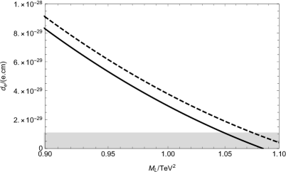
At the beginning, we discussed the EDM of electron, because its experimental upper limit is very strict. The CP violating phases θ 1 subscript 𝜃 1 \theta_{1} θ 2 subscript 𝜃 2 \theta_{2} θ μ subscript 𝜃 𝜇 \theta_{\mu} θ B L subscript 𝜃 𝐵 𝐿 \theta_{BL} θ B B ′ subscript 𝜃 𝐵 superscript 𝐵 ′ \theta_{BB^{\prime}} θ S subscript 𝜃 𝑆 \theta_{S} θ 1 subscript 𝜃 1 \theta_{1} θ 2 subscript 𝜃 2 \theta_{2} θ μ subscript 𝜃 𝜇 \theta_{\mu} θ B B ′ subscript 𝜃 𝐵 superscript 𝐵 ′ \theta_{BB^{\prime}} θ S subscript 𝜃 𝑆 \theta_{S} tan β = 5 𝛽 5 \tan{\beta}=5 M 2 = 500 GeV subscript 𝑀 2 500 GeV M_{2}=500~{}{\rm GeV} m u = 500 GeV 𝑚 𝑢 500 GeV mu=500~{}{\rm GeV} M B L = 1800 GeV subscript 𝑀 𝐵 𝐿 1800 GeV M_{BL}=1800~{}{\rm GeV} M B B ′ = 700 GeV subscript 𝑀 𝐵 superscript 𝐵 ′ 700 GeV M_{BB^{\prime}}=700~{}{\rm GeV} M S = 2400 GeV subscript 𝑀 𝑆 2400 GeV M_{S}=2400~{}{\rm GeV} M L = 1.1 TeV subscript 𝑀 𝐿 1.1 TeV M_{L}=1.1~{}{\rm TeV} M E = 1.0 TeV subscript 𝑀 𝐸 1.0 TeV M_{E}=1.0~{}{\rm TeV} θ B L subscript 𝜃 𝐵 𝐿 \theta_{BL} M B L subscript 𝑀 𝐵 𝐿 M_{BL} 3 M L subscript 𝑀 𝐿 M_{L} 0.9 ∼ 1.1 TeV 2 similar-to 0.9 1.1 superscript TeV 2 0.9\sim 1.1~{}{\rm TeV^{2}} M 1 subscript 𝑀 1 M_{1} 700 , 800 GeV 700 800 GeV
700,800~{}{\rm GeV} θ B L subscript 𝜃 𝐵 𝐿 \theta_{BL} | d e | subscript 𝑑 𝑒 |d_{e}| d e subscript 𝑑 𝑒 d_{e} M L subscript 𝑀 𝐿 M_{L} M L − 2 superscript subscript 𝑀 𝐿 2 M_{L}^{-2}
Figure 3: With θ 1 subscript 𝜃 1 \theta_{1} θ 2 subscript 𝜃 2 \theta_{2} θ μ subscript 𝜃 𝜇 \theta_{\mu} θ B B ′ subscript 𝜃 𝐵 superscript 𝐵 ′ \theta_{BB^{\prime}} θ S subscript 𝜃 𝑆 \theta_{S} θ B L subscript 𝜃 𝐵 𝐿 \theta_{BL} π 4 𝜋 4 \frac{\pi}{4} M L subscript 𝑀 𝐿 M_{L} M 1 subscript 𝑀 1 M_{1} 700 , 800 ) GeV 700,800)~{}{\rm GeV}
Figure 4: With θ 1 subscript 𝜃 1 \theta_{1} θ 2 subscript 𝜃 2 \theta_{2} θ μ subscript 𝜃 𝜇 \theta_{\mu} θ B B ′ subscript 𝜃 𝐵 superscript 𝐵 ′ \theta_{BB^{\prime}} θ B L subscript 𝜃 𝐵 𝐿 \theta_{BL} θ S subscript 𝜃 𝑆 \theta_{S} π 4 𝜋 4 \frac{\pi}{4} M L 11 subscript 𝑀 𝐿 11 M_{L11} M L 33 subscript 𝑀 𝐿 33 M_{L33} ( 1 , 0.9 ) TeV 2 1 0.9 superscript TeV 2 (1,0.9)~{}{\rm TeV^{2}}
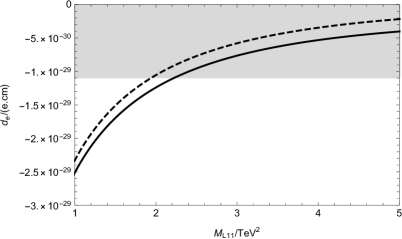
Setting θ 1 subscript 𝜃 1 \theta_{1} θ 2 subscript 𝜃 2 \theta_{2} θ μ subscript 𝜃 𝜇 \theta_{\mu} θ B B ′ subscript 𝜃 𝐵 superscript 𝐵 ′ \theta_{BB^{\prime}} θ B L subscript 𝜃 𝐵 𝐿 \theta_{BL} tan β = 5 𝛽 5 \tan{\beta}=5 M 1 = 700 GeV subscript 𝑀 1 700 GeV M_{1}=700~{}{\rm GeV} M 2 = 2000 GeV subscript 𝑀 2 2000 GeV M_{2}=2000~{}{\rm GeV} m u = 500 GeV 𝑚 𝑢 500 GeV mu=500~{}{\rm GeV} M B L = 1600 GeV subscript 𝑀 𝐵 𝐿 1600 GeV M_{BL}=1600~{}{\rm GeV} M B B ′ = 800 GeV subscript 𝑀 𝐵 superscript 𝐵 ′ 800 GeV M_{BB^{\prime}}=800~{}{\rm GeV} M S = − 800 GeV subscript 𝑀 𝑆 800 GeV M_{S}=-800~{}{\rm GeV} M L 22 = 1.0 TeV 2 subscript 𝑀 𝐿 22 1.0 superscript TeV 2 M_{L22}=1.0~{}{\rm TeV^{2}} M E = 1.0 TeV 2 subscript 𝑀 𝐸 1.0 superscript TeV 2 M_{E}=1.0~{}{\rm TeV^{2}} θ S subscript 𝜃 𝑆 \theta_{S} M S subscript 𝑀 𝑆 M_{S} 4 M L 11 subscript 𝑀 𝐿 11 M_{L11} 0.5 0.5 0.5 5.0 5.0 5.0 TeV 2 superscript TeV 2 ~{}{\rm TeV^{2}} M L 11 subscript 𝑀 𝐿 11 M_{L11} > > 2.0 TeV 2 2.0 superscript TeV 2 2.0~{}{\rm TeV^{2}} | d e | subscript 𝑑 𝑒 |d_{e}|
Figure 5: With θ 1 subscript 𝜃 1 \theta_{1} θ 2 subscript 𝜃 2 \theta_{2} θ μ subscript 𝜃 𝜇 \theta_{\mu} θ S subscript 𝜃 𝑆 \theta_{S} θ B L subscript 𝜃 𝐵 𝐿 \theta_{BL} θ B B ′ subscript 𝜃 𝐵 superscript 𝐵 ′ \theta_{BB^{\prime}} π 3 𝜋 3 \frac{\pi}{3} T E subscript 𝑇 𝐸 T_{E} M E 11 subscript 𝑀 𝐸 11 M_{E11} ( 0.5 , 1.0 ) TeV 2 0.5 1.0 superscript TeV 2 (0.5,1.0)~{}{\rm TeV^{2}}
θ B B ′ subscript 𝜃 𝐵 superscript 𝐵 ′ \theta_{BB^{\prime}} θ 1 subscript 𝜃 1 \theta_{1} θ 2 subscript 𝜃 2 \theta_{2} θ μ subscript 𝜃 𝜇 \theta_{\mu} θ S subscript 𝜃 𝑆 \theta_{S} θ B L subscript 𝜃 𝐵 𝐿 \theta_{BL} T E subscript 𝑇 𝐸 T_{E} M E 11 subscript 𝑀 𝐸 11 M_{E11} TeV 2 superscript TeV 2 ~{}{\rm TeV^{2}} tan β = 5 𝛽 5 \tan{\beta}=5 M 1 = 700 GeV subscript 𝑀 1 700 GeV M_{1}=700~{}{\rm GeV} M 2 = 2000 GeV subscript 𝑀 2 2000 GeV M_{2}=2000~{}{\rm GeV} m u = 500 GeV 𝑚 𝑢 500 GeV mu=500~{}{\rm GeV} M B L = 1800 GeV subscript 𝑀 𝐵 𝐿 1800 GeV M_{BL}=1800~{}{\rm GeV} M B B ′ = 700 GeV subscript 𝑀 𝐵 superscript 𝐵 ′ 700 GeV M_{BB^{\prime}}=700~{}{\rm GeV} M S = 2400 GeV subscript 𝑀 𝑆 2400 GeV M_{S}=2400~{}{\rm GeV} M L = 1.0 TeV 2 subscript 𝑀 𝐿 1.0 superscript TeV 2 M_{L}=1.0~{}{\rm TeV^{2}} M E = 0.5 TeV 2 subscript 𝑀 𝐸 0.5 superscript TeV 2 M_{E}=0.5~{}{\rm TeV^{2}} 5
Figure 6: With θ 1 subscript 𝜃 1 \theta_{1} θ 2 subscript 𝜃 2 \theta_{2} θ μ subscript 𝜃 𝜇 \theta_{\mu} θ B B ′ subscript 𝜃 𝐵 superscript 𝐵 ′ \theta_{BB^{\prime}} θ B L subscript 𝜃 𝐵 𝐿 \theta_{BL} θ S subscript 𝜃 𝑆 \theta_{S} π 4 𝜋 4 \frac{\pi}{4} | d e | subscript 𝑑 𝑒 |d_{e}| M L 11 subscript 𝑀 𝐿 11 M_{L11} M L 22 subscript 𝑀 𝐿 22 M_{L22} ■ ■ \blacksquare | d e | < 1.1 × 10 − 29 subscript 𝑑 𝑒 1.1 superscript 10 29 |d_{e}|<1.1\times 10^{-29} ∘ \circ | d e | ⩾ 1.1 × 10 − 29 subscript 𝑑 𝑒 1.1 superscript 10 29 |d_{e}|\geqslant 1.1\times 10^{-29}
We select these parameters M L 11 ( 0.5 ∼ 5.0 TeV 2 ) subscript 𝑀 𝐿 11 ∼ 0.5 5.0 superscript TeV 2 M_{L11}(0.5\thicksim 5.0~{}{\rm TeV^{2}}) M L 22 ( 0.5 ∼ 5.0 TeV 2 ) subscript 𝑀 𝐿 22 ∼ 0.5 5.0 superscript TeV 2 M_{L22}(0.5\thicksim 5.0~{}{\rm TeV^{2}}) M L 33 ( 0.5 ∼ 5.0 TeV 2 ) subscript 𝑀 𝐿 33 ∼ 0.5 5.0 superscript TeV 2 M_{L33}(0.5\thicksim 5.0~{}{\rm TeV^{2}}) T E ( − 3000 ∼ 3000 GeV ) subscript 𝑇 𝐸 ∼ 3000 3000 GeV T_{E}(-3000\thicksim 3000~{}{\rm GeV}) M E ( 0.5 ∼ 5.0 TeV 2 ) subscript 𝑀 𝐸 ∼ 0.5 5.0 superscript TeV 2 M_{E}(0.5\thicksim 5.0~{}{\rm TeV^{2}}) θ 1 subscript 𝜃 1 \theta_{1} θ 2 subscript 𝜃 2 \theta_{2} θ μ subscript 𝜃 𝜇 \theta_{\mu} θ B B ′ subscript 𝜃 𝐵 superscript 𝐵 ′ \theta_{BB^{\prime}} θ B L subscript 𝜃 𝐵 𝐿 \theta_{BL} θ S subscript 𝜃 𝑆 \theta_{S} π 4 𝜋 4 \frac{\pi}{4} | d e | subscript 𝑑 𝑒 |d_{e}| M L 11 subscript 𝑀 𝐿 11 M_{L11} M L 22 subscript 𝑀 𝐿 22 M_{L22} 6 ■ ■ \blacksquare | d e | < 1.1 × 10 − 29 subscript 𝑑 𝑒 1.1 superscript 10 29 |d_{e}|<1.1\times 10^{-29} ∘ \circ | d e | ⩾ 1.1 × 10 − 29 subscript 𝑑 𝑒 1.1 superscript 10 29 |d_{e}|\geqslant 1.1\times 10^{-29} 6 M L 11 subscript 𝑀 𝐿 11 M_{L11} > > TeV 2 superscript TeV 2 ~{}{\rm TeV^{2}} M L 22 subscript 𝑀 𝐿 22 M_{L22} TeV 2 superscript TeV 2 ~{}{\rm TeV^{2}} | d e | subscript 𝑑 𝑒 |d_{e}| M L 11 subscript 𝑀 𝐿 11 M_{L11} M L 22 subscript 𝑀 𝐿 22 M_{L22}
IV.2 the μ 𝜇 \mu
In this section, the muon EDM is numerically studied. In FIG. 7 θ 1 subscript 𝜃 1 \theta_{1} θ μ subscript 𝜃 𝜇 \theta_{\mu} θ B B ′ subscript 𝜃 𝐵 superscript 𝐵 ′ \theta_{BB^{\prime}} θ 2 subscript 𝜃 2 \theta_{2} θ B L subscript 𝜃 𝐵 𝐿 \theta_{BL} tan β = 6 𝛽 6 \tan{\beta}=6 M 1 = 1450 GeV subscript 𝑀 1 1450 GeV M_{1}=1450~{}{\rm GeV} M 2 = 2000 GeV subscript 𝑀 2 2000 GeV M_{2}=2000~{}{\rm GeV} m u = 500 GeV 𝑚 𝑢 500 GeV mu=500~{}{\rm GeV} M B B ′ = 800 GeV subscript 𝑀 𝐵 superscript 𝐵 ′ 800 GeV M_{BB^{\prime}}=800~{}{\rm GeV} M S = − 800 GeV subscript 𝑀 𝑆 800 GeV M_{S}=-800~{}{\rm GeV} M L = 1.0 TeV 2 subscript 𝑀 𝐿 1.0 superscript TeV 2 M_{L}=1.0~{}{\rm TeV^{2}} M E = 0.5 TeV 2 subscript 𝑀 𝐸 0.5 superscript TeV 2 M_{E}=0.5~{}{\rm TeV^{2}} θ S subscript 𝜃 𝑆 \theta_{S} M B L subscript 𝑀 𝐵 𝐿 M_{BL} 1200 , 1500 GeV 1200 1500 GeV
1200,1500~{}{\rm GeV} M E subscript 𝑀 𝐸 M_{E} θ S subscript 𝜃 𝑆 \theta_{S} M S subscript 𝑀 𝑆 M_{S}
Figure 7: With θ 1 subscript 𝜃 1 \theta_{1} θ 2 subscript 𝜃 2 \theta_{2} θ μ subscript 𝜃 𝜇 \theta_{\mu} θ B B ′ subscript 𝜃 𝐵 superscript 𝐵 ′ \theta_{BB^{\prime}} θ B L subscript 𝜃 𝐵 𝐿 \theta_{BL} θ S subscript 𝜃 𝑆 \theta_{S} π 3 𝜋 3 \frac{\pi}{3} M E subscript 𝑀 𝐸 M_{E} M B L subscript 𝑀 𝐵 𝐿 M_{BL} ( 1200 , 1500 ) GeV 1200 1500 GeV (1200,1500)~{}{\rm GeV}
θ B B ′ subscript 𝜃 𝐵 superscript 𝐵 ′ \theta_{BB^{\prime}} θ 1 subscript 𝜃 1 \theta_{1} θ 2 subscript 𝜃 2 \theta_{2} θ μ subscript 𝜃 𝜇 \theta_{\mu} θ S subscript 𝜃 𝑆 \theta_{S} θ B L subscript 𝜃 𝐵 𝐿 \theta_{BL} M E 22 subscript 𝑀 𝐸 22 M_{E22} tan β 𝛽 \tan\beta M 1 = 1450 GeV subscript 𝑀 1 1450 GeV M_{1}=1450~{}{\rm GeV} M 2 = 800 GeV subscript 𝑀 2 800 GeV M_{2}=800~{}{\rm GeV} m u = 500 GeV 𝑚 𝑢 500 GeV mu=500~{}{\rm GeV} M B L = 1600 GeV subscript 𝑀 𝐵 𝐿 1600 GeV M_{BL}=1600~{}{\rm GeV} M B B ′ = 800 GeV subscript 𝑀 𝐵 superscript 𝐵 ′ 800 GeV M_{BB^{\prime}}=800~{}{\rm GeV} M S = − 800 GeV subscript 𝑀 𝑆 800 GeV M_{S}=-800~{}{\rm GeV} M L = 1.0 TeV 2 subscript 𝑀 𝐿 1.0 superscript TeV 2 M_{L}=1.0~{}{\rm TeV^{2}} M E = 0.5 TeV 2 subscript 𝑀 𝐸 0.5 superscript TeV 2 M_{E}=0.5~{}{\rm TeV^{2}} 8 M E 22 subscript 𝑀 𝐸 22 M_{E22}
Figure 8: With θ 1 subscript 𝜃 1 \theta_{1} θ 2 subscript 𝜃 2 \theta_{2} θ μ subscript 𝜃 𝜇 \theta_{\mu} θ S subscript 𝜃 𝑆 \theta_{S} θ B L subscript 𝜃 𝐵 𝐿 \theta_{BL} θ B B ′ subscript 𝜃 𝐵 superscript 𝐵 ′ \theta_{BB^{\prime}} π 6 𝜋 6 \frac{\pi}{6} M E 22 subscript 𝑀 𝐸 22 M_{E22} tan β 𝛽 \tan\beta 5 , 6 5 6
5,6
We choose these parameters M L 11 ( 0.5 ∼ 5.0 TeV 2 ) subscript 𝑀 𝐿 11 ∼ 0.5 5.0 superscript TeV 2 M_{L11}(0.5\thicksim 5.0~{}{\rm TeV^{2}}) M L 22 ( 0.5 ∼ 5.0 TeV 2 ) subscript 𝑀 𝐿 22 ∼ 0.5 5.0 superscript TeV 2 M_{L22}(0.5\thicksim 5.0~{}{\rm TeV^{2}}) M L 33 ( 0.5 ∼ 5.0 TeV 2 ) subscript 𝑀 𝐿 33 ∼ 0.5 5.0 superscript TeV 2 M_{L33}(0.5\thicksim 5.0~{}{\rm TeV^{2}}) T E ( − 3000 ∼ 3000 GeV ) subscript 𝑇 𝐸 ∼ 3000 3000 GeV T_{E}(-3000\thicksim 3000~{}{\rm GeV}) M E ( 0.5 ∼ 5.0 TeV 2 ) subscript 𝑀 𝐸 ∼ 0.5 5.0 superscript TeV 2 M_{E}(0.5\thicksim 5.0~{}{\rm TeV^{2}}) θ 1 subscript 𝜃 1 \theta_{1} θ 2 subscript 𝜃 2 \theta_{2} θ μ subscript 𝜃 𝜇 \theta_{\mu} θ B B ′ subscript 𝜃 𝐵 superscript 𝐵 ′ \theta_{BB^{\prime}} θ B L subscript 𝜃 𝐵 𝐿 \theta_{BL} θ S subscript 𝜃 𝑆 \theta_{S} π 4 𝜋 4 \frac{\pi}{4} | d μ | subscript 𝑑 𝜇 |d_{\mu}| M L 33 subscript 𝑀 𝐿 33 M_{L33} M E subscript 𝑀 𝐸 M_{E} 9 ■ ■ \blacksquare | d μ | subscript 𝑑 𝜇 |d_{\mu}| < < 1 × 10 − 24 1 superscript 10 24 1\times 10^{-24} ∘ \circ | d μ | subscript 𝑑 𝜇 |d_{\mu}| ⩾ \geqslant 1 × 10 − 24 1 superscript 10 24 1\times 10^{-24} M E subscript 𝑀 𝐸 M_{E} 1.1 TeV 2 1.1 superscript TeV 2 1.1~{}{\rm TeV^{2}} M E subscript 𝑀 𝐸 M_{E} M L 33 subscript 𝑀 𝐿 33 M_{L33}
Figure 9: With θ 1 subscript 𝜃 1 \theta_{1} θ 2 subscript 𝜃 2 \theta_{2} θ μ subscript 𝜃 𝜇 \theta_{\mu} θ B B ′ subscript 𝜃 𝐵 superscript 𝐵 ′ \theta_{BB^{\prime}} θ B L subscript 𝜃 𝐵 𝐿 \theta_{BL} θ S subscript 𝜃 𝑆 \theta_{S} π 4 𝜋 4 \frac{\pi}{4} | d μ | subscript 𝑑 𝜇 |d_{\mu}| M L 33 subscript 𝑀 𝐿 33 M_{L33} M E subscript 𝑀 𝐸 M_{E} ■ ■ \blacksquare | d μ | subscript 𝑑 𝜇 |d_{\mu}| < < 1 × 10 − 24 1 superscript 10 24 1\times 10^{-24} ∘ \circ | d μ | subscript 𝑑 𝜇 |d_{\mu}| ⩾ \geqslant 1 × 10 − 24 1 superscript 10 24 1\times 10^{-24}
IV.3 the τ 𝜏 \tau
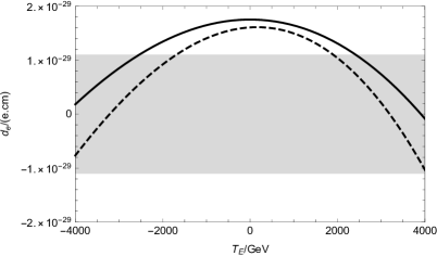
At present, the experimental upper bound of tau EDM is | d τ e x p | subscript superscript 𝑑 𝑒 𝑥 𝑝 𝜏 |d^{exp}_{\tau}| < < 1.1 × 10 − 17 1.1 superscript 10 17 1.1\times 10^{-17} tan β = 6 𝛽 6 \tan{\beta}=6 M 1 = 750 GeV subscript 𝑀 1 750 GeV M_{1}=750~{}{\rm GeV} m u = 650 GeV 𝑚 𝑢 650 GeV mu=650~{}{\rm GeV} M B L = 1800 GeV subscript 𝑀 𝐵 𝐿 1800 GeV M_{BL}=1800~{}{\rm GeV} M B B ′ = 700 GeV subscript 𝑀 𝐵 superscript 𝐵 ′ 700 GeV M_{BB^{\prime}}=700~{}{\rm GeV} M S = 1400 GeV subscript 𝑀 𝑆 1400 GeV M_{S}=1400~{}{\rm GeV} M L = 1.0 TeV 2 subscript 𝑀 𝐿 1.0 superscript TeV 2 M_{L}=1.0~{}{\rm TeV^{2}} M E = 1.0 TeV 2 subscript 𝑀 𝐸 1.0 superscript TeV 2 M_{E}=1.0~{}{\rm TeV^{2}} θ 1 subscript 𝜃 1 \theta_{1} θ 2 subscript 𝜃 2 \theta_{2} θ μ subscript 𝜃 𝜇 \theta_{\mu} θ B B ′ subscript 𝜃 𝐵 superscript 𝐵 ′ \theta_{BB^{\prime}} θ B L subscript 𝜃 𝐵 𝐿 \theta_{BL} θ S subscript 𝜃 𝑆 \theta_{S} π 5 𝜋 5 \frac{\pi}{5} M L 33 subscript 𝑀 𝐿 33 M_{L33} | d τ | subscript 𝑑 𝜏 |d_{\tau}| 10 M 2 subscript 𝑀 2 M_{2} ( 400 , 500 GeV ) 400 500 GeV (400,500~{}{\rm GeV}) M L 33 subscript 𝑀 𝐿 33 M_{L33} θ S subscript 𝜃 𝑆 \theta_{S} | d τ | subscript 𝑑 𝜏 |d_{\tau}| 5.0 × 10 − 23 5.0 superscript 10 23 5.0\times 10^{-23}
Figure 10: With θ 1 subscript 𝜃 1 \theta_{1} θ 2 subscript 𝜃 2 \theta_{2} θ μ subscript 𝜃 𝜇 \theta_{\mu} θ B B ′ subscript 𝜃 𝐵 superscript 𝐵 ′ \theta_{BB^{\prime}} θ B L subscript 𝜃 𝐵 𝐿 \theta_{BL} θ S subscript 𝜃 𝑆 \theta_{S} π 5 𝜋 5 \frac{\pi}{5} M L 33 subscript 𝑀 𝐿 33 M_{L33} M 2 subscript 𝑀 2 M_{2} ( 400 , 500 ) GeV 400 500 GeV (400,500)~{}{\rm GeV}
θ B L subscript 𝜃 𝐵 𝐿 \theta_{BL} M B L subscript 𝑀 𝐵 𝐿 M_{BL} tan β = 6 𝛽 6 \tan{\beta}=6 M 1 = 750 GeV subscript 𝑀 1 750 GeV M_{1}=750~{}{\rm GeV} M 2 = 400 GeV subscript 𝑀 2 400 GeV M_{2}=400~{}{\rm GeV} M B L = 1800 GeV subscript 𝑀 𝐵 𝐿 1800 GeV M_{BL}=1800~{}{\rm GeV} M B B ′ = 700 GeV subscript 𝑀 𝐵 superscript 𝐵 ′ 700 GeV M_{BB^{\prime}}=700~{}{\rm GeV} M S = 1400 GeV subscript 𝑀 𝑆 1400 GeV M_{S}=1400~{}{\rm GeV} M E = 1.0 TeV 2 subscript 𝑀 𝐸 1.0 superscript TeV 2 M_{E}=1.0~{}{\rm TeV^{2}} θ 1 subscript 𝜃 1 \theta_{1} θ 2 subscript 𝜃 2 \theta_{2} θ μ subscript 𝜃 𝜇 \theta_{\mu} θ B B ′ subscript 𝜃 𝐵 superscript 𝐵 ′ \theta_{BB^{\prime}} θ S subscript 𝜃 𝑆 \theta_{S} θ B L subscript 𝜃 𝐵 𝐿 \theta_{BL} π 6 𝜋 6 \frac{\pi}{6} M L subscript 𝑀 𝐿 M_{L} m u 𝑚 𝑢 mu ( 650 , 750 GeV (650,750~{}{\rm GeV} 11 | d τ | subscript 𝑑 𝜏 |d_{\tau}| M L subscript 𝑀 𝐿 M_{L} | d τ | subscript 𝑑 𝜏 |d_{\tau}| 4.5 × 10 − 23 4.5 superscript 10 23 4.5\times 10^{-23}
Figure 11: With θ 1 subscript 𝜃 1 \theta_{1} θ 2 subscript 𝜃 2 \theta_{2} θ μ subscript 𝜃 𝜇 \theta_{\mu} θ S subscript 𝜃 𝑆 \theta_{S} θ B B ′ subscript 𝜃 𝐵 superscript 𝐵 ′ \theta_{BB^{\prime}} θ B L subscript 𝜃 𝐵 𝐿 \theta_{BL} π 6 𝜋 6 \frac{\pi}{6} M L subscript 𝑀 𝐿 M_{L} m u 𝑚 𝑢 mu ( 650 , 750 ) GeV 650 750 GeV (650,750)~{}{\rm GeV}
We select these parameters M L 11 ( 0.5 ∼ 5.0 TeV 2 ) subscript 𝑀 𝐿 11 ∼ 0.5 5.0 superscript TeV 2 M_{L11}(0.5\thicksim 5.0~{}{\rm TeV^{2}}) M L 22 ( 0.5 ∼ 5.0 TeV 2 ) subscript 𝑀 𝐿 22 ∼ 0.5 5.0 superscript TeV 2 M_{L22}(0.5\thicksim 5.0~{}{\rm TeV^{2}}) M L 33 ( 0.5 ∼ 5.0 TeV 2 ) subscript 𝑀 𝐿 33 ∼ 0.5 5.0 superscript TeV 2 M_{L33}(0.5\thicksim 5.0~{}{\rm TeV^{2}}) T E ( − 3000 ∼ 3000 GeV ) subscript 𝑇 𝐸 ∼ 3000 3000 GeV T_{E}(-3000\thicksim 3000~{}{\rm GeV}) tan β ( 2 ∼ 20 ) 𝛽 ∼ 2 20 \tan{\beta}(2\thicksim 20) 12 | d τ | subscript 𝑑 𝜏 |d_{\tau}| M L 33 subscript 𝑀 𝐿 33 M_{L33} tan β 𝛽 \tan{\beta} M L 33 subscript 𝑀 𝐿 33 M_{L33} tan β 𝛽 \tan{\beta} ( 0.5 ∼ 5 TeV 2 ) ∼ 0.5 5 superscript TeV 2 (0.5\thicksim 5~{}\rm TeV^{2}) ( 2 ∼ 20 ) ∼ 2 20 (2\thicksim 20) ■ ■ \blacksquare | d τ | subscript 𝑑 𝜏 |d_{\tau}| < < 1 × 10 − 23 1 superscript 10 23 1\times 10^{-23} ∘ \circ | d τ | subscript 𝑑 𝜏 |d_{\tau}| ⩾ \geqslant 1 × 10 − 23 1 superscript 10 23 1\times 10^{-23} tan β 𝛽 \tan{\beta} tan β 𝛽 \tan{\beta}
Figure 12: With θ 1 subscript 𝜃 1 \theta_{1} θ 2 subscript 𝜃 2 \theta_{2} θ μ subscript 𝜃 𝜇 \theta_{\mu} θ B B ′ subscript 𝜃 𝐵 superscript 𝐵 ′ \theta_{BB^{\prime}} θ S subscript 𝜃 𝑆 \theta_{S} θ B L subscript 𝜃 𝐵 𝐿 \theta_{BL} π 6 𝜋 6 \frac{\pi}{6} | d τ | subscript 𝑑 𝜏 |d_{\tau}| M L 33 subscript 𝑀 𝐿 33 M_{L33} tan β 𝛽 \tan{\beta} ■ ■ \blacksquare | d τ | subscript 𝑑 𝜏 |d_{\tau}| < < 1 × 10 − 23 1 superscript 10 23 1\times 10^{-23} ∘ \circ | d τ | subscript 𝑑 𝜏 |d_{\tau}| ⩾ \geqslant 1 × 10 − 23 1 superscript 10 23 1\times 10^{-23}
V discussion and conclusion
In the U ( 1 ) X 𝑈 subscript 1 𝑋 U(1)_{X} e , μ , τ 𝑒 𝜇 𝜏
e,\mu,\tau θ 1 subscript 𝜃 1 \theta_{1} θ 2 subscript 𝜃 2 \theta_{2} θ μ subscript 𝜃 𝜇 \theta_{\mu} θ B B ′ subscript 𝜃 𝐵 superscript 𝐵 ′ \theta_{BB^{\prime}} θ S subscript 𝜃 𝑆 \theta_{S} θ B L subscript 𝜃 𝐵 𝐿 \theta_{BL} θ B B ′ subscript 𝜃 𝐵 superscript 𝐵 ′ \theta_{BB^{\prime}} θ S subscript 𝜃 𝑆 \theta_{S} θ B L subscript 𝜃 𝐵 𝐿 \theta_{BL} | d e e x p | subscript superscript 𝑑 𝑒 𝑥 𝑝 𝑒 |d^{exp}_{e}| < < 1.1 × 10 − 29 1.1 superscript 10 29 1.1\times 10^{-29} U ( 1 ) X 𝑈 subscript 1 𝑋 U(1)_{X} | d e | subscript 𝑑 𝑒 |d_{e}| μ 𝜇 \mu τ 𝜏 \tau 2.8 × 10 − 24 2.8 superscript 10 24 2.8\times 10^{-24} 5.0 × 10 − 23 5.0 superscript 10 23 5.0\times 10^{-23} ( d l t w o − l o o p / d l o n e − l o o p ) superscript subscript 𝑑 𝑙 𝑡 𝑤 𝑜 𝑙 𝑜 𝑜 𝑝 superscript subscript 𝑑 𝑙 𝑜 𝑛 𝑒 𝑙 𝑜 𝑜 𝑝 (d_{l}^{two-loop}/d_{l}^{one-loop}) 5 % ∼ 15 % ∼ percent 5 percent 15 5\%\thicksim 15\%
Our numerical results mainly obey the rule d e / d μ / d τ subscript 𝑑 𝑒 subscript 𝑑 𝜇 subscript 𝑑 𝜏 d_{e}/d_{\mu}/d_{\tau} ∼ ∼ \thicksim m e / m μ / m τ subscript 𝑚 𝑒 subscript 𝑚 𝜇 subscript 𝑚 𝜏 m_{e}/m_{\mu}/m_{\tau} 3 θ B L subscript 𝜃 𝐵 𝐿 \theta_{BL} π 4 𝜋 4 \frac{\pi}{4} M L subscript 𝑀 𝐿 M_{L} θ B L subscript 𝜃 𝐵 𝐿 \theta_{BL} θ S subscript 𝜃 𝑆 \theta_{S} θ B B ′ subscript 𝜃 𝐵 superscript 𝐵 ′ \theta_{BB^{\prime}} 7 θ S subscript 𝜃 𝑆 \theta_{S} π 3 𝜋 3 \frac{\pi}{3} M E subscript 𝑀 𝐸 M_{E} θ S subscript 𝜃 𝑆 \theta_{S} M S subscript 𝑀 𝑆 M_{S} 8 θ B B ′ subscript 𝜃 𝐵 superscript 𝐵 ′ \theta_{BB^{\prime}} π 6 𝜋 6 \frac{\pi}{6} M E 22 subscript 𝑀 𝐸 22 M_{E22} M L subscript 𝑀 𝐿 M_{L} M E subscript 𝑀 𝐸 M_{E} 3 4 7 8 10 11 | d τ | subscript 𝑑 𝜏 |d_{\tau}| tan β 𝛽 \tan\beta massi tan β 𝛽 \tan\beta
VI acknowledgments
This work is supported by National Natural Science Foundation of China(NNSFC)(Nos. 11535002, 11705045), Natural Science Foundation of Hebei Province (A2020201002) and the youth top-notch talent support program of the Hebei Province.
The mass matrix for slepton with the basis ( e ~ L , e ~ R ) subscript ~ 𝑒 𝐿 subscript ~ 𝑒 𝑅 (\tilde{e}_{L},\tilde{e}_{R})
m e ~ 2 = ( m e ~ L e ~ L ∗ 1 2 ( 2 v d T e † − v u ( λ H v S + 2 μ ) Y e † ) 1 2 ( 2 v d T e − v u Y e ( 2 μ ∗ + v S λ H ∗ ) ) m e ~ R e ~ R ∗ ) , superscript subscript 𝑚 ~ 𝑒 2 subscript 𝑚 subscript ~ 𝑒 𝐿 superscript subscript ~ 𝑒 𝐿 1 2 2 subscript 𝑣 𝑑 superscript subscript 𝑇 𝑒 † subscript 𝑣 𝑢 subscript 𝜆 𝐻 subscript 𝑣 𝑆 2 𝜇 superscript subscript 𝑌 𝑒 † missing-subexpression missing-subexpression missing-subexpression missing-subexpression missing-subexpression missing-subexpression missing-subexpression missing-subexpression missing-subexpression missing-subexpression missing-subexpression missing-subexpression missing-subexpression missing-subexpression missing-subexpression missing-subexpression missing-subexpression missing-subexpression 1 2 2 subscript 𝑣 𝑑 subscript 𝑇 𝑒 subscript 𝑣 𝑢 subscript 𝑌 𝑒 2 superscript 𝜇 subscript 𝑣 𝑆 superscript subscript 𝜆 𝐻 subscript 𝑚 subscript ~ 𝑒 𝑅 superscript subscript ~ 𝑒 𝑅 missing-subexpression missing-subexpression missing-subexpression missing-subexpression missing-subexpression missing-subexpression missing-subexpression missing-subexpression missing-subexpression missing-subexpression missing-subexpression missing-subexpression missing-subexpression missing-subexpression missing-subexpression missing-subexpression missing-subexpression missing-subexpression \displaystyle m_{\tilde{e}}^{2}=\left({\begin{array}[]{*{20}{c}}m_{\tilde{e}_{L}\tilde{e}_{L}^{*}}&\frac{1}{2}(\sqrt{2}v_{d}T_{e}^{\dagger}-v_{u}(\lambda_{H}v_{S}+\sqrt{2}\mu)Y_{e}^{\dagger})\\
\frac{1}{2}(\sqrt{2}v_{d}T_{e}-v_{u}Y_{e}(\sqrt{2}\mu^{*}+v_{S}\lambda_{H}^{*}))&m_{\tilde{e}_{R}\tilde{e}_{R}^{*}}\\
\end{array}}\right)\;, (49)
m e ~ L e ~ L ∗ = m l ~ 2 + 1 8 ( ( g 1 2 + g Y X 2 + g Y X g X − g 2 2 ) ( v d 2 − v u 2 ) + 2 g Y X g X ( v η 2 − v η ¯ 2 ) ) + 1 2 v d 2 Y e † Y e , subscript 𝑚 subscript ~ 𝑒 𝐿 superscript subscript ~ 𝑒 𝐿 superscript subscript 𝑚 ~ 𝑙 2 1 8 superscript subscript 𝑔 1 2 superscript subscript 𝑔 𝑌 𝑋 2 subscript 𝑔 𝑌 𝑋 subscript 𝑔 𝑋 superscript subscript 𝑔 2 2 superscript subscript 𝑣 𝑑 2 superscript subscript 𝑣 𝑢 2 2 subscript 𝑔 𝑌 𝑋 subscript 𝑔 𝑋 superscript subscript 𝑣 𝜂 2 superscript subscript 𝑣 ¯ 𝜂 2 1 2 superscript subscript 𝑣 𝑑 2 superscript subscript 𝑌 𝑒 † subscript 𝑌 𝑒 \displaystyle m_{\tilde{e}_{L}\tilde{e}_{L}^{*}}=m_{\tilde{l}}^{2}+\frac{1}{8}\Big{(}(g_{1}^{2}+g_{YX}^{2}+g_{YX}g_{X}-g_{2}^{2})(v_{d}^{2}-v_{u}^{2})+2g_{YX}g_{X}(v_{\eta}^{2}-v_{\bar{\eta}}^{2})\Big{)}+\frac{1}{2}v_{d}^{2}Y_{e}^{{\dagger}}Y_{e},
m e ~ R e ~ R ∗ = m e 2 − 1 8 ( [ 2 ( g 1 2 + g Y X ) + 3 g Y X g X + g X 2 ] ( v d 2 − v u 2 ) + ( 4 g Y X g X + 2 g X 2 ) ( v η 2 − v η ¯ 2 ) ) subscript 𝑚 subscript ~ 𝑒 𝑅 superscript subscript ~ 𝑒 𝑅 superscript subscript 𝑚 𝑒 2 1 8 delimited-[] 2 superscript subscript 𝑔 1 2 subscript 𝑔 𝑌 𝑋 3 subscript 𝑔 𝑌 𝑋 subscript 𝑔 𝑋 superscript subscript 𝑔 𝑋 2 superscript subscript 𝑣 𝑑 2 superscript subscript 𝑣 𝑢 2 4 subscript 𝑔 𝑌 𝑋 subscript 𝑔 𝑋 2 superscript subscript 𝑔 𝑋 2 superscript subscript 𝑣 𝜂 2 superscript subscript 𝑣 ¯ 𝜂 2 \displaystyle m_{\tilde{e}_{R}\tilde{e}_{R}^{*}}=m_{e}^{2}-\frac{1}{8}\Big{(}[2(g_{1}^{2}+g_{YX})+3g_{YX}g_{X}+g_{X}^{2}](v_{d}^{2}-v_{u}^{2})+(4g_{YX}g_{X}+2g_{X}^{2})(v_{\eta}^{2}-v_{\bar{\eta}}^{2})\Big{)}
+ 1 2 v d 2 Y e Y e † . 1 2 superscript subscript 𝑣 𝑑 2 subscript 𝑌 𝑒 superscript subscript 𝑌 𝑒 † \displaystyle\hskip 51.21504pt+\frac{1}{2}v_{d}^{2}Y_{e}Y_{e}^{{\dagger}}\;. (50)
This matrix is diagonalized by Z E superscript 𝑍 𝐸 Z^{E}
Z E m e ~ 2 Z E , † = m 2 , e ~ d i a . superscript 𝑍 𝐸 superscript subscript 𝑚 ~ 𝑒 2 superscript 𝑍 𝐸 †
superscript subscript 𝑚 2 ~ 𝑒
𝑑 𝑖 𝑎 \displaystyle Z^{E}m_{\tilde{e}}^{2}Z^{E,{\dagger}}=m_{2,\tilde{e}}^{dia}\;. (51)
The mass matrix for CP-even sneutrino ( ϕ l , ϕ r ) subscript italic-ϕ 𝑙 subscript italic-ϕ 𝑟 ({\phi}_{l},{\phi}_{r})
m ν ~ R 2 = ( m ϕ l ϕ l m ϕ r ϕ l T m ϕ l ϕ r m ϕ r ϕ r ) , subscript superscript 𝑚 2 superscript ~ 𝜈 𝑅 subscript 𝑚 subscript italic-ϕ 𝑙 subscript italic-ϕ 𝑙 subscript superscript 𝑚 𝑇 subscript italic-ϕ 𝑟 subscript italic-ϕ 𝑙 subscript 𝑚 subscript italic-ϕ 𝑙 subscript italic-ϕ 𝑟 subscript 𝑚 subscript italic-ϕ 𝑟 subscript italic-ϕ 𝑟 \displaystyle m^{2}_{\tilde{\nu}^{R}}=\left(\begin{array}[]{cc}m_{{\phi}_{l}{\phi}_{l}}&m^{T}_{{\phi}_{r}{\phi}_{l}}\\
m_{{\phi}_{l}{\phi}_{r}}&m_{{\phi}_{r}{\phi}_{r}}\end{array}\right)\;, (54)
m ϕ l ϕ l = 1 8 ( ( g 1 2 + g Y X 2 + g 2 2 + g Y X g X ) ( v d 2 − v u 2 ) + g Y X g X ( 2 v η 2 − 2 v η ¯ 2 ) ) subscript 𝑚 subscript italic-ϕ 𝑙 subscript italic-ϕ 𝑙 1 8 superscript subscript 𝑔 1 2 superscript subscript 𝑔 𝑌 𝑋 2 superscript subscript 𝑔 2 2 subscript 𝑔 𝑌 𝑋 subscript 𝑔 𝑋 superscript subscript 𝑣 𝑑 2 superscript subscript 𝑣 𝑢 2 subscript 𝑔 𝑌 𝑋 subscript 𝑔 𝑋 2 superscript subscript 𝑣 𝜂 2 2 superscript subscript 𝑣 ¯ 𝜂 2 \displaystyle m_{{\phi}_{l}{\phi}_{l}}=\frac{1}{8}\Big{(}(g_{1}^{2}+g_{YX}^{2}+g_{2}^{2}+g_{YX}g_{X})(v_{d}^{2}-v_{u}^{2})+g_{YX}g_{X}(2v_{\eta}^{2}-2v_{\bar{\eta}}^{2})\Big{)}
+ 1 2 v u 2 Y ν T Y ν + m L ~ 2 , 1 2 superscript subscript 𝑣 𝑢 2 superscript subscript 𝑌 𝜈 𝑇 subscript 𝑌 𝜈 superscript subscript 𝑚 ~ 𝐿 2 \displaystyle\hskip 51.21504pt+\frac{1}{2}v_{u}^{2}{Y_{\nu}^{T}Y_{\nu}}+m_{\tilde{L}}^{2}\;, (55)
m ϕ l ϕ r = 1 2 v u T ν + v u v η ¯ Y X Y ν − 1 2 v d ( λ H v S + 2 μ ) Y ν , subscript 𝑚 subscript italic-ϕ 𝑙 subscript italic-ϕ 𝑟 1 2 subscript 𝑣 𝑢 subscript 𝑇 𝜈 subscript 𝑣 𝑢 subscript 𝑣 ¯ 𝜂 subscript 𝑌 𝑋 subscript 𝑌 𝜈 1 2 subscript 𝑣 𝑑 subscript 𝜆 𝐻 subscript 𝑣 𝑆 2 𝜇 subscript 𝑌 𝜈 \displaystyle m_{{\phi}_{l}{\phi}_{r}}=\frac{1}{\sqrt{2}}v_{u}T_{\nu}+v_{u}v_{\bar{\eta}}{Y_{X}Y_{\nu}}-\frac{1}{2}v_{d}({\lambda}_{H}v_{S}+\sqrt{2}\mu)Y_{\nu}\;, (56)
m ϕ r ϕ r = 1 8 ( ( g Y X g X + g X 2 ) ( v d 2 − v u 2 ) + 2 g X 2 ( v η 2 − v η ¯ 2 ) ) + v η v S Y X λ C subscript 𝑚 subscript italic-ϕ 𝑟 subscript italic-ϕ 𝑟 1 8 subscript 𝑔 𝑌 𝑋 subscript 𝑔 𝑋 superscript subscript 𝑔 𝑋 2 superscript subscript 𝑣 𝑑 2 superscript subscript 𝑣 𝑢 2 2 superscript subscript 𝑔 𝑋 2 superscript subscript 𝑣 𝜂 2 superscript subscript 𝑣 ¯ 𝜂 2 subscript 𝑣 𝜂 subscript 𝑣 𝑆 subscript 𝑌 𝑋 subscript 𝜆 𝐶 \displaystyle m_{{\phi}_{r}{\phi}_{r}}=\frac{1}{8}\Big{(}(g_{YX}g_{X}+g_{X}^{2})(v_{d}^{2}-v_{u}^{2})+2g_{X}^{2}(v_{\eta}^{2}-v_{\bar{\eta}}^{2})\Big{)}+v_{\eta}v_{S}Y_{X}{\lambda}_{C}
+ m ν ~ 2 + 1 2 v u 2 | Y ν | 2 + v η ¯ ( 2 v η ¯ | Y X | 2 + 2 T X ) . superscript subscript 𝑚 ~ 𝜈 2 1 2 superscript subscript 𝑣 𝑢 2 superscript subscript 𝑌 𝜈 2 subscript 𝑣 ¯ 𝜂 2 subscript 𝑣 ¯ 𝜂 superscript subscript 𝑌 𝑋 2 2 subscript 𝑇 𝑋 \displaystyle\hskip 51.21504pt+m_{\tilde{\nu}}^{2}+\frac{1}{2}v_{u}^{2}|Y_{\nu}|^{2}+v_{\bar{\eta}}(2v_{\bar{\eta}}|Y_{X}|^{2}+\sqrt{2}T_{X})\;. (57)
This matrix is diagonalized by Z R superscript 𝑍 𝑅 Z^{R}
Z R m ν ~ R 2 Z R , † = m 2 , ν ~ R d i a . superscript 𝑍 𝑅 subscript superscript 𝑚 2 superscript ~ 𝜈 𝑅 superscript 𝑍 𝑅 †
superscript subscript 𝑚 2 superscript ~ 𝜈 𝑅
𝑑 𝑖 𝑎 \displaystyle Z^{R}m^{2}_{\tilde{\nu}^{R}}Z^{R,{\dagger}}=m_{2,\tilde{\nu}^{R}}^{dia}\;. (58)
The mass matrix for CP-odd sneutrino ( σ l , σ r ) subscript 𝜎 𝑙 subscript 𝜎 𝑟 ({\sigma}_{l},{\sigma}_{r})
m ν ~ I 2 = ( m σ l σ l m σ r σ l T m σ l σ r m σ r σ r ) , subscript superscript 𝑚 2 superscript ~ 𝜈 𝐼 subscript 𝑚 subscript 𝜎 𝑙 subscript 𝜎 𝑙 subscript superscript 𝑚 𝑇 subscript 𝜎 𝑟 subscript 𝜎 𝑙 subscript 𝑚 subscript 𝜎 𝑙 subscript 𝜎 𝑟 subscript 𝑚 subscript 𝜎 𝑟 subscript 𝜎 𝑟 \displaystyle m^{2}_{\tilde{\nu}^{I}}=\left(\begin{array}[]{cc}m_{{\sigma}_{l}{\sigma}_{l}}&m^{T}_{{\sigma}_{r}{\sigma}_{l}}\\
m_{{\sigma}_{l}{\sigma}_{r}}&m_{{\sigma}_{r}{\sigma}_{r}}\end{array}\right)\;, (61)
m σ l σ l = 1 8 ( ( g 1 2 + g Y X 2 + g 2 2 + g Y X g X ) ( v d 2 − v u 2 ) + 2 g Y X g X ( v η 2 − v η ¯ 2 ) ) subscript 𝑚 subscript 𝜎 𝑙 subscript 𝜎 𝑙 1 8 superscript subscript 𝑔 1 2 superscript subscript 𝑔 𝑌 𝑋 2 superscript subscript 𝑔 2 2 subscript 𝑔 𝑌 𝑋 subscript 𝑔 𝑋 superscript subscript 𝑣 𝑑 2 superscript subscript 𝑣 𝑢 2 2 subscript 𝑔 𝑌 𝑋 subscript 𝑔 𝑋 superscript subscript 𝑣 𝜂 2 superscript subscript 𝑣 ¯ 𝜂 2 \displaystyle m_{{\sigma}_{l}{\sigma}_{l}}=\frac{1}{8}\Big{(}(g_{1}^{2}+g_{YX}^{2}+g_{2}^{2}+g_{YX}g_{X})(v_{d}^{2}-v_{u}^{2})+2g_{YX}g_{X}(v_{\eta}^{2}-v_{\bar{\eta}}^{2})\Big{)}
+ 1 2 v u 2 Y ν T Y ν + m L ~ 2 , 1 2 superscript subscript 𝑣 𝑢 2 superscript subscript 𝑌 𝜈 𝑇 subscript 𝑌 𝜈 superscript subscript 𝑚 ~ 𝐿 2 \displaystyle\hskip 51.21504pt+\frac{1}{2}v_{u}^{2}{Y_{\nu}^{T}Y_{\nu}}+m_{\tilde{L}}^{2}\;, (62)
m σ l σ r = 1 2 v u T ν − v u v η ¯ Y X Y ν − 1 2 v d ( λ H v S + 2 μ ) Y ν , subscript 𝑚 subscript 𝜎 𝑙 subscript 𝜎 𝑟 1 2 subscript 𝑣 𝑢 subscript 𝑇 𝜈 subscript 𝑣 𝑢 subscript 𝑣 ¯ 𝜂 subscript 𝑌 𝑋 subscript 𝑌 𝜈 1 2 subscript 𝑣 𝑑 subscript 𝜆 𝐻 subscript 𝑣 𝑆 2 𝜇 subscript 𝑌 𝜈 \displaystyle m_{{\sigma}_{l}{\sigma}_{r}}=\frac{1}{\sqrt{2}}v_{u}T_{\nu}-v_{u}v_{\bar{\eta}}{Y_{X}Y_{\nu}}-\frac{1}{2}v_{d}({\lambda}_{H}v_{S}+\sqrt{2}\mu)Y_{\nu}, (63)
m σ r σ r = 1 8 ( ( g Y X g X + g X 2 ) ( v d 2 − v u 2 ) + 2 g X 2 ( v η 2 − v η ¯ 2 ) ) − v η v S Y X λ C subscript 𝑚 subscript 𝜎 𝑟 subscript 𝜎 𝑟 1 8 subscript 𝑔 𝑌 𝑋 subscript 𝑔 𝑋 superscript subscript 𝑔 𝑋 2 superscript subscript 𝑣 𝑑 2 superscript subscript 𝑣 𝑢 2 2 superscript subscript 𝑔 𝑋 2 superscript subscript 𝑣 𝜂 2 superscript subscript 𝑣 ¯ 𝜂 2 subscript 𝑣 𝜂 subscript 𝑣 𝑆 subscript 𝑌 𝑋 subscript 𝜆 𝐶 \displaystyle m_{{\sigma}_{r}{\sigma}_{r}}=\frac{1}{8}\Big{(}(g_{YX}g_{X}+g_{X}^{2})(v_{d}^{2}-v_{u}^{2})+2g_{X}^{2}(v_{\eta}^{2}-v_{\bar{\eta}}^{2})\Big{)}-v_{\eta}v_{S}Y_{X}{\lambda}_{C}
+ m ν ~ 2 + 1 2 v u 2 | Y ν | 2 + v η ¯ ( 2 v η ¯ Y X Y X − 2 T X ) . superscript subscript 𝑚 ~ 𝜈 2 1 2 superscript subscript 𝑣 𝑢 2 superscript subscript 𝑌 𝜈 2 subscript 𝑣 ¯ 𝜂 2 subscript 𝑣 ¯ 𝜂 subscript 𝑌 𝑋 subscript 𝑌 𝑋 2 subscript 𝑇 𝑋 \displaystyle\hskip 51.21504pt+m_{\tilde{\nu}}^{2}+\frac{1}{2}v_{u}^{2}|Y_{\nu}|^{2}+v_{\bar{\eta}}(2v_{\bar{\eta}}Y_{X}Y_{X}-\sqrt{2}T_{X})\;. (64)
This matrix is diagonalized by Z I superscript 𝑍 𝐼 Z^{I}
Z I m ν ~ I 2 Z I , † = m 2 , ν ~ I d i a . superscript 𝑍 𝐼 subscript superscript 𝑚 2 superscript ~ 𝜈 𝐼 superscript 𝑍 𝐼 †
superscript subscript 𝑚 2 superscript ~ 𝜈 𝐼
𝑑 𝑖 𝑎 \displaystyle Z^{I}m^{2}_{\tilde{\nu}^{I}}Z^{I,{\dagger}}=m_{2,\tilde{\nu}^{I}}^{dia}\;. (65)
Mass matrix for charginos in the basis:(W ~ − superscript ~ 𝑊 \tilde{W}^{-} H ~ d − superscript subscript ~ 𝐻 𝑑 \tilde{H}_{d}^{-} W ~ + superscript ~ 𝑊 \tilde{W}^{+} H ~ u + superscript subscript ~ 𝐻 𝑢 \tilde{H}_{u}^{+}
m χ ~ − = ( M 2 1 2 g 2 v u 1 2 g 2 v d 1 2 λ H v S + μ ) , subscript 𝑚 superscript ~ 𝜒 subscript 𝑀 2 1 2 subscript 𝑔 2 subscript 𝑣 𝑢 missing-subexpression missing-subexpression missing-subexpression missing-subexpression missing-subexpression missing-subexpression missing-subexpression missing-subexpression missing-subexpression missing-subexpression missing-subexpression missing-subexpression missing-subexpression missing-subexpression missing-subexpression missing-subexpression missing-subexpression missing-subexpression 1 2 subscript 𝑔 2 subscript 𝑣 𝑑 1 2 subscript 𝜆 𝐻 subscript 𝑣 𝑆 𝜇 missing-subexpression missing-subexpression missing-subexpression missing-subexpression missing-subexpression missing-subexpression missing-subexpression missing-subexpression missing-subexpression missing-subexpression missing-subexpression missing-subexpression missing-subexpression missing-subexpression missing-subexpression missing-subexpression missing-subexpression missing-subexpression \displaystyle m_{{\tilde{\chi}}^{-}}=\left({\begin{array}[]{*{20}{c}}M_{2}&\frac{1}{\sqrt{2}}g_{2}v_{u}\\
\frac{1}{\sqrt{2}}g_{2}v_{d}&\frac{1}{\sqrt{2}}\lambda_{H}v_{S}+\mu\\
\end{array}}\right)\;, (68)
The matrix is diagonalized by U and V
U ∗ m χ ~ − V † = m χ ~ − d i a . superscript 𝑈 subscript 𝑚 superscript ~ 𝜒 superscript 𝑉 † superscript subscript 𝑚 superscript ~ 𝜒 𝑑 𝑖 𝑎 \displaystyle U^{*}m_{{\tilde{\chi}}^{-}}V^{\dagger}=m_{{\tilde{\chi}}^{-}}^{dia}. (69)
The mass matrix for charged Higgs in the basis:(H d − superscript subscript 𝐻 𝑑 H_{d}^{-} H u + , ∗ superscript subscript 𝐻 𝑢
H_{u}^{+,*} H d − , ∗ superscript subscript 𝐻 𝑑
H_{d}^{-,*} H u + superscript subscript 𝐻 𝑢 H_{u}^{+}
m H − 2 = ( m H d − H d − , ∗ m H u + , ∗ H d − , ∗ ∗ m H d − H u + m H u + , ∗ H u + ) , superscript subscript 𝑚 superscript 𝐻 2 subscript 𝑚 superscript subscript 𝐻 𝑑 superscript subscript 𝐻 𝑑
superscript subscript 𝑚 superscript subscript 𝐻 𝑢
superscript subscript 𝐻 𝑑
missing-subexpression missing-subexpression missing-subexpression missing-subexpression missing-subexpression missing-subexpression missing-subexpression missing-subexpression missing-subexpression missing-subexpression missing-subexpression missing-subexpression missing-subexpression missing-subexpression missing-subexpression missing-subexpression missing-subexpression missing-subexpression subscript 𝑚 superscript subscript 𝐻 𝑑 superscript subscript 𝐻 𝑢 subscript 𝑚 superscript subscript 𝐻 𝑢
superscript subscript 𝐻 𝑢 missing-subexpression missing-subexpression missing-subexpression missing-subexpression missing-subexpression missing-subexpression missing-subexpression missing-subexpression missing-subexpression missing-subexpression missing-subexpression missing-subexpression missing-subexpression missing-subexpression missing-subexpression missing-subexpression missing-subexpression missing-subexpression \displaystyle m_{H^{-}}^{2}=\left({\begin{array}[]{*{20}{c}}m_{{H_{d}^{-}}H_{d}^{-,*}}&m_{H_{u}^{+,*}H_{d}^{-,*}}^{*}\\
m_{H_{d}^{-}H_{u}^{+}}&m_{H_{u}^{+,*}H_{u}^{+}}\\
\end{array}}\right)\;, (72)
m H d − H d − , ∗ = 1 8 ( ( g 2 2 + g X 2 ) v d 2 + ( − g X 2 + g 2 2 ) v u 2 + ( g 1 2 + g Y X 2 ) ( − v u 2 + v d 2 ) − 2 g X 2 v η ¯ 2 \displaystyle m_{{H_{d}^{-}}H_{d}^{-,*}}=\frac{1}{8}((g_{2}^{2}+g_{X}^{2})v_{d}^{2}+(-g_{X}^{2}+g_{2}^{2})v_{u}^{2}+(g_{1}^{2}+g_{YX}^{2})(-v_{u}^{2}+v_{d}^{2})-2g_{X}^{2}v_{\bar{\eta}}^{2}
+ 2 ( g Y X g X ( − v η ¯ 2 − v u 2 + v d 2 + v η 2 ) + g X 2 v η 2 ) 2 subscript 𝑔 𝑌 𝑋 subscript 𝑔 𝑋 superscript subscript 𝑣 ¯ 𝜂 2 superscript subscript 𝑣 𝑢 2 superscript subscript 𝑣 𝑑 2 superscript subscript 𝑣 𝜂 2 superscript subscript 𝑔 𝑋 2 superscript subscript 𝑣 𝜂 2 \displaystyle\hskip 51.21504pt+2(g_{YX}g_{X}(-v_{\bar{\eta}}^{2}-v_{u}^{2}+v_{d}^{2}+v_{\eta}^{2})+g_{X}^{2}v_{\eta}^{2})
+ 1 2 ( 2 ∣ μ ∣ 2 + 2 2 v S ℜ ( μ λ H ∗ ) + v S 2 ∣ λ H ∣ 2 , \displaystyle\hskip 51.21504pt+\frac{1}{2}(2\mid\mu\mid^{2}+2\sqrt{2}v_{S}\Re(\mu\lambda_{H}^{*})+v_{S}^{2}\mid\lambda_{H}\mid^{2}\;, (73)
m H d − H u + = 1 2 ( 2 ( λ H l W ∗ + B μ ) + λ H ( 2 2 v S M S ∗ − v d v u λ H ∗ + v η v η ¯ λ C ∗ + 2 v S T λ H ) ) subscript 𝑚 superscript subscript 𝐻 𝑑 superscript subscript 𝐻 𝑢 1 2 2 subscript 𝜆 𝐻 superscript subscript 𝑙 𝑊 subscript 𝐵 𝜇 subscript 𝜆 𝐻 2 2 subscript 𝑣 𝑆 superscript subscript 𝑀 𝑆 subscript 𝑣 𝑑 subscript 𝑣 𝑢 superscript subscript 𝜆 𝐻 subscript 𝑣 𝜂 subscript 𝑣 ¯ 𝜂 superscript subscript 𝜆 𝐶 2 subscript 𝑣 𝑆 subscript 𝑇 subscript 𝜆 𝐻 \displaystyle m_{H_{d}^{-}H_{u}^{+}}=\frac{1}{2}(2(\lambda_{H}l_{W}^{*}+B_{\mu})+\lambda_{H}(2\sqrt{2}v_{S}M_{S}^{*}-v_{d}v_{u}\lambda_{H}^{*}+v_{\eta}v_{\bar{\eta}}\lambda_{C}^{*}+\sqrt{2}v_{S}T_{\lambda_{H}}))
+ 1 4 g 2 2 v d v u , 1 4 superscript subscript 𝑔 2 2 subscript 𝑣 𝑑 subscript 𝑣 𝑢 \displaystyle\hskip 51.21504pt+\frac{1}{4}g_{2}^{2}v_{d}v_{u}\;, (74)
m H u + , ∗ H u + = 1 8 ( ( − g X 2 + g 2 2 ) v d 2 + ( g 2 2 + g X 2 ) v u 2 + ( g 1 2 + g Y X 2 ) ( − v d 2 + v u 2 ) − 2 g X 2 v η 2 \displaystyle m_{H_{u}^{+,*}H_{u}^{+}}=\frac{1}{8}((-g_{X}^{2}+g_{2}^{2})v_{d}^{2}+(g_{2}^{2}+g_{X}^{2})v_{u}^{2}+(g_{1}^{2}+g_{YX}^{2})(-v_{d}^{2}+v_{u}^{2})-2g_{X}^{2}v_{\eta}^{2}
+ 2 ( g Y X g X ( − v d 2 − v η 2 + v u 2 + v η ¯ 2 ) + g X 2 v η ¯ 2 ) ) \displaystyle\hskip 51.21504pt+2(g_{YX}g_{X}(-v_{d}^{2}-v_{\eta}^{2}+v_{u}^{2}+v_{\bar{\eta}}^{2})+g_{X}^{2}v_{\bar{\eta}}^{2}))
+ 1 2 ( 2 ∣ μ ∣ 2 + 2 2 v S ℜ ( μ λ H ∗ ) + v S 2 ∣ λ H ∣ 2 ) . 1 2 2 superscript delimited-∣∣ 𝜇 2 2 2 subscript 𝑣 𝑆 𝜇 superscript subscript 𝜆 𝐻 superscript subscript 𝑣 𝑆 2 superscript delimited-∣∣ subscript 𝜆 𝐻 2 \displaystyle\hskip 51.21504pt+\frac{1}{2}(2\mid\mu\mid^{2}+2\sqrt{2}v_{S}\Re(\mu\lambda_{H}^{*})+v_{S}^{2}\mid\lambda_{H}\mid^{2})\;. (75)
This matrix is diagonalized by Z + superscript 𝑍 Z^{+}
Z + m H − 2 Z + , † = m 2 , H − d i a . superscript 𝑍 superscript subscript 𝑚 superscript 𝐻 2 superscript 𝑍 †
superscript subscript 𝑚 2 superscript 𝐻
𝑑 𝑖 𝑎 \displaystyle Z^{+}m_{H^{-}}^{2}Z^{+,{\dagger}}=m_{2,H^{-}}^{dia}\;. (76)
The mass matrix for neutralino in the basis(λ B ~ subscript 𝜆 ~ 𝐵 \lambda_{\tilde{B}} W ~ 0 superscript ~ 𝑊 0 \tilde{W}^{0} H ~ d 0 superscript subscript ~ 𝐻 𝑑 0 \tilde{H}_{d}^{0} H ~ u 0 superscript subscript ~ 𝐻 𝑢 0 \tilde{H}_{u}^{0} λ X ~ subscript 𝜆 ~ 𝑋 \lambda_{\tilde{X}} η ~ ~ 𝜂 \tilde{\eta} η ¯ ~ ~ ¯ 𝜂 \tilde{\bar{\eta}} s ~ ~ 𝑠 \tilde{s}
m χ ~ 0 = ( M 1 0 − g 1 2 v d g 1 2 v u M B B ′ 0 0 0 0 M 2 g 2 2 v d − g 2 2 v u 0 0 0 0 − g 1 2 v d g 2 2 v d 0 m H ~ u 0 H ~ d 0 m λ X ¯ H ~ d 0 0 0 − λ H v u 2 g 1 2 v u − g 2 2 v u m H ~ d 0 H ~ u 0 0 m λ X ¯ H ~ u 0 0 0 − λ H v d 2 M B B ′ 0 m H ~ d 0 λ X ¯ m H ~ u 0 λ X ¯ M B L − g X v η g X v η ¯ 0 0 0 0 0 − g X v η 0 1 2 λ C v S 1 2 λ C v η ¯ 0 0 0 0 g X v η ¯ 1 2 λ C v S 0 1 2 λ C v η 0 0 − 1 2 λ H v u − 1 2 λ H v d 0 1 2 λ C v η ¯ 1 2 λ C v η m s ~ s ~ ) , subscript 𝑚 superscript ~ 𝜒 0 subscript 𝑀 1 0 subscript 𝑔 1 2 subscript 𝑣 𝑑 subscript 𝑔 1 2 subscript 𝑣 𝑢 subscript 𝑀 𝐵 superscript 𝐵 ′ 0 0 0 missing-subexpression missing-subexpression missing-subexpression missing-subexpression missing-subexpression missing-subexpression missing-subexpression missing-subexpression missing-subexpression missing-subexpression missing-subexpression missing-subexpression 0 subscript 𝑀 2 subscript 𝑔 2 2 subscript 𝑣 𝑑 subscript 𝑔 2 2 subscript 𝑣 𝑢 0 0 0 0 missing-subexpression missing-subexpression missing-subexpression missing-subexpression missing-subexpression missing-subexpression missing-subexpression missing-subexpression missing-subexpression missing-subexpression missing-subexpression missing-subexpression subscript 𝑔 1 2 subscript 𝑣 𝑑 subscript 𝑔 2 2 subscript 𝑣 𝑑 0 subscript 𝑚 superscript subscript ~ 𝐻 𝑢 0 superscript subscript ~ 𝐻 𝑑 0 subscript 𝑚 subscript 𝜆 ¯ 𝑋 superscript subscript ~ 𝐻 𝑑 0 0 0 subscript 𝜆 𝐻 subscript 𝑣 𝑢 2 missing-subexpression missing-subexpression missing-subexpression missing-subexpression missing-subexpression missing-subexpression missing-subexpression missing-subexpression missing-subexpression missing-subexpression missing-subexpression missing-subexpression subscript 𝑔 1 2 subscript 𝑣 𝑢 subscript 𝑔 2 2 subscript 𝑣 𝑢 subscript 𝑚 superscript subscript ~ 𝐻 𝑑 0 superscript subscript ~ 𝐻 𝑢 0 0 subscript 𝑚 subscript 𝜆 ¯ 𝑋 superscript subscript ~ 𝐻 𝑢 0 0 0 subscript 𝜆 𝐻 subscript 𝑣 𝑑 2 missing-subexpression missing-subexpression missing-subexpression missing-subexpression missing-subexpression missing-subexpression missing-subexpression missing-subexpression missing-subexpression missing-subexpression missing-subexpression missing-subexpression subscript 𝑀 𝐵 superscript 𝐵 ′ 0 subscript 𝑚 superscript subscript ~ 𝐻 𝑑 0 subscript 𝜆 ¯ 𝑋 subscript 𝑚 superscript subscript ~ 𝐻 𝑢 0 subscript 𝜆 ¯ 𝑋 subscript 𝑀 𝐵 𝐿 subscript 𝑔 𝑋 subscript 𝑣 𝜂 subscript 𝑔 𝑋 subscript 𝑣 ¯ 𝜂 0 missing-subexpression missing-subexpression missing-subexpression missing-subexpression missing-subexpression missing-subexpression missing-subexpression missing-subexpression missing-subexpression missing-subexpression missing-subexpression missing-subexpression 0 0 0 0 subscript 𝑔 𝑋 subscript 𝑣 𝜂 0 1 2 subscript 𝜆 𝐶 subscript 𝑣 𝑆 1 2 subscript 𝜆 𝐶 subscript 𝑣 ¯ 𝜂 missing-subexpression missing-subexpression missing-subexpression missing-subexpression missing-subexpression missing-subexpression missing-subexpression missing-subexpression missing-subexpression missing-subexpression missing-subexpression missing-subexpression 0 0 0 0 subscript 𝑔 𝑋 subscript 𝑣 ¯ 𝜂 1 2 subscript 𝜆 𝐶 subscript 𝑣 𝑆 0 1 2 subscript 𝜆 𝐶 subscript 𝑣 𝜂 missing-subexpression missing-subexpression missing-subexpression missing-subexpression missing-subexpression missing-subexpression missing-subexpression missing-subexpression missing-subexpression missing-subexpression missing-subexpression missing-subexpression 0 0 1 2 subscript 𝜆 𝐻 subscript 𝑣 𝑢 1 2 subscript 𝜆 𝐻 subscript 𝑣 𝑑 0 1 2 subscript 𝜆 𝐶 subscript 𝑣 ¯ 𝜂 1 2 subscript 𝜆 𝐶 subscript 𝑣 𝜂 subscript 𝑚 ~ 𝑠 ~ 𝑠 missing-subexpression missing-subexpression missing-subexpression missing-subexpression missing-subexpression missing-subexpression missing-subexpression missing-subexpression missing-subexpression missing-subexpression missing-subexpression missing-subexpression \displaystyle m_{\tilde{\chi}^{0}}=\left({\begin{array}[]{*{20}{c}}M_{1}&0&-\frac{g_{1}}{2}v_{d}&\frac{g_{1}}{2}v_{u}&M_{{BB}^{\prime}}&0&0&0\\
0&M_{2}&\frac{g_{2}}{2}v_{d}&-\frac{g_{2}}{2}v_{u}&0&0&0&0\\
-\frac{g_{1}}{2}v_{d}&\frac{g_{2}}{2}v_{d}&0&m_{{\tilde{H}_{u}^{0}}{\tilde{H}_{d}^{0}}}&m_{\lambda_{\bar{X}}\tilde{H}_{d}^{0}}&0&0&-\frac{\lambda_{H}v_{u}}{\sqrt{2}}\\
\frac{g_{1}}{2}v_{u}&-\frac{g_{2}}{2}v_{u}&m_{{\tilde{H}_{d}^{0}}{\tilde{H}_{u}^{0}}}&0&m_{\lambda_{\bar{X}}{\tilde{H}_{u}^{0}}}&0&0&-\frac{\lambda_{H}v_{d}}{\sqrt{2}}\\
M_{{BB}^{\prime}}&0&m_{\tilde{H}_{d}^{0}\lambda_{\bar{X}}}&m_{\tilde{H}_{u}^{0}\lambda_{\bar{X}}}&M_{BL}&-g_{X}{v_{\eta}}&g_{X}v_{\bar{\eta}}&0\\
0&0&0&0&-g_{X}{v_{\eta}}&0&\frac{1}{\sqrt{2}}\lambda_{C}v_{S}&\frac{1}{\sqrt{2}}\lambda_{C}v_{\bar{\eta}}\\
0&0&0&0&g_{X}v_{\bar{\eta}}&\frac{1}{\sqrt{2}}\lambda_{C}v_{S}&0&\frac{1}{\sqrt{2}}\lambda_{C}v_{\eta}\\
0&0&-\frac{1}{\sqrt{2}}\lambda_{H}v_{u}&-\frac{1}{\sqrt{2}}\lambda_{H}v_{d}&0&\frac{1}{\sqrt{2}}\lambda_{C}v_{\bar{\eta}}&\frac{1}{\sqrt{2}}\lambda_{C}v_{\eta}&m_{\tilde{s}\tilde{s}}\\
\end{array}}\right)\;, (85)
m H ~ d 0 H ~ u 0 = − 1 2 λ H v S − μ , m H ~ d 0 λ X ¯ = − 1 2 ( g Y X + g X ) v d , formulae-sequence subscript 𝑚 superscript subscript ~ 𝐻 𝑑 0 superscript subscript ~ 𝐻 𝑢 0 1 2 subscript 𝜆 𝐻 subscript 𝑣 𝑆 𝜇 subscript 𝑚 superscript subscript ~ 𝐻 𝑑 0 subscript 𝜆 ¯ 𝑋 1 2 subscript 𝑔 𝑌 𝑋 subscript 𝑔 𝑋 subscript 𝑣 𝑑 \displaystyle m_{{\tilde{H}_{d}^{0}}{\tilde{H}_{u}^{0}}}=-\frac{1}{\sqrt{2}}\lambda_{H}v_{S}-\mu,~{}~{}m_{{\tilde{H}_{d}^{0}}\lambda_{\bar{X}}}=-\frac{1}{2}(g_{YX}+g_{X}){v_{d}},
m H ~ u 0 λ X ¯ = 1 2 ( g Y X + g X ) v u , m s ~ s ~ = 2 M S + 2 κ v S . formulae-sequence subscript 𝑚 superscript subscript ~ 𝐻 𝑢 0 subscript 𝜆 ¯ 𝑋 1 2 subscript 𝑔 𝑌 𝑋 subscript 𝑔 𝑋 subscript 𝑣 𝑢 subscript 𝑚 ~ 𝑠 ~ 𝑠 2 subscript 𝑀 𝑆 2 𝜅 subscript 𝑣 𝑆 \displaystyle\ m_{\tilde{H}_{u}^{0}\lambda_{\bar{X}}}=\frac{1}{2}(g_{YX}+g_{X})v_{u},~{}~{}m_{\tilde{s}\tilde{s}}=2M_{S}+\sqrt{2}\kappa v_{S}\;. (86)
This matrix is diagonalized by N 𝑁 N
N ∗ m χ ~ 0 N † = m χ ~ 0 d i a . superscript 𝑁 subscript 𝑚 superscript ~ 𝜒 0 superscript 𝑁 † superscript subscript 𝑚 superscript ~ 𝜒 0 𝑑 𝑖 𝑎 \displaystyle N^{*}m_{{\tilde{\chi}}^{0}}N^{\dagger}=m_{{\tilde{\chi}}^{0}}^{dia}\;. (87)