Asymptotics of $k$-nearest neighbor Riesz energies

Abstract

We obtain new asymptotic results about systems of $N$ particles governed by Riesz interactions involving $k$-nearest neighbors of each particle as $N\to\infty$. These results include a generalization to weighted Riesz potentials with external field. Such interactions offer an appealing alternative to other approaches for reducing the computational complexity of an $N$-body interaction. We find the first-order term of the large $N$ asymptotics and characterize the limiting distribution of the minimizers. We also obtain results about the $\Gamma$-convergence of such interactions, and describe minimizers on the 1-dimensional flat torus in the absence of external field, for all $N$.

Date:  2000 Mathematics Subject Classification. Primary, 31C20, 28A78; Secondary, 52A40. Key words and phrases. Riesz energy, $k$ nearest neighbors, equilibrium configurations, covering radius, separation distance, meshing algorithms.

1 Introduction and main results

Energy minimization methods for generating unstructured stencils on compact sets in $\mathbb{R}^{p}$ have been explored in, for example, [4, 15, 17]. For a given $d$-dimensional compact set $A\subset\mathbb{R}^{p}$, these techniques utilize the Riesz kernel $\|x-y\|^{-s}$ with $s>0$ and minimize the following energy associated with an $N$ point configuration (tuple) $\omega_{N}=(x_{1},x_{2},\ldots,x_{N})\in A^{N}$:

$$E_{s}(\omega_{N}):=\sum_{i=1}^{N}\sum_{\begin{subarray}{c}j=1\\ j\neq i\end{subarray}}^{N}\|x_{j}-x_{i}\|^{-s}.$$

In the hypersingular case $s\geqslant d$, the poppy-seed bagel theorem [4, Thm 8.5.2] asserts under mild conditions on $A$ that minimizing configurations $\omega_{N}^{*}$ for this energy converge in the weak-star sense to the uniform distribution with respect to $d$-dimensional Hausdorff measure. More generally, by incorporating a multiplicative weight [2] or an external field [18] in the above energy, one can generate configurations that converge to a prescribed density on $A$.

An obvious drawback to this method for discretizing manifolds is the $O(N^{2})$ computational cost for evaluating the energy or its gradient. One approach [3] to reducing this cost involves radial truncation. Instead, here we analyze truncation of $E_{s}$ to a fixed number $k$ of nearest neighbors, as used heuristically in [28]. An advantage of this technique, in contrast to the radial truncation, is that memory and computational costs depend only on $k$ and $N$ (essentially $kN$) and not on $\omega_{N}$. Furthermore, it leads to dimension-independent methods: optimization of an unweighted Riesz $k$-energy $E_{s}^{k}$, defined below, for a fixed $s>0$ and $k\geqslant 1$ yields a uniform distribution on the underlying set $A$, irrespective of the Hausdorff dimension of $A$.

In addition to grid generation, repulsive interactions depending only on a certain number of nearest neighbors arise in many applications in physics, chemistry, and engineering [19, 20, 14, 25]. Inspired by these examples, in the sequel we introduce the Riesz interaction with a fixed number $k$ of nearest neighbors, and obtain the asymptotics of the minima of the energy $E_{s}^{k}$, as well as the limiting distribution of asymptotic minimizers.

An outline of our manuscript is the following. In subsections 1.1–1.5 we formulate the main results and explain notational conventions assumed for the rest of the paper. Section 2 gives some numerical illustrations of applying $E_{s}^{k}$ to discretizing distributions, in particular on manifolds. In Section 3 we outline the proof strategy and discuss how choosing nearest neighbors in an interaction influences the geometry of its minimizers. The main proofs are contained in Section 4. Finally, Section 5 begins by investigating the special case of $A=\mathbb{T}$, the 1-dimensional flat torus, and finds the minimizers of unweighted $E_{s}^{k}$ on $\mathbb{T}$; it also shows that the hypersingular full Riesz interaction $E_{s}$ is in a sense limiting case of $E_{s}^{k}$ when $k\to\infty$. This allows to establish some new results for the hypersingular interaction, namely, the asymptotics of the combined functional, equipped with both weight and external field. The discussion concludes with the proof of $\Gamma$-convergence of energies $E_{s}^{k}$ on $N$-point configurations for $N\to\infty$.

As the authors recently became aware, in the special case of a Jordan measurable set $A\subset\mathbb{R}^{d}$ of positive $d$-dimensional Lebesgue measure, weight $w\equiv 1$, and no external field, the asymptotic limit of minimizing short-range energies similar to those discussed in this paper was obtained by Fisher [11] and for the case of an external field by Garrod and Simmons [13] (see the recent review [21] for more details).

Acknowledgments. The authors express their gratitude to the anonymous referees, whose comments and suggestions helped to improve this article. O. V. was supported by an AMS-Simons travel grant.

1.1 Preliminaries

Throughout this paper, $A$ shall denote a compact set in $\mathbb{R}^{p}$ with $d$-dimensional Hausdorff measure ${\mathcal{H}}_{d}(A)<\infty$. We refer to an $N$-tuple $\omega_{N}=(x_{1},x_{2},\ldots,x_{N})\in A^{N}$ as an $N$-point configuration (note that this allows repeated points of $A$) and define the associated normalized counting measure (or empirical measure)

(1.1) $$\nu(\omega_{N}):=\frac{1}{N}\sum_{x\in\omega_{N}}\delta_{x},$$

with $\delta_{x}$ the unit mass Dirac measure at $x$. Defined in this way, the space of $N$-point configurations $\omega_{N}$ inherits the topology from $(\mathbb{R}^{p})^{N}$, the latter induced by a fixed (not necessarily Euclidean) norm $\|\cdot\|$ on $\mathbb{R}^{p}$. We will occasionally need to apply set-theoretic operations to $\omega_{N}$, such as removing or adding entries. For example, by an abuse of notation we write $\omega_{N}\setminus\{x_{2}\}:=(x_{1},x_{3},\ldots,x_{N})\in A^{N-1}$. In the case of repeated entries in $\omega_{N}$, only the first instance is removed. Similarly, $x\in\omega_{N}$ means that the point $x$ is one of the entries of tuple $\omega_{N}$ and in this case we further define $I(x;\omega_{N})$ to be the index of the first occurrence of $x$ as an entry of $\omega_{N}$.

For $k,N\geqslant 1$ and $\omega_{N}\in A^{N}$, let $\mathcal{N}_{k}(x;\omega_{N})$ stand for the tuple consisting of the $k$ nearest neighbors of $x$ from $\omega_{N}\setminus\{x\}$ (with respect to $\|\cdot\|$) where, in the event of ties, we select the points with the smaller indices in $\omega_{N}$. When $N<k+1$, then we set $\mathcal{N}_{k}(x;\omega_{N})=\omega_{N}\setminus\{x\}$. For instance, when $\omega_{4}=(a,a,a,b)$ we have $\mathcal{N}_{3}(a;\omega_{4})=\mathcal{N}_{4}(a;\omega_{4})=(a,a,b)$.

For an external field $V:A\to\mathbb{R}$, a multiplicative weight $w:A\times A\to[0,\infty]$, Riesz parameter $s>0$, and $k,N\geqslant 1$, we define the $k$-nearest neighbor Riesz $s$-energy ($k$-energy for short) of an $N$-point configuration $\omega_{N}=(x_{1},x_{2},\ldots,x_{N})\in A^{N}$ as follows:

(1.2) $$E^{k}_{s}(\omega_{N};w,V):=\sum_{x\in\omega_{N}}\sum_{y\in\mathcal{N}_{k}(x;\omega_{N})}w(x,y)\|x-y\|^{-s}+N^{s/d}\sum_{x\in\omega_{N}}V(x),\qquad k,N\geqslant 1,\ s>0.$$

We use the convention that a sum over the empty set is zero; i.e., for $N=1$ we have $E^{k}_{s}((x_{1});w,V)=V(x_{1})$. For brevity we also write $E^{k}_{s}(\omega_{N};w)$ for $E^{k}_{s}(\omega_{N};w,0)$ so that

$$E^{k}_{s}(\omega_{N};w,V)=E^{k}_{s}(\omega_{N};w)+N^{s/d}\sum_{x\in\omega_{N}}V(x).$$

We define the optimal value of the above energy as

$$\mathcal{E}^{k}_{s}(A,N;w,V):=\inf_{\omega_{N}\in A^{N}}E^{k}_{s}(\omega_{N};w,V).$$

We say that a sequence $\{\omega_{N}\}_{1}^{\infty}$ of $N$-point configurations in $A$ is $(k,s,w,V)$-asymptotically optimal if

$$\lim_{N\to\infty}\frac{E^{k}_{s}(\omega_{N};w,V)}{\mathcal{E}^{k}_{s}(A,N;w,V)}=1.$$

As in [2], we require that $w$ be a CPD-weight; that is, $w:A\times A\to[0,\infty]$ satisfies

1. $w$ is positive and continuous at $\mathcal{H}_{d}$-a.e. point of $\text{\rm diag\,}(A)$ in the sense of limits taken on $A\times A$;

2. there is a neighborhood $G\supset\text{\rm diag\,}(A)$ (relative to $A\times A$) such that $\inf_{G}w>0$;

3. $w$ is bounded on any closed subset $B\subset A\times A$ such that $B\cap\text{\rm diag\,}(A)=\emptyset$.

Here CPD stands for (almost) continuous and positive on the diagonal. In fact, for our purposes a weaker version of (a) suffices, assuming (c) be strengthened to the boundedness of $w$ on the entire $A\times A$; it will be discussed in Section 4.3. We shall refer to a weight that satisfies only (b)-(c) as a PD-weight, for positive on the diagonal.

We shall refer to a weight $w$ as a marginally radial weight on $A$ if it is of the form $w(x,y)=W(x,\|y-x\|)$ for some $W:A\times[0,\text{\rm diam}(A)]\to[0,\infty]$ and $W(x,\cdot)\|\cdot\|^{-s}$ is nonincreasing on $[0,\text{\rm diam}(A)]$ for each $x\in A$. Note that if $w$ is a marginally radial weight on $A$, then the energy $\mathcal{E}^{k}_{s}(A,N;w,V)$ is independent of the chosen tie-breaking criterion, so this energy is well-defined also when $\omega_{N}$ is considered as a multiset. In Theorem 1.3 establishing that a sequence of near energy minimizers has optimal order of separation, we find it convenient to assume that $w$ is a marginally radial weight, since then point energy (potential) is monotonically decreasing as a function of nearest neighbor distances.

1.2 Asymptotics of $k$-energies

For the statement of our main results, we use the following definitions and notation: a set $A\subset\mathbb{R}^{p}$ is called $d$-rectifiable if for some compact $A_{0}\subset\mathbb{R}^{d}$ and a Lipschitz map $f$ there holds $A=f(A_{0})$ and $A$ is called $(\mathcal{H}_{d},d)$-rectifiable if it is a union of countably many $d$-rectifiable sets together with a set of $\mathcal{H}_{d}$-measure zero (see [10]). The $d$-dimensional Lebesgue measure on $\mathbb{R}^{d}$ is denoted by $\mathcal{L}_{d}$ and the $d$-dimensional Hausdorff measure on $\mathbb{R}^{p}$ for $d\leqslant p$ is denoted by $\mathcal{H}_{d}$ and is normalized so as to coincide with $\mathcal{L}_{d}$ on isometric embeddings from $\mathbb{R}^{d}$ to $\mathbb{R}^{p}$. By $\|\cdot\|$ we usually denote the Euclidean norm in $\mathbb{R}^{d}$ and $\mathbb{R}^{p}$, but the arguments below apply to any fixed norms in these spaces. We recall that a sequence of measures $\mu_{n}$, $n\geqslant 1$, supported on a compact set $A$ converges weak-star to a measure $\mu$ on $A$ if $\lim_{n\to\infty}\int f\,d\mu_{n}=\int f\,d\mu$ for all continuous $f:A\to\mathbb{R}$, in which case we write $\mu_{n}\stackrel{{\scriptstyle*}}{{\scalebox{1.8}[1.0]{$\rightharpoonup$}}}\mu$, $n\to\infty$.

Theorem 1.1.

Suppose $A\subset\mathbb{R}^{p}$ is a compact $(\mathcal{H}_{d},d)$-rectifiable set with $\mathcal{H}_{d}(A)=\mathcal{M}_{d}(A)$, $s>0$, and $k$ is a positive integer. Then there is a constant $C_{s,d}^{k}$ such that $C_{s,d}^{k}>0$ and for any lower semicontinuous external field $V$ and CPD-weight $w$ the following limit holds:

(1.3) $$\lim_{N\to\infty}\frac{\mathcal{E}^{k}_{s}(A,N;w,V)}{N^{1+s/d}} =C_{s,d}^{k}\int_{A}w(x,x)\rho(x)^{1+s/d}\,{d}\mathcal{H}_{d}(x)+\int_{A}V(x)\rho(x)\,{d}\mathcal{H}_{d}(x)$$

where

(1.4) $$\rho(x)=\left(\frac{L_{1}-V(x)}{C_{s,d}^{k}(1+s/d)w(x,x)}\right)^{d/s}_{+},\qquad(\cdot)_{+}:=\max\{0,\cdot\},$$

with the constant $L_{1}$ chosen so that $\rho\,{d}\mathcal{H}_{d}$ is a probability measure on $A$.

Furthermore, if $w(x,x)+V(x)$ is finite on a subset of $A$ of positive $\mathcal{H}_{d}$-measure and $\{\omega_{N}\}_{1}^{\infty}$ is a $(k,s,w,V)$-asymptotically optimal sequence of $N$-point configurations in $A$, then the corresponding normalized counting measures $\nu(\omega_{N})$ converge weak-star to $\rho\,{d}\mathcal{H}_{d}$.

If $d=p$, note that Theorem 1.1 holds for any compact set $A\subset\mathbb{R}^{p}$. We remark that in the special case $A={q}_{d}$, the unit cube in $\mathbb{R}^{d}$, $V\equiv 0$, and $w\equiv 1$, Theorem 1.1 gives

(1.5) $$C_{s,d}^{k}=\lim_{N\to\infty}\frac{\mathcal{E}^{k}_{s}({q}_{d},N;1,0)}{N^{1+s/d}}.$$

Corollary 1.2.

Suppose $A\subset\mathbb{R}^{p}$ is a compact $d$-rectifiable set, $s>0$, and $k$ is a positive integer. Let $\rho:A\to[0,\infty)$ be upper semi-continuous and such that $\rho\,{d}\mathcal{H}_{d}$ is a probability measure on $A$. If $L_{1}\in\mathbb{R}$, $w$ is a CPD-weight on $A\times A$ and $V$ is a lower semi-continuous external field on $A$ such that

$$\begin{split}\frac{L_{1}-V(x)}{w(x,x)}&=C_{s,d}^{k}(1+s/d)\rho(x)^{s/d},\qquad\text{for $\rho(x)>0$,}\\ V(x)&\geqslant L_{1},\qquad\text{for $\rho(x)=0$,}\end{split}$$

then $\nu(\omega_{N})\stackrel{{\scriptstyle*}}{{\scalebox{1.8}[1.0]{$\rightharpoonup$}}}\rho\,{d}\mathcal{H}_{d}$ for any $(k,s,w,V)$-asymptotically optimal sequence $\{\omega_{N}\}_{1}^{\infty}$.

In particular, if $V\equiv 0$ and

$$w(x,y):=(\rho(x)+\|x-y\|)^{-s/d},$$

then $\nu(\omega_{N})\stackrel{{\scriptstyle*}}{{\scalebox{1.8}[1.0]{$\rightharpoonup$}}}\rho\,{d}\mathcal{H}_{d}$ for any $(k,s,w,0)$-asymptotically optimal sequence $\{\omega_{N}\}_{1}^{\infty}.$

When $0<s<d$, it is known (e.g., see [4]) that minimizing configurations for non-truncated ($k=N$) Riesz $s$-energy with $w\equiv 1$ and $V\equiv 0$ on a $d$-dimensional set $A$ converge weak-star to the $s$-equilibrium measure on $A$ which is, in general, not uniform. A rather surprising consequence of the above theorem is that the limiting distribution is always uniform (with respect to $\mathcal{H}_{d}$) for $k$-truncated Riesz $s$-energy, even for $k=1$; i.e. using only the one nearest neighbor interaction! This provides a basis for applying gradient descent to nearest neighbor truncation of the Riesz energy as a means to obtain a prescribed distribution, a strategy previously used as a heuristic [28].

Let the quantity

(1.6) $$\Delta(\omega_{N}):=\min_{1\leqslant i<j\leqslant N}\|x_{i}-x_{j}\|$$

denote the minimal distance between entries of the configuration $\omega_{N}\in A^{N}$. We refer to $\Delta(\omega_{N})$ as the separation of $\omega_{N}$.

The following theorem will be necessary to compare the asymptotics of $k$-energies to those of the full hypersingular Riesz energies; it shows that for $k$-nearest neighbor interaction with $k\geqslant 1$, near-minimizers are spread over the set $A$ with the best possible order of separation. In its statement, we say that $w$ is bounded on $D$, a subset of $A$ (as opposed to being bounded on a subset of $A\times A$), if the values of $w(z,x)$ and $w(x,z)$ are bounded uniformly over $z$ from $D$ and $x$ from $A$:

(1.7) $$M_{w}:=\sup\{w(x,z):(x,z)\in(A\times D)\cup(D\times A)\}<\infty.$$

Theorem 1.3.

Suppose $s>0$, $A\subset\mathbb{R}^{p}$ is compact, $\mathcal{H}_{d}(A)>0$, $w(x,y):A\times A\to[0,\infty)$ is a marginally radial PD-weight, and $V$ a lower semicontinuous external field, both bounded on some $D\subset A$, $\mathcal{H}_{d}(D)>0$. If $\{\omega_{N}\}_{1}^{\infty}$ is a sequence such that for some $R\geqslant 0$,

$$E_{s}^{k}(\omega_{N};w,V)\leqslant\mathcal{E}_{s}^{k}(A,N;w,V)+RN^{s/d},\qquad N\geqslant 1,$$

then this sequence has the optimal order separation:

$$\Delta(\omega_{N})\geqslant CN^{-1/d},\qquad N\geqslant 1,$$

with $C=C(s,k,p,d,w,V,A,R)$. In addition, in the case $d=p$, the constant $C$ can be made independent of the set $A$.

1.3 Relation to non-truncated hypersingular Riesz energies

In this section we will clarify the relation between the Riesz $k$-energy discussed above and the full hypersingular Riesz energy $E_{s}(\omega_{N};w,V)$ on $\mathbb{R}^{d}$, defined as

(1.8) $$E_{s}(\omega_{N};w,V):=\sum_{x\neq y\in\omega_{N}}w(x,y)\|x-y\|^{-s}+N^{s/d}\sum_{x\in\omega_{N}}V(x),\qquad N\geqslant 2,\ s>d.$$

Just as for $E_{s}^{k}$, we write

$$\mathcal{E}_{s}(A,N;w,V):=\inf_{\omega_{N}\in A^{N}}E_{s}(\omega_{N};w,V).$$

We will show that for $k\to\infty$, the asymptotics of $\mathcal{E}_{s}^{k}$ approach those for $\mathcal{E}_{s}$.

The asymptotics of the energy (1.8) as given in (1.10) and behavior of its minimizers are known separately for the case of a constant weight and general external field [18], and for the case of a nonconstant weight in the absence of an external field [2]. By the general approach outlined in Section 3.1, these two results can be combined to obtain the analog of Theorem 1.1 for the non-truncated hypersingular interaction with $s>d$. We derive this result indirectly, by relating the full interaction (1.8) to the energies $E_{s}^{k}$.

In the following theorem, we write

$$C_{s,d}:=\lim_{N\to\infty}\,\frac{\mathcal{E}_{s}({q}_{d},N)}{N^{1+s/d}},\qquad s>d,$$

where ${q}_{d}$ is the $d$-dimensional unit cube. By definition, $C_{s,d}\geqslant C_{s,d}^{k}$, $k\geqslant 1$. We call a sequence of configurations $\omega_{N}$, $N\geqslant 2$, asymptotically optimal for $E_{s}$, if

$$\lim_{N\to\infty}\frac{E_{s}(\omega_{N};w,V)}{\mathcal{E}_{s}(A,N;w,V)}=1.$$

Theorem 1.4.

If $A\subset\mathbb{R}^{p}$ is an $(\mathcal{H}_{d},d)$-rectifiable compact set with $\mathcal{H}_{d}(A)=\mathcal{M}_{d}(A)$, $s>d$, $w$ is a CPD-weight, and $V$ a lower semicontinuous external field, then

(1.9) $$\lim_{k\to\infty}C_{s,d}^{k}=C_{s,d},$$

and

(1.10) $$\lim_{k\to\infty}\lim_{N\to\infty} \frac{\mathcal{E}^{k}_{s}(A,N;w,V)}{N^{1+s/d}}=\lim_{N\to\infty}\frac{\mathcal{E}_{s}(A,N;w,V)}{N^{1+s/d}}$$

$$=C_{s,d}\int_{A}w(x,x)\rho(x)^{1+s/d}\,{d}\mathcal{H}_{d}(x)+\int_{A}V(x)\rho(x)\,{d}\mathcal{H}_{d}(x),$$

where

$$\rho(x)=\left(\frac{L_{1}-V(x)}{C_{s,d}(1+s/d)w(x,x)}\right)^{d/s}_{+},$$

with the constant $L_{1}$ chosen so that $\rho\,{d}\mathcal{H}_{d}$ is a probability measure on $A$.

Furthermore, if $w(x,x)+V(x)$ is finite on a subset of $A$ of positive $\mathcal{H}_{d}$-measure and $\{\omega_{N}\}_{1}^{\infty}$ is an asymptotically optimal sequence for $E_{s}$ on $A$, then the corresponding normalized counting measures $\nu(\omega_{N})$ converge weak-star to $\rho\,{d}\mathcal{H}_{d}$.

We wish to emphasize that the last equality in (1.10) for the minimal full Riesz interaction energy is also new since it includes both a weight and an external field.

Recall that for $d=1,\ s>1$ it is known,

$$C_{s,1}=2\zeta(s),\quad s>1,$$

where $\zeta$ is the Riemann zeta function, see e.g. [22]. The universal optimality of $E_{8}$ and the Leech lattice means that they minimize all energies with completely monotonic kernels as functions of the distance over discrete sets with fixed density. Such optimality of these lattices was shown by Cohn, Kumar, Miller, Radchenko, and Viazovska [7], following the methods of Viazovska [26]. The Riesz kernel $1/r^{s}$ is completely monotonic (that is, its derivatives have alternating signs), and as a result, $C_{s,d}$, $d=8,24$, is related to the respective lattice as

(1.11) $$C_{s,d}=|\Lambda_{d}|^{s/d}\zeta_{\Lambda_{d}}(s),\qquad s>d,\quad d=8,24.$$

Here $\Lambda_{d}$ denotes either $E_{8}$ or the Leech lattice; $|\Lambda_{d}|$ stands for the volume of the fundamental cell of $\Lambda_{d}$, and $\zeta_{\Lambda_{d}}$ is the corresponding Epstein zeta-function. The exact value of $C_{s,d}$ is unknown for all the other pairs $s,d$. In dimensions $d=2,\ 4$, the conjectured value is also given by the expression (1.11) with $\Lambda_{d}$, respectively, the hexagonal and $D_{4}$ lattices [6, Conj. 2]. It is easy to show [6, Prop. 1] that the conjectured values (1.11) are upper bounds for their respective $C_{s,d}$.

1.4 $\Gamma$-convergence

For the hypersingular kernel, uniqueness of the limiting distribution of global minimizers is due to the displacement convexity, in the sense of McCann [24], of the limiting continuous functional (see equation (1.12) below), which can be obtained by treating $E_{s}^{k}$ as defined on counting probability measures, and then passing to the $\Gamma$-limit. In the paper [16] we demonstrate that this property is common to all short-range interactions with scale-invariant minimizers. In the present discussion we will derive the $\Gamma$-limit of $k$-nearest neighbor energies, as a typical case of a short-range interaction.

We first recall the notion of $\Gamma$-convergence:

Definition 1.5 ([9]).

Let $X$ be a metric space. Suppose that functionals $F,\,F_{N}:X\to\mathbb{R},\,N\geqslant 1,$ satisfy

1. for every sequence $\{x_{N}\}\subset X$ such that $x_{N}\to x,\,N\to\infty$, there holds $\liminf_{N\to\infty}F_{N}(x_{N})\geqslant F(x)$;

2. for every $x\in X$ there exists a sequence $\{x_{N}\}\subset X$ converging to it and such that $\lim_{N\to\infty}F_{N}(x_{N})=F(x)$.

We shall then say that the sequence $\{F_{N}\}$ is $\Gamma$-converging to the functional $F$ on $X$ with the metric topology; in symbols, $\displaystyle\operatorname*{\Gamma-lim}_{N\to\infty}F_{N}=F.$

In our setting, the underlying metric space $X=\mathcal{P}(A)$, the space of probability measures on $A$ with a metric corresponding to the weak^∗ topology; functionals $F_{N}(\mu)$ are given by $E_{s}^{k}(\omega_{N};w,V)$ when $\mu=\nu(\omega_{N})$ is a counting measure for some $\omega_{N}$, see (1.1), and equal to $+\infty$ otherwise; see Theorem 1.6. To give the formal definitions, denote by $\mathcal{P}_{N}(A)$ the class of counting measures of $N$-point tuples in $A\subset\mathbb{R}^{p}$:

$$\mathcal{P}_{N}(A):=\left\{\nu(\omega_{N}):\omega_{N}\in A^{N}\right\}.$$

In the following result, $C^{k}_{s,d}$ is as in (1.5).

Theorem 1.6.

Suppose $A\subset\mathbb{R}^{p}$ is $(\mathcal{H}_{d},d)$-rectifiable, $w$ is a CPD-weight and $V$ is a lower semicontinuous external field. For $N\geqslant 1$, let ${\mathcal{F}}_{N}(\cdot;w,V)$ be the functional on $\mathcal{P}(A)$ defined by

$${\mathcal{F}}_{N}(\mu;w,V):=\begin{cases}E_{s}^{k}(\omega_{N};w,V),&\text{ if }\mu=\nu(\omega_{N})\in\mathcal{P}_{N}(A);\\ +\infty,&\text{otherwise,}\end{cases}$$

and

(1.12) $$\mathcal{F}(\mu;w,V):=\begin{cases}C^{k}_{s,d}\int_{A}w(x,x)\rho(x)^{1+s/d}\,d\mathcal{H}_{d}(x)+\int_{A}V(x)\rho(x)\,d\mathcal{H}_{d}(x),&\text{if $\mu\ll\mathcal{H}_{d}$},\\ +\infty,&\text{otherwise},\end{cases}$$

where $\rho$ is the Radon-Nikodym derivative of $\mu$ with respect to $\mathcal{H}_{d}$. Then

$$\operatorname*{\Gamma-lim}_{N\to\infty}\frac{{\mathcal{F}}_{N}(\cdot\,;w,V)}{N^{1+s/d}}=\mathcal{F}(\cdot\,;w,V)$$

on $\mathcal{P}(A)$ equipped with the weak-star topology.

Comparison of Theorem 1.6 with the classical results for 2-point interactions with integrable kernel reveals the difference in the asymptotic structures of energies for the long-range and short-range energies: limiting functionals of the former depend quadratically (through a double integral) on the limiting measure; on the other hand, in (1.12) we have single integrals.

1.5 Notational conventions

Let us summarize the notation introduced in previous sections, as well later in the paper. It is assumed that $p,d$ are integer with $p\geqslant d>0$. By $\|\cdot\|$ we denote a fixed norm on $\mathbb{R}^{p}$, not necessarily Euclidean, as well as its restriction to $\mathbb{R}^{d}$, which we treat as a subset of $\mathbb{R}^{p}$. Closed balls in the ambient space (either $\mathbb{R}^{d}$ or $\mathbb{R}^{p}$) with respect to these norms are denoted by $B(x,r)$; here $x$ is the center of the ball, $r$ stands for the radius. For $r>0$, the closed $r$-neighborhood of a compact set $A$ is denoted by $A_{r}=\bigcup_{x\in A}B(x,r)$. Notation $v_{d}$ stands for the volume of the unit ball in $\mathbb{R}^{d}$.

A “cube” always refers to a closed cube with sides parallel to the coordinate axes. The unit cube in $\mathbb{R}^{d}$, centered at the origin, is denoted by ${q}_{d}=[-1/2,1/2]^{d}$.

The $d$-dimensional Lebesgue and Hausdorff measure are denoted by $\mathcal{L}_{d}$ and $\mathcal{H}_{d}$; the latter is normalized so as to coincide with $\mathcal{L}_{d}$ on isometric embeddings from $\mathbb{R}^{d}$ to $\mathbb{R}^{p}$. Weak^∗ convergence of a sequence of measures $\mu_{n}$, $n\geqslant 1$, to $\mu$ is denoted by $\mu_{n}\stackrel{{\scriptstyle*}}{{\scalebox{1.8}[1.0]{$\rightharpoonup$}}}\mu$, $n\to\infty$. Notation $\mathcal{M}_{d}$ stands for the $d$-dimensional Minkowski content in $\mathbb{R}^{p}$.

The adjacency graph of $\omega_{N}$, introduced in Section 3.1 and corresponding to the nearest neighbor relation, is denoted by $\Lambda_{k}(\omega_{N})$. Notation $\prec_{x}$ stands for the ordering of points in $\omega_{N}$ by indices and distance to a given point $x\in\mathbb{R}^{p}$. The $l$-th element of $\omega_{N}\setminus\{x\}$ under the ordering $\prec_{x}$ is written as $(x;\omega_{N})_{l}$ (note that the set difference here removes only the first occurrence of $x$ in $\omega_{N}$). Given $x\in\omega_{N}$, we write $I(x;\omega_{N})$ for the index of the first occurrence of $x$ as an entry of tuple $\omega_{N}$.

A bijective map $\psi:\mathbb{R}^{d}\to\mathbb{R}^{p}$ is said to be bi-Lipschitz with the constant $(1+c)$, $c>0$, if there holds

$$(1+c)^{-1}\|x-y\|\leqslant\|\psi(x)-\psi(y)\|\leqslant(1+c)\|x-y\|$$

for every pair $x,y\in\mathbb{R}^{d}$.

In cases when the multiplicative weight and/or external field are absent from our considerations, we write simply $E^{k}_{s}(\omega_{N};w)$ and $E^{k}_{s}(\omega_{N})$ in place of $E^{k}_{s}(\omega_{N};w,0)$ and $E^{k}_{s}(\omega_{N};1,0)$, respectively. Finite positive constants that may depend on some arguments are denoted $C(\ldots)$; we can sometimes refer to different constants of this form in different parts of an equation, using the same symbol $C$.

2 Numerical aspects and experiments

Figure 1: Left: approximate minimizer of the full Riesz interaction with $s=1$; right: approximate minimizer of the $k$-nearest neighbor interaction with $k=2$ and $s=1$. In both images, $N=80$.

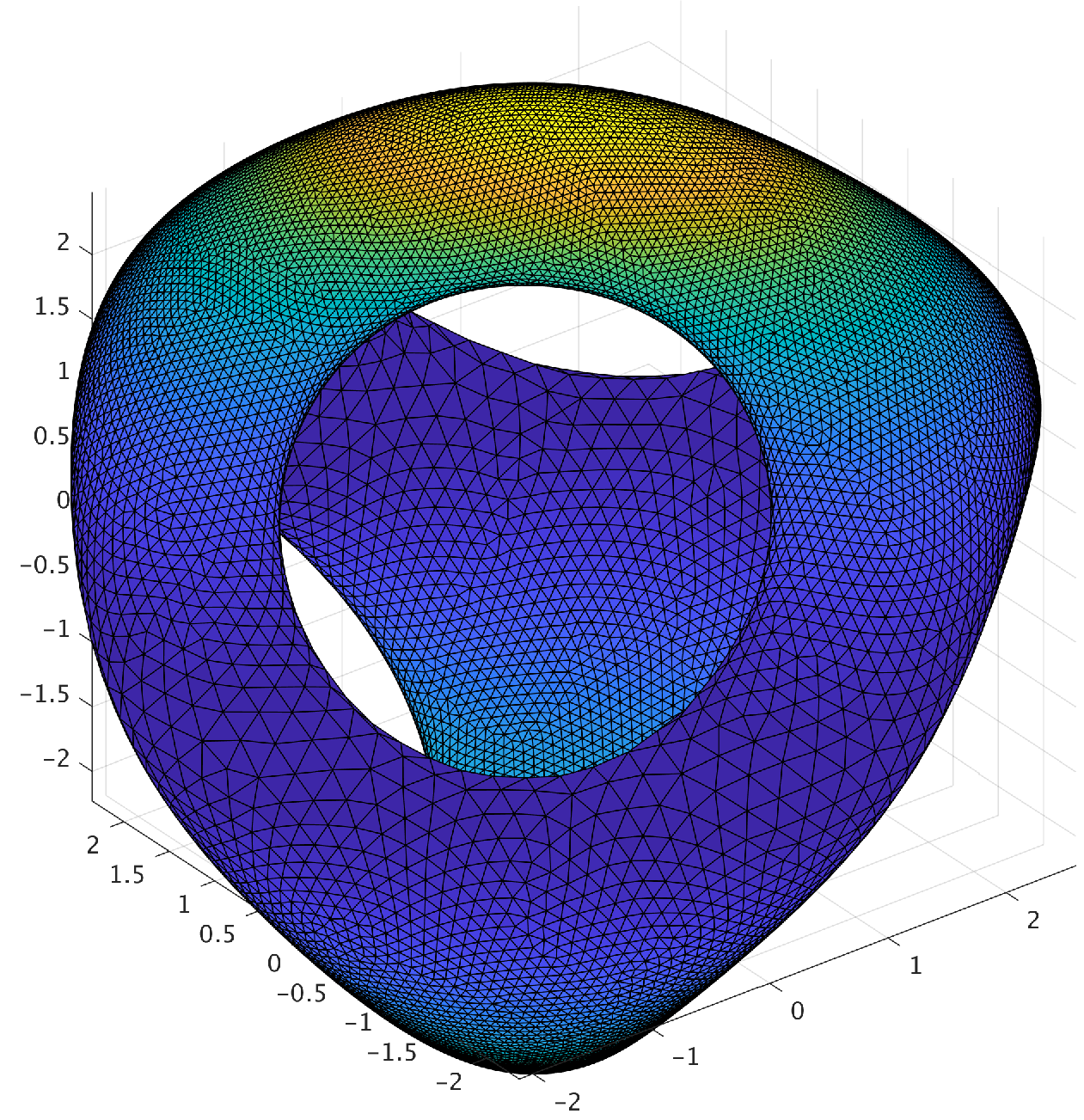
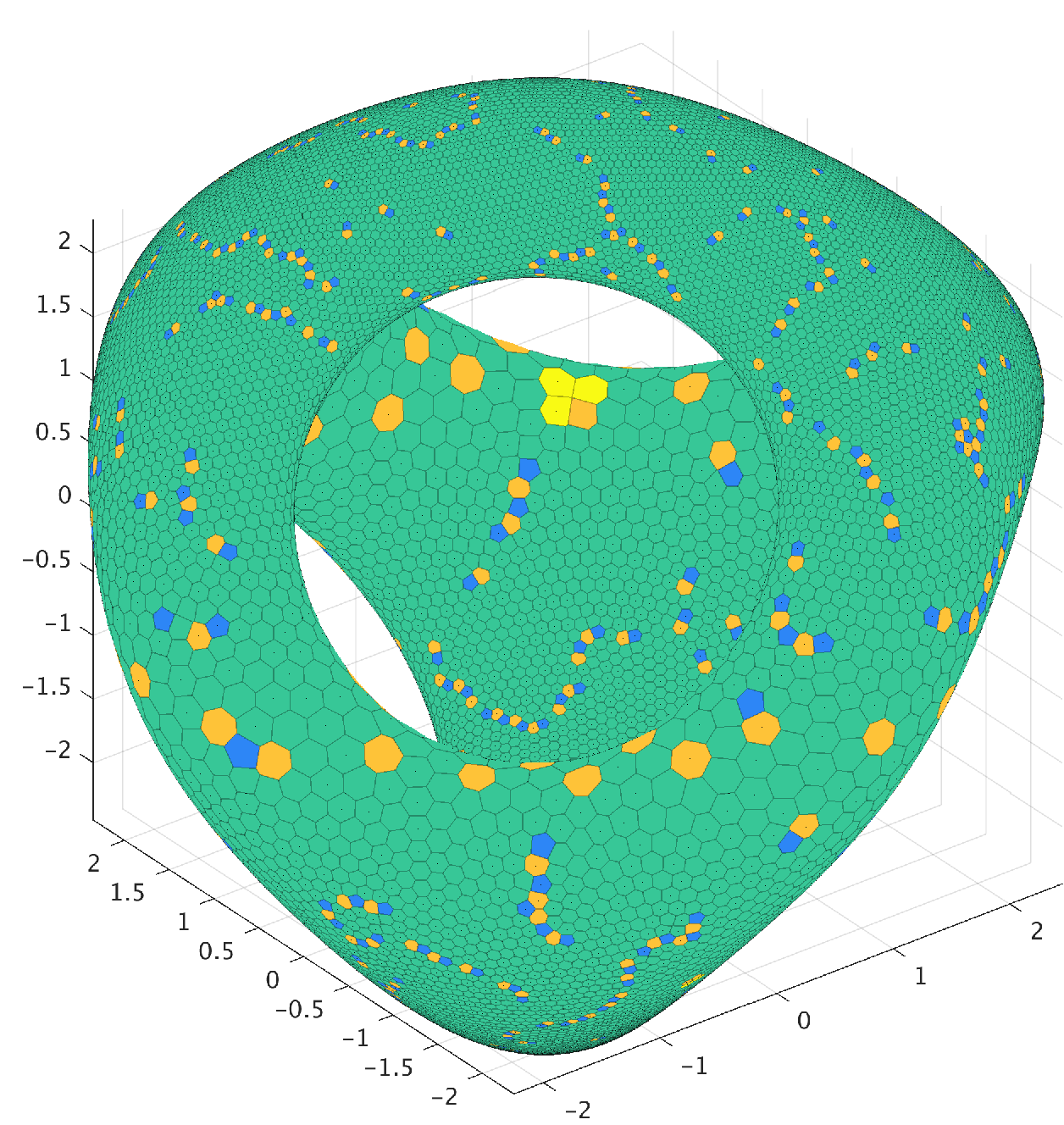
Figure 2: (Color online.) Approximate minimizing configuration of 20,000 points on a genus 3 surface in the $x_{1}x_{2}x_{3}$-cube $[-2,2]^{3}$ for the energy $E^{k}_{s}$ with $s=4$, $k=30$ and weight $w$ chosen to give density $\rho$ proportional to $x_{3}^{2}$. External field $V\equiv 0$. Left: Delaunay triangulation; right: Voronoi tessellation.

The worst case complexity for constructing the $k$-nearest neighbor ($k$-nn) graph for an $N$-point configuration is $O(N\log N)$ floating point computations (FLOPS). Thus, the cost of evaluating $E_{s}^{k}$ (or its gradient) is also $O(N\log N)$ compared with $O(N^{2})$ FLOPS for the full interaction energy $E_{s}$. However, for sufficiently well-separated point configurations, the $k$-nn algorithm reduces to $O(kN)$ and thus the cost of one energy or gradient evaluation is also $O(kN)$.

An interesting question is how the choice of $k$ influences the speed of convergence of a given optimization algorithm such as gradient descent (we remark that $E_{s}^{k}$ is not differentiable when there are ties for the $k$-th nearest neighbor). This issue is not explored here, but is left for future investigations.

In Figure 1, we show approximate energy minimizers for $N=80$ points in the unit square for the full $E_{s}$ energy (left) and $E_{s}^{k}$ energy (right) with $s=1$, $k=2$, $w\equiv 1$, and $V\equiv 0$. Notice that the full kernel energy yields higher density distribution at the boundary of the square while, in accordance with Theorem 1.1, the points are more uniformly spaced when the interactions are restricted to the $k$-nearest neighbors. The two approximate minimizers were computed using Mathematica’s IPOPT interface and the built-in simulated annealing algorithm, respectively.

It has been demonstrated that the energies $E_{s}^{k}$ can be used for efficient discretization of complicated surfaces, see [28, 27]. Here we illustrate the effectiveness of the algorithm in Figure 2 which shows an approximate minimizing configuration of $N=20\,000$ points on an algebraic surface with $s=4$, $k=30$, $V\equiv 0$, and a nonuniform weight. The left image shows the Delaunay triangulation of the configuration colored according to point density, where lighter colors reflect higher density. The right image shows the Voronoi tessellation of the surface generated by the configuration. Cells of the tessellation are colored according to their number of edges. Notice that the majority of cells are hexagons (light green).

3 Geometry of nearest neighbor interactions

3.1 Proof strategy and adjacency graph of nearest neighbors

Our strategy, as put forward in [16], is to show that the unweighted functional $E_{s}^{k}$ is a so-called short-range interaction, that is, it has the following four essential properties. Note that compared to paper [16], we strengthen and simplify the formulations, as appropriate for our context.

• Monotonicity: If $A\subset B\subset\mathbb{R}^{p}$, then, by definition,

  (3.1) $$\mathcal{E}^{k}_{s}(A,N)\geqslant\mathcal{E}^{k}_{s}(B,N),\qquad N\geqslant 1.$$

• Asymptotics on cubes: For the unit cube ${q}_{d}\in\mathbb{R}^{d}$, the following limit exists and is positive and finite

  (3.2) $$C_{s,d}^{k}:=\lim_{N\to\infty}\frac{\mathcal{E}_{s}^{k}({q}_{d},N)}{N^{1+s/d}}.$$

  This fact will be established in Lemma 4.1.

• Short-range property: The energy of a sequence of configurations contained in a pair (or finite collection) of disjoint compact sets is asymptotically the sum of energies on individual sets. Suppose $A_{1},A_{2}\subset\mathbb{R}^{p}$ are disjoint compact sets. If $\{\omega_{N}\}_{1}^{\infty}$ is a sequence of $N$-point configurations in $A_{1}\cup A_{2}$ for $N\geqslant 1$, then

  (3.3) $$\lim_{N\to\infty}\frac{E_{s}^{k}(\omega_{N}\cap A_{1})+E_{s}^{k}(\omega_{N}\cap A_{2})}{E_{s}^{k}(\omega_{N})}=1.$$

  The short-range property will be obtained in Lemma 4.4.

• Stability: The minimum energy asymptotics is stable under small perturbations (in terms of Minkowski content) of the set; that is, for every compact $A\subset\mathbb{R}^{p}$ and $\varepsilon\in(0,1)$ there is some $\delta=\delta(\varepsilon,s,k,p,d,A)>0$ such that for any compact $D\subset A$ satisfying $\mathcal{M}_{d}(D)\geqslant(1-\delta)\,\mathcal{M}_{d}(A)$, we have

  (3.4) $$\liminf_{N\to\infty}\frac{\mathcal{E}^{k}_{s}(A,N)}{N^{1+s/d}}\geqslant(1-\varepsilon)\liminf_{N\to\infty}\frac{\mathcal{E}^{k}_{s}(D,N)}{N^{1+s/d}},\quad\limsup_{N\to\infty}\frac{\mathcal{E}^{k}_{s}(A,N)}{N^{1+s/d}}\geqslant(1-\varepsilon)\limsup_{N\to\infty}\frac{\mathcal{E}^{k}_{s}(D,N)}{N^{1+s/d}}.$$

  In addition, for $p=d$, $\delta$ is independent of $A$. This result will be established in Lemma 4.5.

Once these properties have been established for the unweighted interaction $E_{s}^{k}$, existence of the asymptotics on compact sets in $\mathbb{R}^{d}$ follows as an extension of the statement (ii) for cubes. The statement of Theorem 1.1, applying to $({\mathcal{H}}_{d},d)$-rectifiable sets $A\subset\mathbb{R}^{p}$ with $\mathcal{H}_{d}(A)=\mathcal{M}_{d}(A)$, is then derived by approximating such sets with bi-Lipschitz parametrizations, an argument going back to Federer [10].

For some of the proofs in the sequel it will be useful to order the entries of $\omega_{N}\in(\mathbb{R}^{p})^{N}$ by their distance to a given $x\in\mathbb{R}^{p}$; as was mentioned in Section 1, the interaction $E_{s}^{k}$ selects points with smaller indices in the case of equal distance, so we will order lexicographically, first by distance, then by index. Formally, the order $\prec_{x}$ on entries of $\omega_{N}$ is defined like so:

$$y\prec_{x}z\qquad\stackrel{{\scriptstyle def}}{{\iff}}\qquad\begin{aligned} \|y-x\|&<\|z-x\|\\ \text{ or }\\ \|y-x\|&=\|z-x\|\text{ and }I(y;\omega_{N})<I(z;\omega_{N}),\end{aligned}$$

where as before, $I(y;\omega_{N})$ is the index of the first occurrence of $y$ as an entry of $\omega_{N}$. The notation $\mathcal{N}_{k}(x;\omega_{N})$ introduced above then stands for the tuple of the first $k$ entries of $\omega_{N}\setminus\{x\}$ with respect to the ordering $\prec_{x}$. We further write $(x;\omega_{N})_{l}$ for the $l$-th entry of $\omega_{N}\setminus\{x\}$ with respect to $\prec_{x}$, $1\leqslant l\leqslant N-1$. In particular, distances $\|x-(x;\omega_{N})_{l}\|$ are nondecreasing in $l$ for a fixed $x$ and $\omega_{N}$.

Let

$$\Lambda_{k}(\omega_{N}):=\{(x,y):x,y\in\omega_{N},\ y\in\mathcal{N}_{k}(x;\omega_{N})\},$$

the set of ordered pairs of entries of $\omega_{N}$, corresponding to the relation “$y$ is among the $k$ nearest neighbors of $x$”. Notice that this relation is not symmetric. In what follows, it will be occasionally convenient to think of $\Lambda_{k}(\omega_{N})$ as the set of edges in the oriented graph $(\mathcal{V},\mathcal{E})=\left(\{x_{i}\}_{1}^{N},\ \Lambda_{k}(\omega_{N})\right)$ with $\{x_{i}\}_{1}^{N}$ being the multiset of entries from $\omega_{N}$. Due to this, we will refer to $\Lambda_{k}$ as the adjacency graph of $\omega_{N}$.

3.2 Main geometric lemma and local properties of near-minimizers

Using $\Lambda_{k}(\omega_{N})$, we can write

(3.5) $$E^{k}_{s}(\omega_{N};w,V)=\sum_{(x,y)\in\Lambda_{k}(\omega_{N})}w(x,y)\|x-y\|^{-s}+N^{s/d}\sum_{x\in\omega_{N}}V(x),\qquad s\neq 0.$$

As before, the function $w$ is assumed to be a CPD-weight on $A\times A$. The external field $V$ is assumed to be lower semicontinuous on $A$ (and therefore bounded below there).

Our eventual goal is to verify the properties from Section 3.1. It is easy to see that restricting interactions to $k$ nearest neighbors guarantees that $E^{k}_{s}$ is in a sense local. Without such restriction, the locality does not hold when $s<d$, as is well-known from classical potential theory. Since $s>0$, the singular nature of the interaction on the diagonal results in that the pointwise separation is of the optimal order for near-minimizers, as will be shown in Theorem 1.3.

We will first obtain the following basic fact about the set $\Lambda_{k}(\omega_{N})$.

Lemma 3.1.

Fix a configuration $\omega_{N}\in(\mathbb{R}^{d})^{N}$ of $N$ distinct points. For any $y\in\omega_{N}$, the number of points $x$ in $\omega_{N}$ such that $y$ is one of $k$ nearest neighbors of $x$ is bounded by $n(k,d)$, depending only on the number of neighbors $k$ and the dimension $d$. That is,

$$\#\{x\in\omega_{N}:y\in\mathcal{N}_{k}(x;\omega_{N})\}\leqslant n(k,d).$$

This lemma can be interpreted in graph-theoretic terms as follows. Consider expression (3.5); the first sum involves terms $w(x,y)\|x-y\|^{-s}$ for oriented pairs $(x,y)\in\Lambda_{k}(\omega_{N})$. By definition, the outgoing degree of every vertex in the graph $\left(\{x_{i}\}_{1}^{N},\ \Lambda_{k}(\omega_{N})\right)$ is $k$; the above lemma shows further that the maximal incoming degree in the graph is bounded by $n(k,d)$. It is also useful to note that $y$ does not have to be an element of $\omega_{N}$ for the result to hold.

• Fix $y\in\omega_{N}$ and denote $\omega_{N,y}=\{x\in\omega_{N}:y\in\mathcal{N}_{k}(x;\omega_{N})\}$. Choose the radius $r_{y}>0$ so that $B(y,r_{y})$ does not contain any points from $\omega_{N}$ except $y$. Let $\pi_{S}$ be the radial projection onto the sphere $S:=\partial B(y,r_{y})$ and consider the image $\pi_{S}(\omega_{N,y})$, see Figure 3.

  Figure 3: The open spherical cap of radius $\pi/3$ around projection $\pi_{S}(x_{i})$ (dashed) contains the projection of $x_{i^{\prime}}$. As Lemma 3.1 shows, at most $k$ points among $\{x\in\omega_{N}:y\in\mathcal{N}_{k}(x;\omega_{N})\}$ can be projected into any given cap of angular radius $\pi/6$ (shaded).

  Suppose that an open spherical cap $B_{S}(z,\pi/6)$ on $S$ of angular radius $\pi/6$ and center $z\in S$ contains more than $k$ elements of this image. Let

  $$x_{i}=\arg\max\{\|x-y\|:x\in\omega_{N,y},\ \pi_{S}(x)\in B_{S}(z,\pi/6)\}.$$

  Then $B_{S}(z,\pi/6)\subset B_{S}(\pi_{S}(x_{i}),\pi/3)$, implying for any $x_{i^{\prime}}\in\omega_{N,y}$, from $\pi_{S}(x_{i^{\prime}})\in B_{S}(z,\pi/6)$ it follows $\angle x_{i}yx_{i^{\prime}}<\pi/3$, so that

  $$\|x_{i^{\prime}}-x_{i}\|<\max\{\|y-x_{i}\|,\|y-x_{i^{\prime}}\|\}=\|y-x_{i}\|,$$

  since $x_{i}$ was chosen the furthest from $y$. Thus, every other point projected into $B_{S}(\pi_{S}(z),\pi/6)$ is closer to $x_{i}$ than $y$, and it must be $y\notin\mathcal{N}_{k}(x_{i};\omega_{N})$, a contradiction. By this argument, the constant $n(k,d)$ chosen as

  $$n(k,d):=\max\left\{n:\exists\,\omega_{n}\in(\mathbb{S}^{d-1})^{n}\text{ such that }\#(\omega_{n}\cap B_{S}(z,\pi/6))\leqslant k,\ \forall z\in\mathbb{S}^{d-1}\right\}$$

  has the properties stated in the claim of the lemma. ∎

We will also need a classical result from potential theory, due to Frostman.

Proposition 3.2 (Frostman’s lemma [23, p. 112], [12]).

For any compact $A\subset\mathbb{R}^{p}$ with $\mathcal{H}_{d}(A)>0$, there is a finite nontrivial Borel measure $\mu$ on $\mathbb{R}^{p}$ with support inside $A$ such that

$$\mu(B(x,r))\leqslant r^{d},\qquad{x}\in\mathbb{R}^{p},\ r>0.$$

This statement is used to obtain a lower bound on the optimal covering radius of the compact set $A$. Indeed, let the measure $\mu$ be as in Frostman’s lemma. Given any collection $\omega_{N}=(x_{i})_{1}^{N}\in A^{N}$, for the radius $r_{0}=c_{{}_{\rm Fro}}(A)N^{-1/d}:=(\mu(A)/2)^{1/d}N^{-1/d}$ and the set

$$D=A\setminus\bigcup_{i}B({x}_{i},r_{0})$$

there holds $\mu(D)\geqslant\mu(A)/2$. In particular $D\neq\emptyset$, so that at least one point of $A$ is distance $r_{0}$ away from the points in $\omega_{N}$. It follows that the covering radius of $A$ for any collection of $N$ points $\omega_{N}\in A^{N}$ is at least $c_{{}_{\rm Fro}}(A)N^{-1/d}$. Observe also that for $d=p$, it suffices to use $\mu=v_{d}^{-1}\mathcal{L}_{d}$, and hence $\mu$ is independent of $A$ in this case.

• Fix an $N>2$. Since $s>0$ and the product $w(x,y)\|x-y\|^{-s}$ is infinite on the diagonal of $A\times A$, assumptions of the theorem imply that all entries of $\omega_{N}$ are distinct. It will be convenient to assume that configuration $\omega_{N}=(x_{1},\ldots,x_{N})$ is numbered in such a way that minimal separation is attained for the pair $x_{1},x_{2}$:

  $$\Delta(\omega_{N})=\|x_{1}-x_{2}\|=c_{N}N^{-1/d}.$$

  It will also be convenient to assume $V\geqslant 0$ on $A$; by lower semicontinuity this can be achieved by adding a sufficiently large constant to $V$, which does not change the behavior of minimizers.

  We need to show $c_{N}\geqslant C(s,k,d,w,V,A,R)>0$, $N\geqslant 1$. By definition, a PD-weight satisfies properties (b)-(c) of a CPD-weight; thus there exists a $\delta>0$ such that $\{(x,z):\|x-z\|\leqslant\delta\}\subset G$ for the neighborhood $G$ as in the definition of CPD-weight. This implies

  $$0<m_{w}:=\inf\{w(x,z):\|x-z\|\leqslant\delta\}.$$

  Let further $M_{w}$ be as in (1.7) and $L=\sup_{D}V$ – both finite quantities, due to the boundedness of $w$ and $V$ on $D$.

  Since $D$ is a set of positive $\mathcal{H}_{d}$-measure, and in view of the discussion after Proposition 3.2, there exists a point $z\in D$, such that

  $$\|z-x_{i}\|\geqslant c_{{}_{\rm Fro}}N^{-1/d},\qquad i=1,\ldots,N,$$

  where $c_{{}_{\rm Fro}}:=c(D)=(\mu(D)/2)^{1/d}$ is from Frostman’s lemma for $D$. Let

  $$\omega_{N}^{\prime}=(z,x_{2},\ldots,x_{N}),$$

  the configuration obtained by replacing $x_{1}$ with $z$. If $\|x_{1}-x_{2}\|=c_{N}N^{-1/d}\geqslant\delta$, there is nothing to prove. Otherwise, suppose $c_{N}N^{-1/\,{d}}<\delta$ for some $N$. Since $E^{k}_{s}(\omega_{N};w)$ is close to being optimal, replacing $x_{1}$ with $z$ can lower the value of $E_{s}^{k}$ by at most $RN^{s/d}$:

  $$E^{k}_{s}(\omega_{N}^{\prime};w,V)-E^{k}_{s}(\omega_{N};w,V)=E^{k}_{s}(\omega_{N}^{\prime};w)-E^{k}_{s}(\omega_{N};w)+N^{s/d}(V(z)-V(x_{1}))\geqslant-RN^{s/d},$$

  so that, since $V(z)-V(x_{1})\leqslant V(z)\leqslant L$,

  (3.6) $$E^{k}_{s}(\omega_{N}^{\prime};w)-E^{k}_{s}(\omega_{N};w)\geqslant-(R+L)N^{s/d}.$$

  Let us determine the terms remaining after cancellation in the left-hand side of this equation. Since

  $$E^{k}_{s}(\omega_{N}^{\prime};w)-E^{k}_{s}(\omega_{N};w)=\left(\sum_{(x,y)\in\Lambda_{k}(\omega_{N}^{\prime})}-\sum_{(x,y)\in\Lambda_{k}(\omega_{N})}\right)w(x,y)\|x-y\|^{-s},$$

  we can describe all the terms that occur only in $E_{s}^{k}(\omega_{N};w)$, and therefore do not cancel out, as

  $$\Sigma_{1}+\Sigma_{2}+\Sigma_{3}:=\left(\sum\limits_{\begin{subarray}{c}(x,y)\in\Lambda_{k}(\omega_{N}),\\ x=x_{1}\end{subarray}}+\sum\limits_{\begin{subarray}{c}(x,y)\in\Lambda_{k}(\omega_{N}),\\ y=x_{1}\end{subarray}}+\sum\limits_{\begin{subarray}{c}(x,y)\in\Lambda_{k}(\omega_{N})\setminus\Lambda_{k}(\omega_{N}^{\prime})\\ x,y\neq x_{1}\end{subarray}}\right)w(x,y)\|x-y\|^{-s}.$$

  Likewise, the terms occurring only in $E_{s}^{k}(\omega_{N}^{\prime};w)$ are as follows:

  $$\Sigma_{4}+\Sigma_{5}+\Sigma_{6}:=\left(\sum\limits_{\begin{subarray}{c}(x,y)\in\Lambda_{k}(\omega_{N}^{\prime}),\\ x=z\end{subarray}}+\sum\limits_{\begin{subarray}{c}(x,y)\in\Lambda_{k}(\omega_{N}^{\prime}),\\ y=z\end{subarray}}+\sum\limits_{\begin{subarray}{c}(x,y)\in\Lambda_{k}(\omega_{N}^{\prime})\setminus\Lambda_{k}(\omega_{N})\\ x,y\neq z\end{subarray}}\right)w(x,y)\|x-y\|^{-s}.$$

  The term $\sum_{3}$ above arises due to the number of terms originating from each point being fixed at $k$, so any terms incoming into $z$ must have had different terminating nodes in $\omega_{N}$; similar logic applies to $\sum_{6}$.

  Figure 4: Elements of $\Lambda_{1}(\omega_{5})$ compared to those in $\Lambda_{1}(\omega_{5}^{\prime})$. Arrow from node $x$ to node $y$ means that pair $(x,y)$ is present in the respective adjacency graph. Solid arrows show pairs present in both graphs; wavy arrows represent pairs appearing only in $\Lambda_{1}(\omega_{5}^{\prime})$; dashed arrows those appearing only in $\Lambda_{1}(\omega_{5})$. For this small example, each of $\Sigma_{m}$ contains exactly one term/edge.

  To summarize, there holds

  $$E^{k}_{s}(\omega_{N}^{\prime};w)-E^{k}_{s}(\omega_{N};w)=\Sigma_{4}+\Sigma_{5}+\Sigma_{6}-\Sigma_{1}-\Sigma_{2}-\Sigma_{3}.$$

  As an illustration, all the six sums $\Sigma_{m}$ are present when point $x_{1}$ is replaced with $z$ in the tuple $\omega_{5}=(x_{i})_{1}^{5}$, shown in Figure 4. In this figure, ordered pairs $(x,y)\in\Lambda_{1}$ for either tuple are represented as directed edges of a graph.

  To finish the proof, we will need an upper bound on $\Sigma_{6}-\Sigma_{2}$. To that end, note that each pair in $\Sigma_{6}$, that is,

  $$(x,y)\in\Lambda_{k}(\omega_{N}^{\prime})\setminus\Lambda_{k}(\omega_{N})\quad\text{such that }x,y\neq z,$$

  must be replacing a pair having the form $(x,x_{1})$ in $\Lambda_{k}(\omega_{N})$, to keep the total number of outgoing edges from $x$ equal to $k$. Grouping the new pairs in $\Sigma_{6}$ with the removed ones in $\Sigma_{2}$ by their starting node gives

  $$\Sigma_{6}-\Sigma_{2}=\sum_{\begin{subarray}{c}x:\ (x,x_{1})\in\Lambda_{k}(\omega_{N}),\\ z\notin\mathcal{N}_{k}(x;\,\omega_{N}^{\prime})\end{subarray}}\left(\frac{w(x,(x;\omega_{N})_{k+1})}{\|x-(x;\omega_{N})_{k+1}\|^{s}}-\frac{w(x,x_{1})}{\|x-x_{1}\|^{s}}\right)\leqslant 0,$$

  since $\|x-x_{1}\|\leqslant\|x-(x;\omega_{N})_{k+1}\|$, and $w$ is marginally radial, so the expression $w(x,y)/\|x-y\|^{-s}$ is nonincreasing with the distance $\|x-y\|$ for every fixed $x$. We used the notation $(x,\omega_{N})_{k+1}$ for the $(k+1)$-st nearest neighbor to $x$ in $\omega_{N}$, as introduced in Section 3.1. Finally, equation (3.6) implies

  $$-(R+L)N^{s/d} \leqslant\Sigma_{4}+\Sigma_{5}+\Sigma_{6}-\Sigma_{1}-\Sigma_{2}-\Sigma_{3}$$

  $$\leqslant\Sigma_{4}+\Sigma_{5}+(\Sigma_{6}-\Sigma_{2})-\Sigma_{1}$$

  $$\leqslant\sum_{x\in\mathcal{N}_{k}(z;\omega_{N}^{\prime})}\frac{w(z,x)}{\|z-x\|^{s}}+\sum_{x:z\in\mathcal{N}_{k}(x;\omega_{N}^{\prime})}\frac{w(x,z)}{\|x-z\|^{s}}-\frac{w(x_{1},x_{2})}{\|x_{1}-x_{2}\|^{s}}$$

  $$\leqslant\left(kM_{w}c_{{}_{\rm Fro}}^{-s}+n(k,p)M_{w}c_{{}_{\rm Fro}}^{-s}-m_{w}c_{N}^{-s}\right)N^{s/d},$$

  where in the fourth inequality Lemma 3.1 is used to estimate the number of terms in the second sum.

  This implies that whenever $c_{N}<\delta N^{1/d}$, there holds

  (3.7) $$c_{N}\geqslant\left(\frac{m_{w}}{(R+L)\,c_{{}_{\rm Fro}}^{s}+(k+n(k,p))M_{w}}\right)^{1/s}c_{{}_{\rm Fro}},$$

  as desired. ∎

Corollary 3.3.

Let $w\equiv 1$ and $p=d$; let also $\omega_{N}^{*}$ be such that $E_{s}^{k}(\omega_{N}^{*})\leqslant\mathcal{E}_{s}^{k}(A,N)+1$. Then equation (3.7) implies

$$\Delta(\omega_{N}^{*})\geqslant\left(\frac{1}{1+k+n(k,d)}\right)^{1/s}c_{{}_{\rm Fro}}\,N^{-1/d},\qquad N\geqslant N_{0}(d,\mathcal{L}_{d}(A)),$$

where $c_{{}_{\rm Fro}}=c(d)\mathcal{L}_{d}(A)^{1/d}$, as in the discussion after Proposition 3.2.

• It suffices to note that under such assumptions on $\omega_{N}^{*}$, $L=0$, $R\leqslant N^{-s/d}$, and $m_{w}=M_{w}$ = 1 in equation (3.7). ∎

Corollary 3.4.

The proof of Theorem 1.3 shows that there holds an optimal covering result, at least for some sublevel set of $V+w$. In particular, when $V\equiv 0$, $w\equiv 1$ one has an optimal covering result: For a compact set $A\subset\mathbb{R}^{d}$ with $0<\mathcal{\mathcal{H}}_{d}(A)<\infty$, and a sequence of configurations $\{\omega_{N}^{*}\}_{1}^{\infty}$, such that

$$E_{s}^{k}(\omega_{N})\leqslant\mathcal{E}_{s}^{k}(A,N)+RN^{s/d},\qquad N\geqslant 1,$$

for every $y\in A$ there holds

$$\operatorname*{dist}(y,\omega_{N})\leqslant C(s,k,d,A,R)\,N^{-1/d}.$$

• It suffices to note that in the proof of the theorem, one obtains the inequality (3.7) between the covering radius at $z\in D$, equal to $c_{{}_{\rm Fro}}N^{-1/d}$, and the minimal separation, equal to $c_{N}N^{-1/d}$. Using $\mathcal{H}_{d}(A)<\infty$ and a standard volume argument, one easily obtains an upper bound of $C(A)N^{-1/d}$ on the optimal separation, at least for $p=d$. In the case $p>d$, one uses instead the finiteness of the Minkowski content, $\mathcal{M}_{d}(A)<\infty$, to the same effect. In the sequel, we shall only need the optimal covering property for the unit cube in $\mathbb{R}^{d}$ in Section 4.1. It is not hard to see that the optimal covering holds on the $L_{1}$-sublevel set for $V$, with $L_{1}$ from the statement of Theorem 1.1, and is not guaranteed on any larger sublevel set. ∎

Existence of minimizers of $E^{k}_{s}$ The above theorem concerns configurations with near-optimal value of energy. A natural question to ask is, under which assumptions on $w$ the functional (3.5) attains its minimum on $A^{N}$; that is, whether $E^{k}_{s}$ is lower semicontinuous. Recall that the topology on $A^{N}$ is the product topology induced by the restriction of Euclidean metric to $A$. In the following proof it will be convenient to use $l^{\infty}$ norm on $A^{N}$, so that distance between two configurations is

$$\rho(\omega_{N}^{\prime},\omega_{N}^{\prime\prime})=\max_{i}\|x_{i}^{\prime}-x_{i}^{\prime\prime}\|.$$

Lemma 3.5.

Let $V$ be lower semicontinuous on $A$. If $w$ is a weight of the form

$$w(x,y)=W(x,\|x-y\|),$$

with $W$ lower semicontinuous on $A\times[0,\text{\rm diam}(A)]$, then $E^{k}_{s}(\omega_{N};w,V)$ is lower semicontinuous on $A^{N}$ for any fixed $N\geqslant 1$.

Remark 3.6.

To see that $w$ must indeed only depend on the distance $\|x-y\|$, let $d=2$ and

$$\omega_{3}^{(n)}=(x_{1},x_{2}^{(n)},x_{3})=\left((0,0),\ \left(0,1+2^{-n}\right),\ (1,0)\right)$$

be a sequence of 3-point configurations, converging to $\omega_{3}=(x_{i})_{1}^{3}:=\left((0,0),\ (0,1),\ (1,0)\right)$. Let further $w$ be continuous, symmetric, and such that

$$w((0,0),\ (0,1))=3,\qquad w((0,0),\ (1,0))=1.$$

Then

$$E_{1}^{1}(\omega_{3}^{(n)})=3\|x_{2}^{(n)}\|^{-1}+2\|x_{3}\|^{-1}\to 5,\quad n\to\infty,$$

while

$$E_{1}^{1}(\omega_{3})=2\cdot 3\|x_{2}\|^{-1}+\|x_{3}\|^{-1}=7,$$

since the tie-breaking convention in $E_{1}^{1}$ prefers points with smaller indices (see page 1.1), thereby violating the lower semicontinuity.

• Fix a configuration $\omega_{N}^{\circ}=\{x_{1}^{\circ},\ldots,x_{N}^{\circ}\}$. In this proof, points and indices related to $\omega_{N}^{\circ}$ will be denoted by the ^∘ superscript. Objects related to a variable configuration $\omega_{N}$, approaching $\omega_{N}^{\circ}$ in the product topology, will not carry this superscript.

  If $x_{i}^{\circ}=x_{j}^{\circ}$ for some $i\neq j$, $E^{k}_{s}(\omega_{N}^{\circ};w,V)=+\infty$. Due to the lower semicontinuity and nonnegativity of $\|\cdot\|^{-s}$ and $w$, and lower semicontinuity of $V$, there holds

  $$E^{k}_{s}(\omega_{N};w,V)\to+\infty,\qquad\hbox{ whenever }\omega_{N}\to\omega_{N}^{\circ}\text{ in }A^{N}.$$

  Let now $\omega_{N}^{\circ}$ consist of distinct points and $V\equiv 0$. Fix an $\varepsilon>0$. Note that when $\omega_{N}=\{x_{i}\}_{1}^{N}$ is sufficiently close to $\omega_{N}^{\circ}$ in the $l^{\infty}$ metric on $A^{N}$, so that for $\Delta$ as in (1.6),

  $$\|x_{i}-x_{i}^{\circ}\|<\Delta(\omega_{N}^{\circ})/3,\qquad 1\leqslant i\leqslant N,$$

  then the value of $E_{s}^{k}(\omega_{N})$ continuously depends on $x_{i}$. In addition, by lower semicontinuity of $w$, for a sufficiently small $\delta_{1}=\delta(\varepsilon)$, one has

  $$w(x_{i},x_{j})\|x_{i}-x_{j}\|^{-s}\geqslant w(x_{i}^{\circ},x_{j}^{\circ})\|x_{i}^{\circ}-x_{j}^{\circ}\|^{-s}-\frac{\varepsilon}{k}$$

  whenever $r_{ij}:=\|x_{i}-x_{j}\|$ and $r_{ij}^{\circ}:=\|x_{i}^{\circ}-x_{j}^{\circ}\|$ differ by at most $\delta_{1}$ for $1\leqslant i,j\leqslant N$ (we used here the specific form of $w$).

  We shall further need to show that the nearest neighbor structure $\Lambda_{k}(\omega_{N})$ does not change much in a neighborhood of $\omega_{N}^{\circ}$ – or more precisely, distances to the $k$ nearest neighbors remain approximately the same, even if the points themselves may be different. Fix an index $i$. To obtain lower semicontinuity of $E_{s}^{k}(\omega_{N};w)$, it suffices to verify the semicontinuity at $\omega_{N}^{\circ}$ only for the sum

  $$\sum_{x_{j}\in\mathcal{N}_{k}(x_{i};\omega_{N})}\|x_{i}-x_{j}\|^{-s}$$

  as a function of configuration $\omega_{N}$. Consider distances from $x_{i}^{\circ}$ to the other entries of $\omega_{N}^{\circ}$:

  $$d_{l}:=\|x_{i}^{\circ}-(x_{i}^{\circ};\omega_{N}^{\circ})_{l}\|,\qquad 1\leqslant l\leqslant N.$$

  By the definition of $(x_{i}^{\circ};\omega_{N}^{\circ})_{l}$, $d_{l+1}\geqslant d_{l}$. Let $\{D_{l}\}_{1}^{K}$ be the strictly increasing sequence of unique values among $\{d_{l}\}$, $K\leqslant N$. Partition the multiset of entries of $\omega_{N}^{\circ}$ as

  $$\bigsqcup_{l=1}^{K}J^{\circ}_{l},\qquad J_{l}^{\circ}:=\{y\in\omega_{N}^{\circ}:\|x_{i}^{\circ}-y\|=D_{l}\},$$

  according to the unique distances to $x_{i}^{\circ}$. Note that when a configuration $\omega_{N}=(x_{1},\ldots,x_{N})\in A^{N}$ is such that $\|x_{j}-x_{j}^{\circ}\|<\delta$, $1\leqslant j\leqslant N$, with

  $$\delta<\min\left[\delta_{1},\ \min\left\{(D_{l+1}-D_{l})/4\right\}_{1}^{K-1}\right],$$

  there holds

  $$\|x_{i}-x_{j_{1}}\|<\|x_{i}-x_{j_{2}}\|,\qquad x_{j_{1}}^{\circ}\in J_{l_{1}}^{\circ},\ x_{j_{2}}^{\circ}\in J_{l_{2}}^{\circ},\ l_{1}<l_{2}.$$

  That is, the entries of $\omega_{N}\setminus\{x_{i}\}$ can be collected into $K$ groups, $\{J_{l}\}_{1}^{K}$, with any element of a group $J_{l_{1}}$ closer to $x_{i}$ than any element of another group $J_{l_{2}}$ when $l_{1}<l_{2}$. By construction,

  $$\#J_{l}^{\circ}=\#J_{l},\qquad 1\leqslant l\leqslant K,$$

  so there is a bijection between elements of corresponding groups. Observe also that for every pair of elements $y,z\in J_{l}$ and a pair $y^{\circ},z^{\circ}\in J_{l}^{\circ}$, belonging to corresponding groups, there holds

  $$\big{|}\,|\|y-z\|-\|y^{\circ}-z^{\circ}\|\,\big{|}<2\delta,$$

  which by the definition of $\delta_{1}$ gives

  $$w(y,z)\|y-z\|^{-s}\geqslant w(y^{\circ},z^{\circ})\|y^{\circ}-z^{\circ}\|^{-s}-\frac{\varepsilon}{k}.$$

  By the aforementioned bijection between groups $J_{l}^{\circ}$ and $J_{l}$, this implies

  $$\sum_{x_{j}\in\mathcal{N}_{k}(x_{i};\omega_{N})}w(x_{i},x_{j})\|x_{i}-x_{j}\|^{-s}\geqslant\sum_{x_{j}\in\mathcal{N}_{k}(x_{i}^{\circ};\omega_{N}^{\circ})}w(x_{i}^{\circ},x_{j}^{\circ})\|x_{i}^{\circ}-x_{j}^{\circ}\|^{-s}-{\varepsilon},$$

  proving the lower semicontinuity of the point energy for a single $x_{i}$, and therefore lower semicontinuity of $E_{s}^{k}(\cdot\,;w)=E_{s}^{k}(\cdot\,;w,0)$. Addition of an external field is only introducing another lower semicontinuous term, which completes the proof. ∎

Corollary 3.7.

Under the assumptions of Lemma 3.5, minimizing the $k$-energy for any $k\geqslant 1$ and $s>0$ yields a separated configuration.

4 Proofs of the main results

4.1 Asymptotics on cubes

Let us demonstrate the existence of asymptotics on cubes for the Riesz $k$-energy functionals, following the outline in Section 3.1. We shall need this fact only for the unweighted $E_{s}^{k}$ – or, equivalently, for the constant weight $w$ and zero external field $V$. In this section, the ambient space is $\mathbb{R}^{d}$.

Lemma 4.1.

For $s>0$ and $k,d$ positive integers, the following limit exists, and is positive and finite:

(4.1) $$C_{s,d}^{k}:=\lim_{N\to\infty}\,\frac{\mathcal{E}_{s}^{k}({q}_{d},N)}{N^{1+s/d}},$$

which is the constant appearing in (1.5).

• Set

  $$\underline{\textswab{L}}:=\liminf_{N\to\infty}\frac{\mathcal{E}_{s}^{k}({q}_{d},N)}{N^{1+s/d}}.$$

  Fix $\varepsilon>0$ and let $\{\underline{\omega}_{n}\}_{n\in\underline{\mathscr{N}\mkern-6.0mu}\mkern 6.0mu}$ be a subsequence of $n$-point configurations in ${q}_{d}$ for which

  $$E_{s}^{k}(\underline{\omega}_{n})<(\underline{\textswab{L}}+\varepsilon)n^{1+s/d},\qquad n\in\underline{\mathscr{N}\mkern-6.0mu}\mkern 6.0mu.$$

  We shall show that

  $$\overline{\textswab}{L}:=\limsup_{N\to\infty}\frac{\mathcal{E}_{s}^{k}({q}_{d},N)}{N^{1+s/d}},$$

  equals $\underline{\textswab{L}}$, establishing the existence of the limit (4.1).

For any $N\geqslant 1$, let $\{\overline{\omega}_{N}\}$ be an $N$-point configuration in ${q}_{d}$ such that

(4.2) $$E_{s}^{k}(\overline{\omega}_{N})<\mathcal{E}_{s}^{k}({q}_{d},N)+1.$$

Let $n\in\underline{\mathscr{N}\mkern-6.0mu}\mkern 6.0mu$ and $L$ be the unique positive integer such that

(4.3) $$n(L-1)^{d}\leqslant N<nL^{d}.$$

By Corollary 3.4, there is a positive constant $c(s,k,d)$ such that the distance to the $k$-th nearest neighbor in $\underline{\omega}_{n}$ is at most $c(s,k,d)n^{-1/d}$. Let

$$\gamma:=1-c(s,k,d)n^{-1/d},$$

and consider the following configuration obtained by tiling ${q}_{d}$ with copies of $\gamma\underline{\omega}_{n}/L$:

$$\omega:=\bigcup_{\boldsymbol{i}\in\,(L\mathbb{Z})^{d}}\left(\frac{\gamma}{L}\underline{\omega}_{n}+\frac{\boldsymbol{i}}{L}\right),$$

where $L\mathbb{Z}:=\{0,1,\ldots,L-1\}$. We observe that with this choice of $\gamma$ the $k$ nearest neighbors in $\omega$ for every point in the subset $\frac{\gamma}{L}\underline{\omega}_{n}+\frac{\boldsymbol{i}}{L}$ also belong to this subset.

We next obtain an upper bound for $E_{s}^{k}(\overline{\omega}_{N})$ using $\omega$. By the scale invariance of $E_{s}^{k}$ there holds

$$E_{s}^{k}\left(\frac{\gamma}{L}\underline{\omega}_{n}\right)=\left(\frac{L}{\gamma}\right)^{s}E_{s}^{k}(\underline{\omega}_{n}),$$

and so from (4.2) and (4.3), we have

(4.4) $$\frac{E_{s}^{k}(\overline{\omega}_{N})}{N^{1+s/d}} \leqslant\frac{E_{s}^{k}(\omega)+1}{N^{1+s/d}}=\frac{L^{d}\,\left(\frac{L}{\gamma}\right)^{s}E_{s}^{k}(\underline{\omega}_{n})+1}{N^{1+s/d}}$$

$$\leqslant\frac{L^{d}\,\left(\frac{L}{\gamma}\right)^{s}E_{s}^{k}(\underline{\omega}_{n})}{(n(L-1)^{d})^{1+s/d}}+N^{-1-s/d}$$

$$\leqslant\gamma^{-s}\left(\frac{L}{L-1}\right)^{s+d}(\underline{\textswab{L}}+\varepsilon)+N^{-1-s/d},$$

where in the first equality we used that due to the choice of $\gamma$, no interactions between different tiles enter the sum for $E_{s}^{k}(\omega)$. Taking the limit superior as $N\to\infty$ in (4.4) for fixed $n$ which implies $L\to\infty$, gives

$$\overline{\textswab}{L}\leqslant\gamma^{-s}(\underline{\textswab{L}}+\varepsilon).$$

Then taking $n\to\infty$, $n\in\underline{\mathscr{N}\mkern-6.0mu}\mkern 6.0mu$, (in which case $\gamma\to 1$) shows that $\overline{\textswab}{L}\leqslant\underline{\textswab{L}}+\varepsilon.$ Since $\varepsilon$ is arbitrary, $\overline{\textswab}{L}\leqslant\underline{\textswab{L}}$ and so the limit $C_{s,d}^{k}$ in (4.1) exists in $[0,\infty]$.

It remains to show that $C_{s,d}^{k}$ is finite and positive. Notice that ${\mathcal{E}}_{s}^{k}({q}_{d},N)=O(N^{1+s/d})$ follows by placing the points in $\omega_{N}$ in the vertices of the cubic lattice which shows that $C_{s,d}^{k}$ is finite. To see that $C_{s,d}^{k}$ is positive, observe that for any configuration $\omega_{N}\in([0,1]^{d})^{N}$ of $N$ distinct points there holds

$$E_{s}^{k}(\omega_{N})=\sum_{i=1}^{N}\sum_{y\in\mathcal{N}_{k}(x_{i};\omega_{N})}\|x_{i}-y\|^{-s}\geqslant\sum_{i=1}^{N}\|x_{i}-(x_{i};\omega_{N})_{1}\|^{-s}=:\sum_{i=1}^{N}r_{i}^{-s},$$

where as before we write $(x_{i};\omega_{N})_{1}$ for the nearest neighbor of $x_{i}$. Notice that the interiors of balls $B(x_{i},r_{i}/2)$ are disjoint and contained in $[-(1+\sqrt{d})/2,\ (1+\sqrt{d})/2]^{d}$, so $v_{d}\sum_{i}r_{i}^{d}\leqslant 2^{d}(1+\sqrt{d})^{d}$, where $v_{d}$ denotes the volume of $d$-dimensional unit ball. In conjunction with Jensen’s inequality this implies

$$\sum_{i=1}^{N}r_{i}^{-s}=\sum_{i=1}^{N}(r_{i}^{d})^{-s/d}\geqslant N\left(\frac{1}{N}\sum_{i=1}^{N}r_{i}^{d}\right)^{-s/d}\geqslant N^{1+s/d}\,\left(2^{d}(1+\sqrt{d})^{d}/v_{d}\right)^{-s/d},$$

which is the desired lower bound. ∎

From scale- and translation-invariance of $E_{s}^{k}$, we obtain also the asymptotics for a general cube in $\mathbb{R}^{d}$.

Corollary 4.2.

For $s>0$, $k,d$ positive integers, and a cube $Q=x+a{q}_{d}\subset\mathbb{R}^{d}$ the following limit exists:

$$\lim_{N\to\infty}\,\frac{\mathcal{E}_{s}^{k}(Q,N)}{N^{1+s/d}}=\frac{C_{s,d}^{k}}{a^{s}}=\frac{C_{s,d}^{k}}{\mathcal{H}_{d}(Q)^{s/d}}.$$

The lower bound on $\mathcal{E}_{s}^{k}$ derived in the proof of Lemma 4.1 relied on the condition $A=[-1/2,1/2]^{d}$. To verify the short-range property, it will be necessary that $\mathcal{E}_{s}^{k}(A,N)$ grow to infinity with $N$, for which it suffices to assume that $A$ is compact. In the following lemma we establish such growth for energy on compact sets.

Lemma 4.3.

Suppose $A\subset\mathbb{R}^{d}$ is a compact set, $k\geqslant 1$, and $s>0$. Then

$$\liminf_{N\to\infty}\frac{\mathcal{E}_{s}^{k}(A,N)}{N^{1+s/d}}\geqslant C(s,d)\,(\mathcal{H}_{d}(A))^{-s/d}.$$

• Clearly, it is sufficient to assume $k=1$. Fix an $\varepsilon>0$. By Besicovitch’s covering theorem [23, Theorem 2.7], for every sufficiently small $r>0$ there exist a collection of balls $\{B_{m}\}_{1}^{M}:=\{B(x_{m},r)\}_{m=1}^{M}$ that cover $A$ and satisfy

  $$\sum_{m=1}^{M}v_{d}r^{d}=Mv_{d}r^{d}\leqslant c(d)\mathcal{H}_{d}(A_{r}),$$

  where as usual, $A_{r}$ is the $r$-neighborhood of $A$. In fact, each point of $\mathbb{R}^{d}$ is contained in at most $c(d)$ balls among $\{B_{m}\}_{m=1}^{M}$. Let $\omega_{N}\in A^{N}$ be an arbitrary configuration of $N$ points and denote by $\omega_{N}^{\prime}$ the subconfiguration of its elements $x$, contained in some $B_{m}$ that also contains at least one other element of $\omega_{N}$. Then $\#(\omega_{N}\setminus\omega_{N}^{\prime})\leqslant M$. In addition, whenever $B_{m}$ contains at least $2$ elements of $\omega_{N}$, for every such element $x\in\omega_{N}^{\prime}\cap B_{m}$ there holds

  $$r_{x}=\|x-(x;\omega_{N})_{1}\|\leqslant 2r.$$

  Note that the balls $\{B(x,r_{x}/2)\}_{x\in\omega_{N}}$ are disjoint, which gives

  $$\sum_{x\in B(x_{m},r)}v_{d}r_{x}^{d}\leqslant v_{d}(4r)^{d},$$

  Applying Jensen’s inequality, one has

  $$E_{s}^{k}(\omega_{N}) \geqslant\sum_{x\in\omega_{N}}r_{x}^{-s}\geqslant\sum_{x\in\omega_{N}^{\prime}}r_{x}^{-s}=\sum_{x\in\omega_{N}^{\prime}}(r_{x}^{d})^{-s/d}$$

  $$\geqslant\#\omega_{N}^{\prime}\left(\frac{1}{\#\omega_{N}^{\prime}}\sum_{x\in\omega_{N}^{\prime}}r_{x}^{d}\right)^{-s/d}\geqslant(\#\omega_{N}^{\prime})^{1+s/d}(4^{d}Mr^{d})^{-s/d}$$

  $$\geqslant(N-M)^{1+s/d}C(s,d)(\mathcal{H}_{d}(A_{r}))^{-s/d}.$$

  Since $M$ is fixed, this gives further

  $$\liminf_{N\to\infty}\frac{\mathcal{E}_{s}^{k}(A,N)}{N^{1+s/d}}\geqslant C(s,d)(\mathcal{H}_{d}(A_{r}))^{-s/d}.$$

  By taking $r\downarrow 0$, the lemma follows. ∎

We conclude this section with the proof of the short-range property for the functional $E_{s}^{k}$. The proof will use that $\mathcal{E}_{s}^{k}(A,N)$ grows to infinity, as we just established for all compact subsets of $\mathbb{R}^{p}$.

Lemma 4.4.

Let $A_{1},A_{2}\subset\mathbb{R}^{p}$ be disjoint compact sets. If $\{\omega_{N}\}_{1}^{\infty}$ is a sequence of $N$-point configurations in $A_{1}\cup A_{2}$ for $N\geqslant 2$, then

$$\lim_{N\to\infty}\frac{E_{s}^{k}(\omega_{N}\cap A_{1})+E_{s}^{k}(\omega_{N}\cap A_{2})}{E_{s}^{k}(\omega_{N})}=1.$$

• Notice that for any $x\in\omega_{N}$,

  $$\|x-(x;\omega_{N})_{l}\|\leqslant\|x-(x;\omega_{N}\cap A_{m})_{l}\|,\qquad 1\leqslant l\leqslant k,\ m=1,2.$$

  As a result, there holds

  $$\sum_{y\in\mathcal{N}_{k}(x;\omega_{N})}\|x-y\|^{-s}\geqslant\sum_{y\in\mathcal{N}_{k}(x;\omega_{N}\cap A_{m})}\|x-y\|^{-s},\qquad x\in\omega_{N},\ m=1,2,$$

  which gives

  $$E_{s}^{k}(\omega_{N}\cap A_{1})+E_{s}^{k}(\omega_{N}\cap A_{2})\leqslant E_{s}^{k}(\omega_{N})$$

  and

  $$\limsup_{N\to\infty}\frac{E_{s}^{k}(\omega_{N}\cap A_{1})+E_{s}^{k}(\omega_{N}\cap A_{2})}{E_{s}^{k}(\omega_{N})}\leqslant 1.$$

  It remains to derive the estimate for the lower limit. Since $A_{1},A_{2}$ are compact and disjoint,

  $$h:=\operatorname*{dist}(A_{1},A_{2})>0.$$

  Pick an element $x\in\omega_{N}$; without loss of generality, $x\in A_{1}$. There are two possibilities: i) $\mathcal{N}_{k}(x;\omega_{N})\subset A_{1}$, in which case all the terms of the form

  $$\sum_{y\in\mathcal{N}_{k}(x;\omega_{N})}\|x-y\|^{-s}$$

  are shared by the two sums $E_{s}^{k}(\omega_{N}\cap A_{1})+E_{s}^{k}(\omega_{N}\cap A_{2})$ and $E_{s}^{k}(\omega_{N})$; ii) $\mathcal{N}_{k}(x;\omega_{N})\cap A_{2}\neq\emptyset$, in which case (see Section 3.1 for the adjacency graph notation)

  $$\Lambda_{k}(\omega_{N})\setminus[\Lambda_{k}(\omega_{N}\cap A_{1})\cup\Lambda_{k}(\omega_{N}\cap A_{2})]\supset\{(x,y):y\in\mathcal{N}_{k}(x;\omega_{N}),\ y\in A_{2}\};$$

  in other words, some of the edges connecting $x$ to its nearest neighbors in $\omega_{N}$ are missing from the union of adjacency graphs $\bigcup_{m=1}^{2}\Lambda_{k}(\omega_{N}\cap A_{m})$. On the other hand, all the terms occurring in $E_{s}^{k}(\omega_{N})$ but not in $E_{s}^{k}(\omega_{N}\cap A_{1})+E_{s}^{k}(\omega_{N}\cap A_{2})$ are precisely of this form, so collecting all the pairs with $x\in A_{1}$ into

  $$G_{1}:=\bigcup_{x\in\omega_{N}\cap A_{1}}\{(x,y):y\in\mathcal{N}_{k}(x;\omega_{N}),\ y\in A_{2}\}$$

  and those with $x\in A_{2}$ into

  $$G_{2}:=\bigcup_{x\in\omega_{N}\cap A_{2}}\{(x,y):y\in\mathcal{N}_{k}(x;\omega_{N}),\ y\in A_{1}\},$$

  we conclude

  $$\Lambda_{k}(\omega_{N})\setminus[\Lambda_{k}(\omega_{N}\cap A_{1})\cup\Lambda_{k}(\omega_{N}\cap A_{2})]=G_{1}\cup G_{2}.$$

  It follows

  $$E_{s}^{k}(\omega_{N}) =\sum_{(x,y)\in\Lambda_{k}(\omega_{N})}\|x-y\|^{-s}$$

  $$\leqslant\left(\sum_{(x,y)\in\Lambda_{k}(\omega_{N}\cap A_{1})}+\sum_{(x,y)\in\Lambda_{k}(\omega_{N}\cap A_{2})}+\sum_{(x,y)\in G_{1}}+\sum_{(x,y)\in G_{2}}\right)\|x-y\|^{-s}$$

  $$\leqslant E_{s}^{k}(\omega_{N}\cap A_{1})+E_{s}^{k}(\omega_{N}\cap A_{2})+Nk\,h^{-s}.$$

  Here in the last inequality we used that $\|x-y\|^{-s}\leqslant h^{-s}$ for $x,y$ placed in different $A_{m}$, and that the total number of edges in $\Lambda_{k}(\omega_{N})$ is $Nk$. Using Lemma 4.3 with $p=d$, we conclude that $Nk\,h^{-s}=o(E_{s}^{k}(\omega_{N}))$, $N\to\infty$, whence dividing the last display through by $E_{s}^{k}(\omega_{N})$ and taking $N$ to infinity yields

  $$\liminf_{N\to\infty}\frac{E_{s}^{k}(\omega_{N}\cap A_{1})+E_{s}^{k}(\omega_{N}\cap A_{2})}{E_{s}^{k}(\omega_{N})}\geqslant 1,$$

  completing the proof of the lemma. ∎

4.2 Stability and poppy-seed bagel asymptotics for $E_{s}^{k}$

In this section we establish a set-stability result for $E^{k}_{s}$ as described in (3.4). This lemma will play a key role in the proof of Theorem 4.7 which is the main goal of this section.

Lemma 4.5.

For a compact set $A\subset\mathbb{R}^{p}$ with $0<\mathcal{M}_{d}(A)<\infty$, $s>0$, and any $\varepsilon>0$, there exists a $\delta=\delta(\varepsilon,s,k,p,d,A)>0$ such that the inequalities

$$\liminf_{N\to\infty}\frac{\mathcal{E}^{k}_{s}(A,N)}{N^{1+s/d}}\geqslant(1-\varepsilon)\liminf_{N\to\infty}\frac{\mathcal{E}^{k}_{s}(D,N)}{N^{1+s/d}},\qquad\limsup_{N\to\infty}\frac{\mathcal{E}^{k}_{s}(A,N)}{N^{1+s/d}}\geqslant(1-\varepsilon)\limsup_{N\to\infty}\frac{\mathcal{E}^{k}_{s}(D,N)}{N^{1+s/d}}$$

hold whenever a compact set $D\subset A$ satisfies $\mathcal{M}_{d}(D)>(1-\delta)\mathcal{M}_{d}(A)$. In the case $d=p$, $\delta$ can be chosen independently of $A$.

• Let $\omega_{N}^{*}$ be a sequence of configurations satisfying $E_{s}^{k}(\omega_{N}^{*})<\mathcal{E}_{s}^{k}(A,N)+1$, $N\geqslant 1$. According to Theorem 1.3, the separation for this sequence satisfies $\Delta(\omega_{N}^{*})\geqslant CN^{-1/d}$ for $C=C(s,k,d,A)$.

  The proof will consist in demonstrating a way to retract configurations from $A$ to $D$ without increasing the value of $E^{k}_{s}$ on them too much. We will first show that most of $x_{i}\in\omega_{N}^{*}$ have a point from $D$ close to them, for $N$ sufficiently large. In this proof let us write $S(r)=S_{r}$ for the closed $r$-neighborhood of a set $S$; observe that $D(r)\subset A(r)$ for any $r>0$.

  Let $\delta\in(0,1)$ and $D\subset A$ be a compact set satisfying $\mathcal{M}_{d}(D)>(1-\delta)\mathcal{M}_{d}(A)$. Then for all sufficiently small $r>0$, $\mathcal{L}_{p}\left[A(r)\right]-\mathcal{L}_{p}\left[D(r)\right]<v_{{p}-d}r^{p-d}\,3\delta\mathcal{M}_{d}(A)$, by the definition of Minkowski content. In particular, for $N\geqslant N_{0}=N_{0}(A,D,\delta)$ and any $0<\gamma<C/4$ there holds

  $$\mathcal{L}_{p}\left[A(\gamma N^{-1/d})\right]-\mathcal{L}_{p}\left[D(\gamma N^{-1/d})\right]<v_{{p}-d}\gamma^{{p}-d}N^{-({p}-d)/d}\,3\delta\mathcal{M}_{d}(A).$$

  Thus the number of disjoint balls of radius $\gamma N^{-1/d}$ that can be contained in $A(\gamma N^{-1/d})\setminus D(\gamma N^{-1/d})$ is at most

  $$\frac{v_{{p}-d}\gamma^{{p}-d}N^{-({p}-d)/d}\,3\delta\mathcal{M}_{d}(A)}{v_{p}\gamma^{p}N^{-{p}/d}}=\delta\,c({p},d)\gamma^{-d}N\mathcal{M}_{d}(A).$$

  It follows that for at least $N(1-\delta c({p},d)\gamma^{-d}\mathcal{M}_{d}(A))$ points in $\omega_{N}^{*}$, a closest point in $D$ is at most distance

  $$2\gamma N^{-1/d}$$

  away. Consider the subconfiguration $(x_{i}^{\prime})_{i}\subset\omega_{N}^{*}$ for which this is the case, and for each $x_{i}^{\prime}$ find a closest point in $D$. Denote the resulting set by $\omega$. By the preceding discussion, it can be assumed

  (4.5) $$N_{\omega}:=\#\omega=\left\lfloor N\left(1-\delta c({p},d)\gamma^{-d}\mathcal{M}_{d}(A)\right)\right\rfloor,\qquad N\geqslant N_{0}.$$

  Consider a pair $x_{i}^{\prime}$, $x_{j}^{\prime}$; let their nearest points in $\omega$ be $y_{i}$ and $y_{j}$ respectively. Since the separation between entries of $\omega_{N}^{*}$ is at least $CN^{-1/d}$, there holds

  $$\|y_{i}-y_{j}\|\geqslant(1-4\gamma/C)\|x_{i}^{\prime}-x_{j}^{\prime}\|>0,\qquad i\neq j,$$

  where we used that $4\gamma<C$. Due to the scaling properties of the kernel $\|x-y\|^{-s}$, this implies in turn

  $$E^{k}_{s}(\omega_{N}^{*})\geqslant(1-4\gamma/C)^{s}E^{k}_{s}(\omega).$$

  By the estimate (4.5) on the cardinality $N_{\omega}$, we have finally

  $$\frac{E^{k}_{s}(\omega_{N}^{*})}{N^{1+s/d}}\geqslant{(1-4\gamma/C)^{s}}{\left(1-\delta c({p},d)\gamma^{-d}\mathcal{M}_{d}(A)\right)^{1+s/d}}\cdot\frac{\mathcal{E}^{k}_{s}(D,N_{\omega})}{N_{\omega}^{1+s/d}},\qquad N\geqslant N_{0}.$$

  Setting $\gamma=C\delta^{1/2d}$ gives

  (4.6) $$\frac{\mathcal{E}^{k}_{s}(A,N)+1}{N^{1+s/d}}\geqslant{(1-4\delta^{1/2d})^{s}}{\left(1-\sqrt{\delta}\,c({p},d)\mathcal{M}_{d}(A)/C^{d}\right)^{1+s/d}}\cdot\frac{\mathcal{E}^{k}_{s}(D,N_{\omega})}{N_{\omega}^{1+s/d}},\qquad N\geqslant N_{0},$$

  implying the claim of the lemma for $\liminf$ and a suitably small $\delta$.

  To prove the claim for $\limsup$, observe that following the above construction, given a cardinality $N\geqslant N_{0}$, one obtains cardinality

  $$N_{\omega}=\left\lfloor N\left(1-\sqrt{\delta}\,c({p},d)\mathcal{M}_{d}(A)/C^{d}\right)\right\rfloor=:\lfloor N(1-c\sqrt{\delta})\rfloor,$$

  for which inequality (4.6) holds. Here $c=c(s,k,p,d,A)$. Since the image of the set $\{N:N\geqslant N_{0}\}$ under the mapping

  $$n\mapsto\lfloor n(1-c\sqrt{\delta})\rfloor$$

  contains $\{N:N\geqslant N_{0}\}$ for $\delta<(1/2c)^{2}$, for every given $N_{\omega}\geqslant N_{0}$, there exists a cardinality $N$, such that the inequality (4.6) holds with these particular values of $N$ and $N_{\omega}$. Now let $\mathscr{N}\subset\mathbb{N}$ be a sequence along which

  $$\limsup_{N\to\infty}\frac{\mathcal{E}^{k}_{s}(D,N)}{N^{1+s/d}}$$

  is attained; taking $\mathscr{N}\ni N_{\omega}\to\infty$ in (4.6) completes the proof for $\limsup$.

  Finally, for $d=p$, notice that by Corollary 3.3, $\mathcal{M}_{d}(A)/C^{d}=c(s,d,k)$ for sufficiently large $N$, so indeed $\delta$ in (4.6) is independent of $A$. This proves the last claim of the lemma. ∎

In the last auxiliary result before the main theorem of this section, we show that any functional equipped with the monotonicity, short-range, and stability properties from Section 3.1, and for which the asymptotics are known for all compact subsets of $\mathbb{R}^{d}$, also has asymptotics on $(\mathcal{H}_{d},d)$-rectifiable subsets of $\mathbb{R}^{p}$ with $\mathcal{H}_{d}(A)=\mathcal{M}_{d}(A)$, $p\geqslant d$. In addition, the formula for the asymptotics coincides with that on the compact subsets of $\mathbb{R}^{d}$. The precise statement follows; in it, we say that functionals $\textswab{e}_{N}$, $N\geqslant 1$, acting on collections $\omega_{N}$, are continuous under near-isometries if for any $\varepsilon>0$, there is a $\gamma$ such that for every bi-Lipschitz map $\psi:\mathbb{R}^{p}\to\mathbb{R}^{p}$ with constant $(1+\gamma)$, we have

$$(1+\varepsilon)^{-1}\,\textswab{e}_{N}(\omega_{N})\leqslant\textswab{e}_{N}(\psi(\omega_{N}))\leqslant(1+\varepsilon)\,\textswab{e}_{N}(\omega_{N}),\qquad N\geqslant 1.$$

It is also understood that there is a fixed isometric embedding $\mathbb{R}^{d}\subset\mathbb{R}^{p}$, $d\leqslant p$, and $\mathbb{R}^{d}$ is identified with its image under the embedding. In particular, functionals on collections of points $\omega_{N}\in(\mathbb{R}^{p})^{N}$ are automatically defined on collections $\omega_{N}\in(\mathbb{R}^{d})^{N}$.

Lemma 4.6.

Suppose $\textswab{e}_{N}:(\mathbb{R}^{p})^{N}\to[0,\infty]$, $N\geqslant 1$, is a sequence of continuous under near-isometries functionals, and a number $s>0$ is fixed. For a compact $A\subset\mathbb{R}^{p}$, denote $\textswab{e}_{N}^{*}(A):=\inf_{\omega_{N}\in A^{N}}\,\textswab{e}_{N}(\omega_{N})$. Assume that $\textswab{e}_{N}$ have the following properties:

1. $\textswab{e}_{N}^{*}(A)\geqslant\textswab{e}_{N}^{*}(B)$ whenever $A\subset B\subset\mathbb{R}^{p}$ are compact sets.

2. Suppose $A_{1},A_{2}\subset\mathbb{R}^{p}$ are disjoint compact sets. If $\{\omega_{N}\}_{1}^{\infty}$ is a sequence of $N$-point configurations in $A_{1}\cup A_{2}$, then

   $$\lim_{N\to\infty}\frac{\textswab{e}_{N_{1}}(\omega_{N}\cap A_{1})+\textswab{e}_{N_{2}}(\omega_{N}\cap A_{2})}{\textswab{e}_{N}(\omega_{N})}=1,$$

   where $N_{m}$ are the cardinalities of the intersections $\omega_{N}\cap A_{m}$, $m=1,2$.

3. For every compact $A\subset\mathbb{R}^{p}$ and $\varepsilon\in(0,1)$ there is a $\delta>0$ such that whenever a compact $D\subset A$ satisfies $\mathcal{M}_{d}(D)\geqslant(1-\delta)\,\mathcal{M}_{d}(A)$, we have

   $$\liminf_{N\to\infty}\frac{\textswab{e}_{N}^{*}(A)}{N^{1+s/d}}\geqslant(1-\varepsilon)\liminf_{N\to\infty}\frac{\textswab{e}_{N}^{*}(D)}{N^{1+s/d}}.$$

4. For every compact $K\subset\mathbb{R}^{d}\subset\mathbb{R}^{p}$,

   $$\lim_{N\to\infty}\frac{\textswab{e}_{N}^{*}(K)}{N^{1+s/d}}=\frac{C_{\textswab}{e}}{\mathcal{H}_{d}(K)^{s/d}}.$$

Then, for every $(\mathcal{H}_{d},d)$-rectifiable compact set $A\subset\mathbb{R}^{p}$ with $\mathcal{H}_{d}(A)=\mathcal{M}_{d}(A)>0$, one has

$$\lim_{N\to\infty}\frac{\textswab{e}_{N}^{*}(A)}{N^{1+s/d}}=\frac{C_{\textswab}{e}}{\mathcal{H}_{d}(A)^{s/d}}.$$

• Fix an $\varepsilon>0$ and let $\delta>0$ be as in the stability assumption 3. Without loss of generality, $0<\delta<\varepsilon$. By a standard fact from geometric measure theory [10, Lemma 3.2.18], there exist bi-Lipschitz maps $\psi_{m}:\mathbb{R}^{d}\to\mathbb{R}^{p}$ with constant smaller then $(1+\gamma)$, and compact sets $K_{m}\subset\mathbb{R}^{d}$, $1\leqslant m\leqslant M$ such that sets $\{\psi_{m}(K_{m})\}$ are disjoint, contained in $A$, and

  $$\mathcal{H}_{d}\left(A\setminus\bigcup_{m=1}^{M}\psi(K_{m})\right)<\delta\mathcal{H}_{d}(A).$$

  Without loss of generality, $0<\gamma<\varepsilon$. Denoting $\tilde{A}:=\bigcup_{m}\psi(K_{m})\subset A$, from the monotonicity assumption 1 we have

  (4.7) $$\limsup_{N\to\infty}\frac{\textswab{e}_{N}^{*}(A)}{N^{1+s/d}}\leqslant\limsup_{N\to\infty}\frac{\textswab{e}_{N}^{*}(\tilde{A})}{N^{1+s/d}}.$$

  On the other hand, both $A$ and $\tilde{A}$ are compact, $(\mathcal{H}_{d},d)$-rectifiable, and $\mathcal{H}_{d}(A)=\mathcal{M}_{d}(A)$, $\mathcal{H}_{d}(\tilde{A})=\mathcal{M}_{d}(\tilde{A})$, see [3, Lemma 4.3]; combined with the assumption on $\delta$, this means the stability property 3 applies, so that

  (4.8) $$\liminf_{N\to\infty}\frac{\textswab{e}_{N}^{*}(A)}{N^{1+s/d}}\geqslant(1-\varepsilon)\liminf_{N\to\infty}\frac{\textswab{e}_{N}^{*}(\tilde{A})}{N^{1+s/d}}.$$

  By the last two displays, it suffices to derive the asymptotics of $\textswab{e}_{N}^{*}$ for $\tilde{A}$. This is where the short-range assumption 2 comes into play.

  Consider a sequence $\omega_{N}^{*}\in(\tilde{A})^{N}$, $N\geqslant 1$, such that $\textswab{e}_{N}(\omega_{N}^{*})<\textswab{e}_{N}^{*}(\tilde{A})+1$. Let $A_{m}:=\psi_{m}(K_{m})\subset\tilde{A}$ and $N_{m}:=\#(\omega_{N}^{*}\cap A_{m})$. By passing to a subsequence, the following limits can be assumed to exist:

  $$\beta_{m}:=\lim_{N\to\infty}\frac{N_{m}}{N},\qquad 1\leqslant m\leqslant M.$$

  Using assumption 2, the fact that $A_{m}$ are disjoint, and the choice of $\psi_{m}$, we have

  $$\liminf_{N\to\infty}\frac{\textswab{e}_{N}^{*}(\tilde{A})+1}{N^{1+s/d}} \geqslant\liminf_{N\to\infty}\frac{\textswab{e}_{N}(\omega_{N}^{*})}{\sum_{m}\textswab{e}_{N_{m}}(\omega_{N}^{*}\cap A_{m})}\cdot\frac{\sum_{m}\textswab{e}_{N_{m}}(\omega_{N}^{*}\cap A_{m})}{N^{1+s/d}}$$

  $$=\liminf_{N\to\infty}\sum_{m}\left(\frac{N_{m}}{N}\right)^{1+s/d}\cdot\frac{\textswab{e}_{N_{m}}(\omega_{N}^{*}\cap A_{m})}{N_{m}^{1+s/d}}$$

  $$\geqslant\sum_{m}\beta_{m}^{1+s/d}\cdot\liminf_{N\to\infty}\frac{\textswab{e}_{N_{m}}(\omega_{N}^{*}\cap A_{m})}{N^{1+s/d}}$$

  $$\geqslant(1+\varepsilon)^{-1}\sum_{m}\beta_{m}^{1+s/d}\cdot\liminf_{N\to\infty}\frac{\textswab{e}_{N_{m}}(\psi_{m}^{-1}(\omega_{N}^{*})\cap K_{m})}{N^{1+s/d}},$$

  where the last inequality used that $\psi_{m}^{-1}(A_{m})=K_{m}$ with a bi-Lipschitz constant smaller than $(1+\varepsilon)$. Using the asymptotics on subsets of $\mathbb{R}^{d}$ in assumption 4, we conclude further

  (4.9) $$\liminf_{N\to\infty}\frac{\mathcal{\textswab{e}}_{N}^{*}(\tilde{A})}{N^{1+s/d}}\geqslant(1+\varepsilon)^{-1}\sum_{m}\beta_{m}^{1+s/d}\cdot\frac{C_{\textswab}{e}}{\mathcal{H}_{d}(K_{m})^{s/d}}\geqslant(1+\varepsilon)^{-1}\frac{C_{\textswab}{e}}{\mathcal{H}_{d}(\tilde{A})^{s/d}}.$$

  The last inequality in (4.9) follows by optimizing over nonnegative $\{\beta_{m}\}$ with $\sum_{m}\beta_{m}=1$. The minimum is achieved for $\beta_{m}=\mathcal{H}_{d}(K_{m})/\sum\mathcal{H}_{d}(K_{m})$, $1\leqslant m\leqslant M$.

  To obtain an upper bound for the asymptotics, we choose $N_{m}$ in such a way that $\sum_{m}N_{m}=N$, $N_{m}/N\to\mathcal{H}_{d}(K_{m})/\sum_{m}\mathcal{H}_{d}(K_{m})$, $N\to\infty$; then an upper bound on $\textswab{e}_{N}^{*}(\tilde{A})$ is produced by taking the union of configurations $\omega_{N_{m}}^{*}\subset A_{m}$ for which $\textswab{e}_{N}(\omega_{N_{m}}^{*})\leqslant\textswab{e}_{N}^{*}(A_{m})+1$. Indeed, by the short-range assumption 2, and the same argument as above applied to $\bigcup_{m}\omega_{N_{m}}^{*}$,

  (4.10) $$\limsup_{N\to\infty}\frac{\textswab{e}_{N}^{*}(\tilde{A})}{N^{1+s/d}} \leqslant\sum_{m}\left(\frac{\mathcal{H}_{d}(K_{m})}{\sum\mathcal{H}_{d}(K_{m})}\right)^{1+s/d}\cdot\limsup_{N\to\infty}\frac{\textswab{e}_{N_{m}}^{*}(A_{m})}{N^{1+s/d}}$$

  $$\leqslant\sum_{m}\left(\frac{\mathcal{H}_{d}(K_{m})}{\sum\mathcal{H}_{d}(K_{m})}\right)^{1+s/d}\cdot(1+\varepsilon)\limsup_{N\to\infty}\frac{\textswab{e}_{N_{m}}^{*}(K_{m})}{N^{1+s/d}}$$

  $$=(1+\varepsilon)\cdot\frac{C_{\textswab}{e}}{\left(\sum_{m}\mathcal{H}_{d}(K_{m})\right)^{s/d}}\leqslant(1+\varepsilon)^{1+s}\cdot\frac{C_{\textswab}{e}}{\left(\mathcal{H}_{d}(\tilde{A})\right)^{s/d}}.$$

  Here we used 4 and that $\{\psi_{m}\}$ are bi-Lipschitz with the constant $(1+\gamma)\leqslant(1+\varepsilon)$. Finally, the substitution of (4.9)–(4.10) into (4.7)–(4.8) yields

  $$(1-\varepsilon)(1+\varepsilon)^{-1}\frac{C_{\textswab}{e}}{(\mathcal{H}_{d}(A))^{s/d}}\leqslant\liminf_{N\to\infty}\frac{\textswab{e}_{N}^{*}(A)}{N^{1+s/d}}\leqslant\limsup_{N\to\infty}\frac{\textswab{e}_{N}^{*}(A)}{N^{1+s/d}}\leqslant(1+\varepsilon)^{1+s}\frac{C_{\textswab}{e}}{(\mathcal{H}_{d}(A)-\varepsilon)^{s/d}},$$

  so that taking $\varepsilon\downarrow 0$ finishes the proof of the lemma. ∎

We are now in the position to prove our main theorem for the case with no weight or external field. Note, we have verified that $E_{s}^{k}$ satisfies the properties formulated in Section 3.1, and thus Lemma 4.6 applies.

Theorem 4.7.

Suppose $A\subset\mathbb{R}^{p}$ is a compact $(\mathcal{H}_{d},d)$-rectifiable set with $\mathcal{M}_{d}(A)=\mathcal{H}_{d}(A)$, $s>0$, $k\geqslant 1$. Then

(4.11) $$\lim_{N\to\infty}\frac{\mathcal{E}^{k}_{s}(A,N)}{N^{1+s/d}}=\frac{C^{k}_{s,d}}{\mathcal{H}_{d}(A)^{s/d}},$$

where the constant $C_{s,d}^{k}$ was introduced in (4.1).

This is a special case of asymptotics from Theorem 1.1, in which $\rho(x)\equiv 1/\mathcal{H}_{d}(A)$ and $V\equiv 0$. We obtain the result about limiting distribution in the general situation (with weight and external field) below, in Section 4.3.

• This proof uses the approach developed in [16] for general short-range interactions. We proceed by establishing the asymptotics for unions of cubes, then for compact sets in $\mathbb{R}^{d}$ ($p=d$ case), and finally proving that (4.11) holds for compact $(\mathcal{H}_{d},d)$-rectifiable sets $A$ via Lemma 4.6.

  Consider the case $A=\bigcup_{1}^{M}Q_{m}$, a union of equal closed disjoint cubes. Fix a sequence $\omega_{N}^{*}$, for which $E_{s}^{k}(\omega_{N}^{*})<\mathcal{E}_{s}^{k}(A,N)+1$. Passing to a subsequence if necessary, it can be assumed that the following limits exist

  $$\beta_{m}:=\lim_{N\to\infty}\frac{N_{m}}{N},\qquad 1\leqslant m\leqslant M,$$

  where we set $N_{m}=\#(\omega_{N}^{*}\cap Q_{m})$. On the one hand,

  $$\liminf_{N\to\infty}\frac{\mathcal{E}_{s}^{k}(A,N)+1}{N^{1+s/d}}\geqslant \liminf_{N\to\infty}\frac{E_{s}^{k}(\omega_{N}^{*})}{N^{1+s/d}}=\liminf_{N\to\infty}\frac{E_{s}^{k}(\omega_{N}^{*})}{\sum_{m}E_{s}^{k}(\omega_{N}^{*}\cap Q_{m})}\cdot\frac{\sum_{m}E_{s}^{k}(\omega_{N}^{*}\cap Q_{m})}{N^{1+s/d}}$$

  $$\geqslant\sum_{m}\liminf_{N\to\infty}\frac{\mathcal{E}_{s}^{k}(Q_{m},N_{m})}{N^{1+s/d}}=\sum_{m}\beta_{m}^{1+s/d}\liminf_{N\to\infty}\frac{\mathcal{E}_{s}^{k}(Q_{1},N_{m})}{N_{m}^{1+s/d}}$$

  $$\geqslant\liminf_{N\to\infty}\frac{\mathcal{E}_{s}^{k}(Q_{1},N)}{N^{1+s/d}}\cdot\sum_{m}\beta_{m}^{1+s/d}=\frac{C_{s,d}^{k}}{\mathcal{H}_{d}(Q_{1})}\cdot\sum_{m}\beta_{m}^{1+s/d},$$

  where we used the short-range property for $E_{s}^{k}$, Corollary 4.2, and that all the cubes $Q_{m}$ are equal, so the value of $\mathcal{E}_{s}^{k}(Q_{m},N)$ is independent of $m$. The minimum of $\sum_{m}\beta_{m}^{1+s/d}$ over nonnegative $\beta_{m}$ with $\sum_{m}\beta_{m}=1$ is obtained for $\beta_{1}=\ldots=\beta_{M}=1/M$.

  On the other hand, given $\beta_{m}=1/M$, $1\leqslant m\leqslant M$, it suffices to place in $Q_{m}$ a configuration $\omega_{N_{m}}^{*}$ of cardinality $N_{m}=\lceil N/M\rceil$ with $E_{s}^{k}(\omega_{N_{m}}^{*})<\mathcal{E}_{s}^{k}(Q_{m},N_{m})+1$ to obtain

  $$\limsup_{N\to\infty}\frac{\mathcal{E}_{s}^{k}(A,N)}{N^{1+s/d}}\leqslant \limsup_{N\to\infty}\frac{E_{s}^{k}\left(\bigcup_{m}\omega_{N_{m}}^{*}\right)}{N^{1+s/d}}=\limsup_{N\to\infty}\frac{E_{s}^{k}\left(\bigcup_{m}\omega_{N_{m}}^{*}\right)}{\sum_{m}E_{s}^{k}(\omega_{N_{m}}^{*})}\cdot\frac{\sum_{m}E_{s}^{k}(\omega_{N_{m}}^{*})}{N^{1+s/d}}$$

  $$\leqslant\sum_{m}\limsup_{N\to\infty}\frac{E_{s}^{k}(\omega_{N_{m}}^{*})}{N^{1+s/d}}=\sum_{m}\beta_{m}^{1+s/d}\limsup_{N\to\infty}\frac{E_{s}^{k}(\omega_{N_{m}}^{*})}{N_{m}^{1+s/d}}$$

  $$=\limsup_{N\to\infty}\frac{\mathcal{E}_{s}^{k}(Q_{1},N)}{N^{1+s/d}}\cdot\sum_{m}\beta_{m}^{1+s/d}=\frac{C_{s,d}^{k}}{\mathcal{H}_{d}(Q_{1})}\cdot M^{-s/d}.$$

  To summarize, the last two displays prove that asymptotics for the union of $M$ equal disjoint cubes is $M^{-s/d}$ times the asymptotics for one such cube, in agreement with (4.11).

  The case of a union of closed equal cubes with disjoint interiors (but not necessarily disjoint themselves) follows as an application of stability and monotonicity, by approximating the cubes of the union from the inside with concentric disjoint equal cubes. We shall omit the details and instead discuss obtaining (4.11) for general compact sets from unions of cubes with disjoint interiors. The omitted argument follows the same lines.

  It suffices to assume $\mathcal{H}_{d}(A)>0$, since otherwise $A$ can be covered with a union of equal cubes of arbitrarily small measure, and monotonicity property directly implies that the limit from (4.11) is infinite. Now fix an $\varepsilon>0$. For $\delta=\delta(\varepsilon,s,k,p,d)$ as in Lemma 4.5 (note that $\delta$ is set-independent due to $p=d$!), let $J_{\varepsilon}\supset A$ be a finite union of closed equal dyadic cubes with disjoint interiors, such that $\mathcal{H}_{d}(A)>(1-\delta)\mathcal{H}_{d}(J_{\varepsilon})$; then formula (4.11) applies to $J_{\varepsilon}$. Without loss of generality, $\delta\leqslant\varepsilon<1$. On the one hand, monotonicity property together with asymptotics on $J_{\varepsilon}$ give

  $$\liminf_{N\to\infty}\frac{\mathcal{E}_{s}^{k}(A,N)}{N^{1+s/d}}\geqslant\lim_{N\to\infty}\frac{\mathcal{E}_{s}^{k}(J_{\varepsilon},N)}{N^{1+s/d}}=\frac{C_{s,d}^{k}}{\mathcal{H}_{d}(J_{\varepsilon})^{s/d}}\geqslant(1-\varepsilon)^{{s/d}}\frac{C_{s,d}^{k}}{\mathcal{H}_{d}(A)^{s/d}}.$$

  In addition, by the choice of $J_{\varepsilon}$ and the stability property from Lemma 4.5 for the pair of sets $A\subset J_{\varepsilon}$,

  $$(1-\varepsilon)\limsup_{N\to\infty}\frac{\mathcal{E}_{s}^{k}(A,N)}{N^{1+s/d}}\leqslant\lim_{N\to\infty}\frac{\mathcal{E}_{s}^{k}(J_{\varepsilon},N)}{N^{1+s/d}}=\frac{C_{s,d}^{k}}{\mathcal{H}_{d}(J_{\varepsilon})^{s/d}}\leqslant\frac{C_{s,d}^{k}}{\mathcal{H}_{d}(A)^{s/d}},$$

  which completes the proof when $A$ is a general compact subset of $\mathbb{R}^{d}$.

  To obtain the desired result for $(\mathcal{H}_{d},d)$-rectifiable $A\subset\mathbb{R}^{p}$ with $\mathcal{H}_{d}(A)=\mathcal{M}_{d}(A)>0$, recall Lemmas 4.4 and 4.5 and apply Lemma 4.6 to the sequence of functionals $E_{s}^{k}$ on $N$-point configurations. It thus remains to discuss the case $\mathcal{H}_{d}(A)=\mathcal{M}_{d}(A)=0$. We can argue by contradiction: suppose

  $$\liminf_{N\to\infty}\frac{\mathcal{E}^{k}_{s}(A,N)}{N^{1+s/d}}=C<\infty,$$

  and let $\{n:{n\in\mathscr{N}}\}$ be the subsequence along which the $\liminf$ is attained. Without loss of generality, $k=1$. Let further $\omega_{n}^{*}$ be the sequence of configurations with $E_{s}^{1}(\omega_{n}^{*})<\mathcal{E}_{s}^{1}(A,n)+1$ for every $n\in\mathscr{N}$. It follows that for $n_{0}$ sufficiently large,

  $$\sum_{x\in\omega_{n}}\|x-(x;\omega_{n}^{*})_{1}\|^{-s}\leqslant 2Cn^{1+s/d},\qquad n\geqslant n_{0},$$

  implying that for any $\gamma>0$, the number of elements $x\in\omega_{n}^{*}$ such that $\|x-(x;\omega_{n}^{*})_{1}\|<\gamma n^{-1/d}$ is at most $2C\gamma^{s}n$. Taking $\gamma$ small enough gives at least $n(1-2C\gamma^{s})$ elements $x\in\omega_{n}$ for which $\|x-(x;\omega_{n}^{*})_{1}\|\geqslant\gamma n^{-1/d}$. Denote the subconfiguration of such $x$ by $\omega_{n}^{\prime}\subset\omega_{n}$. It follows that the balls $\{B(x,\,2^{-1}\gamma n^{-1/d}):x\in\omega_{n}^{\prime}\}$ have disjoint interiors, and so in view of

  $$\bigcup_{x\in\omega_{n}^{\prime}}B\left(x,\,2^{-1}\gamma n^{-1/d}\right)\subset A_{\gamma n^{-1/d}},$$

  for any $\varepsilon>0$ and all large enough $n_{1}=n_{1}(\varepsilon)$, there holds

  $$\#\omega_{n}^{\prime}v_{p}(2^{-1}\gamma n^{-1/d})^{p}\leqslant(\mathcal{M}_{d}(A)+\varepsilon)v_{p-d}(\gamma n^{-1/d})^{p-d},\qquad n\geqslant n_{1}.$$

  Using that $\#\omega_{n}^{\prime}\geqslant(1-2C\gamma^{s})n$ and $\mathcal{M}_{d}(A)=0$, from the last display we have

  $$(1-2C\gamma^{s})v_{p}2^{-p}\gamma^{d}\leqslant v_{p-d}\varepsilon,$$

  which is the desired contradiction when $\varepsilon>0$ is sufficiently small. This proves $\liminf_{N\to\infty}\frac{\mathcal{E}^{k}_{s}(A,N)}{N^{1+s/d}}=\infty$ for the case $\mathcal{H}_{d}(A)=\mathcal{M}_{d}(A)=0$. ∎

4.3 Adding a multiplicative weight and external field

We will now extend the results of the previous section by introducing an external field and a weight, so that the problem at hand is optimization of the functional (1.2). An essential ingredient in the proof is the partitioning of the set $A$ according to the values of $V$; similar ideas were used by the authors in [18]. First, some remarks about the positivity of weight $w$ and external field $V$ are in order.

Remark 4.8.

Since $V$ is assumed to be lower semicontinuous and $A$ is compact, it follows that $V$ is bounded below on $A$ and, by adding a suitable constant, we may assume $V\geqslant 0$. Furthermore, by the definition of a CPD-weight $w$, there exist positive numbers $\delta$ and $w_{0}$ such that for any pair $x,y\in A$ satisfying $\|x-y\|\leqslant\delta$ we have $w(x,y)\geqslant w_{0}$. Let $\{B_{j}\}_{1}^{n}$ be a covering of $A$ with $n=n(\delta)$ balls of radius $\delta/2$. For $\omega_{N}\in A^{N}$ and any ball $B_{j}$ containing at least $k+1$ elements from $\omega_{N}$, we have $\|x-y\|\leqslant\delta$ for $x\in\omega_{N}\cap B_{j}$ and $y\in\mathcal{N}_{k}(x,\omega_{N})$. On the other hand, there are at most $nk^{2}$ pairs $x,y$ with $x\in\omega_{N}\cap B_{j}$ and $y\in\mathcal{N}_{k}(x,\omega_{N})$ satisfying $\|x-y\|>\delta$ since in such a case $x$ must belong to a ball $B_{j}$ with at most $k$ elements. Defining $\widetilde{w}:=\max\{w,w_{0}\}$, we then have

$$\lim_{N\to\infty}\frac{E_{s}^{k}(\omega_{N},\widetilde{w})-E_{s}^{k}(\omega_{N},w)}{N^{1+s/d}}=0,$$

since

$$0\leqslant E_{s}^{k}(\omega_{N},\widetilde{w})-E_{s}^{k}(\omega_{N},w)\leqslant\sum_{x\in\omega_{N}}\sum_{\begin{subarray}{c}y\in\mathcal{N}_{k}(x;\omega_{N}),\\ \|x-y\|>\delta\end{subarray}}w_{0}\|x-y\|^{-s}\leqslant nk^{2}w_{0}\delta^{-s}.$$

Hence, for the purpose of asymptotics, it may be assumed $w\geqslant w_{0}$. We employ this fact in the following useful proposition.

Proposition 4.9.

Let the assumptions of Theorem 4.7 hold and $w$ be a CPD-weight. If $\omega_{N}\in A^{N}$, $N\geqslant 1$, is a sequence of configurations for which

$$\limsup_{N\to\infty}\frac{E_{s}^{k}(\omega_{N};w)}{N^{1+s/d}}<+\infty,$$

then any cluster point of $\nu(\omega_{N})$ is absolutely continuous with respect to $\mathcal{H}_{d}$.

• As remarked above, we may assume $w\geqslant w_{0}>0$. Then $E_{s}^{k}(\omega_{N};w)\geqslant w_{0}E_{s}^{k}(\omega_{N})$, and we may argue as in [18, Lemma 4.9]. ∎

Remark 4.10.

The discussion in Remark 4.8 can also be used to estimate the terms in $E_{s}^{k}$ for pairs $(x,y)$ with a fixed positive separation. Namely, by property (c) of CPD-weight, for every $\delta>0$ there exists a constant $M_{\delta}$ such that $\|x-y\|\geqslant\delta$ implies $0\leqslant w(x,y)\leqslant M_{\delta}$. Using a covering of $A$ with $n=n(\delta)$ balls of radius $\delta/2$ in the same way as in Remark 4.8, we conclude

$$0\leqslant\sum_{x\in\omega_{N}}\sum_{\begin{subarray}{c}y\in\mathcal{N}_{k}(x;\omega_{N}),\\ \|x-y\|>\delta\end{subarray}}w(x,y)\|x-y\|^{-s}\leqslant\sum_{x\in\omega_{N}}\sum_{\begin{subarray}{c}y\in\mathcal{N}_{k}(x;\omega_{N}),\\ \|x-y\|>\delta\end{subarray}}M_{\delta}\|x-y\|^{-s}\leqslant nk^{2}M_{\delta}\delta^{-s}.$$

Using the above observations we further derive an analog of the short-range property (3.3) for weighted interactions. For the purposes of the proof of the main theorem, it will be enough to establish an inequality corresponding to the local behavior of asymptotically optimal configurations. For the rest of the section, let

(4.12) $${\mathbf{e}}(\omega_{N};S):=\sum_{\begin{subarray}{c}(x,y)\in\Lambda_{k}(\omega_{N}),\\ x\in S\end{subarray}}\left(w(x,y)\|x-y\|^{-s}+N^{s/d}V(x)\right)$$

be the sum of terms in $E_{s}^{k}(\omega_{N};w,V)$ corresponding to edges of $\Lambda_{k}(\omega_{N})$, originating from the entries $x\in\omega_{N}\cap S$ with $S\subset A$. Notice that as a function of set $S$, ${\mathbf{e}}(\omega_{N};S)$ is a positive measure. Thus, for any sequence of configurations $\omega_{N}$, $N\geqslant 1,$ with $\limsup_{N}{\mathbf{e}}(\omega_{N};A)/N^{1+s/d}<\infty$, up to passing to a subsequence there exists a weak^∗ limit of measures ${\mathbf{e}}(\omega_{N};\cdot\,)/N^{1+s/d}$.

Lemma 4.11.

Let the assumptions of Theorem 1.1 be satisfied, with $w(x,x)+V(x)$ finite on a subset of $A$ of positive $\mathcal{H}_{d}$-measure.

Suppose that $\{\omega_{N}^{*}\}_{1}^{\infty}$ is a sequence of $(k,s,w,V)$-asymptotically optimal configurations on $A$, with

$$\frac{{\mathbf{e}}(\omega_{N}^{*};\ \cdot)}{N^{1+s/d}} \stackrel{{\scriptstyle*}}{{\scalebox{1.8}[1.0]{$\rightharpoonup$}}}\lambda$$

$$\nu(\omega_{N}^{*}) \stackrel{{\scriptstyle*}}{{\scalebox{1.8}[1.0]{$\rightharpoonup$}}}\mu,$$

for a finite measure $\lambda$ and a probability measure $\mu$. Let $x_{1},x_{2}\in\text{\rm supp\,}\mu$ and $B_{m}:=B(x_{m},r_{m})$, $m=1,2$, be disjoint and such that $\mathcal{H}_{d}(\partial B_{m}\cap A)=0$, $m=1,2$. In addition, let $w(x,y)$ be bounded when $x,y\in B(x_{m},3r_{m})$.

Then for any compact $S_{m}\subset A\cap B_{m}$, $m=1,2$, and $B=B_{1}\cup B_{2}$,

(4.13) $$\limsup_{N\to\infty}\frac{{\mathbf{e}}(\omega_{N}^{*};B)}{N^{1+s/d}}\leqslant\min_{\alpha_{1}+\alpha_{2}=\mu(B)}\sum_{m=1,2}\left(\alpha_{m}^{1+s/d}C_{s,d}^{k}\frac{\sup_{x,y\in S_{m}}w(x,y)}{\mathcal{H}_{d}(S_{m})^{s/d}}+\alpha_{m}\sup_{x\in S_{m}}V(x)\right).$$

• Notice that, due to $w(x,x)+V(x)$ being finite on a subset of positive measure,

  $$\limsup_{N\to\infty}{\mathcal{E}_{s}^{k}(A,N;w,V)}/{N^{1+s/d}}<\infty,$$

  so by Proposition 4.9 we have $\mu\ll\mathcal{H}_{d}$. Subsequently, $\mu(\partial B_{m}\cap A)=0$, $m=1,2$. We shall present a sequence of configurations $\omega_{N}^{\prime}$ for which the right-hand side in (4.13) corresponds to ${\mathbf{e}}(\omega_{N}^{\prime};B)$. The inequality will then follow by the asymptotic optimality of the sequence $\omega_{N}^{*}$.

  Fix $\gamma\in(0,1)$ and $\alpha_{1},\alpha_{2}\geqslant 0$ such that $\alpha_{1}+\alpha_{2}=\mu(B)$. We further denote $\gamma B_{m}:=B(x_{m},\gamma r_{m})$ and $\gamma B:=\gamma B_{1}\cup\gamma B_{2}$. Let $n=\#(\omega_{N}^{*}\cap B)$, $n_{1}:=\min(\lfloor\alpha_{1}N\rfloor,n)$, and $n_{2}:=n-n_{1}$ and note that $n_{m}/N\to\alpha_{m}$ as $N\to\infty$ for $m=1,2$, since $n/N\to\mu(B)$ by weak* convergence and the equality $\mu(\partial B\cap A)=0$. Choosing an $n_{m}$-point configuration $\omega_{n_{m}}$ in $S_{m}\cap\gamma B_{m}$, such that $E_{s}^{k}(\omega_{n_{m}};w,V)\leqslant\mathcal{E}_{s}^{k}(S_{m}\cap\gamma B_{m},n_{m};w,V)+1$ for $m=1,2$, let $\omega_{n}=\omega_{n_{1}}\cup\omega_{n_{2}}$ and define $\omega_{N}^{\prime}$ as

  (4.14) $$\omega_{N}^{\prime}:=\omega_{n}\cup(\omega_{N}^{*}\setminus B).$$

  By (4.12),

  (4.15) $$E_{s}^{k}(\omega_{N}^{*};w,V) ={\mathbf{e}}(\omega_{N}^{*},B)+{\mathbf{e}}(\omega_{N}^{*},A\setminus B),$$

  $$E_{s}^{k}(\omega_{N}^{\prime};w,V) ={\mathbf{e}}(\omega_{N}^{\prime},B)+{\mathbf{e}}(\omega_{N}^{\prime},A\setminus B).$$

  To obtain inequality (4.13), we need to establish the reverse inequality between the asymptotics of ${\mathbf{e}}(\omega_{N}^{*},A\setminus B)$ and that of ${\mathbf{e}}(\omega_{N}^{\prime},A\setminus B)$. By (4.14), these sums differ only by the terms corresponding to pairs $(x,y)\in\Lambda_{k}(\omega_{N}^{*})$ with $x\in\omega_{N}^{*}\setminus B$ and $y\in\omega_{N}^{*}\cap B$, which are replaced in $\Lambda_{k}(\omega_{N}^{\prime})$ by pairs $(x,y^{\prime})$, where $y^{\prime}\neq y$. That is, we have

  (4.16) $${\mathbf{e}}(\omega_{N}^{*},A\setminus B)-{\mathbf{e}}(\omega_{N}^{\prime},A\setminus B)=\sum_{\begin{subarray}{c}x\in\omega_{N}^{*}\setminus B,\ y\in B,\\ (x,y)\in\Lambda_{k}(\omega_{N}^{*}),\ (x,y^{\prime})\in\Lambda_{k}(\omega_{N}^{\prime})\end{subarray}}\left(\frac{w(x,y)}{\|x-y\|^{s}}-\frac{w(x,y^{\prime})}{\|x-y^{\prime}\|^{s}}\right).$$

  Here $y^{\prime}$ is the new nearest neighbor, acquired by $x$ instead of $y$. Our goal is to estimate the asymptotics of this difference from below. Denote the sets of new and old edges $(x,y)$ and $(x,y^{\prime})$ in the right-hand side by $\Lambda_{N}\subset\Lambda_{k}(\omega_{N})$ and $\Lambda_{N}^{\prime}\subset\Lambda_{k}(\omega_{N}^{\prime})$, respectively. Note that $\|x-y^{\prime}\|\geqslant\|x-y\|$ holds for every pair of corresponding edges $(x,y)$ and $(x,y^{\prime})$ (unless $y^{\prime}\in\gamma B$, in which case distances $\|x-y^{\prime}\|$ are uniformly bounded below, and do not contribute to the asymptotics).

  For every fixed $r>0$ we can further decompose the sum in the right-hand side of (4.16) depending on whether $\|x-y^{\prime}\|>r$ :

  $$\Sigma_{1}+\Sigma_{2}:=\left(\sum_{\begin{subarray}{c}(x,y)\in\Lambda_{N},\ (x,y^{\prime})\in\Lambda_{N}^{\prime}\\ \|x-y^{\prime}\|>r\end{subarray}}+\sum_{\begin{subarray}{c}(x,y)\in\Lambda_{N},\ (x,y^{\prime})\in\Lambda_{N}^{\prime}\\ \|x-y^{\prime}\|\leqslant r\end{subarray}}\right)\left(\frac{w(x,y)}{\|x-y\|^{s}}-\frac{w(x,y^{\prime})}{\|x-y^{\prime}\|^{s}}\right).$$

  In the sum $\Sigma_{1}$, points $x$ and $y^{\prime}$ are positively separated, so by Remark 4.10 its negative terms do not contribute to the asymptotics, and $\liminf_{N\to\infty}\Sigma_{1}/N^{1+s/d}\geqslant 0$.

  To estimate the second sum, let $r<\min(r_{1},r_{2})$. Since $y\in B$ and inequalities $r\geqslant\|x-y^{\prime}\|\geqslant\|x-y\|$ hold for pairs of corresponding edges $(x,y)\in\Lambda_{N}$ and $(x,y^{\prime})\in\Lambda_{N}^{\prime}$, for each term of $\Sigma_{2}$ we have $y^{\prime}\in B(x_{m},3r_{m})$ whenever $y\in B(x_{m},r_{m})$, $m=1,2$. Because $w(x,y)$ was assumed bounded for all $x,y\in B(x_{m},3r_{m})$ by some constant $M_{w}>0$, it follows that for the $w_{0}$ from Remark 4.8,

  (4.17) $$\frac{w(x,y^{\prime})}{\|x-y^{\prime}\|^{s}}\bigg{/}\frac{w(x,y)}{\|x-y\|^{s}}\leqslant\frac{M_{w}}{w_{0}}\qquad\text{when }(x,y)\in\Lambda_{N},\ (x,y^{\prime})\in\Lambda_{N}^{\prime},\text{ and }\|x-y^{\prime}\|\leqslant r.$$

  Finally, we can estimate the negative terms $-{w(x,y^{\prime})}/{\|x-y^{\prime}\|^{s}}$ in $\Sigma_{2}$. By (4.17), each is at most a constant multiple of the corresponding positive term ${w(x,y)}/{\|x-y\|^{s}}$. In the latter, $r\geqslant\|x-y\|$, $y\in B$, and so every starting point $x\in(B_{r}\setminus B)$. Using the definition of measure $\lambda$ and (4.17), we conclude for $N$ large enough,

  $$\frac{\Sigma_{2}}{N^{1+s/d}}\geqslant-\frac{M_{w}}{w_{0}}\sum_{\begin{subarray}{c}(x,y)\in\Lambda_{k}(\omega_{N}^{*})\\ x\in(B_{r}\setminus B)\end{subarray}}\frac{w(x,y)}{\|x-y\|^{s}}\geqslant-\frac{2M_{w}}{w_{0}}\lambda(B_{r}\setminus B).$$

  Observe that because $\lambda$ is finite, $\lim_{r\downarrow 0}\lambda(B_{r}\setminus B)=\lambda(B\setminus B)=0$, and the right-hand side can be made smaller than any given $\varepsilon>0$. It follows that in (4.16),

  $$\liminf_{N\to\infty}\frac{{\mathbf{e}}(\omega_{N}^{*},A\setminus B)-{\mathbf{e}}(\omega_{N}^{\prime},A\setminus B)}{N^{1+s/d}}\geqslant 0.$$

  Combined with equation (4.15), asymptotic optimality of $\omega_{N}^{*}$ now implies

  $$\limsup_{N\to\infty}\frac{{\mathbf{e}}(\omega_{N}^{*},B)}{N^{1+s/d}}\leqslant\liminf_{N\to\infty}\frac{{\mathbf{e}}(\omega_{N}^{\prime},B)}{N^{1+s/d}}.$$

  Writing $S^{\gamma}_{m}:=S_{m}\cap\gamma B_{m}$, by the separation between $\gamma B$ and sets $A\setminus B$, and $B_{m}$ being disjoint, we infer from the above inequality and Theorem 4.7:

  $$\limsup_{N\to\infty}\frac{{\mathbf{e}}(\omega_{N}^{*};B)}{N^{1+s/d}} \leqslant\liminf_{N\to\infty}\sum_{m=1,2}\left(\frac{n_{m}}{N}\right)^{1+s/d}\frac{E_{s}^{k}(\omega_{n_{m}};w,V)}{n_{m}^{1+s/d}}$$

  $$=\sum_{m=1,2}\alpha_{m}^{1+s/d}\,\frac{\sup_{x,y\in S^{\gamma}_{m}}w(x,y)}{\mathcal{H}_{d}(S^{\gamma}_{m})^{s/d}}+\alpha_{m}\sup_{x\in S_{m}^{\gamma}}V(x).$$

  Taking $\gamma\uparrow 1$ gives (4.13), since $\mathcal{H}_{d}(\partial B\cap A)=0$. ∎

Before proving Theorem 1.1, let us discuss an alternative form of condition (a) in the definition of a CPD weight. It transpires from the proofs of Lemma 4.11 and Theorem 1.1 that in place of $\mathcal{H}_{d}$-a.e. continuity in condition (a) one can assume

• $w$ is bounded on $A\times A$, lower semi-continuous (as a function on $A\times A$) at $\mathcal{H}_{d}$-a.e. point of the diagonal $\text{\rm diag\,}(A):=\{(x,x):x\in A\}$, and such that for $\mathcal{H}_{d}$-a.e. $x\in A$ and any $\varepsilon>0$ there is an $r_{x}^{\prime}>0$ such that for every $r$, $0<r<r_{x}^{\prime}$, there exists a closed set $A_{x,r}\subset A\cap B(x,r)$ for which $\mathcal{H}_{d}(A_{x,r})\geqslant(1-\varepsilon)\mathcal{H}_{d}[A\cap B(x,r)]$ and

  $$w(y,z)\leqslant w(x,x)+\varepsilon,\qquad y,z\in A_{x,r}.$$

In particular, condition (a^′) holds if $w$ is symmetric and lower semicontinuous on $A\times A$ and $\mathcal{H}_{d}$-a.e. point of $\text{\rm diag\,}(A)$ is a Lebesgue point for $w(x,y)$ with respect to the measure $\mathcal{H}_{d}\otimes\mathcal{H}_{d}$ on $A\times A$. Another version of (a), not requiring boundedness on the diagonal, is as follows.

• $w$ is a marginally radial weight, lower semi-continuous at $\mathcal{H}_{d}$-a.e. $x\in\text{\rm diag\,}(A)$, and such that for $\mathcal{H}_{d}$-a.e. $x\in A$ and any $\varepsilon>0$ there is an $r_{x}^{\prime}>0$ and a closed $A_{x,r}\subset A\cap B(x,r)$, $0<r<r_{x}^{\prime}$, as in property (a^′).

• Let the assumptions of Theorem 1.1 hold. In view of Remark 4.8, we hereafter let $V\geqslant 0$ and suppose there is a $w_{0}>0$ such that $w\geqslant w_{0}$ on $A\times A$.

  If $\mathcal{H}_{d}(A)=0$, it follows from the latter assumption and Theorem 4.7 that

  $$\lim_{N\to\infty}\frac{\mathcal{E}_{s}^{k}(A,N;w,V)}{N^{1+s/d}}=+\infty,$$

  and so there is nothing to prove. Now let $\mathcal{H}_{d}(A)>0$ and $w(x,x)+V(x)<\infty$ on a closed subset of $A$ of positive $\mathcal{H}_{d}$-measure. Minimizing $E_{s}^{k}$ on this subset gives an upper bound on $\mathcal{E}_{s}^{k}(A,N;w,V)$, implying that

  (4.18) $$\limsup_{N\to\infty}\frac{\mathcal{E}_{s}^{k}(A,N;w,V)}{N^{1+s/d}}<\infty.$$

  Fix $0<\varepsilon<w_{0}/3$. For $r>0$, denote by $B_{A}(x,r):=A\cap B(x,r)$ the ball of radius $r$ relative to $A$, centered at a point $x$.

  By the (semi)continuity properties of $V$ and $w$, for almost every $x\in A$ and a sufficiently small $r_{x}^{(1)}$, if $y,z\in B_{A}(x,r_{x}^{(1)})$ then (when e.g. $w(x,x)=+\infty$, apply the appropriate modifications)

  (4.19) $$|w(y,z)-w(x,x)|\leqslant\varepsilon\qquad V(y)\geqslant V(x)-\varepsilon.$$

  Furthermore, the set $A$ can be partitioned according to the values of $V$ into the subsets

  $$A_{l} :=\left\{x\in A:l\varepsilon\leqslant V(x)<(l+1)\varepsilon\right\},\qquad 0\leqslant l\leqslant M-1,$$

  $$A_{M} :=\left\{x\in A:M\varepsilon\leqslant V(x)\right\},$$

  with $M$ chosen so that $\mathcal{H}_{d}(A_{M})<\varepsilon$. Thus $A=\bigsqcup_{0}^{M}A_{l}$.

  Applying the Lebesgue density theorem [23, Corollary 2.14] to each $A_{l}$ gives that for $\mathcal{H}_{d}$-almost every $x\in A_{l}$ there exists some $r_{x}^{(2)}>0$ such that for every $r<r_{x}^{(2)}$,

  $$\mathcal{H}_{d}[A_{l}\cap B(x,r)]\geqslant(1-\varepsilon)\mathcal{H}_{d}[B_{A}(x,r)],$$

  implying, since every $x\in A$ is in exactly one $A_{l}$, that for $\mathcal{H}_{d}$-a.e. $x\in A$ and $r<r_{x}^{(2)}$:

  $$\mathcal{H}_{d}(\{y\in B_{A}(x,r):V(y)\leqslant V(x)+\varepsilon\})\geqslant(1-\varepsilon)\mathcal{H}_{d}[B_{A}(x,r)].$$

  Thus for $\mathcal{H}_{d}$-a.e. $x\in A$ and $r<\min(r_{x}^{(1)},r_{x}^{(2)})$, there is a closed set $A_{x,r}\subset B_{A}(x,r)$ satisfying $\mathcal{H}_{d}[A_{x,r}]\geqslant(1-\varepsilon)\mathcal{H}_{d}[B_{A}(x,r)]$ and

  (4.20) $$|w(y,z)-w(x,x)|\leqslant\varepsilon\qquad V(y)\leqslant V(x)+\varepsilon,\qquad y,z\in A_{x,r}.$$

  Let $\omega_{N}^{*}\in A^{N}$, $N\geqslant 1$, be a $(k,s,w,V)$-asymptotically optimal sequence and let $\mu$ and $\lambda$ denote some cluster points of the sequences of measures $\nu(\omega_{N}^{*})$ and ${\mathbf{e}}(\omega_{N}^{*};\ \cdot)/N^{1+s/d}$, respectively. The latter exists by (4.18). Also by (4.18), assumption $w\geqslant w_{0}$, and Proposition 4.9, it follows that $\mu\ll\mathcal{H}_{d}$. In addition, both $\mu$ and $\mathcal{H}_{d}$ are Radon measures since $A$ is a complete metric space [1, Theorem 7.1.7]. The differentiation theorem for Radon measures [23, Theorem 2.12] implies that for $\mathcal{H}_{d}$-a.e. $x\in A$ there exists an $r_{x}^{(3)}>0$ such that whenever $r<r_{x}^{(3)}$, we have

  (4.21) $$\left|\frac{\mu[B(x,r)]}{\mathcal{H}_{d}[B_{A}(x,r)]}-\frac{d\mu}{d\mathcal{H}_{d}}(x)\right|<\varepsilon,$$ and

  $$1-\varepsilon<\frac{\mu[B(x,r)]}{\mathcal{H}_{d}[B_{A}(x,r)]}\bigg{/}\frac{d\mu}{d\mathcal{H}_{d}}(x)<1+\varepsilon, \frac{d\mu}{d\mathcal{H}_{d}}(x)>0.$$

  Setting for $\mathcal{H}_{d}$-a.e. $x\in A$ the quantity $r_{x}:=\min\{r_{x}^{(1)},r_{x}^{(2)},r_{x}^{(3)}\}/2$, it follows that the properties (4.19)–(4.21) hold for $\mathcal{H}_{d}$-a.e. $x\in A$ and closed balls $B(x,r)$ of radius $r<2r_{x}$. Denote the set of such $x$ by $\tilde{A}$.

  In the next part of the proof we shall derive two-sided estimates for the asymptotics of ${\mathbf{e}}(\omega_{N}^{*};\ \cdot)$ on sequences of balls $B_{j}^{(m)}$, $m=1,2$, $j\geqslant 1$, shrinking to a pair of fixed points $x_{1},x_{2}\in\tilde{A}$. This will allow to derive estimates for the densities $d\mu/d\mathcal{H}_{d}(x_{m})$, $m=1,2$. Fix a pair of elements $x_{1}\neq x_{2}\in\tilde{A}\cap\text{\rm supp\,}\mu$. We will consider two sequences of balls relative to $A$:

  $$B_{j}^{(m)}=B_{A}(x_{m},r_{j}^{(m)}),\qquad m=1,2,\ j\geqslant 1,$$

  with vanishing radii $r_{j}^{(m)}\downarrow 0$. Without loss of generality, $r_{j}^{(m)}\leqslant\min(r_{x_{1}},r_{x_{2}})$ and $B_{j}^{(m)}$ are positive distance apart. Because $\mathcal{H}_{d}(A)<\infty$, the sequences of radii $r_{j}^{(m)}$ can further be chosen to satisfy $\mathcal{H}_{d}(\partial B_{j}^{(m)}\cap A)=0$, $m=1,2$, since finiteness of $\mathcal{H}_{d}(A)$ implies, at most a countable number of possible $r_{j}^{(m)}$ have a positive value of $\mathcal{H}_{d}(\partial{B_{j}\cap A})$. Likewise, we chose $r_{j}^{(m)}$ so that $\lambda(\partial B_{j}^{(m)}\cap A)=0$.

  The absolute continuity of $\mu$ with respect to $\mathcal{H}_{d}$ then implies $\mu(\partial B_{j}^{(m)}\cap A)=0$, $j\geqslant 1$, $m=1,2$. By the weak-star convergence of $\nu(\omega_{N}^{*})$ to $\mu$, the limits below exist:

  (4.22) $$\lim_{N\to\infty}\nu(\omega_{N}^{*})[B_{j}^{(m)}]=\mu(B_{j}^{(m)})=:\beta_{j}^{(m)},\qquad m=1,2,\ j\geqslant 1.$$

  We shall further estimate the asymptotics of ${\mathbf{e}}(\omega_{N}^{*};B_{j})/N^{1+s/d}$, for the set $B_{j}:=B_{j}^{(1)}\cup B_{j}^{(2)}$. With $w_{m}:=w(x_{m},x_{m})$, $V_{m}:=V(x_{m})$, remark that for $x,y\in 2B_{j}^{(m)}$ (with $2B_{j}^{(m)}$ being the concentric relative ball of double radius), we have $w(x,y)\geqslant w_{m}-\varepsilon$ and $V(x)\geqslant V_{m}-\varepsilon$. Observe that by Remark (4.10), for $j$ fixed,

  $$\Sigma^{(m)}_{j}:=\sum_{x\in\omega_{N}^{*}\cap B_{j}^{(m)}}\sum_{y\in\mathcal{N}_{k}(x;\omega_{N}^{*})\setminus 2B_{j}^{(m)}}w(x,y)\|x-y\|^{-s}=o(N^{1+s/d}),\qquad m=1,2.$$

  By dividing the edges $(x,y)$ in ${\mathbf{e}}(\omega_{N}^{*};B_{j})$ according to whether $y\in 2B_{j}^{(m)}$ and using the previous display, we obtain:

  $$\liminf_{N\to\infty}\frac{{\mathbf{e}}(\omega_{N}^{*};B_{j})}{N^{1+s/d}}\geqslant\liminf_{N\to\infty}\frac{{\mathbf{e}}(\omega_{N}^{*};w_{m}-\varepsilon,V_{m}-\varepsilon;\ B_{j})-\Sigma^{(m)}_{j}}{N^{1+s/d}}$$

  $$\quad\geqslant\sum_{m=1,2}\liminf_{N\to\infty}\frac{E_{s}^{k}(\omega_{N}^{*}\cap{B_{j}^{(m)}};w_{m}-\varepsilon,V_{m}-\varepsilon)}{N^{1+s/d}},$$

  where the first inequality estimates the weight and external field in ${\mathbf{e}}$ by constants from below, using (4.19)–(4.21), and the second inequality is due to the distance to nearest neighbors not decreasing when passing from a configuration to its subconfiguration. Using Theorem 4.7 and (4.22), we deduce

  (4.23) $$\liminf_{N\to\infty}\frac{{\mathbf{e}}(\omega_{N}^{*};B_{j})}{N^{1+s/d}} \geqslant\sum_{m=1,2}\liminf_{N\to\infty}\frac{E_{s}^{k}(\omega_{N}^{*}\cap{B_{j}^{(m)}};w_{m}-\varepsilon,V_{m}-\varepsilon)}{N^{1+s/d}}$$

  $$\geqslant\sum_{m=1,2}\liminf_{N\to\infty}\frac{E_{s}^{k}(\omega_{N}^{*}\cap{B_{j}^{(m)}};w_{m}-\varepsilon,V_{m}-\varepsilon)}{\#(\omega_{N}^{*}\cap{B_{j}^{(m)})^{1+s/d}}}\left(\frac{\#(\omega_{N}^{*}\cap{B_{j}^{(m)}})}{N}\right)^{1+s/d}$$

  $$\geqslant\sum_{m=1,2}\left(\beta^{(m)}_{j}(w_{m}-\varepsilon)\cdot C_{s,d}^{k}\left(\frac{{\beta^{(m)}_{j}}}{\mathcal{H}_{d}(B_{j}^{(m)})}\right)^{s/d}+\beta^{(m)}_{j}(V_{m}-\varepsilon)\right)$$

  $$\geqslant\sum_{m=1,2}\left(\beta^{(m)}_{j}(w_{m}-\varepsilon)\cdot C_{s,d}^{k}\left(\frac{d\mu}{d\mathcal{H}_{d}}(x_{m})-\varepsilon\right)^{s/d}+\beta^{(m)}_{j}(V_{m}-\varepsilon)\right).$$

  From Lemma 4.11, we further have an upper estimate on the asymptotics of ${\mathbf{e}}(\omega_{N}^{*};B_{j})$. Recall that, by (4.20) and the choice of $r_{x}$, for each $B_{j}^{(m)}$ there exists a closed subset $S_{j}^{(m)}\subset B_{j}^{(m)}$ satisfying $\mathcal{H}_{d}(S_{j}^{(m)})\geqslant(1-\varepsilon)\mathcal{H}_{d}[B_{j}^{(m)}]$, for which $w(y,z)\leqslant w_{m}+\varepsilon$ and $V(y)\leqslant V_{m}+\varepsilon$ whenever $y,z\in S_{j}^{(m)}$. If $w_{m}$, $m=1,2$, are both finite, Lemma 4.11 applies to sets $S_{j}^{(m)}$. It gives for any pair of positive numbers $\alpha_{j}^{(m)}$, $m=1,2$, for which $\sum_{m}\alpha_{j}^{(m)}=\sum_{m}\beta_{j}^{(m)}$:

  (4.24) $$\limsup_{N\to\infty}\frac{{\mathbf{e}}(\omega_{N}^{*};B_{j})}{N^{1+s/d}}\leqslant \sum_{m=1,2}\left((w_{m}+\varepsilon)\cdot\frac{C_{s,d}^{k}({\alpha^{(m)}_{j}})^{1+s/d}}{\mathcal{H}_{d}(S_{j}^{(m)})^{s/d}}+\alpha^{(m)}_{j}(V_{m}+\varepsilon)\right)$$

  $$\leqslant \sum_{m=1,2}\left(\frac{w_{m}+\varepsilon}{(1-\varepsilon)^{s/d}}\cdot\frac{C_{s,d}^{k}({\alpha^{(m)}_{j}})^{1+s/d}}{\mathcal{H}_{d}(B_{j}^{(m)})^{s/d}}+\alpha^{(m)}_{j}(V_{m}+\varepsilon)\right).$$

  Note also that for the above to hold, we do not need $w_{m}+V_{m}$ to be finite. For instance, suppose $w_{1}+V_{1}<+\infty=w_{2}+V_{2}$; then the above inequality is trivial unless $\alpha_{j}^{(2)}=0$, in which case we apply the argument of Lemma 4.11 to the ball $B_{j}^{(1)}$ only.

  Inequality (4.24) holds in particular if the values $\alpha_{j}^{(m)}=\tilde{\alpha}_{j}^{(m)}$ are chosen to minimize the right-hand side over positive $\alpha_{j}^{(m)}$, $m=1,2$, with $\sum_{m}\alpha_{j}^{(m)}=\sum_{m}\beta_{j}^{(m)}$. Using Lagrange multipliers, we see that such $\tilde{\alpha}_{j}^{(m)}$ must satisfy

  $$\frac{V_{2}-V_{1}}{C_{s,d}^{k}(1+s/d)}=(w_{1}+\varepsilon)\left(\frac{\tilde{\alpha}_{j}^{(1)}}{(1-\varepsilon)\mathcal{H}_{d}(B_{j}^{(1)})}\right)^{s/d}-(w_{2}+\varepsilon)\left(\frac{\tilde{\alpha}_{j}^{(2)}}{(1-\varepsilon)\mathcal{H}_{d}(B_{j}^{(2)})}\right)^{s/d}.$$

  Note that the left-hand side in the above equation is independent of $\mathcal{H}_{d}(B_{j}^{(1)})/\mathcal{H}_{d}(B_{j}^{(2)})$. As a result, limit of the right-hand side for $j\to\infty$ is also independent of this ratio. This fact will be essential in completing the proof.

  Observe that equations (4.23)–(4.24) hold for every pair of sufficiently small radii $r_{j}^{(m)}$. To obtain estimates for the density $d\mu/d\mathcal{H}_{d}$, divide (4.23) and (4.24) through by $\mathcal{H}_{d}(B_{j})$ and take $j\to\infty$. Without loss of generality, the limits $\gamma_{m}:=\lim_{j\to\infty}\mathcal{H}_{d}(B_{j}^{(m)})/\mathcal{H}_{d}(B_{j})$ exist; otherwise we pass to a suitable subsequence. We have from (4.23)–(4.24) and optimality of $\tilde{\alpha}_{j}^{(m)}$,

  (4.25) $$\sum_{m=1,2}\gamma_{m}\left(C_{s,d}^{k}(w_{m}-\varepsilon)(\rho_{m}-\varepsilon)^{1+s/d}+(\rho_{m}-\varepsilon)(V_{m}-\varepsilon)\right)$$

  $$\leqslant\sum_{m=1,2}\gamma_{m}\left(C_{s,d}^{k}\frac{w_{m}+\varepsilon}{(1-\varepsilon)^{s/d}}\,\alpha_{m}^{1+s/d}+\alpha_{m}(V_{m}+\varepsilon)\right)$$

  $$\leqslant\sum_{m=1,2}\gamma_{m}\left(C_{s,d}^{k}\frac{w_{m}+\varepsilon}{(1-\varepsilon)^{s/d}}\,\rho_{m}^{1+s/d}+\rho_{m}(V_{m}+\varepsilon)\right),$$

  where we denote $\alpha_{m}:=\lim_{j\to\infty}{{\tilde{\alpha}}^{(m)}_{j}}/\mathcal{H}_{d}(B_{j}^{(m)})$; we ensure these limits exist by passing to a subsequence. Here $\rho_{m}=d\mu/d\mathcal{H}_{d}(x_{m})$, $m=1,2$. Since the above holds for every fixed $\varepsilon>0$, after one takes $\varepsilon\downarrow 0$, the inequalities turn into equalities:

  (4.26) $$\sum_{m=1,2}\gamma_{m}\left(C_{s,d}^{k}w_{m}\rho_{m}^{1+s/d}+\rho_{m}\,V_{m}\right)=\sum_{m=1,2}\gamma_{m}\left(C_{s,d}^{k}w_{m}\alpha_{m}^{1+s/d}+\alpha_{m}\,V_{m}\right).$$

  Recall that the limit of ratios ${{\tilde{\alpha}}^{(m)}_{j}}/\mathcal{H}_{d}(B_{j}^{(m)})$ is independent of the limit of the ratio $\mathcal{H}_{d}(B_{j}^{(1)})/\mathcal{H}_{d}(B_{j}^{(2)})$. On the other hand, the double estimate (4.25) holds for any pair of sufficiently small balls $B_{j}^{(m)}$. This allows to vary their radii independently, to produce sequences of balls, centered around $x_{1}$ and $x_{2}$, for which the limiting ratios $(\gamma_{1},\gamma_{2})$ are $(1,0)$ and (0,1). For such sequences, equation (4.26) gives

  $$\rho_{m}=\alpha_{m}=\lim_{j\to\infty}\frac{\tilde{\alpha}_{j}^{(m)}}{\mathcal{H}_{d}(B_{j}^{(m)})},\qquad m=1,2,$$

  whence we conclude that the equation

  $$\frac{V_{2}-V_{1}}{C_{s,d}^{k}(1+s/d)}=w_{1}\rho_{1}^{s/d}-w_{2}\rho_{2}^{s/d}$$

  holds for $\mathcal{H}_{d}$-a.e. pair $x_{1},x_{2}$. In particular, $w(x,x)\rho(x)^{s/d}+V_{1}/(C_{s,d}^{k}(1+s/d))={const}=:L_{1}<\infty$ $\mathcal{H}_{d}$-a.e., since we can pick $x_{1}$ among the points for which $w(x_{1},x_{1})+V(x_{1})<\infty$ and $\rho(x_{1})<\infty$. Combined with the condition $\int\rho(x)\,d\mathcal{H}_{d}(x)=1$ that the function $\rho(x)=d\mu/d\mathcal{H}_{d}$ must satisfy as the density of a probability measure, this yields (1.4).

In the remaining part of the proof we derive the formula for the asymptotics of minimizers of $E_{s}^{k}$ on $A$. To begin, note that when $w(x,x)+V(x)=+\infty$ for $\mathcal{H}_{d}$-a.e. $x\in A$, using Proposition 4.9 and arguing as in (4.23), we immediately have that the asymptotics with respect to $N^{1+s/d}$ are infinite. It suffices to assume for the rest of this proof that $w(x,x)+V(x)<\infty$ on a set of positive $\mathcal{H}_{d}$-measure.

By the above argument, $w(x,x)\rho(x)^{s/d}+V(x)$ is bounded on $\text{\rm supp\,}\mu$ by $L_{1}$; hence, $w\rho^{1+s/d}\in L^{1}(A,\mathcal{H}_{d})$; similarly, $V\rho\in L^{1}(A,\mathcal{H}_{d})$. As a result, $\mathcal{H}_{d}$-a.e. point in $A$ is a Lebesgue point for functions $w\rho^{1+s/d}$ and $V\rho$, and the measure $\mathcal{H}_{d}$: for any fixed $\varepsilon>0$, at $\mathcal{H}_{d}$-a.e. $x\in A$ there exists a small enough $r>0$ such that

(4.27) $$\left|w(x,x)\rho(x)^{1+s/d}\cdot\mathcal{H}_{d}[B_{A}(x,r)]-\int_{B_{A}(x,r)}w(y,y)\rho(y)^{1+s/d}\,d\mathcal{H}_{d}(y)\right| \leqslant\varepsilon\mathcal{H}_{d}[B_{A}(x,r)],$$

$$\left|V(x)\rho(x)\cdot\mathcal{H}_{d}[B_{A}(x,r)]-\int_{B_{A}(x,r)}V(y)\rho(y)\,d\mathcal{H}_{d}(y)\right| \leqslant\varepsilon\mathcal{H}_{d}[B_{A}(x,r)].$$

To obtain the expression for optimal asymptotics, we use (4.27), the second display in (4.21), and argue as in (4.23), to derive for every $\varepsilon>0$ and $\mathcal{H}_{d}$-a.e. $x\in A$, with $r<r_{x,\varepsilon}$ sufficiently small:

$$\liminf_{N\to\infty} \frac{{\mathbf{e}}(\omega_{N}^{*};B_{x})}{N^{1+s/d}}\geqslant\mathcal{H}_{d}(B_{x})\left(C_{s,d}^{k}(w(x,x)-\varepsilon)\cdot\left((1-\varepsilon)\rho(x)\right)^{1+s/d}+(1-\varepsilon)\rho(x)(V(x)-\varepsilon)\right)$$

$$\geqslant(1-\varepsilon)^{1+s/d}\int_{B_{x}}\left(C_{s,d}^{k}w(y,y)\rho(y)^{s/d}+V(y)\right)\,d\mu(y)-\varepsilon\mathcal{H}_{d}(B_{x})\left(C_{s,d}^{k}\rho(x)^{1+s/d}+\rho(x)+2\right),$$

where $B_{x}:=B_{A}(x,r)$. Using the Vitali covering theorem [23, Theorem 2.8] for the Radon measure $\mathcal{H}_{d}$, we can cover $\mathcal{H}_{d}$-a.e. of $A$ with a countable collection of such disjoint $B_{x}$; since

$$\liminf_{N\to\infty}\frac{E_{s}^{k}(\omega_{N}^{*};w,V)}{N^{1+s/d}} \geqslant\liminf_{N\to\infty}\sum_{j}\frac{{\mathbf{e}}(\omega_{N}^{*};B_{x_{j}})}{N^{1+s/d}}$$

$$\geqslant(1-\varepsilon)^{1+s/d}\int_{A}\left(C_{s,d}^{k}w(x,x)\rho(x)^{s/d}+V(x)\right)\,d\mu(x)-c\varepsilon$$

for a suitable constant $c$ (we used that $\rho^{s/d}$ is bounded because $w\geqslant w_{0}$), it remains to show that $\int(C_{s,d}^{k}w\rho^{s/d}+V)\,d\mu$ is also an upper bound for the asymptotics.

Such upper bound follows by placing optimal configurations of cardinalities $\lceil\mu(B_{x_{j}})N\rceil$ into the sets $S_{x_{j}}\subset B_{A}(x_{j},\gamma r_{x_{j},\varepsilon})$, defined in the same way as $S_{j}^{(m)}$ above, for $\gamma\in(0,1)$. Indeed, for any finite collection of disjoint closed balls $B_{m}$ with $\mathcal{H}_{d}(\partial B_{m}\cap A)=0$, by placing the minimizers in a suitable closed subset $S_{m}\subset B_{m}$ satisfying (4.19), (4.20), with $\mathcal{H}_{d}(S_{m})\geqslant(1-\varepsilon)\mathcal{H}_{d}(B_{m})$:

$$\omega_{N}:=\bigcup_{m=1}^{M}\omega_{N_{m}},\qquad E_{s}^{k}(\omega_{N_{m}};w,V)\leqslant\mathcal{E}_{s}^{k}({N_{m}},S_{m};w,V)+1,\quad N_{m}=\lceil\mu(B_{m})N\rceil,$$

and arguing as in Lemma 4.11 one has

$$\limsup_{N\to\infty}\frac{E_{s}^{k}(\omega_{N}^{*};w,V)}{N^{1+s/d}} \leqslant\limsup_{N\to\infty}\frac{E_{s}^{k}(\omega_{N};w,V)}{N^{1+s/d}}$$

$$\leqslant\sum_{m=1}^{M}\left(C_{s,d}^{k}\frac{w_{m}+\varepsilon}{(1-\varepsilon)^{s/d}}((1+\varepsilon)\rho_{m})^{1+s/d}+(1+\varepsilon)\rho_{m}(V_{m}+\varepsilon)\right)\mathcal{H}_{d}(B_{m}),$$

where as usual, we write $w_{m}$ and $V_{m}$ for the values of the respective functions at the centers of $B_{m}$, and $B=\bigcup_{m}B_{m}$. Choosing the centers of $B_{m}$ in $\text{\rm supp\,}\mu$ and using (4.27) gives

$$\limsup_{N\to\infty}\frac{E_{s}^{k}(\omega_{N}^{*};w,V)}{N^{1+s/d}}\leqslant\frac{(1+\varepsilon)^{1+s/d}}{(1-\varepsilon)^{s/d}}\int_{B}\left(C_{s,d}^{k}w(x,x)\rho(x)^{s/d}+V(x)\right)\,d\mu(x)+\varepsilon c,$$

where it is used again that $\rho^{s/d}$ is bounded on $\text{\rm supp\,}\mu$. This finishes the proof of the theorem. ∎

5 Connections to other short-range interactions

5.1 Convex kernels on the circle

When $d=\dim_{H}A=1$, we can compute explicitly the values of $C_{s,1}^{k}$ for any $s>0$ and $k\geqslant 1$. Moreover, we will show that on the periodized interval $[0,1]$, the minimizers of the energy $E^{k}_{\varphi}$ defined below are equally spaced, for any convex decreasing function of distance $\varphi$. Equivalently, minimizers of such energies on $\mathbb{S}^{1}$ with embedded distance are equally spaced points for any convex decreasing kernel.

Theorem 5.1.

Let $A=\mathbb{S}^{1}$ with the distance $\vartheta=s/2\pi$ for the arc length $s$, and assume that $\varphi:[0,1/2]\to[0,\infty]$ is a convex decreasing function. For any $N\geqslant 1$ and $k\geqslant 1$, the energy

$$E^{k}_{\varphi}(\omega_{N}):=\sum_{x\in\omega_{N}}\sum_{y\in\mathcal{N}_{k}(x;\omega_{N})}\varphi\left(\vartheta(x,y)\right)$$

is minimized by every set $\omega_{N}^{*}$ consisting of $N$ equally spaced points.

• Consider an arbitrary set $\omega_{N}$ of $N$ distinct points in $\mathbb{S}^{1}$. It suffices to show that its energy is at least the one of $\omega_{N}^{*}$, as defined above. We will assume that the entries of $\omega_{N}=(x_{1},\ldots,x_{N})$ are numbered clockwise, so that for example $x_{1}$ and $x_{3}$ are adjacent to the point $x_{2}$, etc. We will also use indices of $x_{i}$ modulo $N$, so for any $x_{i}$ the two adjacent points in the above ordering are given by $x_{i-1}$ and $x_{i+1}$.

  Consider the following sets of $k$ indices

  $$I_{i,k}:=\left\{i-\left\lfloor\frac{k}{2}\right\rfloor,i-\left\lfloor\frac{k}{2}\right\rfloor+1,\ldots,i-1,i+1,\ldots,i+\left\lceil\frac{k}{2}\right\rceil-1,i+\left\lceil\frac{k}{2}\right\rceil\right\}.$$

  Order the points in $\{x_{j}\in\omega_{N}:j\in I_{i,k}\}$ by the nondecreasing distance from $x_{i}$ and denote the points with the resulting ordering $y^{(i)}_{1},\ldots,y^{(i)}_{k}$. Then there holds

  $$\vartheta(x_{i},(x_{i};\omega_{N})_{j})\leqslant\vartheta(x_{i},y^{(i)}_{j}),$$

  where as before, $(x_{i};\omega_{N})_{j}$ is the $j$-th nearest entry of $\omega_{N}$ to $x_{i}$. This inequality follows from $\vartheta(x_{i},y^{(i)}_{l})\leqslant\vartheta(x_{i},y^{(i)}_{j})$ for $l\leqslant j$, so there are at least $j-1$ entries of $\omega_{N}$ that are closer to $x_{i}$ than $y^{(i)}_{j}$. By the monotonicity of $\varphi$, then

  (5.1) $$\sum_{y\in\mathcal{N}_{k}(x_{i};\omega_{N})}\varphi\left(\vartheta({x}_{i},y)\right)\geqslant\sum_{j=1}^{k}\varphi\left(\vartheta({x}_{i},y^{(i)}_{j})\right),\qquad 1\leqslant i\leqslant N.$$

  Now observe that for any configuration of $N$ distinct points $\omega_{N}\in(\mathbb{S}^{1})^{N}$ numbered clockwise,

  $$\sum_{i=1}^{N}\vartheta(x_{i},x_{i+1})=1.$$

  Indeed, the above sum contains the distances between adjacent points, which add up to the length of $\mathbb{S}^{1}$. Further, one has

  (5.2) $$\sum_{i=1}^{N}\vartheta(x_{i},x_{i+j})=\sum_{i=1}^{N}\sum_{l=1}^{j}\vartheta(x_{i+l-1},x_{i+l})=j,$$

  whenever $2j\leqslant N$. A similar formula holds for negative $j$.

  In view of (5.1), (5.2), convexity of $\varphi$, and that without loss of generality $k\leqslant N-1$, we obtain

  $$E^{k}_{\varphi}(\omega_{N}) =\sum_{i=1}^{N}\sum_{y\in\mathcal{N}_{k}(x_{i};\omega_{N})}\varphi\left(\vartheta({x}_{i},y)\right)\geqslant\sum_{i=1}^{N}\sum_{j=1}^{k}\varphi\left(\vartheta({x}_{i},y^{(i)}_{j})\right)$$

  $$=\sum_{\begin{subarray}{c}j=-\lfloor k/2\rfloor\\ j\neq 0\end{subarray}}^{\lceil k/2\rceil}\sum_{i=1}^{N}\varphi\left(\vartheta({x}_{i},x_{i+j})\right)\geqslant\sum_{\begin{subarray}{c}j=-\lfloor k/2\rfloor\\ j\neq 0\end{subarray}}^{\lceil k/2\rceil}N\,\varphi\left(\frac{1}{N}\sum_{i=1}^{N}\left(\vartheta({x}_{i},x_{i+j})\right)\right)$$

  $$=N\sum_{\begin{subarray}{c}j=-\lfloor k/2\rfloor\\ j\neq 0\end{subarray}}^{\lceil k/2\rceil}\varphi\left(\frac{|j|}{N}\right)=E^{k}_{\varphi}(\omega^{*}_{N}).$$

  In the second line of the above display we used Jensen’s inequality. Here, as defined in the statement of the theorem, $\omega_{N}^{*}$ consists of $N$ equally spaced points in $\mathbb{S}^{1}$. ∎

Corollary 5.2.

The value of the constant $C_{s,1}^{k}$ is given by

$$C_{s,1}^{k}=\sum_{\begin{subarray}{c}j=-\lfloor k/2\rfloor\\ j\neq 0\end{subarray}}^{\lceil k/2\rceil}\frac{1}{|j|^{s}}.$$

• The unit circle $\mathbb{S}^{1}$ with the metric $\vartheta$ above can be identified with the periodized unit interval $[0,1)$ equipped with the natural distance. Due to the short-range properties of Riesz $k$-energies $E^{k}_{s}$ (with convex decreasing $\varphi(r)=1/r^{s}$), the asymptotics of the minimal energy for set $A^{\prime}=[0,1)$ with this distance coincide with the asymptotics for $A=[0,1]\subset\mathbb{R}$ with the Euclidean distance. ∎

5.2 Relation of $k$-energies with $s>d$ to full hypersingular Riesz energies

As explained in Section 1.3, we obtain our results about the full interaction in the hypersingular case $s>d$ by passing to the limit $k\to\infty$ in $E_{s}^{k}$. To do that, we will need the following lemma, which has been established in a slightly different form in [3, Lem. 5.2]. Recall that $\Delta(\omega_{N})=\min_{1\leqslant i<j\leqslant N}\|x_{i}-x_{j}\|$ stands for the separation of the configuration $\omega_{N}$.

Lemma 5.3.

Let $A\subset\mathbb{R}^{d}$ be a compact set. Let further $\omega_{N}\subset A$ be a sequence of configurations satisfying $\Delta(\omega_{N})\geqslant c_{0}N^{-1/d}$, $N\geqslant 2$, and $w$ a bounded weight function on $A\times A$. Then there holds

$$\limsup_{N\to\infty}\frac{1}{N^{1+s/d}}\sum_{x\in\omega_{N}}\sum_{y\notin\mathcal{N}_{k}(x;\omega_{N})}w(x,y)\|x-y\|^{-s}\leqslant c(k,s,d),$$

with $c(k,s,d)\to 0$, $k\to\infty$.

• Fix a point $x\in\omega_{N}$. Denote $2h_{N}:=c_{0}N^{-1/d}$ for brevity. For an $m\geqslant 1$, let

  $$L_{m}=\{y\in\omega_{N}:mh_{N}<\|y-x\|\leqslant(m+1)h_{N}\}.$$

  There holds $\mathcal{H}_{d}[B(x_{i},r)]=v_{d}r^{d}$ for any $r>0$, whence $\mathcal{H}_{d}[B(x_{i},r+t)\setminus B(x_{i},r)]\leqslant c_{1}t(r+t)^{d-1}$, $t\geqslant 0$ for some positive constant $c_{1}=c_{1}(d)$. Since the distance between any two points in $\omega_{N}$ is at least $2h_{N}$, the interiors of balls $B(x_{j},h_{N})$ for $1\leqslant j\leqslant N$ must be pairwise disjoint. This allows to estimate $\#L_{m}$ by volume considerations: since

  $$\bigcup_{y\in L_{m}}B(y,h_{N})\subset\left[B\left(x,(m+2)h_{N}\right)\,\big{\backslash}\,B\left(x,(m-1)h_{N}\right)\right],$$

  there holds $v_{d}h_{N}^{d}\cdot\#L_{m}\leqslant 3c_{1}h_{N}((m+2)h_{N})^{d-1}$, which gives for $c_{2}=c_{2}(d)$,

  $$\#L_{m}\leqslant c_{2}m^{d-1}.$$

  Summing up the pairwise energies over spherical layers around $x$, one obtains further

  $$\sum_{y\in\omega_{N}}\|{y}-x\|^{-s} =\sum_{m=1}^{\infty}\sum_{y\in L_{m}}\|y-{x}\|^{-s}\leqslant\sum_{m=1}^{\infty}\frac{c_{2}m^{d-1}}{(mh_{N})^{s}}=\frac{c_{2}2^{s}N^{s/d}}{c_{0}^{s}}\sum_{m=1}^{\infty}\frac{1}{m^{s-d+1}}.$$

  This implies for $k\geqslant\sum_{m=1}^{M-1}c_{2}m^{d-1}\geqslant\sum_{1}^{M-1}\#L_{m}$ that

  $$\frac{1}{N^{1+s/d}}\sum_{x\in\omega_{N}}\sum_{y\notin\mathcal{N}_{k}(x;\omega_{N})}\|x-y\|^{-s}\leqslant c_{2}(2/c_{0})^{s}\sum_{m=M}^{\infty}\frac{1}{m^{s-d+1}},$$

  which converges to $0$ for $k\to\infty$, and thus gives the desired statement. Observe that the convergence is uniform over all configurations with $\Delta(\omega_{N})\geqslant c_{0}N^{-1/d}$. ∎

Lemma 5.4.

Suppose $A\subset\mathbb{R}^{d}$ is a compact set, $w,V$ satisfy the assumptions of Theorem 1.3, and $w$ is bounded; assume also a sequence $k_{n}$, $n\geqslant 1$, satisfies $k_{n}\to\infty$, $n\to\infty$. Then

$$\mathcal{E}^{k_{n}}_{s}(A,N;w,V)\Big{/}\mathcal{E}_{s}(A,N;w,V)\longrightarrow 1,\qquad N\to\infty,n\to\infty.$$

• Let $\omega_{N}^{*}=\{x_{1}^{*},\ldots,x_{N}^{*}\}$ be such that

  $$E^{k_{n}}_{s}(\omega_{N}^{*};w,V)\leqslant\mathcal{E}^{k_{n}}_{s}(\omega_{N};w,V)+1,\qquad N\geqslant 2.$$

  Similarly, let $\omega_{N}^{\prime}=\{x_{1}^{\prime},\ldots,x_{N}^{\prime}\}$ be a sequence near-minimizing $E_{s}$:

  $$E_{s}(\omega_{N}^{\prime};w,V)\leqslant\mathcal{E}_{s}(A,N;w,V)+1,\qquad N\geqslant 2.$$

  By the construction of $\omega_{N}^{*}$ and $\omega_{N}^{\prime}$, for every $N$ there holds,

  $$E^{k_{n}}_{s}(\omega_{N}^{*};w,V)\leqslant E^{k_{n}}_{s}(\omega_{N}^{\prime};w,V)+1\leqslant E_{s}(\omega_{N}^{\prime};w,V)+1\leqslant E_{s}(\omega_{N}^{*};w,V)+2.$$

  In addition, since $\omega_{N}^{*}$ is separated by Theorem 1.3, using Lemma 5.3 the difference $\mathcal{E}_{s}(A,N;w,V)-\mathcal{E}^{k_{n}}_{s}(A,N;w,V)$ can be estimated by

  $$E_{s}(\omega_{N}^{*};w,V) -E^{k_{n}}_{s}(\omega_{N}^{*};w,V)$$

  $$\leqslant\sum_{x\in\omega_{N}}\sum_{y\notin\mathcal{N}_{k_{n}}(x;\omega_{N})}w(x,y)\|x-y\|^{-s}=c(k_{n},s,d)N^{1+s/d},$$

  where $c(k_{n},s,d)\to 0$, $k_{n}\to\infty$, and we used the boundedness of $w$. This completes the proof of the lemma. ∎

• If $w(x,x)+V(x)$ is not bounded on a subset of $A$ of positive $\mathcal{H}_{d}$-measure, the optimal asymptotics of $E_{s}^{1}$ are infinite by Theorem 1.1, and since $E_{s}\geqslant E_{s}^{1}$, there is nothing to prove.

  For a compact $A\subset\mathbb{R}^{d}$, constant weight $w$, and a lower semicontinuous $V$, the first claim of Theorem (1.4) follows from Lemma 5.4. The asymptotics and limiting density of asymptotic minimizers of $E_{s}$ are obtained by passing to the limit in Theorem 1.1 and the dominated convergence theorem. To extend the result to a compact $(\mathcal{H}_{d},d)$-rectifiable $A\subset\mathbb{R}^{p}$, we then apply Lemma 4.6 to the functionals $E_{s}^{k}$ and $E_{s}$. Note that the short-range property and stability for $E_{s}$ for $s>d$ are well-known [4, Section 8.6.2]. The case of general weight and external field follows by extending the asymptotics of $E_{s}$ according to the argument given in the proof of Theorem 1.1 and monotonic pointwise convergence due to the factor $C_{s,d}^{k}\uparrow C_{s,d}$, $k\to\infty$, in the resulting integral functionals expressing the asymptotics. The limiting distribution is likewise obtained by applying the argument in the proof of Theorem 1.1. ∎

5.3 Proof of $\Gamma$-convergence

For a compact $A$ we denoted by $\mathcal{P}(A)$ the space of probability measures supported on $A$. It is a compact metrizable space. As explained in the introduction, we discuss the properties of short-range interactions on discrete configurations $\omega_{N}$, by viewing them as acting on the normalized counting measures $\nu(\omega_{N})\in\mathcal{P}(A)$.

The sequence introduced in 2^Γ is called a recovery sequence at the point $x$. Usefulness of $\Gamma$-convergence for energy minimization consists in that, together with compactness of $X=\mathcal{P}(A)$, it guarantees that minimizers of $F_{N}$ converge to those of $F$. Moreover, $F_{N}$ need not attain its minimizer, but this is the case for $F$ on compact sets, due to its lower semicontinuity. Namely, the following properties hold.

Proposition 5.5 ([5], [8]).

If a sequence of functionals $\{F_{N}\}$ on a compact metric space $X$ $\Gamma$-converges to $F$, then

1. $F$ is lower semicontinuous and $\min F=\lim_{N\to\infty}\inf F_{N}$

2. if $\{x_{N}\}$ is a sequence of (global) minimizers of $F_{N}$, converging to an $x\in X$, then $x$ is a (global) minimizer for $F$.

If $F_{N}$ is a constant sequence, $\operatorname*{\Gamma-lim}F$ is the lower semicontinuous envelope of $F$; i.e., the supremum of lower semicontinuous functions bounded by $F$ above.

• To verify the property 1^Γ of the definition of $\Gamma$-convergence, suppose a sequence $\{\mu_{N}\}\subset\mathcal{P}({A})$ weak^∗ converges to $\mu\in\mathcal{P}({A})$. Observe that if

  $$\liminf_{N\to\infty}\frac{1}{N^{1+s/d}}\mathcal{F}_{N}(\mu_{N};w,V)=+\infty\geqslant\mathcal{F}(\mu;w,V),$$

  the inequality in 1^Γ holds trivially. It therefore suffices to assume that the limit in the last equation is finite. In particular, $\{\mu_{N}\}$ must contain a subsequence comprising only elements from $\mathcal{P}_{N}({A})$, so without loss of generality we suppose that $\mu_{N}$, $N\geqslant 1,$ is a sequence of discrete measures converging to $\mu\in\mathcal{P}(A)$, such that the following limit exists and is finite:

  $$\lim_{N\to\infty}\frac{1}{N^{1+s/d}}\mathcal{F}_{N}(\mu_{N};w,V),$$

  so that it will suffice to show its value is at least $\mathcal{F}(\mu;w,V)$. By Proposition 4.9, finiteness of the asymptotics implies that $\mu$ must be absolutely continuous with respect to $\mathcal{H}_{d}$.

  The rest of the proof can be obtained by a modification of that of Theorem 1.1. Indeed, let $\omega_{N}$ be the sequence of $N$-point configurations corresponding to the measures $\mu_{N}$, and denote $\rho:=d\mu/d\mathcal{H}_{d}$. First, let $\rho,w$, $V$ be bounded on $A$. Then $w\rho^{1+s/d}$, $V$ are also bounded and hence in $L^{1}(A,\mathcal{H}_{d})$, and thus equations (4.27) apply. Since the argument resulting in (4.23) did not use optimality of the sequence of configurations, it applies to the $\omega_{N}$; thus, we have for $\mathcal{H}_{d}$-a.e. $x\in A$, setting $B_{x}:=B_{A}(x,r)$ with $r<r_{x,\varepsilon}$ sufficiently small:

  $$\liminf_{N\to\infty} \frac{{\mathbf{e}}(\omega_{N};B_{x})}{N^{1+s/d}}\geqslant\mathcal{H}_{d}(B_{x})\left(C_{s,d}^{k}(w(x,x)-\varepsilon)\cdot\left((1-\varepsilon)\rho(x)\right)^{1+s/d}+(1-\varepsilon)\rho(x)(V(x)-\varepsilon)\right)$$

  $$\geqslant(1-\varepsilon)^{1+s/d}\int_{B_{x}}\left(C_{s,d}^{k}w(y,y)\rho(y)^{s/d}+V(y)\right)\,d\mu(y)-\varepsilon\mathcal{H}_{d}(B_{x})\left(C_{s,d}^{k}\rho(x)^{1+s/d}+\rho(x)+2\right),$$

  Applying Vitali covering theorem to $A$, we conclude as in the proof of Theorem 1.1:

  (5.3) $$\liminf_{N\to\infty}\frac{E_{s}^{k}(\omega_{N};w,V)}{N^{1+s/d}} \geqslant\liminf_{N\to\infty}\sum_{j}\frac{{\mathbf{e}}(\omega_{N};B_{x_{j}})}{N^{1+s/d}}$$

  $$\geqslant(1-\varepsilon)^{1+s/d}\int_{A}\left(C_{s,d}^{k}w(x,x)\rho(x)^{s/d}+V(x)\right)\,d\mu(x)-c\varepsilon$$

  This completes the proof of 1^Γ for bounded densities $\rho$ and $w,V$. The case of unbounded $\rho$ follows by superadditivity of $E_{s}^{k}(\omega_{N};w,V)$ as a function of $\omega_{N}$, and the previous lower bound for the probability measures

  $$\mu_{h}(E):=\frac{\int_{E\cap\{\rho\leqslant h\}}\rho(x)\,d\mathcal{H}_{d}(x)}{\int_{\{\rho\leqslant h\}}\rho(x)\,d\mathcal{H}_{d}(x)}.$$

  In view of the property $\rho\cdot\mathbbm{1}_{\rho\leqslant h}\uparrow\rho$ as $h\to\infty$ for the (non-normalized) densities of $\mu_{h}$, monotone convergence theorem applies to the integral in the right-hand side of (5.3), and the lower bound with $\mu$ in the integral follows by approximation. The cases of unbounded weights $w$ and external fields $V$ are similarly handled by considering the finite truncations $w_{h}:=w\cdot\mathbbm{1}_{w\leqslant h}$ and $V_{h}:=V\cdot\mathbbm{1}_{V\leqslant h}$, and using the monotone convergence theorem in the right-hand side of (5.3). This proves 1^Γ.

  To present a recovery sequence for 2^Γ, we again invoke the argument from the proof of Theorem 1.1. In the case of a bounded $\rho$, constructing a sequence of piecewise minimizers $\omega_{N}$ approximating $\rho$ as in that proof gives

  $$\limsup_{N\to\infty}\frac{E_{s}^{k}(\omega_{N};w,V)}{N^{1+s/d}}\leqslant\frac{(1+\varepsilon)^{1+s/d}}{(1-\varepsilon)^{s/d}}\int_{B}\left(C_{s,d}^{k}w(x,x)\rho(x)^{s/d}+V(x)\right)\,d\mu(x)+\varepsilon c,$$

  where $B$ is a union of disjoint closed balls with $\mu(B)>(1-\varepsilon)$. In the case of unbounded $\rho$, we construct recovery sequences for $\mu_{h}$ as above, and then take a diagonal sequence. ∎

Center for Constructive Approximation
Department of Mathematics, Vanderbilt University, Nashville, TN, 37240

Email address: doug.hardin@vanderbilt.edu

Email address: edward.b.saff@vanderbilt.edu

Department of Mathematics, Florida State University, Tallahassee, FL 32306
Current address: Department of Mathematics, Vanderbilt University, Nashville, TN, 37240

Email address: oleksandr.vlasiuk@vanderbilt.edu

References

- [1] Bogachev, V. I. Measure Theory. Springer, Berlin; New York, 2007.
- [2] Borodachov, S. V., Hardin, D. P., and Saff, E. B. Asymptotics for discrete weighted minimal Riesz energy problems on rectifiable sets. Trans. Am. Math. Soc. 360, 03 (2008), 1559–1581.
- [3] Borodachov, S. V., Hardin, D. P., and Saff, E. B. Low complexity methods for discretizing manifolds via Riesz energy minimization. Found. Comput. Math. 14, 6 (2014), 1173–1208.
- [4] Borodachov, S. V., Hardin, D. P., and Saff, E. B. Discrete Energy on Rectifiable Sets. Springer, 2019. OCLC: 1147365669.
- [5] Braides, A. Local Minimization, Variational Evolution and -Convergence. Lecture Notes in Mathematics. Springer International Publishing, 2014.
- [6] Brauchart, J., Hardin, D., and Saff, E. The next-order term for optimal Riesz and logarithmic energy asymptotics on the sphere. In Contemporary Mathematics, J. Arvesú and G. Lagomasino, Eds., vol. 578. American Mathematical Society, Providence, Rhode Island, 2012, pp. 31–61.
- [7] Cohn, H., Kumar, A., Miller, S., Radchenko, D., and Viazovska, M. Universal optimality of the and Leech lattices and interpolation formulas. Ann. Math. 196, 3 (2022), 983–1082.
- [8] Dal Maso, G. An Introduction to -Convergence, vol. 8 of Progress in nonlinear differential equations and their applications. Birkhäuser, Boston, MA, 1993.
- [9] De Giorgi, E., and Franzoni, T. Su un tipo di convergenza variazionale. Atti Accad. Naz. Lincei Rend. Cl. Sci. Fis. Mat. Natur. 58, 8 (1975), 842–850.
- [10] Federer, H. Geometric Measure Theory. Classics in Mathematics. Springer, Berlin ; New York, 1996.
- [11] Fisher, M. E. The free energy of a macroscopic system. Arch. Rational Mech. Anal. 17 (1964), 377–410.
- [12] Frostman, O. Potentiel d’équilibre et Capacité Des Ensembles. PhD thesis, Lund, Imprimerie Håkan Ohlsson, 1935.
- [13] Garrod, C., and Simmons, C. Rigorous Statistical Mechanics for Nonuniform Systems. J. Math. Phys. 13, 8 (1972), 1168–1176.
- [14] Hao, H., and Barooah, P. Stability and robustness of large platoons of vehicles with double-integrator models and nearest neighbor interaction. Int. J. Robust Nonlinear Control 23, 18 (2013), 2097–2122.
- [15] Hardin, D., and Saff, E. Minimal Riesz energy point configurations for rectifiable d-dimensional manifolds. Adv. Math. 193, 1 (2005), 174–204.
- [16] Hardin, D., Saff, E. B., and Vlasiuk, O. Asymptotic properties of short-range interaction functionals. ArXiv:2010.11937 Math-Ph (2021).
- [17] Hardin, D. P., and Saff, E. B. Discretizing Manifolds via Minimum Energy Points. Not. Am. Math. Soc. 51, 10 (2004), 9.
- [18] Hardin, D. P., Saff, E. B., and Vlasiuk, O. V. Generating Point Configurations via Hypersingular Riesz Energy with an External Field. SIAM J. Math. Anal. 49, 1 (2017), 646–673.
- [19] Isobe, M., and Krauth, W. Hard-sphere melting and crystallization with event-chain Monte Carlo. J. Chem. Phys. 143, 8 (2015), 084509.
- [20] Lai, C. K. Lattice gas with nearest-neighbor interaction in one dimension with arbitrary statistics. J. Math. Phys. 15, 10 (1974), 1675–1676.
- [21] Lewin, M. Coulomb and Riesz gases: the known and the unknown. J. Math. Phys. 63, 6 (2022), Paper No. 061101, 77.
- [22] Martínez-Finkelshtein, A., Maymeskul, V., Rakhmanov, E. A., and Saff, E. B. Asymptotics for minimal discrete Riesz energy on curves in . Canad. J. Math. 56, 3 (2004), 529–552.
- [23] Mattila, P. Geometry of sets and measures in Euclidean spaces, vol. 44 of Cambridge Studies in Advanced Mathematics. Cambridge University Press, Cambridge, 1995. Fractals and rectifiability.
- [24] McCann, R. J. A Convexity Principle for Interacting Gases. Adv. Math. 128, 1 (1997), 153–179.
- [25] Percus, J. K. One-dimensional classical fluid with nearest-neighbor interaction in arbitrary external field. J Stat Phys 28, 1 (1982), 67–81.
- [26] Viazovska, M. The sphere packing problem in dimension 8. Ann. Math. 185, 3 (2017), 991–1015.
- [27] Vlasiuk, O. Brieszk: Approximate Riesz energy minimization. Github:OVlasiuk/BRieszk (link).
- [28] Vlasiuk, O., Michaels, T., Flyer, N., and Fornberg, B. Fast high-dimensional node generation with variable density. Comput. Math. Appl. (2018).