Clustering-based Partitioning for Large Web Graphs

Abstract

Graph partitioning plays a vital role in distributed large-scale web graph analytics, such as pagerank and label propagation. The quality and scalability of partitioning strategy have a strong impact on such communication- and computation-intensive applications, since it drives the communication cost and the workload balance among distributed computing nodes. Recently, the streaming model shows promise in optimizing graph partitioning. However, existing streaming partitioning strategies either lack of adequate quality or fall short in scaling with a large number of partitions.

In this work, we explore the property of web graph clustering and propose a novel restreaming algorithm for vertex-cut partitioning. We investigate a series of techniques, which are pipelined as three steps, streaming clustering, cluster partitioning, and partition transformation. More, these techniques can be adapted to a parallel mechanism for further acceleration of partitioning. Experiments on real datasets and real systems show that our algorithm outperforms state-of-the-art vertex-cut partitioning methods in large-scale web graph processing. Surprisingly, the runtime cost of our method can be an order of magnitude lower than that of one-pass streaming partitioning algorithms, when the number of partitions is large.

I Introduction

The scale of graphs grows with an unprecedented rapid pace, including web graphs, social graphs, biological networks, and so on. Big graphs are often measured in terabytes or petabytes, with billions or trillions of nodes and edges. To cope with the big graph challenge, many distributed graph system are developed, such as Pregel[malewicz2010pregel], PowerGraph [gonzalez2012powergraph], GraphX [graphx], GraphLab [low2012distributed], and PowerLyra [chen2019powerlyra]. In these systems, a big graph is partitioned into a predefined number of subgraphs, which are stored in distributed nodes. Each node of the distributed graph system operates on its subgraph in parallel, and different nodes are communicated and synchronized with message-passing [li2021gpugraphx]. Therefore, the quality, efficiency, and scalability of graph partitioning algorithms are found to be imperative ingredients for bulk synchronous iterative processing in distributed systems. Because it affects the workload balancing and communication overheads, and thus has a direct effect on on large-scale graph system performance.

There are two mainstream graph partitioning strategies, edge-cut [tsourakakis2014fennel, andreev2006balanced, krauthgamer2009partitioning, karypis1996parallel, slota2017pulp, restream] and vertex-cut [petroni2015hdrf, zhang2017graph, xie2014distributed, margo2015scalable] partitioning, both of which are to optimize objectives of load-balancing and min-cut (for either edges or vertices), so that the overall performance of distributed graph systems can be improved. The vertex-cut partitioning strategy evenly assigns graph edges to distributed machines in order to minimize the number of times that vertices are cut. Theoretically and empirically, vertex-cut partitioning is proved to be significantly more effective than its counterpart for web graph processing [nature, gonzalez2012powergraph], because most real graphs follow power law distributions [donato2004large].

Despite many works done, the problem of effective graph partitioning on practical distributed graph system is still open.

The problem of graph partitioning has been widely studied in the past decade. For vertex-cut partitioning, there are two categories, a) offline distributed algorithms that load the complete graph into memory [zhang2017graph, margo2015scalable, karypis1996parallel], and b) online streaming algorithms that ingest edges as streams and perform on-the-fly partitioning based on partial knowledge of the graph [gonzalez2012powergraph, petroni2015hdrf, patwary2019window, hua2019quasi, xie2014distributed]. Offline algorithms do not scale well for distributed graph systems, with the tremendous increase of data volumes. For example, METIS [karypis1996parallel] requires more than $8.5$ hours to partition a graph with about $1.5$ billion edges to only $2$ partitions [tsourakakis2014fennel]. Online streaming algorithms consist of hashing-based methods (e.g. DBH [xie2014distributed], Hashing [gonzalez2012powergraph]) and heuristic-based methods (e.g. Greedy [gonzalez2012powergraph], HDRF [petroni2015hdrf]). The characteristics of vertex-cut streaming algorithms are summarized in Table I.

TABLE I: Vertex-cut Streaming Partitioning Algorithms

Algorithm	Time Cost	Quality
Hashing [gonzalez2012powergraph]	Low	Low
DBH [xie2014distributed]	Low	Low
Mint [hua2019quasi]	Medium	Medium
Greedy [gonzalez2012powergraph]	High	High
HDRF [petroni2015hdrf]	High	High
CLUGP	Low	High

From Table I, it can be seen that heuristic-based methods achieve better partitioning quality than hashing-based methods, and perform better in bulk synchronous processing systems [abbas2018streaming]. However, heuristic-based methods are time-consuming, because a global status table needs to be locked each time a partition decision of an edge is made. Hashing-based methods and Mint perform faster than heuristic-based methods but are inferior in partition quality.

To this end, we study the problem of vertex-cut partitioning for large-scale web graphs to propose a new versatile partitioning architecture. We tackle the performance and quality challenge by exploring the connections between graph clustering and partitioning [girvan2002community, reichardt2007partitioning, agarwal2008modularity, yang2017hypergraph]. Our vision is to explore clustering for enhancing the partitioning quality, employ streaming techniques for improving the efficiency, and break the ties of global structures for boosting system performance.

Nevertheless, a series of technical challenges arise in confronting clustering-based vertex-cut partitioning. First, existing streaming clustering techniques only work for edge-cut partitioning, so that a high-degree vertex can hardly be accurately identified with partial degree information. Once such vertices are falsely identified for cutting, many replicas would be generated deteriorating system balance and communication efficiency. More, it is infeasible for correcting the false cutting with low-cost subsequent compensation, since it takes much communication overhead for high-degree vertex retrieving and reshuffling. Second, existing partitioning methods (e.g., HDRF [petroni2015hdrf]) are highly dependent on the global structure of vertex degrees or partial degrees, hindering its extensibility to large-scale graph streaming scenarios. The corresponding maintenance overhead becomes no more negligible, and even dominates the total time of graph application (e.g., pagerank) running on large partitions.

In our work, we present a CLUstering-based restreaming Graph Partitioning (CLUGP) architecture for vertex-cut partitioning over large-scale web graphs. Our algorithm follows a novel three-pass restreaming framework, which is pipelined as three steps, streaming clustering, cluster partitioning, and partition transformation. The streaming clustering step exploits the connection between clustering and vertex-cut partitioning for generating fine-grained clusters and reducing vertex replicas. The cluster partitioning step applies game theories for mapping generated clusters into specific partitions and further refines clustered results. Then, the partition transformation step transforms the cluster-based partitioning results into vertex-cut partitioning results.

Our contributions can be listed as follows.

• We propose a novel streaming partitioning architecture, which outperforms state-of-the-art solutions in terms of quality and scalability, for big web graph analytics.

• We study a new streaming clustering algorithm optimized for vertex-cut partitioning, by extending previous edge-cut streaming clustering algorithms.

• We provide a new method for mapping generated clusters to vertex-cut partitions by modeling the process by game theories. We theoretically prove the existence of Nash equilibrium and quality guarantees.

• We set up the parallel mechanism for CLUGP, getting rid of the computation bottleneck caused by frequent global table accessing by heuristic-based streaming algorithms.

• We empirically evaluate CLUGP with real datasets and real distributed graph systems. The results over representative algorithms, such as pagerank and connected component, demonstrate the superiority of our proposals.

The rest of the paper is organized as follows. We first formalize the vertex-cut partitioning problem in Section II. Then, we propose the CLUGP framework in Section III, investigate technical details of streaming clustering in Section IV, and study the partitioning game in Section V. We conduct extensive experiments with real datasets and real systems in Section LABEL:sec:exp. We conclude the paper in Section LABEL:sec:con. Notations of this paper are summarized in Table II.

TABLE II: Notations

Symbol	Notation
$G=(V,E)$	Directed graph with set of vertices $V$ and edges $E$.
$P$	The set of $k$ partitions $P=\{p_{1},\cdots,p_{k}\}$.
$P(v)$	The set of partitions that hold vertex $v$ .
$|p_{i}|$	The number of edges within $p_{i}$.
$G_{S}$	Edge streaming of the graph $G$.
$G_{C}$	The cluster set of graph $G$, $G_{C}=\{c_{1},\cdots,c_{m}\}$.
$|c_{i}|$	The number of intra-cluster edges of $c_{i}$, $|c_{i}|=|e(c_{i},c_{i})|$.
$m$	The number of clusters, i.e., $|G_{C}|=m$.
$\varphi(a_{i})$	The individual cost function of $c_{i}$ under strategy $a_{i}$.
$\Phi$	The potential function of a strategic game.
$\lambda$	Normalization factor.
$\tau$	The imbalance factor.
$e(c_{i},c_{j})$	The set of edges that across from cluster $c_{i}$ to $c_{j}$.
$e(c_{i},V\backslash c_{i})$	The set of edges that across from cluster $c_{i}$ to other clusters.

II Preliminaries

II-A Vertex-Cut Streaming Partitioning

Given a directed graph $G=(V,E)$, where $V$ is a finite set of vertices, and $E$ is a set of edges.

Definition 1 (Edge Streaming Graph Model).

The edge streaming graph model $G_{S}=\{e_{1},e_{2},\cdots,e_{|E|}\}$ assumes edges of an input graph $G=(V,E)$ arrive sequentially, where each edge $e_{i}=(u,v)$ indicates a directed edge form vertex $u$ to vertex $v$.

In vertex-cut streaming partitioning, partitioning algorithms perform single- or multi-pass over the graph stream and make partitioning decisions for computational load-balancing and communication minimization.

Problem 1 (Vertex-Cut Streaming Partitioning).

Given $k$ partitions $\{p_{i}\}_{1\leq i\leq k}$, the vertex-cut streaming partitioning algorithm assigns each edge $e_{i}\in G_{S}$ to a partition $p_{i}$, such that $\cup_{1\leq i\leq k}p_{i}=E$ and $p_{i}\cap p_{j}=\emptyset$ ($i\neq j$). Each partition corresponds to a distributed node, each distributed node uses the divided graph edges to perform distributed graph analytic tasks.

II-B Partition Quality

The main goal of partitioning algorithm is to improve the performance of the upper-level distributed graph processing system, like PowerGraph [xie2014distributed]. Considering the GAS model of the vertex-centric graph processing system, the graph computing messages are aggregated at the vertices and spread along the outgoing edges. After each iteration step, the master vertex gathers the message sent by mirror vertices, and synchronizes it to mirror vertices. Therefore, the number of edges determines the number of messages, and the number of mirror vertices determines the number of synchronizations, within an iteration.

To accelerate distributed graph processing, one should, 1) balance the computing time of each distributed node (computing cost); 2) reduce the number of synchronizations (communication cost). For the load balance part, we use the relative load balance $\tau\geq\frac{k\cdot\max|p_{i}|}{|E|}$ to denote the imbalance among partitions, where $|p_{i}|$ denotes the number of edges in partition $p_{i}$. $\tau\geq 1$ is a threshold for imbalance. For the synchronizations part, we use the replication factor $\frac{1}{|V|}\sum_{v\in V}|P(v)|$ to denote the proportion of mirror vertices, where $P(v)$ is the set of partitions holding vertex $v$, and $|P(v)|$ refers to the number of partitions holding $v$.

The vertex-cut partitioning can thus be modelled as an optimization problem [gonzalez2012powergraph, petroni2015hdrf], as follows.

$$\begin{split}&minimize\frac{1}{|V|}\sum_{v\in V}|P(v)|\quad s.t.\frac{k\cdot\max|p_{i}|}{|E|}\leq\tau\\ \end{split}$$ (1)

By minimizing the replication factor, the communication cost during graph computation is also minimized. By balancing the workload balance, the computing task of each computing node can be balanced.

II-C Power-law Degree Distribution of Web Graphs

According to Kumaret et al. [kumar1999trawling, kumar1999extracting] and Kleinberg et al.[kleinberg1999web], the degree distribution of web graphs follows power law approximately. That is, given a specific degree $x$, the number of vertices follows power-law distribution, $f(x)\propto x^{-\alpha}$, where $\alpha$ is a constant and $\alpha>0$. The fact that web graphs are featured with power-law distributions are commonly accepted [albert1999diameter, barabasi1999emergence, barabasi2000scale]. Unfortunately, traditional balanced edge-cut partitioning performs poorly on power-law graphs [abou2006multilevel, lang2004finding]. Percolation theory [albert2000error] proves that power-law graphs have good vertex-cuts. Therefore, we study the vertex-cut partitioning strategy for web graphs.

III Architecture

The CLUGP architecture consists of three steps, which process streamed graph edges in three passes, as shown in Figure 1. First, we improve the method of vertex stream clustering proposed by Hollocou et al. [hollocou2017streaming] to produce fine-grained clusters (streaming clustering step, Section III-A). Second, we investigate game theories to assign clusters to a set of partitions, such that the number of edges across partitions is minimized and the storage of partitions is balanced (cluster partitioning step, Section III-B). Last, we propose a heuristic method to transform cluster partitions into edge partitions (partitioning transformation step, Section III-C).

III-A First Pass: Streaming Clustering

The first step is to exploit the connections between clustering and partitioning, so that graph structural information can be leveraged to supervise partitioning, laying the foundation for subsequent steps.

Problem 2 (Streaming Clustering).

Suppose a streaming graph $G_{S}=\{e_{1},e_{2},\cdots,e_{|E|}\}$ and the maximum cluster volume $V_{max}$. The problem is to assign each vertex $v$ to one of the $m$ clusters $\{c_{i}\}_{1\leq i\leq m}$, such that the edge-cutting is minimized. Notice that conditions $\cup_{1\leq i\leq m}c_{i}=V$ and $|c_{i}|\leq V_{max}$ should be met. The output is a table mapping a vertex to a cluster, i.e., $\{\langle v_{i},c_{j}\rangle\}$.

The graph clustering can potentially be used for exploiting the structural information of web graphs. However, there is no existing solution for streaming edge clustering which can be directly used for vertex-cut partitioning. In our work, we improve the vertex streaming clustering algorithm [hollocou2017streaming] for adapting to vertex-cut graph partitioning. The challenge is that clustering and partitioning are with different optimization targets. The goal of vertex clustering is to minimize edge-cutting, while vertex-cut partitioning is on minimizing vertex replicas. We use an example to show the difference of the two optimization targets in Figure 1.

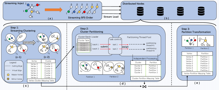
Figure 1: CLUGP Architecture

For vertex clustering, as shown in Figure 1 (c-1), vertices $v_{0}$ to $v_{6}$ are uniquely assigned to clusters $c_{0}$ to $c_{3}$, thus there exist cutting edges, but not vertex replicas. For example, $e(3,5)$ is a cutting edge generated by the vertex clustering algorithm, while $v_{3}$ and $v_{5}$ belong to clusters $c_{3}$ and $c_{1}$, respectively.

For edge partitioning, as shown in Figure 1 (c-2), two replicas of vertex $v_{0}$ and one replica of $v_{3}$ are generated, as highlighted by dashed circle. The existence of vertex replicas eliminates edge-cutting for “real” edges. The dashed lines represent virtual edges, connecting master and mirror vertices. For example, $v_{0}$ is the master vertex, and $v_{0}^{\prime}$ and $v_{0}^{\prime\prime}$ are mirror vertices and replicas of $v_{0}$. Hence, $e(v_{0},v_{0}^{\prime})$ is a virtual edge.

We therefore propose a new vertex clustering framework, tailored for minimizing vertex replicas. It produces a coarse-grained vertex-cut partitioning result, in the form of vertex-cluster pairs. Details are shown in Section IV.

III-B Second Pass: Cluster Partitioning

The second step is to assign the generated clusters to the given set of partitions, which can be formalized as follows.

Problem 3 (Cluster Partitioning).

Suppose $m$ clusters $G_{C}=\{c_{i}\}_{1\leq i\leq m}$ and $k$ partitions $P=\{p_{i}\}_{1\leq i\leq k}$. The problem is to assign each cluster $c_{i}\in G_{C}$ to a partition $p_{i}\in P$, while minimizing edge-cutting and imbalance. The output is a table mapping a cluster to a partition, $\{\langle c_{i},p_{j}\rangle\}$.

The optimization target of cluster partitioning problem has two parts, load balancing and edge-cutting minimization. For the load balancing part, without losing generality, we use $\lambda\frac{1}{k}\sum_{p_{i}\in P}|p_{i}|^{2}$ to denote imbalance cost of $k$ partitions [moons2013game, vocking2007selfish]. Parameter $\lambda$ is for normalization. It is obvious that the lowest imbalance is achieved, when partitions are of the same size. For the edge-cutting part, we can use the number of inter-partition (virtual) edges as the cost. By integrating the two costs, we can get the overall cluster partitioning cost function.

Definition 2 (Cluster Partitioning Cost).

The overall cluster partitioning cost is defined as:

$$\small Cost=\underbrace{\lambda\frac{1}{k}\sum_{p_{i}\in P}|p_{i}|^{2}}_{load~{}balancing}+\underbrace{\sum_{p_{i}\in P}|e(p_{i},V\backslash p_{i})|}_{edge-cutting}$$ (2)

where $\sum_{p_{i}\in P}|e(p_{i},V\backslash p_{i})|$ is the number of cutting edges.

It can be shown that finding the global optimal solution targeted on Equation 2 is NP-hard, by reducing it from the set cover problem. To get a sub-optimal solution, we treat each cluster as a player. Then, the cluster partitioning problem can be modelled as a strategic game. For a cluster, the selection of a partition can thus be regarded as a rational game strategy, where each cluster affects others’ costs and meanwhile minimizes its own cost by strategically manipulating its partition choice. Thus, the optimization problem is transformed into finding the Nash equilibrium of the game, so that each player/cluster minimizes its own cost.

However, the retrieval of the Nash equilibrium is compute-bound, a.k.a., the overhead of computation dominates that of I/O. So, we design a parallel strategy to accelerate the cluster partitioning process. As shown in Figure 1(d), clusters generated are grouped into batches, where each batch is executed by an independent thread to find the Nash equilibrium.

More technical details and analysis of cluster partitioning problem are covered by Section V.

III-C Third Pass: Partitioning Transformation

By joining the outputs of the first two steps, we can map a vertex to a partition. For mapping an edge to a partition, we utilize partitioning transformation as the third step of CLUGP. It accesses edge streams for further refining the cluster-based partitioning result of the second step.

Problem 4 (Partitioning Transformation).

Given the mapping table from vertices to partitions, $\{\langle v_{i},p_{j}\rangle\}=\{\langle v_{i},c_{j}\rangle\}\bowtie\{\langle c_{i},p_{j}\rangle\}$, the problem is to transform vertex mapping table $\{\langle v_{i},p_{j}\rangle\}$, to edge mapping table $\{\langle e_{i},p_{j}\rangle\}$, which serves as the partitioning result.

For each edge $e(u,v)\in G_{S}$, partitions $P(u)$ and $P(v)$ are accessed to determine which partition $e$ is assigned to. The two partitions are retrieved based on the joining results of the first two steps. Notice that we do not explicitly maintain the joining results for reducing memory cost. Instead, one can quickly map a vertex to a partition by querying the two mapping tables sequentially. The determination of $e$ assignment has been addressed in previous two steps, following the optimization target of edge-cutting and imbalance. The de facto assignment of edges is implemented in the third step, by traversing the streaming graph. The details are covered in Algorithm 1.

Algorithm 1 Partition Transformation

Input Cluster Partition Strategy $a^{*}$, Cluster Set $clu[]$, Vertex
      Degree $deg[]$, Load Balance Factor $\tau$
      Output Partition Result

1:Let $a_{i}$ be the partition choice of cluster $c_{i}$;

2:Initialize the array of load, $L_{max}=\tau\frac{|E|}{k}$;

3:for $e(u,v)\in G_{S}$ do

4:    $c_{u},c_{v}\leftarrow clu[u]$, $clu[v]$;

5:    $p_{u},p_{v}\leftarrow a_{u},a_{v}$;

6:    if $|p_{u}|\geq L_{max}$ or $|p_{v}|\geq L_{max}$ then

7:        if $|p_{u}|<L_{max}$ then

8:           assign $e$ to $p_{u}$;

9:           continue;         

10:        if $|p_{v}|<L_{max}$ then

11:           assign $e$ to $p_{v}$;

12:           continue;         

13:        for $p_{i}\in P$ do

14:           assign $e$ to $p_{i}$ if $|p_{i}|<L_{max}$; $\rhd$ Load Balance         

15:    else if $p_{u}$ equal $p_{v}$ then

16:        assign $e$ to $p_{u}$ 

17:    else

18:        if either $u$ or $v$ has mirror vertices then

19:           assign $e$ to $p_{v}$ or $p_{u}$;

20:        else

21:           assign $e$ to $p_{u}$ if $deg[v]>deg[u]$;

22:           assign $e$ to $p_{v}$ if $deg[u]>deg[v]$; $\rhd$ Reduce Replicas             

For each edge $e(u,v)$, if neither of $P(u)$ and $P(v)$ can accommodate $e$, then $e$ will be assigned to an underflow partition, for workload balancing (lines 6-14). When $u$ and $v$ are in the same partition, $e$ will be assigned to the partition (lines 15-16). If $u(v)$ has mirror vertices, which means the vertex $u(v)$ has been replicate during step 1 (Section IV), $e$ will be assigned to the partitions where $u(v)^{\prime}s$ mirror vertex belongs to (lines 18-19). Otherwise, the vertex with a higher degree will be cut (lines 21-22) to reduce vertex replicas, similar to [petroni2015hdrf, mayer2018adwise, patwary2019window].

During the transformation, there is a user-specified parameter, i.e., imbalance factor $\tau$, on controlling the partition size. Compared to $\tau$, $V_{max}$ of the first step is merely the upper limit of cluster capacities. The purpose of $\tau$ is to further improve partition balancing from coarse-grained cluster-level to fine-grained partition-level. This way, edges that incur partitioning overflowing are moved to underflow partitions, strictly conforming to the system parameter $\tau$.

For the third step, CLUGP traverses the edge stream to perform partition transformation that merely takes $O(1)$ space cost, since we only need a $k$ elements array to store the partition size. To perform transformation, the query over vertex-to-partition mapping tables only takes $O(1)$ time for each edge. The total time complexity is $O(|E|)$.

This way, our architecture can be well parallelized. Of the system, each distributed node accesses partial streaming edges and performs the three steps, clustering, game processing, and transformation, locally. Further, game processing of a distributed node can be parallelized by multi-threading. After the three steps, the final graph partitioning result is obtained by combining the partial partitioning results of distributed nodes.

IV Streaming Clustering

In this section, we investigate a new streaming clustering algorithm. In particular, we propose the allocation-splitting-migration framework in Section IV-A, and conduct theoretical analysis in Section IV-B.

IV-A Allocation-splitting-migration Framework

The first and only streaming version of graph clustering algorithm, Holl, is proposed by Hollocou et al. [hollocou2017streaming].

Holl presented an allocation-migration framework for streaming clustering. However, Holl cannot be directly applied for graph partitioning, because the allocation-migration framework of Holl incurs high replication factors. CLUGP improves Holl by adding a splitting operation, and thus construct a new allocation-splitting-migration. We will prove that the splitting operation can decrease the replication factor.

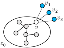
(a) before splitting

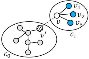
(b) CLUGP with splitting

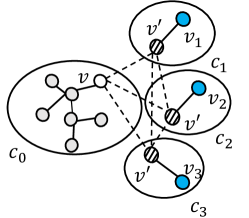
(c) Holl without splitting

Figure 2: An Example of Cluster Splitting for Streaming Clustering (Vertex IDs follow BFS order, e.g., $G_{S}=\{e(v,v_{1}),e(v,v_{2}),e(v,v_{3}),\cdots\}$

Consider the example in Figure 2. Suppose cluster $c_{0}$ reaches the maximum cluster volume $V_{max}$, in Figure 2(a). In Holl, to handle incoming edges $e(v,v_{1})$, $e(v,v_{2})$, and $e(v,v_{3})$, cluster $c_{0}$ remains as it is, while new clusters, $c_{1}$, $c_{2}$, and $c_{3}$, are generated to accommodate successive streaming edges, as shown in Figure 2(c). According to the allocation-migration mechanism of Holl, cluster $c_{0}$ never splits, so that the master vertex of $v$ is always subordinated to $c_{0}$, and the mirror vertex $v^{\prime}$ exists in $c_{1}$ to $c_{3}$. After clustering, the number of master vertices is $10$, and the number of mirror vertices is $3$. Based on Equation 1, the replication factor of Holl is $\frac{10+3}{10}=\frac{13}{10}$.

CLUGP adds a splitting operation, as highlighted in Algorithm 2. The splitting operation can effectively chop high-degree vertices to reduce replicas in the streaming clustering process, since high-degree vertices tend to form new clusters with subsequent neighboring vertices. In Figure 2 (b), with the splitting operation, $c_{0}$ is split into two clusters, $c_{0}$ and $c_{1}$, and the master vertex of $v$ is assigned to new cluster $c_{1}$ meanwhile generating a mirror vertex $v^{\prime}$ in $c_{0}$. In this case, the replication factor of CLUGP is $\frac{11}{10}$, which is smaller than that of Holl.

Algorithm 2 Streaming Graph Clustering of CLUGP

Input Edge Stream $G_{S}$, Maximum Cluster Volume $V_{max}=\frac{|E|}{k}$
      Output Cluster Set $G_{C}$, Cluster ID $clu[]$, Vertex Degree $deg[]$

1:Initialize the array of degree, cluster, and volume;

2:$vol(c_{i})$ returns the volume of cluster $c_{i}$ 

3:for $e(u,v)\in G_{S}$ do

4:    if $clu[u]$ is NULL or $clu[v]$ is NULL then

5:        Assign a new cluster ID for $u$ or $v$;     

6:    $c_{u}\leftarrow clu[u]$, $c_{v}\leftarrow clu[v]$;

7:    $deg[u]\leftarrow deg[u]+1$, $deg[v]\leftarrow deg[v]+1$;

8:    $vol(c_{u})\leftarrow vol(c_{u})+1$, $vol(c_{v})\leftarrow vol(c_{v})+1$;

9:    if $vol(c_{u})\geq V_{max}$ then

10:        Assign a new cluster ID for $u$;

11:        $c_{u}^{\prime}\leftarrow clu[u]$, mark $u$ as divided vertex;

12:        $vol(c_{u})\leftarrow vol(c_{u})-deg[u]$;

13:        $vol(c_{u}^{\prime})\leftarrow vol(c_{u}^{\prime})+deg[u]$;     

14:    if $vol(c_{v})\geq V_{max}$ then

15:        Assign a new cluster ID for $v$;

16:        $c_{v}^{\prime}\leftarrow clu[v]$, mark $v$ as divided vertex;

17:        $vol(c_{v})\leftarrow vol(c_{v})-deg[v]$;

18:        $vol(c_{v}^{\prime})\leftarrow vol(c_{v}^{\prime})+deg[u]$;     

19:    $c_{u}\leftarrow clu[u]$, $c_{v}\leftarrow clu[v]$;

20:    if $vol(c_{u})<V_{max}$ and $vol(c_{v})<V_{max}$ then

21:        if $vol(c_{u})\leq$ $vol(c_{v})$ then

22:           Migrate $u$ from $c_{u}$ to $c_{v}$;

23:           Update $vol(c_{u})$ and $vol(c_{v})$;

24:        else

25:           Migrate $v$ from $c_{v}$ to $c_{u}$;

26:           Update $vol(c_{u})$ and $vol(c_{v})$;             return $G_{C}$

The details about the improved streaming clustering algorithm of CLUGP are covered in Algorithm 2. The clustering process builds clusters in a bottom-up manner, where each cluster initially has one vertex. For an incoming edge $e(u,v)$ of streaming $G_{S}$, the two incident vertices of $e$ are assigned to two clusters $c_{u}$ and $c_{v}$ (lines 3-5). The volume of a cluster is defined as the sum of the degrees of master vertices in the cluster. A cluster overflows, if the volume of a cluster exceeds its maximum capacity ($V_{max}$). Holl handles cluster overflowing, by assigning incoming edges to a new cluster. CLUGP handles cluster overflowing, by splitting the original cluster into two smaller clusters for generating fewer replicas (lines 9-19). At last, the algorithm migrates an incident vertex of edge $e$ from a smaller cluster to a bigger cluster (lines 20-26). The process repeats until all incoming edges of $G_{S}$ are processed, so that the cluster set $G_{C}$ is generated as the output.

In the streaming clustering step, we use the vertex-cluster mapping table to store the cluster that a vertex belongs to. To get the degree of vertices, we also need an array to record the degree. So, the space cost of this step is $O(|V|)$. The time cost of modifying and querying the mapping table or degree array is $O(1)$. The process traverses all incoming edges, so the time cost of Algorithm 2 is $O(|E|)$.

During the splitting operation, we mark the vertex that causes cluster splitting as divided vertex (lines $11$, $16$). Then, we can quickly find which vertex has been replicated and which cluster its mirror vertices belongs to. In Figure 2 (b), during the clustering step, vertex $v$ is marked as a divided vertex. So, when processing edge $e(v,v_{1})$, we can quickly find that $e(v,v_{1})$ should be assigned to $c_{1}$ and generate a mirror vertex $v^{\prime}$ in $c_{0}$, thus there exists a cutting edge between $c_{0}$ and $c_{1}$ (denoted as dashed lines). By the way, when both vertices of an edge are marked as divided vertices, we split the vertex with a higher degree vertex and assign the edge to the cluster where lower degree vertex belongs to, which is shown to be effective in reducing replication factor for power-law graphs [petroni2015hdrf, patwary2019window, mayer2018adwise].

We can get two facts from Algorithm 2: a) allocation and splitting operations increase at most one vertex replica at an iteration; b) migration operation reduces at most one vertex replica at an iteration. But, a seemingly plausible observation, that the splitting operation triggers more vertex replicas, is not correct, because the splitting operation of CLUGP can reduce total number of replicas. This is guaranteed by Algorithm 2. First, if the splitting operation is not triggered, CLUGP is degenerated into Holl, so that the two have the same replication factor. Second, if the splitting operation is triggered, CLUGP can derive a smaller replication factor than Holl. In summary, CLUGP derives a smaller replication factor than Holl.

IV-B Analysis

We prove that CLUGP can effectively reduce the replicate factor, based on the properties for power-law graphs. According to [cohen2001breakdown], for a power-law graph, if we remove $\frac{1}{\theta}$ of vertices with the highest degrees, then the maximum degree $\tilde{M}$ of the remnant subgraph can be approximated by $\tilde{M}=\gamma{\theta}^{1/(1-\alpha)}$, where $\gamma$ is the global minimum degree, and $\alpha$ is the exponent of the power-law graph. Based on this property, we can get that, given a specific degree $d$, the fraction $\theta$ of vertices satisfying $\{v|degree(v)\geq d\}$, is:

$$\footnotesize\theta=\left(\frac{\gamma}{d-1}\right)^{\alpha-1}$$ (3)

Equation 3 can be used for describing the worst case of CLUGP, a.k.a., the highest replication factor of the splitting operation. The details are covered in Theorem 1.

Theorem 1.

The upper bound of replication factor of CLUGP is always no larger than that of Holl.

Proof.

To prove the theorem, we only need to show that, the upper bound of replicate factor of CLUGP is no larger than the replication factor of Holl, $RF_{clugp}\leq RF_{holl}$.

Given the number of replicas $r$ of vertex $v$, we have $degree(v)\geq d_{min}^{clugp}(r)$, where $d_{min}^{clugp}(r)$ denotes the minimum degree of the vertex $v$, if $v$ has been replicated $r$ times. Based on Equation 3, we can get the maximum number of vertices with $r$ replicas equals to $|V|\left(\frac{\gamma}{d_{min}^{clugp}(r)-1}\right)^{\alpha-1}$, by multiplying $|V|$ with $\theta$.

Considering the worst case, let the number of clusters be $m$, for any vertex $v$ with degree $degree(v)$, there can be most $max(degree(v)-1,m-1)$ replicas for $v$. If the $degree(v)$ less than $m$, the worst case can be happened when all $degree(v)$ edges of the vertex are assigned to different clusters. Otherwise, each cluster $\{c_{i}\}_{1\leq i\leq m}$ has an edge (mirror vertex) of $v$. So, a sequence of maximum replicas can be generated by vertices is $\{m-1,m-2,\cdots,\gamma-1\}$, each replica corresponds to a fraction of vertices $\theta_{r}^{clugp}=\left(\frac{\gamma}{d_{min}^{clugp}(r)-1}\right)^{\alpha-1}$, where $\gamma-1\leq r\leq m-1$. Thus, we can get the upper bound of replicate factor of CLUGP as follows.

$$\footnotesize\begin{split}RF_{clugp}\leq&(m-1)\cdot\theta_{m-1}^{clugp}+(m-2)\cdot(\theta_{m-2}^{clugp}-\theta_{m-1}^{clugp})\\ &+\dots+(m-\gamma)(\theta_{\gamma-1}^{clugp}-\theta_{\gamma}^{clugp})\\ =&\theta_{m-1}^{clugp}+\dots+\theta_{\gamma}^{clugp}+(m-\gamma)\cdot\theta_{\gamma-1}^{clugp}\\ \end{split}$$ (4)

Similarly, for Hollocou’s algorithm, we can have that:

$$\footnotesize\begin{split}RF_{holl}\leq&\theta_{m-1}^{holl}+\dots+\theta_{\gamma}^{holl}+(m-\gamma)\cdot\theta_{\gamma-1}^{holl}\\ \end{split}$$ (5)

Based on Theorem 2, we know that $d_{min}^{clugp}(r\geq 2)>d_{min}^{holl}(r\geq 2)$. Substituting it into Equation 3, we get $\theta_{r}^{clugp}\leq\theta_{r}^{holl}$, then combining it into Equations 4, 5, we can get $RF_{clugp}\leq RF_{holl}$. So, the theorem is proved. ∎

Theorem 2.

Suppose two vertices $v_{c},v_{h}\in V$, where $v_{c}$ and $v_{h}$ are processed by CLUGP and Holl, respectively. If $v_{c}$ and $v_{h}$ are both with $r$ replicas, the minimum degree of $v_{c}$ must be no less than that of $v_{h}$. Formally, $d_{min}^{clugp}(r)\geq d_{min}^{holl}(r)$.

Proof.

Let $R(v)$ denotes the number of replicas of vertex $v$. For CLUGP, it can be obviously seen from Figure 2(b) that, if $R(v)=0$, it means the vertex $v$ does not need any replicate, so we have $d_{min}^{clugp}(r)=1$, if $R(v)=1$, it means the vertex $v$ has at least one splitting operation, so we have $d_{min}^{clugp}(r)=2$. Similarly, when $R(v)=2$, it means we must fill up the cluster $c_{1}$ and split the vertex $v$ out of $c_{1}$. To better prove the theorem, we let the degree of $v$’s neighbors equal to the global maximum degree $d_{max}$, which is the worst case of CLUGP, since the splitting operation can be triggered intensively. So on when $R(v)=r\geq 2$ we have the following equation sets:

$$\left\{\begin{array}[]{lr}1+|Ne_{1}|+|Ne_{1}|\cdot d_{max}&=V_{max}\\ 1+|Ne_{1}|+|Ne_{2}|+|Ne_{2}|\cdot d_{max}&=V_{max}\\ 1+|Ne_{1}|+|Ne_{2}|+|Ne_{3}|+|Ne_{3}|\cdot d_{max}&=V_{max}\\ &\vdots\\ 1+|Ne_{1}|+\dots+|Ne_{r-2}|+|Ne_{r-1}|\cdot d_{max}&=V_{max}\\ |Ne_{r}|&=1\\ \end{array}\right.$$ (6)

, where $|Ne_{i}|$ denotes the number of neighbor vertices that vertex $v$ needed to fill up the cluster $c_{i}$. And next, we can get the solution as follows:

$$\small\left\{\begin{array}[]{lr}|Ne_{i}|=\frac{V_{max}-1}{d_{max}}\cdot(\frac{d_{max}}{1+d_{max}})^{i}&,1\leq i\leq r-1\\ |Ne_{i}|=1&,i=r\\ \end{array}\right.$$ (7)

After summing the number of edges needed for $v$, we have:

$$\small\begin{split}d_{min}^{clugp}(r\geq 2)&=1+|Ne_{1}|+\dots+|Ne_{r-1}|+|Ne_{r}|\\ &=(V_{max}-1)\left[1-(1-\frac{1}{1+d_{max}})^{r-1}\right]+2\\ \end{split}$$ (8)

That is, if a vertex $v$ has been replicated $r\geq 2$ times, the degree of $v$ must satisfy $degree(v)\geq d_{min}^{clugp}(r)$. For Holl, since it does not have splitting operation to migrate vertex $v$ out of $c_{0}$, each neighbour of vertex $v$ will be allocated a independent cluster, thus, we can easily get that $d_{min}^{holl}(r\geq 2)=r-1$. Additionally, $d_{min}^{holl}(r)=d_{min}^{clugp}(r)$ when $r\leq 1$, so we only consider the situation that $r\geq 2$. Since for power-law graph $d_{max}\gg 1$, $r-1>0$, thus $\frac{1}{1+d_{max}}\to 0$ and we can get $(1-\frac{1}{1+d_{max}})^{r-1}\sim 1-\frac{r-1}{1+d_{max}}$. Therefore, we can get that:

$$\small\begin{split}d_{min}^{clugp}(r\geq 2)&=(V_{max}-1)\left[1-(1-\frac{1}{1+d_{max}})^{r-1}\right]+2\\ &=(V_{max}-1)\cdot(\frac{r-1}{1+d_{max}})+2\\ &>(1+d_{max})\cdot(\frac{r-1}{1+d_{max}})+2\\ &=r+1>r-1=d_{min}^{holl}(r\geq 2)\\ \end{split}$$ (9)

where $V_{max}=\frac{|E|}{k}>d_{max}$. Hence, the theorem is proved. ∎

V Game Theory-based Cluster Partitioning

In this section, we study a suboptimal solution for the problem of cluster partitioning. We formalize the problem of cluster partitioning and prove the existence of Nash equilibrium in Section V-A. We theoretically prove the quality guarantee for the game in Section LABEL:subsec:analysis.

V-A Modeling of Cluster Partitioning Problem

In strategic games, a player aims to choose the strategy that minimizes his/her own individual cost. The game continues until a steady state is achieved, in which no player can benefit by unilaterally changing its strategy.

In our work, clusters $\{c_{i}\}_{i\leq m}$ can be considered as independent and competing players in a strategy game. For each cluster $c_{i}$, there can be $k$ choices for choosing a partition. Let strategy $a_{i}$ be the partition choice of cluster $c_{i}$. Then, the strategy profile $\Lambda=\{a_{i}\}_{i\leq m}$ consists of the strategies for all clusters. For a fixed strategy profile $\Lambda$, each strategy $a_{i}\in\Lambda$ refers to the partition that $c_{i}$ belongs to. We use $|a_{i}|$ to represent the number of edges of the partition that $c_{i}$ belongs to. For example, if $a_{i}$ refers to $p_{j}$, $|a_{i}|$ equals to the size of $p_{j}$, i.e., $|e(p_{j},p_{j})|$.

Given a strategy profile $\Lambda$, the global deployment cost is denoted as $\varphi(\Lambda)$, and the deployment cost of each cluster $c_{i}$ is denoted as $\varphi(a_{i})$. Intuitively, a lower deployment cost corresponds to a higher partition quality. Based on the cluster partitioning optimization target (Equation 2), the global deployment target $\varphi(\Lambda)$ can be defined as:

$$\varphi(\Lambda)=\underbrace{\lambda\frac{1}{k}\sum_{i=1}^{k}|p_{i}|^{2}}_{load~{}balancing}+\underbrace{\sum_{i=1}^{k}|e(p_{i},V\backslash p_{i})|}_{edge-cutting}$$ (10)

The game-based solution ensures that the global partitioning optimization target $\varphi(\Lambda)$ (Equation 10) can be achieved, if each cluster $c_{i}$’s locally minimized partitioning cost $\varphi(a_{i})$ is achieved. We first explain the local optimization target for each cluster/player. Then, we prove that the local optimization targets of clusters can be integrated as the global target.

The local cost of a cluster has two parts, load balancing and edge-cutting (Equation V-A), which is consistent with the form of the global cost function $\varphi(\Lambda)$ (Equation 10).

We use variable $|c_{i}|$ to denote the number of edges of cluster $c_{i}$, formally, $|c_{i}|=|e(c_{i},c_{i})|$. To ensure the load balance, we should assign the large-scale clusters to the partitions with small size. So, for each cluster $c_{i}$ and its partition $a_{i}$, the cost of imbalance can be defined as $\varphi^{load}(a_{i})=\frac{1}{k}|c_{i}||a_{i}|$. To reduce the number of cut edges, the cluster $c_{i}$ should be placed in the partition that has the least number of cut edges from other partitions. Therefore, the cost of edge-cut can be defined as $\varphi^{cut}(a_{i})=\frac{1}{2}(|e(c_{i},V\backslash a_{i})|+|e(V\backslash a_{i},c_{i})|)$. In conclusion, we can get a cluster $c_{i}$’s cost under the partition $a_{i}$.

$$\footnotesize\varphi(a_{i})= \lambda\varphi^{load}(a_{i})+\varphi^{cut}(a_{i})$$

$$= \underbrace{\frac{\lambda}{k}|c_{i}|\cdot|a_{i}|}_{load~{}balancing}+\underbrace{\frac{1}{2}(|e(c_{i},V\backslash a_{i})|+|e(V\backslash a_{i},c_{i})|)}_{edge-cutting}$$ (11)

We next show how the local cost function (Equation V-A) can be derived from the global cost function (Equation 10).

$$\footnotesize\begin{split}\varphi(\Lambda)=&\lambda\frac{1}{k}\sum_{i=1}^{k}\sum_{c_{j}\in p_{i}}|c_{j}||p_{i}|+\frac{1}{2}\sum_{i=1}^{k}(|e(p_{i},V\backslash p_{i})|+|e(V\backslash p_{i},p_{i})|)\\ =&\lambda\frac{1}{k}\sum_{i=1}^{m}|c_{i}||a_{i}|+\frac{1}{2}\sum_{i=1}^{k}\sum_{c_{j}\in p_{i}}(|e(c_{j},V\backslash a_{j})|+|e(V\backslash a_{j},c_{j})|)\\ =&\lambda\frac{1}{k}\sum_{i=1}^{m}|c_{i}||a_{i}|+\frac{1}{2}\sum_{i=1}^{m}(|e(c_{i},V\backslash a_{i})|+|e(V\backslash a_{i},c_{i})|)\\ =&\lambda\sum_{i=1}^{m}\varphi^{load}(a_{i})+\sum_{i=1}^{m}\varphi^{cut}(a_{i})=\sum_{i=1}^{m}\varphi(a_{i})\end{split}$$ (12)

Consequently, minimizing the global deployment cost is equivalent to minimizing the set of individual deployment costs. Then, we can define the Nash equilibrium of the cluster partitioning game as follows.

Definition 3 (Nash equilibrium).

A strategy decision profile $\Lambda^{*}=\{a_{1}^{*},a_{2}^{*},\cdots,a_{m}^{*}\}$ of all clusters is a Nash equilibrium [nash1950equilibrium], if all clusters achieve their locally optimization targets. This way, no cluster has an incentive for unilaterally deviating the strategy for a lower cost.

Algorithm 3 Nash equilibrium

Input Cluster Set $G_{C}$, Partition Set $P$, Cluster Neighbors $N[]$
      Output Nash equilibrium

1:Initial individual cost for each cluster.

2:Assign each cluster $c_{i}\in G_{C}$ to a random partition.