A General Framework for Treatment Effect Estimation in Semi-supervised and High Dimensional Settings

Abstract

In this article, we aim to provide a general and complete understanding of semi-supervised (SS) causal inference for treatment effects, using two such estimands as prototype cases. Specifically, we consider estimation of: (a) the average treatment effect and (b) the quantile treatment effect, in an SS setting, which is characterized by two available data sets: (i) a labeled data set of size $n$, providing observations for a response and a set of potentially high dimensional covariates, as well as a binary treatment indicator; and (ii) an unlabeled data set of size $N$, much larger than $n$, but without the response observed. Using these two data sets, we develop a family of SS estimators which are guaranteed to be: (1) more robust and (2) more efficient, than their supervised counterparts based on the the labeled data set only. Moreover, beyond the “standard” double robustness results (in terms of consistency) that can be achieved by supervised methods as well, we further establish root-$n$ consistency and asymptotic normality of our SS estimators whenever the propensity score in the model is correctly specified, without requiring specific forms of the nuisance functions involved. Such an improvement in robustness arises from the use of the massive unlabeled data, so it is generally not attainable in a purely supervised setting. In addition, our estimators are shown to be semi-parametrically efficient also as long as all the nuisance functions are correctly specified. Moreover, as an illustration of the nuisance function estimation, we consider inverse-probability-weighting type kernel smoothing estimators involving possibly unknown covariate transformation mechanisms, and establish in high dimensional scenarios novel results on their uniform convergence rates. These results should be of independent interest. Numerical results on both simulated and real data validate the advantage of our methods over their supervised counterparts with respect to both robustness and efficiency.

, and

1 Introduction

Semi-supervised (SS) learning has received increasing attention as one of the most promising areas in statistics and machine learning in recent years. We refer interested readers to Zhu (2005) and Chapelle, Schölkopf and Zien (2010) for a detailed overview on this topic, including its definition, goals, applications and the fast growing literature. Unlike traditional supervised or unsupervised learning settings, an SS setting, as the name suggests, represents a confluence of these two kinds of settings, in the sense that it involves two data sets: (i) a labeled data set $\mathcal{L}$ containing observations for an outcome $\mathbb{Y}$ and a set of covariates ${\mathbf{X}}$ (that are possibly high dimensional), and (ii) a much larger unlabeled data set $\mathcal{U}$ where only ${\mathbf{X}}$ is observed. Such situations arise naturally when ${\mathbf{X}}$ is easily available for a large number of individuals while the corresponding observations for $\mathbb{Y}$ are much harder to collect owing to cost or time constraints. The SS setting is common to a broad class of practical problems in the modern era of “big data”, including machine learning applications like text mining, web page classification, speech recognition, natural language processing etc.

Among biomedical applications, SS settings have turned out to be increasingly relevant in modern integrative genomics, especially in expression quantitative trait loci (eQTL) studies (Michaelson, Loguercio and Beyer, 2009) combining genetic association studies with gene expression profiling. These have become instrumental in understanding various important questions in genomics, including gene regulatory networks (Gilad, Rifkin and Pritchard, 2008; Hormozdiari et al., 2016). However, one issue with such studies is that they are often under-powered due to the limited size of the gene expression data which are expensive (Flutre et al., 2013). On the other hand, records on the genetic variants are cheaper and often available for a massive cohort, thus naturally leading to SS settings while necessitating robust and efficient strategies that can leverage this extra information to produce more powerful association mapping tools as well as methods for detecting the causal effects of the genetic variants. Moreover, SS settings also have great relevance in the analysis of electronic health records data, which are popular resources for discovery research but also suffer from a major bottleneck in obtaining validated outcomes due to logistical constraints; see, e.g., Chakrabortty and Cai (2018) and Cheng, Ananthakrishnan and Cai (2020) for more details.

1.1 Problem setup

In this paper, we consider causal inference problems in SS settings. To characterize the basic setup, suppose our sample consists of two independent data sets: the labeled (or supervised) data $\mathcal{L}:=\{(\mathbb{Y}_{i},T_{i},{\mathbf{X}}_{i}^{\rm T})^{\rm T}:i=1,\ldots,n\}$, and the unlabeled (or unsupervised) data $\mathcal{U}:=\{(T_{i},{\mathbf{X}}^{\rm T}_{i})^{\rm T}:i=n+1,\ldots,n+N\}$ (with $N\gg n$ possibly), containing $n$ and $N$ independent copies of ${\mathbf{Z}}:=(\mathbb{Y},T,{\mathbf{X}}^{\rm T})^{\rm T}$ and $(T,{\mathbf{X}}^{\rm T})^{\rm T}$, respectively, where $T\in\{0,1\}$ serves as a treatment indicator, i.e., $T=1$ or $0$ represents whether an individual is treated or not. (Note: Though not the main focus of this paper, we also consider the setting where the treatment $T$ is unobserved in $\mathcal{U}$, in Section 2.4.) The covariates (often also called confounders) ${\mathbf{X}}\in{\cal X}\subset\mathbb{R}^{p}$ are (possibly) high dimensional, with dimension $p\equiv p_{n}$ allowed to diverge and possibly exceed $n$ (including $p\gg n$), while the observed outcome is given by:

$$\mathbb{Y}~{}:=~{}TY(1)+(1-T)Y(0),$$

where $Y(t)$ is the potential outcome of an individual with $T=t$ $(t=0,1)$ (Rubin, 1974; Imbens and Rubin, 2015). Thus, $(\mathbb{Y}\mid T=t)~{}\equiv~{}Y(t)$ (also called the consistency assumption).

A major challenge (and a key feature) in the above framework arises from the (possibly) disproportionate sizes of $\mathcal{L}$ and $\mathcal{U}$, namely $|\mathcal{U}|\gg|\mathcal{L}|$, an issue widely encountered in modern (often digitally recorded) observational datasets of massive sizes, such as electronic health records (Cheng, Ananthakrishnan and Cai, 2020). We therefore assume (rather, allow for):

$$\nu~{}:=~{}\hbox{$\lim_{n,{\color[rgb]{0,0,0}N}\to\infty}$}n/(n+N)~{}=~{}0,$$ (1)

as in Chakrabortty and Cai (2018) and Gronsbell and Cai (2018). An example of (1) is the ideal SS setting where $n<\infty$ and $N=\infty$ (i.e., the distribution of $(T,{\mathbf{X}}^{\rm T})^{\rm T}$ is known). Essentially, the condition (1) distinguishes our framework from that of traditional missing data theory, which typically requires the proportion of complete cases in the sample to be bounded away from zero – often known as the “positivity condition” (Imbens, 2004; Tsiatis, 2007). The natural violation of this condition in SS settings is what makes them unique and more challenging than traditional missing data problems. On the other hand, we do assume throughout this paper that $\mathcal{L}$ and $\mathcal{U}$ have the same underlying distribution (i.e., $\mathbb{Y}$ in $\mathcal{U}$ are missing completely at random) which is the typical (and often implicit) setup in the traditional SS literature (Zhu, 2005; Chapelle, Schölkopf and Zien, 2010). We formalize this below.

Assumption 1.1.

The observations in $\mathcal{L}$ and $\mathcal{U}$ have the same underlying distribution, so that $\{(\mathbb{Y}_{i},T_{i},{\mathbf{X}}_{i}^{\rm T})^{\rm T}:i=1,\ldots,n\}$ and $\{(T_{i},{\mathbf{X}}_{i}^{\rm T})^{\rm T}:i=n+1,\ldots,n+N\}$ respectively are $n$ and $N$ independent realizations from the distributions of $(\mathbb{Y},T,{\mathbf{X}}^{\rm T})^{\rm T}$ and $(T,{\mathbf{X}}^{\rm T})^{\rm T}$.

Causal parameters of interest

Based on the available data $\mathcal{L}\cup\mathcal{U}$, we aim to estimate: (i) the average treatment effect (ATE):

$$\mu_{0}(1)-\mu_{0}(0)~{}:=~{}\mathbb{E}\{Y(1)\}-\mathbb{E}\{Y(0)\},{\color[rgb]{0,0,0}~{}~{}\mbox{and}}$$ (2)

(ii) the quantile treatment effect (QTE):

$$\theta_{0}(1,\tau)-\theta_{0}(0,\tau)~{}\equiv~{}\theta_{0}(1)-\theta_{0}(0),$$ (3)

where $\theta_{0}(t,\tau)\equiv\theta_{0}(t)$ represents the $\tau$-quantile of $Y(t)$ for some fixed and known $\tau\in(0,1)$, defined as the solution to the equation:

$$\mathbb{E}[\psi\{Y(t),\theta_{0}(t,\tau)\}]~{}:=~{}\mathbb{E}[I\{Y(t)<\theta_{0}(t,\tau)\}-\tau]~{}=~{}0\quad(t=0,1){\color[rgb]{0,0,0},}$$ (4)

with $I(\cdot)$ being the indicator function. It is worth noting that by setting $T\equiv 1$ and $\mu_{0}(0)=\theta_{0}(0)\equiv 0$, the above problems also cover SS estimation of the response mean and quantile as special cases. The ATE and the QTE are both well-studied choices of causal estimands in supervised settings; see Section 1.2 for an overview of these literature(s). While the ATE is perhaps the more common choice, the QTE is often more useful and informative, especially in settings where the causal effect of the treatment is heterogeneous and/or the outcome distribution(s) is highly skewed so that the average causal effect may be of limited value.

Our goal here, in general, is to investigate how, when, and to what extent, one can exploit the full data $\mathcal{L}\cup\mathcal{U}$ to develop SS estimators of these parameters that can “improve” standard supervised approaches using $\mathcal{L}$ only, where the term “improve” could be in terms of efficiency or robustness or both. The rest of this paper is dedicated to a thorough understanding of such questions via a complete characterization of the possible SS estimators and their properties.

We also clarify here that we choose the ATE and QTE as two representative causal estimands – presenting diverse methodological and technical challenges – to exemplify the key features of our SS approach and its benefits, without compromising much on the clarity of the main messages. Extensions to other more general functionals (such as those based on general estimating equations) are indeed possible – as we discuss later in Section 7 and Appendix A – though we skip a detailed technical analysis for the sake of brevity and minimal obfuscation.

Basic assumptions

To ensure that the parameters $\{\mu_{0}(t),\theta_{0}(t)\}_{t=0}^{1}$ are identifiable and estimable from the observed data, we make the following standard assumptions (Imbens, 2004):

$$T\mathchoice{\mathrel{\hbox to0.0pt{$\displaystyle\perp$\hss}\mkern 4.0mu{\displaystyle\perp}}}{\mathrel{\hbox to0.0pt{$\textstyle\perp$\hss}\mkern 4.0mu{\textstyle\perp}}}{\mathrel{\hbox to0.0pt{$\scriptstyle\perp$\hss}\mkern 4.0mu{\scriptstyle\perp}}}{\mathrel{\hbox to0.0pt{$\scriptscriptstyle\perp$\hss}\mkern 4.0mu{\scriptscriptstyle\perp}}}\{Y(0),Y(1)\}\mid{\mathbf{X}},\quad\mbox{and}\quad\pi({\mathbf{x}})~{}:=~{}\mathbb{E}(T\mid{\mathbf{X}}={\mathbf{x}})~{}\in(c,1-c){\color[rgb]{0,0,0},}$$ (5)

for any ${\mathbf{x}}\in{\cal X}$ and some constant $c\in(0,1)$. The quantity $\pi({\mathbf{x}})$ is also known as the propensity score for the treatment. (5) encodes some well known conditions (Imbens and Rubin, 2015). The first part of (5) is often known as the no unmeasured confounding assumption, equivalent to the missing at random assumption in the context of missing data (Tsiatis, 2007; Little and Rubin, 2019), while the second part is the positivity (or overlap) assumption on the treatment.

Clarification

Considering that the corresponding case of $Y(0)$ is analogous, we would henceforth focus on the mean and quantile estimation of $Y(1)$ without loss of generality, and

let $$\{Y,\mu_{0},\theta_{0}\} \{Y(1),\mu_{0}(1),\theta_{0}(1)\}$$  generically denote  . (6)

1.2 Related literature

The setup and contributions of our work naturally relate to three different facets of existing literature, namely: (a) “traditional” (non-causal) SS inference, (b) supervised causal inference, and finally, (c) SS causal inference. Below we briefly summarize the relevant works in each of these areas, followed by a detailed account of our contributions.

SS learning and inference

For estimation in an SS setup, the primary and most critical goal is to investigate when and how its robustness and efficiency can be improved, compared to supervised methods using the labeled data $\mathcal{L}$ only, by exploiting the unlabeled data $\mathcal{U}$. Chapter 2 of Chakrabortty (2016) provided an elaborate discussion on this question, claiming that the answer is generally determined by the nature of the relationship between the parameter of interest and the marginal distribution, ${\mathbb{P}}_{\mathbf{X}}$, of ${\mathbf{X}}$, as $\mathcal{U}$ provides information regarding ${\mathbb{P}}_{\mathbf{X}}$ only. Therefore, many existing algorithms for SS learning that target $\mathbb{E}(\mathbb{Y}\mid{\mathbf{X}})$, including, for instance, generative modeling (Nigam et al., 2000; Nigam, 2001), graph-based methods (Zhu, 2005) and manifold regularization (Belkin, Niyogi and Sindhwani, 2006), rely to some extent on assumptions relating ${\mathbb{P}}_{\mathbf{X}}$ to the conditional distribution of $\mathbb{Y}$ given ${\mathbf{X}}$. When these assumptions are violated, however, they may perform even worse than the corresponding supervised methods (Cozman and Cohen, 2001; Cozman, Cohen and Cirelo, 2003). Such undesirable degradation highlights the need for safe usage of the unlabeled data $\mathcal{U}$. To achieve this goal, Chakrabortty and Cai (2018) advocated the robust and adaptive property for SS approaches, i.e., being consistent for the target parameters while being at least as efficient as their supervised counterparts and more efficient whenever possible. Adopting such a perspective explicitly or implicitly, robust and adaptive procedures for SS estimation and inference have been developed under the semi-parametric framework recently for various problems, including mean estimation (Zhang, Brown and Cai, 2019; Zhang and Bradic, 2019), linear regression (Azriel et al., 2016; Chakrabortty and Cai, 2018), general $Z$-estimation (Kawakita and Kanamori, 2013; Chakrabortty, 2016), prediction accuracy evaluation (Gronsbell and Cai, 2018) and covariance functionals (Cai and Guo, 2020; Chan et al., 2020). However, different from our work considering causal inference and treatment effect estimation, most of this recent progress focused on relatively “standard” (non-causal) problems defined without the potential outcome framework (and its ensuing challenges, e.g., confounding, and the missingness of one of the potential outcomes induced by the treatment assignment $T$).

Average treatment effect

Both the ATE and the QTE are fundamental and popular causal estimands which have been extensively studied in the context of supervised causal inference based on a wide range of approaches; see Imbens (2004) and Tsiatis (2007) for an overview of the ATE literature. In particular, these include inverse probability weighted (IPW) approaches (Rosenbaum and Rubin, 1983, 1984; Robins, Rotnitzky and Zhao, 1994; Hahn, 1998; Hirano, Imbens and Ridder, 2003; Ertefaie, Hejazi and van der Laan, 2020) involving approximation of the propensity score $\pi({\mathbf{X}})$, as well as doubly robust (DR) methods (Robins, Rotnitzky and Zhao, 1994; Robins and Rotnitzky, 1995; Rotnitzky, Robins and Scharfstein, 1998; Scharfstein, Rotnitzky and Robins, 1999; Kang et al., 2007; Vermeulen and Vansteelandt, 2015) which require estimating both $\mathbb{E}(Y\mid{\mathbf{X}})$ and $\pi({\mathbf{X}})$. As the name implies, the DR estimators are consistent whenever one of the two nuisance models is correctly specified, while attaining the semi-parametric efficiency bound for the unrestricted model, as long as both are correctly specified. When the number of covariates is fixed, semi-parametric inference via such DR methods has a rich literature; see Bang and Robins (2005), Tsiatis (2007), Kang et al. (2007) and Graham (2011) for a review. In recent times, there has also been substantial interest in the extension of these approaches to high dimensional scenarios, leading to a flurry of work, e.g., Farrell (2015); Chernozhukov et al. (2018); Athey, Imbens and Wager (2018); Smucler, Rotnitzky and Robins (2019), among many others. Most of these papers generally impose one of the following two conditions on the nuisance functions’ estimation to attain $n^{1/2}$-consistency and asymptotic normality for valid (supervised) inference based on their ATE estimators:

1. Both $\mathbb{E}(Y\mid{\mathbf{X}})$ and $\pi({\mathbf{X}})$ are correctly specified, and the product of their estimators’ convergence rates vanishes fast enough (typically, faster than $n^{-1/2}$) (Belloni, Chernozhukov and Hansen, 2014; Farrell, 2015; Belloni et al., 2017; Chernozhukov et al., 2018).

2. Either $\mathbb{E}(Y\mid{\mathbf{X}})$ or $\pi({\mathbf{X}})$ is correctly specified by a linear/logistic regression model, while some carefully tailored bias corrections are applied, and some rate conditions are satisfied as well (Smucler, Rotnitzky and Robins, 2019; Tan, 2020; Dukes and Vansteelandt, 2021).

However, we will show that, under our SS setup, through using the massive unlabeled data, there are some striking robustification benefits that ensure these requirements can be substantially relaxed, and that $n^{1/2}$-rate inference on the ATE (or QTE) can be achieved in a seamless way, without requiring any specific forms of the nuisance model(s) nor any sophisticated bias correction techniques under misspecification; see Point (I) in Section 1.3 for details.

Quantile treatment effect

The marginal QTE, though technically a more challenging parameter due to the inherently non-smooth nature of the quantile estimating equation (4), provides a more complete picture of the causal effect on the outcome distribution, beyond just its mean. There is a fairly rich literature on (supervised) QTE estimation as well. For example, Firpo (2007) developed an IPW estimator that attains semi-parametric efficiency under some smoothness assumptions. Hsu, Lai and Lieli (2020) viewed the quantile $\theta_{0}$ from the perspective of the conditional distribution, as the solution to the equation $\tau=\mathbb{E}\{F(\theta_{0}\mid{\mathbf{X}})\}$, where $F(\cdot\mid{\mathbf{x}}):={\mathbb{P}}(Y<\cdot\mid{\mathbf{X}}={\mathbf{x}})$. Their method thus requires estimating the whole conditional distribution of $Y$ given ${\mathbf{X}}$. To avoid such a burdensome task, Kallus, Mao and Uehara (2019) recently proposed the localized debiased machine learning approach, which only involves estimation of $F(\cdot\mid{\mathbf{X}})$ at a preliminary estimate of the quantile and can leverage a broad range of machine learning methods besides kernel smoothing used by Hsu, Lai and Lieli (2020). Moreover, Zhang et al. (2012) compared methods based on the propensity score $\pi({\mathbf{X}})$ and the conditional distribution $F(\cdot\mid{\mathbf{X}})$. They also devised a DR estimator for the QTE under parametric specification of $\pi({\mathbf{X}})$ and $F(\cdot\mid{\mathbf{X}})$. Nevertheless, all these aforementioned works are still restricted to the supervised domain involving only the labeled data $\mathcal{L}$.

SS inference for treatment effects

Although there has been work on a variety of problems in SS settings, as listed in the first paragraph of Section 1.2, less attention, however, has been paid to causal inference and treatment effect estimation problems, except for some (very recent) progress (Zhang and Bradic, 2019; Kallus and Mao, 2020; Cheng, Ananthakrishnan and Cai, 2020). When there exist post-treatment surrogate variables that are potentially predictive of the outcome, Cheng, Ananthakrishnan and Cai (2020) combined imputing and inverse probability weighting, building on their technique of “double-index” propensity scores (Cheng et al., 2020), to devise an IPW-type SS estimator for the ATE, which is doubly robust. Though not explicitly stated, their approach, however, only applies to low dimensional $(p\ll n)$ settings, and more importantly, their estimator being of an IPW type, does not have a naturally “orthogonal” structure (in the sense of Chernozhukov et al. (2018)), and therefore, is not first order insensitive to estimation errors of the nuisance functions, unlike our proposed approach. This feature is particularly crucial in situations involving high dimensional and/or non-parametric nuisance estimators. Kallus and Mao (2020) also considered the role of surrogates in SS estimation of the ATE, but mostly in cases where the labeling fractions are bounded below. Further, with a largely theoretical focus, their main aims were characterizations of efficiency and optimality, rather than implementation. In a setting similar to Kallus and Mao (2020), with surrogates available, Hou, Mukherjee and Cai (2021), a very recent work we noticed at the final stages of our preparation of this paper, also developed SS estimators for the ATE. Unlike our data structure, where $\mathcal{U}$ provides observations for both ${\mathbf{X}}$ and $T$, Hou, Mukherjee and Cai (2021) assumed the treatment indicator is missing in the unlabeled data, and so their estimators have fairly different robustness guarantees from ours. This case, with $T$ unobserved in $\mathcal{U}$, is not of our primary interest. But we will briefly address it as well in Section 2.4. Lastly, Zhang and Bradic (2019) extended their SS mean estimation method using a linear working model for $\mathbb{E}(Y\mid{\mathbf{X}})$ to the case of the ATE. While all these articles mostly investigated the efficiency of their approaches, none of them clarified the potential gain of robustness from leveraging the unlabeled data $\mathcal{U}$. In addition, Zhang and Bradic (2019) and Cheng, Ananthakrishnan and Cai (2020) mainly focused on some specific working models for $\mathbb{E}(Y\mid{\mathbf{X}})$ and/or $\pi({\mathbf{X}})$, and Zhang and Bradic (2019) only briefly discussed the ATE estimation problem – as an illustration of their SS mean estimation approach; see Remark 2.5 for a more detailed comparison of our work with Zhang and Bradic (2019).

As for the QTE, its SS estimation has, to the best of our knowledge, not been studied in any of the existing works. Our work here appears to be the first contribution in this regard.

1.3 Our contributions

This paper aims to bridge some of these major gaps in the existing literature, towards a better and unified understanding – both methodological and theoretical – of SS causal inference and its benefits. We summarize our main contributions below.

1. We develop under the SS setting (1) a family of DR estimators for: (a) the ATE (Section 2) and (b) the QTE (Section 3), which take the whole data $\mathcal{L}\cup\mathcal{U}$ into consideration and enable us to employ arbitrary methods for estimating the nuisance functions as long as some high level conditions are satisfied. These estimators, apart from affording a flexible and general construction (involving imputation and IPW strategies, along with the use of cross fitting, applied to $\mathcal{L}\cup\mathcal{U}$), also enjoy several desirable properties and advantages. In addition to being DR in terms of consistency, we further prove that, whenever the propensity score $\pi({\mathbf{X}})$ is correctly specified and estimated at a suitably fast rate – something that is indeed achievable under our SS setting, our estimators are $n^{1/2}$-consistent and asymptotically normal even if the outcome model is misspecified and none of the nuisance functions has a specific (e.g., linear$/$logistic) form; see Theorems 2.1 and 3.1 as well as Corollaries 2.1 and 3.1, along with the discussions in the subsequent Remarks 2.2 and 3.4. Agnostic to the construction of nuisance function estimators, this robustness property – a $n^{1/2}$-rate robustness property of sorts – is particularly desirable for inference, while generally not achievable in purely supervised settings without extra targeted (and nuanced) bias corrections which do require specific (linear$/$logistic) forms of the nuisance function estimators along with other conditions, as discussed in our review of (supervised) ATE estimation in Section 1.2. In contrast, our SS approach is much more flexible and seamless, allowing for any reasonable strategies (parametric, semi-parametric or non-parametric) for estimating the nuisance functions. Moreover, even if this improvement in robustness is set aside, our SS estimators are ensured to be more efficient than their supervised counterparts, and are also semi-parametrically optimal when correctly specifying both the propensity score $\pi({\mathbf{X}})$ and the outcome model, i.e., $\mathbb{E}(Y\mid{\mathbf{X}})$ or $F(\cdot\mid{\mathbf{X}})$ for the ATE or the QTE, respectively; see Remarks 2.3 and 3.6, in particular, regarding these efficiency claims, and Table 1 for a full characterization of the robustness and efficiency benefits of our SS estimators.

2. Compared to the case of the ATE, the QTE estimation is substantially more challenging in both theory and implementation due to the non-separability of $Y$ and $\theta$ in the quantile estimating equation (4). To overcome these difficulties, we establish novel results of empirical process theory for deriving the properties of our QTE estimators; see Lemma B.1 in Appendix B.1. In addition, we adopt the strategy of one-step update (Van der Vaart, 2000; Tsiatis, 2007) in the construction of our QTE estimators to facilitate computation. This strategy also avoids the laborious task of recovering the conditional distribution function $F(\cdot\mid{\mathbf{X}})$ for the whole parameter space of $\theta_{0}$. Instead, we only need to estimate $F(\cdot\mid{\mathbf{X}})$ at one single point. Such an advantage was advocated by Kallus, Mao and Uehara (2019) as well. Our QTE (as well as ATE) estimators thus have simple implementations, in general.

3. Finally, another major contribution of this work, though of a somewhat different flavor, are our results on the nuisance functions’ estimation (Section 4) – an important component in all our SS estimators’ implementation – for which we consider a variety of reasonable and flexible approaches, including kernel smoothing (with possible use of dimension reduction), parametric regression and random forest. In particular, as a detailed illustration, we verify the high-level conditions required by our methods for IPW type kernel smoothing estimators with so-called “generated” covariates (Mammen, Rothe and Schienle, 2012; Escanciano, Jacho-Chávez and Lewbel, 2014; Mammen, Rothe and Schienle, 2016) involving (unknown) transformations of possibly high dimensional covariates. Specifically, we investigate in detail their uniform ($L_{\infty}$) convergence rates, extending the existing theory to cases involving high dimensionality and IPW schemes that need to be estimated; see Theorems 4.1 and 4.2. These results are novel to the best of our knowledge, and can be applicable more generally in other problems. Thus they should be of independent interest.

1.4 Organization of the rest of the article

We introduce our family of SS estimators for (a) the ATE and (b) the QTE, as well as establish their asymptotic properties, in Sections 2 and 3, respectively. Then the choice and estimation of the nuisance functions involved in our approaches, along with their theoretical properties, are discussed in Section 4. Section 5 presents detailed simulation results under various data generating settings to validate the claimed properties and improvements of our proposed methods, followed by an empirical data example in Section 6. Concluding remarks along with discussions on possible extensions of our work are provided in Section 7. Further details on extending our SS approaches to more general causal estimands, as well as all technical materials, including proofs of all results, and further numerical results, can be found in the Supplementary Material (Appendices A–D).

2 SS estimation for the ATE

Following our clarification at the end of Section 1.1, it suffices to focus only on the SS estimation of $\mu_{0}$, as in (6), which will be our primary goal in Sections 2.1–2.4, after which we formally address SS inference for the ATE in Section 2.5.

Notations

We first introduce some notations that will be used throughout the paper. We use the lower letter $c$ to represent a generic positive constant, including $c_{1}$, $c_{2}$, etc, which may vary from line to line. For a $d_{1}\times d_{2}$ matrix $\mathbf{P}$ whose $(i,j)$th component is $\mathbf{P}_{[ij]}$, we let

$$\hbox{$\|\mathbf{P}\|_{0}~{}:=~{}\max_{1\leq j\leq d_{2}}\{\sum_{i=1}^{d_{1}}I(\mathbf{P}_{[ij]}\neq 0)\},~{}~{}\|\mathbf{P}\|_{1}~{}:=~{}\max_{1\leq j\leq d_{2}}(\sum_{i=1}^{d_{1}}|\mathbf{P}_{[ij]}|)$},$$

$$\|\mathbf{P}\|~{}:=~{}\hbox{$\max_{1\leq j\leq d_{2}}\{(\sum_{i=1}^{d_{1}}\mathbf{P}_{[ij]}^{2})^{1/2}\},~{}~{}{\color[rgb]{0,0,0}\mbox{and}}~{}~{}\|\mathbf{P}\|_{\infty}~{}:=~{}\max_{1\leq i\leq d_{1},1\leq j\leq d_{2}}|\mathbf{P}_{[ij]}|$}.$$

The bold numbers $\mathbf{1}_{d}$ and $\mathbf{0}_{d}$ refer to $d$-dimensional vectors of ones and zeros, respectively. We denote $\mathcal{B}(\mbox{\boldmath$\alpha$},{\varepsilon}):=\{{\bf a}:\|{\bf a}-\mbox{\boldmath$\alpha$}\|\leq{\varepsilon}\}$ as a generic neighborhood of a vector $\alpha$ with some radius ${\varepsilon}>0$. We use $\mbox{\boldmath$\alpha$}_{[j]}$ to denote the $j$th component of a vector $\alpha$. For two data sets $\mathcal{S}_{1}$ and $\mathcal{S}_{2}$, we define ${\mathbb{P}}_{\mathcal{S}_{1}}(\cdot\mid\mathcal{S}_{2})$ as the conditional probability with respect to $\mathcal{S}_{1}$ given $\mathcal{S}_{2}$. For any random function $\widehat{g}(\cdot,\theta)$ and a random vector ${\mathbf{W}}$ with copies ${\mathbf{W}}_{1},\ldots,{\mathbf{W}}_{n+N}$, we denote

$$\mathbb{E}_{{\mathbf{W}}}\{\widehat{g}({\mathbf{W}},\theta)\}~{}:=~{}\hbox{$\int$}\widehat{g}({\mathbf{w}},\theta)d\,{\mathbb{P}}_{{\mathbf{W}}}({\mathbf{w}})$$

as the expectation of $\widehat{g}({\mathbf{W}},\theta)$ with respect to ${\mathbf{W}}$, treating $\widehat{g}(\cdot,\theta)$ as a non-random function, where ${\mathbb{P}}_{{\mathbf{W}}}(\cdot)$ is the distribution function of ${\mathbf{W}}$. For $M\in\{n,n+N\}$, we write

$$\mathbb{E}_{M}\{\widehat{g}({\mathbf{W}},\theta)\}~{}:=~{}M^{-1}\hbox{$\sum_{i=1}^{M}$}\widehat{g}({\mathbf{W}}_{i},\theta),$$

$$\mathbb{G}_{M}\{\widehat{g}({\mathbf{W}},\theta)\}~{}:=~{}M^{1/2}[\mathbb{E}_{M}\{\widehat{g}({\mathbf{W}},\theta)\}-\mathbb{E}_{\mathbf{W}}\{\widehat{g}({\mathbf{W}},\theta)\}],~{}~{}{\color[rgb]{0,0,0}\mbox{and}}$$

$$\hbox{var}_{M}\{\widehat{g}({\mathbf{W}},\theta)\}~{}:=~{}\mathbb{E}_{M}[\{\widehat{g}({\mathbf{W}},\theta)\}^{2}]-[\mathbb{E}_{M}\{\widehat{g}({\mathbf{W}},\theta)\}]^{2}.$$

Also, we define

$$\mathbb{E}_{N}\{\widehat{g}({\mathbf{W}},\theta)\}~{}:=~{}N^{-1}\hbox{$\sum_{i=n+1}^{n+N}$}\widehat{g}({\mathbf{W}}_{i},\theta),~{}~{}{\color[rgb]{0,0,0}\mbox{and}}$$

$$\mathbb{G}_{N}\{\widehat{g}({\mathbf{W}},\theta)\}~{}:=~{}N^{1/2}[\mathbb{E}_{N}\{\widehat{g}({\mathbf{W}},\theta)\}-\mathbb{E}_{\mathbf{W}}\{\widehat{g}({\mathbf{W}},\theta)\}].$$

Lastly, we let $f(\cdot)$ and $F(\cdot)$ denote the density and distribution functions of $Y$, while $f(\cdot\mid{\mathbf{w}})$ and $F(\cdot\mid{\mathbf{w}})$ represent the conditional density and distribution functions of $Y$ given ${\mathbf{W}}={\mathbf{w}}$.

2.1 Supervised estimator

As noted earlier, for estimating the ATE, we can simply focus on $\mu_{0}\equiv\mathbb{E}(Y)$ with $Y\equiv Y(1)$. To this end, we first observe the following representation (and identification) of $\mu_{0}$. Let $m({\mathbf{X}}):=\mathbb{E}(Y\mid{\mathbf{X}})$ and recall $\pi({\mathbf{X}})\equiv\mathbb{E}(T\mid{\mathbf{X}})$. We then have:

$$\mu_{0} ~{}=~{} \mathbb{E}\{m({\mathbf{X}})\}+\mathbb{E}[\{\pi^{*}({\mathbf{X}})\}^{-1}T\{Y-m({\mathbf{X}})\}]$$

$$~{}=~{} \mathbb{E}\{m^{*}({\mathbf{X}})\}+\mathbb{E}[\{\pi({\mathbf{X}})\}^{-1}T\{Y-m^{*}({\mathbf{X}})\}]{\color[rgb]{0,0,0},}$$

for some arbitrary functions $\pi^{*}(\cdot)$ and $m^{*}(\cdot)$, implying that the equivalence:

$$\mu_{0} ~{}=~{} \mathbb{E}\{m^{*}({\mathbf{X}})\}+\mathbb{E}[\{\pi^{*}({\mathbf{X}})\}^{-1}T\{Y-m^{*}({\mathbf{X}})\}]$$ (7)

holds given either $\pi^{*}({\mathbf{X}})=\pi({\mathbf{X}})$ or $m^{*}({\mathbf{X}})=m({\mathbf{X}})$ but not necessarily both. The equation (7) is thus a DR representation of $\mu_{0}$, involving the nuisance functions $\pi(\cdot)$ and $m(\cdot)$. Using the empirical version of (7) based on $\mathcal{L}$ precisely leads to the traditional DR estimator of the mean $\mu_{0}$ (Bang and Robins, 2005; Chernozhukov et al., 2018), i.e., the supervised estimator

$$\widehat{\mu}_{\mbox{\tiny SUP}}~{}:=~{}\mathbb{E}_{n}\{\widehat{m}_{n}({\mathbf{X}})\}+\mathbb{E}_{n}[\{\widehat{\pi}_{n}({\mathbf{X}})\}^{-1}T\{Y-\widehat{m}_{n}({\mathbf{X}})\}],~{}~{}{\color[rgb]{0,0,0}\mbox{where}}$$ (8)

$\{\widehat{\pi}_{n}(\cdot),\widehat{m}_{n}(\cdot)\}$ are some estimators of $\{\pi(\cdot),\mu(\cdot)\}$ from $\mathcal{L}$ with possibly misspecified limits $\{\pi^{*}(\cdot),m^{*}(\cdot)\}$. Apart from being DR, the estimator $\widehat{\mu}_{\mbox{\tiny SUP}}$ also possesses the two nice properties below as long as the models for $\{\pi(\cdot),\mu(\cdot)\}$ are both correctly specified and certain rate conditions (Chernozhukov et al., 2018) on the convergence of $\{\widehat{\pi}_{n}(\cdot),\widehat{m}_{n}(\cdot)\}$ are satisfied.

1. First-order insensitivity – When both nuisance models are correctly specified, the influence function of $\widehat{\mu}_{\mbox{\tiny SUP}}$ is not affected by the estimation errors of $\{\widehat{\pi}_{n}(\cdot),\widehat{m}_{n}(\cdot)\}$ (Robins and Rotnitzky, 1995; Chernozhukov et al., 2018; Chakrabortty et al., 2019). This feature is directly relevant to the debiasing term $\mathbb{E}_{n}[\{\widehat{\pi}_{n}({\mathbf{X}})\}^{-1}T\{Y-\widehat{m}_{n}({\mathbf{X}})\}]$ in (8) and is desirable for inference, particularly when the construction of $\{\widehat{\pi}_{n}(\cdot),\widehat{m}_{n}(\cdot)\}$ involves non-parametric calibrations or if ${\mathbf{X}}$ is high dimensional (leading to rates slower than $n^{-1/2}$).

2. Semi-parametric optimality among all regular and asymptotically linear estimators for $\mu_{0}$ – $\widehat{\mu}_{\mbox{\tiny SUP}}$ attains the semi-parametric efficiency bound for estimating $\mu_{0}$ under a fully non-parametric (i.e., unrestricted up to the condition (5)) family of distributions of $(Y,T,{\mathbf{X}}^{\rm T})^{\rm T}$ (Robins, Rotnitzky and Zhao, 1994; Robins and Rotnitzky, 1995; Graham, 2011).

In the sense of the aforementioned advantages, $\widehat{\mu}_{\mbox{\tiny SUP}}$ is the “best” achievable estimator for $\mu_{0}$ under a purely supervised setting (Robins and Rotnitzky, 1995; Chernozhukov et al., 2018).

2.2 A family of SS estimators for $\mu_{0}$

Despite the above desirable properties, the supervised DR estimator $\widehat{\mu}_{\mbox{\tiny SUP}}$ may, however, be suboptimal when the unlabeled data $\mathcal{U}$ is available, owing to ignoring the extra observations for $(T,{\mathbf{X}}^{\rm T})^{\rm T}$ therein. An intuitive interpretation is that, since $\mathbb{E}(Y-\mu_{0}\mid{\mathbf{X}})\neq 0$ with a positive probability if we exclude the trivial case where $\mathbb{E}(Y\mid{\mathbf{X}})=\mu$ almost surely, the marginal distribution ${\mathbb{P}}_{\mathbf{X}}$ of ${\mathbf{X}}$ actually plays a role in the definition of $\mu_{0}$ and the information of ${\mathbb{P}}_{\mathbf{X}}$ provided by $\mathcal{U}$ can therefore help estimate $\mu_{0}$; see Chapter 2 of Chakrabortty (2016) for further insights in a more general context.

To utilize $\mathcal{U}$, we notice that the term $\mathbb{E}_{n}\{\widehat{m}_{n}({\mathbf{X}})\}$ in (8) can be replaced by $\mathbb{E}_{n+N}\{\widehat{m}_{n}({\mathbf{X}})\}$ which integrates $\mathcal{L}$ and $\mathcal{U}$. Moreover, estimation of the propensity score can certainly be improved by using $\mathcal{U}$ as well, since $\pi({\mathbf{X}})$ is entirely determined by the distribution of $(T,{\mathbf{X}}^{\rm T})^{\rm T}$. This provides a much better chance to estimate $\pi(\cdot)$ more robustly (possibly at a faster rate!).

Thus, with any estimators (with possibly misspecified limits) $\widehat{\pi}_{N}(\cdot)$ for $\pi(\cdot)$, based on $\mathcal{U}$, and $\widehat{m}_{n}(\cdot)$ for $m(\cdot)$ from $\mathcal{L}$, same as before, we now propose a family of SS estimators of $\mu_{0}$:

$$\widehat{\mu}_{\mbox{\tiny SS}}~{}:=~{}\mathbb{E}_{n+N}\{\widehat{m}_{n}({\mathbf{X}})\}+\mathbb{E}_{n}[\{\widehat{\pi}_{N}({\mathbf{X}})\}^{-1}T\{Y-\widehat{m}_{n}({\mathbf{X}})\}]{\color[rgb]{0,0,0},}$$ (9)

indexed by $\{\widehat{\pi}_{N}(\cdot),\widehat{m}_{n}(\cdot)\}$. Here, we apply the strategy of cross fitting (Chernozhukov et al., 2018; Newey and Robins, 2018) when estimating $\widehat{m}_{n}(\cdot)$. Specifically, for some fixed integer $\mathbb{K}\geq 2$, we divide the index set ${\cal I}=\{1,\ldots,n\}$ into $\mathbb{K}$ disjoint subsets ${\cal I}_{1},\ldots,{\cal I}_{\mathbb{K}}$ of the same size $n_{\mathbb{K}}:=n/\mathbb{K}$ without loss of generality. Let $\widehat{m}_{n,k}(\cdot)$ be an estimator for $m^{*}(\cdot)$ using the set $\mathcal{L}_{k}^{-}:=\{{\bf Z}_{i}:i\in{\cal I}_{k}^{-}\}$ of size $n_{\mathbb{K}^{-}}:=n-n_{\mathbb{K}}$, where ${\cal I}_{k}^{-}:={\cal I}/{\cal I}_{k}$. Then, we define:

$$\widehat{m}_{n}({\mathbf{X}}_{i}) ~{}:=~{} \mathbb{K}^{-1}\hbox{$\sum_{k=1}^{\mathbb{K}}$}\widehat{m}_{n,k}({\mathbf{X}}_{i})\quad(i=n+1,\ldots,n+N),\quad{\color[rgb]{0,0,0}\mbox{and}}$$ (10)

$$\widehat{m}_{n}({\mathbf{X}}_{i}) ~{}:=~{} \widehat{m}_{n,k}({\mathbf{X}}_{i})\quad(i\in{\cal I}_{k};\ k=1,\ldots,\mathbb{K}).$$ (11)

The motivation for the cross fitting is to bypass technical challenges from the dependence of $\widehat{m}_{n}(\cdot)$ and ${\mathbf{X}}_{i}$ in the term $\widehat{m}_{n}({\mathbf{X}}_{i})$ $(i=1,\ldots,n)$. Without cross fitting, the same theoretical conclusions require more stringent assumptions in the same spirit as the stochastic equicontinuity conditions in the classical theory of empirical process. These assumptions are generally hard to verify and less likely to hold in high dimensional scenarios. Essentially, using cross fitting makes the second-order errors in the stochastic expansion of $\widehat{\mu}_{\mbox{\tiny SS}}$ easier to control while not changing the first-order properties, i.e., the influence function of $\widehat{\mu}_{\mbox{\tiny SS}}$. See Theorem 4.2 and the following discussion in Chakrabortty and Cai (2018), as well as Chernozhukov et al. (2018) and Newey and Robins (2018), for more discussion concerning cross fitting. Analogously, when estimating $\pi(\cdot)$, we use $\mathcal{U}$ only so that $\widehat{\pi}_{N}(\cdot)$ and ${\mathbf{X}}_{i}$ are independent in $\widehat{\pi}_{N}({\mathbf{X}}_{i})$ $(i=1,\ldots,n)$. Discarding $\mathcal{L}$ herein is asymptotically negligible owing to the assumption (1).

The definition (9) equips us with a family of SS estimators for $\mu_{0}$, indexed by $\widehat{\pi}_{N}(\cdot)$ and $\widehat{m}_{n}(\cdot)$. To derive their limiting properties, we need the following (high-level) conditions.

Assumption 2.1.

The function $\widehat{D}_{N}({\mathbf{x}}):=\{\widehat{\pi}_{N}({\mathbf{x}})\}^{-1}-\{\pi^{*}({\mathbf{x}})\}^{-1}$ satisfies:

$$(\mathbb{E}_{\mathbf{X}}[\{\widehat{D}_{N}({\mathbf{X}})\}^{2}])^{1/2}~{}=~{}O_{p}(s_{N}),~{}~{}{\color[rgb]{0,0,0}\mbox{and}}$$ (12)

$$\{\mathbb{E}_{\mathbf{Z}}([\widehat{D}_{N}({\mathbf{X}})\{Y-m^{*}({\mathbf{X}})\}]^{2})\}^{1/2}~{}=~{}O_{p}(b_{N}){\color[rgb]{0,0,0},}$$ (13)

for some positive sequences $s_{N}$ and $b_{N}$ that can possibly diverge, where $\pi^{*}(\cdot)$ is some function (target of $\widehat{\pi}_{N}(\cdot)$) such that $\pi^{*}({\mathbf{x}})\in(c,1-c)$ for any ${\mathbf{x}}\in{\cal X}$ and some constant $c\in(0,1)$.

Assumption 2.2.

The estimator $\widehat{m}_{n,k}(\cdot)$ satisfies: for some function $m^{*}(\cdot)$,

$$\mathbb{E}_{\mathbf{X}}\{|\widehat{m}_{n,k}({\mathbf{X}})-m^{*}({\mathbf{X}})|\}~{}=~{}O_{p}(w_{n,1}),~{}~{}{\color[rgb]{0,0,0}\mbox{and}}$$ (14)

$$(\mathbb{E}_{\mathbf{X}}[\{\widehat{m}_{n,k}({\mathbf{X}})-m^{*}({\mathbf{X}})\}^{2}])^{1/2}~{}=~{}O_{p}(w_{n,2})\quad(k=1,\ldots,\mathbb{K}){\color[rgb]{0,0,0},}$$ (15)

for some positive sequences $w_{n,1}$ and $w_{n,2}$ that are possibly divergent.

Remark 2.1.

Assumptions 2.1–2.2 impose some rather mild (and high-level) regulations on the behavior of the estimators $\{\widehat{\pi}_{N}(\cdot),\widehat{m}_{n}(\cdot)\}$ and their possibly misspecified limits $\{\pi^{*}(\cdot),m^{*}(\cdot)\}$. The condition (13) is satisfied when, for example, the function $\widehat{D}_{N}({\mathbf{X}})$ is such that $(\mathbb{E}_{\mathbf{X}}[\{\widehat{D}_{N}({\mathbf{X}})\}^{4}])^{1/4}=O_{p}(b_{N})$, while $Y$ and $m^{*}({\mathbf{X}})$ have finite fourth moments. The restriction on $\pi^{*}(\cdot)$ in Assumption 2.1 is the counterpart of the second condition in (5) under model misspecification, ensuring our estimators $\widehat{\mu}_{\mbox{\tiny SS}}$ have influence functions with finite variances; see Theorem 2.1. Moreover, it is noteworthy that all the sequences in Assumptions 2.1–2.2 are allowed to diverge, while specifying only the rates of finite norms (i.e., $L_{r}$ moments for some finite $r$) of $\widehat{D}_{N}({\mathbf{X}})$ and $\widehat{m}_{n,k}({\mathbf{X}})-m^{*}({\mathbf{X}})$, which is weaker than requiring their convergences uniformly over ${\mathbf{x}}\in{\cal X}$ (i.e., $L_{\infty}$ convergence). These assumptions will be verified for some choices of $\{\widehat{\pi}_{N}(\cdot),\widehat{m}_{n}(\cdot),\pi^{*}(\cdot),m^{*}(\cdot)\}$ in Section 4.

In the theorem below, we present the stochastic expansion (and a complete characterization of the asymptotic properties) of our SS estimators $\widehat{\mu}_{\mbox{\tiny SS}}$ defined in (9).

Theorem 2.1.

Under Assumptions 1.1 and 2.1–2.2, the stochastic expansion of $\widehat{\mu}_{\mbox{\tiny SS}}$ is:

$$\widehat{\mu}_{\mbox{\tiny SS}}-\mu_{0}~{}=~{}n^{-1}\hbox{$\sum_{i=1}^{n}$}\zeta_{n,N}({\mathbf{Z}}_{i})~{}+~{}O_{p}\{n^{-1/2}(w_{n,2}+b_{N})+s_{N}\,w_{n,2}\}~{}+$$

$$\phantom{\widehat{\mu}_{\mbox{\tiny SS}}-\mu_{0}~{}=~{}}~{}I\{\pi^{*}({\mathbf{X}})\neq\pi({\mathbf{X}})\}O_{p}(w_{n,1})~{}+~{}I\{m^{*}({\mathbf{X}})\neq m({\mathbf{X}})\}O_{p}(s_{N}){\color[rgb]{0,0,0},}$$

when $\nu\geq 0$, where $I(\cdot)$ is the indicator function as defined earlier, and

$$\zeta_{n,N}({\mathbf{Z}})~{}:=~{}\{\pi^{*}({\mathbf{X}})\}^{-1}T\{Y-m^{*}({\mathbf{X}})\}~{}+~{}\mathbb{E}_{n+N}\{m^{*}({\mathbf{X}})\}~{}-~{}\mu_{0}{\color[rgb]{0,0,0},}$$

with $\mathbb{E}\{\zeta_{n,N}({\mathbf{Z}})\}=0$ if either $\pi^{*}({\mathbf{X}})=\pi({\mathbf{X}})$ or $m^{*}({\mathbf{X}})=m({\mathbf{X}})$ but not necessarily both.

Theorem 2.1 establishes the asymptotic linearity of $\widehat{\mu}_{\mbox{\tiny SS}}$ for the general case where $\nu\geq 0$, i.e., the labeled and unlabeled data sizes are either comparable or not. Considering, however, the typical case is that the number of the extra observations for $(T,{\mathbf{X}}^{\rm T})^{\rm T}$, whose distribution completely determines the propensity score $\pi({\mathbf{X}})$, from the unlabeled data $\mathcal{U}$ is much larger than the labeled data size $n$ in the SS setting (1), i.e., $\nu=0$, it is fairly reasonable to assume that $\pi({\mathbf{X}})$ can be correctly specified (i.e., $\pi^{*}(\cdot)=\pi(\cdot)$) and estimated from $\mathcal{U}$ at a rate faster than $n^{-1/2}$. We therefore study the asymptotic behavior of our proposed estimators $\widehat{\mu}_{\mbox{\tiny SS}}$ under such an assumption in the next corollary, which directly follows from Theorem 2.1.

Corollary 2.1.

Suppose that the conditions in Theorem 2.1 hold true, that $\nu=0$, as in (1), and that $\pi^{*}({\mathbf{X}})=\pi({\mathbf{X}})$. Then the stochastic expansion of $\widehat{\mu}_{\mbox{\tiny SS}}$ is:

$$\widehat{\mu}_{\mbox{\tiny SS}}-\mu_{0}~{}=~{}n^{-1}\hbox{$\sum_{i=1}^{n}$}\zeta_{\mbox{\tiny SS}}({\mathbf{Z}}_{i})~{}+~{}O_{p}\{n^{-1/2}(w_{n,2}+b_{N})+s_{N}\,w_{n,2}\}~{}+$$

$$\phantom{\widehat{\mu}_{\mbox{\tiny SS}}-\mu_{0}~{}=~{}}~{}I\{m^{*}({\mathbf{X}})\neq m({\mathbf{X}})\}O_{p}(s_{N}),$$

where

$$\zeta_{\mbox{\tiny SS}}({\mathbf{Z}})~{}:=~{}\{\pi({\mathbf{X}})\}^{-1}T\{Y-m^{*}({\mathbf{X}})\}~{}+~{}\mathbb{E}\{m^{*}({\mathbf{X}})\}~{}-~{}\mu_{0}{\color[rgb]{0,0,0},}$$

satisfying $\mathbb{E}\{\zeta_{\mbox{\tiny SS}}({\mathbf{Z}})\}=0$, and with $m^{*}(\cdot)$ being arbitrary (i.e., not necessarily equal to $m(\cdot)$). Further, if either $s_{N}=o(n^{-1/2})$ or $m^{*}({\mathbf{X}})=m({\mathbf{X}})$ but not necessarily both, and

$$n^{-1/2}(w_{n,2}+b_{N})+s_{N}\,w_{n,2}~{}=~{}o(n^{-1/2}),$$

the limiting distribution of $\widehat{\mu}_{\mbox{\tiny SS}}$ is:

$$n^{1/2}\lambda_{\mbox{\tiny SS}}^{-1}(\widehat{\mu}_{\mbox{\tiny SS}}-\mu_{0})~{}\xrightarrow{d}~{}\mathcal{N}(0,1)\quad(n,{\color[rgb]{0,0,0}N}\to\infty),$$ (16)

where the asymptotic variance $\lambda_{\mbox{\tiny SS}}^{2}:=\mathbb{E}[\{\zeta_{\mbox{\tiny SS}}({\mathbf{Z}})\}^{2}]=\hbox{var}[\{\pi({\mathbf{X}})\}^{-1}T\{Y-m^{*}({\mathbf{X}})\}]$ can be estimated by $\hbox{var}_{n}[\{\widehat{\pi}_{N}({\mathbf{X}})\}^{-1}T\{Y-\widehat{m}_{n}({\mathbf{X}})\}]$.

Remark 2.2 (Robustness benefits and first-order insensitivity of $\widehat{\mu}_{\mbox{\tiny SS}}$).

According to the conclusions in Theorem 2.1, as long as the residual terms in the expansion vanish asymptotically, our proposed estimators $\widehat{\mu}_{\mbox{\tiny SS}}$ converge to $\mu_{0}$ in probability given either $\widehat{\pi}_{N}(\cdot)$ targets the true $\pi(\cdot)$ or $\widehat{m}_{n,k}(\cdot)$ estimates the true $m(\cdot)$, but not necessarily both. Apart from such a DR property, which can be attained using only the labeled data $\mathcal{L}$ as well (Bang and Robins, 2005; Kang et al., 2007), Corollary 2.1 further establishes the $n^{1/2}$-consistency and asymptotic normality of $\widehat{\mu}_{\mbox{\tiny SS}}$, two critical properties for inference, whenever $\widehat{\pi}_{N}({\mathbf{X}})$ converges to $\pi({\mathbf{X}})$ at a rate faster than $n^{-1/2}$, via exploiting the information regarding the distribution of $(T,{\mathbf{X}}^{\rm T})^{\rm T}$ from the unlabeled data $\mathcal{U}$. Notably, this holds regardless of whether $m(\cdot)$ is correctly specified or not. To attain the same kind of result without $\mathcal{U}$, it is generally necessary to require that $\{\pi(\cdot),m(\cdot)\}$ are both correctly specified unless additional bias corrections are applied (and in a nuanced targeted manner) and specific (linear$/$logistic) forms of $\{\pi(\cdot),m(\cdot)\}$ are assumed (Vermeulen and Vansteelandt, 2015; Smucler, Rotnitzky and Robins, 2019; Tan, 2020; Dukes and Vansteelandt, 2021). Such a significant relaxation of the requirements demonstrates that our SS ATE estimators actually enjoy much better robustness relative to the “best” achievable estimators in purely supervised setups. These benefits of SS causal inference ensure $n^{1/2}$-rate inference on the ATE (or QTE) can be achieved in a seamless way, regardless of the misspecification of the outcome model, and moreover, without requiring any specific forms for either of the nuisance model(s). It should also be noted that these benefits are quite different in flavor from those in many “standard” (non-causal) SS problems, such as mean estimation (Zhang, Brown and Cai, 2019; Zhang and Bradic, 2019) and linear regression (Azriel et al., 2016; Chakrabortty and Cai, 2018), where the supervised methods possess full robustness (as the parameter needs no nuisance function for its identification) and the main goal of SS inference is efficiency improvement. For causal inference, however, we have a more challenging setup, where the supervised methods have to deal with nuisance functions – inherently required for the parameter’s identification and consistent estimation – and are no longer fully robust. The SS setup enables one to to attain extra robustness, compared to purely supervised methods, from leveraging the unlabeled data. Thus, for causal inference, the SS setting in fact provides a broader scope of improvement – in both robustness and efficiency – we discuss the latter aspect in Section 2.3 below. Lastly, another notable feature of $\widehat{\mu}_{\mbox{\tiny SS}}$ is its first-order insensitivity, i.e., the influence function $\zeta_{n,N}({\mathbf{Z}})$ in Theorem 2.1 is not affected by estimation errors or any knowledge of the mode of construction of the nuisance estimators. This is particularly desirable for ($n^{1/2}$-rate) inference when $\{\widehat{\pi}_{N}(\cdot),\widehat{m}_{n}(\cdot)\}$ involves non-parametric calibrations, or machine learning methods, with slow/unclear first order rates, or if ${\mathbf{X}}$ is high dimensional.

2.3 Efficiency comparison

In this section, we analyze the efficiency gain of $\widehat{\mu}_{\mbox{\tiny SS}}$ relative to its supervised counterparts. We have already clarified in Remark 2.2 the robustness benefits of $\widehat{\mu}_{\mbox{\tiny SS}}$ that are generally not attainable by purely supervised methods. Therefore, setting aside this already existing improvement (which is partly due to the fact that the SS setup allows $\pi(\cdot)$ to be estimated better, via $\widehat{\pi}_{N}(\cdot)$ from $\mathcal{U}$), and to ensure a “fair” comparison (with minimum distraction), focusing solely on efficiency, we consider the pseudo-supervised estimator(s):

$$\widehat{\mu}_{\mbox{\tiny SUP}}^{*}~{}:=~{}\mathbb{E}_{n}\{\widehat{m}_{n}({\mathbf{X}})\}+\mathbb{E}_{n}[\{\widehat{\pi}_{N}({\mathbf{X}})\}^{-1}T\{Y-\widehat{m}_{n}({\mathbf{X}})\}],$$ (17)

which estimates $\pi(\cdot)$ by $\widehat{\pi}_{N}(\cdot)$, but does not employ $\mathcal{U}$ to approximate $\mathbb{E}_{\mathbf{X}}\{\widehat{m}_{n}({\mathbf{X}})\}$. (So it is essentially a version of the purely supervised estimator $\widehat{\mu}_{\mbox{\tiny SUP}}$ in (8) with $\widehat{\pi}_{n}(\cdot)$ therein replaced by $\widehat{\pi}_{N}(\cdot)$, due to the reasons stated above.) Here we emphasize that, as the name “pseudo-supervised” suggests, they cannot actually be constructed in purely supervised settings and are proposed just for efficiency comparison. In a sense, this gives the supervised estimator its best chance to succeed – in terms of efficiency (setting aside any of its robustness drawbacks) – and yet, as we will discuss in Remark 2.3, they are still outperformed by our SS estimator(s).

We state the properties of these pseudo-supervised estimator(s) in the following corollary, which can be proved analogously to Theorem 2.1 and Corollary 2.1, and then compare their efficiency (i.e., the ideal supervised efficiency) to that of our SS estimator(s) in Remark 2.3.

Corollary 2.2.

Under the same conditions as in Corollary 2.1, the pseudo-supervised estimator $\widehat{\mu}_{\mbox{\tiny SUP}}^{*}$ in (17) satisfies the following expansion:

$$\widehat{\mu}_{\mbox{\tiny SUP}}^{*}-\mu_{0}~{}=~{}n^{-1}\hbox{$\sum_{i=1}^{n}$}\zeta_{\mbox{\tiny SUP}}({\mathbf{Z}}_{i})~{}+~{}O_{p}\{n^{-1/2}(w_{n,2}+b_{N})+s_{N}\,w_{n,2}\}~{}+$$

$$\phantom{\widehat{\mu}_{\mbox{\tiny SUP}}^{*}-\theta_{0}~{}=~{}}~{}I\{m^{*}({\mathbf{X}})\neq m({\mathbf{X}})\}O_{p}(s_{N}),~{}~{}{\color[rgb]{0,0,0}\mbox{and}}$$

$$n^{1/2}\lambda_{\mbox{\tiny SUP}}^{-1}(\widehat{\mu}_{\mbox{\tiny SUP}}^{*}-\mu_{0})~{}\xrightarrow{d}~{}\mathcal{N}(0,1)\quad(n,{\color[rgb]{0,0,0}N}\to\infty),~{}~{}{\color[rgb]{0,0,0}\mbox{where}}$$ (18)

$\zeta_{\mbox{\tiny SUP}}({\mathbf{Z}},\theta):=\{\pi({\mathbf{X}})\}^{-1}T\{Y-m^{*}({\mathbf{X}})\}+m^{*}({\mathbf{X}})-\mu_{0}$, satisfying $\mathbb{E}\{\zeta_{\mbox{\tiny SUP}}({\mathbf{Z}})\}=0$, and

$$\lambda_{\mbox{\tiny SUP}}^{2}~{}:=~{}\mathbb{E}[\{\zeta_{\mbox{\tiny SUP}}({\mathbf{Z}})\}^{2}]~{}=~{}\hbox{var}[\{\pi({\mathbf{X}})\}^{-1}T\{Y-m^{*}({\mathbf{X}})\}]-\hbox{var}\{m^{*}({\mathbf{X}})\}~{}+$$

$$\phantom{\lambda_{\mbox{\tiny SUP}}^{2}~{}:=~{}\mathbb{E}[\{\zeta_{\mbox{\tiny SUP}}({\mathbf{Z}})\}^{2}]~{}=~{}}~{}2\,\mathbb{E}\{m^{*}({\mathbf{X}})(Y-\mu_{0})\}.$$

Remark 2.3 (Efficiency improvement of $\widehat{\mu}_{\mbox{\tiny SS}}$ and semi-parametric optimality).

If the conditions in Corollary 2.1 hold and the imputation function takes the form:

$$m^{*}({\mathbf{X}})~{}\equiv~{}\mathbb{E}\{Y\mid{\bf g}({\mathbf{X}})\}{\color[rgb]{0,0,0},}$$ (19)

with some (possibly) unknown function ${\bf g}(\cdot)$, the SS variance $\lambda_{\mbox{\tiny SS}}^{2}$ in (16) is less than or equal to the supervised variance $\lambda_{\mbox{\tiny SUP}}^{2}$ in (18), i.e.,

$$\qquad\lambda_{\mbox{\tiny SS}}^{2}~{}=~{}\lambda_{\mbox{\tiny SUP}}^{2}-2\,\mathbb{E}\{m^{*}({\mathbf{X}})(Y-\mu_{0})\}+\hbox{var}\{m^{*}({\mathbf{X}})\}~{}=~{}\lambda_{\mbox{\tiny SUP}}^{2}-\hbox{var}\{m^{*}({\mathbf{X}})\}~{}\leq~{}\lambda_{\mbox{\tiny SUP}}^{2},$$ (20)

which implies that $\widehat{\mu}_{\mbox{\tiny SS}}$ is equally or more efficient compared to the pseudo-supervised estimator $\widehat{\mu}_{\mbox{\tiny SUP}}^{*}$. An example of the function ${\bf g}({\mathbf{x}})$ is the linear transformation ${\bf g}({\mathbf{x}})\equiv\mathbf{P}_{0}^{\rm T}{\mathbf{x}}$, where $\mathbf{P}_{0}$ is some unknown $r\times p$ matrix with a fixed $r\leq p$ and can be estimated, e.g., by dimension reduction techniques such as sliced inverse regression (Li, 1991; Lin, Zhao and Liu, 2019), as well as by standard parametric (e.g., linear/logistic) regression (for the special case $r=1$).

Further, when the outcome model is correctly specified, i.e., $m^{*}({\mathbf{X}})=\mathbb{E}(Y\mid{\mathbf{X}})$, we have:

$$\lambda_{\mbox{\tiny SS}}^{2} ~{}\equiv~{} \hbox{var}[\{\pi({\mathbf{X}})\}^{-1}T\{Y-m^{*}({\mathbf{X}})\}]$$

$$~{}=~{} \mathbb{E}[\{\pi({\mathbf{X}})\}^{-2}T\{Y-\mathbb{E}(Y\mid{\mathbf{X}})\}^{2}]$$

$$~{}\leq~{} \mathbb{E}[\{\pi({\mathbf{X}})\}^{-2}T\{Y-g({\mathbf{X}})\}^{2}]{\color[rgb]{0,0,0},}$$

for any function $g(\cdot)$ and the equality holds only if $g({\mathbf{X}})=\mathbb{E}(Y\mid{\mathbf{X}})$ almost surely. This fact demonstrates the asymptotic optimality of $\widehat{\mu}_{\mbox{\tiny SS}}$ among all regular and asymptotically linear estimators of $\mu_{0}$, whose influence functions take the form $\{\pi({\mathbf{X}})\}^{-1}T\{Y-g({\mathbf{X}})\}$ for some function $g(\cdot)$. Under the semi-parametric model of $(Y,{\mathbf{X}}^{\rm T},T)^{\rm T}$, given by the following class of allowable distributions (the most unrestricted class naturally allowed under our SS setup):

$${\color[rgb]{0,0,0}\{{\mathbb{P}}_{(Y,T,{\mathbf{X}}^{\rm T})^{\rm T}}:\hbox{ \eqref{mar_positivity} is satisfied, }{\mathbb{P}}_{(T,{\mathbf{X}}^{\rm T})^{\rm T}}\hbox{ is known and }{\mathbb{P}}_{Y\mid(T,{\mathbf{X}}^{\rm T})^{\rm T}}\hbox{ is unrestricted}\},}$$ (22)

one can show that (2.3) equals the efficient asymptotic variance for estimating $\mu_{0}$, that is, the estimator $\widehat{\mu}_{\mbox{\tiny SS}}$ achieves the semi-parametric efficiency bound; see Remark 3.1 of Chakrabortty and Cai (2018), and also the results of Kallus and Mao (2020), for similar bounds. In Section 4.2, we would detail the above choices of $m^{*}(\cdot)$ and some corresponding estimators $\widehat{m}_{n,k}(\cdot)$. Lastly, it is worth noting that the efficiency bound here not surprisingly is lower compared to the supervised case showing the scope of efficiency gain (apart from robustness) in SS setups.

2.4 Case where $T$ is not observed in $\mathcal{U}$

So far, we have focused on the case where the unlabeled data contains observations for both the treatment indicator $T$ and the covariates ${\mathbf{X}}$. We now briefly discuss settings where $T$ is not observed in the unlabeled data. Based on the sample $\mathcal{L}\cup\mathcal{U}^{\dagger}$, with $\mathcal{U}^{\dagger}:=\{{\mathbf{X}}_{i}:i=n+1,\ldots,n+N\}$, we introduce the SS estimators $\widehat{\mu}_{\mbox{\tiny SS}}^{\dagger}$:

$$\widehat{\mu}_{\mbox{\tiny SS}}^{\dagger}~{}:=~{}\mathbb{E}_{n+N}\{\widehat{m}_{n}({\mathbf{X}})\}+\mathbb{E}_{n}[\{\widehat{\pi}_{n}({\mathbf{X}})\}^{-1}T\{Y-\widehat{m}_{n}({\mathbf{X}})\}]$$ (23)

for $\mu_{0}$. Here $\widehat{\pi}_{n}(\cdot)$ is constructed – this time solely from $\mathcal{L}$ – through a cross fitting procedure similar to (11), so that $\widehat{\pi}_{n}(\cdot)$ and ${\mathbf{X}}_{i}$ are independent in $\widehat{\pi}_{n}({\mathbf{X}}_{i})$ $(i=1,\ldots,n)$. Specifically, we let $\widehat{\pi}_{n}({\mathbf{X}}_{i}):=\widehat{\pi}_{n,k}({\mathbf{X}}_{i})$ $(i\in\mathcal{L}_{k})$ with $\widehat{\pi}_{n,k}(\cdot)$ some estimator for $\pi(\cdot)$ based on $\mathcal{L}_{k}^{-}$ $(k=1,\ldots,\mathbb{K})$. See the discussion below (11) for the motivation and benefit of cross fitting.

Compared to $\widehat{\mu}_{\mbox{\tiny SS}}$, the estimators $\widehat{\mu}_{\mbox{\tiny SS}}^{\dagger}$ substitute $\widehat{\pi}_{n}(\cdot)$ for $\widehat{\pi}_{N}(\cdot)$, approximating the working propensity score model $\pi^{*}(\cdot)$ using $\mathcal{L}$ only. We thus impose the following condition on the behavior of $\widehat{\pi}_{n}(\cdot)$, as a counterpart of our earlier Assumption 2.1.

Assumption 2.3.

The function $\widehat{D}_{n,k}({\mathbf{x}}):=\{\widehat{\pi}_{n,k}({\mathbf{x}})\}^{-1}-\{\pi^{*}({\mathbf{x}})\}^{-1}$ satisfies:

$$(\mathbb{E}_{\mathbf{X}}[\{\widehat{D}_{n,k}({\mathbf{X}})\}^{2}])^{1/2}~{}=~{}O_{p}(s_{n}),~{}~{}{\color[rgb]{0,0,0}\mbox{and}}~{}~{}\{\mathbb{E}_{\mathbf{Z}}([\widehat{D}_{n,k}({\mathbf{X}})\{Y-m^{*}({\mathbf{X}})\}]^{2})\}^{1/2}~{}=~{}O_{p}(b_{n}){\color[rgb]{0,0,0},}$$

for some positive sequences $s_{n}$ and $b_{n}$ $(k=1,\ldots,\mathbb{K})$.

Replacing $\widehat{\pi}_{N}(\cdot)$ by $\widehat{\pi}_{n}(\cdot)$ in Corollary 2.1, we immediately obtain the next corollary regarding the properties of $\widehat{\mu}_{\mbox{\tiny SS}}^{\dagger}$. (This serves as the counterpart of our Corollary 2.1 on $\widehat{\mu}_{\mbox{\tiny SS}}$.)

Corollary 2.3.

Under Assumptions 1.1, 2.2 and 2.3 as well as the condition that $\nu=0$ as in (1), the SS estimator $\widehat{\mu}_{\mbox{\tiny SS}}^{\dagger}$ defined by (23) has the stochastic expansion:

$$\widehat{\mu}_{\mbox{\tiny SS}}^{\dagger}-\mu_{0}~{}=~{}n^{-1}\hbox{$\sum_{i=1}^{n}$}\zeta_{\mbox{\tiny SS}}({\mathbf{Z}}_{i})~{}+~{}O_{p}\{n^{-1/2}(w_{n,2}+b_{n})+s_{n}\,w_{n,2}\}~{}+$$

$$\phantom{\widehat{\mu}_{\mbox{\tiny SS}}-\mu_{0}~{}=~{}}~{}I\{\pi^{*}({\mathbf{X}})\neq\pi({\mathbf{X}})\}O_{p}(w_{n,1})~{}+~{}I\{m^{*}({\mathbf{X}})\neq m({\mathbf{X}})\}O_{p}(s_{n}),~{}~{}{\color[rgb]{0,0,0}\mbox{where}}$$

$\zeta_{\mbox{\tiny SS}}({\mathbf{Z}})~{}\equiv~{}\{\pi^{*}({\mathbf{X}})\}^{-1}T\{Y-m^{*}({\mathbf{X}})\}+\mathbb{E}\{m^{*}({\mathbf{X}})\}~{}-~{}\mu_{0}{\color[rgb]{0,0,0},}$ as in Corollary 2.1, satisfying $\mathbb{E}\{\zeta_{\mbox{\tiny SS}}({\mathbf{Z}})\}=0$ given either $\pi^{*}({\mathbf{X}})=\pi({\mathbf{X}})$ or $m^{*}({\mathbf{X}})=m({\mathbf{X}})$ but not necessarily both.

Further, if $\pi^{*}({\mathbf{X}})=\pi({\mathbf{X}})$, $m^{*}({\mathbf{X}})=m({\mathbf{X}})$ and $n^{-1/2}(w_{n,2}+b_{n})+s_{n}\,w_{n,2}~{}=~{}o(n^{-1/2}),$

$${\color[rgb]{0,0,0}\mbox{then}}~{}~{}~{}n^{1/2}\lambda_{\mbox{\tiny SS}}^{-1}(\widehat{\mu}_{\mbox{\tiny SS}}^{\dagger}-\mu_{0})~{}\xrightarrow{d}~{}\mathcal{N}(0,1)\quad(n,{\color[rgb]{0,0,0}N}\to\infty){\color[rgb]{0,0,0},}$$ (24)

with $\lambda_{\mbox{\tiny SS}}^{2}\equiv\mathbb{E}[\{\zeta_{\mbox{\tiny SS}}({\mathbf{Z}})\}^{2}]=\hbox{var}[\{\pi({\mathbf{X}})\}^{-1}T\{Y-m({\mathbf{X}})\}]$.

Remark 2.4 (Comparison of estimators using different types of data).

We can see from Corollary 2.3 that $\widehat{\mu}_{\mbox{\tiny SS}}^{\dagger}$ possesses the same robustness as the supervised estimator $\widehat{\mu}_{\mbox{\tiny SUP}}$ in (8). Specifically, it is consistent whenever one among $\{\pi(\cdot),m(\cdot)\}$ is correctly specified, while its $n^{1/2}$-consistency and asymptotic normality in (24) require both to be correct. As regards efficiency, as long as the limiting distribution (24) holds, the asymptotic variance $\lambda_{\mbox{\tiny SS}}^{2}$ of $\widehat{\mu}_{\mbox{\tiny SS}}^{\dagger}$ equals that of $\widehat{\mu}_{\mbox{\tiny SS}}$ in Theorem 2.1, implying that $\widehat{\mu}_{\mbox{\tiny SS}}^{\dagger}$ outperforms $\widehat{\mu}_{\mbox{\tiny SUP}}$ and enjoys semi-parametric optimality as discussed in Remark 2.3. We summarize in Table 1 the achievable properties of all the ATE estimators based on different types of available data. Estimation of the QTE using the data $\mathcal{L}\cup\mathcal{U}^{\dagger}$ is similar in spirit while technically more laborious. We will therefore omit the relevant discussion considering that such a setting is not our main interest.

Table 1: SS ATE estimation and its benefits: a complete picture of the achievable robustness and efficiency properties of the ATE estimators based on different types of available data. Here, the efficiency (Eff.) gain is relative to the supervised estimator (8) when $\{m^{*}(\cdot),\pi^{*}(\cdot)\}=\{m(\cdot),\pi(\cdot)\}$, while the optimality (Opt.) refers to attaining the corresponding semi-parametric efficiency bound. The abbreviation $n^{1/2}$-CAN stands for $n^{1/2}$-consistency and asymptotic normality, while DR stands for doubly robust (in terms of consistency only).

Data	DR	$n^{1/2}$-CAN		Eff. gain	Opt.
		$\pi^{*}(\cdot)=\pi(\cdot)$	$\pi^{*}(\cdot)=\pi(\cdot)$
		$m^{*}(\cdot)=m(\cdot)$	$m^{*}(\cdot)\neq m(\cdot)$
$\mathcal{L}$	✓	✓	✗	✗	✗
$\mathcal{L}\cup\mathcal{U}^{\dagger}$	✓	✓	✗	✓	✓
$\mathcal{L}\cup\mathcal{U}$	✓	✓	✓	✓	✓

2.5 Final SS estimator for the ATE

In Sections 2.2–2.3, we have established the asymptotic properties of our SS estimator $\widehat{\mu}_{\mbox{\tiny SS}}\equiv\widehat{\mu}_{\mbox{\tiny SS}}(1)$ for $\mu_{0}\equiv\mu_{0}(1)$. We now propose our final SS estimator for the ATE, i.e., the difference $\mu_{0}(1)-\mu_{0}(0)$ in (2), as: $\widehat{\mu}_{\mbox{\tiny SS}}(1)-\widehat{\mu}_{\mbox{\tiny SS}}(0)$, with

$$\widehat{\mu}_{\mbox{\tiny SS}}(0)~{}:=~{}\mathbb{E}_{n+N}\{\widehat{m}_{n}({\mathbf{X}},0)\}+\mathbb{E}_{n}[\{1-\widehat{\pi}_{N}({\mathbf{X}})\}^{-1}(1-T)\{Y-\widehat{m}_{n}({\mathbf{X}},0)\}],$$

where the estimator $\widehat{m}_{n}({\mathbf{X}},0)$ is constructed by cross fitting procedures similar to (10)–(11) and has a probability limit $m^{*}({\mathbf{X}},0)$, a working outcome model for the conditional expectation $\mathbb{E}\{Y(0)\mid{\mathbf{X}}\}$. Adapting Theorem 2.1 and Corollary 2.1 with $\{Y,T\}$ therein replaced by $\{Y(0),1-T\}$, we can directly obtain theoretical results for $\widehat{\mu}_{\mbox{\tiny SS}}(0)$ including its stochastic expansion and limiting distribution. By arguments analogous to those in Remarks 2.2–2.3, one can easily conclude the double robustness, asymptotic normality, efficiency gain compared to the supervised counterparts and semi-parametric optimality of $\widehat{\mu}_{\mbox{\tiny SS}}(0)$. Also, it is straightforward to show that these properties are possessed by the difference estimator $\widehat{\mu}_{\mbox{\tiny SS}}(1)-\widehat{\mu}_{\mbox{\tiny SS}}(0)$ as well. Among all the above conclusions, a particularly important one is that:

$$n^{1/2}\lambda_{\mbox{\tiny ATE}}^{-1}[\{\widehat{\mu}_{\mbox{\tiny SS}}(1)-\widehat{\mu}_{\mbox{\tiny SS}}(0)\}-\{\mu_{0}(1)-\mu_{0}(0)\}]~{}\xrightarrow{d}~{}\mathcal{N}(0,1)\quad(n,{\color[rgb]{0,0,0}N}\to\infty){\color[rgb]{0,0,0},}$$ (25)

under the conditions in Corollary 2.1 for $\widehat{\mu}_{\mbox{\tiny SS}}(1)$ as well as their counterparts for $\widehat{\mu}_{\mbox{\tiny SS}}(0)$, where the asymptotic variance:

$$\lambda_{\mbox{\tiny ATE}}^{2}~{}:=~{}\hbox{var}[\{\pi({\mathbf{X}})\}^{-1}T\{Y-m^{*}({\mathbf{X}})\}-\{1-\pi({\mathbf{X}})\}^{-1}(1-T)\{Y(0)-m^{*}({\mathbf{X}},0)\}]$$

can be estimated by:

$$\hbox{var}_{n}[\{\widehat{\pi}_{N}({\mathbf{X}})\}^{-1}T\{Y-\widehat{m}_{n}({\mathbf{X}})\}-\{1-\widehat{\pi}_{N}({\mathbf{X}})\}^{-1}(1-T)\{Y(0)-\widehat{m}_{n}({\mathbf{X}},0)\}].$$

In theory, the limiting distribution (25) provides the basis for our SS inference regarding the ATE: $\mu_{0}(1)-\mu_{0}(0)$; see the data analysis in Section 6 for an instance of its application.

Remark 2.5 (Comparison with Zhang and Bradic (2019)).

It is worth mentioning here that our work on the ATE bears some resemblance with the recent article by Zhang and Bradic (2019), who discussed SS inference for the ATE as an illustration of their SS mean estimation method and mainly focused on using a linear working model for $\mathbb{E}(Y\mid{\mathbf{X}})$. We, however, treat this problem in more generality – both in methodology and theory. Specifically, we allow for a wide range of methods to estimate the nuisance functions in our estimators, allowing flexibility in terms of model misspecification, and also establish through this whole section a suit of generally applicable results – with only high-level conditions on the nuisance estimators – giving a complete understanding/characterization of our SS ATE estimators’ properties, uncovering in the process, various interesting aspects of their robustness and efficiency benefits. In Section 4 later, we also provide a careful study of a family of outcome model estimators based on kernel smoothing, inverse probability weighting and dimension reduction, establishing novel results on their uniform convergence rates, which verify the high-level conditions required in Corollary 2.1 and ensure the efficiency superiority of our method discussed in Remark 2.3; see Section 4.2 for more details. In general, we believe the SS ATE estimation problem warranted a more detailed and thorough analysis in its own right, as we attempt to do in this paper. Moreover, we also consider, as in the next section, the QTE estimation problem, which to our knowledge is an entirely novel contribution in the area of SS (causal) inference.

3 SS estimation for the QTE

We now study SS estimation of the QTE in (3). As before in Section 2, we will simply focus here on SS estimation of the $\tau$-quantile $\theta_{0}\equiv\theta_{0}(1,\tau)\in\Theta\subset\mathbb{R}$ of $Y\equiv Y(1)$, as in (6), with some fixed and known $\tau\in(0,1)$. This will be our goal in Sections 3.1–3.2, after which we finally address SS inference for the QTE in Section 3.3.

Remark 3.1 (Technical difficulties with QTE estimation).

While the basic ideas underlying the SS estimation of the QTE are similar in spirit to those in Section 2 for the ATE, the inherent inseparability of $Y$ and $\theta$ in the quantile estimating equation (4) poses significantly more challenges in both implementation and theory. To overcome these difficulties, we use the strategy of one-step update in the construction of our QTE estimators, and also develop technical novelties of empirical process theory in the proof of their properties; see Section 3.1 as well as Lemma B.1 (in Appendix B.1 of the Supplementary Material) for more details.

Remark 3.2 (Semantic clarification for Sections 3.1–3.2).

As mentioned above, our estimand in Sections 3.1–3.2 is the quantile $\theta_{0}$ of $Y(1)$, not QTE, per se. However, for semantic convenience, we will occasionally refer to it as “QTE” itself (and the estimators as “QTE estimators”) while presenting our results and discussions in these sections. We hope this slight abuse of terminology is not a distraction, as the true estimand should be clear from context.

3.1 SS estimators for $\theta_{0}$: general construction and properties

Let us define $\phi({\mathbf{X}},\theta):=\mathbb{E}\{\psi(Y,\theta)\mid{\mathbf{X}}\}$. Analogous to the construction (7) for the mean $\mu_{0}$, we observe that, for arbitrary functions $\pi^{*}(\cdot)$ and $\phi^{*}(\cdot,\cdot)$, the equation (4) for $\theta_{0}$ satisfies the DR type representation:

$$0~{}=~{}\mathbb{E}\{\psi(Y,\theta_{0})\}~{}=~{}\mathbb{E}\{\phi^{*}({\mathbf{X}},\theta_{0})\}+\mathbb{E}[\{\pi^{*}({\mathbf{X}})\}^{-1}T\{\psi(Y,\theta_{0})-\phi^{*}({\mathbf{X}},\theta_{0})\}]{\color[rgb]{0,0,0},}$$ (26)

given either $\pi^{*}({\mathbf{X}})=\pi({\mathbf{X}})$ or $\phi^{*}({\mathbf{X}},\theta)=\phi({\mathbf{X}},\theta)$ but not necessarily both.

To clarify the basic logic behind the construction of our SS estimators, suppose momentarily that $\{\pi^{*}(\cdot),\phi^{*}(\cdot,\cdot)\}$ are known and equal to $\{\pi(\cdot),\phi(\cdot,\cdot)\}$. One may then expect to obtain a supervised estimator of $\theta_{0}$ by solving the empirical version of (26) based on $\mathcal{L}$, i.e., solve

$$\mathbb{E}_{n}\{\phi({\mathbf{X}},\theta)\}+\mathbb{E}_{n}[\{\pi({\mathbf{X}})\}^{-1}T\{\psi(Y,\theta)-\phi({\mathbf{X}},\theta)\}]~{}=~{}0,$$ (27)

with respect to $\theta$. However, solving (27) directly is not a simple task due to its inherent non-smoothness and non-linearity in $\theta$. A reasonable strategy to adopt instead is a one-step update approach (Van der Vaart, 2000; Tsiatis, 2007), using the corresponding influence function (a term used a bit loosely here to denote the expected influence function in the supervised case):

$$\{f(\theta_{0})\}^{-1}(\mathbb{E}[\{\pi({\mathbf{X}})\}^{-1}T\{\phi({\mathbf{X}},\theta_{0})-\psi(Y,\theta_{0})\}]-\mathbb{E}\{\phi({\mathbf{X}},\theta_{0})\}).$$ (28)

Specifically, by replacing the unknown functions $\{\pi(\cdot),~{}\phi(\cdot,\cdot)\}$ in (28) with some estimators $\{\widehat{\pi}_{n}(\cdot),~{}\widehat{\phi}_{n}(\cdot,\cdot)\}$ based on $\mathcal{L}$ that may target possibly misspecified limits $\{\pi^{*}(\cdot),~{}\phi^{*}(\cdot,\cdot)\}$, we immediately obtain a supervised estimator of $\theta_{0}$ via a one-step update approach as follows:

$$\widehat{\theta}_{\mbox{\tiny SUP}}~{}:=~{}\widehat{\theta}_{\mbox{\tiny INIT}}+\{\widehat{f}_{n}(\widehat{\theta}_{\mbox{\tiny INIT}})\}^{-1}(\mathbb{E}_{n}[\{\widehat{\pi}_{n}({\mathbf{X}})\}^{-1}T\{\widehat{\phi}_{n}({\mathbf{X}},\widehat{\theta}_{\mbox{\tiny INIT}})-\psi(Y,\widehat{\theta}_{\mbox{\tiny INIT}})\}]-$$ (29)

$$\phantom{\widehat{\theta}_{\mbox{\tiny SUP}}~{}:=~{}\widehat{\theta}_{\mbox{\tiny INIT}}+\{\widehat{f}_{n}(\widehat{\theta}_{\mbox{\tiny INIT}})\}^{-1}(}\mathbb{E}_{n}\{\widehat{\phi}_{n}({\mathbf{X}},\widehat{\theta}_{\mbox{\tiny INIT}})\}){\color[rgb]{0,0,0},}$$

with $\widehat{\theta}_{\mbox{\tiny INIT}}$ an initial estimator for $\theta_{0}$ and $\widehat{f}_{n}(\cdot)$ an estimator for the density function $f(\cdot)$ of $Y$.

SS estimators of $\theta_{0}$

With the above motivation for a one-step update approach, and recalling the basic principles of our SS approach in Section 2.2, we now formalize the details of our SS estimators of $\theta_{0}$. Similar to the rationale used in the construction of (9) for estimating $\mu_{0}$ in context of the ATE, replacing $\mathbb{E}_{n}\{\widehat{\phi}_{n}({\mathbf{X}},\widehat{\theta}_{\mbox{\tiny INIT}})\}$ and $\widehat{\pi}_{n}({\mathbf{X}})$ in (29) by $\mathbb{E}_{n+N}\{\widehat{\phi}_{n}({\mathbf{X}},\widehat{\theta}_{\mbox{\tiny INIT}})\}$ and $\widehat{\pi}_{N}({\mathbf{X}})$, respectively, now produces a family of SS estimators $\widehat{\theta}_{\mbox{\tiny SS}}$ for $\theta_{0}$, given by:

$$\widehat{\theta}_{\mbox{\tiny SS}}~{}:=~{}\widehat{\theta}_{\mbox{\tiny INIT}}+\{\widehat{f}_{n}(\widehat{\theta}_{\mbox{\tiny INIT}})\}^{-1}(\mathbb{E}_{n}[\{\widehat{\pi}_{N}({\mathbf{X}})\}^{-1}T\{\widehat{\phi}_{n}({\mathbf{X}},\widehat{\theta}_{\mbox{\tiny INIT}})-\psi(Y,\widehat{\theta}_{\mbox{\tiny INIT}})\}]-$$ (30)

$$\phantom{\widehat{\theta}_{\mbox{\tiny SS}}~{}:=~{}\widehat{\theta}_{\mbox{\tiny INIT}}+\{\widehat{f}_{n}(\widehat{\theta}_{\mbox{\tiny INIT}})\}^{-1}(}\mathbb{E}_{n+N}\{\widehat{\phi}_{n}({\mathbf{X}},\widehat{\theta}_{\mbox{\tiny INIT}})\}).$$

Here, a cross fitting technique similar to (10)–(11) is applied to obtain the estimates $\widehat{\phi}_{n}({\mathbf{X}}_{i},\cdot)$:

$$\widehat{\phi}_{n}({\mathbf{X}}_{i},\theta) ~{}:=~{} \mathbb{K}^{-1}\hbox{$\sum_{k=1}^{\mathbb{K}}$}\widehat{\phi}_{n,k}({\mathbf{X}}_{i},\theta)\quad(i=n+1,\ldots,n+N),\quad{\color[rgb]{0,0,0}\mbox{and}}$$ (31)

$$\widehat{\phi}_{n}({\mathbf{X}}_{i},\theta) ~{}:=~{} \widehat{\phi}_{n,k}({\mathbf{X}}_{i},\theta)\quad(i\in{\cal I}_{k}{\color[rgb]{0,0,0};\ k=1,\ldots,\mathbb{K}}),$$ (32)

where $\widehat{\phi}_{n,k}(\cdot,\cdot)$ is an estimator for $\phi^{*}(\cdot,\cdot)$ based only on the data set $\mathcal{L}_{k}^{-}$ $(k=1,\ldots,\mathbb{K})$.

We now have a family of SS estimators for $\theta_{0}$ indexed by $\{\widehat{\pi}_{N}(\cdot),\widehat{\phi}_{n}(\cdot,\cdot)\}$ from (30). To establish their theoretical properties, we will require the following (high-level) assumptions.

Assumption 3.1.

The quantile $\theta_{0}$ is in the interior of its parameter space $\Theta$. The density function $f(\cdot)$ of $Y$ is positive and has a bounded derivative in $\mathcal{B}(\theta_{0},{\varepsilon})$ for some $\varepsilon>0$.

Assumption 3.2.

The initial estimator $\widehat{\theta}_{\mbox{\tiny INIT}}$ and the density estimator $\widehat{f}_{n}(\cdot)$ satisfy that, for some positive sequences $u_{n}=o(1)$ and $v_{n}=o(1)$,

$$\widehat{\theta}_{\mbox{\tiny INIT}}-\theta_{0}~{}=~{}O_{p}(u_{n}),~{}~{}{\color[rgb]{0,0,0}\mbox{and}}$$ (33)

$$\widehat{f}_{n}(\widehat{\theta}_{\mbox{\tiny INIT}})-f(\theta_{0})~{}=~{}O_{p}(v_{n}).$$ (34)

Assumption 3.3.

Recall that $\pi^{*}(\cdot)$ is some function such that $\pi^{*}({\mathbf{x}})\in(c,1-c)$ for any ${\mathbf{x}}\in{\cal X}$ and some $c\in(0,1)$. Then, the function $\widehat{D}_{N}({\mathbf{x}})\equiv\{\widehat{\pi}_{N}({\mathbf{x}})\}^{-1}-\{\pi^{*}({\mathbf{x}})\}^{-1}$ satisfies:

$$(\mathbb{E}_{\mathbf{X}}[\{\widehat{D}_{N}({\mathbf{X}})\}^{2}])^{1/2}~{}=~{}O_{p}(s_{N}),~{}~{}{\color[rgb]{0,0,0}\mbox{and}}$$ (35)

$$\hbox{$\sup_{{\mathbf{x}}\in{\cal X}}$}|\widehat{D}_{N}({\mathbf{x}})|~{}=~{}O_{p}(1){\color[rgb]{0,0,0},}$$ (36)

for some positive sequence $s_{N}$ that is possibly divergent.

Assumption 3.4.

The function $\phi^{*}(\cdot,\cdot)$ – the (possibly misspecified) target of $\widehat{\phi}_{n}(\cdot,\cdot)$ – is bounded. Further, the set $\mathcal{M}:=\{\phi^{*}({\mathbf{X}},\theta):\theta\in\mathcal{B}(\theta_{0},{\varepsilon})\}$ for some $\varepsilon>0$, satisfies:

$$N_{[\,]}\{\eta,\mathcal{M},L_{2}({\mathbb{P}}_{\mathbf{X}})\}~{}\leq~{}c_{1}\,\eta^{-c_{2}},$$ (37)

where the symbol $N_{[\,]}(\cdot,\cdot,\cdot)$ refers to the bracketing number, as defined in Van der Vaart and Wellner (1996) and Van der Vaart (2000). In addition, for any sequence $\widetilde{\theta}\to\theta_{0}$ in probability,

$$\mathbb{G}_{n}[\{\pi^{*}({\mathbf{X}})\}^{-1}T\{\phi^{*}({\mathbf{X}},\widetilde{\theta})-\phi^{*}({\mathbf{X}},\theta_{0})\}]~{}=~{}o_{p}(1),~{}~{}{\color[rgb]{0,0,0}\mbox{and}}$$ (38)

$$\mathbb{G}_{n+N}\{\phi^{*}({\mathbf{X}},\widetilde{\theta})-\phi^{*}({\mathbf{X}},\theta_{0})\}~{}=~{}o_{p}(1).$$ (39)

Assumption 3.5.

Denote

$$\widehat{\psi}_{n,k}({\mathbf{X}},\theta)~{}:=~{}\widehat{\phi}_{n,k}({\mathbf{X}},\theta)-\phi^{*}({\mathbf{X}},\theta),~{}~{}{\color[rgb]{0,0,0}\mbox{and}}$$ (40)

$$\Delta_{k}(\mathcal{L})~{}:=~{}(\hbox{$\sup_{\theta\in\mathcal{B}(\theta_{0},{\varepsilon})}$}\mathbb{E}_{\mathbf{X}}[\{\widehat{\psi}_{n,k}({\mathbf{X}},\theta)\}^{2}])^{1/2}\quad(k=1,\ldots,\mathbb{K}).$$

Then, for some $\varepsilon>0$, the set:

$$\mathcal{P}_{n,k}~{}:=~{}\{\widehat{\psi}_{n,k}({\mathbf{X}},\theta):\theta\in\mathcal{B}(\theta_{0},{\varepsilon})\}$$ (41)

satisfies that, for any $\eta\in(0,\Delta_{k}(\mathcal{L})+c\,]$ for some $c>0$,

$$N_{[\,]}\{\eta,\mathcal{P}_{n,k}\mid\mathcal{L},L_{2}({\mathbb{P}}_{\mathbf{X}})\}~{}\leq~{}H(\mathcal{L})\eta^{-c}\quad(k=1,\ldots,\mathbb{K})$$ (42)

with some function $H(\mathcal{L})>0$ such that $H(\mathcal{L})=O_{p}(a_{n})$ for some positive sequence $a_{n}$ that is possibly divergent. Here, $\mathcal{P}_{n,k}$ is indexed by $\theta$ only and treats $\widehat{\psi}_{n,k}(\cdot,\theta)$ as a non-random function $(k=1,\ldots,\mathbb{K})$. Moreover, we assume that:

$$\hbox{$\sup_{\theta\in\mathcal{B}(\theta_{0},{\varepsilon})}$}\mathbb{E}_{\mathbf{X}}\{|\widehat{\psi}_{n,k}({\mathbf{X}},\theta)|\}~{}=~{}O_{p}(d_{n,1}),~{}~{}~{}\Delta_{k}(\mathcal{L})~{}=~{}O_{p}(d_{n,2}),~{}~{}~{}{\color[rgb]{0,0,0}\mbox{and}}$$

$$\hbox{$\sup_{{\mathbf{x}}\in{\cal X},\,\theta\in\mathcal{B}(\theta_{0},{\varepsilon})}$}|\widehat{\psi}_{n,k}({\color[rgb]{0,0,0}{\mathbf{x}}},\theta)|~{}=~{}O_{p}(d_{n,\infty})\quad(k=1,\ldots,\mathbb{K}),$$

where $d_{n,1}$, $d_{n,2}$ and $d_{n,\infty}$ are some positive sequences that are possibly divergent.

Remark 3.3.

The basic conditions in Assumption 3.1 ensure the identifiability and estimability of $\theta_{0}$. Assumption 3.2 is standard for one-step estimators, regulating the behavior of $\widehat{\theta}_{\mbox{\tiny INIT}}$ and $\widehat{f}_{n}(\cdot)$. Assumption 3.3 is an analogue of Assumption 2.1, adapted suitably for the technical proofs of the QTE estimators. Assumption 3.4 outlines the features of a suitable working outcome model $\phi^{*}(\cdot,\cdot)$. According to Example 19.7 and Lemma 19.24 of Van der Vaart (2000), the conditions (37)–(39) hold as long as $\phi^{{\color[rgb]{0,0,0}*}}({\mathbf{X}},\theta)$ is Lipschitz continuous in $\theta$. Lastly, Assumption 3.5 imposes restrictions on the bracketing number and norms of the error term (40). The requirements in Assumptions 3.4 and 3.5 should be expected to hold for most reasonable choices of $\{\phi^{{\color[rgb]{0,0,0}*}}(\cdot,\cdot),\widehat{\phi}_{n,k}(\cdot,\cdot)\}$ using standard results from empirical process theory (Van der Vaart and Wellner, 1996; Van der Vaart, 2000). Again, all the positive sequences in Assumptions 3.3 and 3.5 are possibly divergent, so the relevant restrictions are actually fairly mild and weaker than requiring $L_{\infty}$ convergence. The validity of these assumptions for some choices of the nuisance functions and their estimators will be discussed in Section 4.

We now present the asymptotic properties of $\widehat{\theta}_{\mbox{\tiny SS}}$ in Theorem 3.1 and Corollary 3.1 below.

Theorem 3.1.

Suppose that Assumptions 1.1 and 3.1–3.5 hold, and that either $\pi^{*}({\mathbf{X}})=\pi({\mathbf{X}})$ or $\phi^{*}({\mathbf{X}},\theta)=\phi({\mathbf{X}},\theta)$ but not necessarily both. Then, it holds that: $\widehat{\theta}_{\mbox{\tiny SS}}-\theta_{0}=$

$$\{nf(\theta_{0})\}^{-1}\hbox{$\sum_{i=1}^{n}$}\omega_{n,N}({\mathbf{Z}}_{i},\theta_{0})~{}+~{}O_{p}\{u_{n}^{2}+u_{n}v_{n}+n^{-1/2}(r_{n}+z_{n,N})+s_{N}d_{n,2}\}~{}+$$

$$~{}I\{\pi^{*}({\mathbf{X}})\neq\pi({\mathbf{X}})\}O_{p}(d_{n,1})+I\{\phi^{*}({\mathbf{X}},\theta)\neq\phi({\mathbf{X}},\theta)\}O_{p}(s_{N})+o_{p}(n^{-1/2}){\color[rgb]{0,0,0},}$$

when $\nu\geq 0$, where

$$r_{n}~{}:=~{}d_{n,2}\{\hbox{log}\,a_{n}+\hbox{log}(d_{n,2}^{-1})\}~{}+~{}n_{\mathbb{K}}^{-1/2}d_{n,\infty}\{(\hbox{log}\,a_{n})^{2}+(\hbox{log}\,d_{n,2})^{2}\},$$

$$z_{n,N}~{}:=~{}s_{N}\hbox{log}\,(s_{N}^{-1})~{}+~{}n^{-1/2}(\hbox{log}\,s_{N})^{2},~{}~{}{\color[rgb]{0,0,0}\mbox{and}}$$

$$\omega_{n,N}({\mathbf{Z}},\theta)~{}:=~{}\{\pi^{*}({\mathbf{X}})\}^{-1}T\{\phi^{*}({\mathbf{X}},\theta)-\psi(Y,\theta)\}-\mathbb{E}_{n+N}\{\phi^{*}({\mathbf{X}},\theta)\}{\color[rgb]{0,0,0},}$$

satisfying $\mathbb{E}\{\omega_{n,N}({\mathbf{Z}},\theta_{0})\}=0$ if either $\phi^{*}(\cdot)=\phi(\cdot)$ or $\pi^{*}(\cdot)=\pi(\cdot)$ but not necessarily both.

Corollary 3.1.

Suppose that the conditions in Theorem 3.1 hold true, that $\nu=0$ as in (1), and that $\pi^{*}({\mathbf{X}})=\pi({\mathbf{X}})$. Then, the stochastic expansion of $\widehat{\theta}_{\mbox{\tiny SS}}$ is given by: $\widehat{\theta}_{\mbox{\tiny SS}}-\theta_{0}=$

$$\{nf(\theta_{0})\}^{-1}\hbox{$\sum_{i=1}^{n}$}\omega_{\mbox{\tiny SS}}({\mathbf{Z}}_{i},\theta_{0})~{}+~{}O_{p}\{u_{n}^{2}+u_{n}v_{n}+n^{-1/2}(r_{n}+z_{n,N})+s_{N}d_{n,2}\}~{}+$$

$$~{}I\{\phi^{*}({\mathbf{X}},\theta)\neq\phi({\mathbf{X}},\theta)\}O_{p}(s_{N})~{}+~{}o_{p}(n^{-1/2}),$$

where

$$\omega_{\mbox{\tiny SS}}({\mathbf{Z}},\theta)~{}:=~{}\{\pi({\mathbf{X}})\}^{-1}T\{\phi^{*}({\mathbf{X}},\theta)-\psi(Y,\theta)\}-\mathbb{E}\{\phi^{*}({\mathbf{X}},\theta)\}{\color[rgb]{0,0,0},}$$

satisfying $\mathbb{E}\{\omega_{\mbox{\tiny SS}}({\mathbf{Z}},\theta_{0})\}=0$, and $\phi^{*}({\mathbf{X}},\theta)$ is arbitrary, i.e., not necessarily equal to $\phi({\mathbf{x}},\theta)$. Further, if either $s_{N}=o(n^{-1/2})$ or $\phi^{*}({\mathbf{X}},\theta)=\phi({\mathbf{X}},\theta)$ but not necessarily both, and

$$u_{n}^{2}+u_{n}v_{n}+n^{-1/2}(r_{n}+z_{n,N})+s_{N}d_{n,2}~{}=~{}o(n^{-1/2}),$$ (43)

then the limiting distribution of $\widehat{\theta}_{\mbox{\tiny SS}}$ is:

$$n^{1/2}f(\theta_{0})\sigma_{\mbox{\tiny SS}}^{-1}(\widehat{\theta}_{\mbox{\tiny SS}}-\theta_{0})~{}\xrightarrow{d}~{}\mathcal{N}(0,1)\quad(n,{\color[rgb]{0,0,0}N}\to\infty){\color[rgb]{0,0,0},}$$ (44)

with $\sigma_{\mbox{\tiny SS}}^{2}:=\mathbb{E}[\{\omega_{\mbox{\tiny SS}}({\mathbf{Z}},\theta_{0})\}^{2}]=\hbox{var}[\{\pi({\mathbf{X}})\}^{-1}T\{\psi(Y,\theta_{0})-\phi^{*}({\mathbf{X}},\theta_{0})\}]$, and the asymptotic variance $\{f(\theta_{0})\}^{-2}\sigma_{\mbox{\tiny SS}}^{2}$ can be estimated as:

$$\{\widehat{f}_{n}(\widehat{\theta}_{\mbox{\tiny SS}})\}^{-2}\hbox{var}_{n}[\{\widehat{\pi}_{N}({\mathbf{X}})\}^{-1}T\{\psi(Y,\widehat{\theta}_{\mbox{\tiny SS}})-\widehat{\phi}_{n}({\mathbf{X}},\widehat{\theta}_{\mbox{\tiny SS}})\}].$$

Remark 3.4 (Robustness and first-order insensitivity of $\widehat{\theta}_{\mbox{\tiny SS}}$).

Theorem 3.1 and Corollary 3.1 establish the general properties of $\widehat{\theta}_{\mbox{\tiny SS}}$, in the same spirit as those of $\widehat{\mu}_{\mbox{\tiny SS}}$ in Section 2.2. The results show, in particular, that $\widehat{\theta}_{\mbox{\tiny SS}}$ are always DR, while enjoying first-order insensitivity, and $n^{1/2}$-consistency and asymptotic normality, regardless of whether $\phi(\cdot,\cdot)$ is misspecified, as long as we can correctly estimate $\pi({\mathbf{X}})$ at an $L_{2}$-rate faster than $n^{-1/2}$ by exploiting the plentiful observations in $\mathcal{U}$. In contrast, such $n^{1/2}$-consistency and asymptotic normality are unachievable (in general) for purely supervised QTE estimators if $\phi(\cdot,\cdot)$ is misspecified. This is analogous to the case of the ATE; see Remark 2.2 for more discussions on these properties.

Remark 3.5 (Choices of $\{\widehat{\theta}_{\mbox{\tiny INIT}},\widehat{f}_{n}(\cdot)\}$).

While the general conclusions in Theorem 3.1 and Corollary 3.1 hold true for any estimators $\{\widehat{\theta}_{\mbox{\tiny INIT}},\widehat{f}_{n}(\cdot)\}$ satisfying Assumption 3.2, a reasonable choice in practice for both would be IPW type estimators. Specifically, the initial estimator $\widehat{\theta}_{\mbox{\tiny INIT}}$ can be obtained by solving: $\mathbb{E}_{n}[\{\widehat{\pi}_{N}({\mathbf{X}})\}^{-1}T\psi(Y,\widehat{\theta}_{\mbox{\tiny INIT}})]=0$, while $\widehat{f}_{n}(\cdot)$ may be defined as a kernel density estimator based on the weighted sample: $\{\{\widehat{\pi}_{N}({\mathbf{X}}_{i})\}^{-1}T_{i}Y_{i}:i=1,\ldots,n\}$. Under the conditions in Corollary 3.1, it is not hard to show that Assumption 3.2 as well as the part of (43) related to $\{u_{n},v_{n}\}$ are indeed satisfied by such $\{\widehat{\theta}_{\mbox{\tiny INIT}},\widehat{f}_{n}(\cdot)\}$, using the basic proof techniques of quantile methods (Koenker, 2005) and kernel-based approaches (Hansen, 2008), along with suitable modifications used to incorporate the IPW weights.

3.2 Efficiency comparison

For efficiency comparison among QTE estimators, similar to $\widehat{\mu}_{\mbox{\tiny SUP}}^{*}$ in Section 2 for the ATE, we now consider the pseudo-supervised estimator(s) of $\theta_{0}$:

$$\widehat{\theta}_{\mbox{\tiny SUP}}^{*}~{}:=~{}\widehat{\theta}_{\mbox{\tiny INIT}}+\{\widehat{f}_{n}(\widehat{\theta}_{\mbox{\tiny INIT}})\}^{-1}(\mathbb{E}_{n}[\{\widehat{\pi}_{N}({\mathbf{X}})\}^{-1}T\{\widehat{\phi}_{n}({\mathbf{X}},\widehat{\theta}_{\mbox{\tiny INIT}})-\psi(Y,\widehat{\theta}_{\mbox{\tiny INIT}})\}]-$$ (45)

$$\phantom{\widehat{\theta}_{\mbox{\tiny SUP}}^{*}~{}:=~{}\widehat{\theta}_{\mbox{\tiny INIT}}+\{\widehat{f}_{n}(\widehat{\theta}_{\mbox{\tiny INIT}})\}^{-1}(}\mathbb{E}_{n}\{\widehat{\phi}_{n}({\mathbf{X}},\widehat{\theta}_{\mbox{\tiny INIT}})\}),$$

i.e., the version of the purely supervised estimator $\widehat{\theta}_{\mbox{\tiny SUP}}$ in (29) with $\widehat{\pi}_{n}(\cdot)$ therein replaced by $\widehat{\pi}_{N}(\cdot)$ from $\mathcal{U}$. $\widehat{\theta}_{\mbox{\tiny SUP}}^{*}$ thus has the same robustness as $\widehat{\theta}_{\mbox{\tiny SS}}$ and is considered solely for efficiency comparison – among SS and supervised estimators of $\theta_{0}$ (setting aside any robustness benefits the former already enjoys). This is based on the same motivation and rationale as those discussed in detail in Section 2.3 in the context of ATE estimation; so we do not repeat those here for brevity. We now present the properties of $\widehat{\theta}_{\mbox{\tiny SUP}}^{*}$ followed by the efficiency comparison.

Corollary 3.2.

Under the conditions in Corollary 3.1, the pseudo-supervised estimators $\widehat{\theta}_{\mbox{\tiny SUP}}^{*}$ given by (45) satisfies the following expansion: $\widehat{\theta}_{\mbox{\tiny SUP}}^{*}-\theta_{0}=$

$$\quad\{nf(\theta_{0})\}^{-1}\hbox{$\sum_{i=1}^{n}$}\omega_{\mbox{\tiny SUP}}({\mathbf{Z}}_{i},\theta_{0})~{}+~{}O_{p}\{u_{n}^{2}+u_{n}v_{n}+n^{-1/2}(r_{n}+z_{n,N})+s_{N}d_{n,2}\}~{}+$$

$$\quad~{}I\{\phi^{*}({\mathbf{X}},\theta)\neq\phi({\mathbf{X}},\theta)\}O_{p}(s_{N})~{}+~{}o_{p}(n^{-1/2}),~{}~{}{\color[rgb]{0,0,0}\mbox{and}}$$

$$\quad n^{1/2}f(\theta_{0})\sigma_{\mbox{\tiny SUP}}^{-1}(\widehat{\theta}_{\mbox{\tiny SUP}}^{*}-\theta_{0})~{}\xrightarrow{d}~{}\mathcal{N}(0,1)\quad(n,{\color[rgb]{0,0,0}N}\to\infty),~{}~{}{\color[rgb]{0,0,0}\mbox{where}}$$ (46)

where

$$\omega_{\mbox{\tiny SUP}}({\mathbf{Z}},\theta)~{}:=~{}\{\pi({\mathbf{X}})\}^{-1}T\{\phi^{*}({\mathbf{X}},\theta)-\psi(Y,\theta)\}-\phi^{*}({\mathbf{X}},\theta){\color[rgb]{0,0,0},}$$

satisfying $\mathbb{E}\{\omega_{\mbox{\tiny SUP}}({\mathbf{Z}},\theta_{0})\}=0$, and $\sigma_{\mbox{\tiny SUP}}^{2}:=\mathbb{E}[\{\omega_{\mbox{\tiny SUP}}({\mathbf{Z}},\theta_{0})\}^{2}]=$

$$\hbox{var}[\{\pi({\mathbf{X}})\}^{-1}T\{\psi(Y,\theta_{0})-\phi^{*}({\mathbf{X}},\theta_{0})\}]-\hbox{var}\{\phi^{*}({\mathbf{X}},\theta_{0})\}+2\,\mathbb{E}\{\phi^{*}({\mathbf{X}},\theta_{0})\psi(Y,\theta_{0})\}.$$

Remark 3.6 (Efficiency improvement of $\widehat{\theta}_{\mbox{\tiny SS}}$ and optimality).

Inspecting the asymptotic variances in Corollaries 3.1 and 3.2, we see that $\sigma_{\mbox{\tiny SS}}^{2}\leq\sigma_{\mbox{\tiny SUP}}^{2}$ with any choice of $\phi^{*}({\mathbf{X}},\theta)$ such that $\phi^{*}({\mathbf{X}},\theta)=\mathbb{E}\{\psi(Y,\theta)\mid{\bf g}({\mathbf{X}})\}$ for some (possibly) unknown function ${\bf g}(\cdot)$, since

$$\sigma_{\mbox{\tiny SUP}}^{2}-\sigma_{\mbox{\tiny SS}}^{2}~{}=~{}2\,\mathbb{E}\{\phi^{*}({\mathbf{X}},\theta_{0})\psi(Y,\theta_{0})\}-\hbox{var}\{\phi^{*}({\mathbf{X}},\theta_{0})\}~{}=~{}\mathbb{E}[\{\phi^{*}({\mathbf{X}},\theta_{0})\}^{2}]~{}\geq~{}0.$$

Such a comparison reveals the superiority in efficiency of our SS estimators $\widehat{\theta}_{\mbox{\tiny SS}}$ over the corresponding “best” achievable ones in supervised settings even if the difference (i.e., improvement) in robustness is ignored. Further, when $\phi^{*}({\mathbf{X}},\theta)=\mathbb{E}\{\psi(Y,\theta)\mid{\mathbf{X}}\}$, the SS variance:

$$\sigma_{\mbox{\tiny SS}}^{2} ~{}=~{} \hbox{var}(\{\pi({\mathbf{X}})\}^{-1}T[\psi(Y,\theta_{0})-\mathbb{E}\{\psi(Y,\theta_{0})\mid{\mathbf{X}}\}])$$

$$~{}=~{} \mathbb{E}(\{\pi({\mathbf{X}})\}^{-2}T[\psi(Y,\theta_{0})-\mathbb{E}\{\psi(Y,\theta_{0})\mid{\mathbf{X}}\}]^{2})$$

$$~{}\leq~{} \mathbb{E}[\{\pi({\mathbf{X}})\}^{-2}T\{\psi(Y,\theta_{0})-g({\mathbf{X}})\}^{2}]{\color[rgb]{0,0,0},}$$

for any function $g(\cdot)$ while the equality holds only if $g({\mathbf{X}})=\mathbb{E}\{\psi(Y,\theta_{0})\mid{\mathbf{X}}\}$ almost surely. In this sense $\widehat{\theta}_{\mbox{\tiny SS}}$ is asymptotically optimal among all regular and asymptotically linear estimators of $\theta_{0}$, whose influence functions have the form $\{f(\theta_{0})\pi({\mathbf{X}})\}^{-1}T\{g({\mathbf{X}})-\psi(Y,\theta_{0})\}$ for some function $g(\cdot)$. Under the semi-parametric model (22), one can show that, if Assumption 3.1 holds true, the representation (3.6) equals the efficient asymptotic variance for estimating $\theta_{0}$, that is, the SS estimator $\widehat{\theta}_{\mbox{\tiny SS}}$ achieves the semi-parametric efficiency bound. In Section 4.3, we will also detail the above choices of $\phi^{*}(\cdot,\cdot)$ and some corresponding estimators $\widehat{\phi}_{n,k}(\cdot,\cdot)$.

3.3 Final SS estimator for the QTE

Similar to the arguments used in Section 2.5 for the case of $\{\widehat{\mu}_{\mbox{\tiny SS}}(1),\widehat{\mu}_{\mbox{\tiny SS}}(0)\}$ to obtain the ATE estimator, substituting $\{Y(0),1-T\}$ for $\{Y,T\}$ in the aforementioned discussions concerning $\widehat{\theta}_{\mbox{\tiny SS}}\equiv\widehat{\theta}_{\mbox{\tiny SS}}(1)$ and $\theta_{0}\equiv\theta_{0}(1)$ immediately gives us a family of SS estimators $\widehat{\theta}_{\mbox{\tiny SS}}(0)$ for $\theta_{0}(0)$ as well as their corresponding properties (as the counterparts of the properties established for $\widehat{\theta}_{\mbox{\tiny SS}}(1)$ so far). Subsequently, we may obtain our final SS estimator(s) for the QTE, i.e., the difference $\theta_{0}(1)-\theta_{0}(0)$ in (4), simply as: $\widehat{\theta}_{\mbox{\tiny SS}}(1)-\widehat{\theta}_{\mbox{\tiny SS}}(0)$. Then we know that, if the conditions in Corollary 3.1 for $\widehat{\theta}_{\mbox{\tiny SS}}(1)$ and their counterparts for $\widehat{\theta}_{\mbox{\tiny SS}}(0)$ hold, the asymptotic distribution of our final SS QTE estimators $\widehat{\theta}_{\mbox{\tiny SS}}(1)-\widehat{\theta}_{\mbox{\tiny SS}}(0)$ is:

$$n^{1/2}\sigma_{\mbox{\tiny QTE}}^{-1}[\{\widehat{\theta}_{\mbox{\tiny SS}}(1)-\widehat{\theta}_{\mbox{\tiny SS}}(0)\}-\{\theta_{0}(1)-\theta_{0}(0)\}]~{}\xrightarrow{d}~{}\mathcal{N}(0,1)\quad(n,{\color[rgb]{0,0,0}N}\to\infty),$$ (48)

where the asymptotic variance:

$$\sigma_{\mbox{\tiny QTE}}^{2}~{}:=~{}\hbox{var}(\{f(\theta_{0})\pi({\mathbf{X}})\}^{-1}T\{\psi(Y,\theta_{0})-\phi^{*}({\mathbf{X}},\theta_{0})\}-$$

$$\phantom{\sigma_{\mbox{\tiny QTE}}^{2}~{}:=~{}\hbox{var}(}[f\{\theta_{0}(0),0\}\{1-\pi({\mathbf{X}})\}]^{-1}(1-T)[\psi\{Y(0),\theta_{0}(0)\}-\phi^{*}\{{\mathbf{X}},\theta_{0}(0),0\}])$$

can be estimated by:

$$\hbox{var}_{n}(\{\widehat{f}_{n}(\widehat{\theta}_{\mbox{\tiny SS}})\widehat{\pi}_{N}({\mathbf{X}})\}^{-1}T\{\psi(Y,\widehat{\theta}_{\mbox{\tiny SS}})-\widehat{\phi}_{n}({\mathbf{X}},\widehat{\theta}_{\mbox{\tiny SS}})\}-$$

$$\phantom{\hbox{var}_{n}(}[\widehat{f}_{n}\{\widehat{\theta}_{\mbox{\tiny SS}}(0),0\}\{1-\widehat{\pi}_{N}({\mathbf{X}})\}]^{-1}(1-T)[\psi\{Y(0),\widehat{\theta}_{\mbox{\tiny SS}}(0)\}-\widehat{\phi}_{n}\{{\mathbf{X}},\widehat{\theta}_{\mbox{\tiny SS}}(0),0\}]).$$

In the above, $\widehat{f}_{n}(\cdot,0)$ and $\widehat{\phi}_{n}({\mathbf{X}},\theta,0)$ are some estimators for the density function $f(\cdot,0)$ of $Y(0)$ and the working model $\phi^{*}({\mathbf{X}},\theta,0)$ of $\mathbb{E}[\psi\{Y(0),\theta\}\mid{\mathbf{X}}]$, respectively. We will use (48) to construct confidence intervals for the QTE in the data analysis of Section 6.

4 Choice and estimation of the nuisance functions

In this section, we study some reasonable choices and estimators of the nuisance functions involved in the SS estimators $\widehat{\mu}_{\mbox{\tiny SS}}$ and $\widehat{\theta}_{\mbox{\tiny SS}}$ from Sections 2 and 3, which form a critical component in the implementation of all our approaches. The results claimed in the last two sections, however, are completely general and allow for any choices as long as they satisfy the high-level conditions therein. In Sections 4.1–4.3 below, we discuss some choices of $\pi(\cdot)$ and the outcome models for ATE and QTE.

4.1 Propensity score

Under the assumption (1), the specification and estimation of $\pi(\cdot)$ is a relatively easier task and can be done through applying any reasonable and flexible enough regression method (parametric, semi-parametric or non-parametric) to the plentiful observations for $(T,{\mathbf{X}}^{\rm T})^{\rm T}$ in $\mathcal{U}$. For instance, one can use the “extended” parametric families $\pi^{*}({\mathbf{x}})\equiv h\{\boldsymbol{\beta}_{0}^{\rm T}\mbox{\boldmath$\Psi$}({\mathbf{x}})\}$ as the working model for the propensity score $\pi(\cdot)$, where $h(\cdot)\in(0,1)$ is a known link function, the components of $\mbox{\boldmath$\Psi$}(\cdot):\mathbb{R}^{p}\mapsto\mathbb{R}^{p^{*}}$ are (known) basis functions of ${\mathbf{x}}$ with $p^{*}\equiv p^{*}_{n}$ allowed to diverge and exceed $n$, and $\boldsymbol{\beta}_{0}\in\mathbb{R}^{p^{*}}$ is an unknown parameter vector. Such a $\pi^{*}({\mathbf{x}})$ can be estimated by $\widehat{\pi}_{N}({\mathbf{x}})\equiv h\{\widehat{\boldsymbol{\beta}}^{\rm T}\mbox{\boldmath$\Psi$}({\mathbf{x}})\}$ with $\widehat{\boldsymbol{\beta}}$ obtained from the corresponding parametric regression process of $T$ vs. $\mbox{\boldmath$\Psi$}({\mathbf{X}})$ using $\mathcal{U}$. Regularization may be applied here via, for example, the $L_{1}$ penalty if necessary (e.g., in high dimensional settings).

The families above include, as a special case, the logistic regression models with

$$h(x)~{}\equiv~{}\{1+\exp(-x)\}^{-1}\hbox{ and }\mbox{\boldmath$\Psi$}({\mathbf{x}})~{}\equiv~{}\{1,\mbox{\boldmath$\Psi$}_{1}^{\rm T}({\mathbf{x}}),\mbox{\boldmath$\Psi$}_{2}^{\rm T}({\mathbf{x}}),\ldots,\mbox{\boldmath$\Psi$}_{M}^{\rm T}({\mathbf{x}})\}^{\rm T}{\color[rgb]{0,0,0},}$$

for $\mbox{\boldmath$\Psi$}_{m}({\mathbf{x}}):=({\mathbf{x}}_{[1]}^{m},{\mathbf{x}}_{[2]}^{m},\ldots,{\mathbf{x}}_{[p]}^{m})^{\rm T}$ $(m=1,\ldots,M)$ and some positive integer $M$. Section 5.1 of Chakrabortty et al. (2019) along with Section B.1 in the supplementary material of that article provided a detailed discussion on these “extended” parametric families and established their (non-asymptotic) properties, sufficient for the high-level conditions on $\{\pi^{*}(\cdot),\widehat{\pi}_{N}(\cdot)\}$ in Sections 2 and 3. In addition, it is noteworthy that, in high dimensional scenarios in our setup, where $n\ll p^{*}\ll N$, the parameter vector $\boldsymbol{\beta}_{0}$ is totally free of sparsity and can be estimated by unregularized methods based on $\mathcal{U}$. Such a relaxation of assumptions is incurred by the usage of massive unlabeled data and is generally unachievable in purely supervised settings.

4.2 Outcome model for the ATE

We now consider the working outcome model $m^{*}(\cdot)$ involved in our ATE estimators. As discussed in Remark 2.3, one may expect to achieve semi-parametric optimality by letting $m^{*}({\mathbf{X}})\equiv\mathbb{E}(Y\mid{\mathbf{X}})$. However, specifying the $\mathbb{E}(Y\mid{\mathbf{X}})$ correctly in high dimensional scenarios is usually unrealistic while approximating it fully non-parametrically would typically bring in undesirable issues such as under-smoothing (Newey, Hsieh and Robins, 1998) even if there are only a moderate number of covariates. We therefore adopt a principled and flexible semi-parametric strategy, via conducting dimension reduction followed by non-parametric calibrations and targeting $\mathbb{E}(Y\mid{\mathbf{S}})$ instead of $\mathbb{E}(Y\mid{\mathbf{X}})$, where ${\mathbf{S}}:=\mathbf{P}_{0}^{\rm T}{\mathbf{X}}\in\mathcal{S}\subset\mathbb{R}^{r}$ and $\mathbf{P}_{0}$ is a $r\times p$ transformation matrix with some fixed and known $r\leq p$. (The choice $r=p$ of course leads to a trivial case with $\mathbf{P}_{0}=I_{p}$.) It is noteworthy that we always allow the dimension reduction to be insufficient and do not assume anywhere that

$$\mathbb{E}(Y\mid{\mathbf{S}})~{}=~{}\mathbb{E}(Y\mid{\mathbf{X}}).$$ (49)

The efficiency comparison in Remark 2.3 shows that, whenever $\widehat{\pi}_{N}(\cdot)$ converges to $\pi(\cdot)$ fast enough, setting $m^{*}({\mathbf{X}})\equiv\mathbb{E}(Y\mid\mathbf{P}_{0}^{\rm T}{\mathbf{X}})$ always guarantees our SS estimators $\widehat{\mu}_{\mbox{\tiny SS}}$ to dominate any supervised competitors using the same working model $m^{*}(\cdot)$ – no matter whether (49) holds or not. Hence, one is free to let $\mathbf{P}_{0}$ equal any user-defined and data-dependent matrix. As long as $\mathbf{P}_{0}$ is completely determined by the distribution of ${\mathbf{X}}$, its estimation error is very likely to be negligible owing to the large number of observations for ${\mathbf{X}}$ provided by $\mathcal{U}$. An instance of such a choice is the $r$ leading principal component directions of ${\mathbf{X}}$. Nevertheless, to make the dimension reduction as “sufficient” as possible, one may prefer to use a transformation matrix $\mathbf{P}_{0}$ which depends on the joint distribution of $(Y,{\mathbf{X}}^{\rm T})^{\rm T}$, and thus needs to be estimated with significant errors. We will give some examples of such $\mathbf{P}_{0}$ in Remark 4.3.

To estimate the conditional mean $m^{*}({\mathbf{x}})\equiv\mathbb{E}(Y\mid\mathbf{P}_{0}^{\rm T}{\mathbf{X}}=\mathbf{P}_{0}^{\rm T}{\mathbf{x}})$, we may employ any suitable smoothing technique, such as kernel smoothing, kernel machine regression or smoothing splines. For illustration, we focus on the following IPW type kernel smoothing estimator(s):

$$\widehat{m}_{n,k}({\mathbf{x}})~{}\equiv~{}\widehat{m}_{n,k}({\mathbf{x}},\widehat{\mathbf{P}}_{k})~{}:=~{}\{\widehat{\ell}^{(0)}_{n,k}({\mathbf{x}},\widehat{\mathbf{P}}_{k})\}^{-1}\widehat{\ell}^{(1)}_{n,k}({\mathbf{x}},\widehat{\mathbf{P}}_{k})\quad(k=1,\ldots,\mathbb{K}),$$ (50)

where

$$\widehat{\ell}^{(t)}_{n,k}({\mathbf{x}},\mathbf{P})~{}:=~{}h_{n}^{-r}\mathbb{E}_{n,k}[\{\widehat{\pi}_{N}({\mathbf{X}})\}^{-1}TY^{t}K_{h}\{\mathbf{P}^{\rm T}({\mathbf{x}}-{\mathbf{X}})\}]\quad(t=0,1),$$

with the notation $\mathbb{E}_{n,k}\{\widehat{g}({\bf Z})\}:=n_{\mathbb{K}^{-}}^{-1}\hbox{$\sum_{i\in{\cal I}_{k}^{-}}$}\widehat{g}({\bf Z}_{i})$ for any possibly random function $\widehat{g}(\cdot)$, and with $\widehat{\mathbf{P}}_{k}$ being any estimator of $\mathbf{P}_{0}$ using $\mathcal{L}_{k}^{-}$, $K_{h}({\mathbf{s}}):=K(h_{n}^{-1}{\mathbf{s}})$, $K(\cdot)$ a kernel function (e.g., the standard Gaussian kernel) and $h_{n}\to 0$ denoting a bandwidth sequence.

Remark 4.1 (Subtlety and benefits of the inverse probability weighting scheme).

The IPW based weights $\{\widehat{\pi}_{N}({\mathbf{X}})\}^{-1}$ involved in $\widehat{m}_{n,k}({\mathbf{x}})$ in (50) play a key role in its achieving an important DR property, which means $\widehat{m}_{n,k}({\mathbf{x}})$ has the limit $\mathbb{E}(Y\mid{\mathbf{S}}={\mathbf{s}})$ whenever either (49) is true or $\pi^{*}(\cdot)=\pi(\cdot)$, but not necessarily both. This property will be proved in Theorem 4.1, and formally stated and discussed in Remark 4.2. In contrast, the (standard) complete-case version without the IPW weights $\{\widehat{\pi}_{N}({\mathbf{X}})\}^{-1}$ actually targets $\mathbb{E}(Y\mid{\mathbf{S}}={\mathbf{s}},T=1)$ that equals $\mathbb{E}(Y\mid{\mathbf{S}}={\mathbf{s}})$ only if (50) holds. Recalling the clarification in Remark 2.3, we can see that such a subtlety (enabled by the involvement of the weights) in the construction of $\widehat{m}_{n,k}(\cdot)$ ensures the efficiency advantage of our SS estimators $\widehat{\mu}_{\mbox{\tiny SS}}$ over any supervised competitors constructed with the same $\widehat{m}_{n,k}(\cdot)$, when $\pi(\cdot)$ is correctly specified but $m(\cdot)$ is not.

Lastly, although $\widehat{m}_{n,k}(\cdot)$ contains $\widehat{\pi}_{N}(\cdot)$ and thereby involves the unlabeled data $\mathcal{U}$, we suppress the subscript $N$ in $\widehat{m}_{n,k}(\cdot)$ for brevity considering its convergence rate mainly relies on $n$; see Theorem 4.1. In principle, cross fitting procedures analogous to (10) and (11) should be conducted for $\mathcal{U}$ as well to guarantee the independence of $\widehat{m}_{n,k}(\cdot)$ and ${\mathbf{X}}_{i}$ in $\widehat{m}_{n,k}({\mathbf{X}}_{i})$ $(i=n+1,\ldots,n+N)$. However, from our experience, such extra cross fitting procedures bring only marginal benefits in practice while making the implementation considerably more laborious. We hence stick to estimating $\pi^{*}(\cdot)$ using the whole $\mathcal{U}$ in our numerical studies.

There is substantial literature on kernel smoothing estimators with unknown estimated covariate transformations, but mostly in low (fixed) dimensional settings (Mammen, Rothe and Schienle, 2012, 2016; Escanciano, Jacho-Chávez and Lewbel, 2014). Considering, however, that in our setting, the dimension $p$ of ${\mathbf{X}}$ can be divergent (possibly exceeding $n$), and that the transformation matrix $\mathbf{P}_{0}$ as well as the weights $\{\pi^{*}({\mathbf{X}})\}^{-1}$ need to be estimated as well, establishing the uniform convergence property of $\widehat{m}_{n,k}({\mathbf{x}},\widehat{\mathbf{P}}_{k})$ in (50), in fact, poses substantial technical challenges and has not been studied in the literature yet. Our results here are thus novel to the best of our knowledge. To derive the results we impose the following conditions.

Assumption 4.1.

The estimator $\widehat{\mathbf{P}}_{k}$ satisfies $\|\widehat{\mathbf{P}}_{k}-\mathbf{P}_{0}\|_{1}=O_{p}(\alpha_{n})$ for some $\alpha_{n}\geq 0$.

Assumption 4.2 (Smoothness conditions).

(i) The function $K(\cdot):\mathbb{R}^{r}\mapsto\mathbb{R}$ is a symmetric kernel of order $d\geq 2$ with a finite $d$th moment. Moreover, it is bounded, square integrable and continuously differentiable with a derivative $\nabla K({\mathbf{s}}):=\partial K({\mathbf{s}})/\partial{\mathbf{s}}$ such that $\|\nabla K({\mathbf{s}})\|\leq c_{1}\,\|{\mathbf{s}}\|^{-v_{1}}$ for some constant $v_{1}>1$ and any $\|{\mathbf{s}}\|>c_{2}$. (ii) The support $\mathcal{S}$ of ${\mathbf{S}}\equiv\mathbf{P}_{0}^{\rm T}{\mathbf{X}}$ is compact. The density function $f_{{\mathbf{S}}}(\cdot)$ of ${\mathbf{S}}$ is bounded and bounded away from zero on $\mathcal{S}$. In addition, it is $d$ times continuously differentiable with a bounded $d$th derivative on some open set $\mathcal{S}_{0}\supset\mathcal{S}$. (iii) For some constant $u>2$, the response $Y$ satisfies $\hbox{$\sup_{{\mathbf{s}}\in\mathcal{S}}$}\mathbb{E}(Y^{2u}\mid{\mathbf{S}}={\mathbf{s}})<\infty$. (iv) The function $\kappa_{t}({\mathbf{s}}):=\mathbb{E}[\{\pi^{*}({\mathbf{X}})\}^{-1}TY^{t}\mid{\mathbf{S}}={\mathbf{s}}]$ $(t=0,1)$ is $d$ times continuously differentiable and has bounded $d$th order derivatives on $\mathcal{S}_{0}$.

Assumption 4.3 (Required only when $\mathbf{P}_{0}$ needs to be estimated).

(i) The support ${\cal X}$ of ${\mathbf{X}}$ is such that $\hbox{$\sup_{{\mathbf{x}}\in{\cal X}}$}\|{\mathbf{x}}\|_{\infty}<\infty$. (ii) The function $\nabla K(\cdot)$ has a bounded derivative satisfying $\|\partial\{\nabla K({\mathbf{s}})\}/\partial{\mathbf{s}}\|\leq c_{1}\,\|{\mathbf{s}}\|^{-v_{2}}$ for some constant $v_{2}>1$ and any $\|{\mathbf{s}}\|>c_{2}$. Further, it is locally Lipschitz continuous, i.e., $\|\nabla K({\mathbf{s}}_{1})-\nabla K({\mathbf{s}}_{2})\|\leq\|{\mathbf{s}}_{1}-{\mathbf{s}}_{2}\|\rho({\mathbf{s}}_{2})$ for any $\|{\mathbf{s}}_{1}-{\mathbf{s}}_{2}\|\leq c$, where $\rho(\cdot)$ is some bounded, square integrable and differentiable function with a bounded derivative $\nabla\rho(\cdot)$ such that $\|\nabla\rho({\mathbf{s}})\|\leq c_{1}\|{\mathbf{s}}\|^{-v_{3}}$ for some constant $v_{3}>1$ and any $\|{\mathbf{s}}\|>c_{2}$. (iii) Let $\mbox{\boldmath$\chi$}_{t[j]}({\mathbf{s}})$ be the $j$th component of $\mbox{\boldmath$\chi$}_{t}({\mathbf{s}}):=\mathbb{E}[{\mathbf{X}}\{\pi^{*}({\mathbf{X}})\}^{-1}TY^{t}\mid{\mathbf{S}}={\mathbf{s}}]$. Then, $\mbox{\boldmath$\chi$}_{t[j]}({\mathbf{s}})$ is continuously differentiable and has a bounded first derivative on $\mathcal{S}_{0}$, for each $t=0,1$ and $j=1,\ldots,p$.

In the above, Assumption 4.1 regulates the behavior of $\widehat{\mathbf{P}}_{k}$ as an estimator of the transformation matrix $\mathbf{P}_{0}$. Moreover, the smoothness and moment conditions in Assumption 4.2 are almost adopted from Hansen (2008) and are fairly standard in the literature of kernel-based approaches (Newey and McFadden, 1994; Andrews, 1995; Masry, 1996). Further, we require Assumption 4.3 to control the errors from approximating $\mathbf{P}_{0}$ by $\widehat{\mathbf{P}}_{k}$, while Assumption 4.3 (ii) in particular is satisfied by the second-order Gaussian kernel, among others. Similar conditions were imposed by Chakrabortty and Cai (2018) to study unweighted kernel smoothing estimators with dimension reduction in low (fixed) dimensional settings. Based on these conditions, we now provide the uniform convergence rate of $\widehat{m}_{n,k}({\mathbf{x}},\widehat{\mathbf{P}}_{k})$ in the following result.

Theorem 4.1 (Uniform consistency of $\widehat{m}_{n,k}(\cdot)$).

Set $\xi_{n}:=\{(nh_{n}^{r})^{-1}\hbox{log}\,n\}^{1/2}$, $b_{n}^{(1)}:=\xi_{n}+h_{n}^{d}$ and $b_{n,N}^{(2)}:=h_{n}^{-2}\alpha_{n}^{2}+h_{n}^{-1}\xi_{n}\alpha_{n}+\alpha_{n}+h_{n}^{-r/2}s_{N}$. Suppose that Assumptions 1.1, 2.1 and 4.1–4.3 hold true and that $b_{n}^{(1)}+b_{n,N}^{(2)}=o(1)$. Then,

$$\hbox{$\sup_{{\mathbf{x}}\in{\cal X}}$}|\widehat{m}_{n,k}({\mathbf{x}},\widehat{\mathbf{P}}_{k})-\widetilde{m}({\mathbf{x}},\mathbf{P}_{0})|~{}=~{}O_{p}\{b_{n}^{(1)}+b_{n,N}^{(2)}\}\quad(k=1,\ldots,\mathbb{K}),$$

where $\widetilde{m}({\mathbf{x}},\mathbf{P}):=\{\kappa_{0}(\mathbf{P}^{\rm T}{\mathbf{x}})\}^{-1}\kappa_{1}(\mathbf{P}^{\rm T}{\mathbf{x}})$, with $\kappa_{0}(\cdot)$ and $\kappa_{1}(\cdot)$ as given in Assumption 4.2.

Remark 4.2 (Double robustness of $\widehat{m}_{n,k}$).

As long as either $\pi^{*}({\mathbf{x}})=\pi({\mathbf{x}})$ or $m^{*}({\mathbf{x}})\equiv\mathbb{E}(Y\mid{\mathbf{S}}={\mathbf{s}})=\mathbb{E}(Y\mid{\mathbf{X}}={\mathbf{x}})\equiv m({\mathbf{x}})$ but not necessarily both, we have:

$$\widetilde{m}({\mathbf{x}},\mathbf{P}_{0}) ~{}=~{} (\mathbb{E}[\{\pi^{*}({\mathbf{X}})\}^{-1}\pi({\mathbf{X}})\mid{\mathbf{S}}={\mathbf{s}}])^{-1}\mathbb{E}[\{\pi^{*}({\mathbf{X}})\}^{-1}\pi({\mathbf{X}})m({\mathbf{X}})\mid{\mathbf{S}}={\mathbf{s}}]$$

$$~{}=~{} \mathbb{E}(Y\mid{\mathbf{S}}={\mathbf{s}})~{}\equiv~{}m^{*}({\mathbf{x}}).$$

Theorem 4.1 therefore shows that $\widehat{m}_{n,k}({\mathbf{x}},\widehat{\mathbf{P}}_{k})$ is a DR estimator of $m^{*}({\mathbf{x}})$. This is an important consequence of the IPW scheme used in the construction of $\widehat{m}_{n,k}(\cdot)$, and its benefits (in the bigger context of our final SS estimator) were discussed in detail in Remark 4.1.

Remark 4.3 (Uniform convergence – some examples).

According to the result in Theorem 4.1, the uniform consistency of $\widehat{m}_{n,k}({\mathbf{x}},\widehat{\mathbf{P}}_{k})$ as an estimator of $\widetilde{m}({\mathbf{x}},\mathbf{P}_{0})$ holds at the optimal bandwidth order $h_{\hbox{\tiny opt}}=O\{n^{-1/(2d+r)}\}$ for any kernel order $d\geq 2$ and a fixed $r$, given

$$s_{N}~{}=~{}o\{n^{-r/(4d+2r)}\}\quad\hbox{and}\quad\alpha_{n}~{}=~{}o\{n^{-1/(2d+r)}\}.$$ (51)

The first part of (51) is actually weaker than the assumption $s_{N}=o(n^{-1/2})$ used in Corollary 2.1 and thus should be easy to be ensured in the SS setting (1). As regards the validity of the second part, we consider it for some frequently used choices of $\mathbf{P}_{0}$ including, for instance, the least square regression parameter $(r=1)$ satisfying $\mathbb{E}\{{\mathbf{X}}(Y-\mathbf{P}_{0}^{\rm T}{\mathbf{X}})\}=\mathbf{0}_{p}$, and the $r$ leading eigenvectors of the matrix $\hbox{var}\{\mathbb{E}({\mathbf{X}}\mid Y)\}$, which can be estimated by sliced inverse regression (Li, 1991). When $p$ is fixed, there typically exist $n^{1/2}$-consistent estimators $\widehat{\mathbf{P}}_{k}$ for $\mathbf{P}_{0}$, so the second part of (51) is satisfied by the fact that $\alpha_{n}=O(n^{-1/2})$. In high dimensional scenarios where $p$ is divergent and greater than $n$, one can obtain $\widehat{\mathbf{P}}_{k}$ from the $L_{1}$-regularized version(s) of linear regression or sliced inverse regression (Lin, Zhao and Liu, 2019). The sequence $\alpha_{n}=O\{q(\hbox{log}\,p/n)^{1/2}\}$ when the $L_{1}$ penalty is applied under some suitable conditions (Bühlmann and Van De Geer, 2011; Negahban et al., 2012; Wainwright, 2019), where $q:=\|\mathbf{P}_{0}\|_{0}$ represents the sparsity level of $\mathbf{P}_{0}$. Thus, the second part of (51) holds as long as

$$q(\hbox{log}\,p)^{1/2}~{}=~{}o\{n^{(2d+r-2)/(4d+2r)}\}.$$

4.3 Outcome model for the QTE

As regards the outcome model $\phi^{*}(\cdot,\cdot)$ for the QTE, we adopt the same strategy as in Section 4.2. Specifically, with $\mathbf{P}_{0}$ similar as before, we set

$$\phi^{*}({\mathbf{x}},\theta)~{}\equiv~{}\mathbb{E}\{\psi(Y,\theta)\mid\mathbf{P}_{0}^{\rm T}{\mathbf{X}}=\mathbf{P}_{0}^{\rm T}{\mathbf{x}}\}~{}\equiv~{}\mathbb{E}\{\psi(Y,\theta)\mid{\mathbf{S}}={\mathbf{s}}\}{\color[rgb]{0,0,0},}$$ (52)

and estimate it by the IPW type kernel smoothing estimator:

$$\widehat{\phi}_{n,k}({\mathbf{x}},\theta)\equiv\widehat{\phi}_{n,k}({\mathbf{x}},\theta,\widehat{\mathbf{P}}_{k}):=\{\widehat{e}^{(0)}_{n,k}({\mathbf{x}},\theta,\widehat{\mathbf{P}}_{k})\}^{-1}\widehat{e}^{(1)}_{n,k}({\mathbf{x}},\theta,\widehat{\mathbf{P}}_{k})\quad(k=1,\ldots,\mathbb{K}),$$ (53)

where, with $K(\cdot)$, $h_{n}$ and $K_{h}(\cdot)$ similarly defined as in Section 4.2,

$$\widehat{e}^{(t)}_{n,k}({\mathbf{x}},\theta,\mathbf{P})~{}:=~{}h_{n}^{-r}\mathbb{E}_{n,k}[\{\widehat{\pi}_{N}({\mathbf{X}})\}^{-1}T\{\psi(Y,\theta)\}^{t}K_{h}\{\mathbf{P}^{\rm T}({\mathbf{x}}-{\mathbf{X}})\}]\quad(t=0,1).$$

We first verify Assumption 3.4 for a choice of $\phi^{*}({\mathbf{x}},\theta)$ as in (52), via the following result.

Proposition 4.1.

If the conditional density $f(\cdot\mid{\mathbf{s}})$ of $Y$ given ${\mathbf{S}}={\mathbf{s}}$ is such that

$$\mathbb{E}[\{\hbox{$\sup_{\theta\in\mathcal{B}(\theta_{0},{\varepsilon})}$}f(\theta\mid{\mathbf{S}})\}^{2}]~{}<~{}\infty,$$ (54)

then Assumption 3.4 is satisfied by setting $\phi^{*}({\mathbf{X}},\theta)\equiv\mathbb{E}\{\psi(Y,\theta)\mid{\mathbf{S}}\}$.

We now study the uniform convergence of the estimator $\widehat{\phi}_{n,k}({\mathbf{x}},\theta)$. It is noteworthy that establishing properties of $\widehat{\phi}_{n,k}({\mathbf{x}},\theta)$ is even more technically involved compared to the case of $\widehat{m}_{n,k}({\mathbf{x}})$ in Section 4.2, since handling the function class $\{\psi(Y,\theta):\theta\in\mathcal{B}(\theta_{0},{\varepsilon})\}$ inevitably needs tools from empirical process theory. We itemize the relevant assumptions as follows.

Assumption 4.4 (Smoothness conditions).

(i) Assumption 4.2 (i) holds. (ii) Assumption 4.2 (ii) holds. (iii) The function $\varphi_{t}({\mathbf{s}},\theta):=\mathbb{E}[\{\pi^{*}({\mathbf{X}})\}^{-1}T\{\psi(Y,\theta)\}^{t}\mid{\mathbf{S}}={\mathbf{s}}]$ $(t=0,1)$ is $d$ times continuously differentiable with respect to ${\mathbf{s}}$, and has bounded $d$th order derivatives on $\mathcal{S}_{0}\times\mathcal{B}(\theta_{0},{\varepsilon})$ for some $\varepsilon>0$.

Assumption 4.5 (Required only if $\mathbf{P}_{0}$ needs to be estimated).

(i) Assumption 4.3 (i) holds. (ii) The function $\nabla K(\cdot)$ is continuously differentiable and satisfies $\|\partial\{\nabla K({\mathbf{s}})\}/\partial{\mathbf{s}}\|$ $\leq c_{1}\,\|{\mathbf{s}}\|^{-v_{2}}$ for some constant $v_{2}>1$ and any $\|{\mathbf{s}}\|>c_{2}$. Further, it is locally Lipschitz continuous, i.e., $\|\nabla K({\mathbf{s}}_{1})-\nabla K({\mathbf{s}}_{2})\|\leq\|{\mathbf{s}}_{1}-{\mathbf{s}}_{2}\|\rho({\mathbf{s}}_{2})$ for any $\|{\mathbf{s}}_{1}-{\mathbf{s}}_{2}\|\leq c$, where $\rho(\cdot)$ is some bounded and square integrable function with a bounded derivative $\nabla\rho(\cdot)$. (iii) Let ${\boldsymbol{\eta}}_{t[j]}({\mathbf{s}},\theta)$ be the $j$th component of ${\boldsymbol{\eta}}_{t}({\mathbf{s}},\theta):=\mathbb{E}[{\mathbf{X}}\{\pi^{*}({\mathbf{X}})\}^{-1}T\{\psi(Y,\theta)\}^{t}\mid{\mathbf{S}}={\mathbf{s}}]$. Then, with respect to ${\mathbf{s}}$, the function ${\boldsymbol{\eta}}_{t[j]}({\mathbf{s}},\theta)$ is continuously differentiable and has a bounded first derivative on $\mathcal{S}_{0}\times\mathcal{B}(\theta_{0},{\varepsilon})$ for some $\varepsilon>0$, for each $t=0,1$ and $j=1,\ldots p$.

The above two assumptions can be viewed as the natural variants of Assumptions 4.2–4.3 adapted suitably for the case of the QTE. We now propose the following result for $\widehat{\phi}_{n,k}(\cdot,\cdot)$.

Theorem 4.2 (Uniform convergence rate of $\widehat{\phi}_{n,k}(\cdot,\cdot)$).

Set $\gamma_{n}:=[(nh_{n}^{r})^{-1}\{\hbox{log}(h_{n}^{-r})+\hbox{log}(\hbox{log}\,n)\}]^{1/2}$, $a_{n}^{(1)}:=\gamma_{n}+h_{n}^{d}$ and $a_{n,N}^{(2)}:=h_{n}^{-2}\alpha_{n}^{2}+h_{n}^{-1}\gamma_{n}\alpha_{n}+\alpha_{n}+h_{n}^{-r/2}s_{N}$. Suppose that Assumptions 1.1, 3.3, 4.1, 4.4 and 4.5 hold true and that $a_{n}^{(1)}+a_{n,N}^{(2)}=o(1)$. Then

$$\hbox{$\sup_{{\mathbf{x}}\in{\cal X},\,\theta\in\mathcal{B}(\theta_{0},{\varepsilon})}$}|\widehat{\phi}_{n,k}({\mathbf{x}},\theta,\widehat{\mathbf{P}}_{k})-\widetilde{\phi}({\mathbf{x}},\theta,\mathbf{P}_{0})|~{}=~{}O_{p}\{a_{n}^{(1)}+a_{n,N}^{(2)}\}\quad(k=1,\ldots,\mathbb{K}),$$

where $\widetilde{\phi}({\mathbf{x}},\theta,\mathbf{P}):=\{\varphi_{0}(\mathbf{P}^{\rm T}{\mathbf{x}},\theta)\}^{-1}\varphi_{1}(\mathbf{P}^{\rm T}{\mathbf{x}},\theta)$ with $\varphi_{0}(\cdot)$ and $\varphi_{1}(\cdot)$ as in Assumption 4.4.

Remark 4.4 (Double robustness and uniform convergence of $\widehat{\phi}_{n,k}(\cdot,\cdot)$).

Whenever either $\pi^{*}({\mathbf{x}})=\pi({\mathbf{x}})$ or $\phi^{*}({\mathbf{x}},\theta)\equiv\mathbb{E}\{\psi(Y,\theta)\mid{\mathbf{S}}={\mathbf{s}}\}=\mathbb{E}\{\psi(Y,\theta)\mid{\mathbf{X}}={\mathbf{x}}\}\equiv\phi({\mathbf{x}},\theta)$, but not necessarily both, we can see that:

$$\widetilde{\phi}({\mathbf{x}},\theta,\mathbf{P}_{0}) ~{}=~{} (\mathbb{E}[\{\pi^{*}({\mathbf{X}})\}^{-1}\pi({\mathbf{X}})\mid{\mathbf{S}}={\mathbf{s}}])^{-1}\mathbb{E}[\{\pi^{*}({\mathbf{X}})\}^{-1}\pi({\mathbf{X}})\phi({\mathbf{X}},\theta)\mid{\mathbf{S}}={\mathbf{s}}]$$

$$~{}=~{} \mathbb{E}\{\psi(Y,\theta)\mid{\mathbf{S}}={\mathbf{s}}\}~{}\equiv~{}\phi^{*}({\mathbf{x}},\theta).$$

In this sense, $\widehat{\phi}_{n,k}({\mathbf{x}},\theta,\widehat{\mathbf{P}}_{k})$ is a DR estimator of $\phi^{*}({\mathbf{x}},\theta)$. Moreover, it is straightforward to show $\widehat{\phi}_{n,k}({\mathbf{x}},\theta,\widehat{\mathbf{P}}_{k})$ is uniformly consistent for $\widetilde{\phi}({\mathbf{x}},\theta,\mathbf{P}_{0})$ at the optimal bandwidth rate under the same conditions on $\{s_{N},\alpha_{n}\}$ as those in Remark 4.3, while the choices of $\{\mathbf{P}_{0},\widehat{\mathbf{P}}_{k}\}$ therein also apply to the case of $\widehat{\phi}_{n,k}({\mathbf{x}},\theta,\widehat{\mathbf{P}}_{k})$; see the discussion in Remark 4.3 for details.

Theorem 4.2 therefore has shown (among other things) that the sequences $\{d_{n,1},d_{n,2},d_{n,\infty}\}$ in our high-level Assumption 3.5 on $\widehat{\phi}_{n,k}(\cdot,\cdot)$ are all of order $o(1)$ when one sets:

$$\widehat{\psi}_{n,k}({\mathbf{X}},\theta)~{}\equiv~{}\widehat{\phi}_{n,k}({\mathbf{X}},\theta,\widehat{\mathbf{P}}_{k})-\phi^{*}({\mathbf{X}},\theta),$$ (55)

where $\phi^{*}({\mathbf{x}},\theta)$ and $\widehat{\phi}_{n,k}({\mathbf{x}},\theta,\mathbf{P})$ are as defined in (52) and (53), respectively. Furthermore, as a final verification of our high-level conditions in Assumption 3.5, we validate the condition (42) therein on the bracketing number via the following proposition.

Proposition 4.2.

Under the condition (54), the function $\widehat{\psi}_{n,k}({\mathbf{X}},\theta)$ in (55) satisfies:

$$N_{[\,]}\{\eta,\mathcal{P}_{n,k}\mid\mathcal{L},L_{2}({\mathbb{P}}_{\mathbf{X}})\}~{}\leq~{}c\,(n+1)\eta^{-1},$$

where the set $\mathcal{P}_{n,k}$ is as defined in (41). Therefore, the sequence $a_{n}$ characterizing the growth of the function $H(\mathcal{L})$ in the condition (42) of Assumption 3.5 is of order $O(n)$.

Remark 4.5 (Other outcome model estimators).

Finally, as we conclude our discussion on the nuisance functions’ estimation, it is worth pointing out that in addition to the IPW type kernel smoothing estimators with necessary dimension reduction, which have been investigated thoroughly in Sections 4.2–4.3, one may also employ any other reasonable choices of $\widehat{m}_{n,k}(\cdot)$ and $\widehat{\phi}_{n,k}(\cdot,\cdot)$ to construct $\widehat{\mu}_{\mbox{\tiny SS}}$ and $\widehat{\theta}_{\mbox{\tiny SS}}$, as long as they satisfy the high-level conditions in Sections 2–3. Examples include estimators generated by parametric (e.g, linear$/$logistic) regression methods, possibly with penalization in high dimensional settings (Farrell, 2015), and random forest (Breiman, 2001) without use of dimension reduction, as well as many other popular non-parametric machine learning approaches that have been advocated by some recent works for other related problems in analogous settings (Chernozhukov et al., 2018; Farrell, Liang and Misra, 2021). We will consider some of these methods in our simulations and data analysis, while omitting their theoretical study, which is not of our primary interest in this article; see Sections 5 and 6 for their implementation details and numerical performance.

5 Simulations

We now investigate the numerical performance of our SS ATE and QTE estimators $\widehat{\mu}_{\mbox{\tiny SS}}$ and $\widehat{\theta}_{\mbox{\tiny SS}}$ on simulated data under a variety of data generating mechanisms. (We clarify here that without loss of generality we focus on $\mu_{0}$ and $\theta_{0}$ in (6) as our targets, though with some abuse of terminology, we occasionally refer to them as ATE and QTE respectively.) We set the sample sizes $n\in\{200,500\}$ and $N=10,000$ throughout. The covariates ${\mathbf{X}}$ are drawn from a $p$-dimensional normal distribution with a zero mean and an identity covariance matrix, where $p\in\{10,200\}$ denotes low and high dimensional choices, respectively. For any kernel smoothing steps involved, we always use the second order Gaussian kernel and select the bandwidths using cross validation. Regularization is applied to all regression procedures via the $L_{1}$ penalty when $p=200$, while the tuning parameters are chosen using ten-fold cross validation. The number of folds in the cross fitting steps (10)–(11) and (31)–(32) is $\mathbb{K}=10$. By the term “complete-case”, we refer to conducting a process on $\{(Y_{i},T_{i}=1,{\mathbf{X}}_{i}^{\rm T})^{\rm T}:i\in{\cal I}^{*}\}$ without weighting, where ${\cal I}^{*}\equiv{\cal I}_{k}^{-}$ if cross fitting is involved while ${\cal I}^{*}\equiv{\cal I}$ otherwise.

5.1 Data generating mechanisms and nuisance estimator choices

We use the following choices as the true data generating models for $T\mid{\mathbf{X}}$ and $Y\mid{\mathbf{X}}$. Let ${\mathbf{X}}_{q}:=({\mathbf{X}}_{[1]},\ldots,{\mathbf{X}}_{[q]})^{\rm T}$ where $q=p$ when $p=10$, and $q\in\{5,\lceil p^{1/2}\rceil\}$ when $p=200$, representing the (effective) sparsity (fully dense for $p=10$, and sparse or moderately dense for $p=200$, respectively) of the true data generating models for the nuisance functions, as described below.

For the propensity score $\pi({\mathbf{X}})$, and with $T\mid{\mathbf{X}}\sim\mbox{Bernoulli}\{\pi({\mathbf{X}})\}$, we set the choices:

1. $\pi({\mathbf{X}})\equiv h(\mathbf{1}_{q}^{\rm T}{\mathbf{X}}_{q}/q^{1/2})$, a linear model;

2. $\pi({\mathbf{X}})\equiv h\{\mathbf{1}_{q}^{\rm T}{\mathbf{X}}_{q}/q^{1/2}+(\mathbf{1}_{q}^{\rm T}{\mathbf{X}}_{q})^{2}/(2q)\}$, a single index model;

3. $\pi({\mathbf{X}})\equiv h\{\mathbf{1}_{q}^{\rm T}{\mathbf{X}}_{q}/q^{1/2}+\|{\mathbf{X}}_{q}\|^{2}/(2q)\}$, a quadratic model.

In the above $h(x)\equiv\{1+\exp(-x)\}^{-1}$ denotes the usual “expit” link function for a logistic model. To approximate $\pi({\mathbf{X}})$ using the data $\mathcal{U}$, we obtain the estimator $\widehat{\pi}_{N}({\mathbf{x}})$ from:

1. unregularized or regularized (linear) logistic regression of $T$ vs. ${\mathbf{X}}$ (Lin), which correctly specifies the propensity score (i) but misspecifies (ii) and (iii);   or

2. unregularized or regularized (quadratic) logistic regression of $T$ vs. $({\mathbf{X}}^{\rm T},{\mathbf{X}}_{[1]}^{2},\ldots,{\mathbf{X}}_{[p]}^{2})^{\rm T}$ (Quad), which correctly specifies the propensity scores (i) and (iii) but misspecifies (ii).

The conditional outcome model is $Y\mid{\mathbf{X}}\sim\mathcal{N}\{m({\mathbf{X}}),1\}$ with choices of $m(\cdot)$ as follows:

1. $m({\mathbf{X}})\equiv\mathbf{1}_{q}^{\rm T}{\mathbf{X}}_{q}$, a linear model;

2. $m({\mathbf{X}})\equiv\mathbf{1}_{q}^{\rm T}{\mathbf{X}}_{q}+(\mathbf{1}_{q}^{\rm T}{\mathbf{X}}_{q})^{2}/q$, a single index model;

3. $m({\mathbf{X}})\equiv\mathbf{1}_{q}^{\rm T}{\mathbf{X}}_{q}+\|{\mathbf{X}}_{q}\|^{2}/3$, a quadratic model;

4. $m({\mathbf{X}})\equiv 0$, a null model;

5. $m({\mathbf{X}})\equiv\mathbf{1}_{p}^{\rm T}{\mathbf{X}}\{1+2(\mathbf{0}_{p/2}^{\rm T},\mathbf{1}_{p/2}^{\rm T}){\mathbf{X}}/p\}$, a double index model.

The outcome models (d) and (e) are considered for cases with $p=10$ only and their results are summarized in Appendix C of the Supplementary Material. The following discussions mainly focus on the outcome models (a)–(c).

The estimators $\widehat{m}_{n,k}({\mathbf{x}})$ and $\widehat{\phi}_{n,k}({\mathbf{x}},\widehat{\theta}_{\mbox{\tiny INIT}})$ are constructed based on the data $\mathcal{L}_{k}^{-}$ through:

1. kernel smoothing (KS), in (50) and (53), where the $p\times r$ transformation $\widehat{\mathbf{P}}_{k}$ is chosen as:

   1. the slope vector ($r=1$) from the complete-case version of unregularized or regularized linear regression of $Y$ vs. ${\mathbf{X}}$ (KS₁), which correctly specifies the outcome models (a), (b) and (d) but misspecifies (c) and (e);   or

   2. the first two directions ($r=2$) selected by the complete-case version of the unregularized (with $\lceil n/5\rceil$ slices of equal width) or regularized (with $4$ slices of equal size) sliced inverse regression (Li, 1991; Lin, Zhao and Liu, 2019) of $Y$ vs. ${\mathbf{X}}$ (KS₂), which correctly specifies the outcome models (a), (b), (d) and (e) but misspecifies (c);   or

2. parametric regression (PR), giving

   $$\widehat{m}_{n,k}({\mathbf{x}})~{}\equiv~{}(1,{\mathbf{x}}^{\rm T})^{\rm T}\widehat{\mbox{\boldmath$\xi$}}_{k}{\color[rgb]{0,0,0}\quad\hbox{and}\quad}\widehat{\phi}_{n,k}({\mathbf{x}},\widehat{\theta}_{\mbox{\tiny INIT}})~{}\equiv~{}h\{(1,{\mathbf{x}}^{\rm T})^{\rm T}\widehat{\mbox{\boldmath$\gamma$}}_{k}\}-\tau{\color[rgb]{0,0,0},}$$

   with $\widehat{\mbox{\boldmath$\xi$}}_{k}/\widehat{\mbox{\boldmath$\gamma$}}_{k}$ respectively being the slope vector from the complete-case version of unregularized or regularized linear$/$logistic regression of $Y/I(Y<\widehat{\theta}_{\mbox{\tiny INIT}})$ vs. ${\mathbf{X}}$ using $\mathcal{L}_{k}^{-}$, which correctly specifies the outcome models {(a), (d)} and (d) for the ATE and QTE estimation, respectively, while misspecifying the others.

In general, our choices of $\{\pi({\mathbf{x}}),m({\mathbf{x}})\}$ incorporate both linear and non-linear effects, including quadratic and interaction effects, that are commonly encountered in practice. Also, our approaches to constructing $\{\widehat{\pi}_{N}({\mathbf{x}}),\widehat{m}_{n,k}({\mathbf{x}}),\widehat{\phi}_{n,k}({\mathbf{x}},\theta)\}$ represent a broad class of flexible and user-friendly (parametric or semi-parametric) strategies often adopted for modeling the relation between a continuous or binary response and a set of (possibly high dimensional) covariates. They also allow for a variety of scenarios in terms of correct/incorrect specifications of the (working) nuisance models. Based on the various $\widehat{m}_{n,k}(\cdot)$ and $\widehat{\phi}_{n,k}(\cdot,\cdot)$ described above, we obtain $\widehat{m}_{n}(\cdot)$ and $\widehat{\phi}_{n}(\cdot,\cdot)$ via the cross fitting procedures (10)–(11) and (31)–(32). In addition, for the QTE estimation, we plug $\widehat{\theta}_{\mbox{\tiny INIT}}$ and $\widehat{f}_{n}(\cdot)$ from Remark 3.5 into $\widehat{\theta}_{\mbox{\tiny SS}}$ defined by (30), while obtaining the initial estimator and estimated density for $\widehat{\theta}_{\mbox{\tiny SUP}}$ in (29) through the same IPW approach but with $\widehat{\pi}_{n}(\cdot)$ instead of $\widehat{\pi}_{N}(\cdot)$ (i.e., the version based on $\mathcal{L}$ instead of $\mathcal{U}$). The same $\widehat{\pi}_{n}(\cdot)$ is also used for constructing the supervised ATE estimator $\widehat{\mu}_{\mbox{\tiny SUP}}$ in (8).

For all combinations of the true data generating models, and for any of the choices of the nuisance function estimators as listed above, we implement our SS ATE and QTE estimators, evaluate their performances for both estimation (see Section 5.2) and inference (see Section 5.3), and also compare their estimation efficiency with respect to a variety of corresponding supervised estimators, (8) and (29), as well as their oracle versions (see their formal descriptions in Section 5.2 below). All the results below are summarized from 500 replications.

Table 2: Efficiencies of the ATE estimators relative to the corresponding oracle supervised estimators; see Remark 5.1 for interpretations of these relative efficiencies. Here, $n$ denotes the labeled data size, $p$ the number of covariates, $q$ the model sparsity, $m({\mathbf{X}})\equiv\mathbb{E}(Y\mid{\mathbf{X}})$, $\pi({\mathbf{X}})\equiv\mathbb{E}(T\mid{\mathbf{X}})$, $\widehat{\pi}({\mathbf{X}})$ – the estimated propensity score, Lin – logistic regression of $T$ vs. ${\mathbf{X}}$, and Quad – logistic regression of $T$ vs. $({\mathbf{X}}^{\rm T},{\mathbf{X}}_{[1]}^{2},\ldots,{\mathbf{X}}_{[p]}^{2})^{\rm T}$; KS${}_{1}/$KS₂ represents kernel smoothing on the one$/$two direction(s) selected by linear regression$/$sliced inverse regression; PR denotes parametric regression, and ORE oracle relative efficiency. The blue color implies the best efficiency in each case.

$p=10$			$n=200$						$n=500$						ORE
			Supervised			SS			Supervised			SS
$m({\mathbf{X}})$	$\pi({\mathbf{X}})$	$\widehat{\pi}({\mathbf{X}})$	KS1	KS2	PR	KS1	KS2	PR	KS1	KS2	PR	KS1	KS2	PR
(a)	(i)	Lin	0.87	0.86	0.96	2.99	2.74	3.72	0.99	0.98	0.99	3.35	3.19	3.70	4.37
		Quad	0.79	0.63	0.91	3.00	2.74	3.74	0.97	0.96	0.98	3.34	3.20	3.69	4.37
	(ii)	Lin	0.93	0.91	0.99	3.37	3.10	4.05	1.00	1.00	0.99	3.64	3.55	3.93	4.78
		Quad	0.88	0.85	0.91	3.43	3.19	4.07	0.99	1.00	0.98	3.68	3.59	3.96	4.78
	(iii)	Lin	0.87	0.84	0.95	2.89	2.53	4.05	0.96	0.95	0.99	3.21	3.08	3.88	4.99
		Quad	0.86	0.81	0.91	3.08	2.70	4.13	0.98	0.98	1.00	3.44	3.31	3.92	4.99
(b)	(i)	Lin	0.93	0.92	0.51	3.62	3.42	1.03	0.99	0.98	0.67	3.73	3.61	1.17	5.07
		Quad	0.92	0.77	0.40	3.64	3.49	1.02	0.98	0.98	0.61	3.74	3.59	1.16	5.07
	(ii)	Lin	0.94	0.86	0.26	2.29	1.69	0.36	0.92	0.91	0.15	2.29	2.16	0.18	3.55
		Quad	0.85	0.81	0.28	2.35	1.76	0.41	0.91	0.90	0.17	2.34	2.20	0.21	3.55
	(iii)	Lin	0.90	0.89	0.51	3.10	2.83	0.88	0.97	0.97	0.60	3.05	3.00	0.84	4.39
		Quad	0.87	0.84	0.56	3.20	2.90	1.08	0.98	0.96	0.63	3.11	3.04	1.07	4.39
(c)	(i)	Lin	0.62	0.61	0.67	1.23	1.21	1.17	0.78	0.79	0.74	1.52	1.58	1.45	9.52
		Quad	0.61	0.54	0.60	1.21	1.21	1.15	0.84	0.85	0.80	1.50	1.56	1.41	9.52
	(ii)	Lin	0.70	0.66	0.56	1.32	1.17	1.01	0.85	0.84	0.55	1.58	1.52	0.96	8.71
		Quad	0.79	0.75	0.83	1.35	1.19	1.32	0.90	0.89	0.83	1.47	1.46	1.49	8.71
	(iii)	Lin	0.57	0.58	0.53	0.92	0.95	0.87	0.48	0.49	0.43	0.70	0.72	0.61	9.42
		Quad	0.78	0.74	0.83	1.42	1.40	1.51	0.94	0.92	0.92	1.59	1.60	1.55	9.42
$p=200,q=5$			$n=200$						$n=500$						ORE
			Supervised			SS			Supervised			SS
$m({\mathbf{X}})$	$\pi({\mathbf{X}})$	$\widehat{\pi}({\mathbf{X}})$	KS1	KS2	PR	KS1	KS2	PR	KS1	KS2	PR	KS1	KS2	PR
(a)	(i)	Lin	0.72	0.22	0.46	1.60	0.67	1.43	0.94	0.85	0.73	1.88	1.62	1.73	2.68
		Quad	0.70	0.20	0.43	1.61	0.67	1.42	0.94	0.83	0.68	1.89	1.62	1.72	2.68
	(ii)	Lin	0.87	0.45	0.70	1.89	0.91	1.73	0.97	0.88	0.80	2.15	2.00	2.05	2.89
		Quad	0.86	0.44	0.69	1.91	0.92	1.75	0.97	0.88	0.78	2.15	1.99	2.07	2.89
	(iii)	Lin	0.82	0.34	0.57	1.74	0.79	1.64	0.95	0.89	0.76	2.35	2.06	2.17	3.00
		Quad	0.80	0.32	0.55	1.79	0.84	1.68	0.95	0.86	0.72	2.45	2.13	2.19	3.00
(b)	(i)	Lin	0.86	0.35	0.76	1.60	0.94	1.06	0.95	0.95	0.65	2.04	1.97	1.04	3.37
		Quad	0.83	0.31	0.74	1.61	0.93	1.08	0.95	0.95	0.65	2.04	1.97	1.03	3.37
	(ii)	Lin	0.35	0.23	0.22	0.44	0.40	0.35	0.55	0.35	0.14	0.73	0.49	0.15	2.29
		Quad	0.35	0.22	0.22	0.45	0.42	0.37	0.54	0.34	0.14	0.75	0.51	0.16	2.29
	(iii)	Lin	0.82	0.49	0.66	0.99	0.72	0.68	0.88	0.85	0.68	1.48	1.35	0.60	2.74
		Quad	0.80	0.45	0.64	1.13	0.78	0.80	0.90	0.86	0.71	1.66	1.55	0.84	2.74
(c)	(i)	Lin	0.59	0.23	0.39	1.00	0.65	0.93	0.75	0.71	0.72	1.16	1.10	1.20	4.13
		Quad	0.57	0.20	0.36	1.00	0.64	0.92	0.76	0.70	0.71	1.17	1.10	1.20	4.13
	(ii)	Lin	0.64	0.35	0.43	0.99	0.63	0.90	0.74	0.64	0.38	1.14	1.05	0.79	3.63
		Quad	0.64	0.34	0.42	1.02	0.64	0.94	0.74	0.64	0.37	1.21	1.12	0.91	3.63
	(iii)	Lin	0.39	0.19	0.25	0.68	0.47	0.60	0.38	0.32	0.26	0.50	0.47	0.43	3.78
		Quad	0.39	0.18	0.24	0.95	0.59	0.82	0.40	0.33	0.26	1.33	1.15	1.04	3.78
$p=200,q=\lceil p^{1/2}\rceil$			$n=200$						$n=500$						ORE
			Supervised			SS			Supervised			SS
$m({\mathbf{X}})$	$\pi({\mathbf{X}})$	$\widehat{\pi}({\mathbf{X}})$	KS1	KS2	PR	KS1	KS2	PR	KS1	KS2	PR	KS1	KS2	PR
(a)	(i)	Lin	0.35	0.09	0.29	1.38	0.46	1.20	0.83	0.60	0.60	3.59	2.04	2.96	6.05
		Quad	0.34	0.09	0.28	1.36	0.43	1.17	0.81	0.55	0.55	3.57	2.01	2.87	6.05
	(ii)	Lin	0.68	0.23	0.61	1.74	0.51	1.64	0.97	0.73	0.80	3.90	2.55	3.71	6.65
		Quad	0.67	0.23	0.60	1.78	0.52	1.66	0.97	0.72	0.79	3.91	2.51	3.72	6.65
	(iii)	Lin	0.62	0.14	0.49	2.07	0.60	1.91	0.91	0.74	0.70	3.77	2.65	3.54	6.99
		Quad	0.60	0.13	0.48	2.13	0.60	1.94	0.90	0.69	0.66	3.80	2.67	3.50	6.99
(b)	(i)	Lin	0.40	0.11	0.34	1.29	0.55	1.16	0.91	0.77	0.89	3.89	2.96	2.27	6.78
		Quad	0.38	0.11	0.33	1.29	0.52	1.16	0.88	0.70	0.89	3.91	2.92	2.29	6.78
	(ii)	Lin	0.31	0.18	0.24	0.68	0.44	0.56	0.60	0.53	0.21	1.55	1.43	0.34	4.97
		Quad	0.31	0.17	0.23	0.65	0.42	0.54	0.59	0.52	0.21	1.52	1.39	0.34	4.97
	(iii)	Lin	0.63	0.18	0.54	1.64	0.75	1.33	0.96	0.82	0.93	3.43	2.71	2.09	6.14
		Quad	0.61	0.17	0.53	1.68	0.77	1.36	0.94	0.78	0.93	3.45	2.72	2.15	6.14
(c)	(i)	Lin	0.16	0.10	0.13	0.56	0.41	0.52	0.61	0.36	0.38	1.27	0.93	1.15	17.23
		Quad	0.16	0.09	0.12	0.56	0.39	0.51	0.59	0.32	0.34	1.26	0.91	1.13	17.23
	(ii)	Lin	0.31	0.22	0.26	0.65	0.49	0.67	0.63	0.48	0.36	1.23	1.07	1.06	16.30
		Quad	0.30	0.22	0.25	0.65	0.48	0.65	0.63	0.49	0.35	1.24	1.07	1.05	16.30
	(iii)	Lin	0.16	0.10	0.13	0.54	0.40	0.48	0.39	0.26	0.22	0.72	0.59	0.59	17.82
		Quad	0.16	0.10	0.12	0.68	0.52	0.53	0.38	0.24	0.21	1.27	0.94	0.96	17.82

Table 3: Efficiencies of QTE estimators. We consider the same scenario(s) as in Table 2, but now the estimand is the QTE.

$p=10$			$n=200$						$n=500$						ORE
			Supervised			SS			Supervised			SS
$m({\mathbf{X}})$	$\pi({\mathbf{X}})$	$\widehat{\pi}({\mathbf{X}})$	KS1	KS2	PR	KS1	KS2	PR	KS1	KS2	PR	KS1	KS2	PR
(a)	(i)	Lin	0.96	0.90	0.79	1.98	1.88	1.34	0.99	0.98	0.93	1.85	1.80	1.90	2.24
		Quad	0.74	0.69	0.65	2.05	1.93	1.36	0.99	0.98	0.91	1.86	1.82	1.89	2.24
	(ii)	Lin	0.86	0.85	0.82	1.56	1.44	0.98	0.99	0.97	0.97	1.55	1.51	1.59	2.12
		Quad	0.79	0.77	0.73	1.56	1.48	1.00	0.99	0.97	0.95	1.57	1.50	1.61	2.12
	(iii)	Lin	0.94	0.90	0.93	1.77	1.61	1.96	1.01	1.01	1.02	2.26	2.24	2.18	2.42
		Quad	0.88	0.80	0.93	1.85	1.69	1.89	0.96	0.97	0.99	2.29	2.27	2.15	2.42
(b)	(i)	Lin	0.93	0.90	0.85	1.82	1.70	1.42	0.95	0.93	0.92	1.78	1.73	1.84	2.13
		Quad	0.77	0.74	0.72	1.86	1.73	1.45	0.96	0.95	0.91	1.78	1.72	1.81	2.13
	(ii)	Lin	0.78	0.73	0.80	1.22	1.10	1.08	0.82	0.75	0.78	1.38	1.19	1.19	1.92
		Quad	0.66	0.65	0.74	1.28	1.15	1.11	0.84	0.78	0.80	1.44	1.26	1.24	1.92
	(iii)	Lin	0.90	0.88	0.89	1.57	1.45	1.79	0.93	0.93	0.95	1.82	1.84	1.92	2.16
		Quad	0.85	0.83	0.90	1.74	1.60	1.89	0.92	0.91	0.96	1.89	1.93	1.97	2.16
(c)	(i)	Lin	0.71	0.70	0.69	1.12	1.06	1.02	0.77	0.77	0.83	1.22	1.19	1.33	2.35
		Quad	0.69	0.69	0.60	1.11	1.05	1.01	0.83	0.83	0.87	1.18	1.15	1.26	2.35
	(ii)	Lin	0.70	0.70	0.66	0.99	0.93	0.87	0.74	0.74	0.78	1.00	1.02	1.02	2.25
		Quad	0.82	0.79	0.74	1.08	1.02	0.94	0.84	0.84	0.87	1.16	1.19	1.09	2.25
	(iii)	Lin	0.61	0.63	0.65	0.82	0.80	0.96	0.58	0.58	0.63	0.77	0.77	0.88	2.55
		Quad	0.86	0.85	0.86	1.16	1.12	1.25	0.95	0.93	0.92	1.28	1.25	1.26	2.55
$p=200,q=5$			$n=200$						$n=500$						ORE
			Supervised			SS			Supervised			SS
$m({\mathbf{X}})$	$\pi({\mathbf{X}})$	$\widehat{\pi}({\mathbf{X}})$	KS1	KS2	PR	KS1	KS2	PR	KS1	KS2	PR	KS1	KS2	PR
(a)	(i)	Lin	0.73	0.39	0.35	1.29	0.72	0.81	0.92	0.93	0.71	1.45	1.40	1.22	1.78
		Quad	0.71	0.36	0.32	1.28	0.70	0.80	0.90	0.91	0.69	1.45	1.40	1.21	1.78
	(ii)	Lin	0.88	0.44	0.35	1.03	0.67	0.70	0.96	0.92	0.60	1.45	1.35	1.05	1.69
		Quad	0.87	0.44	0.35	1.04	0.69	0.69	0.95	0.91	0.57	1.46	1.37	1.07	1.69
	(iii)	Lin	0.91	0.47	0.43	1.31	0.81	0.96	0.94	0.94	0.72	1.57	1.55	1.33	1.86
		Quad	0.88	0.43	0.39	1.41	0.83	1.00	0.96	0.95	0.71	1.61	1.59	1.36	1.86
(b)	(i)	Lin	0.59	0.38	0.42	1.05	0.73	0.79	0.89	0.90	0.96	1.29	1.24	1.17	1.50
		Quad	0.55	0.36	0.39	1.06	0.73	0.78	0.81	0.80	0.91	1.30	1.26	1.19	1.50
	(ii)	Lin	0.38	0.21	0.20	0.41	0.33	0.35	0.77	0.70	0.22	0.81	0.67	0.25	1.45
		Quad	0.38	0.21	0.20	0.43	0.34	0.35	0.75	0.68	0.21	0.81	0.69	0.26	1.45
	(iii)	Lin	0.69	0.45	0.41	0.76	0.64	0.67	0.95	0.93	0.88	1.08	1.04	0.82	1.50
		Quad	0.67	0.40	0.38	0.83	0.69	0.74	0.90	0.89	0.87	1.14	1.11	0.95	1.50
(c)	(i)	Lin	0.67	0.35	0.30	0.91	0.66	0.72	0.81	0.77	0.56	1.09	1.05	0.91	1.81
		Quad	0.63	0.33	0.28	0.91	0.67	0.71	0.81	0.77	0.55	1.08	1.03	0.87	1.81
	(ii)	Lin	0.66	0.34	0.30	0.77	0.51	0.61	0.77	0.75	0.44	1.03	1.03	0.75	1.74
		Quad	0.67	0.34	0.30	0.79	0.52	0.62	0.75	0.73	0.42	1.08	1.09	0.82	1.74
	(iii)	Lin	0.55	0.24	0.22	0.62	0.46	0.52	0.51	0.50	0.29	0.59	0.57	0.49	1.91
		Quad	0.54	0.23	0.21	0.86	0.55	0.68	0.55	0.53	0.29	0.97	0.93	0.80	1.91
$p=200,q=\lceil p^{1/2}\rceil$			$n=200$						$n=500$						ORE
			Supervised			SS			Supervised			SS
$m({\mathbf{X}})$	$\pi({\mathbf{X}})$	$\widehat{\pi}({\mathbf{X}})$	KS1	KS2	PR	KS1	KS2	PR	KS1	KS2	PR	KS1	KS2	PR
(a)	(i)	Lin	0.53	0.14	0.09	0.89	0.44	0.43	0.85	0.80	0.45	2.06	1.74	1.16	2.62
		Quad	0.53	0.14	0.09	0.92	0.42	0.42	0.80	0.73	0.37	2.05	1.73	1.12	2.62
	(ii)	Lin	0.68	0.21	0.15	0.99	0.40	0.41	0.79	0.71	0.33	1.63	1.40	0.79	2.45
		Quad	0.67	0.21	0.15	1.01	0.39	0.39	0.80	0.71	0.32	1.66	1.43	0.75	2.45
	(iii)	Lin	0.77	0.21	0.14	1.42	0.58	0.62	0.85	0.80	0.50	2.21	1.69	1.31	2.87
		Quad	0.76	0.20	0.14	1.40	0.58	0.61	0.81	0.74	0.43	2.14	1.68	1.32	2.87
(b)	(i)	Lin	0.46	0.12	0.08	0.73	0.43	0.42	0.76	0.77	0.48	1.85	1.62	1.10	2.59
		Quad	0.45	0.12	0.08	0.73	0.41	0.39	0.70	0.70	0.40	1.82	1.61	1.07	2.59
	(ii)	Lin	0.38	0.18	0.13	0.56	0.38	0.40	0.67	0.63	0.33	1.21	1.16	0.72	2.29
		Quad	0.37	0.17	0.13	0.56	0.35	0.37	0.69	0.64	0.32	1.15	1.14	0.70	2.29
	(iii)	Lin	0.68	0.19	0.13	0.97	0.62	0.61	0.82	0.74	0.50	2.06	1.66	1.37	2.73
		Quad	0.66	0.18	0.12	0.98	0.63	0.61	0.80	0.72	0.46	1.99	1.60	1.35	2.73
(c)	(i)	Lin	0.27	0.13	0.10	0.55	0.42	0.45	0.72	0.67	0.27	1.11	0.97	0.73	2.72
		Quad	0.27	0.13	0.09	0.53	0.41	0.43	0.67	0.61	0.23	1.09	0.95	0.69	2.72
	(ii)	Lin	0.37	0.22	0.17	0.54	0.42	0.47	0.67	0.57	0.21	0.94	0.80	0.51	2.58
		Quad	0.37	0.22	0.17	0.54	0.41	0.46	0.67	0.56	0.21	0.94	0.81	0.49	2.58
	(iii)	Lin	0.26	0.14	0.12	0.56	0.42	0.45	0.62	0.49	0.23	0.87	0.75	0.60	3.04
		Quad	0.26	0.14	0.11	0.59	0.46	0.47	0.59	0.46	0.21	1.06	0.89	0.71	3.04

Table 4: Inference based on the SS estimators using kernel smoothing on the direction selected by linear regression (KS₁) as the choice of the working outcome model, for the ATE and the QTE, when $n=500$. Here, ESE is the empirical standard error, Bias is the empirical bias, ASE is the average of the estimated standard errors, and CR is the empirical coverage rate of the 95% confidence intervals. All other notations are the same as in Table 2. The blue color highlights settings where the propensity scores and the outcome models are both correctly specified, while the boldfaces indicate ones where the propensity scores are correctly specified but the outcome models are not.

ATE			$p=10$				$p=200,q=5$				$p=200,q=\lceil p^{1/2}\rceil$
$m({\mathbf{X}})$	$\pi({\mathbf{X}})$	$\widehat{\pi}({\mathbf{X}})$	ESE	Bias	ASE	CR	ESE	Bias	ASE	CR	ESE	Bias	ASE	CR
	(i)	Lin	0.08	0.00	0.08	0.93	0.08	0.01	0.08	0.93	0.09	0.01	0.09	0.93
		Quad	0.08	0.00	0.08	0.93	0.08	0.01	0.07	0.95	0.09	0.02	0.09	0.93
	(ii)	Lin	0.07	0.00	0.08	0.95	0.07	0.00	0.07	0.97	0.08	0.00	0.08	0.95
		Quad	0.07	0.00	0.07	0.96	0.07	0.00	0.07	0.96	0.08	0.00	0.08	0.95
	(iii)	Lin	0.08	0.00	0.08	0.93	0.07	0.01	0.07	0.94	0.08	0.01	0.08	0.94
(a)		Quad	0.08	0.00	0.07	0.93	0.07	0.01	0.07	0.94	0.08	0.01	0.08	0.94
	(i)	Lin	0.08	0.00	0.08	0.93	0.08	0.00	0.08	0.95	0.09	0.00	0.09	0.94
		Quad	0.08	0.00	0.08	0.94	0.08	0.00	0.08	0.94	0.09	0.01	0.09	0.94
	(ii)	Lin	0.07	0.02	0.08	0.94	0.08	0.06	0.08	0.87	0.09	0.07	0.09	0.90
		Quad	0.07	0.02	0.07	0.95	0.08	0.06	0.08	0.87	0.09	0.07	0.09	0.89
	(iii)	Lin	0.08	0.00	0.07	0.93	0.08	0.01	0.08	0.96	0.08	0.01	0.08	0.95
(b)		Quad	0.08	0.00	0.07	0.93	0.08	0.00	0.07	0.96	0.08	0.00	0.08	0.95
	(i)	Lin	0.13	0.00	0.13	0.96	0.11	0.01	0.10	0.92	0.17	0.02	0.16	0.93
		Quad	0.13	0.00	0.13	0.95	0.11	0.01	0.10	0.92	0.17	0.03	0.16	0.92
	(ii)	Lin	0.11	0.01	0.12	0.97	0.09	0.02	0.09	0.95	0.15	0.04	0.15	0.94
		Quad	0.11	-0.04	0.12	0.96	0.09	0.01	0.09	0.96	0.15	0.04	0.15	0.94
	(iii)	Lin	0.12	0.13	0.12	0.83	0.09	0.11	0.09	0.78	0.15	0.15	0.15	0.83
(c)		Quad	0.12	0.01	0.12	0.95	0.09	-0.01	0.10	0.97	0.16	-0.02	0.17	0.96
QTE			$p=10$				$p=200,q=5$				$p=200,q=\lceil p^{1/2}\rceil$
$m({\mathbf{X}})$	$\pi({\mathbf{X}})$	$\widehat{\pi}({\mathbf{X}})$	ESE	Bias	ASE	CR	ESE	Bias	ASE	CR	ESE	Bias	ASE	CR
	(i)	Lin	0.15	0.04	0.15	0.92	0.13	0.01	0.13	0.95	0.17	-0.01	0.17	0.94
		Quad	0.15	0.04	0.15	0.93	0.13	0.01	0.13	0.95	0.17	-0.01	0.17	0.94
	(ii)	Lin	0.15	0.04	0.14	0.91	0.13	0.01	0.12	0.94	0.18	-0.01	0.16	0.92
		Quad	0.15	0.04	0.14	0.91	0.13	0.01	0.12	0.94	0.18	-0.01	0.16	0.93
	(iii)	Lin	0.13	0.02	0.13	0.94	0.11	0.01	0.12	0.96	0.15	0.01	0.15	0.95
(a)		Quad	0.13	0.02	0.13	0.94	0.11	0.01	0.12	0.96	0.15	0.01	0.15	0.95
	(i)	Lin	0.15	0.02	0.14	0.92	0.13	0.01	0.13	0.95	0.18	0.00	0.17	0.93
		Quad	0.15	0.02	0.14	0.93	0.13	0.01	0.13	0.95	0.18	0.00	0.17	0.94
	(ii)	Lin	0.14	0.05	0.14	0.94	0.12	0.07	0.12	0.94	0.19	0.05	0.17	0.92
		Quad	0.14	0.05	0.14	0.95	0.12	0.07	0.12	0.93	0.19	0.04	0.17	0.92
	(iii)	Lin	0.13	0.02	0.13	0.95	0.12	0.02	0.12	0.94	0.15	0.00	0.15	0.95
(b)		Quad	0.13	0.02	0.13	0.95	0.12	0.01	0.12	0.95	0.15	0.00	0.15	0.95
	(i)	Lin	0.19	0.01	0.21	0.96	0.16	0.02	0.16	0.97	0.26	0.00	0.27	0.95
		Quad	0.20	0.01	0.21	0.95	0.16	0.03	0.16	0.97	0.26	0.00	0.27	0.95
	(ii)	Lin	0.20	0.07	0.19	0.92	0.14	0.04	0.15	0.94	0.24	0.05	0.24	0.95
		Quad	0.19	0.01	0.19	0.95	0.14	0.02	0.15	0.95	0.24	0.04	0.24	0.96
	(iii)	Lin	0.18	0.15	0.18	0.88	0.15	0.13	0.15	0.86	0.22	0.15	0.23	0.91
(c)		Quad	0.18	0.01	0.18	0.95	0.14	0.05	0.14	0.93	0.22	0.11	0.23	0.93

5.2 Results on estimation efficiency

In Tables 2–3, we report the efficiencies, measured by mean squared errors, of various supervised and SS estimators relative to the corresponding “oracle” supervised estimators $\widehat{\mu}_{\mbox{\tiny ORA}}$ and $\widehat{\theta}_{\mbox{\tiny ORA}}$, constructed via substituting $\{\pi(\cdot),m(\cdot),\phi(\cdot,\cdot)\}$ for $\{\widehat{\pi}_{n}(\cdot),\widehat{m}_{n}(\cdot),\widehat{\phi}_{n}(\cdot,\cdot)\}$ in (8) and (29). The supervised “oracle” estimators of the QTE use the initial estimators and estimated densities from the IPW approach described in Remark 3.5 with $\widehat{\pi}_{N}(\cdot)$ replaced by $\pi(\cdot)$. We clarify here that such “oracle” estimators (for both the ATE and the QTE) are obviously unrealistic, and are used here just to serve as suitable benchmarks that are always consistent. Specifically, the relative efficiencies in Table 2 are calculated by:

$$\mathbb{E}\{(\widehat{\mu}_{\mbox{\tiny ORA}}-\mu_{0})^{2}\}/\mathbb{E}\{(\widehat{\mu}_{\mbox{\tiny SUP}}-\mu_{0})^{2}\}\hbox{ and }\mathbb{E}\{(\widehat{\mu}_{\mbox{\tiny ORA}}-\mu_{0})^{2}\}/\mathbb{E}\{(\widehat{\mu}_{\mbox{\tiny SS}}-\mu_{0})^{2}\},$$

while those in Table 3 are given by:

$$\mathbb{E}\{(\widehat{\theta}_{\mbox{\tiny ORA}}-\theta_{0})^{2}\}/\mathbb{E}\{(\widehat{\theta}_{\mbox{\tiny SUP}}-\theta_{0})^{2}\}\hbox{ and }\mathbb{E}\{(\widehat{\theta}_{\mbox{\tiny ORA}}-\theta_{0})^{2}\}/\mathbb{E}\{(\widehat{\theta}_{\mbox{\tiny SS}}-\theta_{0})^{2}\}.$$

For reference, we provide the “oracle” relative efficiencies (denoted as “ORE” in the tables) given by: $\lambda_{\mbox{\tiny SUP}}^{2}/\lambda_{\mbox{\tiny SS}}^{2}$ and $\sigma_{\mbox{\tiny SUP}}^{2}/\sigma_{\mbox{\tiny SS}}^{2}$ with $\{m^{*}(\cdot),\phi^{*}(\cdot,\cdot)\}=\{m(\cdot),\phi(\cdot,\cdot)\}$ as well, where $\lambda_{\mbox{\tiny SUP}}^{2}$, $\lambda_{\mbox{\tiny SS}}^{2}$, $\sigma_{\mbox{\tiny SUP}}^{2}$ and $\sigma_{\mbox{\tiny SS}}^{2}$ are the asymptotic variances in (16), (18), (44) and (46), respectively. The unknown quantities therein as well as the true values of $\mu_{0}$ and $\theta_{0}$ are approximated by Monte Carlo based on $100,000$ realizations of $(Y,T,{\mathbf{X}}^{\rm T})^{\rm T}$ independent of $\mathcal{L}\cup\mathcal{U}$. It is noteworthy here that these “oracle” relative efficiencies can be achieved only asymptotically, and that too only when $\{\pi(\cdot),m(\cdot),\phi(\cdot,\cdot)\}$ are all correctly specified and estimated at fast enough rates.

Generally speaking, the results in Tables 2–3 clearly show that our SS estimators uniformly outperform their supervised competitors, and even yield better efficiency than the supervised “oracle” estimators in most of the cases, indicated by numbers greater than one in the tables. Specifically, inspecting the two tables reveals that, among all the settings, our SS estimators make the most significant efficiency improvement when all the nuisance models are correctly specified. For instance, when $\{m({\mathbf{X}}),\pi({\mathbf{X}})\}=\{(a),(i)\}$, the combination of Lin and PR correctly estimate the nuisance functions and give fairly impressive results for the ATE case.

Moreover, when both correctly approximating $\pi({\mathbf{X}})$, Lin and Quad yields similar results. However, under the setups with $\{m({\mathbf{X}}),\pi({\mathbf{X}})\}=\{(c),(iii)\}$, for example, where Quad produces estimators converging to the true $\pi({\mathbf{X}})$ but Lin does not, and all the working outcome models misspecify the underlying relation between $Y/I(Y<\theta_{0})$ vs. ${\mathbf{X}}$, Quad shows notable advantages over Lin. This substantiates the importance of the propensity score estimators $\widehat{\pi}_{N}({\mathbf{X}})$ in our methods, which has been stated in Corollaries 2.1 and 3.1. As regards the choices of $\widehat{m}_{n,k}({\mathbf{X}})$ and $\widehat{\phi}_{n,k}({\mathbf{X}},\theta)$, KS₁ gives the best efficiency for most of the cases, justifying the approach combining kernel smoothing and dimension reduction to estimating the outcome models, as demonstrated in Sections 4.2–4.3. Further, we observe that, as the labeled data size increases, the relative efficiencies of our SS estimators rise substantially, except for a few cases, such as the ATE estimator with the PR outcome model estimators when $p=10$.

The improvement verifies the asymptotic properties claimed in Section 2.2 and 3.1, while any of the exceptions could be explained by the fact that the performance of the benchmarks for calculating the relative efficiencies, i.e., the “oracle” supervised estimators, are improved by more labeled data as well. Considering that the “oracle” supervised estimators are always constructed with the true nuisance functions without any estimation errors, the positive effect of increasing $n$ on them is very likely to be more significant than that on our SS estimators.

In addition, another interesting finding is that, in the scenario $(n,p,q)=(200,200,\lceil p^{1/2}\rceil)$ where $q=O(n^{1/2})$, our SS estimators still beat their supervised counterparts under all the settings, and possess efficiencies close to or even better than those of the supervised “oracle” estimators, which use the knowledge of the true data generating mechanisms, when all the nuisance models are correctly specified. This (pleasantly) surprising fact implies that the performance of our methods is somewhat insensitive to the sparsity condition $q=o(n^{1/2})$, which is often required in the high dimensional inference literature (Bühlmann and Van De Geer, 2011; Negahban et al., 2012; Wainwright, 2019) to ensure the $L_{1}$–consistency assumed in Assumption 4.1 for the nuisance estimators; see the relevant discussion in Remark 4.3 also.

Remark 5.1 (Interpretations of the relative efficiencies in Tables 2–3).

One may notice that the relative efficiencies of our SS estimators are sometimes quite different from the corresponding oracle quantities (ORE) in the tables. We attribute the differences to two reasons: (a) possible misspecification of the nuisance models, which obviously makes the oracle efficiencies unachievable, and (b) finite sample errors, from which any practical methods have to suffer, especially in high dimensional scenarios. In contrast, the oracle relative efficiencies are calculated presuming all the nuisance models are known and the sample sizes are infinite.

Lastly, it is also worth pointing out that the quantities in Tables 2–3 somewhat “understate” the efficiency gain of our methods in the sense that the benchmarks, i.e, the “oracle” supervised estimators, are unrealistic due to requiring the knowledge of the underlying data generating mechanisms. When compared with the feasible supervised estimators, the advantage of our methods is even more significant. For example, when $(n,p,q)=(200,200,\lceil p^{1/2}\rceil)$, $\{m({\mathbf{X}}),\pi({\mathbf{X}})\}=\{(c),(i)\}$ and the nuisance functions are estimated by the combination of Lin and KS₁, the efficiencies of our SS estimators relative to the supervised competitors are $0.56/0.16=3.50$ and $0.55/0.27=2.04$ for the cases of the ATE and the QTE, respectively. Relative to the original numbers $0.56$ and $0.55$ in the tables, the ratios $3.50$ and $2.04$ indeed provide a more direct and overwhelming evidence of the efficiency superiority of our methods, while we choose the “oracle” supervised estimators as suitable (common) benchmarks (for comparing all estimators – supervised and semi-supervised) just because they are always consistent, and more importantly, are the best achievable supervised estimators (and yet are idealized/infeasible, with both nuisance functions $\pi(\cdot)$ and $m(\cdot)/\phi(\cdot,\cdot)$ presumed known).

5.3 Results on inference

Next, Table 4 presents the results of inference based on our SS estimators using KS₁ (as a representative case) to calculate $\widehat{m}_{n}(\cdot)$ and $\widehat{\phi}_{n}(\cdot,\cdot)$ when $n=500$. We report the bias, the empirical standard error (ESE), the average of the estimated standard errors (ASE), and the coverage rate (CR) of the 95% confidence intervals. As expected, the biases are negligible as long as either the propensity score or the outcome model is correctly specified, which verifies the DR property of our methods. Moreover, we can see that whenever $\pi^{*}(\cdot)=\pi(\cdot)$, the ASEs are fairly close to the corresponding ESEs and the CRs are all around the nominal level of 0.95, even if $m^{*}(\cdot)\neq m(\cdot)$ and $\phi^{*}(\cdot,\cdot)\neq\phi(\cdot,\cdot)$. See, for example, the results of the configurations marked in bold, where $\pi^{*}(\cdot)=\pi(\cdot)$ but the outcome model estimators based on KS₁ do not converge to $m(\cdot)$ (for the ATE) or $\phi(\cdot,\cdot)$ (for the QTE). Such an observation confirms that, owing to the use of the massive unlabeled data, the $n^{1/2}$-consistency and asymptotic normality of our SS ATE and QTE estimators only require correct specifications of $\pi(\cdot)$ as claimed in Corollaries 2.1 and 3.1. Also, it justifies the limiting distributions and variance estimations proposed in the two corollaries. Lastly, as mentioned before, we only present results of inference for one case as an illustration. When we set $n=200$ or take other choices of $\{\widehat{m}_{n}(\cdot),\widehat{\phi}_{n}(\cdot,\cdot)\}$, our estimators still give satisfactory inference results similar in flavor to those in Table 4. We therefore skip them here for the sake of brevity.

6 Real data analysis

In this section, we apply our proposed methods to a data set from Baxter et al. (2006) that is available at the Stanford University HIV Drug Resistance Database (Rhee et al., 2003) (https://hivdb.stanford.edu/pages/genopheno.dataset.html). This data was also considered in Zhang and Bradic (2019) for illustration of their SS mean estimator. In the data set, there is an observed outcome, $\mathbb{Y}$, representing the drug resistance to lamivudine (3TC), a nucleoside reverse transcriptase inhibitor, along with the indicators of mutations on $240$ positions of the HIV reverse transcriptase. Our goal was to investigate the causal effect(s) (ATE$/$QTE) of these mutations on drug resistance. We set the treatment indicator $T$ to be the existence of mutations on the $m$th position while regarding the other $p=239$ indicators as the covariates ${\mathbf{X}}$. In the interest of space, we only take $m\in\{39,69,75,98,123,162,184,203\}$, a randomly selected subset of $\{1,\ldots,240\}$, for illustration. Analysis with other choices of $m$ can be conducted analogously. As regards the sample sizes, the labeled and unlabeled data contain $n=423$ and $N=2458$ observations, respectively. To test if the labeled and unlabeled data are equally distributed and satisfy Assumption 1.1, we calculate the Pearson test statistic and obtain the corresponding $p$-value as $0.18$ using a permutation distribution (Agresti and Klingenberg, 2005), implying that the labeling is indeed independent of $(T,{\mathbf{X}}^{\rm T})^{\rm T}$. In the following, we will estimate the ATE (2) and the QTE (3) (with $\tau=0.5$) with this data, based on the limiting distributions (25) and (48), rather than focusing on $\mu_{0}(1)$ and $\theta_{0}(1)$ only.

For implementing our estimators, in addition to the nuisance estimation approaches leveraged in Section 5, we also estimate the propensity score and outcome models using random forest here, treating $T$, $Y$ or $I(Y<\widehat{\theta}_{\mbox{\tiny INIT}})$ as the response, growing $500$ trees and randomly sampling $\lceil p^{1/2}\rceil$ covariates as candidates at each split. In Figures 1 and 2, we display the 95% confidence intervals of the ATE and the QTE, respectively, averaging over 10 replications to remove potential randomness from cross fitting. (The confidence intervals are also presented numerically in Appendix D of the Supplementary Material.) From the plots, we observe that our SS approaches generally yield shorter confidence intervals than their supervised counterparts, confirming again the efficiency gain from the usage of unlabeled data. Moreover, we notice that, when $m=203$, all the SS confidence intervals of the QTE are strictly above zero, indicating significantly positive median treatment effect. This finding is, however, very likely to be ignored in the supervised setting since zero is included by the confidence intervals constructed based on the labeled data only. Such a contrast thereby reinforces the fact that our SS methods in comparison are notably more powerful in detecting significant treatment effects.

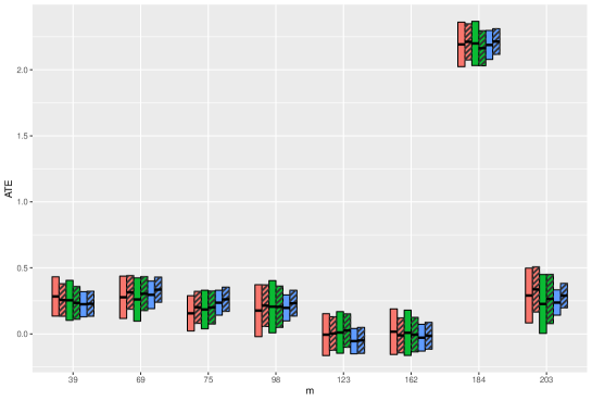
Figure 1: Data analysis: $95\%$ confidence intervals for the ATE of the mutations on the drug resistance to 3TC based on the supervised estimator (8) (undashed bars) and the SS estimator (9) (dashed bars). Here, $m$ is the position of mutation regarded as the treatment indicator. We consider three different combinations to estimate the “propensity score & outcome model” (denoted by the three bar colors): $(\mathrm{i})$ regularized logistic regression & kernel smoothing on the first two directions selected by the regularized sliced inverse regression ( red fill); $(\mathrm{ii})$ regularized logistic regression & regularized parametric regression ( green fill); $(\mathrm{iii})$ random forest & random forest ( blue fill).

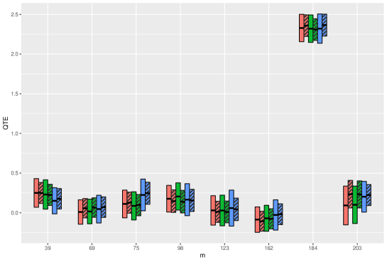
Figure 2: Data analysis: We consider the same scenario as in Figure 1, but now the estimand is the QTE $(\tau=0.5)$.

7 Concluding discussion

We have developed here a family of SS estimators for (a) the ATE and (b) the QTE, in possibly high dimensional settings, and more importantly, we have developed a unified understanding of SS causal inference and its benefits – both in robustness and efficiency – something we feel has been missing in the literature. In addition to the DR property in consistency that can be attained by purely supervised methods as well, we have proved our estimators also possess $n^{1/2}$-consistency and asymptotic normality whenever the propensity score $\pi(\cdot)$ is correctly specified. This property is useful for inference while generally unachievable in supervised settings. Even if this difference in robustness is ignored, our estimators are still guaranteed to be more efficient than their supervised counterparts. Further, as long as all the nuisance functions are correctly specified, our approaches have been shown to attain semi-parametric optimality as well. All our theoretical claims above have also been validated numerically via extensive simulation studies as well as an empirical data analysis.

Further, as a principled and flexible choice for estimating the outcome models in our methods, we have studied thoroughly IPW type kernel smoothing estimators in high dimensional settings with possible use of dimension reduction techniques. We have shown they uniformly converge in probability to $\mathbb{E}(Y\mid\mathbf{P}_{0}^{\rm T}{\mathbf{X}})$ (for the case of the ATE) or $\mathbb{E}\{\psi(Y,\theta)\mid\mathbf{P}_{0}^{\rm T}{\mathbf{X}}\}$ (for the case of the QTE) with some transformation matrix $\mathbf{P}_{0}$, given either the propensity score or the outcome model is correctly specified but not necessarily both. The precise convergence rates have been derived as well. This DR property guarantees the efficiency advantage of our SS methods over their supervised competitors. We view these results also as one of our major contributions. To the best of our knowledge, results of this flavor (especially, in high dimensions, with $p$ diverging) have not been established in the relevant existing literature. They can be applicable to many other problems as well and should therefore be of independent interest.

Extensions

As mentioned in Section 1.1, while we focus on the ATE and QTE for simplicity and clarity of the main messages, our SS methods can be easily extended to other causal estimands, including the general $Z$-estimation problem (Van der Vaart, 2000; Van der Vaart and Wellner, 1996), targeting a parameter defined as the solution to an estimating equation. As long as the estimand has a close form like $\mu_{0}\equiv\mathbb{E}(Y)$, one can construct a family of SS estimators in the same spirit as our ATE estimators (9). An example is the linear regression parameter $\boldsymbol{\beta}_{0}^{\mbox{\tiny LIN}}:=\{\mathbb{E}(\overrightarrow{{\mathbf{X}}}\overrightarrow{{\mathbf{X}}}^{\rm T})\}^{-1}\mathbb{E}(\overrightarrow{{\mathbf{X}}}Y)$, that solves the equation: $\mathbb{E}\{\overrightarrow{{\mathbf{X}}}(Y-\overrightarrow{{\mathbf{X}}}^{\rm T}\boldsymbol{\beta}_{0}^{\mbox{\tiny LIN}})\}={\mathbf{0}}_{d}$, where $\overrightarrow{{\mathbf{X}}}:=(1,{\mathbf{X}}^{\rm T})^{\rm T}$. On the other hand, for estimating equations that cannot be solved straightforwardly, the one-step update strategy, used for our QTE estimators (30), allows for simple and flexible implementations of SS estimation and inference with various choices of nuisance estimators. For instance, our approach to constructing the SS QTE estimators can be adapted for the quantile regression parameter $\boldsymbol{\beta}_{0}^{\mbox{\tiny QUAN}}$, defined by the equation $\mathbb{E}[\overrightarrow{{\mathbf{X}}}\{I(Y<\overrightarrow{{\mathbf{X}}}^{\rm T}\boldsymbol{\beta}_{0}^{\mbox{\tiny QUAN}})-\tau\}]={\mathbf{0}}_{d}$, with extra technical effort. These SS estimators for the general estimating equation problems are expected to possess desirable properties, such as improved robustness and efficiency relative to their supervised counterparts, which are similar in spirit to those stated in Sections 2 and 3 for our SS ATE and QTE estimators. We will briefly discuss in Appendix A the methodological details of these possible extensions of our SS inference methods to the general $Z$-estimation problem under the potential outcome framework. However, a detailed theoretical analysis is beyond the scope (and primary goals) of the current work, and therefore, we choose not to delve any further into these aspects here.

Lastly, in this article, we have only considered cases where the labeled and unlabeled data are equally distributed and thereby satisfy Assumption 1.1. However, the labeling mechanisms in some practical problems are in fact not determined by design and hence, labeling bias can exist between $\mathcal{L}$ and $\mathcal{U}$. It is important to note that, due to the disproportion assumption (1), one cannot simply analyze such settings by using classical missing data theory (Tsiatis, 2007; Little and Rubin, 2019), which requires the proportion of complete observations is bounded away from zero in the sample. Some recent attention has been paid to SS inference with labeling bias in the context of linear regression (Chakrabortty and Cai, 2018, Section II) and mean estimation (Zhang, Chakrabortty and Bradic, 2021). For treatment effect estimation, which is more technically complicated owing to the potential outcome framework, a primary challenge is that there exists no consistent supervised method when the labeled and unlabeled data follow different distributions; so the goal of using unlabeled data to ‘improve’ estimation accuracy compared to supervised approaches becomes somewhat ambiguous. With biased labeling mechanisms, we believe SS inference for treatment effect needs to be studied under a novel framework and thus poses an interesting problem for future research.

Appendix A Extension to general $Z$-estimation problems

In this section, we briefly discuss the SS inference strategy for the general $Z$-estimation problem (Van der Vaart and Wellner, 1996; Van der Vaart, 2000) under the potential outcome framework, based on a natural extension of our proposed methods for the ATE and the QTE in Sections 2 and 3. Specifically, for some fixed $d\geq 1$, we are interested in a $d$-dimensional parameter $\boldsymbol{\theta}_{0}\in\Lambda\subset\mathbb{R}^{d}$, for some $\Lambda$, defined as the solution to the estimating equation:

$$\mathbb{E}\{\boldsymbol{\psi}(Y,{\mathbf{X}},\boldsymbol{\theta}_{0})\}~{}=~{}{\mathbf{0}}_{d},$$ (56)

where $\boldsymbol{\psi}(\cdot,\cdot,\cdot)\in\mathbb{R}^{d}$ is some known function that satisfies: $\mathbb{E}\{\|\boldsymbol{\psi}(Y,{\mathbf{X}},\boldsymbol{\theta})\|^{2}\}<\infty$ for any $\boldsymbol{\theta}\in\Lambda$, and that $\mathbf{H}(\boldsymbol{\theta}):=\partial\mathbb{E}\{\boldsymbol{\psi}(Y,{\mathbf{X}},\boldsymbol{\theta})\}/\partial\boldsymbol{\theta}$ exists and is non-singular in a neighborhood $\mathcal{B}(\boldsymbol{\theta}_{0},\varepsilon)$ of $\boldsymbol{\theta}_{0}$ for some $\varepsilon>0$. In particular, the special cases with $\boldsymbol{\psi}(Y,{\mathbf{X}},\boldsymbol{\theta})\equiv Y-\boldsymbol{\theta}$ and $\boldsymbol{\psi}(Y,{\mathbf{X}},\boldsymbol{\theta})\equiv I(Y<\boldsymbol{\theta})-\tau$, with $d=1$, correspond to the earlier cases of the ATE and the QTE, respectively. This type of SS $Z$-estimation problems (56) – but without the missingness of the potential outcome $Y$ in the labeled data, which can be viewed as a special case of the following discussion with $T\equiv 1$, has been studied in Chapter 2 of Chakrabortty (2016).

SS estimators

Similar in spirit to (26), we know that the following DR type representation:

$${\mathbf{0}}_{d} ~{}=~{} \mathbb{E}\{\boldsymbol{\psi}(Y,{\mathbf{X}},\boldsymbol{\theta}_{0})\}$$

$$~{}=~{} \mathbb{E}\{\boldsymbol{\phi}^{*}({\mathbf{X}},\boldsymbol{\theta}_{0})\}+\mathbb{E}[\{\pi^{*}({\mathbf{X}})\}^{-1}T\{\boldsymbol{\psi}(Y,{\mathbf{X}},\boldsymbol{\theta}_{0})-\boldsymbol{\phi}^{*}({\mathbf{X}},\boldsymbol{\theta}_{0})\}],$$

with arbitrary functions $\{\pi^{*}(\cdot),\boldsymbol{\phi}^{*}(\cdot,\cdot)\}$, holds true for the estimating equation (56), as long as either $\pi^{*}({\mathbf{X}})=\pi({\mathbf{X}})$ or $\boldsymbol{\phi}^{*}({\mathbf{X}},\boldsymbol{\theta})=\boldsymbol{\phi}({\mathbf{X}},\boldsymbol{\theta}):=\mathbb{E}\{\boldsymbol{\psi}(Y,{\mathbf{X}},\boldsymbol{\theta})\mid{\mathbf{X}}\}$, but not necessarily both. The empirical version of (A) constructed based on $\mathcal{L}\cup\mathcal{U}$ is then given by:

$$\mathbb{E}_{n+N}\{\widehat{\boldsymbol{\phi}}_{n}({\mathbf{X}},\boldsymbol{\theta})\}+\mathbb{E}_{n}[\{\widehat{\pi}_{N}({\mathbf{X}})\}^{-1}T\{\boldsymbol{\psi}(Y,{\mathbf{X}},\boldsymbol{\theta})-\widehat{\boldsymbol{\phi}}_{n}({\mathbf{X}},\boldsymbol{\theta})\}]~{}=~{}{\mathbf{0}}_{d},$$ (58)

where $\widehat{\boldsymbol{\phi}}_{n}(\cdot,\cdot)$ is some estimator of $\boldsymbol{\phi}^{*}(\cdot,\cdot)$ from $\mathcal{L}$, constructed via the cross-fitting procedures similar to (31)–(32) so that ${\mathbf{X}}_{i}$ and $\widehat{\boldsymbol{\phi}}_{n}(\cdot,\cdot)$ are independent in $\widehat{\boldsymbol{\phi}}_{n}({\mathbf{X}}_{i},\boldsymbol{\theta})$ $(i=1,\ldots,n)$, and $\widehat{\pi}_{N}(\cdot)$ is some estimator of $\pi(\cdot)$ based on $\mathcal{U}$, same as in Sections 2–3 before. Then, following derivations analogous to those at the beginning of Section 3.1, which yielded our SS QTE estimators (30), we can implement the one-step update approach based on the influence function corresponding to (58), and obtain a family of semi-supervised $Z$-estimators for $\boldsymbol{\theta}_{0}$:

$$\quad\widehat{\boldsymbol{\theta}}_{\mbox{\tiny SS}}~{}:=~{}\widehat{\boldsymbol{\theta}}_{\mbox{\tiny INIT}}+\{\widehat{\mathbf{H}}_{n}(\widehat{\boldsymbol{\theta}}_{\mbox{\tiny INIT}})\}^{-1}(\mathbb{E}_{n}[\{\widehat{\pi}_{N}({\mathbf{X}})\}^{-1}T\{\widehat{\boldsymbol{\phi}}_{n}({\mathbf{X}},\widehat{\boldsymbol{\theta}}_{\mbox{\tiny INIT}})-\boldsymbol{\psi}(Y,{\mathbf{X}},\widehat{\boldsymbol{\theta}}_{\mbox{\tiny INIT}})\}]-$$ (59)

$$\phantom{\quad\widehat{\boldsymbol{\theta}}_{\mbox{\tiny SS}}~{}:=~{}\widehat{\boldsymbol{\theta}}_{\mbox{\tiny INIT}}+\{\widehat{\mathbf{H}}_{n}(\widehat{\boldsymbol{\theta}}_{\mbox{\tiny INIT}})\}^{-1}(}\mathbb{E}_{n+N}\{\widehat{\boldsymbol{\phi}}_{n}({\mathbf{X}},\widehat{\boldsymbol{\theta}}_{\mbox{\tiny INIT}})\}),$$

indexed by $\{\widehat{\pi}_{N}(\cdot),\widehat{\boldsymbol{\phi}}_{n}(\cdot,\cdot),\widehat{\boldsymbol{\theta}}_{\mbox{\tiny INIT}},\widehat{\mathbf{H}}_{n}(\cdot)\}$, where $\widehat{\boldsymbol{\theta}}_{\mbox{\tiny INIT}}$ is an initial estimator of $\boldsymbol{\theta}_{0}$ and $\widehat{\mathbf{H}}_{n}(\cdot)$ is an estimator of $\mathbf{H}(\cdot)$, both based on $\mathcal{L}$. Of course, if the analytical solution, with respect to $\boldsymbol{\theta}$, of (58) exists, one can directly take it as the SS estimator $\widehat{\boldsymbol{\theta}}_{\mbox{\tiny SS}}$ itself. Our SS ATE estimators $\widehat{\mu}_{\mbox{\tiny SS}}$, given in (9), are examples of this type. However, the one-step update (59) is obviously a more general strategy that is implementation-friendly and is broadly applicable to estimating equations of various forms, regardless of whether their analytical solutions exist or not.

Properties of $\widehat{\boldsymbol{\theta}}_{\mbox{\tiny SS}}$ (brief sketch)

To derive the properties of our SS estimators $\widehat{\boldsymbol{\theta}}_{\mbox{\tiny SS}}$, we need to impose the following restrictions on the complexity of the class of the estimating functions:

For some $$\varepsilon>0 \{\boldsymbol{\psi}(Y,{\mathbf{X}},\boldsymbol{\theta}):\boldsymbol{\theta}\in\mathcal{B}(\boldsymbol{\theta}_{0},\varepsilon)\}$$, the (random) function class (60)

lies in a $${\mathbb{P}}$$-Donsker class with square integrable envelope functions,  and

$$\mathbb{E}_{\mathbf{Z}}\{\|\boldsymbol{\psi}(Y,{\mathbf{X}},\widetilde{\boldsymbol{\theta}})-\boldsymbol{\psi}(Y,{\mathbf{X}},\boldsymbol{\theta}_{0})\|^{2}\}{\color[rgb]{0,0,0}~{}\xrightarrow{p}~{}}0 \widetilde{\boldsymbol{\theta}}\xrightarrow{p}\boldsymbol{\theta}_{0}$$  for any (random) sequence  .

Further, we require the function $\boldsymbol{\psi}_{0}(\boldsymbol{\theta}):=\mathbb{E}\{\boldsymbol{\psi}(Y,{\mathbf{X}},\boldsymbol{\theta})\}$ to be smooth enough so that, in $\mathcal{B}(\boldsymbol{\theta}_{0},\varepsilon)$ for some $\varepsilon>0$, it satisfies the Taylor expansion:

$$\boldsymbol{\psi}_{0}(\boldsymbol{\theta})~{}=~{}\boldsymbol{\psi}_{0}(\boldsymbol{\theta}_{0})+\mathbf{H}(\boldsymbol{\theta}_{0})(\boldsymbol{\theta}-\boldsymbol{\theta}_{0})+{\bf r}(\boldsymbol{\theta},\boldsymbol{\theta}_{0})\hbox{ {\color[rgb]{0,0,0}~{}for} some ${\bf r}(\boldsymbol{\theta},\boldsymbol{\theta}_{0})${\color[rgb]{0,0,0},}}$$ (61)

such that $$\|{\bf r}(\boldsymbol{\theta},\boldsymbol{\theta}_{0})\|{\color[rgb]{0,0,0}~{}=~{}}O(\|\boldsymbol{\theta}-\boldsymbol{\theta}_{0}\|^{2}) \boldsymbol{\theta}\to\boldsymbol{\theta}_{0}$$  as  .

These conditions (60)–(61) are fairly mild and standard for estimating equation problems, while their analogues can be found in the (supervised) $Z$-estimation literature such as Van der Vaart (2000). It is also noteworthy that, under the basic Assumption 3.1, (60)–(61) are in fact satisfied by the special case $\boldsymbol{\psi}(Y,{\mathbf{X}},\boldsymbol{\theta})\equiv I(Y<\boldsymbol{\theta})-\tau$ with $d=1$, which is the estimating function corresponding to the QTE; see the proof of Theorem 3.1 in Section B.7 for details.

Further, we need to regulate the behavior of the components $\{\widehat{\pi}_{N}(\cdot),\widehat{\boldsymbol{\phi}}_{n}(\cdot,\cdot),\widehat{\boldsymbol{\theta}}_{\mbox{\tiny INIT}},\widehat{\mathbf{H}}_{n}(\cdot)\}$ in (59) and the possibly misspecified limits $\{\pi^{*}(\cdot),\boldsymbol{\phi}^{*}(\cdot,\cdot)\}$ of $\{\widehat{\pi}_{N}^{*}(\cdot),\widehat{\boldsymbol{\phi}}_{n}^{*}(\cdot,\cdot)\}$. Noticing that the high-level conditions on $\{\widehat{\pi}_{N}(\cdot),\widehat{\phi}_{n}(\cdot,\cdot),\widehat{\theta}_{\mbox{\tiny INIT}},\widehat{f}_{n}(\cdot),\pi^{*}(\cdot),\phi^{*}(\cdot,\cdot)\}$ that were enlisted in Assumptions 3.2–3.5, do not require any specific forms of these components, we can easily adapt them for the case of the general estimating equation (56), with appropriate modifications for the (fixed-dimensional) vector/matrix-valued (random) functions involved, e.g., taking the column-wise $L_{2}$-norms $\|\cdot\|$ of these functions and their moments; see the definition of $\|\cdot\|$ in the Notation paragraph at the beginning of Section 2.

Under the above assumptions on the estimating functions and the nuisance components, as well as some necessary (and fairly reasonable) convergence rate conditions, we can show the following results for our SS estimators $\widehat{\boldsymbol{\theta}}_{\mbox{\tiny SS}}$, which are similar in flavor to those established for our SS ATE and QTE estimators in Sections 2–3.

1. Double robustness: Whenever either $\pi^{*}(\cdot)=\pi(\cdot)$ or $\boldsymbol{\phi}^{*}(\cdot,\cdot)=\boldsymbol{\phi}(\cdot,\cdot)$ holds, but not necessarily both, our SS estimators $\widehat{\boldsymbol{\theta}}_{\mbox{\tiny SS}}$ is consistent for $\boldsymbol{\theta}_{0}$.

2. $n^{1/2}$ consistency and asymptotic normality: Suppose that $\pi^{*}(\cdot)=\pi(\cdot)$. Then, if either $\boldsymbol{\phi}^{*}(\cdot,\cdot)=\boldsymbol{\phi}(\cdot,\cdot)$ or we can use the massive unlabeled data to estimate $\pi(\cdot)$ at a rate faster than $n^{-1/2}$, but not necessarily both, our estimators $\widehat{\boldsymbol{\theta}}_{\mbox{\tiny SS}}$ has the following expansion:

   $$\widehat{\boldsymbol{\theta}}_{\mbox{\tiny SS}}-\boldsymbol{\theta}_{0}~{}=~{}n^{-1}\hbox{$\sum_{i=1}^{n}$}\boldsymbol{\omega}_{\mbox{\tiny SS}}({\mathbf{Z}}_{i},\boldsymbol{\theta}_{0})+o_{p}(n^{-1/2}),\hbox{ with }\boldsymbol{\omega}_{\mbox{\tiny SS}}({\mathbf{Z}},\boldsymbol{\theta}_{0}):=$$ (62)

   $$\{\mathbf{H}(\boldsymbol{\theta}_{0})\}^{-1}[\{\pi({\mathbf{X}})\}^{-1}T\{\boldsymbol{\phi}^{*}({\mathbf{X}},\boldsymbol{\theta}_{0})-\boldsymbol{\psi}(Y,{\mathbf{X}},\boldsymbol{\theta}_{0})\}-\mathbb{E}\{\boldsymbol{\phi}^{*}({\mathbf{X}},\boldsymbol{\theta}_{0})\}],$$

   for an arbitrary $\boldsymbol{\phi}^{*}(\cdot,\cdot)$, not necessarily equal to $\boldsymbol{\phi}(\cdot,\cdot)$. This property is generally unachievable in purely supervised settings (similar in spirit to our discussions in Remarks 2.2 and 3.4). Further, the expansion (62) implies the limiting distribution of $\widehat{\boldsymbol{\theta}}_{\mbox{\tiny SS}}$, given by:

   $$n^{1/2}(\widehat{\boldsymbol{\theta}}_{\mbox{\tiny SS}}-\boldsymbol{\theta}_{0})~{}\xrightarrow{d}~{}\mathcal{N}_{d}[\,{\mathbf{0}}_{d},\hbox{cov}\{\boldsymbol{\omega}_{\mbox{\tiny SS}}({\mathbf{Z}},\boldsymbol{\theta}_{0})\}\,]\quad(n,N\to\infty).$$

3. Efficiency improvement and optimality: Setting aside the difference in robustness from our SS estimators, as stated in (ii), the best achievable influence function of a supervised estimator for $\boldsymbol{\theta}_{0}$, with the same outcome model estimator $\widehat{\boldsymbol{\phi}}_{n}(\cdot,\cdot)$, is given by:

   $$\boldsymbol{\omega}_{\mbox{\tiny SUP}}({\mathbf{Z}},\boldsymbol{\theta}_{0})~{}:=~{}\{\mathbf{H}(\boldsymbol{\theta}_{0})\}^{-1}[\{\pi({\mathbf{X}})\}^{-1}T\{\boldsymbol{\phi}^{*}({\mathbf{X}},\boldsymbol{\theta}_{0})-\boldsymbol{\psi}(Y,{\mathbf{X}},\boldsymbol{\theta}_{0})\}-\boldsymbol{\phi}^{*}({\mathbf{X}},\boldsymbol{\theta}_{0})].$$

   Comparing the supervised and semi-supervised asymptotic covariance matrices, when $\boldsymbol{\phi}^{*}({\mathbf{X}},\boldsymbol{\theta})\equiv\mathbb{E}\{\boldsymbol{\psi}(Y,{\mathbf{X}},\boldsymbol{\theta})\mid{\bf g}({\mathbf{X}})\}$ for some function ${\bf g}(\cdot)$, we notice that

   $$\hbox{cov}\{\boldsymbol{\omega}_{\mbox{\tiny SUP}}({\mathbf{Z}},\boldsymbol{\theta}_{0})\}-\hbox{cov}\{\boldsymbol{\omega}_{\mbox{\tiny SS}}({\mathbf{Z}},\boldsymbol{\theta}_{0})\}~{}=~{}\{\mathbf{H}(\boldsymbol{\theta}_{0})\}^{-1}\hbox{cov}\{\boldsymbol{\phi}^{*}({\mathbf{X}},\boldsymbol{\theta}_{0})\}\{\mathbf{H}(\boldsymbol{\theta}_{0})\}^{-1},$$

   which is positive semi-definite. This indicates the efficiency superiority of our SS estimators over their supervised counterparts. Moreover, as long as both the propensity score $\pi(\cdot)$ and the outcome model $\boldsymbol{\phi}(\cdot,\cdot)$ are correctly specified, the SS estimator’s influence function $\boldsymbol{\omega}_{\mbox{\tiny SS}}({\mathbf{Z}},\boldsymbol{\theta}_{0})$, given in (62), actually equals the efficient influence function for estimating $\boldsymbol{\theta}_{0}$ under the semi-parametric model (22), thus implying that $\widehat{\boldsymbol{\theta}}_{\mbox{\tiny SS}}$ attains the corresponding semi-parametric efficiency bound and is (locally) semi-parametric efficient.

Appendix B Technical details

B.1 Preliminary lemmas

The following Lemma B.1 would be useful in the proofs of the main theorems, in particular, the results in Section 3 regarding QTE estimation.

Lemma B.1.

Suppose there are two independent samples, $\mathcal{S}_{1}$ and $\mathcal{S}_{2}$, consisting of $n$ and $m$ independent copies of $({\mathbf{X}}^{\rm T},Y)^{\rm T}$, respectively. For $\mbox{\boldmath$\gamma$}\in\mathbb{R}^{d}$ with some fixed $d$, let $\widehat{g}_{n}({\mathbf{x}},\mbox{\boldmath$\gamma$})$ be an estimator of a measurable function $g({\mathbf{x}},\mbox{\boldmath$\gamma$})\in\mathbb{R}$ based on $\mathcal{S}_{1}$ and define:

$$\mathbb{G}_{m}\{\widehat{g}_{n}({\mathbf{X}},\mbox{\boldmath$\gamma$})\}~{}:=~{}m^{1/2}[m^{-1}\hbox{$\sum_{({\mathbf{X}}_{i}^{\rm T},Y_{i})^{\rm T}\in\mathcal{S}_{2}}$}\widehat{g}_{n}({\mathbf{X}}_{i},\mbox{\boldmath$\gamma$})-\mathbb{E}_{\mathbf{X}}\{\widehat{g}_{n}({\mathbf{X}},\mbox{\boldmath$\gamma$})\}].$$

For some set $\mathcal{T}\subset\mathbb{R}^{d}$, denote

$$\Delta(\mathcal{S}_{1})~{}:=~{}(\hbox{$\sup_{\mbox{\boldmath$\gamma$}\in\mathcal{T}}$}\mathbb{E}_{\mathbf{X}}[\{\widehat{g}_{n}({\mathbf{X}},\mbox{\boldmath$\gamma$})\}^{2}])^{1/2},\ M(\mathcal{S}_{1}):=\hbox{$\sup_{{\mathbf{x}}\in{\cal X},\,\mbox{\boldmath$\gamma$}\in\mathcal{T}}$}|\widehat{g}_{n}({\mathbf{x}},\mbox{\boldmath$\gamma$})|.$$

For any $\eta\in(0,\Delta(\mathcal{S}_{1})+c\,]$, suppose ${\cal G}_{n}:=\{\widehat{g}_{n}({\mathbf{X}},\mbox{\boldmath$\gamma$}):\mbox{\boldmath$\gamma$}\in\mathcal{T}\}$ satisfies that

$$N_{[\,]}\{\eta,{\cal G}_{n}\mid\mathcal{S}_{1},L_{2}({\mathbb{P}}_{\mathbf{X}})\}~{}\leq~{}H(\mathcal{S}_{1})\eta^{-c}{\color[rgb]{0,0,0},}$$ (63)

with some function $H(\mathcal{S}_{1})>0$. Here ${\cal G}_{n}$ is indexed by $\gamma$ only and treats $\widehat{g}_{n}(\cdot,\mbox{\boldmath$\gamma$})$ as a nonrandom function. Assume $H(\mathcal{S}_{1})=O_{p}(a_{n})$, $\Delta(\mathcal{S}_{1})=O_{p}(d_{n,2})$ and $M(\mathcal{S}_{1})=O_{p}(d_{n,\infty})$ with some positive sequences $a_{n}$, $d_{n,2}$ and $d_{n,\infty}$ allowed to diverge, then we have:

$$\hbox{$\sup_{\mbox{\boldmath$\gamma$}\in\mathcal{T}}$}|\mathbb{G}_{m}\{\widehat{g}_{n}({\mathbf{X}},\mbox{\boldmath$\gamma$})\}|~{}=~{}O_{p}(r_{n,m}),$$

where $r_{n,m}=d_{n,2}\{\hbox{log}\,a_{n}+\hbox{log}\,(d_{n,2}^{-1})\}+m^{-1/2}d_{n,\infty}\{(\hbox{log}\,a_{n})^{2}+(\hbox{log}\,d_{n,2})^{2}\}$.

B.2 Proof of Lemma B.1

For any $\delta\in(0,\Delta(\mathcal{S}_{1})+c\,]$, we have that the bracketing integral

$$J_{[\,]}\{\delta,{\cal G}_{n}\mid\mathcal{S}_{1},L_{2}({\mathbb{P}}_{\mathbf{X}})\} ~{}\equiv~{} \hbox{$\int_{0}^{\delta}$}[1+\hbox{log}\,N_{[\,]}\{\eta,{\cal G}_{n}\mid\mathcal{S}_{1},L_{2}({\mathbb{P}}_{\mathbf{X}})\}]^{1/2}d\eta$$

$$~{}\leq~{} \hbox{$\int_{0}^{\delta}$}1+\hbox{log}\,N_{[\,]}\{\eta,{\cal G}_{n}\mid\mathcal{S}_{1},L_{2}({\mathbb{P}}_{\mathbf{X}})\}d\eta$$

$$~{}\leq~{} \hbox{$\int_{0}^{\delta}$}1+\hbox{log}\,H(\mathcal{S}_{1})-c\,\hbox{log}\,\eta\,d\eta$$

$$~{}=~{} \delta\{1+\hbox{log}\,H(\mathcal{S}_{1})\}+c\,(\delta-\delta\,\hbox{log}\,\delta),$$

where the third step is due to (63). This, combined with Lemma 19.36 of Van der Vaart (2000), implies:

$$\phantom{~{}=~{}}\mathbb{E}_{\mathbf{X}}[\hbox{$\sup_{\mbox{\boldmath$\gamma$}\in\mathcal{T}}$}|\mathbb{G}_{m}\{\widehat{g}_{n}({\mathbf{X}},\mbox{\boldmath$\gamma$})\}|]$$

$$~{}\leq~{}J_{[\,]}\{\delta,{\cal G}_{n}\mid\mathcal{S}_{1},L_{2}({\mathbb{P}}_{\mathbf{X}})\}+[J_{[\,]}\{\delta,{\cal G}_{n}\mid\mathcal{S}_{1},L_{2}({\mathbb{P}}_{\mathbf{X}})\}]^{2}M(\mathcal{S}_{1})\delta^{-2}m^{-1/2}$$

$$~{}\leq~{}\delta\{1+\hbox{log}\,H(\mathcal{S}_{1})\}+c\,(\delta-\delta\,\hbox{log}\,\delta)+\{1+\hbox{log}\,H(\mathcal{S}_{1})+c\,(1-\hbox{log}\,\delta)\}^{2}M(\mathcal{S}_{1})m^{-1/2}$$

for any $\delta\in(\Delta(\mathcal{S}_{1}),\Delta(\mathcal{S}_{1})+c\,]$. Therefore,

$$\mathbb{E}_{\mathbf{X}}[\hbox{$\sup_{\mbox{\boldmath$\gamma$}\in\mathcal{T}}$}|\mathbb{G}_{m}\{\widehat{g}_{n}({\mathbf{X}},\mbox{\boldmath$\gamma$})\}|] ~{}\leq~{} \Delta(\mathcal{S}_{1})\{1+\hbox{log}\,H(\mathcal{S}_{1})\}+c\,\{\Delta(\mathcal{S}_{1})-\Delta(\mathcal{S}_{1})\,\hbox{log}\,\Delta(\mathcal{S}_{1})\}+$$

$$~{}~{}[1+\hbox{log}\,H(\mathcal{S}_{1})+c\,\{1-\hbox{log}\,\Delta(\mathcal{S}_{1})\}]^{2}M(\mathcal{S}_{1})m^{-1/2}.$$

Since the right hand side in the above is $O_{p}(r_{n,m})$, it gives that

$$\mathbb{E}_{\mathbf{X}}[\hbox{$\sup_{\mbox{\boldmath$\gamma$}\in\mathcal{T}}$}|\mathbb{G}_{m}\{\widehat{g}_{n}({\mathbf{X}},\mbox{\boldmath$\gamma$})\}|]~{}=~{}O_{p}(r_{n,m}).$$ (64)

Then, for any positive sequence $t_{n}\to\infty$, we have

$$\phantom{=}{\mathbb{P}}_{\mathcal{S}_{2}}[\hbox{$\sup_{\mbox{\boldmath$\gamma$}\in\mathcal{T}}$}|\mathbb{G}_{m}\{\widehat{g}_{n}({\mathbf{X}},\mbox{\boldmath$\gamma$})\}|>t_{n}r_{n,m}\mid\mathcal{S}_{1}]$$

$$~{}\leq~{}(t_{n}r_{n,m})^{-1}\mathbb{E}_{\mathbf{X}}[\hbox{$\sup_{\mbox{\boldmath$\gamma$}\in\mathcal{T}}$}|\mathbb{G}_{m}\{\widehat{g}_{n}({\mathbf{X}},\mbox{\boldmath$\gamma$})\}|]~{}=~{}o_{p}(1),$$

where the first step holds by Markov’s inequality and the last step is due to (64). This, combined with Lemma 6.1 of Chernozhukov et al. (2018), gives that

$${\mathbb{P}}[\hbox{$\sup_{\mbox{\boldmath$\gamma$}\in\mathcal{T}}$}|\mathbb{G}_{m}\{\widehat{g}_{n}({\mathbf{X}},\mbox{\boldmath$\gamma$})\}|>t_{n}r_{n,m}]~{}\to~{}0,$$

which completes the proof.

B.3 Proof of Theorem 2.1

Denote $\mathbb{E}_{n,k}^{*}\{\widehat{g}({\mathbf{Z}})\}:=n_{\mathbb{K}}^{-1}\sum_{i\in{\cal I}_{k}}\widehat{g}({\mathbf{Z}}_{i})$ for any random function $\widehat{g}(\cdot)$ $(k=1,\ldots,\mathbb{K})$. Write

$$\widehat{\mu}_{\mbox{\tiny SS}}-\mu_{0}~{}=~{}S_{1}+S_{2}+S_{3}+S_{4}+S_{5},$$ (65)

where

$$S_{1} ~{}:=~{} \mathbb{E}_{n}[\{\pi^{*}({\mathbf{X}})\}^{-1}T\{Y-m^{*}({\mathbf{X}})\}]+\mathbb{E}_{n+N}\{m^{*}({\mathbf{X}})\}-\mu_{0},$$ (66)

$$S_{2} ~{}:=~{} \mathbb{E}_{n}([\nu_{n,N}-\{\pi^{*}({\mathbf{X}})\}^{-1}T]\{\widehat{m}_{n}({\mathbf{X}})-m^{*}({\mathbf{X}})\})=\mathbb{K}^{-1}\hbox{$\sum_{k=1}^{\mathbb{K}}$}S_{2,k}$$

$$~{}:=~{} \mathbb{K}^{-1}\hbox{$\sum_{k=1}^{\mathbb{K}}$}\mathbb{E}_{n,k}^{*}([\nu_{n,N}-\{\pi^{*}({\mathbf{X}})\}^{-1}T]\{\widehat{m}_{n,k}({\mathbf{X}})-m^{*}({\mathbf{X}})\}),$$

$$S_{3} ~{}:=~{} (1-\nu_{n,N})\mathbb{E}_{N}\{\widehat{m}_{n}({\mathbf{X}})-m^{*}({\mathbf{X}})\}=\mathbb{K}^{-1}\hbox{$\sum_{k=1}^{\mathbb{K}}$}S_{3,k}$$

$$~{}:=~{} \mathbb{K}^{-1}\hbox{$\sum_{k=1}^{\mathbb{K}}$}[(1-\nu_{n,N})\mathbb{E}_{N}\{\widehat{m}_{n,k}({\mathbf{X}})-m^{*}({\mathbf{X}})\}],$$

$$S_{4} ~{}:=~{} \mathbb{E}_{n}[\widehat{D}_{N}({\mathbf{X}})T\{Y-m^{*}({\mathbf{X}})\}],\ S_{5}:=\mathbb{E}_{n}[\widehat{D}_{N}({\mathbf{X}})T\{m^{*}({\mathbf{X}})-\widehat{m}_{n}({\mathbf{X}})\}].$$

We first handle $S_{2}$ and $S_{3}$. To this end, we have:

$$\phantom{~{}=~{}}\mathbb{E}_{\mathbf{Z}}\{([\nu_{n,N}-\{\pi^{*}({\mathbf{X}})\}^{-1}T]\{\widehat{m}_{n,k}({\mathbf{X}})-m^{*}({\mathbf{X}})\})^{2}\}$$

$$~{}\leq~{}c\,\mathbb{E}_{\mathbf{X}}[\{\widehat{m}_{n,k}({\mathbf{X}})-m^{*}({\mathbf{X}})\}^{2}]~{}=~{}O_{p}(w_{n,2}^{2}),$$

where the first step uses the boundedness of $\{\pi^{*}({\mathbf{X}})\}^{-1}$ from Assumption 2.1 and the last step is due to (15) of Assumption 2.2. It now follows that

$$\hbox{var}(S_{2,k}\mid\mathcal{L}_{k}^{-})~{}=~{}O_{p}(n^{-1}w_{n,2}^{2}),\ \hbox{var}(S_{3,k}\mid\mathcal{L}_{k}^{-})~{}=~{}O_{p}(N^{-1}w_{n,2}^{2}).$$

Thus, Chebyshev’s inequality gives that, for any positive sequence $t_{n}\to\infty$,

$${\mathbb{P}}_{\mathcal{L}_{k}}(|S_{2,k}-\mathbb{E}_{\mathbf{Z}}(S_{2,k})|\geq t_{n}n^{-1/2}w_{n,2}\mid\mathcal{L}_{k}^{-})~{}\leq~{}n(t_{n}w_{n,2})^{-2}\hbox{var}(S_{2,k}\mid\mathcal{L}_{k}^{-})~{}=~{}o_{p}(1),$$

$${\mathbb{P}}_{\mathcal{U}}(|S_{3,k}-\mathbb{E}_{\mathbf{Z}}(S_{3,k})|\geq t_{n}n^{-1/2}w_{n,2}\mid\mathcal{L}_{k}^{-})~{}\leq~{}n(t_{n}w_{n,2})^{-2}\hbox{var}(S_{3,k}\mid\mathcal{L}_{k}^{-})~{}=~{}o_{p}(1).$$

Then, Lemma 6.1 of Chernozhukov et al. (2018) implies

$$|S_{2,k}-\mathbb{E}_{\mathbf{Z}}(S_{2,k})|~{}=~{}O_{p}(n^{-1/2}w_{n,2}),\ |S_{3,k}-\mathbb{E}_{\mathbf{Z}}(S_{3,k})|~{}=~{}O_{p}(N^{-1/2}w_{n,2}),$$

which gives that

$$|S_{2,k}+S_{3,k}-\mathbb{E}_{\mathbf{Z}}(S_{2,k}+S_{3,k})|~{}=~{}O_{p}(n^{-1/2}w_{n,2}).$$ (67)

In addition, we know that

$$|\mathbb{E}_{\mathbf{Z}}(S_{2,k}+S_{3,k})| ~{}=~{} |\mathbb{E}_{\mathbf{Z}}([1-\{\pi^{*}({\mathbf{X}})\}^{-1}T]\{\widehat{m}_{n,k}({\mathbf{X}})-m^{*}({\mathbf{X}})\})|$$

$$~{}\leq~{} c\,I\{\pi^{*}({\mathbf{X}})\neq\pi({\mathbf{X}})\}\mathbb{E}\{|\widehat{m}_{n,k}({\mathbf{X}})-m^{*}({\mathbf{X}})|\}$$

$$~{}=~{} I\{\pi^{*}({\mathbf{X}})\neq\pi({\mathbf{X}})\}O_{p}(w_{n,1}),$$

where the second step uses the boundedness of $\{\pi^{*}({\mathbf{X}})\}^{-1}$ from Assumption 2.1 as well as the fact that

$$\mathbb{E}_{\mathbf{Z}}([1-\{\pi({\mathbf{X}})\}^{-1}T]\{\widehat{m}_{n,k}({\mathbf{X}})-m^{*}({\mathbf{X}})\})~{}=~{}0,$$

and the last step holds by (14) of Assumption 2.2. This, combined with (67), gives

$$|S_{2,k}+S_{3,k}|~{}=~{}O_{p}(n^{-1/2}w_{n,2})+I\{\pi^{*}({\mathbf{X}})\neq\pi({\mathbf{X}})\}O_{p}(w_{n,1}),$$

which implies:

$$|S_{2}+S_{3}| ~{}\leq~{} \mathbb{K}^{-1}\hbox{$\sum_{k=1}^{\mathbb{K}}$}|S_{2,k}+S_{3,k}|$$ (68)

$$~{}=~{} O_{p}(n^{-1/2}w_{n,2})+I\{\pi^{*}({\mathbf{X}})\neq\pi({\mathbf{X}})\}O_{p}(w_{n,1}).$$

Next, we control $S_{4}$. We know that

$$\mathbb{E}_{\mathbf{Z}}([\widehat{D}_{N}({\mathbf{X}})T\{Y-m^{*}({\mathbf{X}})\}]^{2})~{}\leq~{}\mathbb{E}_{\mathbf{Z}}([\widehat{D}_{N}({\mathbf{X}})\{Y-m^{*}({\mathbf{X}})\}]^{2})~{}=~{}O_{p}(b_{N}^{2}),$$

where the last step holds by (13) of Assumption 2.1. This implies:

$$\hbox{var}(S_{4}\mid\mathcal{U})~{}=~{}O_{p}(n^{-1}b_{N}^{2}).$$

Thus Chebyshev’s inequality gives that, for any positive sequence $t_{n}\to\infty$,

$${\mathbb{P}}_{\mathcal{L}}(|S_{4}-\mathbb{E}_{\mathbf{Z}}(S_{4})|\geq t_{n}n^{-1/2}b_{N}\mid\mathcal{U})~{}\leq~{}n(t_{n}b_{N})^{-2}\hbox{var}(S_{4}\mid\mathcal{U})~{}=~{}o_{p}(1).$$

Then, by Lemma 6.1 of Chernozhukov et al. (2018), we have

$$|S_{4}-\mathbb{E}_{\mathbf{Z}}(S_{4})|~{}=~{}O_{p}(n^{-1/2}b_{N}).$$ (69)

In addition, if $m^{*}({\mathbf{X}})=m({\mathbf{X}})$, then

$$\mathbb{E}_{\mathbf{Z}}(S_{4})~{}=~{}\mathbb{E}(\mathbb{E}[\widehat{D}_{N}({\mathbf{X}})T\{Y-m({\mathbf{X}})\}\mid\mathcal{U},{\mathbf{X}}]\mid\mathcal{U})~{}=~{}0.$$

Otherwise, we have

$$|\mathbb{E}_{\mathbf{Z}}(S_{4})|~{}\leq~{}(\mathbb{E}_{\mathbf{X}}[\{\widehat{D}_{N}({\mathbf{X}})\}^{2}]\mathbb{E}[\{Y-m^{*}({\mathbf{X}})\}^{2}])^{1/2}~{}=~{}O_{p}(s_{N}),$$

where the first step uses Hölder’s inequality and the last step is due to (12) of Assumption 2.1. Therefore $|\mathbb{E}_{\mathbf{Z}}(S_{4})|=I\{m^{*}({\mathbf{X}})\neq m({\mathbf{X}})\}O_{p}(s_{N})$. This, combined with (69), implies:

$$|S_{4}|~{}=~{}O_{p}(n^{-1/2}b_{N})+I\{m({\mathbf{X}})\neq m^{*}({\mathbf{X}})\}O_{p}(s_{N}).$$ (70)

Now, we consider $S_{5}$. Markov’s inequality gives that, for any positive sequence $t_{n}\to\infty$,

$$\phantom{~{}=~{}}{\mathbb{P}}_{\mathcal{L}}(\mathbb{E}_{n,k}^{*}[\{\widehat{D}_{N}({\mathbf{X}})\}^{2}]\geq t_{n}s_{N}^{2}\mid\mathcal{U})~{}\leq~{}t_{n}^{-1}s_{N}^{-2}\mathbb{E}_{\mathbf{X}}[\{\widehat{D}_{N}({\mathbf{X}})\}^{2}]~{}=~{}o_{p}(1),$$ (71)

$$\phantom{~{}=~{}}{\mathbb{P}}_{\mathcal{L}_{k}}(\mathbb{E}_{n,k}^{*}[\{m^{*}({\mathbf{X}})-\widehat{m}_{n,k}({\mathbf{X}})\}^{2}]\geq t_{n}w_{n,2}^{2}\mid\mathcal{L}_{k}^{-})$$

$$~{}\leq~{}t_{n}^{-1}w_{n,2}^{-2}\mathbb{E}_{\mathbf{X}}[\{m^{*}({\mathbf{X}})-\widehat{m}_{n,k}({\mathbf{X}})\}^{2}]=o_{p}(1)\quad(k=1,\ldots,\mathbb{K}),$$ (72)

where (71) uses (12) of Assumption 2.1 and (72) holds by (15) of Assumption 2.2. Then, by Lemma 6.1 of Chernozhukov et al. (2018), we have

$$\mathbb{E}_{n,k}^{*}[\{\widehat{D}_{N}({\mathbf{X}})\}^{2}]~{}=~{}O_{p}(s_{N}^{2}),$$ (73)

$$\mathbb{E}_{n,k}^{*}[\{m^{*}({\mathbf{X}})-\widehat{m}_{n,k}({\mathbf{X}})\}^{2}]~{}=~{}O_{p}(w_{n,2}^{2})\quad(k=1,\ldots,\mathbb{K}).$$ (74)

Hence, Hölder’s inequality implies:

$$|S_{5}| ~{}\leq~{} \mathbb{K}^{-1}\hbox{$\sum_{k=1}^{\mathbb{K}}$}\mathbb{E}_{n,k}^{*}[|\widehat{D}_{N}({\mathbf{X}})\{m^{*}({\mathbf{X}})-\widehat{m}_{n,k}({\mathbf{X}})\}|]$$ (75)

$$~{}\leq~{} \mathbb{K}^{-1}\hbox{$\sum_{k=1}^{\mathbb{K}}$}(\mathbb{E}_{n,k}^{*}[\{\widehat{D}_{N}({\mathbf{X}})\}^{2}]\mathbb{E}_{n,k}^{*}[\{m^{*}({\mathbf{X}})-\widehat{m}_{n,k}({\mathbf{X}})\}^{2}])^{1/2}=O_{p}(s_{N}\,w_{n,2}),$$

where the last step holds by (73) and(74).

Summing up, the equations (65), (66), (68), (70) and (75) conclude the result.

B.4 Proof of Corollary 2.1

Since $\nu=0$, we have

$$\mathbb{E}_{n+N}\{m^{*}({\mathbf{X}})\}~{}=~{}\mathbb{E}\{m^{*}({\mathbf{X}})\}+O_{p}\{(n+N)^{-1/2}\}~{}=~{}\mathbb{E}\{m^{*}({\mathbf{X}})\}+o_{p}(n^{-1/2}).$$

by the central limit theorem. Then the stochastic expansion directly follows from Theorem 2.1 and the asymptotic normality is obvious.

B.5 Proof of Corollary 2.2

With $\mathbb{E}_{n+N}\{\widehat{m}_{n}({\mathbf{X}})\}$ substituted by $\mathbb{E}_{n}\{\widehat{m}_{n}({\mathbf{X}})\}$, the proof of Theorem 2.1 directly gives the stochastic expansion followed by the asymptotic normality. Then, we have

$$\phantom{~{}=~{}}\hbox{cov}[\{\pi({\mathbf{X}})\}^{-1}T\{Y-m^{*}({\mathbf{X}})\},m^{*}({\mathbf{X}})]$$

$$~{}=~{}\mathbb{E}\{m^{*}({\mathbf{X}})Y\}-\mathbb{E}[\{m^{*}({\mathbf{X}})\}^{2}]-\mathbb{E}\{Y-m^{*}({\mathbf{X}})\}\mathbb{E}\{m^{*}({\mathbf{X}})\}$$

$$~{}=~{}\mathbb{E}\{m^{*}({\mathbf{X}})Y\}-\hbox{var}\{m^{*}({\mathbf{X}})\}.$$

Therefore,

$$\lambda_{\mbox{\tiny SUP}}^{2}~{}=~{}\hbox{var}[\{\pi({\mathbf{X}})\}^{-1}T\{Y-m^{*}({\mathbf{X}})\}]+\hbox{var}\{m^{*}({\mathbf{X}})\}+$$

$$\phantom{\lambda_{\mbox{\tiny SUP}}^{2}=~{}~{}}2\,\hbox{cov}[\{\pi({\mathbf{X}})\}^{-1}T\{Y-m^{*}({\mathbf{X}})\},m^{*}({\mathbf{X}})]$$

$$\phantom{\lambda_{\mbox{\tiny SUP}}^{2}}~{}=~{}\hbox{var}[\{\pi({\mathbf{X}})\}^{-1}T\{Y-m^{*}({\mathbf{X}})\}]-\hbox{var}\{m^{*}({\mathbf{X}})\}+2\,\mathbb{E}\{m^{*}({\mathbf{X}})(Y-\mu_{0})\}.$$

B.6 Proof of Corollary 2.3

The stochastic expansion can be obtained from the proof of Theorem 2.1 with $\widehat{\pi}_{N}(\cdot)$ replaced by $\widehat{\pi}_{n}(\cdot)$. The asymptotic normality directly follows.

B.7 Proof of Theorem 3.1

Write

$$\widehat{\theta}_{\mbox{\tiny SS}}-\theta_{0}~{}=~{}\{T_{1}(\widehat{\theta}_{\mbox{\tiny INIT}})-\theta_{0}\}+\{\widehat{f}_{n}(\widehat{\theta}_{\mbox{\tiny INIT}})\}^{-1}\{T_{2}(\widehat{\theta}_{\mbox{\tiny INIT}})+T_{3}(\widehat{\theta}_{\mbox{\tiny INIT}})+T_{4}(\widehat{\theta}_{\mbox{\tiny INIT}})\},$$ (76)

where

$$T_{1}(\theta) ~{}:=~{} \theta+\{\widehat{f}_{n}(\theta)\}^{-1}(\mathbb{E}_{n}[\{\pi^{*}({\mathbf{X}})\}^{-1}T\{\phi^{*}({\mathbf{X}},\theta)-\psi(Y,\theta)\}]-\mathbb{E}_{n+N}\{\phi^{*}({\mathbf{X}},\theta)\}),$$

$$T_{2}(\theta) ~{}:=~{} \mathbb{E}_{n}([\{\pi^{*}({\mathbf{X}})\}^{-1}T-\nu_{n,N}]\{\widehat{\phi}_{n}({\mathbf{X}},\theta)-\phi^{*}({\mathbf{X}},\theta)\})-$$

$$~{}~{}(1-\nu_{n,N})\mathbb{E}_{N}\{\widehat{\phi}_{n}({\mathbf{X}},\theta)-\phi^{*}({\mathbf{X}},\theta)\},$$

$$T_{3}(\theta) ~{}:=~{} \mathbb{E}_{n}[\widehat{D}_{N}({\mathbf{X}})T\{\phi^{*}({\mathbf{X}},\theta)-\psi(Y,\theta)\}],$$

$$T_{4}(\theta) ~{}:=~{} \mathbb{E}_{n}[\widehat{D}_{N}({\mathbf{X}})T\{\widehat{\phi}_{n}({\mathbf{X}},\theta)-\phi^{*}({\mathbf{X}},\theta)\}].$$

First, the conditions (33) and (34) of Assumption 3.2 give

$${\mathbb{P}}\{\widehat{\theta}_{\mbox{\tiny INIT}}\in\mathcal{B}(\theta_{0},{\varepsilon})\}~{}\to~{}1,$$ (77)

$$\widehat{L}_{n}~{}:=~{}\{\widehat{f}_{n}(\widehat{\theta}_{\mbox{\tiny INIT}})\}^{-1}-\{f(\theta_{0})\}^{-1}~{}=~{}O_{p}(v_{n})~{}=~{}o_{p}(1).$$ (78)

Also, we have

$$\widehat{f}_{n}(\widehat{\theta}_{\mbox{\tiny INIT}})~{}=~{}O_{p}(1){\color[rgb]{0,0,0},}$$ (79)

due to (34) of Assumption 3.2 and the fact that $f(\theta_{0})>0$ from Assumption 3.1.

Now, we consider $T_{1}(\widehat{\theta}_{\mbox{\tiny INIT}})$. According to (33) of Assumption 3.2 and (38) of Assumption 3.4, we have

$$n^{-1/2}\mathbb{G}_{n}[\{\pi^{*}({\mathbf{X}})\}^{-1}T\phi^{*}({\mathbf{X}},\widehat{\theta}_{\mbox{\tiny INIT}})]~{}=~{}n^{-1/2}\mathbb{G}_{n}[\{\pi^{*}({\mathbf{X}})\}^{-1}T\phi^{*}({\mathbf{X}},\theta_{0})]+o_{p}(n^{-1/2}),$$

which implies that

$$\phantom{~{}=~{}}\mathbb{E}_{n}[\{\pi^{*}({\mathbf{X}})\}^{-1}T\phi^{*}({\mathbf{X}},\widehat{\theta}_{\mbox{\tiny INIT}})]$$

$$~{}=~{}\mathbb{E}_{\mathbf{Z}}[\{\pi^{*}({\mathbf{X}})\}^{-1}T\phi^{*}({\mathbf{X}},\widehat{\theta}_{\mbox{\tiny INIT}})]+\mathbb{E}_{n}[\{\pi^{*}({\mathbf{X}})\}^{-1}T\phi^{*}({\mathbf{X}},\theta_{0})]-$$

$$\phantom{~{}=~{}}\mathbb{E}_{\mathbf{Z}}[\{\pi^{*}({\mathbf{X}})\}^{-1}T\phi^{*}({\mathbf{X}},\theta_{0})]+o_{p}(n^{-1/2}).$$ (80)

Considering that $\{\psi(Y,\theta):\theta\in\mathcal{B}(\theta_{0},{\varepsilon})\}$ is a ${\mathbb{P}}$-Donsker class from Theorem 19.3 of Van der Vaart (2000) and the permanence properties of ${\mathbb{P}}$-Donsker classes Van der Vaart and Wellner (1996), Theorem 2.10.6 of Van der Vaart and Wellner (1996) gives that ${\cal D}^{*}=\{\{\pi^{*}({\mathbf{X}})\}^{-1}T\psi(Y,\theta):\theta\in\mathcal{B}(\theta_{0},{\varepsilon})\}$ is ${\mathbb{P}}$-Donsker since $\{\pi^{*}({\mathbf{X}})\}^{-1}T$ and $\psi(Y,\theta)$ are bounded. Moreover, the convergence (77) implies that $\{\pi^{*}({\mathbf{X}})\}^{-1}T\psi(Y,\widehat{\theta}_{\mbox{\tiny INIT}})$ is in ${\cal D}^{*}$ with probability tending to one. In addition, we have

$$\phantom{~{}=~{}}\mathbb{E}_{\mathbf{Z}}[\{\pi^{*}({\mathbf{X}})\}^{-2}T\{\psi(Y,\widehat{\theta}_{\mbox{\tiny INIT}})-\psi(Y,\theta_{0})\}^{2}]$$

$$~{}\leq~{}c\,\mathbb{E}_{\bf Z}[\{I(Y<\widehat{\theta}_{\mbox{\tiny INIT}})-I(Y<\theta_{0})\}^{2}]=c\,F(\widehat{\theta}_{\mbox{\tiny INIT}})+F(\theta_{0})-2F\{\min(\widehat{\theta}_{\mbox{\tiny INIT}},\theta_{0})\}\to 0$$

in probability, because of the boundedness of $\{\pi^{*}({\mathbf{X}})\}^{-2}T$, the continuity of $F(\cdot)$ from Assumption 3.1 and the consistency of $\widehat{\theta}_{\mbox{\tiny INIT}}$ from Assumption 3.2. Hence Lemma 19.24 of Van der Vaart (2000) gives that

$$\mathbb{G}_{n}[\{\pi^{*}({\mathbf{X}})\}^{-1}T\{\psi(Y,\widehat{\theta}_{\mbox{\tiny INIT}})-\psi(Y,\theta_{0})\}]~{}=~{}o_{p}(1),$$

which implies:

$$\mathbb{E}_{n}[\{\pi^{*}({\mathbf{X}})\}^{-1}T\psi(Y,\widehat{\theta}_{\mbox{\tiny INIT}})] ~{}=~{} \mathbb{E}_{\mathbf{Z}}[\{\pi^{*}({\mathbf{X}})\}^{-1}T\psi(Y,\widehat{\theta}_{\mbox{\tiny INIT}})]+\mathbb{E}_{n}[\{\pi^{*}({\mathbf{X}})\}^{-1}T\psi(Y,\theta_{0})]-$$ (81)

$$\mathbb{E}_{\mathbf{Z}}[\{\pi^{*}({\mathbf{X}})\}^{-1}T\psi(Y,\theta_{0})]+o_{p}(n^{-1/2}).$$

Further, the condition (39) gives

$$\mathbb{E}_{n+N}\{\phi^{*}({\mathbf{X}},\widehat{\theta}_{\mbox{\tiny INIT}})\} ~{}=~{} \mathbb{E}_{\mathbf{X}}\{\phi^{*}({\mathbf{X}},\widehat{\theta}_{\mbox{\tiny INIT}})\}+\mathbb{E}_{n+N}\{\phi^{*}({\mathbf{X}},\theta_{0})\}-$$ (82)

$$\mathbb{E}_{\mathbf{X}}\{\phi^{*}({\mathbf{X}},\theta_{0})\}+o_{p}(n^{-1/2}).$$

Since either $\phi^{*}(\cdot,\cdot)=\phi(\cdot,\cdot)$ or $\pi^{*}(\cdot)=\pi(\cdot)$, we know that

$$\mathbb{E}_{\mathbf{Z}}[\{\pi^{*}({\mathbf{X}})\}^{-1}T\{\phi^{*}({\mathbf{X}},\theta_{0})-\psi(Y,\theta_{0})\}]-\mathbb{E}_{\mathbf{X}}\{\phi^{*}({\mathbf{X}},\theta_{0})\}~{}=~{}0,$$ (83)

and that

$$\phantom{~{}=~{}}\mathbb{E}_{\mathbf{Z}}[\{\pi^{*}({\mathbf{X}})\}^{-1}T\{\phi^{*}({\mathbf{X}},\widehat{\theta}_{\mbox{\tiny INIT}})-\psi(Y,\widehat{\theta}_{\mbox{\tiny INIT}})\}]-\mathbb{E}_{\mathbf{X}}\{\phi^{*}({\mathbf{X}},\widehat{\theta}_{\mbox{\tiny INIT}})\}$$

$$~{}=~{}-\mathbb{E}_{\mathbf{Z}}\{\psi(Y,\widehat{\theta}_{\mbox{\tiny INIT}})\}.$$ (84)

In addition, Taylor’s expansion gives that

$$\mathbb{E}_{\bf Z}\{\psi(Y,\widehat{\theta}_{\mbox{\tiny INIT}})\} ~{}=~{} f(\theta_{0})(\widehat{\theta}_{\mbox{\tiny INIT}}-\theta_{0})+O_{p}(|\widehat{\theta}_{\mbox{\tiny INIT}}-\theta_{0}|^{2})$$ (85)

$$~{}=~{} f(\theta_{0})(\widehat{\theta}_{\mbox{\tiny INIT}}-\theta_{0})+O_{p}(u_{n}^{2})$$

$$~{}=~{} O_{p}(u_{n}),$$ (86)

where the residual term in the first step is due to (77) and the fact that $f(\cdot)$ has a bounded derivative in $\mathcal{B}(\theta_{0},{\varepsilon})$ from Assumption 3.1, the second step uses (33) in Assumption 3.2 and the last step holds by the fact that $u_{n}=o(1)$ from Assumption 3.2. Therefore,

$$\mathbb{E}_{n}\{\omega_{n,N}({\mathbf{Z}},\widehat{\theta}_{\mbox{\tiny INIT}})\} ~{}=~{} \mathbb{E}_{n}\{\omega_{n,N}({\mathbf{Z}},\theta_{0})\}-\mathbb{E}_{\mathbf{Z}}\{\psi(Y,\widehat{\theta}_{\mbox{\tiny INIT}})\}+o_{p}(n^{-1/2})$$

$$~{}=~{} \mathbb{E}_{n}\{\omega_{n,N}({\mathbf{Z}},\theta_{0})\}-f(\theta_{0})(\widehat{\theta}_{\mbox{\tiny INIT}}-\theta_{0})+O_{p}(u_{n}^{2})+o_{p}(n^{-1/2})$$

$$~{}=~{} \mathbb{E}_{n}\{\omega_{n,N}({\mathbf{Z}},\theta_{0})\}+O_{p}(u_{n})+o_{p}(n^{-1/2}),$$

where the first step uses (80)–(84), the second step is due to (85) and the last step holds by (86). It now follows that

$$\widehat{L}_{n}\mathbb{E}_{n}\{\omega_{n,N}({\mathbf{Z}},\widehat{\theta}_{\mbox{\tiny INIT}})\}~{}=~{}O_{p}(u_{n}v_{n})+o_{p}(n^{-1/2}){\color[rgb]{0,0,0},}$$ (88)

from (78) and the fact that $\mathbb{E}_{n}\{\omega_{n,N}({\mathbf{Z}},\theta_{0})\}=O_{p}(n^{-1/2})$ from the central limit theorem. Hence, we have

$$T_{1}(\widehat{\theta}_{\mbox{\tiny INIT}})-\theta_{0}~{}=~{}\widehat{\theta}_{\mbox{\tiny INIT}}-\theta_{0}+\{\widehat{f}_{n}(\widehat{\theta}_{\mbox{\tiny INIT}})\}^{-1}\mathbb{E}_{n}\{\omega_{n,N}({\mathbf{Z}},\widehat{\theta}_{\mbox{\tiny INIT}})\}$$

$$\phantom{T_{1}(\widehat{\theta}_{\mbox{\tiny INIT}})-\theta_{0}}~{}=~{}\widehat{\theta}_{\mbox{\tiny INIT}}-\theta_{0}+\{f(\theta_{0})\}^{-1}\mathbb{E}_{n}\{\omega_{n,N}({\mathbf{Z}},\widehat{\theta}_{\mbox{\tiny INIT}})\}+O_{p}(u_{n}v_{n})+o_{p}(n^{-1/2})$$

$$\phantom{T_{1}(\widehat{\theta}_{\mbox{\tiny INIT}})-\theta_{0}}~{}=~{}\widehat{\theta}_{\mbox{\tiny INIT}}-\theta_{0}+\{f(\theta_{0})\}^{-1}[\mathbb{E}_{n}\{\omega_{n,N}({\mathbf{Z}},\theta_{0})\}-f(\theta_{0})(\widehat{\theta}_{\mbox{\tiny INIT}}-\theta_{0})]+$$

$$\phantom{T_{1}(\widehat{\theta}_{\mbox{\tiny INIT}})-\theta_{0}=}O_{p}(u_{n}^{2}+u_{n}v_{n})+o_{p}(n^{-1/2})$$

$$\phantom{T_{1}(\widehat{\theta}_{\mbox{\tiny INIT}})-\theta_{0}}~{}=~{}\{f(\theta_{0})\}^{-1}\mathbb{E}_{n}\{\omega_{n,N}({\mathbf{Z}},\theta_{0})\}+O_{p}(u_{n}v_{n}+u_{n}^{2})+o_{p}(n^{-1/2}),$$ (89)

where the second step uses (88) and the third step is due to (B.7).

Next, we control $T_{2}(\widehat{\theta}_{\mbox{\tiny INIT}})$. Denote

$$\mathcal{P}_{n,k}^{*}~{}:=~{}\{[\{\pi^{*}({\mathbf{X}})\}^{-1}T-\nu_{n,N}]\widehat{\psi}_{n,k}({\mathbf{X}},\theta):\theta\in\mathcal{B}(\theta_{0},{\varepsilon})\}.$$

Due to the boundedness of $[\{\pi^{*}({\mathbf{X}})\}^{-1}T-\nu_{n,N}]$ from Assumption 3.3, we have

$$\phantom{=}N_{[\,]}\{c_{1}\,\eta,\mathcal{P}_{n,k}^{*}\mid\mathcal{L},L_{2}({\mathbb{P}}_{\mathbf{X}})\}~{}\leq~{}N_{[\,]}\{\eta,\mathcal{P}_{n,k}\mid\mathcal{L},L_{2}({\mathbb{P}}_{\mathbf{X}})\}~{}\leq~{}H(\mathcal{L})\eta^{-c},$$ (90)

$$\phantom{~{}=~{}}\hbox{$\sup_{{\mathbf{x}}\in{\cal X},\,\theta\in\mathcal{B}(\theta_{0},{\varepsilon})}$}|[\{\pi^{*}({\mathbf{X}})\}^{-1}T-\nu_{n,N}]\widehat{\psi}_{n,k}({\mathbf{X}},\theta)|$$

$$~{}\leq~{}c\,\hbox{$\sup_{{\mathbf{x}}\in{\cal X},\,\theta\in\mathcal{B}(\theta_{0},{\varepsilon})}$}|\widehat{\psi}_{n,k}({\mathbf{X}},\theta)|=O_{p}(d_{n,\infty}),$$ (91)

$$\phantom{~{}~{}}[\hbox{$\sup_{\theta\in\mathcal{B}(\theta_{0},{\varepsilon})}$}\mathbb{E}_{\mathbf{Z}}\{([\{\pi^{*}({\mathbf{X}})\}^{-1}T-\nu_{n,N}]\widehat{\psi}_{n,k}({\mathbf{X}},\theta))\}^{2}]^{1/2}$$

$$~{}\leq~{}c\,\Delta_{k}(\mathcal{L})=O_{p}(d_{n,2})\quad(k=1,\ldots,\mathbb{K}){\color[rgb]{0,0,0},}$$ (92)

from Assumption 3.5. Then, (90) implies:

$$N_{[\,]}\{\eta,\mathcal{P}_{n,k}^{*}\mid\mathcal{L},L_{2}({\mathbb{P}}_{\mathbf{X}})\}~{}\leq~{}c_{1}^{c_{2}}H(\mathcal{L})\eta^{-c_{2}}.$$ (93)

Since $c_{1}^{c_{2}}H(\mathcal{L})=O_{p}(a_{n})$ from Assumption 3.5, combining (91)–(93) and applying Lemma B.1 yield that

$$\hbox{$\sup_{\theta\in\mathcal{B}(\theta_{0},{\varepsilon})}$}|\mathbb{G}_{n_{\mathbb{K}},k}([\{\pi^{*}({\mathbf{X}})\}^{-1}T-\nu_{n,N}]\widehat{\psi}_{n,k}({\mathbf{X}},\theta))|~{}=~{}O_{p}(r_{n}){\color[rgb]{0,0,0},}$$ (94)

with the notation

$$\mathbb{G}_{n_{\mathbb{K}},k}\{\widehat{g}({\mathbf{Z}})\}~{}:=~{}n_{\mathbb{K}}^{1/2}[n_{\mathbb{K}}^{-1}\hbox{$\sum_{i\in{\cal I}_{k}}$}\widehat{g}({\mathbf{Z}}_{i})-\mathbb{E}_{\mathbf{X}}\{\widehat{g}({\mathbf{Z}})\}]\quad(k=1,\ldots,\mathbb{K}){\color[rgb]{0,0,0},}$$

for any random function $\widehat{g}(\cdot)$. In addition, we have

$$\phantom{=}\hbox{$\sup_{\theta\in\mathcal{B}(\theta_{0},{\varepsilon})}$}|\mathbb{E}_{\mathbf{Z}}([\{\pi^{*}({\mathbf{X}})\}^{-1}T-1]\widehat{\psi}_{n,k}({\mathbf{X}},\theta))|$$

$$~{}\leq~{}c\,I\{\pi^{*}({\mathbf{X}})\neq\pi({\mathbf{X}})\}\hbox{$\sup_{\theta\in\mathcal{B}(\theta_{0},{\varepsilon})}$}\mathbb{E}_{\mathbf{Z}}\{|\widehat{\psi}_{n,k}({\mathbf{X}},\theta)|\}$$

$$~{}=~{}I\{\pi^{*}({\mathbf{X}})\neq\pi({\mathbf{X}})\}O_{p}(d_{n,1}),$$ (95)

where the first step holds by the boundedness of $\{\pi^{*}({\mathbf{X}})\}^{-1}$ from Assumption 3.3 and the fact that

$$\mathbb{E}_{\mathbf{Z}}([\{\pi({\mathbf{X}})\}^{-1}T-1]\widehat{\psi}_{n,k}({\mathbf{X}},\theta))~{}=~{}0,$$

and the last step is due to Assumption 3.5. Moreover, under Assumption 3.5, Lemma B.1 implies that

$$\phantom{~{}=~{}}\hbox{$\sup_{\theta\in\mathcal{B}(\theta_{0},{\varepsilon})}$}|\mathbb{G}_{N}\{\widehat{\psi}_{n,k}({\mathbf{X}},\theta)\}|$$

$$~{}=~{}O_{p}[d_{n,2}\{\hbox{log}\,a_{n}+\hbox{log}\,(d_{n,2}^{-1})\}+N^{-1/2}d_{n,\infty}\{(\hbox{log}\,a_{n})^{2}+(\hbox{log}\,d_{n,2})^{2}\}]$$

$$~{}=~{}O_{p}(r_{n})\quad(k=1,\ldots,\mathbb{K}).$$ (96)

Considering (94)–(96), we know that

$$T_{2}(\widehat{\theta}_{\mbox{\tiny INIT}})~{}=~{}\mathbb{K}^{-1}\hbox{$\sum_{k=1}^{\mathbb{K}}$}\{n_{\mathbb{K}}^{-1/2}\mathbb{G}_{n_{\mathbb{K}},k}([\{\pi^{*}({\mathbf{X}})\}^{-1}T-\nu_{n,N}]\widehat{\psi}_{n,k}({\mathbf{X}},\widehat{\theta}_{\mbox{\tiny INIT}}))-$$

$$\phantom{T_{2}(\widehat{\theta}_{\mbox{\tiny INIT}})=\mathbb{K}^{-1}\hbox{$\sum_{k=1}^{\mathbb{K}}$}\{}N^{-1/2}(1-\nu_{n,N})\mathbb{G}_{N}\{\widehat{\psi}_{n,k}({\mathbf{X}},\widehat{\theta}_{\mbox{\tiny INIT}})\}+$$

$$\phantom{T_{2}(\widehat{\theta}_{\mbox{\tiny INIT}})=\mathbb{K}^{-1}\hbox{$\sum_{k=1}^{\mathbb{K}}$}\{}\mathbb{E}_{\mathbf{Z}}([\{\pi^{*}({\mathbf{X}})\}^{-1}T-1]\widehat{\psi}_{n,k}({\mathbf{X}},\widehat{\theta}_{\mbox{\tiny INIT}}))\}$$

$$\phantom{T_{2}(\widehat{\theta}_{\mbox{\tiny INIT}})}~{}=~{}O_{p}(n^{-1/2}r_{n})+I\{\pi^{*}({\mathbf{X}})\neq\pi({\mathbf{X}})\}O_{p}(d_{n,1}),$$

which, combined with (79), implies that

$$\{\widehat{f}_{n}(\widehat{\theta}_{\mbox{\tiny INIT}})\}^{-1}T_{2}(\widehat{\theta}_{\mbox{\tiny INIT}})~{}=~{}O_{p}(n^{-1/2}r_{n})+I\{\pi^{*}({\mathbf{X}})\neq\pi({\mathbf{X}})\}O_{p}(d_{n,2}).$$ (97)

Further, we now handle $T_{3}(\widehat{\theta}_{\mbox{\tiny INIT}})$. Let $\mathcal{H}_{N}:=\{\widehat{D}_{N}({\mathbf{X}})T\phi^{*}({\mathbf{X}},\theta):\theta\in\mathcal{B}(\theta_{0},{\varepsilon})\}$ and recall $\mathcal{M}=\{\phi^{*}({\mathbf{X}},\theta):\theta\in\mathcal{B}(\theta_{0},{\varepsilon})\}$. We have

$$\phantom{=}N_{[\,]}\{\hbox{$\sup_{{\mathbf{x}}\in{\cal X}}$}|\widehat{D}_{N}({\mathbf{x}})|\eta,\mathcal{H}_{N}\mid\mathcal{U},L_{2}({\mathbb{P}}_{\mathbf{X}})\}~{}\leq~{}N_{[\,]}\{\eta,\mathcal{M},L_{2}({\mathbb{P}}_{\mathbf{X}})\}\leq c_{1}\,\eta^{-c_{2}},$$ (98)

$$\phantom{=}\hbox{$\sup_{{\mathbf{x}}\in{\cal X},\,\theta\in\mathcal{B}(\theta_{0},{\varepsilon})}$}|\widehat{D}_{N}({\mathbf{X}})T\phi^{*}({\mathbf{X}},\theta)|~{}=~{}O_{p}(1),$$ (99)

$$\phantom{=}(\hbox{$\sup_{\theta\in\mathcal{B}(\theta_{0},{\varepsilon})}$}\mathbb{E}_{\mathbf{Z}}[\{\widehat{D}_{N}({\mathbf{X}})T\phi^{*}(Y,\theta)\}^{2}])^{1/2}~{}=~{}O_{p}(s_{N}),$$ (100)

where (98) uses (37) of Assumption 3.4, (99) holds by (36) of Assumption 3.3 and the boundedness of $\phi^{*}({\mathbf{X}},\theta)$ from Assumption 3.4, and (100) is due to (35) of Assumption 3.3 and the boundedness of $\phi^{*}({\mathbf{X}},\theta)$ from Assumption 3.4. Then, (98) gives

$$N_{[\,]}\{\eta,\mathcal{H}_{N}\mid\mathcal{U},L_{2}({\mathbb{P}}_{\mathbf{X}})\}~{}\leq~{}c_{1}\,\{\hbox{$\sup_{{\mathbf{x}}\in{\cal X}}$}|\widehat{D}_{N}({\mathbf{x}})|\}^{c_{2}}\eta^{-c_{2}}.$$ (101)

Since $c_{1}\,\{\hbox{$\sup_{{\mathbf{x}}\in{\cal X}}$}|\widehat{D}_{N}({\mathbf{x}})|\}^{c_{2}}=O_{p}(1)$ from Assumption 3.3, combining (99)–(101) and applying Lemma B.1 yield that

$$\hbox{$\sup_{\theta\in\mathcal{B}(\theta_{0},{\varepsilon})}$}|\mathbb{G}_{n}\{\widehat{D}_{N}({\mathbf{X}})T\phi^{*}(Y,\theta)\}|~{}=~{}O_{p}(z_{n,N}),$$

which gives that

$$|\mathbb{E}_{n}\{\widehat{D}_{N}({\mathbf{X}})T\phi^{*}(Y,\widehat{\theta}_{\mbox{\tiny INIT}})\}-\mathbb{E}_{\mathbf{Z}}\{\widehat{D}_{N}({\mathbf{X}})T\phi^{*}(Y,\widehat{\theta}_{\mbox{\tiny INIT}})\}|~{}=~{}O_{p}(n^{-1/2}z_{n,N}).$$ (102)

Analogously, by Example19.6 of Van der Vaart (2000) and the boundedness of $\psi(Y,\theta)$, we know that

$$|\mathbb{E}_{n}\{\widehat{D}_{N}({\mathbf{X}})T\psi(Y,\widehat{\theta}_{\mbox{\tiny INIT}})\}-\mathbb{E}_{\mathbf{Z}}\{\widehat{D}_{N}({\mathbf{X}})T\psi(Y,\widehat{\theta}_{\mbox{\tiny INIT}})\}|~{}=~{}O_{p}(n^{-1/2}z_{n,N}).$$ (103)

Combining (102) and (103) yields:

$$|T_{3}(\widehat{\theta}_{\mbox{\tiny INIT}})-\mathbb{E}_{\mathbf{Z}}\{T_{3}(\widehat{\theta}_{\mbox{\tiny INIT}})\}|~{}=~{}O_{p}(n^{-1/2}z_{n,N}).$$ (104)

In addition, if $\phi^{*}({\mathbf{X}},\theta)=\phi({\mathbf{X}},\theta)$, then

$$\mathbb{E}_{\mathbf{Z}}\{T_{3}(\widehat{\theta}_{\mbox{\tiny INIT}})\}~{}=~{}\mathbb{E}_{\mathbf{Z}}(\mathbb{E}_{\mathbf{Z}}[\widehat{D}_{N}({\mathbf{X}})T\{\phi^{*}({\mathbf{X}},\widehat{\theta}_{\mbox{\tiny INIT}})-\psi(Y,\widehat{\theta}_{\mbox{\tiny INIT}})\}\mid{\mathbf{X}}])~{}=~{}0.$$

Otherwise, we have

$$|\mathbb{E}_{\mathbf{Z}}\{T_{3}(\widehat{\theta}_{\mbox{\tiny INIT}})\}|~{}\leq~{}(\mathbb{E}_{\mathbf{X}}[\{\widehat{D}_{N}({\mathbf{X}})\}^{2}]\mathbb{E}[\{\phi^{*}({\mathbf{X}},\widehat{\theta}_{\mbox{\tiny INIT}})-\psi(Y,\widehat{\theta}_{\mbox{\tiny INIT}})\}^{2}])^{1/2}~{}=~{}O_{p}(s_{N}),$$

where the last step uses the boundedness of $\phi^{*}({\mathbf{X}},\theta)$ from Assumption 3.4. Hence,

$$|\mathbb{E}_{\mathbf{Z}}\{T_{3}(\widehat{\theta}_{\mbox{\tiny INIT}})\}|~{}=~{}I\{\phi^{*}({\mathbf{X}},\theta)\neq\phi({\mathbf{X}},\theta)\}O_{p}(s_{N}).$$

This, combined with (79) and (104), implies:

$$\{\widehat{f}_{n}(\widehat{\theta}_{\mbox{\tiny INIT}})\}^{-1}T_{3}(\widehat{\theta}_{\mbox{\tiny INIT}})~{}=~{}O_{p}(n^{-1/2}z_{n,N})+I\{\phi^{*}({\mathbf{X}},\theta)\neq\phi({\mathbf{X}},\theta)\}O_{p}(s_{N}).$$ (105)

Eventually, we deal with $T_{4}(\widehat{\theta}_{\mbox{\tiny INIT}})$. Denote

$$\mathcal{Q}_{n,N,k}~{}:=~{}\{\widehat{D}_{N}({\mathbf{X}})T\widehat{\psi}_{n,k}({\mathbf{X}},\theta):\theta\in\mathcal{B}(\theta_{0},{\varepsilon})\}.$$

Due to (36) of Assumption 3.3, we have

$$\phantom{~{}=~{}}N_{[\,]}\{\hbox{$\sup_{{\mathbf{x}}\in{\cal X}}$}|\widehat{D}_{N}({\mathbf{x}})|\eta,\mathcal{Q}_{n,N,k}\mid\mathcal{L}\cup\mathcal{U},L_{2}({\mathbb{P}}_{\mathbf{X}})\}$$

$$~{}\leq~{}N_{[\,]}\{\eta,\mathcal{P}_{n,k}\mid\mathcal{L},L_{2}({\mathbb{P}}_{\mathbf{X}})\}\leq H(\mathcal{L})\eta^{-c},$$ (106)

$$\phantom{~{}=~{}}\hbox{$\sup_{{\mathbf{x}}\in{\cal X},\,\theta\in\mathcal{B}(\theta_{0},{\varepsilon})}$}|\widehat{D}_{N}({\mathbf{X}})\widehat{\psi}_{n,k}({\mathbf{X}},\theta)|$$

$$~{}\leq~{}\hbox{$\sup_{{\mathbf{x}}\in{\cal X}}$}|\widehat{D}_{N}({\mathbf{x}})|\hbox{$\sup_{{\mathbf{x}}\in{\cal X},\,\theta\in\mathcal{B}(\theta_{0},{\varepsilon})}$}|\widehat{\psi}_{n,k}({\mathbf{X}},\theta)|=O_{p}(d_{n,\infty}),$$ (107)

$$\phantom{~{}=~{}}(\hbox{$\sup_{\theta\in\mathcal{B}(\theta_{0},{\varepsilon})}$}\mathbb{E}_{\mathbf{X}}[\{\widehat{D}_{N}({\mathbf{X}})\widehat{\psi}_{n,k}({\mathbf{X}},\theta)\}^{2}])^{1/2}$$

$$~{}\leq~{}\hbox{$\sup_{{\mathbf{x}}\in{\cal X}}$}|\widehat{D}_{N}({\mathbf{x}})|\Delta_{k}(\mathcal{L})=O_{p}(d_{n,2})\quad(k=1,\ldots,\mathbb{K}){\color[rgb]{0,0,0},}$$ (108)

from Assumption 3.5. Then, (106) implies:

$$N_{[\,]}\{\eta,\mathcal{Q}_{n,N,k}\mid\mathcal{L}\cup\mathcal{U},L_{2}({\mathbb{P}}_{\mathbf{X}})\}~{}\leq~{}\{\hbox{$\sup_{{\mathbf{x}}\in{\cal X}}$}|\widehat{D}_{N}({\mathbf{x}})|\}^{c}H(\mathcal{L})\eta^{-c}.$$ (109)

Since $\{\hbox{$\sup_{{\mathbf{x}}\in{\cal X}}$}|\widehat{D}_{N}({\mathbf{x}})|\}^{c}H(\mathcal{L})=O_{p}(a_{n})$ from Assumptions 3.5 and 3.3, combining (107)–(109) and applying Lemma B.1 yield that

$$\hbox{$\sup_{\theta\in\mathcal{B}(\theta_{0},{\varepsilon})}$}|\mathbb{G}_{n_{\mathbb{K}},k}\{\widehat{D}_{N}({\mathbf{X}})\widehat{\psi}_{n,k}({\mathbf{X}},\theta)\}|~{}=~{}O_{p}(r_{n}).$$ (110)

In addition, we have

$$\phantom{~{}=~{}}\hbox{$\sup_{\theta\in\mathcal{B}(\theta_{0},{\varepsilon})}$}|\mathbb{E}_{\mathbf{X}}\{\widehat{D}_{N}({\mathbf{X}})\widehat{\psi}_{n,k}({\mathbf{X}},\theta)\}|$$

$$~{}\leq~{}(\mathbb{E}_{\mathbf{X}}[\{\widehat{D}_{N}({\mathbf{X}})\}^{2}]\hbox{$\sup_{\theta\in\mathcal{B}(\theta_{0},{\varepsilon})}$}\mathbb{E}_{\mathbf{X}}[\{\widehat{\psi}_{n,k}({\mathbf{X}},\theta)\}^{2}])^{1/2}=O_{p}(s_{N}d_{n,2}),$$ (111)

where the first step holds by Hölder’s inequality and the last step is due to Assumptions 3.3 and 3.5. Considering (110) and (111), we know that

$$T_{4}(\widehat{\theta}_{\mbox{\tiny INIT}}) ~{}=~{} \mathbb{K}^{-1}\hbox{$\sum_{k=1}^{\mathbb{K}}$}[n_{\mathbb{K}}^{-1/2}\mathbb{G}_{n_{\mathbb{K}},k}\{\widehat{D}_{N}({\mathbf{X}})\widehat{\psi}_{n,k}({\mathbf{X}},\widehat{\theta}_{\mbox{\tiny INIT}})\}+\mathbb{E}_{\mathbf{X}}\{\widehat{D}_{N}({\mathbf{X}})\widehat{\psi}_{n,k}({\mathbf{X}},\widehat{\theta}_{\mbox{\tiny INIT}})\}]$$

$$~{}=~{} O_{p}(n^{-1/2}r_{n}+s_{N}d_{n,2}),$$

which, combined with (79), implies that

$$\{\widehat{f}_{n}(\widehat{\theta}_{\mbox{\tiny INIT}})\}^{-1}T_{4}(\widehat{\theta}_{\mbox{\tiny INIT}})~{}=~{}O_{p}(n^{-1/2}r_{n}+s_{N}d_{n,2}).$$ (112)

Summing up, the equations (89), (97), (105) and (112) conclude the result.

B.8 Proof of Corollary 3.1

Since $\nu=0$, we have

$$\mathbb{E}_{n+N}\{\phi^{*}({\mathbf{X}},\theta_{0})\}=\mathbb{E}\{\phi^{*}({\mathbf{X}},\theta_{0})\}+O_{p}\{(n+N)^{-1/2}\}~{}=~{}\mathbb{E}\{\phi^{*}({\mathbf{X}},\theta_{0})\}+o_{p}(n^{-1/2}){\color[rgb]{0,0,0},}$$

by the central limit theorem. Then, the stochastic expansion directly follows from Theorem 3.1 and the asymptotic normality is obvious.

B.9 Proof of Corollary 3.2

With $\mathbb{E}_{n+N}\{\widehat{\phi}_{n}({\mathbf{X}},\widehat{\theta}_{\mbox{\tiny INIT}})\}$ substituted by $\mathbb{E}_{n}\{\widehat{\phi}_{n}({\mathbf{X}},\widehat{\theta}_{\mbox{\tiny INIT}})\}$, the proof of Theorem 3.1 directly gives the stochastic expansion followed by the asymptotic normality. Then, we have

$$\phantom{~{}=~{}}\hbox{cov}[\{\pi({\mathbf{X}})\}^{-1}T\{\phi^{*}({\mathbf{X}},\theta_{0})-\psi(Y,\theta_{0})\},\phi^{*}({\mathbf{X}},\theta_{0})]$$

$$~{}=~{}\mathbb{E}[\{\phi^{*}({\mathbf{X}},\theta_{0})\}^{2}]-\mathbb{E}\{\phi^{*}({\mathbf{X}},\theta_{0})\psi(Y,\theta_{0})\}-\mathbb{E}\{\phi^{*}({\mathbf{X}},\theta_{0})-\psi(Y,\theta_{0})\}\mathbb{E}\{\phi^{*}({\mathbf{X}},\theta_{0})\}$$

$$~{}=~{}\hbox{var}\{\phi^{*}({\mathbf{X}},\theta_{0})\}-\mathbb{E}\{\phi^{*}({\mathbf{X}},\theta_{0})\psi(Y,\theta_{0})\}.$$

Therefore,

$$\sigma_{\mbox{\tiny SUP}}^{2}~{}=~{}\hbox{var}[\{\pi({\mathbf{X}})\}^{-1}T\{\psi(Y,\theta_{0})-\phi^{*}({\mathbf{X}},\theta_{0})\}]+\hbox{var}\{\phi^{*}({\mathbf{X}},\theta_{0})\}-$$

$$\phantom{\sigma_{\mbox{\tiny SUP}}^{2}~{}=~{}}2\,\hbox{cov}[\{\pi({\mathbf{X}})\}^{-1}T\{\phi^{*}({\mathbf{X}},\theta_{0})-\psi(Y,\theta_{0})\},\phi^{*}({\mathbf{X}},\theta_{0})]$$

$$\phantom{\sigma_{\mbox{\tiny SUP}}^{2}}~{}=~{}\hbox{var}[\{\pi({\mathbf{X}})\}^{-1}T\{\psi(Y,\theta_{0})-\phi^{*}({\mathbf{X}},\theta_{0})\}]-\hbox{var}\{\phi^{*}({\mathbf{X}},\theta_{0})\}+2\,\mathbb{E}\{\phi^{*}({\mathbf{X}},\theta_{0})\psi(Y,\theta_{0})\}.$$

B.10 Proof of Theorem 4.1

Denote $\ell^{(t)}({\mathbf{x}},\mathbf{P})=\kappa_{t}(\mathbf{P}^{\rm T}{\mathbf{x}})f_{\mathbf{S}}(\mathbf{P}^{\rm T}{\mathbf{x}})$ $(t=0,1)$. We now derive the convergence rate of $\widehat{\ell}^{(1)}_{n,k}({\mathbf{x}},\widehat{\mathbf{P}}_{k})-\ell^{(1)}({\mathbf{x}},\mathbf{P})$. The case of $\widehat{\ell}^{(0)}_{n,k}({\mathbf{x}},\widehat{\mathbf{P}}_{k})-\ell^{(0)}({\mathbf{x}},\mathbf{P})$ is similar.

We first deal with the error from estimating $\mathbf{P}_{0}$ by $\widehat{\mathbf{P}}_{k}$, i.e., $\widehat{\ell}^{(1)}_{n,k}({\mathbf{x}},\widehat{\mathbf{P}}_{k})-\widehat{\ell}^{(1)}_{n,k}({\mathbf{x}},\mathbf{P}_{0})$. Taylor’s expansion gives that, for

$$\bar{{\mathbf{s}}}_{n}~{}:=~{}h_{n}^{-1}\{\mathbf{P}_{0}^{\rm T}+\mathbf{M}(\widehat{\mathbf{P}}_{k}-\mathbf{P}_{0})^{\rm T}\}({\mathbf{x}}-{\mathbf{X}}){\color[rgb]{0,0,0},}$$ (113)

with some $\mathbf{M}:=\hbox{diag}(\mu_{1},\ldots,\mu_{r})$ and $\mu_{j}\in(0,1)$ $(j=1,\ldots,r)$,

$$\phantom{~{}=~{}}\widehat{\ell}^{(1)}_{n,k}({\mathbf{x}},\widehat{\mathbf{P}}_{k})-\widehat{\ell}^{(1)}_{n,k}({\mathbf{x}},\mathbf{P}_{0})$$

$$~{}=~{}h_{n}^{-(r+1)}\mathbb{E}_{n,k}[\{\nabla K(\bar{{\mathbf{s}}})\}^{\rm T}(\widehat{\mathbf{P}}_{k}-\mathbf{P}_{0})^{\rm T}({\mathbf{x}}-{\mathbf{X}})\{\widehat{\pi}_{N}({\mathbf{X}})\}^{-1}TY]$$

$$~{}=~{}U_{n}({\mathbf{x}})+V_{n,N}({\mathbf{x}}),$$ (114)

where

$$U_{n}({\mathbf{x}})~{}:=~{}h_{n}^{-(r+1)}\mathbb{E}_{n,k}[\{\nabla K(\bar{{\mathbf{s}}})\}^{\rm T}(\widehat{\mathbf{P}}_{k}-\mathbf{P}_{0})^{\rm T}({\mathbf{x}}-{\mathbf{X}})\{\pi^{*}({\mathbf{X}})\}^{-1}TY],$$

$$V_{n,N}({\mathbf{x}})~{}:=~{}h_{n}^{-(r+1)}\mathbb{E}_{n,k}[\{\nabla K(\bar{{\mathbf{s}}})\}^{\rm T}(\widehat{\mathbf{P}}_{k}-\mathbf{P}_{0})^{\rm T}({\mathbf{x}}-{\mathbf{X}})\widehat{D}_{N}({\mathbf{X}})TY].$$

To control $U_{n}({\mathbf{x}})$, write

$$U_{n}({\mathbf{x}}) ~{}=~{} h_{n}^{-(r+1)}\hbox{trace}((\widehat{\mathbf{P}}_{k}-\mathbf{P}_{0})^{\rm T}\mathbb{E}_{n,k}[({\mathbf{x}}-{\mathbf{X}})\{\nabla K(\bar{{\mathbf{s}}})\}^{\rm T}\{\pi^{*}({\mathbf{X}})\}^{-1}TY])$$ (115)

$$~{}=~{} h_{n}^{-(r+1)}\hbox{trace}[(\widehat{\mathbf{P}}_{k}-\mathbf{P}_{0})^{\rm T}\{{\bf U}_{n,1}({\mathbf{x}})+{\bf U}_{n,2}({\mathbf{x}})-{\bf U}_{n,3}({\mathbf{x}})\}],$$

where

$${\bf U}_{n,1}({\mathbf{x}})~{}:=~{}\mathbb{E}_{n,k}(({\mathbf{x}}-{\mathbf{X}})[\nabla K(\bar{{\mathbf{s}}}_{n})-\nabla K\{h_{n}^{-1}\mathbf{P}_{0}^{\rm T}({\mathbf{x}}-{\mathbf{X}})\}]^{\rm T}\{\pi^{*}({\mathbf{X}})\}^{-1}TY),$$

$${\bf U}_{n,2}({\mathbf{x}})~{}:=~{}\mathbb{E}_{n,k}({\mathbf{x}}[\nabla K\{h_{n}^{-1}\mathbf{P}_{0}^{\rm T}({\mathbf{x}}-{\mathbf{X}})\}]^{\rm T}\{\pi^{*}({\mathbf{X}})\}^{-1}TY),$$

$${\bf U}_{n,3}({\mathbf{x}})~{}:=~{}\mathbb{E}_{n,k}({\mathbf{X}}[\nabla K\{h_{n}^{-1}\mathbf{P}_{0}^{\rm T}({\mathbf{x}}-{\mathbf{X}})\}]^{\rm T}\{\pi^{*}({\mathbf{X}})\}^{-1}TY).$$

We know

$$\hbox{$\sup_{{\mathbf{s}}\in\mathcal{S}}$}\mathbb{E}[h_{n}^{-r}\rho\{h_{n}^{-1}({\mathbf{s}}-{\mathbf{S}})\}|Y|] ~{}=~{} \hbox{$\sup_{{\mathbf{s}}\in\mathcal{S}}$}\hbox{$\int$}h_{n}^{-r}\rho\{h_{n}^{-1}({\mathbf{s}}-{\bf v})\}\mathbb{E}(|Y|\mid{\mathbf{S}}={\bf v})f_{\mathbf{S}}({\bf v})d{\bf v}$$ (116)

$$~{}=~{} \hbox{$\sup_{{\mathbf{s}}\in\mathcal{S}}$}\hbox{$\int$}\rho({\bf t})\mathbb{E}(|Y|\mid{\mathbf{S}}={\mathbf{s}}-h_{n}{\bf t})f_{\mathbf{S}}({\mathbf{s}}-h_{n}{\bf t})d{\bf t}$$

$$~{}=~{} O(1).$$

where the second step uses change of variables while the last step holds by the boundedness of $\mathbb{E}(|Y|\mid{\mathbf{S}}=\cdot)f_{\mathbf{S}}(\cdot)$ from Assumptions 4.2 (ii)–(iii) and the integrability of $\rho(\cdot)$ from Assumption 4.3 (ii). Moreover, under Assumptions 4.2 (ii)–(iii) and 4.3 (ii), Theorem 2 of Hansen (2008) gives:

$$\hbox{$\sup_{{\mathbf{s}}\in\mathcal{S}}$}(\mathbb{E}_{n,k}[h_{n}^{-r}\rho\{h_{n}^{-1}({\mathbf{s}}-{\mathbf{S}})\}Y]-\mathbb{E}[h_{n}^{-r}\rho\{h_{n}^{-1}({\mathbf{s}}-{\mathbf{S}})\}Y])~{}=~{}O_{p}(\xi_{n})~{}=~{}o_{p}(1){\color[rgb]{0,0,0}.}$$

This, combined with (116), implies:

$$\hbox{$\sup_{{\mathbf{s}}\in\mathcal{S}}$}\mathbb{E}_{n,k}[h_{n}^{-r}\rho\{h_{n}^{-1}({\mathbf{s}}-{\mathbf{S}})\}Y]~{}=~{}O_{p}(1).$$ (117)

Next, we have

$$\phantom{~{}=~{}}\hbox{$\sup_{{\mathbf{x}}\in{\cal X}}$}\mathbb{E}_{n,k}(\|[\nabla K(\bar{{\mathbf{s}}}_{n})-\nabla K\{h_{n}^{-1}\mathbf{P}_{0}^{\rm T}({\mathbf{x}}-{\mathbf{X}})\}]Y\|)$$

$$~{}\leq~{}\hbox{$\sup_{{\mathbf{x}}\in{\cal X}}$}\mathbb{E}_{n,k}[\|\bar{{\mathbf{s}}}_{n}-h_{n}^{-1}\mathbf{P}_{0}^{\rm T}({\mathbf{x}}-{\mathbf{X}})\|\rho\{h_{n}^{-1}\mathbf{P}_{0}^{\rm T}({\mathbf{x}}-{\mathbf{X}})\}|Y|]$$

$$~{}\leq~{}\hbox{$\sup_{{\mathbf{x}}\in{\cal X}}$}\mathbb{E}_{n,k}[\|(\widehat{\mathbf{P}}_{k}-\mathbf{P}_{0})^{\rm T}({\mathbf{x}}-{\mathbf{X}})\|h_{n}^{-1}\rho\{h_{n}^{-1}\mathbf{P}_{0}^{\rm T}({\mathbf{x}}-{\mathbf{X}})\}|Y|]$$

$$~{}\leq~{}c\,\|\widehat{\mathbf{P}}_{k}-\mathbf{P}_{0}\|_{1}\hbox{$\sup_{{\mathbf{x}},{\mathbf{X}}\in{\cal X}}$}\|{\mathbf{x}}-{\mathbf{X}}\|_{\infty}\hbox{$\sup_{{\mathbf{s}}\in\mathcal{S}}$}\mathbb{E}_{n,k}[h_{n}^{-1}\rho\{h_{n}^{-1}({\mathbf{s}}-{\mathbf{S}})\}|Y|]$$

$$~{}=~{}O_{p}(h_{n}^{r-1}\alpha_{n}),$$ (118)

where the first step uses the local Lipschitz continuity of $\nabla K(\cdot)$ from Assumption 4.3 (ii), the second step is due to the definition (113) of $\bar{{\mathbf{s}}}_{n}$, the third step holds by Hölder’s inequality, and the last step is because of Assumptions 4.1, 4.5 (i) and the equation (117). Hence,

$$\phantom{~{}=~{}}\hbox{$\sup_{{\mathbf{x}}\in{\cal X}}$}\|{\bf U}_{n,1}({\mathbf{x}})\|_{\infty}$$

$$~{}\leq~{}c\,\hbox{$\sup_{{\mathbf{x}}\in{\cal X}}$}\mathbb{E}_{n,k}(\|{\mathbf{x}}-{\mathbf{X}}\|_{\infty}\|[\nabla K(\bar{{\mathbf{s}}}_{n})-\nabla K\{h_{n}^{-1}\mathbf{P}_{0}^{\rm T}({\mathbf{x}}-{\mathbf{X}})\}]Y\|)$$

$$~{}\leq~{}c\,\hbox{$\sup_{{\mathbf{x}}\in{\cal X}}$}\mathbb{E}_{n,k}(\|[\nabla K(\bar{{\mathbf{s}}}_{n})-\nabla K\{h_{n}^{-1}\mathbf{P}_{0}^{\rm T}({\mathbf{x}}-{\mathbf{X}})\}]Y\|)=O_{p}(h_{n}^{r-1}\alpha_{n}).$$

where the first step holds by the boundedness of $\{\pi^{*}({\mathbf{X}})\}^{-1}T$, the second step is due to Assumption 4.5 (i), and the last step uses (118). This, combined with Assumption 4.1 and Hölder’s inequality, implies:

$$\phantom{~{}=~{}}\hbox{$\sup_{{\mathbf{x}}\in{\cal X}}$}\|(\widehat{\mathbf{P}}_{k}-\mathbf{P}_{0})^{\rm T}{\bf U}_{n,1}({\mathbf{x}})\|_{\infty}$$

$$~{}\leq~{}\|\widehat{\mathbf{P}}_{k}-\mathbf{P}_{0}\|_{1}\hbox{$\sup_{{\mathbf{x}}\in{\cal X}}$}\|{\bf U}_{n,1}({\mathbf{x}})\|_{\infty}=O_{p}(h_{n}^{r-1}\alpha_{n}^{2}).$$ (119)

Then, under Assumptions 4.2 (ii)–(iii) and 4.3 (ii), Theorem 2 of Hansen (2008) gives

$$\hbox{$\sup_{{\mathbf{x}}\in{\cal X}}$}\|{\bf U}_{n,2}({\mathbf{x}})-\mathbb{E}\{{\bf U}_{n,2}({\mathbf{x}})\}\|_{\infty}~{}=~{}O_{p}(h_{n}^{r}\xi_{n}),$$ (120)

$$\hbox{$\sup_{{\mathbf{x}}\in{\cal X}}$}\|{\bf U}_{n,3}({\mathbf{x}})-\mathbb{E}\{{\bf U}_{n,3}({\mathbf{x}})\}\|_{\infty}~{}=~{}O_{p}(h_{n}^{r}\xi_{n}).$$ (121)

Let $\delta({\mathbf{s}}):=f_{\mathbf{S}}({\mathbf{s}})\kappa_{1}({\mathbf{s}})$ and $\nabla\delta({\mathbf{s}}):=\partial\delta({\mathbf{s}})/\partial{\mathbf{s}}$. We then have

$$\phantom{~{}=~{}}\hbox{$\sup_{{\mathbf{x}}\in{\cal X}}$}\|\mathbb{E}\{{\bf U}_{n,2}({\mathbf{x}})\}\|_{\infty}$$

$$~{}\leq~{}\hbox{$\sup_{{\mathbf{x}}\in{\cal X}}$}\|{\mathbf{x}}\hbox{$\int$}\delta({\mathbf{s}})[\nabla K\{h_{n}^{-1}(\mathbf{P}_{0}^{\rm T}{\mathbf{x}}-s)\}]^{\rm T}ds\|_{\infty}$$

$$~{}=~{}h_{n}^{r+1}\hbox{$\sup_{{\mathbf{x}}\in{\cal X}}$}\|{\mathbf{x}}\hbox{$\int$}\{\nabla\delta(\mathbf{P}_{0}^{\rm T}{\mathbf{x}}-h_{n}{\bf t})\}^{\rm T}K({\bf t})d{\bf t}\|_{\infty}=O(h_{n}^{r+1}).$$ (122)

In the above, the second step uses integration by parts and change of variables, and the last step holds by Assumption 4.3 (i), the boundedness of $\nabla\delta({\mathbf{s}})$ from Assumptions 4.2 (ii) and (iv), and the integrability of $K(\cdot)$ from Assumption 4.2 (i). Set $\mbox{\boldmath$\zeta$}({\mathbf{s}}):=f_{\mathbf{S}}({\mathbf{s}})\mbox{\boldmath$\chi$}_{1}({\mathbf{s}})$ and $\nabla\mbox{\boldmath$\zeta$}({\mathbf{s}}):=\partial\mbox{\boldmath$\zeta$}({\mathbf{s}})/\partial{\mathbf{s}}$. Analogous to (122), we know

$$\phantom{~{}=~{}}\hbox{$\sup_{{\mathbf{x}}\in{\cal X}}$}\|\mathbb{E}\{{\bf U}_{n,3}({\mathbf{x}})\}\|_{\infty}$$

$$~{}\leq~{}\hbox{$\sup_{{\mathbf{x}}\in{\cal X}}$}\|\hbox{$\int$}\mbox{\boldmath$\zeta$}({\mathbf{s}})[\nabla K\{h_{n}^{-1}(\mathbf{P}_{0}^{\rm T}{\mathbf{x}}-s)\}]^{\rm T}ds\|_{\infty}$$

$$~{}=~{}h_{n}^{r+1}\hbox{$\sup_{{\mathbf{x}}\in{\cal X}}$}\|\hbox{$\int$}\{\nabla\mbox{\boldmath$\zeta$}(\mathbf{P}_{0}^{\rm T}{\mathbf{x}}-h_{n}{\bf t})\}^{\rm T}K({\bf t})d{\bf t}\|_{\infty}=O(h_{n}^{r+1}),$$ (123)

where the last step holds by the boundedness of $\|\nabla\mbox{\boldmath$\zeta$}({\mathbf{s}})\|_{\infty}$ from Assumptions 4.2 (ii) and 4.3 (iii), and the integrability of $K(\cdot)$ from Assumption 4.2 (i). Combining (120)–(123) yields

$$\hbox{$\sup_{{\mathbf{x}}\in{\cal X}}$}\|{\bf U}_{n,2}({\mathbf{x}})-{\bf U}_{n,3}({\mathbf{x}})\|_{\infty}~{}=~{}O_{p}(h_{n}^{r}\xi_{n}+h_{n}^{r+1}),$$

which implies that

$$\phantom{~{}=~{}}\hbox{$\sup_{{\mathbf{x}}\in{\cal X}}$}\|(\mathbf{P}_{0}-\widehat{\mathbf{P}}_{k})^{\rm T}\{{\bf U}_{n,2}({\mathbf{x}})-{\bf U}_{n,3}({\mathbf{x}})\}\|_{\infty}$$

$$~{}\leq~{}\|\mathbf{P}_{0}-\widehat{\mathbf{P}}_{k}\|_{1}\hbox{$\sup_{{\mathbf{x}}\in{\cal X}}$}\|{\bf U}_{n,2}({\mathbf{x}})-{\bf U}_{n,3}({\mathbf{x}})\|_{\infty}$$

$$~{}=~{}O_{p}(h_{n}^{r}\xi_{n}\alpha_{n}+h_{n}^{r+1}\alpha_{n}){\color[rgb]{0,0,0},}$$

using Hölder’s inequality and Assumption 4.1. This, combined with (115) and (119), gives

$$\hbox{$\sup_{{\mathbf{x}}\in{\cal X}}$}|U_{n}({\mathbf{x}})|~{}=~{}O_{p}(h_{n}^{-2}\alpha_{n}^{2}+h_{n}^{-1}\xi_{n}\alpha_{n}+\alpha_{n}).$$ (124)

Then, we consider $V_{n,N}$. Write

$$V_{n,N}({\mathbf{x}}) ~{}=~{} h_{n}^{-(r+1)}\hbox{trace}((\widehat{\mathbf{P}}_{k}-\mathbf{P}_{0})^{\rm T}\mathbb{E}_{n,k}[({\mathbf{x}}-{\mathbf{X}})\{\nabla K(\bar{{\mathbf{s}}})\}^{\rm T}\widehat{D}_{N}({\mathbf{X}})TY])$$ (125)

$$~{}=~{} h_{n}^{-(r+1)}\hbox{trace}[(\widehat{\mathbf{P}}_{k}-\mathbf{P}_{0})^{\rm T}\{{\bf V}^{(1)}_{n,N}({\mathbf{x}})+{\bf V}^{(2)}_{n,N}({\mathbf{x}})\}],$$

where

$${\bf V}^{(1)}_{n,N}({\mathbf{x}})~{}:=~{}\mathbb{E}_{n,k}(({\mathbf{x}}-{\mathbf{X}})[\nabla K(\bar{{\mathbf{s}}}_{n})-\nabla K\{h_{n}^{-1}\mathbf{P}_{0}^{\rm T}({\mathbf{x}}-{\mathbf{X}})\}]^{\rm T}\widehat{D}_{N}({\mathbf{X}})TY),$$

$${\bf V}^{(2)}_{n,N}({\mathbf{x}})~{}:=~{}\mathbb{E}_{n,k}(({\mathbf{x}}-{\mathbf{X}})[\nabla K\{h_{n}^{-1}\mathbf{P}_{0}^{\rm T}({\mathbf{x}}-{\mathbf{X}})\}]^{\rm T}\widehat{D}_{N}({\mathbf{X}})TY).$$

We know

$$\phantom{~{}=~{}}\hbox{$\sup_{{\mathbf{s}}\in\mathcal{S}}$}\mathbb{E}(h_{n}^{-r}[\rho\{h_{n}^{-1}({\mathbf{s}}-{\mathbf{S}})\}Y]^{2})$$

$$~{}=~{}\hbox{$\sup_{{\mathbf{s}}\in\mathcal{S}}$}\hbox{$\int$}h_{n}^{-r}[\rho\{h_{n}^{-1}({\mathbf{s}}-{\bf v})\}]^{2}\mathbb{E}(Y^{2}\mid{\mathbf{S}}={\bf v})f_{\mathbf{S}}({\bf v})d{\bf v}$$

$$~{}=~{}\hbox{$\sup_{{\mathbf{s}}\in\mathcal{S}}$}\hbox{$\int$}\{\rho({\bf t})\}^{2}\mathbb{E}(Y^{2}\mid{\mathbf{S}}={\mathbf{s}}-h_{n}{\bf t})f_{\mathbf{S}}({\mathbf{s}}-h_{n}{\bf t})d{\bf t}=O(1).$$ (126)

where the second step uses change of variables while the last step holds by the boundedness of $\mathbb{E}(Y^{2}\mid{\mathbf{S}}=\cdot)f_{\mathbf{S}}(\cdot)$ from Assumptions 4.2 (ii)–(iii) and the square integrability of $\rho(\cdot)$ from Assumption 4.3 (ii). Moreover, under Assumptions 4.2 (ii)–(iii) and 4.3 (ii), Theorem 2 of Hansen (2008) gives

$$\hbox{$\sup_{{\mathbf{s}}\in\mathcal{S}}$}\{\mathbb{E}_{n,k}(h_{n}^{-r}[\rho\{h_{n}^{-1}({\mathbf{s}}-{\mathbf{S}})\}Y]^{2})-\mathbb{E}(h_{n}^{-r}[\rho\{h_{n}^{-1}({\mathbf{s}}-{\mathbf{S}})\}Y]^{2})\}=O_{p}(\xi_{n})~{}=~{}o_{p}(1){\color[rgb]{0,0,0}.}$$

This, combined with (126), implies

$$\hbox{$\sup_{{\mathbf{s}}\in\mathcal{S}}$}\mathbb{E}_{n,k}(h_{n}^{-r}[\rho\{h_{n}^{-1}({\mathbf{s}}-{\mathbf{S}})\}Y]^{2})~{}=~{}O_{p}(1).$$ (127)

Next, we have

$$\phantom{~{}=~{}}\hbox{$\sup_{{\mathbf{x}}\in{\cal X}}$}\mathbb{E}_{n,k}(\|[\nabla K(\bar{{\mathbf{s}}}_{n})-\nabla K\{h_{n}^{-1}\mathbf{P}_{0}^{\rm T}({\mathbf{x}}-{\mathbf{X}})\}]Y\|^{2})$$

$$~{}\leq~{}\hbox{$\sup_{{\mathbf{x}}\in{\cal X}}$}\mathbb{E}_{n,k}(\|\bar{{\mathbf{s}}}_{n}-h_{n}^{-1}\mathbf{P}_{0}^{\rm T}({\mathbf{x}}-{\mathbf{X}})\|^{2}[\rho\{h_{n}^{-1}\mathbf{P}_{0}^{\rm T}({\mathbf{x}}-{\mathbf{X}})\}Y]^{2})$$

$$~{}\leq~{}\hbox{$\sup_{{\mathbf{x}}\in{\cal X}}$}\mathbb{E}_{n,k}(\|(\widehat{\mathbf{P}}_{k}-\mathbf{P}_{0})^{\rm T}({\mathbf{x}}-{\mathbf{X}})\|^{2}h_{n}^{-2}[\rho\{h_{n}^{-1}\mathbf{P}_{0}^{\rm T}({\mathbf{x}}-{\mathbf{X}})\}Y]^{2})$$

$$~{}\leq~{}c\,\|\widehat{\mathbf{P}}_{k}-\mathbf{P}_{0}\|_{1}^{2}\hbox{$\sup_{{\mathbf{x}},{\mathbf{X}}\in{\cal X}}$}\|{\mathbf{x}}-{\mathbf{X}}\|_{\infty}^{2}\hbox{$\sup_{{\mathbf{s}}\in\mathcal{S}}$}\mathbb{E}_{n,k}(h_{n}^{-2}[\rho\{h_{n}^{-1}\mathbf{P}_{0}^{\rm T}({\mathbf{x}}-{\mathbf{X}})\}Y]^{2})$$

$$~{}=~{}O_{p}(h_{n}^{r-2}\alpha_{n}^{2}),$$ (128)

where the first step uses the local Lipschitz continuity of $\nabla K(\cdot)$ from Assumption 4.3 (ii), the second step is due to the definition (113) of $\bar{{\mathbf{s}}}_{n}$, the third step holds by Hölder’s inequality, and the last step is because of Assumptions 4.1, 4.5 (i) and the equation (127). Thus, we have

$$\phantom{~{}=~{}}\|{\bf V}^{(1)}_{n,N}({\mathbf{x}})\|_{\infty}$$

$$~{}\leq~{}c\,(\mathbb{E}_{n,k}[\{\widehat{D}_{N}({\mathbf{X}})\}^{2}]\hbox{$\sup_{{\mathbf{x}}\in{\cal X}}$}\mathbb{E}_{n,k}(\|[\nabla K(\bar{{\mathbf{s}}}_{n})-\nabla K\{h_{n}^{-1}\mathbf{P}_{0}^{\rm T}({\mathbf{x}}-{\mathbf{X}})\}]Y\|^{2}))^{1/2}$$

$$~{}=~{}O_{p}(h_{n}^{r/2-1}\alpha_{n}s_{N}),$$ (129)

where the first step uses Hölder’s inequality and the boundedness of $\hbox{$\sup_{{\mathbf{x}}\in{\cal X}}$}\|{\mathbf{x}}-{\mathbf{X}}\|_{\infty}$ from Assumption 4.3 (i), and the last step holds by (73) and (128). Next, we know that

$$\phantom{~{}=~{}}|\hbox{$\sup_{{\mathbf{s}}\in\mathcal{S}}$}\mathbb{E}_{\mathbf{S}}([\nabla K_{[j]}\{h_{n}^{-1}({\mathbf{s}}-{\mathbf{S}})\}Y]^{2})|$$

$$~{}=~{}|\hbox{$\sup_{{\mathbf{s}}\in\mathcal{S}}$}\hbox{$\int$}[\nabla K_{[j]}\{h_{n}^{-1}({\mathbf{s}}-{\bf v})\}]^{2}E(Y^{2}\mid{\mathbf{S}}={\bf v})f_{{\mathbf{S}}}({\bf v})d{\bf v}|$$

$$~{}=~{}h_{n}^{r}|\hbox{$\sup_{{\mathbf{s}}\in\mathcal{S}}$}\hbox{$\int$}\{\nabla K_{[j]}({\bf t})\}^{2}E(Y^{2}\mid{\mathbf{S}}={\mathbf{s}}-h_{n}{\bf t})f_{{\mathbf{S}}}({\mathbf{s}}-h_{n}{\bf t})d{\bf t}|=O(h_{n}^{r}),$$ (130)

where the second step uses change of variables while the last step is due to the boundedness of $\mathbb{E}(Y^{2}\mid{\mathbf{S}}=\cdot)f_{\mathbf{S}}(\cdot)$ from Assumptions 4.2 (ii)–(iii) and the square integrability of $\nabla K_{[j]}(\cdot)$ from Assumption 4.2 (i). Then, under Assumptions 4.2 (ii)–(iii) and 4.3 (ii), Theorem 2 of Hansen (2008) implies:

$$\phantom{~{}=~{}}\hbox{$\sup_{{\mathbf{s}}\in\mathcal{S}}$}|\mathbb{E}_{n,k}([\nabla K_{[j]}\{h_{n}^{-1}({\mathbf{s}}-{\mathbf{S}})\}Y]^{2})-\mathbb{E}_{\mathbf{S}}([\nabla K_{[j]}\{h_{n}^{-1}({\mathbf{s}}-{\mathbf{S}})\}Y]^{2})|$$

$$~{}=~{}O_{p}(h_{n}^{r}\xi_{n})=o_{p}(h_{n}^{r}){\color[rgb]{0,0,0},}$$

where the last step is because we assume $\xi_{n}=o(1)$. This, combined with (130), yields

$$\hbox{$\sup_{{\mathbf{s}}\in\mathcal{S}}$}\mathbb{E}_{n,k}([\nabla K_{[j]}\{h_{n}^{-1}({\mathbf{s}}-{\mathbf{S}})\}Y]^{2})~{}=~{}O_{p}(h_{n}^{r}).$$ (131)

Let $v_{ij}({\mathbf{x}})$ be the $(i,j)$th entry of ${\bf V}^{(2)}_{n,N}({\mathbf{x}})$ $(i=1,\ldots,p;\,j=1,\ldots,r)$. We know

$$\phantom{~{}=~{}}\hbox{$\sup_{{\mathbf{x}}\in{\cal X}}$}|v_{ij}({\mathbf{x}})|$$

$$~{}\equiv~{}\hbox{$\sup_{{\mathbf{x}}\in{\cal X}}$}|\mathbb{E}_{n,k}[({\mathbf{x}}_{[i]}-{\mathbf{X}}_{[i]})\nabla K_{[j]}\{h_{n}^{-1}\mathbf{P}_{0}^{\rm T}({\mathbf{x}}-{\mathbf{X}})\}\widehat{D}_{N}({\mathbf{X}})TY]|$$

$$~{}\leq~{}\hbox{$\sup_{{\mathbf{s}}\in\mathcal{S}}$}\mathbb{E}_{n,k}[|\nabla K_{[j]}\{h_{n}^{-1}({\mathbf{s}}-{\mathbf{S}})\}\widehat{D}_{N}({\mathbf{X}})Y|]$$

$$~{}\leq~{}\{\hbox{$\sup_{{\mathbf{s}}\in\mathcal{S}}$}\mathbb{E}_{n,k}([\nabla K_{[j]}\{h_{n}^{-1}({\mathbf{s}}-{\mathbf{S}})\}Y]^{2})\mathbb{E}_{n,k}[\{\widehat{D}_{N}({\mathbf{X}})\}^{2}]\}^{1/2}=O_{p}(h_{n}^{r/2}s_{N}),$$

where the second step uses the boundedness of $\hbox{$\sup_{{\mathbf{x}}\in{\cal X}}$}\|{\mathbf{x}}-{\mathbf{X}}\|_{\infty}$ from Assumption 4.5 (i), the third step is due to Hölder’s inequality and the last step holds by (131) and (73). It now follows that

$$\hbox{$\sup_{{\mathbf{x}}\in{\cal X}}$}\|{\bf V}^{(2)}_{n,N}({\mathbf{x}})\|_{\infty}~{}=~{}O_{p}(h_{n}^{r/2}s_{N}).$$ (132)

Therefore, we have

$$\phantom{~{}=~{}}\hbox{$\sup_{{\mathbf{x}}\in{\cal X}}$}\|(\mathbf{P}_{0}-\widehat{\mathbf{P}}_{k})^{\rm T}\{{\bf V}^{(1)}_{n,N}({\mathbf{x}})+{\bf V}^{(2)}_{n,N}({\mathbf{x}})\}\|_{\infty}$$

$$~{}\leq~{}\|\mathbf{P}_{0}-\widehat{\mathbf{P}}_{k}\|_{1}\hbox{$\sup_{{\mathbf{x}}\in{\cal X}}$}\|{\bf V}^{(1)}_{n,N}({\mathbf{x}})+{\bf V}^{(2)}_{n,N}({\mathbf{x}})\|_{\infty}$$

$$~{}=~{}O_{p}(h_{n}^{r/2-1}\alpha_{n}^{2}s_{N}+h_{n}^{r/2}\alpha_{n}s_{N})~{}=~{}O_{p}(h_{n}^{r/2}\alpha_{n}s_{N}),$$

where the first step is due to Hölder’s inequality, the second step uses (129), (132) and Assumption 4.1, and the last step is because we assume $h_{n}^{-1}\alpha_{n}=o(1)$. Combined with (125), it gives

$$\hbox{$\sup_{{\mathbf{x}}\in{\cal X}}$}|V_{n,N}({\mathbf{x}})|~{}=~{}O_{p}\{h_{n}^{-(r/2+1)}\alpha_{n}s_{N}\}.$$ (133)

Considering (114), (124) and (133), we know that

$$\phantom{~{}=~{}}\hbox{$\sup_{{\mathbf{x}}\in{\cal X}}$}|\widehat{\ell}^{(1)}_{n,k}({\mathbf{x}},\widehat{\mathbf{P}}_{k})-\widehat{\ell}^{(1)}_{n,k}({\mathbf{x}},\mathbf{P}_{0})|$$

$$~{}=~{}O_{p}\{h_{n}^{-2}\alpha_{n}^{2}+h_{n}^{-1}\xi_{n}\alpha_{n}+\alpha_{n}+h_{n}^{-(r/2+1)}\alpha_{n}s_{N}\}.$$ (134)

Further, we control the error from estimating $\pi({\mathbf{x}})$ by $\widehat{\pi}_{N}({\mathbf{x}})$, i.e., $\widehat{\ell}^{(1)}_{n,k}({\mathbf{x}},\mathbf{P}_{0})-\ell_{n,k}^{(1)}({\mathbf{x}},\mathbf{P}_{0})$ with

$$\ell_{n,k}^{(1)}({\mathbf{x}},\mathbf{P})~{}:=~{}h_{n}^{-r}\mathbb{E}_{n,k}[\{\pi^{*}({\mathbf{X}})\}^{-1}TYK_{h}\{\mathbf{P}^{\rm T}({\mathbf{x}}-{\mathbf{X}})\}].$$

We have

$$\phantom{~{}=~{}}|\hbox{$\sup_{{\mathbf{s}}\in\mathcal{S}}$}\mathbb{E}_{\mathbf{S}}[h_{n}^{-r}\{K_{h}({\mathbf{s}}-{\mathbf{S}})Y\}^{2}]|$$

$$~{}=~{}h_{n}^{-r}|\hbox{$\sup_{{\mathbf{s}}\in\mathcal{S}}$}\hbox{$\int$}[K\{h_{n}^{-1}({\mathbf{s}}-{\bf v})\}]^{2}\mathbb{E}(Y^{2}\mid{\mathbf{S}}={\bf v})f_{{\mathbf{S}}}({\bf v})d{\bf v}|$$

$$~{}=~{}|\hbox{$\sup_{{\mathbf{s}}\in\mathcal{S}}$}\hbox{$\int$}\{K({\bf t})\}^{2}\mathbb{E}(Y^{2}\mid{\mathbf{S}}={\mathbf{s}}-h_{n}{\bf t})f_{{\mathbf{S}}}({\mathbf{s}}-h_{n}{\bf t})d{\bf t}|~{}=~{}O(1),$$ (135)

where the second step uses change of variables while the last step is due to the boundedness of $\mathbb{E}(Y^{2}\mid{\mathbf{S}}=\cdot)f_{\mathbf{S}}(\cdot)$ from Assumptions 4.2 (ii)–(iii) along with the square integrability of $K(\cdot)$ from Assumption 4.2 (i). Then, under Assumptions 4.2, Theorem 2 of Hansen (2008) gives

$$\hbox{$\sup_{{\mathbf{s}}\in\mathcal{S}}$}|\mathbb{E}_{n,k}[h_{n}^{-r}\{K_{h}({\mathbf{s}}-{\mathbf{S}})Y\}^{2}]-\mathbb{E}_{\mathbf{S}}[h_{n}^{-r}\{K_{h}({\mathbf{s}}-{\mathbf{S}})Y\}^{2}]|~{}=~{}O_{p}(\xi_{n})~{}=~{}o_{p}(1),$$

where the last step is because we assume $\xi_{n}=o(1)$. This, combined with (135), yields

$$\hbox{$\sup_{{\mathbf{s}}\in\mathcal{S}}$}\mathbb{E}_{n,k}[h_{n}^{-r}\{K_{h}({\mathbf{s}}-{\mathbf{S}})Y\}^{2}]~{}=~{}O_{p}(1).$$ (136)

Therefore, we know that

$$\phantom{~{}=~{}}\hbox{$\sup_{{\mathbf{x}}\in{\cal X}}$}|\widehat{\ell}^{(1)}_{n,k}({\mathbf{x}},\mathbf{P}_{0})-\ell_{n,k}^{(1)}({\mathbf{x}},\mathbf{P}_{0})|$$

$$~{}\leq~{}c\,\hbox{$\sup_{{\mathbf{s}}\in\mathcal{S}}$}\mathbb{E}_{n,k}\{|\widehat{D}_{N}({\mathbf{X}})h_{n}^{-r}K_{h}({\mathbf{s}}-{\mathbf{S}})Y|\}$$

$$~{}\leq~{}c\,h^{-r/2}\{\mathbb{E}_{n,k}[\{\widehat{D}_{N}({\mathbf{X}})\}^{2}]\hbox{$\sup_{{\mathbf{s}}\in\mathcal{S}}$}\mathbb{E}_{n,k}[h_{n}^{-r}\{K_{h}({\mathbf{s}}-{\mathbf{S}})Y\}^{2}]\}^{1/2}$$

$$~{}=~{}O_{p}(h^{-r/2}s_{N}),$$ (137)

where the second step is due to Hölder’s inequality and the last step holds by (73) and (136).

Combining (134) and (137) yields that

$$\phantom{~{}=~{}}\hbox{$\sup_{{\mathbf{x}}\in{\cal X}}$}|\widehat{\ell}^{(1)}_{n,k}({\mathbf{x}},\widehat{\mathbf{P}}_{k})-\ell_{n,k}^{(1)}({\mathbf{x}},\mathbf{P}_{0})|$$

$$=O_{p}\{h_{n}^{-2}\alpha_{n}^{2}+h_{n}^{-1}\xi_{n}\alpha_{n}+\alpha_{n}+h_{n}^{-(r/2+1)}\alpha_{n}s_{N}+h^{-r/2}s_{N}\}$$

$$~{}=~{}O_{p}\{h_{n}^{-2}\alpha_{n}^{2}+h_{n}^{-1}\xi_{n}\alpha_{n}+\alpha_{n}+h^{-r/2}s_{N}\}~{}=~{}O_{p}\{b_{n,N}^{(2)}\},$$ (138)

where the second step holds by the fact that $h_{n}^{-(r/2+1)}\alpha_{n}s_{N}=o(h^{-r/2}s_{N})$ because we assume $h^{-1}\alpha_{n}=o(1)$.

Now we handle the error $\ell_{n,k}^{(1)}({\mathbf{x}},\mathbf{P}_{0})-\ell^{(1)}({\mathbf{x}},\mathbf{P}_{0})$. Under Assumptions 4.2, Theorem 2 of Hansen (2008) gives

$$\hbox{$\sup_{{\mathbf{x}}\in{\cal X}}$}|\ell_{n,k}^{(1)}({\mathbf{x}},\mathbf{P}_{0})-\mathbb{E}\{\ell_{n,k}^{(1)}({\mathbf{x}},\mathbf{P}_{0})\}|~{}=~{}O_{p}(\xi_{n}).$$ (139)

Further, under Assumptions 4.2 (i), (ii) and (iv), standard arguments based on $d$th order Taylor’s expansion of $\ell^{(1)}({\mathbf{x}},\mathbf{P}_{0})$ yield that

$$\hbox{$\sup_{{\mathbf{x}}\in{\cal X}}$}|\mathbb{E}\{\ell_{n,k}^{(1)}({\mathbf{x}},\mathbf{P}_{0})\}-\ell^{(1)}({\mathbf{x}},\mathbf{P}_{0})|~{}=~{}O(h_{n}^{d}).$$ (140)

Combining (138), (139) and (140) yields

$$\hbox{$\sup_{{\mathbf{x}}\in{\cal X}}$}|\widehat{\ell}^{(1)}_{n,k}({\mathbf{x}},\widehat{\mathbf{P}}_{k})-\ell^{(1)}({\mathbf{x}},\mathbf{P}_{0})|~{}=~{}O_{p}\{b_{n}^{(1)}+b_{n,N}^{(2)}\}.$$ (141)

Similar arguments imply that

$$\hbox{$\sup_{{\mathbf{x}}\in{\cal X}}$}|\widehat{\ell}^{(0)}_{n,k}({\mathbf{x}},\widehat{\mathbf{P}}_{k})-\ell^{(0)}({\mathbf{x}},\mathbf{P}_{0})|~{}=~{}O_{p}\{b_{n}^{(1)}+b_{n,N}^{(2)}\}.$$ (142)

Therefore, we have

$$\phantom{~{}=~{}}\hbox{$\sup_{{\mathbf{x}}\in{\cal X}}$}|\widehat{m}_{n,k}({\mathbf{x}},\widehat{\mathbf{P}}_{k})-\widetilde{m}({\mathbf{x}},\mathbf{P}_{0})|$$

$$~{}=~{}\hbox{$\sup_{{\mathbf{x}}\in{\cal X}}$}|\{\widehat{\ell}^{(0)}_{n,k}({\mathbf{x}},\widehat{\mathbf{P}}_{k})\}^{-1}\widehat{\ell}_{n,k}^{(0)}({\mathbf{x}},\widehat{\mathbf{P}}_{k})-\{\ell^{(0)}({\mathbf{x}},\mathbf{P}_{0})\}^{-1}\ell^{(1)}({\mathbf{x}},\mathbf{P}_{0})|$$

$$~{}\leq~{}\hbox{$\sup_{{\mathbf{x}}\in{\cal X}}$}|\{\widehat{\ell}^{(0)}_{n,k}({\mathbf{x}},\mathbf{P}_{0})\}^{-1}\{\widehat{\ell}^{(1)}_{n,k}({\mathbf{x}},\widehat{\mathbf{P}}_{k})-\ell^{(1)}({\mathbf{x}},\mathbf{P}_{0})\}|+$$

$$\phantom{~{}=~{}}\hbox{$\sup_{{\mathbf{x}}\in{\cal X}}$}|[\{\widehat{\ell}^{(0)}_{n,k}({\mathbf{x}},\mathbf{P}_{0})\}^{-1}-\{\ell^{(0)}({\mathbf{x}},\mathbf{P}_{0})\}^{-1}]\ell^{(1)}({\mathbf{x}},\mathbf{P}_{0})|$$

$$~{}=~{}O_{p}\{b_{n}^{(1)}+b_{n,N}^{(2)}\},$$

where the last step follows from the fact that $b_{n}^{(1)}+b_{n,N}^{(2)}=o(1)$, and repeated use of (141) and (142) as well as Assumptions 2.1 and 4.2 (ii).

B.11 Proof of Proposition 4.1

The function $F(\cdot\mid{\mathbf{S}})$ is obviously bounded. For any $\theta_{1},\theta_{2}\in\mathcal{B}(\theta_{0},{\varepsilon})$, Taylor’s expansion gives

$$\phantom{~{}=~{}}|[\{\pi^{*}({\mathbf{X}})\}^{-1}T]^{m}\{\phi^{*}({\mathbf{X}},\theta_{1})-\phi^{*}({\mathbf{X}},\theta_{2})\}|$$

$$~{}\leq~{}c\,|F(\theta_{1}\mid{\mathbf{S}})-F(\theta_{2}\mid{\mathbf{S}})|~{}\leq~{}c\,\hbox{$\sup_{\theta\in\mathcal{B}(\theta_{0},{\varepsilon})}$}f(\theta\mid{\mathbf{S}})|\theta_{1}-\theta_{2}|\quad(m=0,1),$$

where the first step uses the boundedness of $\{\pi^{*}({\mathbf{X}})\}^{-1}$ from Assumption 3.3. Therefore, the condition (54) and Example 19.7 of Van der Vaart (2000) give

$$N_{[\,]}\{\eta,\mathcal{M},L_{2}({\mathbb{P}}_{\mathbf{X}})\}~{}\leq~{}c\,\eta^{-1},$$ (143)

$$N_{[\,]}\{\eta,\mathcal{F}^{*},L_{2}({\mathbb{P}}_{\mathbf{X}})\}~{}\leq~{}c\,\eta^{-1}{\color[rgb]{0,0,0},}$$

with $\mathcal{F}^{*}:=\{\{\pi^{*}({\mathbf{X}})\}^{-1}T\phi^{*}({\mathbf{X}},\theta):\theta\in\mathcal{B}(\theta_{0},{\varepsilon})\}$, which implies that $\mathcal{F}^{*}$ and $\mathcal{M}$ are ${\mathbb{P}}$-Donsker according to Theorem 19.5 of Van der Vaart (2000). Further, we have that, for any sequence $\widetilde{\theta}\to\theta_{0}$ in probability,

$$\phantom{~{}=~{}}\mathbb{E}_{\mathbf{X}}([\{\pi^{*}({\mathbf{X}})\}^{-2}T]^{m}\{\phi^{*}({\mathbf{X}},\widetilde{\theta})-\phi^{*}({\mathbf{X}},\theta_{0})\}^{2})$$

$$~{}\leq~{}c\,\mathbb{E}_{\mathbf{S}}[\{F(\widetilde{\theta}\mid{\mathbf{S}})-F(\theta_{0}\mid{\mathbf{S}})\}^{2}]~{}\leq~{}c\,(\widetilde{\theta}-\theta_{0})^{2}\mathbb{E}[\{\hbox{$\sup_{\theta\in\mathcal{B}(\theta_{0},{\varepsilon})}$}f(\theta\mid{\mathbf{S}})\}^{2}]\to 0\;\;(m=0,1)$$

in probability, where the first step uses the boundedness of $\{\pi^{*}({\mathbf{X}})\}^{-2}$ from Assumption 3.3, the second step uses Taylor’s expansion as well as the fact that $\widetilde{\theta}\in\mathcal{B}(\theta_{0},{\varepsilon})$ with probability approaching one, and the last step holds by the condition (54). Thus applying Lemma 19.24 of Van der Vaart (2000) concludes (38) and (39).

B.12 Proof of Theorem 4.2

Denote $e^{(t)}({\mathbf{x}},\theta,\mathbf{P})=\varphi_{t}(\mathbf{P}^{\rm T}{\mathbf{x}},\theta)f_{\mathbf{S}}(\mathbf{P}^{\rm T}{\mathbf{x}})$ $(t=0,1)$. We now derive the convergence rate of $\widehat{e}^{(1)}_{n,k}({\mathbf{x}},\theta,\widehat{\mathbf{P}}_{k})-e^{(1)}({\mathbf{x}},\theta,\mathbf{P})$. The case of $\widehat{e}^{(0)}_{n,k}({\mathbf{x}},\theta,\widehat{\mathbf{P}}_{k})-e^{(0)}({\mathbf{x}},\theta,\mathbf{P})$ is similar.

We first deal with the error from estimating $\mathbf{P}_{0}$ by $\widehat{\mathbf{P}}_{k}$, i.e., $\widehat{e}^{(1)}_{n,k}({\mathbf{x}},\theta,\widehat{\mathbf{P}}_{k})-\widehat{e}^{(1)}_{n,k}({\mathbf{x}},\theta,\mathbf{P}_{0})$. Taylor’s expansion gives that, for

$$\bar{{\mathbf{s}}}_{n}~{}:=~{}h_{n}^{-1}\{\mathbf{P}_{0}^{\rm T}+\mathbf{M}(\widehat{\mathbf{P}}_{k}-\mathbf{P}_{0})^{\rm T}\}({\mathbf{x}}-{\mathbf{X}})$$ (144)

with some $\mathbf{M}:=\hbox{diag}(\mu_{1},\ldots,\mu_{r})$ and $\mu_{j}\in(0,1)$ $(j=1,\ldots,r)$,

$$\phantom{~{}=~{}}\widehat{e}^{(1)}_{n,k}({\mathbf{x}},\theta,\widehat{\mathbf{P}}_{k})-\widehat{e}^{(1)}_{n,k}({\mathbf{x}},\theta,\mathbf{P}_{0})$$

$$~{}=~{}h_{n}^{-(r+1)}\mathbb{E}_{n,k}[\{\nabla K(\bar{{\mathbf{s}}})\}^{\rm T}(\widehat{\mathbf{P}}_{k}-\mathbf{P}_{0})^{\rm T}({\mathbf{x}}-{\mathbf{X}})\{\widehat{\pi}_{N}({\mathbf{X}})\}^{-1}T\psi(Y,\theta)]$$

$$~{}=~{}U_{n}({\mathbf{x}},\theta)+V_{n,N}({\mathbf{x}},\theta),$$ (145)

where

$$U_{n}({\mathbf{x}},\theta)~{}:=~{}h_{n}^{-(r+1)}\mathbb{E}_{n,k}[\{\nabla K(\bar{{\mathbf{s}}})\}^{\rm T}(\widehat{\mathbf{P}}_{k}-\mathbf{P}_{0})^{\rm T}({\mathbf{x}}-{\mathbf{X}})\{\pi^{*}({\mathbf{X}})\}^{-1}T\psi(Y,\theta)],$$

$$V_{n,N}({\mathbf{x}},\theta)~{}:=~{}h_{n}^{-(r+1)}\mathbb{E}_{n,k}[\{\nabla K(\bar{{\mathbf{s}}})\}^{\rm T}(\widehat{\mathbf{P}}_{k}-\mathbf{P}_{0})^{\rm T}({\mathbf{x}}-{\mathbf{X}})\widehat{D}_{N}({\mathbf{X}})T\psi(Y,\theta)].$$

To control $U_{n}({\mathbf{x}},\theta)$, write

$$U_{n}({\mathbf{x}},\theta) ~{}=~{} h_{n}^{-(r+1)}\hbox{trace}((\widehat{\mathbf{P}}_{k}-\mathbf{P}_{0})^{\rm T}\mathbb{E}_{n,k}[({\mathbf{x}}-{\mathbf{X}})\{\nabla K(\bar{{\mathbf{s}}})\}^{\rm T}\{\pi^{*}({\mathbf{X}})\}^{-1}T\psi(Y,\theta)])$$ (146)

$$~{}=~{} h_{n}^{-(r+1)}\hbox{trace}[(\widehat{\mathbf{P}}_{k}-\mathbf{P}_{0})^{\rm T}\{{\bf U}_{n,1}({\mathbf{x}},\theta)+{\bf U}_{n,2}({\mathbf{x}},\theta)-{\bf U}_{n,3}({\mathbf{x}},\theta)\}],$$

where

$${\bf U}_{n,1}({\mathbf{x}},\theta)~{}:=~{}\mathbb{E}_{n,k}(({\mathbf{x}}-{\mathbf{X}})[\nabla K(\bar{{\mathbf{s}}}_{n})-\nabla K\{h_{n}^{-1}\mathbf{P}_{0}^{\rm T}({\mathbf{x}}-{\mathbf{X}})\}]^{\rm T}\{\pi^{*}({\mathbf{X}})\}^{-1}T\psi(Y,\theta)),$$

$${\bf U}_{n,2}({\mathbf{x}},\theta)~{}:=~{}\mathbb{E}_{n,k}({\mathbf{x}}[\nabla K\{h_{n}^{-1}\mathbf{P}_{0}^{\rm T}({\mathbf{x}}-{\mathbf{X}})\}]^{\rm T}\{\pi^{*}({\mathbf{X}})\}^{-1}T\psi(Y,\theta)),$$

$${\bf U}_{n,3}({\mathbf{x}},\theta)~{}:=~{}\mathbb{E}_{n,k}({\mathbf{X}}[\nabla K\{h_{n}^{-1}\mathbf{P}_{0}^{\rm T}({\mathbf{x}}-{\mathbf{X}})\}]^{\rm T}\{\pi^{*}({\mathbf{X}})\}^{-1}T\psi(Y,\theta)).$$

For the function $\rho(\cdot)$ in Assumption 4.5 (ii), denote $\mathcal{J}_{n}:=\{h^{-r}_{n}\rho\{h_{n}^{-1}({\mathbf{s}}-\mathbf{P}_{0}^{\rm T}{\mathbf{X}})\}:{\mathbf{s}}\in\mathcal{S}\}$. Taylor’s expansion gives that, for any ${\mathbf{s}}_{1},{\mathbf{s}}_{2}\in\mathcal{S}$ and some $\bar{{\mathbf{s}}}:={\mathbf{s}}_{1}+\mathbf{M}({\mathbf{s}}_{2}-{\mathbf{s}}_{1})$ with $\mathbf{M}:=\hbox{diag}(\mu_{1},\ldots,\mu_{r})$ and $\mu_{j}\in(0,1)$ $(j=1,\ldots,r)$,

$$\phantom{~{}=~{}}h^{-r}_{n}|\rho\{h_{n}^{-1}({\mathbf{s}}_{1}-\mathbf{P}_{0}^{\rm T}{\mathbf{X}})\}-\rho\{h_{n}^{-1}({\mathbf{s}}_{2}-\mathbf{P}_{0}^{\rm T}{\mathbf{X}})\}|$$

$$~{}=~{}h_{n}^{-(r+1)}|[\nabla\rho\{h_{n}^{-1}(\bar{{\mathbf{s}}}-\mathbf{P}_{0}^{\rm T}{\mathbf{X}})\}]^{\rm T}({\mathbf{s}}_{1}-{\mathbf{s}}_{2})|\leq c\,h^{-(r+1)}_{n}\|{\mathbf{s}}_{1}-{\mathbf{s}}_{2}\|,$$

where the second step uses the boundedness of $\nabla\rho(\cdot)$ from Assumption 4.5 (ii). Therefore Example 19.7 of Van der Vaart (2000) implies

$$N_{[\,]}\{\eta,\mathcal{J}_{n},L_{2}({\mathbb{P}}_{\mathbf{X}})\}~{}\leq~{}c\,h_{n}^{-(r+1)}\eta^{-r}.$$ (147)

Moreover, we have that

$$\hbox{$\sup_{{\mathbf{s}}\in\mathcal{S}\,{\mathbf{x}}\in{\cal X}}$}[h^{-r}_{n}\rho\{h_{n}^{-1}({\mathbf{s}}-\mathbf{P}_{0}^{\rm T}{\mathbf{x}})\}]~{}=~{}O(h_{n}^{-r}).$$ (148)

due to the boundedness of $\rho(\cdot)$ from Assumption 4.5 (ii). In addition, we know that

$$\hbox{$\sup_{{\mathbf{s}}\in\mathcal{S}}$}\mathbb{E}_{\mathbf{S}}([h_{n}^{-r}\rho\{h_{n}^{-1}({\mathbf{s}}-{\mathbf{S}})\}]^{2}) ~{}=~{} h^{-r}\hbox{$\sup_{{\mathbf{s}}\in\mathcal{S}}$}\hbox{$\int$}h_{n}^{-r}[\rho\{h_{n}^{-1}({\mathbf{s}}-{\bf v})\}]^{2}f_{\mathbf{S}}({\bf v})d{\bf v}$$ (149)

$$~{}=~{} h_{n}^{-r}\hbox{$\sup_{{\mathbf{s}}\in\mathcal{S}}$}\hbox{$\int$}\{\rho({\bf t})\}^{2}f_{\mathbf{S}}({\mathbf{s}}-h_{n}{\bf t})d{\bf t}~{}=~{}O(h_{n}^{-r}),$$

where the second step uses change of variables while the last step holds by the boundedness of $f_{\mathbf{S}}(\cdot)$ from Assumption 4.4 (ii) and the square integrability of $\rho(\cdot)$ from Assumption 4.5 (ii). Based on (147)–(149), applying Lemma B.1 yields that

$$\phantom{~{}=~{}}\hbox{$\sup_{{\mathbf{s}}\in\mathcal{S}}$}|\mathbb{E}_{n,k}[h^{-r}_{n}\rho\{h_{n}^{-1}({\mathbf{s}}-\mathbf{P}_{0}^{\rm T}{\mathbf{X}})\}]-\mathbb{E}_{\mathbf{X}}[h^{-r}_{n}\rho\{h_{n}^{-1}({\mathbf{s}}-\mathbf{P}_{0}^{\rm T}{\mathbf{X}})\}]|$$

$$~{}=~{}O_{p}\{n_{\mathbb{K}^{-}}^{-1/2}h_{n}^{-r/2}\hbox{log}(h_{n}^{-1})+n_{\mathbb{K}^{-}}^{-1}h_{n}^{-r}(\hbox{log}\,h_{n})^{2}\}~{}=~{}o_{p}(1),$$ (150)

where the second step is because we assume $(nh_{n}^{r})^{-1/2}\hbox{log}(h_{n}^{-r})=o(1)$. Then we know

$$\hbox{$\sup_{{\mathbf{s}}\in\mathcal{S}}$}\mathbb{E}_{\mathbf{S}}[h_{n}^{-r}\rho\{h_{n}^{-1}({\mathbf{s}}-{\mathbf{S}})\}] ~{}=~{} \hbox{$\sup_{{\mathbf{s}}\in\mathcal{S}}$}\hbox{$\int$}h_{n}^{-r}\rho\{h_{n}^{-1}({\mathbf{s}}-{\bf v})\}f_{\mathbf{S}}({\bf v})d{\bf v}$$

$$~{}=~{} \hbox{$\sup_{{\mathbf{s}}\in\mathcal{S}}$}\hbox{$\int$}\rho({\bf t})f_{\mathbf{S}}({\mathbf{s}}-h_{n}{\bf t})d{\bf t}~{}=~{}O(1).$$

where the second step uses change of variables while the last step holds by the boundedness of $f_{\mathbf{S}}(\cdot)$ from Assumption 4.4 (ii) and the integrability of $\rho(\cdot)$ from Assumption 4.5 (ii). This, combined with (150), implies:

$$\hbox{$\sup_{{\mathbf{s}}\in\mathcal{S}}$}\mathbb{E}_{n,k}[h_{n}^{-r}\rho\{h_{n}^{-1}({\mathbf{s}}-{\mathbf{S}})\}]~{}=~{}O_{p}(1).$$ (151)

Next, we have

$$\phantom{~{}=~{}}\hbox{$\sup_{{\mathbf{x}}\in{\cal X}}$}\mathbb{E}_{n,k}[\|\nabla K(\bar{{\mathbf{s}}}_{n})-\nabla K\{h_{n}^{-1}\mathbf{P}_{0}^{\rm T}({\mathbf{x}}-{\mathbf{X}})\}\|]$$

$$~{}\leq~{}\hbox{$\sup_{{\mathbf{x}}\in{\cal X}}$}\mathbb{E}_{n,k}[\|\bar{{\mathbf{s}}}_{n}-h_{n}^{-1}\mathbf{P}_{0}^{\rm T}({\mathbf{x}}-{\mathbf{X}})\|\rho\{h_{n}^{-1}\mathbf{P}_{0}^{\rm T}({\mathbf{x}}-{\mathbf{X}})\}]$$

$$~{}\leq~{}\hbox{$\sup_{{\mathbf{x}}\in{\cal X}}$}\mathbb{E}_{n,k}[\|(\widehat{\mathbf{P}}_{k}-\mathbf{P}_{0})^{\rm T}({\mathbf{x}}-{\mathbf{X}})\|h_{n}^{-1}\rho\{h_{n}^{-1}\mathbf{P}_{0}^{\rm T}({\mathbf{x}}-{\mathbf{X}})\}]$$

$$~{}\leq~{}c\,\|\widehat{\mathbf{P}}_{k}-\mathbf{P}_{0}\|_{1}\hbox{$\sup_{{\mathbf{x}},{\mathbf{X}}\in{\cal X}}$}\|{\mathbf{x}}-{\mathbf{X}}\|_{\infty}\hbox{$\sup_{{\mathbf{s}}\in\mathcal{S}}$}\mathbb{E}_{n,k}[h_{n}^{-1}\rho\{h_{n}^{-1}({\mathbf{s}}-{\mathbf{S}})\}]$$

$$~{}=~{}O_{p}(h_{n}^{r-1}\alpha_{n}),$$ (152)

where the first step uses the local Lipschitz continuity of $\nabla K(\cdot)$ from Assumption 4.5 (ii), the second step is due to the definition (144) of $\bar{{\mathbf{s}}}_{n}$, the third step holds by Hölder’s inequality, and the last step is because of Assumptions 4.1, 4.5 (i) and the equation (151). Hence

$$\phantom{~{}=~{}}\hbox{$\sup_{{\mathbf{x}}\in{\cal X},\,\theta\in\mathcal{B}(\theta_{0},{\varepsilon})}$}\|{\bf U}_{n,1}({\mathbf{x}},\theta)\|_{\infty}$$

$$~{}\leq~{}c\,\hbox{$\sup_{{\mathbf{x}}\in{\cal X}}$}\mathbb{E}_{n,k}[\|{\mathbf{x}}-{\mathbf{X}}\|_{\infty}\|\nabla K(\bar{{\mathbf{s}}}_{n})-\nabla K\{h_{n}^{-1}\mathbf{P}_{0}^{\rm T}({\mathbf{x}}-{\mathbf{X}})\}\|]$$

$$~{}\leq~{}c\,\hbox{$\sup_{{\mathbf{x}}\in{\cal X}}$}\mathbb{E}_{n,k}[\|\nabla K(\bar{{\mathbf{s}}}_{n})-\nabla K\{h_{n}^{-1}\mathbf{P}_{0}^{\rm T}({\mathbf{x}}-{\mathbf{X}})\}\|]~{}=~{}O_{p}(h_{n}^{r-1}\alpha_{n}).$$

where the first step holds by the boundedness of $\{\pi^{*}({\mathbf{X}})\}^{-1}T\psi(Y,\theta)$, the second step is due to Assumption 4.5 (i), and the last step uses (152). This, combined with Assumption 4.1 and Hölder’s inequality, implies

$$\phantom{~{}=~{}}\hbox{$\sup_{{\mathbf{x}}\in{\cal X},\,\theta\in\mathcal{B}(\theta_{0},{\varepsilon})}$}\|(\widehat{\mathbf{P}}_{k}-\mathbf{P}_{0})^{\rm T}{\bf U}_{n,1}({\mathbf{x}},\theta)\|_{\infty}$$

$$~{}\leq~{}\|\widehat{\mathbf{P}}_{k}-\mathbf{P}_{0}\|_{1}\hbox{$\sup_{{\mathbf{x}}\in{\cal X},\,\theta\in\mathcal{B}(\theta_{0},{\varepsilon})}$}\|{\bf U}_{n,1}({\mathbf{x}},\theta)\|_{\infty}~{}=~{}O_{p}(h_{n}^{r-1}\alpha_{n}^{2}).$$ (153)

Then, under Assumptions 4.4 (ii) and 4.5 (ii), as well as the fact that $\{\{\pi^{*}({\mathbf{X}})\}^{-1}T\psi(Y,\theta):\theta\in\mathcal{B}(\theta_{0},{\varepsilon})\}$ is a VC class with a bounded envelope function $\hbox{$\sup_{\theta\in\mathcal{B}(\theta_{0},{\varepsilon})}$}[\{\pi^{*}({\mathbf{X}})\}^{-1}T|\psi(Y,\theta)|]$ from Assumption 3.3, Lemma B.4 of Escanciano, Jacho-Chávez and Lewbel (2014) gives that

$$\hbox{$\sup_{{\mathbf{x}}\in{\cal X},\,\theta\in\mathcal{B}(\theta_{0},{\varepsilon})}$}\|{\bf U}_{n,2}({\mathbf{x}},\theta)-\mathbb{E}\{{\bf U}_{n,2}({\mathbf{x}},\theta)\}\|_{\infty}~{}=~{}O_{p}(h_{n}^{r}\gamma_{n}),$$ (154)

$$\hbox{$\sup_{{\mathbf{x}}\in{\cal X},\,\theta\in\mathcal{B}(\theta_{0},{\varepsilon})}$}\|{\bf U}_{n,3}({\mathbf{x}},\theta)-\mathbb{E}\{{\bf U}_{n,3}({\mathbf{x}},\theta)\}\|_{\infty}~{}=~{}O_{p}(h_{n}^{r}\gamma_{n}).$$ (155)

Let $\delta({\mathbf{s}},\theta):=f_{\mathbf{S}}({\mathbf{s}})\varphi_{1}({\mathbf{s}},\theta)$ and $\nabla\delta({\mathbf{s}},\theta):=\partial\delta({\mathbf{s}},\theta)/\partial{\mathbf{s}}$. We have

$$\phantom{~{}=~{}}\hbox{$\sup_{{\mathbf{x}}\in{\cal X},\,\theta\in\mathcal{B}(\theta_{0},{\varepsilon})}$}\|\mathbb{E}\{{\bf U}_{n,2}({\mathbf{x}},\theta)\}\|_{\infty}$$

$$~{}\leq~{}\hbox{$\sup_{{\mathbf{x}}\in{\cal X},\,\theta\in\mathcal{B}(\theta_{0},{\varepsilon})}$}\|{\mathbf{x}}\hbox{$\int$}\delta({\mathbf{s}},\theta)[\nabla K\{h_{n}^{-1}(\mathbf{P}_{0}^{\rm T}{\mathbf{x}}-s)\}]^{\rm T}ds\|_{\infty}$$

$$~{}=~{}h_{n}^{r+1}\hbox{$\sup_{{\mathbf{x}}\in{\cal X},\,\theta\in\mathcal{B}(\theta_{0},{\varepsilon})}$}\|{\mathbf{x}}\hbox{$\int$}\{\nabla\delta(\mathbf{P}_{0}^{\rm T}{\mathbf{x}}-h_{n}{\bf t},\theta)\}^{\rm T}K({\bf t})d{\bf t}\|_{\infty}~{}=~{}O(h_{n}^{r+1}).$$ (156)

In the above, the second step uses integration by parts and change of variables, while the last step holds by Assumption 4.5 (i), the boundedness of $\nabla\delta({\mathbf{s}},\theta)$ from Assumptions 4.4 (ii)–(iii), as well as the integrability of $K(\cdot)$ from Assumption 4.4 (i). Set $\mbox{\boldmath$\zeta$}({\mathbf{s}},\theta):=f_{\mathbf{S}}({\mathbf{s}}){\boldsymbol{\eta}}_{1}({\mathbf{s}},\theta)$ and $\nabla\mbox{\boldmath$\zeta$}({\mathbf{s}},\theta):=\partial\mbox{\boldmath$\zeta$}({\mathbf{s}},\theta)/\partial{\mathbf{s}}$. Analogous to (156), we know

$$\phantom{~{}=~{}}\hbox{$\sup_{{\mathbf{x}}\in{\cal X},\,\theta\in\mathcal{B}(\theta_{0},{\varepsilon})}$}\|\mathbb{E}\{{\bf U}_{n,3}({\mathbf{x}},\theta)\}\|_{\infty}$$

$$~{}\leq~{}\hbox{$\sup_{{\mathbf{x}}\in{\cal X},\,\theta\in\mathcal{B}(\theta_{0},{\varepsilon})}$}\|\hbox{$\int$}\mbox{\boldmath$\zeta$}({\mathbf{s}},\theta)[\nabla K\{h_{n}^{-1}(\mathbf{P}_{0}^{\rm T}{\mathbf{x}}-s)\}]^{\rm T}ds\|_{\infty}$$

$$~{}=~{}h_{n}^{r+1}\hbox{$\sup_{{\mathbf{x}}\in{\cal X},\,\theta\in\mathcal{B}(\theta_{0},{\varepsilon})}$}\|\hbox{$\int$}\{\nabla\mbox{\boldmath$\zeta$}(\mathbf{P}_{0}^{\rm T}{\mathbf{x}}-h_{n}{\bf t},\theta)\}^{\rm T}K({\bf t})d{\bf t}\|_{\infty}~{}=~{}O(h_{n}^{r+1}),$$ (157)

where the last step holds by the boundedness of $\|\nabla\mbox{\boldmath$\zeta$}({\mathbf{s}},\theta)\|_{\infty}$ from Assumptions 4.4 (ii) and 4.5 (iii), as well as the integrability of $K(\cdot)$ from Assumption 4.4 (i). Combining (154)–(157) yields

$$\hbox{$\sup_{{\mathbf{x}}\in{\cal X},\,\theta\in\mathcal{B}(\theta_{0},{\varepsilon})}$}\|{\bf U}_{n,2}({\mathbf{x}},\theta)-{\bf U}_{n,3}({\mathbf{x}},\theta)\|_{\infty}~{}=~{}O_{p}(h_{n}^{r}\gamma_{n}+h_{n}^{r+1}),$$

which implies that

$$\phantom{~{}=~{}}\hbox{$\sup_{{\mathbf{x}}\in{\cal X},\,\theta\in\mathcal{B}(\theta_{0},{\varepsilon})}$}\|(\mathbf{P}_{0}-\widehat{\mathbf{P}}_{k})^{\rm T}\{{\bf U}_{n,2}({\mathbf{x}},\theta)-{\bf U}_{n,3}({\mathbf{x}},\theta)\}\|_{\infty}$$

$$~{}\leq~{}\|\mathbf{P}_{0}-\widehat{\mathbf{P}}_{k}\|_{1}\hbox{$\sup_{{\mathbf{x}}\in{\cal X},\,\theta\in\mathcal{B}(\theta_{0},{\varepsilon})}$}\|{\bf U}_{n,2}({\mathbf{x}},\theta)-{\bf U}_{n,3}({\mathbf{x}},\theta)\|_{\infty}$$

$$~{}=~{}O_{p}(h_{n}^{r}\gamma_{n}\alpha_{n}+h_{n}^{r+1}\alpha_{n}){\color[rgb]{0,0,0},}$$

using Hölder’s inequality and Assumption 4.1. This, combined with (146) and (153), gives

$$\hbox{$\sup_{{\mathbf{x}}\in{\cal X},\,\theta\in\mathcal{B}(\theta_{0},{\varepsilon})}$}|U_{n}({\mathbf{x}},\theta)|~{}=~{}O_{p}(h_{n}^{-2}\alpha_{n}^{2}+h_{n}^{-1}\gamma_{n}\alpha_{n}+\alpha_{n}).$$ (158)

Then, we consider $V_{n,N}$. Write

$$V_{n,N}({\mathbf{x}},\theta) ~{}=~{} h_{n}^{-(r+1)}\hbox{trace}((\widehat{\mathbf{P}}_{k}-\mathbf{P}_{0})^{\rm T}\mathbb{E}_{n,k}[({\mathbf{x}}-{\mathbf{X}})\{\nabla K(\bar{{\mathbf{s}}})\}^{\rm T}\widehat{D}_{N}({\mathbf{X}})T\psi(Y,\theta)])$$ (159)

$$~{}=~{} h_{n}^{-(r+1)}\hbox{trace}[(\widehat{\mathbf{P}}_{k}-\mathbf{P}_{0})^{\rm T}\{{\bf V}^{(1)}_{n,N}({\mathbf{x}},\theta)+{\bf V}^{(2)}_{n,N}({\mathbf{x}},\theta)\}],$$

where

$${\bf V}^{(1)}_{n,N}({\mathbf{x}},\theta)~{}:=~{}\mathbb{E}_{n,k}(({\mathbf{x}}-{\mathbf{X}})[\nabla K(\bar{{\mathbf{s}}}_{n})-\nabla K\{h_{n}^{-1}\mathbf{P}_{0}^{\rm T}({\mathbf{x}}-{\mathbf{X}})\}]^{\rm T}\widehat{D}_{N}({\mathbf{X}})T\psi(Y,\theta)),$$

$${\bf V}^{(2)}_{n,N}({\mathbf{x}},\theta)~{}:=~{}\mathbb{E}_{n,k}(({\mathbf{x}}-{\mathbf{X}})[\nabla K\{h_{n}^{-1}\mathbf{P}_{0}^{\rm T}({\mathbf{x}}-{\mathbf{X}})\}]^{\rm T}\widehat{D}_{N}({\mathbf{X}})T\psi(Y,\theta)).$$

We have

$$\phantom{~{}=~{}}\hbox{$\sup_{{\mathbf{x}}\in{\cal X},\,\theta\in\mathcal{B}(\theta_{0},{\varepsilon})}$}\|{\bf V}^{(1)}_{n,N}({\mathbf{x}},\theta)\|_{\infty}$$

$$~{}\leq~{}c\,\hbox{$\sup_{{\mathbf{x}}\in{\cal X}}$}|\widehat{D}_{N}({\mathbf{x}})|\hbox{$\sup_{{\mathbf{x}}\in{\cal X}}$}\mathbb{E}_{n,k}[\|\nabla K(\bar{{\mathbf{s}}}_{n})-\nabla K\{h_{n}^{-1}\mathbf{P}_{0}^{\rm T}({\mathbf{x}}-{\mathbf{X}})\}\|]$$

$$~{}=~{}O_{p}(h_{n}^{r-1}\alpha_{n}),$$ (160)

where the first step uses the boundedness of $\hbox{$\sup_{{\mathbf{x}}\in{\cal X}}$}\|{\mathbf{x}}-{\mathbf{X}}\|_{\infty}T\psi(Y,\theta)$ from Assumption 4.5 (i), and the last step holds by (152) and (36) in Assumption 3.3. Next, we know that

$$\phantom{~{}=~{}}|\hbox{$\sup_{{\mathbf{s}}\in\mathcal{S}}$}\mathbb{E}_{\mathbf{S}}([\nabla K_{[j]}\{h_{n}^{-1}({\mathbf{s}}-{\mathbf{S}})\}]^{2})|$$

$$~{}=~{}|\hbox{$\sup_{{\mathbf{s}}\in\mathcal{S}}$}\hbox{$\int$}[\nabla K_{[j]}\{h_{n}^{-1}({\mathbf{s}}-{\bf v})\}]^{2}f_{{\mathbf{S}}}({\bf v})d{\bf v}|$$

$$~{}=~{}h_{n}^{r}|\hbox{$\sup_{{\mathbf{s}}\in\mathcal{S}}$}\hbox{$\int$}\{\nabla K_{[j]}({\bf t})\}^{2}f_{{\mathbf{S}}}({\mathbf{s}}-h_{n}{\bf t})d{\bf t}|=O(h_{n}^{r}),$$ (161)

where the second step uses change of variables while the last step is due to the boundedness of $f_{\mathbf{S}}(\cdot)$ from Assumption 4.4 (ii) and the square integrability of $\nabla K_{[j]}(\cdot)$ from Assumption 4.4 (i). Then, under Assumptions 4.4 (ii) and 4.5 (ii), Lemma B.4 of Escanciano, Jacho-Chávez and Lewbel (2014) implies:

$$\hbox{$\sup_{{\mathbf{s}}\in\mathcal{S}}$}|\mathbb{E}_{n,k}([\nabla K_{[j]}\{h_{n}^{-1}({\mathbf{s}}-{\mathbf{S}})\}]^{2})-\mathbb{E}_{\mathbf{S}}([\nabla K_{[j]}\{h_{n}^{-1}({\mathbf{s}}-{\mathbf{S}})\}]^{2})|~{}=~{}O_{p}(h_{n}^{r}\gamma_{n})~{}=~{}o_{p}(h_{n}^{r})$$

where the last step is because we assume $\gamma_{n}=o(1)$. This, combined with (161), yields

$$\hbox{$\sup_{{\mathbf{s}}\in\mathcal{S}}$}\mathbb{E}_{n,k}([\nabla K_{[j]}\{h_{n}^{-1}({\mathbf{s}}-{\mathbf{S}})\}]^{2})~{}=~{}O_{p}(h_{n}^{r}).$$ (162)

Let $v_{ij}({\mathbf{x}},\theta)$ be the $(i,j)$th entry of ${\bf V}^{(2)}_{n,N}({\mathbf{x}},\theta)$ $(i=1,\ldots,p;\,j=1,\ldots,r)$. We know

$$\phantom{~{}=~{}}\hbox{$\sup_{{\mathbf{x}}\in{\cal X},\,\theta\in\mathcal{B}(\theta_{0},{\varepsilon})}$}|v_{ij}({\mathbf{x}},\theta)|$$

$$~{}\equiv~{}\hbox{$\sup_{{\mathbf{x}}\in{\cal X},\,\theta\in\mathcal{B}(\theta_{0},{\varepsilon})}$}|\mathbb{E}_{n,k}[({\mathbf{x}}_{[i]}-{\mathbf{X}}_{[i]})\nabla K_{[j]}\{h_{n}^{-1}\mathbf{P}_{0}^{\rm T}({\mathbf{x}}-{\mathbf{X}})\}\widehat{D}_{N}({\mathbf{X}})T\psi(Y,\theta)]|$$

$$~{}\leq~{}\hbox{$\sup_{{\mathbf{s}}\in\mathcal{S}}$}\mathbb{E}_{n,k}[|\nabla K_{[j]}\{h_{n}^{-1}({\mathbf{s}}-{\mathbf{S}})\}\widehat{D}_{N}({\mathbf{X}})|]$$

$$~{}\leq~{}\{\hbox{$\sup_{{\mathbf{s}}\in\mathcal{S}}$}\mathbb{E}_{n,k}([\nabla K_{[j]}\{h_{n}^{-1}({\mathbf{s}}-{\mathbf{S}})\}]^{2})\mathbb{E}_{n,k}[\{\widehat{D}_{N}({\mathbf{X}})\}^{2}]\}^{1/2}~{}=~{}O_{p}(h_{n}^{r/2}s_{N}),$$

where the second step uses the boundedness of $\hbox{$\sup_{{\mathbf{x}}\in{\cal X}}$}\|{\mathbf{x}}-{\mathbf{X}}\|_{\infty}T\psi(Y,\theta)$ from Assumption 4.5 (i), the third step is due to Hölder’s inequality and the last step holds by (162) and (73). Therefore it follows that

$$\hbox{$\sup_{{\mathbf{x}}\in{\cal X},\,\theta\in\mathcal{B}(\theta_{0},{\varepsilon})}$}\|{\bf V}^{(2)}_{n,N}({\mathbf{x}},\theta)\|_{\infty}~{}=~{}O_{p}(h_{n}^{r/2}s_{N}).$$ (163)

Therefore, we have

$$\phantom{~{}=~{}}\hbox{$\sup_{{\mathbf{x}}\in{\cal X},\,\theta\in\mathcal{B}(\theta_{0},{\varepsilon})}$}\|(\mathbf{P}_{0}-\widehat{\mathbf{P}}_{k})^{\rm T}\{{\bf V}^{(1)}_{n,N}({\mathbf{x}},\theta)+{\bf V}^{(2)}_{n,N}({\mathbf{x}},\theta)\}\|_{\infty}$$

$$~{}\leq~{}\|\mathbf{P}_{0}-\widehat{\mathbf{P}}_{k}\|_{1}\hbox{$\sup_{{\mathbf{x}}\in{\cal X},\,\theta\in\mathcal{B}(\theta_{0},{\varepsilon})}$}\|{\bf V}^{(1)}_{n,N}({\mathbf{x}},\theta)+{\bf V}^{(2)}_{n,N}({\mathbf{x}},\theta)\|_{\infty}$$

$$~{}=~{}O_{p}(h_{n}^{r-1}\alpha_{n}^{2}+h_{n}^{r/2}\alpha_{n}s_{N}),$$

where the first step is due to Hölder’s inequality and the last step uses (160), (163) and Assumption 4.1. Combined with (159), it gives

$$\hbox{$\sup_{{\mathbf{x}}\in{\cal X},\,\theta\in\mathcal{B}(\theta_{0},{\varepsilon})}$}|V_{n,N}({\mathbf{x}},\theta)|~{}=~{}O_{p}\{h_{n}^{-2}\alpha_{n}^{2}+h_{n}^{-(r/2+1)}\alpha_{n}s_{N}\}.$$ (164)

Considering (145), (158) and (164), we know that

$$\phantom{~{}=~{}}\hbox{$\sup_{{\mathbf{x}}\in{\cal X},\,\theta\in\mathcal{B}(\theta_{0},{\varepsilon})}$}|\widehat{e}^{(1)}_{n,k}({\mathbf{x}},\theta,\widehat{\mathbf{P}}_{k})-\widehat{e}^{(1)}_{n,k}({\mathbf{x}},\theta,\mathbf{P}_{0})|$$

$$~{}=~{}O_{p}\{h_{n}^{-2}\alpha_{n}^{2}+h_{n}^{-1}\gamma_{n}\alpha_{n}+\alpha_{n}+h_{n}^{-(r/2+1)}\alpha_{n}s_{N}\}.$$ (165)

Further, we control the error from estimating $\pi({\mathbf{x}})$ by $\widehat{\pi}_{N}({\mathbf{x}})$, i.e., $\widehat{e}^{(1)}_{n,k}({\mathbf{x}},\theta,\mathbf{P}_{0})-e_{n,k}^{(1)}({\mathbf{x}},\theta,\mathbf{P}_{0})$ with

$$e_{n,k}^{(1)}({\mathbf{x}},\theta,\mathbf{P})~{}:=~{}h_{n}^{-r}\mathbb{E}_{n,k}[\{\pi^{*}({\mathbf{X}})\}^{-1}T\psi(Y,\theta)K_{h}\{\mathbf{P}^{\rm T}({\mathbf{x}}-{\mathbf{X}})\}].$$

We have

$$\phantom{~{}=~{}}|\hbox{$\sup_{{\mathbf{s}}\in\mathcal{S}}$}\mathbb{E}_{\mathbf{S}}[h_{n}^{-r}\{K_{h}({\mathbf{s}}-{\mathbf{S}})\}^{2}]|$$

$$~{}=~{}h_{n}^{-r}|\hbox{$\sup_{{\mathbf{s}}\in\mathcal{S}}$}\hbox{$\int$}[K\{h_{n}^{-1}({\mathbf{s}}-{\bf v})\}]^{2}f_{{\mathbf{S}}}({\bf v})d{\bf v}|$$

$$~{}=~{}|\hbox{$\sup_{{\mathbf{s}}\in\mathcal{S}}$}\hbox{$\int$}\{K({\bf t})\}^{2}f_{{\mathbf{S}}}({\mathbf{s}}-h_{n}{\bf t})d{\bf t}|~{}=~{}O(1),$$ (166)

where the second step uses change of variables while the last step is due to the boundedness of $f_{\mathbf{S}}(\cdot)$ from Assumption 4.4 (ii) and the square integrability of $K(\cdot)$ from Assumption 4.4 (i). Then, under Assumptions 4.4 (i)–(ii) , Lemma B.4 of Escanciano, Jacho-Chávez and Lewbel (2014) implies:

$$\hbox{$\sup_{{\mathbf{s}}\in\mathcal{S}}$}|\mathbb{E}_{n,k}[h_{n}^{-r}\{K_{h}({\mathbf{s}}-{\mathbf{S}})\}^{2}]-\mathbb{E}_{\mathbf{S}}[h_{n}^{-r}\{K_{h}({\mathbf{s}}-{\mathbf{S}})\}^{2}]|~{}=~{}O_{p}(\gamma_{n})~{}=~{}o_{p}(1),$$

where the last step is because we assume $\gamma_{n}=o(1)$. This, combined with (166), yields

$$\hbox{$\sup_{{\mathbf{s}}\in\mathcal{S}}$}\mathbb{E}_{n,k}[h_{n}^{-r}\{K_{h}({\mathbf{s}}-{\mathbf{S}})\}^{2}]~{}=~{}O_{p}(1).$$ (167)

Therefore, we know that

$$\phantom{~{}=~{}}\hbox{$\sup_{{\mathbf{x}}\in{\cal X},\,\theta\in\mathcal{B}(\theta_{0},{\varepsilon})}$}|\widehat{e}^{(1)}_{n,k}({\mathbf{x}},\theta,\mathbf{P}_{0})-e_{n,k}^{(1)}({\mathbf{x}},\theta,\mathbf{P}_{0})|$$

$$~{}\leq~{}c\,\hbox{$\sup_{{\mathbf{s}}\in\mathcal{S}}$}\mathbb{E}_{n,k}\{|\widehat{D}_{N}({\mathbf{X}})h_{n}^{-r}K_{h}({\mathbf{s}}-{\mathbf{S}})|\}$$

$$~{}\leq~{}c\,h^{-r/2}\{\mathbb{E}_{n,k}[\{\widehat{D}_{N}({\mathbf{X}})\}^{2}]\hbox{$\sup_{{\mathbf{s}}\in\mathcal{S}}$}\mathbb{E}_{n,k}[h_{n}^{-r}\{K_{h}({\mathbf{s}}-{\mathbf{S}})\}^{2}]\}^{1/2}$$

$$~{}=~{}O_{p}(h^{-r/2}s_{N}){\color[rgb]{0,0,0},}$$ (168)

where the first step uses the boundedness of $T\psi(Y,\theta)$, the second step is due to Hölder’s inequality and the last step holds by (73) and (167).

Combining (165) and (168) yields that

$$\phantom{~{}=~{}}\hbox{$\sup_{{\mathbf{x}}\in{\cal X},\,\theta\in\mathcal{B}(\theta_{0},{\varepsilon})}$}|\widehat{e}^{(1)}_{n,k}({\mathbf{x}},\theta,\widehat{\mathbf{P}}_{k})-e_{n,k}^{(1)}({\mathbf{x}},\theta,\mathbf{P}_{0})|$$

$$~{}=~{}O_{p}\{h_{n}^{-2}\alpha_{n}^{2}+h_{n}^{-1}\gamma_{n}\alpha_{n}+\alpha_{n}+h_{n}^{-(r/2+1)}\alpha_{n}s_{N}+h^{-r/2}s_{N}\}$$

$$~{}=~{}O_{p}\{h_{n}^{-2}\alpha_{n}^{2}+h_{n}^{-1}\gamma_{n}\alpha_{n}+\alpha_{n}+h^{-r/2}s_{N}\}~{}=~{}O_{p}\{a_{n,N}^{(2)}\},$$ (169)

where the second step holds by the fact that $h_{n}^{-(r/2+1)}\alpha_{n}s_{N}=o(h^{-r/2}s_{N})$ because we assume $h^{-1}\alpha_{n}=o(1)$.

Now, we handle the error $e_{n,k}^{(1)}({\mathbf{x}},\theta,\mathbf{P}_{0})-e^{(1)}({\mathbf{x}},\theta,\mathbf{P}_{0})$. Under Assumptions 4.4 (i)–(ii) and the fact that $\{\{\pi^{*}({\mathbf{X}})\}^{-1}T\psi(Y,\theta):\theta\in\mathcal{B}(\theta_{0},{\varepsilon})\}$ is a VC class with a bounded envelope function $\hbox{$\sup_{\theta\in\mathcal{B}(\theta_{0},{\varepsilon})}$}[\{\pi^{*}({\mathbf{X}})\}^{-1}T\psi(Y,\theta)]$ from Assumption 3.3, Lemma B.4 of Escanciano, Jacho-Chávez and Lewbel (2014) gives that

$$\hbox{$\sup_{{\mathbf{x}}\in{\cal X},\,\theta\in\mathcal{B}(\theta_{0},{\varepsilon})}$}|e_{n,k}^{(1)}({\mathbf{x}},\theta,\mathbf{P}_{0})-\mathbb{E}\{e_{n,k}^{(1)}({\mathbf{x}},\theta,\mathbf{P}_{0})\}|~{}=~{}O_{p}(\gamma_{n}).$$ (170)

Further, under Assumptions 4.4, standard arguments based on $d$th order Taylor’s expansion of $e^{(1)}({\mathbf{x}},\theta,\mathbf{P}_{0})$ yield that

$$\hbox{$\sup_{{\mathbf{x}}\in{\cal X},\,\theta\in\mathcal{B}(\theta_{0},{\varepsilon})}$}|\mathbb{E}\{e_{n,k}^{(1)}({\mathbf{x}},\theta,\mathbf{P}_{0})\}-e^{(1)}({\mathbf{x}},\theta,\mathbf{P}_{0})|~{}=~{}O(h_{n}^{d}).$$ (171)

Combining (169), (170) and (171) yields

$$\hbox{$\sup_{{\mathbf{x}}\in{\cal X},\,\theta\in\mathcal{B}(\theta_{0},{\varepsilon})}$}|\widehat{e}^{(1)}_{n,k}({\mathbf{x}},\theta,\widehat{\mathbf{P}}_{k})-e^{(1)}({\mathbf{x}},\theta,\mathbf{P}_{0})|~{}=~{}O_{p}\{a_{n}^{(1)}+a_{n,N}^{(2)}\}.$$ (172)

Similar arguments imply that

$$\hbox{$\sup_{{\mathbf{x}}\in{\cal X}}$}|\widehat{e}^{(0)}_{n,k}({\mathbf{x}},\widehat{\mathbf{P}}_{k})-e^{(0)}({\mathbf{x}},\mathbf{P}_{0})|~{}=~{}O_{p}\{a_{n}^{(1)}+a_{n,N}^{(2)}\},$$ (173)

where $\widehat{e}^{(0)}_{n,k}({\mathbf{x}},\mathbf{P})\equiv\widehat{e}^{(0)}_{n,k}({\mathbf{x}},\theta,\mathbf{P})$ and $\ e^{(0)}({\mathbf{x}},\mathbf{P})\equiv e^{(0)}({\mathbf{x}},\theta,\mathbf{P})$. Therefore, we have

$$\phantom{~{}=~{}}\hbox{$\sup_{{\mathbf{x}}\in{\cal X},\,\theta\in\mathcal{B}(\theta_{0},{\varepsilon})}$}|\widehat{\phi}_{n,k}({\mathbf{x}},\theta,\widehat{\mathbf{P}}_{k})-\widetilde{\phi}({\mathbf{x}},\theta,\mathbf{P}_{0})|$$

$$~{}=~{}\hbox{$\sup_{{\mathbf{x}}\in{\cal X},\,\theta\in\mathcal{B}(\theta_{0},{\varepsilon})}$}|\{\widehat{e}^{(0)}_{n,k}({\mathbf{x}},\widehat{\mathbf{P}}_{k})\}^{-1}\widehat{e}^{(0)}_{n,k}({\mathbf{x}},\theta,\widehat{\mathbf{P}}_{k})-\{e^{(0)}({\mathbf{x}},\mathbf{P}_{0})\}^{-1}e^{(1)}({\mathbf{x}},\theta,\mathbf{P}_{0})|$$

$$~{}\leq~{}\hbox{$\sup_{{\mathbf{x}}\in{\cal X},\,\theta\in\mathcal{B}(\theta_{0},{\varepsilon})}$}|\{\widehat{e}^{(0)}_{n,k}({\mathbf{x}},\mathbf{P}_{0})\}^{-1}\{\widehat{e}^{(1)}_{n,k}({\mathbf{x}},\theta,\widehat{\mathbf{P}}_{k})-e^{(1)}({\mathbf{x}},\theta,\mathbf{P}_{0})\}|+$$

$$\phantom{~{}=~{}}\hbox{$\sup_{{\mathbf{x}}\in{\cal X},\,\theta\in\mathcal{B}(\theta_{0},{\varepsilon})}$}|[\{\widehat{e}^{(0)}_{n,k}({\mathbf{x}},\mathbf{P}_{0})\}^{-1}-\{e^{(0)}({\mathbf{x}},\mathbf{P}_{0})\}^{-1}]e^{(1)}({\mathbf{x}},\theta,\mathbf{P}_{0})|$$

$$~{}=~{}O_{p}\{a_{n}^{(1)}+a_{n,N}^{(2)}\},$$

where the last step follows from the fact that $a_{n}^{(1)}+a_{n,N}^{(2)}=o(1)$, and repeated use of (172) and (173) as well as Assumptions 3.3 and 4.4 (ii).

B.13 Proof of Proposition 4.2

Considering

$$\widehat{\phi}_{n,k}({\mathbf{x}},\theta,\widehat{\mathbf{P}}_{k})~{}\equiv~{}\{\widehat{e}^{(0)}_{n,k}({\mathbf{x}},\theta,\widehat{\mathbf{P}}_{k})\}^{-1}\widehat{e}^{(1)}_{n,k}({\mathbf{x}},\theta,\widehat{\mathbf{P}}_{k})\equiv\{\widehat{e}^{(0)}_{n,k}({\mathbf{x}},\widehat{\mathbf{P}}_{k})\}^{-1}\widehat{e}^{(1)}_{n,k}({\mathbf{x}},\theta,\widehat{\mathbf{P}}_{k}){\color[rgb]{0,0,0},}$$

with

$$\widehat{e}^{(1)}_{n,k}({\mathbf{x}},\theta,\mathbf{P})~{}\equiv~{}h_{n}^{-r}\mathbb{E}_{n,k}[\{\widehat{\pi}_{N}({\mathbf{X}})\}^{-1}T\{I(Y<\theta)-\tau\}K_{h}\{\mathbf{P}^{\rm T}({\mathbf{x}}-{\mathbf{X}})\},$$

it is obvious that, given $\mathcal{L}$,

$$\{\widehat{\phi}_{n,k}({\mathbf{X}},\theta,\widehat{\mathbf{P}}_{k}):\theta\in\mathcal{B}(\theta_{0},{\varepsilon})\}\subset\{\widehat{\phi}_{n,k}({\mathbf{X}},\theta_{i},\widehat{\mathbf{P}}_{k}):i=1,\ldots,n+1\},$$

for any $\theta_{1}<Y_{(1)}$, $\theta_{i}\in[Y_{(i-1)},Y_{(i)})$ $(i=2,\ldots,n)$ and $\theta_{n+1}\geq Y_{(n)}$, where $Y_{(i)}$ is the $i$th order statistic of $\{Y_{i}:i=1,\ldots,n\}$. Therefore the set $\{\widehat{\phi}_{n,k}({\mathbf{X}},\theta,\widehat{\mathbf{P}}_{k}):\theta\in\mathcal{B}(\theta_{0},{\varepsilon})\}$ contains at most $(n+1)$ different functions given $\mathcal{L}$. This, combined with (143), implies the set

$$\mathcal{P}_{n,k}~{}\equiv~{}\{\widehat{\phi}_{n,k}({\mathbf{X}},\theta,\widehat{\mathbf{P}}_{k})-\phi^{*}({\mathbf{X}},\theta):\theta\in\mathcal{B}(\theta_{0},{\varepsilon})\}$$

satisfies $N_{[\,]}\{\eta,\mathcal{P}_{n,k}\mid\mathcal{L},L_{2}({\mathbb{P}}_{\mathbf{X}})\}\leq c\,(n+1)\eta^{-1}$.

Appendix C Additional simulation results

We present here in Tables 5 (efficiency) and 6 (inference) the results of our simulations for the cases with the null and double index outcome models (d)–(e); see Section 5 for detailed descriptions of the simulation setups. In the null model (d) where $Y$ and ${\mathbf{X}}$ are independent, it is apparent that the unlabeled data cannot help the estimation in theory, so the supervised and SS methods not surprisingly have close efficiencies. When the outcome model is (e), our SS estimators show significant superiority over the supervised competitors and even outperform the “oracle” supervised estimators most of time. As regards inference in the models (d) and (e), our methods still produce satisfactory results analogous in pattern to those in Table 4 of Section 5. The quantities in Tables 5 and 6 again confirm the advantage of our SS estimators compared to their supervised counterparts in terms of robustness and efficiency, which have already been demonstrated in detail by the simulation results in Section 5.

Table 5: Efficiencies of the ATE and the QTE estimators relative to the corresponding oracle supervised estimators when $p=10$; see Remark 5.1 for interpretations of these relative efficiencies. Here, $n$ denotes the labeled data size, $p$ the number of covariates, $q$ the model sparsity, $m({\mathbf{X}})\equiv\mathbb{E}(Y\mid{\mathbf{X}})$, $\pi({\mathbf{X}})\equiv\mathbb{E}(T\mid{\mathbf{X}})$, $\widehat{\pi}({\mathbf{X}})$ – the estimated propensity score, Lin – logistic regression of $T$ vs. ${\mathbf{X}}$, and Quad – logistic regression of $T$ vs. $({\mathbf{X}}^{\rm T},{\mathbf{X}}_{[1]}^{2},\ldots,{\mathbf{X}}_{[p]}^{2})^{\rm T}$; KS${}_{1}/$KS₂ represents kernel smoothing on the one$/$two direction(s) selected by linear regression$/$sliced inverse regression; PR denotes parametric regression, and ORE denotes the oracle relative efficiency. The blue color indicates the best efficiency in each case.

ATE			$n=200$						$n=500$						ORE
			Supervised			SS			Supervised			SS
$m({\mathbf{X}})$	$\pi({\mathbf{X}})$	$\widehat{\pi}({\mathbf{X}})$	KS1	KS2	PR	KS1	KS2	PR	KS1	KS2	PR	KS1	KS2	PR
(d)	(i)	Lin	0.89	0.83	0.87	0.95	0.94	0.91	0.93	0.95	0.94	0.93	0.97	0.93	1.00
		Quad	0.68	0.50	0.64	0.95	0.96	0.92	0.87	0.87	0.87	0.93	0.96	0.93	1.00
	(ii)	Lin	0.86	0.85	0.87	0.92	0.93	0.92	0.96	0.94	0.97	0.99	1.00	0.97	1.00
		Quad	0.75	0.77	0.67	0.92	0.94	0.92	0.93	0.91	0.92	1.00	1.01	0.98	1.00
	(iii)	Lin	0.85	0.84	0.85	0.88	0.91	0.86	0.93	0.95	0.94	0.94	0.96	0.94	1.00
		Quad	0.71	0.72	0.72	0.90	0.92	0.87	0.92	0.93	0.93	0.94	0.97	0.95	1.00
(e)	(i)	Lin	0.76	0.75	0.41	1.73	1.80	0.77	0.86	0.87	0.64	2.02	2.04	0.88	5.41
		Quad	0.68	0.70	0.29	1.74	1.78	0.76	0.84	0.83	0.57	2.02	2.03	0.88	5.41
	(ii)	Lin	0.73	0.63	0.24	1.18	0.94	0.34	0.81	0.71	0.15	1.35	1.18	0.19	3.93
		Quad	0.69	0.59	0.27	1.25	1.00	0.38	0.85	0.76	0.18	1.41	1.23	0.21	3.93
	(iii)	Lin	0.75	0.71	0.41	1.60	1.57	0.72	0.74	0.77	0.53	1.32	1.43	0.65	4.78
		Quad	0.74	0.75	0.52	1.83	1.75	0.92	0.79	0.82	0.56	1.53	1.67	0.85	4.78
QTE			$n=200$						$n=500$						ORE
			Supervised			SS			Supervised			SS
$m({\mathbf{X}})$	$\pi({\mathbf{X}})$	$\widehat{\pi}({\mathbf{X}})$	KS1	KS2	PR	KS1	KS2	PR	KS1	KS2	PR	KS1	KS2	PR
(d)	(i)	Lin	0.87	0.86	0.78	0.92	0.95	0.79	0.93	0.92	0.92	0.98	0.98	0.92	1.00
		Quad	0.72	0.73	0.55	0.92	0.95	0.79	0.89	0.88	0.89	0.99	0.99	0.92	1.00
	(ii)	Lin	0.87	0.86	0.89	0.93	0.94	0.89	0.92	0.90	0.99	0.95	0.93	0.97	1.00
		Quad	0.71	0.71	0.71	0.94	0.96	0.90	0.89	0.89	0.95	0.96	0.94	0.98	1.00
	(iii)	Lin	0.83	0.82	0.85	0.92	0.92	0.83	0.94	0.93	0.95	0.96	0.97	0.96	1.00
		Quad	0.81	0.78	0.71	0.95	0.95	0.83	0.92	0.92	0.94	0.97	0.99	0.95	1.00
(e)	(i)	Lin	0.82	0.79	0.78	1.30	1.23	1.13	0.85	0.84	0.89	1.37	1.34	1.42	1.85
		Quad	0.65	0.68	0.61	1.30	1.24	1.11	0.87	0.86	0.85	1.39	1.35	1.42	1.85
	(ii)	Lin	0.61	0.55	0.49	0.92	0.73	0.65	0.81	0.71	0.40	1.16	0.97	0.48	1.78
		Quad	0.62	0.56	0.48	0.99	0.80	0.70	0.82	0.73	0.44	1.23	1.04	0.53	1.78
	(iii)	Lin	0.75	0.70	0.73	1.13	1.08	1.22	0.82	0.82	0.85	1.34	1.33	1.18	1.93
		Quad	0.78	0.74	0.84	1.28	1.23	1.44	0.86	0.87	0.85	1.45	1.44	1.31	1.93

Table 6: Inference based on the SS estimators using kernel smoothing on the direction selected by linear regression (KS₁) as the choice of the working outcome model, for the ATE and the QTE, when $n=500$ and $p=10$. Here, ESE is the empirical standard error, Bias is the empirical bias, ASE is the average of the estimated standard errors, and CR is the empirical coverage rate of the 95% confidence intervals. All other notations are the same as in Table 5. The blue color highlights settings where the propensity score and the outcome model are both correctly specified, while the boldfaces denote ones where the propensity score is correctly specified but the outcome model is not.

			ATE				QTE
$m({\mathbf{X}})$	$\pi({\mathbf{X}})$	$\widehat{\pi}({\mathbf{X}})$	ESE	Bias	ASE	CR	ESE	Bias	ASE	CR
	(i)	Lin	0.08	0.00	0.07	0.94	0.09	0.01	0.10	0.96
		Quad	0.08	0.00	0.07	0.94	0.09	0.01	0.10	0.95
	(ii)	Lin	0.07	0.00	0.07	0.95	0.08	0.01	0.09	0.94
		Quad	0.06	0.00	0.07	0.95	0.08	0.01	0.09	0.95
	(iii)	Lin	0.07	0.00	0.07	0.94	0.08	0.01	0.09	0.97
(d)		Quad	0.07	0.00	0.06	0.93	0.08	0.01	0.09	0.96
	(i)	Lin	0.12	0.00	0.11	0.93	0.16	0.03	0.17	0.94
		Quad	0.12	0.00	0.11	0.94	0.16	0.03	0.17	0.94
	(ii)	Lin	0.10	0.04	0.11	0.95	0.15	0.06	0.16	0.96
		Quad	0.10	0.04	0.11	0.95	0.14	0.05	0.16	0.95
	(iii)	Lin	0.12	0.00	0.11	0.91	0.15	0.03	0.16	0.96
(e)		Quad	0.11	0.00	0.10	0.91	0.14	0.02	0.15	0.95

Appendix D Supplement to the data analysis in Section 6

We present in Table 7 the detailed numerical results of the data analysis in Section 6, which were illustrated in Figures 1 and 2, in course of our discussion of the analysis and the results.

Table 7: $95\%$ confidence intervals of the ATE and the QTE in the HIV Drug Resistance data. Here, $m$ is the position of mutation regarded as the treatment. In the first row of the table, the notations of the form ‘A-B’ refer to estimating the propensity score and the outcome model by the methods ‘A’ and ‘B’, respectively. Lin stands for logistic regression of $T$ vs. ${\mathbf{X}}$; KS₂ – kernel smoothing on the two directions selected by sliced inverse regression, PR – parametric regression; and RF – random forest. The abbreviations Sup and SS refer to supervised and SS estimators, respectively. The blue color indicates the shortest SS confidence interval in each case.

	$m$	Lin-KS2		Lin-PR		RF-RF
		Sup	SS	Sup	SS	Sup	SS
ATE	39	$[0.13,0.43]$	$[0.13,0.38]$	$[0.10,0.41]$	$[0.11,0.36]$	$[0.13,0.32]$	${\color[rgb]{0.0,0.0,0.5}\bf[0.13,0.32]}$
	69	$[0.12,0.44]$	$[0.19,0.44]$	$[0.10,0.42]$	$[0.18,0.43]$	$[0.19,0.40]$	${\color[rgb]{0.0,0.0,0.5}\bf[0.24,0.43]}$
	75	$[0.02,0.29]$	$[0.08,0.32]$	$[0.04,0.33]$	$[0.07,0.33]$	$[0.14,0.33]$	${\color[rgb]{0.0,0.0,0.5}\bf[0.17,0.35]}$
	98	$[\hbox{-}0.02,0.37]$	$[0.06,0.37]$	$[0.01,0.40]$	$[0.05,0.36]$	$[0.10,0.29]$	${\color[rgb]{0.0,0.0,0.5}\bf[0.13,0.33]}$
	123	$[\hbox{-}0.16,0.15]$	$[\hbox{-}0.12,0.13]$	$[\hbox{-}0.15,0.17]$	$[\hbox{-}0.10,0.15]$	$[\hbox{-}0.15,0.04]$	${\color[rgb]{0.0,0.0,0.5}\bf[\hbox{-}0.15,0.05]}$
	162	$[\hbox{-}0.16,0.19]$	$[\hbox{-}0.14,0.12]$	$[\hbox{-}0.16,0.18]$	$[\hbox{-}0.14,0.13]$	$[\hbox{-}0.13,0.07]$	${\color[rgb]{0.0,0.0,0.5}\bf[\hbox{-}0.12,0.09]}$
	184	$[2.02,2.36]$	$[2.08,2.35]$	$[2.03,2.37]$	$[2.03,2.30]$	$[2.08,2.30]$	${\color[rgb]{0.0,0.0,0.5}\bf[2.12,2.31]}$
	203	$[0.08,0.50]$	$[0.17,0.51]$	$[0.00,0.45]$	$[0.08,0.45]$	$[0.14,0.33]$	${\color[rgb]{0.0,0.0,0.5}\bf[0.20,0.38]}$
QTE	39	$[0.07,0.43]$	$[0.12,0.38]$	$[0.05,0.42]$	$[0.09,0.36]$	$[\hbox{-}0.01,0.32]$	${\color[rgb]{0.0,0.0,0.5}\bf[0.05,0.30]}$
	69	$[\hbox{-}0.14,0.16]$	${\color[rgb]{0.0,0.0,0.5}\bf[\hbox{-}0.06,0.18]}$	$[\hbox{-}0.14,0.17]$	$[\hbox{-}0.06,0.19]$	$[\hbox{-}0.13,0.22]$	$[\hbox{-}0.06,0.20]$
	75	$[\hbox{-}0.06,0.29]$	${\color[rgb]{0.0,0.0,0.5}\bf[\hbox{-}0.01,0.26]}$	$[\hbox{-}0.09,0.26]$	$[\hbox{-}0.04,0.23]$	$[0.03,0.42]$	$[0.11,0.39]$
	98	$[0.01,0.34]$	$[0.00,0.29]$	$[0.03,0.38]$	$[0.00,0.28]$	$[\hbox{-}0.04,0.37]$	${\color[rgb]{0.0,0.0,0.5}\bf[0.02,0.30]}$
	123	$[\hbox{-}0.16,0.21]$	${\color[rgb]{0.0,0.0,0.5}\bf[\hbox{-}0.12,0.15]}$	$[\hbox{-}0.16,0.22]$	$[\hbox{-}0.13,0.15]$	$[\hbox{-}0.17,0.29]$	$[\hbox{-}0.10,0.18]$
	162	$[\hbox{-}0.25,0.07]$	${\color[rgb]{0.0,0.0,0.5}\bf[\hbox{-}0.23,0.02]}$	$[\hbox{-}0.23,0.09]$	$[\hbox{-}0.20,0.05]$	$[\hbox{-}0.22,0.16]$	$[\hbox{-}0.15,0.11]$
	184	$[2.16,2.50]$	$[2.22,2.49]$	$[2.15,2.49]$	${\color[rgb]{0.0,0.0,0.5}\bf[2.17,2.44]}$	$[2.14,2.50]$	$[2.23,2.50]$
	203	$[\hbox{-}0.15,0.34]$	$[0.06,0.41]$	$[\hbox{-}0.14,0.34]$	$[0.06,0.40]$	$[0.01,0.40]$	${\color[rgb]{0.0,0.0,0.5}\bf[0.09,0.36]}$

References

• Agresti and Klingenberg (2005) {barticle}[author] \bauthor\bsnmAgresti, \bfnmAlan\binitsA. and \bauthor\bsnmKlingenberg, \bfnmBernhard\binitsB. (\byear2005). \btitleMultivariate tests comparing binomial probabilities, with application to safety studies for drugs. \bjournalJournal of the Royal Statistical Society: Series C (Applied Statistics) \bvolume54 \bpages691–706. \endbibitem
• Andrews (1995) {barticle}[author] \bauthor\bsnmAndrews, \bfnmDonald WK\binitsD. W. (\byear1995). \btitleNonparametric kernel estimation for semiparametric models. \bjournalEconometric Theory \bpages560–596. \endbibitem
• Athey, Imbens and Wager (2018) {barticle}[author] \bauthor\bsnmAthey, \bfnmSusan\binitsS., \bauthor\bsnmImbens, \bfnmGuido W\binitsG. W. and \bauthor\bsnmWager, \bfnmStefan\binitsS. (\byear2018). \btitleApproximate residual balancing: debiased inference of average treatment effects in high dimensions. \bjournalJournal of the Royal Statistical Society: Series B (Statistical Methodology) \bvolume80 \bpages597–623. \endbibitem
• Azriel et al. (2016) {barticle}[author] \bauthor\bsnmAzriel, \bfnmDavid\binitsD., \bauthor\bsnmBrown, \bfnmLawrence D\binitsL. D., \bauthor\bsnmSklar, \bfnmMichael\binitsM., \bauthor\bsnmBerk, \bfnmRichard\binitsR., \bauthor\bsnmBuja, \bfnmAndreas\binitsA. and \bauthor\bsnmZhao, \bfnmLinda\binitsL. (\byear2016). \btitleSemi-supervised linear regression. \bjournalarXiv preprint arXiv:1612.02391. \endbibitem
• Bang and Robins (2005) {barticle}[author] \bauthor\bsnmBang, \bfnmHeejung\binitsH. and \bauthor\bsnmRobins, \bfnmJames M\binitsJ. M. (\byear2005). \btitleDoubly robust estimation in missing data and causal inference models. \bjournalBiometrics \bvolume61 \bpages962–973. \endbibitem
• Baxter et al. (2006) {barticle}[author] \bauthor\bsnmBaxter, \bfnmJohn D\binitsJ. D., \bauthor\bsnmSchapiro, \bfnmJonathan M\binitsJ. M., \bauthor\bsnmBoucher, \bfnmCharles AB\binitsC. A., \bauthor\bsnmKohlbrenner, \bfnmVeronika M\binitsV. M., \bauthor\bsnmHall, \bfnmDavid B\binitsD. B., \bauthor\bsnmScherer, \bfnmJoseph R\binitsJ. R. and \bauthor\bsnmMayers, \bfnmDouglas L\binitsD. L. (\byear2006). \btitleGenotypic changes in human immunodeficiency virus type 1 protease associated with reduced susceptibility and virologic response to the protease inhibitor tipranavir. \bjournalJournal of Virology \bvolume80 \bpages10794–10801. \endbibitem
• Belkin, Niyogi and Sindhwani (2006) {barticle}[author] \bauthor\bsnmBelkin, \bfnmMikhail\binitsM., \bauthor\bsnmNiyogi, \bfnmPartha\binitsP. and \bauthor\bsnmSindhwani, \bfnmVikas\binitsV. (\byear2006). \btitleManifold regularization: A geometric framework for learning from labeled and unlabeled examples. \bjournalJournal of Machine Learning Research \bvolume7 \bpages2399–2434. \endbibitem
• Belloni, Chernozhukov and Hansen (2014) {barticle}[author] \bauthor\bsnmBelloni, \bfnmAlexandre\binitsA., \bauthor\bsnmChernozhukov, \bfnmVictor\binitsV. and \bauthor\bsnmHansen, \bfnmChristian\binitsC. (\byear2014). \btitleInference on treatment effects after selection among high-dimensional controls. \bjournalThe Review of Economic Studies \bvolume81 \bpages608–650. \endbibitem
• Belloni et al. (2017) {barticle}[author] \bauthor\bsnmBelloni, \bfnmAlexandre\binitsA., \bauthor\bsnmChernozhukov, \bfnmVictor\binitsV., \bauthor\bsnmFernández-Val, \bfnmIvan\binitsI. and \bauthor\bsnmHansen, \bfnmChristian\binitsC. (\byear2017). \btitleProgram evaluation and causal inference with high-dimensional data. \bjournalEconometrica \bvolume85 \bpages233–298. \endbibitem
• Breiman (2001) {barticle}[author] \bauthor\bsnmBreiman, \bfnmLeo\binitsL. (\byear2001). \btitleRandom forests. \bjournalMachine Learning \bvolume45 \bpages5–32. \endbibitem
• Bühlmann and Van De Geer (2011) {bbook}[author] \bauthor\bsnmBühlmann, \bfnmPeter\binitsP. and \bauthor\bsnmVan De Geer, \bfnmSara\binitsS. (\byear2011). \btitleStatistics for High-Dimensional Data: Methods, Theory and Applications. \bpublisherSpringer Science & Business Media. \endbibitem
• Cai and Guo (2020) {barticle}[author] \bauthor\bsnmCai, \bfnmTony T\binitsT. T. and \bauthor\bsnmGuo, \bfnmZijian\binitsZ. (\byear2020). \btitleSemisupervised inference for explained variance in high dimensional linear regression and its applications. \bjournalJournal of the Royal Statistical Society: Series B (Statistical Methodology) \bvolume82 \bpages391–419. \endbibitem
• Chakrabortty (2016) {bphdthesis}[author] \bauthor\bsnmChakrabortty, \bfnmAbhishek\binitsA. (\byear2016). \btitleRobust Semi-Parametric Inference in Semi-Supervised Settings, \btypePhD thesis, \bpublisherHarvard University, USA. \endbibitem
• Chakrabortty and Cai (2018) {barticle}[author] \bauthor\bsnmChakrabortty, \bfnmAbhishek\binitsA. and \bauthor\bsnmCai, \bfnmTianxi\binitsT. (\byear2018). \btitleEfficient and adaptive linear regression in semi-supervised settings. \bjournalAnnals of Statistics \bvolume46 \bpages1541–1572. \endbibitem
• Chakrabortty et al. (2019) {barticle}[author] \bauthor\bsnmChakrabortty, \bfnmAbhishek\binitsA., \bauthor\bsnmLu, \bfnmJiarui\binitsJ., \bauthor\bsnmCai, \bfnmT Tony\binitsT. T. and \bauthor\bsnmLi, \bfnmHongzhe\binitsH. (\byear2019). \btitleHigh dimensional M-estimation with missing outcomes: a semi-parametric framework. \bjournalarXiv preprint arXiv:1911.11345. \endbibitem
• Chan et al. (2020) {barticle}[author] \bauthor\bsnmChan, \bfnmStephanie F\binitsS. F., \bauthor\bsnmHejblum, \bfnmBoris P\binitsB. P., \bauthor\bsnmChakrabortty, \bfnmAbhishek\binitsA. and \bauthor\bsnmCai, \bfnmTianxi\binitsT. (\byear2020). \btitleSemi-supervised estimation of covariance with application to phenome-wide association studies with electronic medical records data. \bjournalStatistical Methods in Medical Research \bvolume29 \bpages455–465. \endbibitem
• Chapelle, Schölkopf and Zien (2010) {bbook}[author] \bauthor\bsnmChapelle, \bfnmOlivier\binitsO., \bauthor\bsnmSchölkopf, \bfnmBernhard\binitsB. and \bauthor\bsnmZien, \bfnmAlexander\binitsA. (\byear2010). \btitleSemi-Supervised Learning, \bedition1st ed. \bpublisherThe MIT Press. \endbibitem
• Cheng, Ananthakrishnan and Cai (2020) {barticle}[author] \bauthor\bsnmCheng, \bfnmDavid\binitsD., \bauthor\bsnmAnanthakrishnan, \bfnmAshwin N\binitsA. N. and \bauthor\bsnmCai, \bfnmTianxi\binitsT. (\byear2020). \btitleRobust and efficient semi-supervised estimation of average treatment effects with application to electronic health records data. \bjournalBiometrics. \endbibitem
• Cheng et al. (2020) {barticle}[author] \bauthor\bsnmCheng, \bfnmDavid\binitsD., \bauthor\bsnmChakrabortty, \bfnmAbhishek\binitsA., \bauthor\bsnmAnanthakrishnan, \bfnmAshwin N\binitsA. N. and \bauthor\bsnmCai, \bfnmTianxi\binitsT. (\byear2020). \btitleEstimating average treatment effects with a double-index propensity score. \bjournalBiometrics \bvolume76 \bpages767–777. \endbibitem
• Chernozhukov et al. (2018) {barticle}[author] \bauthor\bsnmChernozhukov, \bfnmVictor\binitsV., \bauthor\bsnmChetverikov, \bfnmDenis\binitsD., \bauthor\bsnmDemirer, \bfnmMert\binitsM., \bauthor\bsnmDuflo, \bfnmEsther\binitsE., \bauthor\bsnmHansen, \bfnmChristian\binitsC., \bauthor\bsnmNewey, \bfnmWhitney\binitsW. and \bauthor\bsnmRobins, \bfnmJames\binitsJ. (\byear2018). \btitleDouble/debiased machine learning for treatment and structural parameters. \bjournalEconometrics Journal \bvolume21 \bpagesC1-C68. \endbibitem
• Cozman and Cohen (2001) {btechreport}[author] \bauthor\bsnmCozman, \bfnmFabio Gagliardi\binitsF. G. and \bauthor\bsnmCohen, \bfnmIra\binitsI. (\byear2001). \btitleUnlabeled Data Can Degrade Classification Performance of Generative Classifiers. \btypeTechnical Report No. \bnumberHPL-2001-234, \bpublisherHP Laboratories, Palo Alto, CA, USA. \endbibitem
• Cozman, Cohen and Cirelo (2003) {binproceedings}[author] \bauthor\bsnmCozman, \bfnmFabio Gagliardi\binitsF. G., \bauthor\bsnmCohen, \bfnmIra\binitsI. and \bauthor\bsnmCirelo, \bfnmMarcelo Cesar\binitsM. C. (\byear2003). \btitleSemi-Supervised Learning of Mixture Models. In \bbooktitleProceedings of the Twentieth ICML \bpages99-106. \endbibitem
• Dukes and Vansteelandt (2021) {barticle}[author] \bauthor\bsnmDukes, \bfnmOliver\binitsO. and \bauthor\bsnmVansteelandt, \bfnmStijn\binitsS. (\byear2021). \btitleInference for treatment effect parameters in potentially misspecified high-dimensional models. \bjournalBiometrika \bvolume108 \bpages321–334. \endbibitem
• Ertefaie, Hejazi and van der Laan (2020) {barticle}[author] \bauthor\bsnmErtefaie, \bfnmAshkan\binitsA., \bauthor\bsnmHejazi, \bfnmNima S\binitsN. S. and \bauthor\bparticlevan der \bsnmLaan, \bfnmMark J\binitsM. J. (\byear2020). \btitleNonparametric inverse probability weighted estimators based on the highly adaptive lasso. \bjournalarXiv preprint arXiv:2005.11303. \endbibitem
• Escanciano, Jacho-Chávez and Lewbel (2014) {barticle}[author] \bauthor\bsnmEscanciano, \bfnmJuan Carlos\binitsJ. C., \bauthor\bsnmJacho-Chávez, \bfnmDavid T\binitsD. T. and \bauthor\bsnmLewbel, \bfnmArthur\binitsA. (\byear2014). \btitleUniform convergence of weighted sums of non and semiparametric residuals for estimation and testing. \bjournalJournal of Econometrics \bvolume178 \bpages426–443. \endbibitem
• Farrell (2015) {barticle}[author] \bauthor\bsnmFarrell, \bfnmMax H\binitsM. H. (\byear2015). \btitleRobust inference on average treatment effects with possibly more covariates than observations. \bjournalJournal of Econometrics \bvolume189 \bpages1–23. \endbibitem
• Farrell, Liang and Misra (2021) {barticle}[author] \bauthor\bsnmFarrell, \bfnmMax H\binitsM. H., \bauthor\bsnmLiang, \bfnmTengyuan\binitsT. and \bauthor\bsnmMisra, \bfnmSanjog\binitsS. (\byear2021). \btitleDeep neural networks for estimation and inference. \bjournalEconometrica \bvolume89 \bpages181–213. \endbibitem
• Firpo (2007) {barticle}[author] \bauthor\bsnmFirpo, \bfnmSergio\binitsS. (\byear2007). \btitleEfficient semiparametric estimation of quantile treatment effects. \bjournalEconometrica \bvolume75 \bpages259–276. \endbibitem
• Flutre et al. (2013) {barticle}[author] \bauthor\bsnmFlutre, \bfnmTimothée\binitsT., \bauthor\bsnmWen, \bfnmXiaoquan\binitsX., \bauthor\bsnmPritchard, \bfnmJonathan\binitsJ. and \bauthor\bsnmStephens, \bfnmMatthew\binitsM. (\byear2013). \btitleA statistical framework for joint eQTL analysis in multiple tissues. \bjournalPLOS Genet \bvolume9 \bpagese1003486. \endbibitem
• Gilad, Rifkin and Pritchard (2008) {barticle}[author] \bauthor\bsnmGilad, \bfnmYoav\binitsY., \bauthor\bsnmRifkin, \bfnmScott A\binitsS. A. and \bauthor\bsnmPritchard, \bfnmJonathan K\binitsJ. K. (\byear2008). \btitleRevealing the architecture of gene regulation: the promise of eQTL studies. \bjournalTrends in Genetics \bvolume24 \bpages408–415. \endbibitem
• Graham (2011) {barticle}[author] \bauthor\bsnmGraham, \bfnmBryan S\binitsB. S. (\byear2011). \btitleEfficiency bounds for missing data models with semiparametric restrictions. \bjournalEconometrica \bvolume79 \bpages437–452. \endbibitem
• Gronsbell and Cai (2018) {barticle}[author] \bauthor\bsnmGronsbell, \bfnmJessica L\binitsJ. L. and \bauthor\bsnmCai, \bfnmTianxi\binitsT. (\byear2018). \btitleSemi-supervised approaches to efficient evaluation of model prediction performance. \bjournalJournal of the Royal Statistical Society: Series B (Statistical Methodology) \bvolume80 \bpages579–594. \endbibitem
• Hahn (1998) {barticle}[author] \bauthor\bsnmHahn, \bfnmJinyong\binitsJ. (\byear1998). \btitleOn the role of the propensity score in efficient semiparametric estimation of average treatment effects. \bjournalEconometrica \bpages315–331. \endbibitem
• Hansen (2008) {barticle}[author] \bauthor\bsnmHansen, \bfnmBruce E\binitsB. E. (\byear2008). \btitleUniform convergence rates for kernel estimation with dependent data. \bjournalEconometric Theory \bpages726–748. \endbibitem
• Hirano, Imbens and Ridder (2003) {barticle}[author] \bauthor\bsnmHirano, \bfnmKeisuke\binitsK., \bauthor\bsnmImbens, \bfnmGuido W\binitsG. W. and \bauthor\bsnmRidder, \bfnmGeert\binitsG. (\byear2003). \btitleEfficient estimation of average treatment effects using the estimated propensity score. \bjournalEconometrica \bvolume71 \bpages1161–1189. \endbibitem
• Hormozdiari et al. (2016) {barticle}[author] \bauthor\bsnmHormozdiari, \bfnmFarhad\binitsF., \bauthor\bsnmVan De Bunt, \bfnmMartijn\binitsM., \bauthor\bsnmSegre, \bfnmAyellet V\binitsA. V., \bauthor\bsnmLi, \bfnmXiao\binitsX., \bauthor\bsnmJoo, \bfnmJong Wha J\binitsJ. W. J., \bauthor\bsnmBilow, \bfnmMichael\binitsM., \bauthor\bsnmSul, \bfnmJae Hoon\binitsJ. H., \bauthor\bsnmSankararaman, \bfnmSriram\binitsS., \bauthor\bsnmPasaniuc, \bfnmBogdan\binitsB. and \bauthor\bsnmEskin, \bfnmEleazar\binitsE. (\byear2016). \btitleColocalization of GWAS and eQTL signals detects target genes. \bjournalThe American Journal of Human Genetics \bvolume99 \bpages1245–1260. \endbibitem
• Hou, Mukherjee and Cai (2021) {barticle}[author] \bauthor\bsnmHou, \bfnmJue\binitsJ., \bauthor\bsnmMukherjee, \bfnmRajarshi\binitsR. and \bauthor\bsnmCai, \bfnmTianxi\binitsT. (\byear2021). \btitleEfficient and Robust Semi-supervised Estimation of ATE with Partially Annotated Treatment and Response. \bjournalarXiv preprint arXiv:2110.12336. \endbibitem
• Hsu, Lai and Lieli (2020) {barticle}[author] \bauthor\bsnmHsu, \bfnmYu-Chin\binitsY.-C., \bauthor\bsnmLai, \bfnmTsung-Chih\binitsT.-C. and \bauthor\bsnmLieli, \bfnmRobert P.\binitsR. P. (\byear2020). \btitleCounterfactual treatment effects: Estimation and inference. \bjournalJournal of Business & Economic Statistics \bvolume0 \bpages1-16. \bdoi10.1080/07350015.2020.1800479 \endbibitem
• Imbens (2004) {barticle}[author] \bauthor\bsnmImbens, \bfnmGuido W\binitsG. W. (\byear2004). \btitleNonparametric estimation of average treatment effects under exogeneity: A review. \bjournalReview of Economics and Statistics \bvolume86 \bpages4–29. \endbibitem
• Imbens and Rubin (2015) {bbook}[author] \bauthor\bsnmImbens, \bfnmGuido W\binitsG. W. and \bauthor\bsnmRubin, \bfnmDonald B\binitsD. B. (\byear2015). \btitleCausal Inference in Statistics, Social, and Biomedical Sciences. \bpublisherCambridge University Press. \endbibitem
• Kallus, Mao and Uehara (2019) {barticle}[author] \bauthor\bsnmKallus, \bfnmNathan\binitsN., \bauthor\bsnmMao, \bfnmXiaojie\binitsX. and \bauthor\bsnmUehara, \bfnmMasatoshi\binitsM. (\byear2019). \btitleLocalized debiased machine learning: Efficient estimation of quantile treatment effects, conditional value at risk, and beyond. \bjournalarXiv preprint arXiv:1912.12945. \endbibitem
• Kallus and Mao (2020) {barticle}[author] \bauthor\bsnmKallus, \bfnmNathan\binitsN. and \bauthor\bsnmMao, \bfnmXiaojie\binitsX. (\byear2020). \btitleOn the role of surrogates in the efficient estimation of treatment effects with limited outcome data. \bjournalarXiv preprint arXiv:2003.12408. \endbibitem
• Kang et al. (2007) {barticle}[author] \bauthor\bsnmKang, \bfnmJoseph DY\binitsJ. D., \bauthor\bsnmSchafer, \bfnmJoseph L\binitsJ. L. \betalet al. (\byear2007). \btitleDemystifying double robustness: A comparison of alternative strategies for estimating a population mean from incomplete data. \bjournalStatistical Science \bvolume22 \bpages523–539. \endbibitem
• Kawakita and Kanamori (2013) {barticle}[author] \bauthor\bsnmKawakita, \bfnmMasanori\binitsM. and \bauthor\bsnmKanamori, \bfnmTakafumi\binitsT. (\byear2013). \btitleSemi-supervised learning with density-ratio estimation. \bjournalMachine Learning \bvolume91 \bpages189–209. \endbibitem
• Koenker (2005) {bbook}[author] \bauthor\bsnmKoenker, \bfnmRoger\binitsR. (\byear2005). \btitleQuantile Regression. \bpublisherCambridge University Press, \baddressCambridge, UK. \endbibitem
• Li (1991) {barticle}[author] \bauthor\bsnmLi, \bfnmKer-Chau\binitsK.-C. (\byear1991). \btitleSliced inverse regression for dimension reduction. \bjournalJournal of the American Statistical Association \bvolume86 \bpages316–327. \endbibitem
• Lin, Zhao and Liu (2019) {barticle}[author] \bauthor\bsnmLin, \bfnmQian\binitsQ., \bauthor\bsnmZhao, \bfnmZhigen\binitsZ. and \bauthor\bsnmLiu, \bfnmJun S\binitsJ. S. (\byear2019). \btitleSparse sliced inverse regression via lasso. \bjournalJournal of the American Statistical Association \bvolume114 \bpages1726–1739. \endbibitem
• Little and Rubin (2019) {bbook}[author] \bauthor\bsnmLittle, \bfnmRoderick JA\binitsR. J. and \bauthor\bsnmRubin, \bfnmDonald B\binitsD. B. (\byear2019). \btitleStatistical Analysis with Missing Data \bvolume793. \bpublisherJohn Wiley & Sons. \endbibitem
• Mammen, Rothe and Schienle (2012) {barticle}[author] \bauthor\bsnmMammen, \bfnmEnno\binitsE., \bauthor\bsnmRothe, \bfnmChristoph\binitsC. and \bauthor\bsnmSchienle, \bfnmMelanie\binitsM. (\byear2012). \btitleNonparametric regression with nonparametrically generated covariates. \bjournalAnnals of Statistics \bvolume40 \bpages1132–1170. \endbibitem
• Mammen, Rothe and Schienle (2016) {barticle}[author] \bauthor\bsnmMammen, \bfnmEnno\binitsE., \bauthor\bsnmRothe, \bfnmChristoph\binitsC. and \bauthor\bsnmSchienle, \bfnmMelanie\binitsM. (\byear2016). \btitleSemiparametric estimation with generated covariates. \bjournalEconometric Theory \bvolume32 \bpages1140–1177. \bdoi10.1017/S0266466615000134 \endbibitem
• Masry (1996) {barticle}[author] \bauthor\bsnmMasry, \bfnmElias\binitsE. (\byear1996). \btitleMultivariate local polynomial regression for time series: uniform strong consistency and rates. \bjournalJournal of Time Series Analysis \bvolume17 \bpages571–599. \endbibitem
• Michaelson, Loguercio and Beyer (2009) {barticle}[author] \bauthor\bsnmMichaelson, \bfnmJacob J\binitsJ. J., \bauthor\bsnmLoguercio, \bfnmSalvatore\binitsS. and \bauthor\bsnmBeyer, \bfnmAndreas\binitsA. (\byear2009). \btitleDetection and interpretation of expression quantitative trait loci (eQTL). \bjournalMethods \bvolume48 \bpages265–276. \endbibitem
• Negahban et al. (2012) {barticle}[author] \bauthor\bsnmNegahban, \bfnmSahand N\binitsS. N., \bauthor\bsnmRavikumar, \bfnmPradeep\binitsP., \bauthor\bsnmWainwright, \bfnmMartin J\binitsM. J. and \bauthor\bsnmYu, \bfnmBin\binitsB. (\byear2012). \btitleA unified framework for high-dimensional analysis of $M$-estimators with decomposable regularizers. \bjournalStatistical Science \bvolume27 \bpages538–557. \endbibitem
• Newey, Hsieh and Robins (1998) {btechreport}[author] \bauthor\bsnmNewey, \bfnmWhitney K\binitsW. K., \bauthor\bsnmHsieh, \bfnmFushing\binitsF. and \bauthor\bsnmRobins, \bfnmJames\binitsJ. (\byear1998). \btitleUndersmoothing and bias corrected functional estimation \btypeTechnical Report No. \bnumber98-17, \bpublisherDept. of Economics, MIT, USA. \endbibitem
• Newey and McFadden (1994) {barticle}[author] \bauthor\bsnmNewey, \bfnmWhitney K\binitsW. K. and \bauthor\bsnmMcFadden, \bfnmDaniel\binitsD. (\byear1994). \btitleLarge sample estimation and hypothesis testing. \bjournalHandbook of Econometrics \bvolume4 \bpages2111–2245. \endbibitem
• Newey and Robins (2018) {barticle}[author] \bauthor\bsnmNewey, \bfnmWhitney K\binitsW. K. and \bauthor\bsnmRobins, \bfnmJames R\binitsJ. R. (\byear2018). \btitleCross-fitting and fast remainder rates for semiparametric estimation. \bjournalarXiv preprint arXiv:1801.09138. \endbibitem
• Nigam (2001) {bphdthesis}[author] \bauthor\bsnmNigam, \bfnmKamal Paul\binitsK. P. (\byear2001). \btitleUsing Unlabeled Data to Improve Text Classification., \btypePhD thesis, \bpublisherCarnegie Mellon University, USA. \bnoteCMU-CS-01-126. \endbibitem
• Nigam et al. (2000) {barticle}[author] \bauthor\bsnmNigam, \bfnmKamal\binitsK., \bauthor\bsnmMcCallum, \bfnmAndrew Kachites\binitsA. K., \bauthor\bsnmThrun, \bfnmSebastian\binitsS. and \bauthor\bsnmMitchell, \bfnmTom\binitsT. (\byear2000). \btitleText classification from labeled and unlabeled documents using EM. \bjournalMachine Learning \bvolume39 \bpages103–134. \endbibitem
• Rhee et al. (2003) {barticle}[author] \bauthor\bsnmRhee, \bfnmSoo-Yon\binitsS.-Y., \bauthor\bsnmGonzales, \bfnmMatthew J\binitsM. J., \bauthor\bsnmKantor, \bfnmRami\binitsR., \bauthor\bsnmBetts, \bfnmBradley J\binitsB. J., \bauthor\bsnmRavela, \bfnmJaideep\binitsJ. and \bauthor\bsnmShafer, \bfnmRobert W\binitsR. W. (\byear2003). \btitleHuman immunodeficiency virus reverse transcriptase and protease sequence database. \bjournalNucleic Acids Research \bvolume31 \bpages298–303. \endbibitem
• Robins, Rotnitzky and Zhao (1994) {barticle}[author] \bauthor\bsnmRobins, \bfnmJames M\binitsJ. M., \bauthor\bsnmRotnitzky, \bfnmAndrea\binitsA. and \bauthor\bsnmZhao, \bfnmLue Ping\binitsL. P. (\byear1994). \btitleEstimation of regression coefficients when some regressors are not always observed. \bjournalJournal of the American Statistical Association \bvolume89 \bpages846–866. \endbibitem
• Robins and Rotnitzky (1995) {barticle}[author] \bauthor\bsnmRobins, \bfnmJames M\binitsJ. M. and \bauthor\bsnmRotnitzky, \bfnmAndrea\binitsA. (\byear1995). \btitleSemiparametric efficiency in multivariate regression models with missing data. \bjournalJournal of the American Statistical Association \bvolume90 \bpages122–129. \endbibitem
• Rosenbaum and Rubin (1983) {barticle}[author] \bauthor\bsnmRosenbaum, \bfnmPaul R\binitsP. R. and \bauthor\bsnmRubin, \bfnmDonald B\binitsD. B. (\byear1983). \btitleThe central role of the propensity score in observational studies for causal effects. \bjournalBiometrika \bvolume70 \bpages41–55. \endbibitem
• Rosenbaum and Rubin (1984) {barticle}[author] \bauthor\bsnmRosenbaum, \bfnmPaul R\binitsP. R. and \bauthor\bsnmRubin, \bfnmDonald B\binitsD. B. (\byear1984). \btitleReducing bias in observational studies using subclassification on the propensity score. \bjournalJournal of the American Statistical Association \bvolume79 \bpages516–524. \endbibitem
• Rotnitzky, Robins and Scharfstein (1998) {barticle}[author] \bauthor\bsnmRotnitzky, \bfnmAndrea\binitsA., \bauthor\bsnmRobins, \bfnmJames M\binitsJ. M. and \bauthor\bsnmScharfstein, \bfnmDaniel O\binitsD. O. (\byear1998). \btitleSemiparametric regression for repeated outcomes with nonignorable nonresponse. \bjournalJournal of the American Statistical Association \bvolume93 \bpages1321–1339. \endbibitem
• Rubin (1974) {barticle}[author] \bauthor\bsnmRubin, \bfnmDonald B\binitsD. B. (\byear1974). \btitleEstimating causal effects of treatments in randomized and nonrandomized studies. \bjournalJournal of Educational Psychology \bvolume66 \bpages688. \endbibitem
• Scharfstein, Rotnitzky and Robins (1999) {barticle}[author] \bauthor\bsnmScharfstein, \bfnmDaniel O\binitsD. O., \bauthor\bsnmRotnitzky, \bfnmAndrea\binitsA. and \bauthor\bsnmRobins, \bfnmJames M\binitsJ. M. (\byear1999). \btitleAdjusting for nonignorable drop-out using semiparametric nonresponse models. \bjournalJournal of the American Statistical Association \bvolume94 \bpages1096–1120. \endbibitem
• Smucler, Rotnitzky and Robins (2019) {barticle}[author] \bauthor\bsnmSmucler, \bfnmEzequiel\binitsE., \bauthor\bsnmRotnitzky, \bfnmAndrea\binitsA. and \bauthor\bsnmRobins, \bfnmJames M\binitsJ. M. (\byear2019). \btitleA unifying approach for doubly-robust $\ell_{1}$ regularized estimation of causal contrasts. \bjournalarXiv preprint arXiv:1904.03737. \endbibitem
• Tan (2020) {barticle}[author] \bauthor\bsnmTan, \bfnmZhiqiang\binitsZ. (\byear2020). \btitleModel-assisted inference for treatment effects using regularized calibrated estimation with high-dimensional data. \bjournalAnnals of Statistics \bvolume48 \bpages811–837. \endbibitem
• Tsiatis (2007) {bbook}[author] \bauthor\bsnmTsiatis, \bfnmAnastasios\binitsA. (\byear2007). \btitleSemiparametric Theory and Missing Data. \bpublisherSpringer Science & Business Media. \endbibitem
• Van der Vaart (2000) {bbook}[author] \bauthor\bparticleVan der \bsnmVaart, \bfnmAad W\binitsA. W. (\byear2000). \btitleAsymptotic Statistics \bvolume3. \bpublisherCambridge University Press. \endbibitem
• Van der Vaart and Wellner (1996) {bbook}[author] \bauthor\bparticleVan der \bsnmVaart, \bfnmA. W.\binitsA. W. and \bauthor\bsnmWellner, \bfnmJ. A.\binitsJ. A. (\byear1996). \btitleWeak Convergence and Empirical Processes: With Applications to Statistics. \bseriesSpringer Series in Statistics. \bpublisherSpringer. \endbibitem
• Vermeulen and Vansteelandt (2015) {barticle}[author] \bauthor\bsnmVermeulen, \bfnmKarel\binitsK. and \bauthor\bsnmVansteelandt, \bfnmStijn\binitsS. (\byear2015). \btitleBias-reduced doubly robust estimation. \bjournalJournal of the American Statistical Association \bvolume110 \bpages1024–1036. \endbibitem
• Wainwright (2019) {bbook}[author] \bauthor\bsnmWainwright, \bfnmMartin J\binitsM. J. (\byear2019). \btitleHigh-Dimensional Statistics: A Non-Asymptotic Viewpoint \bvolume48. \bpublisherCambridge University Press. \endbibitem
• Zhang and Bradic (2019) {barticle}[author] \bauthor\bsnmZhang, \bfnmYuqian\binitsY. and \bauthor\bsnmBradic, \bfnmJelena\binitsJ. (\byear2019). \btitleHigh-dimensional semi-supervised learning: in search for optimal inference of the mean. \bjournalarXiv preprint arXiv:1902.00772. \endbibitem
• Zhang, Brown and Cai (2019) {barticle}[author] \bauthor\bsnmZhang, \bfnmAnru\binitsA., \bauthor\bsnmBrown, \bfnmLawrence D\binitsL. D. and \bauthor\bsnmCai, \bfnmT Tony\binitsT. T. (\byear2019). \btitleSemi-supervised inference: General theory and estimation of means. \bjournalAnnals of Statistics \bvolume47 \bpages2538–2566. \endbibitem
• Zhang, Chakrabortty and Bradic (2021) {barticle}[author] \bauthor\bsnmZhang, \bfnmYuqian\binitsY., \bauthor\bsnmChakrabortty, \bfnmAbhishek\binitsA. and \bauthor\bsnmBradic, \bfnmJelena\binitsJ. (\byear2021). \btitleDouble robust semi-supervised inference for the mean: selection bias under MAR labeling with decaying overlap. \bjournalarXiv preprint arXiv:2104.06667. \endbibitem
• Zhang et al. (2012) {barticle}[author] \bauthor\bsnmZhang, \bfnmZhiwei\binitsZ., \bauthor\bsnmChen, \bfnmZhen\binitsZ., \bauthor\bsnmTroendle, \bfnmJames F\binitsJ. F. and \bauthor\bsnmZhang, \bfnmJun\binitsJ. (\byear2012). \btitleCausal inference on quantiles with an obstetric application. \bjournalBiometrics \bvolume68 \bpages697–706. \endbibitem
• Zhu (2005) {btechreport}[author] \bauthor\bsnmZhu, \bfnmXiaojin\binitsX. (\byear2005). \btitleSemi-supervised learning literature survey. \btypeTechnical Report, \bpublisherComputer Sciences, Univ. of Wisconsin-Madison Department, USA. \endbibitem