Bayesian Generalized Additive Model Selection

Including a Fast Variational Option

By Virginia X. He and Matt P. Wand

University of Technology Sydney

25th September, 2023

Abstract

We use Bayesian model selection paradigms, such as group least absolute shrinkage and selection operator priors, to facilitate generalized additive model selection. Our approach allows for the effects of continuous predictors to be categorized as either zero, linear or non-linear. Employment of carefully tailored auxiliary variables results in Gibbsian Markov chain Monte Carlo schemes for practical implementation of the approach. In addition, mean field variational algorithms with closed form updates are obtained. Whilst not as accurate, this fast variational option enhances scalability to very large data sets. A package in the R language aids use in practice.

Keywords: Markov chain Monte Carlo; mean field variational Bayes; nonparametric regression; R package; scalable methodology.

1 Introduction

Generalized additive models offer attractive solutions to the problem of obtaining parsimonious, flexible and interpretable regression fits when faced with, potentially, large numbers of candidate predictors (e.g. Hastie & Tibshirani, 1990; Wood, 2017). Generalized additive models methodology and software is into its fourth decade. Nevertheless, principled, scalable and reliable selection of a model still has room for improvement. The version of the problem treated here is that where each candidate predictor is categorized into one of three classes: having zero effect, having a linear effect or having a non-linear effect on the mean response. We provide new and effective solutions to the problem by employing recent developments in Bayesian model selection and Bayesian computing. An accompanying package in the R language (R Core Team, 2023) allows immediate use of our new methodology.

Several approaches to the three-category generalized additive model selection problem have been proposed, such those in Shively et al. (1999), Ravikumar et al. (2009), Reich et al. (2009), Scheipl et al. (2012) and Chouldechova & Hastie (2015). Our approach is inspired and closely tied to that of Chouldechova & Hastie (2015) which has the advantages of excellent scalability and an accompanying R package (Chouldechova & Hastie, 2018). Key features of the Chouldechova & Hastie (2015) approach are: use of the group least absolute shrinkage and selection operator (LASSO), Demmler-Reinsch spline bases, regularization paths and cross-validatory selection of the regularization parameter. Both Gaussian and binary response cases are supported. Instead of the path and cross-validation aspects, we embed their infrastructure into a Bayesian graphical model and invoke Bayesian principles for model selection. Simulation results point to superior three-category model selection. Other advantages of our Bayesian approaches are being able to traverse a bigger model sparse compared with the regularization path approach and avoiding the practical difficulties associated with finding cross-validation minima.

Once a Bayesian version of the Chouldechova & Hastie (2015) model is specified, a pertinent challenge is tractability of Markov chain Monte Carlo and mean field variational Bayes approaches to approximate inference. We achieve this via the introduction of appropriate auxiliary variables. The binary response case benefits from the Albert & Chib (1993) auxiliary variable approach for probit links. The resultant graphical models are such that all full conditional distributions have standard forms. As a consequence, Markov chain Monte Carlo sampling is Gibbsian and the mean field variational Bayes have closed forms – both of which depend only on sufficient statistics of the input data. Combined with the orthogonality advantages of Demmler-Reinsch spline bases, the resultant fitting and inference is relatively fast and scales well to large data sets.

A simulation study shows that the new Bayesian approaches offer improved performance in terms of classification of effect types as being either zero, linear or non-linear, compared with that of Chouldechova & Hastie (2015). They also shown to perform well in comparison with the Bayesian approach of Scheipl et al. (2012), but are considerably faster.

The R package that accompanies this article’s methodology is named gamselBayes (He & Wand, 2023). In Section 4 we compare its performance with two other R packages: gamsel (Chouldechova & Hastie, 2022) and spikeSlabGAM (Scheipl, 2022) which also provide three-category model selection for generalized additive models. Note that there are many other R packages concerned with generalized additive model analysis, some of which employ versions of the LASSO-type approach used by gamselBayes. Examples of such packages are BayesX (Umlauf, Kneib & Klein, 2023), bamlss (Umlauf et al., 2023) and bmrs (Bürkner, 2022).

Descriptions of our models and their conversion to computation-friendly forms are given in Section 2. Algorithms for practical fitting and model selection are listed in Section 3. We also point to the R package, gamselBayes, that allows easy and immediate access to the new methodology for users of the R language. Section 4 assesses performance of the new approaches in comparison with existing approaches with having similar aims. Applications to actual data are illustrated in Section 5. We close with some concluding remarks in Section 6.

2 Model Description

The original input data are as follows:

$$(\accentset{\circ}{\boldsymbol{x}}^{\mbox{\tiny orig}}_{i},\accentset{\mbox{\mbox{{$\bullet$}}}}{\boldsymbol{x}}^{\mbox{\tiny orig}}_{i},y^{\mbox{\tiny orig}}_{i}),\quad 1\leq i\leq n,$$

where, for each $1\leq i\leq n$, $\accentset{\circ}{\boldsymbol{x}}^{\mbox{\tiny orig}}_{i}$ denotes a $d_{\circ}\times 1$ vector of predictors that can only enter the model linearly (e.g. binary predictors) and $\accentset{\mbox{\mbox{{$\bullet$}}}}{\boldsymbol{x}}^{\mbox{\tiny orig}}_{i}$ denotes a $d_{\bullet}\times 1$ vector of continuous predictors that can enter the model either linearly or non-linearly. For Bayesian fitting and inference we work with standardized versions of the data. This has advantages such as the methodology being independent of units of measurement for fixed hyperparameter settings and improved numerical stability. Algorithm 1 in Section 3.1 provides the operational details of the standardization process. The full data to be used for fitting and model selection are

$$(\accentset{\circ}{\boldsymbol{x}}_{i},\accentset{\mbox{\mbox{{$\bullet$}}}}{\boldsymbol{x}}_{i},y_{i}),\quad 1\leq i\leq n,$$

where $\accentset{\circ}{\boldsymbol{x}}_{i}$ and $\accentset{\mbox{\mbox{{$\bullet$}}}}{\boldsymbol{x}}_{i}$ are standardized data versions of $\accentset{\circ}{\boldsymbol{x}}^{\mbox{\tiny orig}}_{i}$ and $\accentset{\mbox{\mbox{{$\bullet$}}}}{\boldsymbol{x}}^{\mbox{\tiny orig}}_{i}$. Also, for the continuous response case the $y_{i}$ are the standardized response data. In the binary response case the $y_{i}$ are not pre-processed and remain as values in $\{0,1\}$. For each $1\leq i\leq n$ let

$$\accentset{\circ}{x}_{ji}\equiv\mbox{the $j$th entry of $\accentset{\circ}{\boldsymbol{x}}_{i}$},\quad 1\leq j\leq d_{\circ}\quad\mbox{and}\quad\accentset{\mbox{\mbox{{$\bullet$}}}}{x}_{ji}\equiv\mbox{the $j$th entry of $\accentset{\mbox{\mbox{{$\bullet$}}}}{\boldsymbol{x}}_{i}$},\quad 1\leq j\leq d_{\bullet}.$$

Generalized additive models involve linear predictors $\eta_{i}$, $1\leq i\leq n$, having the generic forms

$$\eta_{i}\equiv\beta_{0}+\sum_{j=1}^{d_{\circ}}\beta_{j}\accentset{\circ}{x}_{ji}+\sum_{j=1}^{d_{\bullet}}f_{j}(\accentset{\mbox{\mbox{{$\bullet$}}}}{x}_{ji}),$$ (1)

where $\beta_{0},\ldots,\beta_{d_{\circ}}$ are the coefficients of linear components and the $f_{j}$ are smooth real-valued functions over an interval containing the $\accentset{\mbox{\mbox{{$\bullet$}}}}{x}_{ji}$ data.

2.1 Matrix Notation

For any column vector $\boldsymbol{a}$ we let $\|\boldsymbol{a}\|\equiv(\boldsymbol{a}^{T}\boldsymbol{a})^{1/2}$ denote the Euclidean norm of $\boldsymbol{a}$ and $\boldsymbol{a}_{-j}$ denote the column vector with the $j$th entry of $\boldsymbol{a}$ omitted. If $\boldsymbol{b}$ is a column vector having the same number of rows as $\boldsymbol{a}$ then $\boldsymbol{a}\odot\boldsymbol{b}$ and $\boldsymbol{a}\big{/}\boldsymbol{b}$ are, respectively, the column vectors formed from $\boldsymbol{a}$ and $\boldsymbol{b}$ by obtaining element-wise products and quotients. For any square matrix $\boldsymbol{A}$ we let $\mbox{diagonal}(\boldsymbol{A})$ denote the column vector containing the diagonal entries of $\boldsymbol{A}$.

2.2 Distributional Definitions

Table 1 lists all distributions used in this article. In particular, the parametrizations of the corresponding density functions and probability functions are provided. In this table, and throughout this article, $\Gamma(x)\equiv\int_{0}^{\infty}t^{x-1}e^{-t}\,dt$ is the gamma function and $\Phi$ denotes the $N(0,1)$ cumulative distribution function.

distribution	density/probability function in $x$	abbreviation
Bernoulli	$\wp^{x}(1-\wp)^{1-x};\quad x=0,1;$ $0<\wp<1$	$\mbox{Bernoulli}(\wp)$
Multivariate	$|2\pi\boldsymbol{\Sigma}|^{-1/2}\,\exp\{-{\textstyle{\frac{1}{2}}}(\boldsymbol{x}-\boldsymbol{\mu})^{T}$	$N(\boldsymbol{\mu},\boldsymbol{\Sigma})$
Normal	$\hbox{}\qquad\qquad\qquad\qquad\times\boldsymbol{\Sigma}^{-1}(\boldsymbol{x}-\boldsymbol{\mu})\}$
Inverse Gamma	$\displaystyle{\frac{\lambda^{\kappa}\,x^{-\kappa-1}e^{-\lambda/x}}{\Gamma(\kappa)}};\quad x>0;\ \kappa,\lambda>0$	$\mbox{Inverse-Gamma}(\kappa,\lambda)$
Inverse Gaussian	$\displaystyle{\frac{\sqrt{\lambda}\exp\left\{\displaystyle{\frac{-\lambda(x-\mu)^{2}}{2\mu^{2}x}}\right\}}{\sqrt{2\pi x^{3}}}};\ x>0;\ \mu,\lambda>0$	$\mbox{Inverse-Gaussian}(\mu,\lambda)$
Beta	$\displaystyle{\frac{\Gamma(\alpha+\beta)x^{\alpha-1}(1-x)^{\beta-1}}{\Gamma(\alpha)\Gamma(\beta)}};\ 0<x<1;$	$\mbox{Beta}(\alpha,\beta)$
	$\hbox{}\qquad\qquad\qquad\qquad\qquad\qquad\alpha,\beta>0$
Half-Cauchy	$\displaystyle{\frac{2}{\pi\sigma((x/\sigma)^{2}+1)}};\quad x>0;\ \sigma>0$	$\mbox{Half-Cauchy}(\sigma)$
$\mbox{Truncated-Normal}_{+}$	$\displaystyle{\frac{\exp\{-(x-\mu)^{2}/(2\sigma^{2})\}}{\Phi(\mu/\sigma)\sqrt{2\pi\sigma^{2}}}};x>0;\ \sigma>0$	$\mbox{Truncated-Normal}_{+}(\mu,\sigma^{2})$

Table 1: Distributions used in this article and their corresponding density/probability functions.

2.3 Model for a Smooth Function

Let $\accentset{\mbox{\mbox{{$\bullet$}}}}{x}_{1},\ldots,\accentset{\mbox{\mbox{{$\bullet$}}}}{x}_{n}$ be a typical continuous predictor data sample. The corresponding smooth function model takes the form

$$f(\accentset{\mbox{\mbox{{$\bullet$}}}}{x}_{i})\equiv\beta\,\accentset{\mbox{\mbox{{$\bullet$}}}}{x}_{i}+\sum_{k=1}^{K}u_{k}z_{k}(\accentset{\mbox{\mbox{{$\bullet$}}}}{x}_{i}),\quad 1\leq i\leq n,$$ (2)

for coefficients $\beta$ and $\boldsymbol{u}\equiv(u_{1},\ldots,u_{K})$. Here $\{z_{k}(\cdot):1\leq k\leq K\}$ is an appropriate spline basis over an interval containing the $\accentset{\mbox{\mbox{{$\bullet$}}}}{x}_{i}$ data. In accordance with the set-up of Chouldechova & Hastie (2015), we choose the spline basis to have orthogonality properties and lead to computational speed-ups. These properties can be explained succinctly in matrix algebraic terms. Define

$$\accentset{\mbox{\mbox{{$\bullet$}}}}{\boldsymbol{x}}\equiv\mbox{the $n\times 1$ vector with $i$th entry $\accentset{\mbox{\mbox{{$\bullet$}}}}{x}_{i}$}\ \mbox{and}\ \boldsymbol{Z}\equiv\mbox{the $n\times K$ matrix having $(i,k)$ entry $z_{k}(\accentset{\mbox{\mbox{{$\bullet$}}}}{x}_{i})$.}$$

Then we construct $\boldsymbol{Z}$ to satisfy

$$\boldsymbol{Z}^{T}\boldsymbol{1}_{n}=\boldsymbol{Z}^{T}\accentset{\mbox{\mbox{{$\bullet$}}}}{\boldsymbol{x}}=\boldsymbol{0}_{K}\quad\mbox{and}\quad\boldsymbol{Z}^{T}\boldsymbol{Z}\ \mbox{is a diagonal matrix}.$$ (3)

Spline bases satisfying (3) are referred to as having a Demmler-Reinsch form. In addition, we scale the columns of $\boldsymbol{Z}$ so that the right-hand side of (2) has mixed model representations of the form

$$\accentset{\mbox{\mbox{{$\bullet$}}}}{\boldsymbol{x}}\beta+\boldsymbol{Z}\boldsymbol{u}\quad\mbox{where $\boldsymbol{u}$ is a random vector having density function}\quad\mathfrak{p}(\boldsymbol{u})=h(\|\boldsymbol{u}\|)$$ (4)

for some scalar-valued function $h$. In other words, we apply linear transformations to ensure that the distribution of $\boldsymbol{u}$ has spherical, rather than ellipsoidal, contours. For ordinary generalized additive model fitting, as opposed to selection, the most common choice of $h$ is $h(x)=(2\pi\sigma_{u}^{2})^{-K/2}\exp\big{\{}-x^{2}/(2\sigma_{u}^{2})\big{\}}$, for some $\sigma_{u}>0$, which corresponds to the spline coefficients model taking the form

$$\boldsymbol{u}|\sigma^{2}_{u}\sim N(0,\sigma_{u}^{2}\boldsymbol{I}).$$ (5)

For the generalized additive model selection, (5) should be replaced by an appropriate sparse signal prior distribution. Section 2.5 provides full details on this modelling aspect.

There are various ways in which $\{z_{k}(\cdot):1\leq k\leq K\}$ can be set up so that (3) and (4) are satisfied. In this article we follow the constructions laid out in Section 4 of Wand & Ormerod (2008) and Algorithm 1 of Ngo & Wand (2004). The full details are given in Section S.1. of the supplement. We use the descriptor canonical Demmler-Reinsch basis for this type of spline basis.

2.4 Model for a Linear Coefficient

Let $\beta$ denote a generic linear coefficient. We impose the following family of distributions on $\beta$:

$$\mathfrak{p}(\beta|\sigma_{\mbox{\tiny{$\beta$}}},\rho_{\mbox{\tiny{$\beta$}}})=\rho_{\mbox{\tiny{$\beta$}}}(2\sigma_{\mbox{\tiny{$\beta$}}})^{-1}\exp\big{(}-|\beta|/\sigma_{\mbox{\tiny{$\beta$}}}\big{)}+(1-\rho_{\mbox{\tiny{$\beta$}}})\delta_{0}(\beta)$$ (6)

for parameters $\sigma_{\mbox{\tiny{$\beta$}}}>0$ and $0\leq\rho_{\mbox{\tiny{$\beta$}}}\leq 1$. Here $\delta_{0}$ denotes the Dirac delta function at zero. We call (6) the Laplace-Zero family of distributions, since it is a “spike-and-slab” mixture of a Laplace density function and a point mass at zero. (e.g. Mitchell & Beauchamp, 1988).

The $\rho_{\mbox{\tiny{$\beta$}}}=1$ version of (6) corresponds to the Bayesian Lasso approach of Park & Casella (2008). However, as pointed out there, Bayes estimation does not lead to sparse fits for the purely Laplace prior situation. The addition of a point mass at zero has the attraction of posterior distributions also having this feature and sparse Bayes-type fits. This aspect is exploited in Section 3.5 for principled model selection strategies.

The scale parameter in (6) has the prior distribution:

$$\sigma_{\mbox{\tiny{$\beta$}}}\sim\mbox{Half-Cauchy}(s_{\mbox{\tiny{$\beta$}}})$$

for a hyperparameter $s_{\mbox{\tiny{$\beta$}}}>0$. Gelman (2006) provides justification for the imposition of a Half Cauchy prior on scale parameters such as $\sigma_{\mbox{\tiny{$\beta$}}}$. The mixture parameter $\rho_{\mbox{\tiny{$\beta$}}}$ is treated as a hyperparameter.

Many alternatives to (6) for Bayesian model selection have been proposed and studied. The overarching goal is the achievement of sparse solutions, as is the case for frequentist LASSO-type approaches, according to Bayesian fitting paradigms. The most common approach is to use “spike-and-slab” priors, for which (6) is a special case, and involves mixing a symmetric zero mean continuous random variable with either a point mass at zero or another continuous random variable that is highly concentrated around zero. Key references include Lempers (1971), Mitchell & Beauchamp (1988), George & McCulloch (1993) and Ishwaran & Rao (2005). Alternative approaches involve a single continuous distributional form, rather than a mixture, that is sharply peaked at the origin and heavy-tailed. Examples include Park & Casella (2008), Carvalho et al. (2010) and Griffin & Brown (2011). Bhadra et al. (2019) compare and contrast both types of approaches.

2.5 Model for a Spline Coefficients Vector

Let $\boldsymbol{u}$ denote a $K\times 1$ spline coefficient vector. We impose the following family of distributions on $\boldsymbol{u}$:

$$\mathfrak{p}(\boldsymbol{u}|\sigma_{\mbox{\tiny{$u$}}},\rho_{\mbox{\tiny{$u$}}})=\rho_{\mbox{\tiny{$u$}}}(C_{\mbox{\tiny{$K$}}}\sigma_{\mbox{\tiny{$u$}}})^{-1}\exp\big{(}-\|\boldsymbol{u}\|/\sigma_{\mbox{\tiny{$u$}}}\big{)}+(1-\rho_{\mbox{\tiny{$u$}}})\boldsymbol{\delta}_{0}(\boldsymbol{u})$$ (7)

for parameters $\sigma_{\mbox{\tiny{$u$}}}>0$ and $0\leq\rho_{\mbox{\tiny{$u$}}}\leq 1$ and with $C_{\mbox{\tiny{$K$}}}\equiv 2^{K}\pi^{(K-1)/2}\Gamma\big{(}{\textstyle{\frac{1}{2}}}(K+1)\big{)}$. Here $\boldsymbol{\delta}_{0}$ denotes the $K$-variate Dirac delta function at $\boldsymbol{0}_{K}$, the $K\times 1$ vector of zeroes.

Kyung et al. (2010) use the phrase group lasso for the family of priors defined by (7) in the $\rho_{\mbox{\tiny{$u$}}}=1$ special case. This naming is due to the group LASSO methodology of Yuan & Lin (2006). The essence of Yuan & Lin’s (2006) extension of the ordinary LASSO is that particular vectors coefficients, $\boldsymbol{\theta}$ say, are treated together as an entity and penalty terms of the form $\lambda\|\boldsymbol{\theta}\|$, for some $\lambda>0$, allow for all entries of $\boldsymbol{\theta}$ to be estimated as exactly zero. In their frequentist approach to generalized additive model selection Chouldechova & Hastie (2015) apply this idea to vectors of spline coefficients, denoted in this section by $\boldsymbol{u}$. This allows for smooth function effects to be categorized as either linear or non-linear depending on whether ${\widehat{\boldsymbol{u}}}=\boldsymbol{0}$ or ${\widehat{\boldsymbol{u}}}\neq\boldsymbol{0}$, where ${\widehat{\boldsymbol{u}}}$ is an estimate of $\boldsymbol{u}$. In keeping with (6), we extend the group lasso distribution to a $K$-variate “spike-and-slab” form. Note that (7) has a point mass at $\boldsymbol{0}_{K}$, the $K$-vector of zeroes.

The scale parameter has the following prior distributions:

$$\sigma_{\mbox{\tiny{$u$}}}\sim\mbox{Half-Cauchy}(s_{\mbox{\tiny{$u$}}})$$

for hyperparameter $s_{\mbox{\tiny{$u$}}}>0$. The prior distribution justification given at the end of Section 2.4 also applies here. The mixture parameter $\rho_{\mbox{\tiny{$u$}}}$ is a user-specified hyperparameter.

2.6 Hyperparameter Default Values

The standardization of the input data invokes scale invariance and justifies setting the hyperparameters to fixed constant values. With noninformativity in mind, our recommended default values of the hyperparameters are:

$$\sigma_{\beta_{0}}=10^{5},\ \ s_{\mbox{\tiny{$\beta$}}}=s_{\varepsilon}=s_{u}=1000,\ \ \rho_{\mbox{\tiny{$\beta$}}}=\rho_{\mbox{\tiny{$u$}}}={\textstyle{\frac{1}{2}}}.$$

These values are used in the upcoming numerical studies and examples.

2.7 Auxiliary Variable Representations

Distributional specifications such as (6) and (7) are not amenable to Markov chain Monte Carlo and mean field variational Bayes fitting algorithms due to their non-standard full conditional distributions. In this subsection we re-express them using auxiliary variables, which are tailored so that all full conditional distributions have standard forms.

First, note that $\sigma\sim\mbox{Half-Cauchy}(s)$ is equivalent to

$$\sigma^{2}|a\sim\mbox{Inverse-Gamma}({\textstyle{\frac{1}{2}}},1/a),\quad a\sim\mbox{Inverse-Gamma}({\textstyle{\frac{1}{2}}},1/s).$$

For the case of (6) we introduce auxiliary variables $\gamma_{\mbox{\tiny{$\beta$}}}$, ${\widetilde{\beta}}$ and $b_{\mbox{\tiny{$\beta$}}}$ and re-define $\beta$ such that

$$\beta=\gamma_{\mbox{\tiny{$\beta$}}}{\widetilde{\beta}},\ \ \gamma_{\mbox{\tiny{$\beta$}}}\sim\mbox{Bernoulli}(\rho_{\mbox{\tiny{$\beta$}}}),\ \ {\widetilde{\beta}}|b_{\mbox{\tiny{$\beta$}}},\sigma^{2}_{\mbox{\tiny{$\beta$}}}\sim N(0,\sigma_{\mbox{\tiny{$\beta$}}}^{2}/b_{\mbox{\tiny{$\beta$}}})\ \ \mbox{and}\ \ b_{\mbox{\tiny{$\beta$}}}\sim\mbox{Inverse-Gamma}(1,{\textstyle{\frac{1}{2}}}).$$ (8)

Then standard distributional manipulations can be used to show that (8) is equivalent to (6). Similarly, with the introduction of the random variable $\gamma_{\mbox{\tiny{$u$}}}$, (7) is equivalent to

$$\boldsymbol{u}=\gamma_{\mbox{\tiny{$u$}}}{\widetilde{\boldsymbol{u}}},\ \ \gamma_{\mbox{\tiny{$u$}}}\sim\mbox{Bernoulli}(\rho_{\mbox{\tiny{$u$}}}),\ \ {\widetilde{\boldsymbol{u}}}|b_{\mbox{\tiny{$u$}}},\sigma^{2}_{\mbox{\tiny{$u$}}}\sim N(0,\sigma_{\mbox{\tiny{$u$}}}^{2}\boldsymbol{I}/b_{\mbox{\tiny{$u$}}})\ \ \mbox{and}\ \ b_{\mbox{\tiny{$u$}}}\sim\mbox{Inverse-Gamma}\left(\textstyle{\frac{K+1}{2}},{\textstyle{\frac{1}{2}}}\right)$$

courtesy of a result provided in Section 3.1 of Kyung et al. (2010) for the $\rho_{\mbox{\tiny{$u$}}}=1$ case.

2.8 The Full Gaussian Response Model

Consider, first, the case where Gaussianity of the $y_{i}$s is reasonably assumed. Suppose that we apply the modelling structures of Sections 2.3–2.5 across each of $d_{\circ}$ entries of the $\accentset{\circ}{\boldsymbol{x}}_{i}$ and $d_{\bullet}$ entries of $\accentset{\mbox{\mbox{{$\bullet$}}}}{\boldsymbol{x}}_{i}$. Let $\boldsymbol{\beta}$ be the $(d_{\circ}+d_{\bullet})\times 1$ vector containing all of the linear term coefficients and $\boldsymbol{u}_{1},\ldots,\boldsymbol{u}_{d_{\bullet}}$ be the full set of spline coefficient vectors, where $\boldsymbol{u}_{j}$ has dimension $K_{j}\times 1$. Also, apply the auxiliary variable representations of Section 2.7. The resultant full model is:

$${\begin{array}[]{rcl}&&\boldsymbol{y}|\beta_{0},\boldsymbol{\gamma}_{\mbox{\tiny{$\beta$}}},{\widetilde{\boldsymbol{\beta}}},\gamma_{u1},\ldots,\gamma_{ud_{\bullet}},{\widetilde{\boldsymbol{u}}}_{1},\ldots,{\widetilde{\boldsymbol{u}}}_{d_{\bullet}},\sigma_{\varepsilon}^{2}\sim\\[4.30554pt] &&\qquad\qquad N\left(\boldsymbol{1}_{n}\beta_{0}+\boldsymbol{X}(\boldsymbol{\gamma}_{\mbox{\tiny{$\beta$}}}\odot{\widetilde{\boldsymbol{\beta}}})+{\displaystyle\sum_{j=1}^{d_{\bullet}}}\boldsymbol{Z}_{j}(\gamma_{\mbox{\scriptsize{$u$}\scriptsize{$j$}}}{\widetilde{\boldsymbol{u}}}_{j}),\sigma_{\varepsilon}^{2}\boldsymbol{I}_{n}\right),\quad\beta_{0}\sim N(0,\sigma_{\beta_{0}}^{2}),\\[17.22217pt] &&\sigma_{\varepsilon}^{2}|a_{\varepsilon}\sim\mbox{Inverse-Gamma}({\textstyle{\frac{1}{2}}},1/a_{\varepsilon}),\quad a_{\varepsilon}\sim\mbox{Inverse-Gamma}({\textstyle{\frac{1}{2}}},1/s_{\varepsilon}^{2}),\\[4.30554pt] &&\gamma_{\mbox{\tiny{$\beta$}\scriptsize{$j$}}}\stackrel{{\scriptstyle{\tiny\mbox{ind.}}}}{{\sim}}\mbox{Bernoulli}(\rho_{\mbox{\tiny{$\beta$}}}),\quad{\widetilde{\beta}}_{j}|\sigma_{\mbox{\tiny{$\beta$}}}^{2},b_{\mbox{\tiny{$\beta$}\scriptsize{$j$}}}\stackrel{{\scriptstyle{\tiny\mbox{ind.}}}}{{\sim}}N(0,\sigma_{\mbox{\tiny{$\beta$}}}^{2}/b_{\mbox{\tiny{$\beta$}\scriptsize{$j$}}}),,\quad 1\leq j\leq d_{\circ}+d_{\bullet},\\[4.30554pt] &&b_{\mbox{\tiny{$\beta$}\scriptsize{$j$}}}\stackrel{{\scriptstyle{\tiny\mbox{ind.}}}}{{\sim}}\mbox{Inverse-Gamma}(1,{\textstyle{\frac{1}{2}}}),\quad 1\leq j\leq d_{\circ}+d_{\bullet},\quad\gamma_{\mbox{\scriptsize{$u$}\scriptsize{$j$}}}\stackrel{{\scriptstyle{\tiny\mbox{ind.}}}}{{\sim}}\mbox{Bernoulli}(\rho_{\mbox{\tiny{$u$}}}),\quad 1\leq j\leq d_{\bullet},\\[4.30554pt] &&{\widetilde{\boldsymbol{u}}}_{j}|\sigma_{uj}^{2},b_{\mbox{\scriptsize{$u$}\scriptsize{$j$}}}\stackrel{{\scriptstyle{\tiny\mbox{ind.}}}}{{\sim}}N(\boldsymbol{0},(\sigma_{uj}^{2}/b_{\mbox{\scriptsize{$u$}\scriptsize{$j$}}})\boldsymbol{I}_{K_{j}}),\quad b_{\mbox{\scriptsize{$u$}\scriptsize{$j$}}}\stackrel{{\scriptstyle{\tiny\mbox{ind.}}}}{{\sim}}\mbox{Inverse-Gamma}\big{(}{\textstyle{\frac{1}{2}}}(K_{j}+1),\frac{1}{2}\big{)},\quad 1\leq j\leq d_{\bullet},\\[4.30554pt] &&\sigma_{\beta}^{2}|a_{\mbox{\tiny{$\beta$}}}\sim\mbox{Inverse-Gamma}({\textstyle{\frac{1}{2}}},1/a_{\mbox{\tiny{$\beta$}}}),\quad a_{\mbox{\tiny{$\beta$}}}\sim\mbox{Inverse-Gamma}({\textstyle{\frac{1}{2}}},1/s_{\mbox{\tiny{$\beta$}}}^{2}),\\[4.30554pt] &&\sigma_{uj}^{2}|a_{uj}\stackrel{{\scriptstyle{\tiny\mbox{ind.}}}}{{\sim}}\mbox{Inverse-Gamma}({\textstyle{\frac{1}{2}}},1/a_{uj}),\quad a_{uj}\stackrel{{\scriptstyle{\tiny\mbox{ind.}}}}{{\sim}}\mbox{Inverse-Gamma}({\textstyle{\frac{1}{2}}},1/s_{u}^{2}),\quad 1\leq j\leq d_{\bullet}.\\[4.30554pt] \end{array}}$$ (9)

In (9) we have $\boldsymbol{\gamma}_{\mbox{\tiny{$\beta$}}}\equiv[\gamma_{\mbox{\tiny{$\beta$}\scriptsize{$1$}}},\ldots,\gamma_{\mbox{\tiny{$\beta$,}\scriptsize{$d_{\circ}+d_{\bullet}$}}}]^{T}$. Here, and elsewhere, the notation $\stackrel{{\scriptstyle{\tiny\mbox{ind.}}}}{{\sim}}$ is an abbreviation for “distributed independently as”.

The full set of hyperparameters in (9) is:

$$\sigma_{\beta_{0}},s_{\mbox{\tiny{$\beta$}}},s_{\varepsilon},s_{u}>0\quad\mbox{and}\quad 0\leq\rho_{\mbox{\tiny{$\beta$}}},\rho_{\mbox{\tiny{$u$}}}\leq 1.$$

Figure 1 shows the directed acyclic graph corresponding to (9).

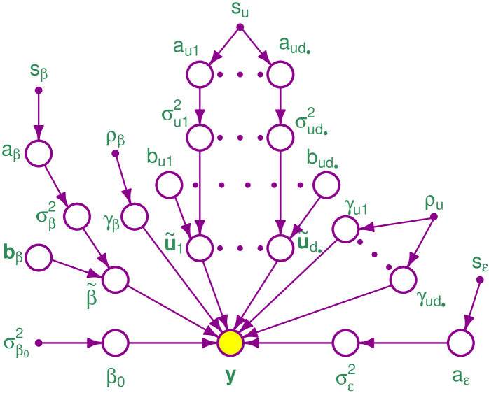
Figure 1: Directed acyclic graph representation of Bayesian model (9). Random variables and vectors are shown as larger open circles, with shading indicating to the observed response data. The small closed circles are user-specified hyperparameters.

2.9 Adjustment for Binary Responses

Now suppose that the $y_{i}$ values are binary rather than continuous. Then an appropriate adjustment to (9) is that where the likelihood is changed to

$${\begin{array}[]{l}y_{i}\big{|}\beta_{0},\boldsymbol{\gamma}_{\mbox{\tiny{$\beta$}}},{\widetilde{\boldsymbol{\beta}}},\gamma_{u1},\ldots,\gamma_{ud_{\bullet}},{\widetilde{\boldsymbol{u}}}_{1},\ldots,{\widetilde{\boldsymbol{u}}}_{d_{\bullet}}\\[4.30554pt] \qquad\qquad\stackrel{{\scriptstyle{\tiny\mbox{ind.}}}}{{\sim}}\mbox{Bernoulli}\Bigg{(}\Phi\Bigg{(}\beta_{0}+\Big{(}\boldsymbol{X}(\boldsymbol{\gamma}_{\mbox{\tiny{$\beta$}}}\odot{\widetilde{\boldsymbol{\beta}}})+{\displaystyle\sum_{j=1}^{d_{\bullet}}}\boldsymbol{Z}_{j}(\gamma_{\mbox{\scriptsize{$u$}\scriptsize{$j$}}}{\widetilde{\boldsymbol{u}}}_{j})\Big{)}_{i}\Bigg{)}\Bigg{)}.\end{array}}$$ (10)

Following Albert & Chib (1993), we introduce auxiliary random variables $c_{1},\ldots,c_{n}$ such that

$$y_{i}=1\quad\mbox{if and only if}\quad c_{i}\geq 0$$ (11)

and impose the following conditional distribution on $\boldsymbol{c}\equiv(c_{1},\ldots,c_{n})$:

$${\begin{array}[]{rcl}&&\boldsymbol{c}|\beta_{0},\boldsymbol{\gamma}_{\mbox{\tiny{$\beta$}}},{\widetilde{\boldsymbol{\beta}}},\gamma_{u1},\ldots,\gamma_{ud_{\bullet}},{\widetilde{\boldsymbol{u}}}_{1},\ldots,{\widetilde{\boldsymbol{u}}}_{d_{\bullet}}\sim\\[4.30554pt] &&\qquad\qquad N\left(\boldsymbol{1}_{n}\beta_{0}+\boldsymbol{X}(\boldsymbol{\gamma}_{\mbox{\tiny{$\beta$}}}\odot{\widetilde{\boldsymbol{\beta}}})+{\displaystyle\sum_{j=1}^{d_{\bullet}}}\boldsymbol{Z}_{j}(\gamma_{\mbox{\scriptsize{$u$}\scriptsize{$j$}}}{\widetilde{\boldsymbol{u}}}_{j}),\boldsymbol{I}_{n}\right).\end{array}}$$ (12)

The prior distributions on $\beta_{0},\boldsymbol{\gamma}_{\mbox{\tiny{$\beta$}}},{\widetilde{\boldsymbol{\beta}}},\gamma_{u1},\ldots,\gamma_{ud_{\bullet}}$ and ${\widetilde{\boldsymbol{u}}}_{1},\ldots,{\widetilde{\boldsymbol{u}}}_{d_{\bullet}}$ are the same as in the Gaussian response case. The error variance variables $\sigma_{\varepsilon}^{2}$ and $a_{\varepsilon}$ are not present for binary responses. Therefore, our binary response model is a modification of (9) for which the $\boldsymbol{y}$ distributional specification is replaced by (11) and (12). Figure 2 shows this modification in graphical terms.

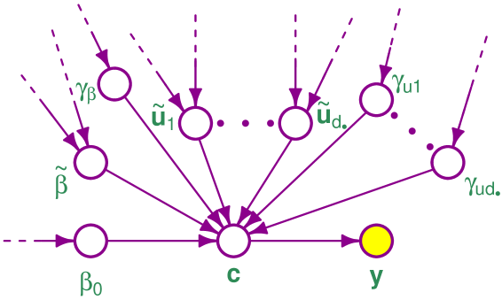
Figure 2: Sub-graph of the directed acyclic graph for the binary response adjustment to (9). This graph is the same as that shown in Figure 1 except for locations near the response variables node. The new graph has the following modifications: (1) the $\sigma_{\varepsilon}^{2}$ and $a_{\varepsilon}$ nodes are absent, (2) a hidden node $\boldsymbol{c}$ corresponding to the Albert-Chib auxiliary variables is added to the position held by $\boldsymbol{y}$ in the Gaussian response graph and the binary response observed data node $\boldsymbol{y}$ is a child of $\boldsymbol{c}$.

3 Practical Fitting and Model Selection

Practical generalized additive model selection based on the models described in Section 2 requires approximation of the posterior distributions of each of the hidden nodes (unshaded circles) in Figures 1 and 2. The problem reduces to approximation conditional marginalization of directed acyclic graphs. The most accurate practical approach is Markov chain Monte Carlo (e.g. Gelfand & Smith, 1990). For the Gaussian response model (9) and its binary response adjustment described in Section 2.9, Section 3.3 provides full algorithmic details for Markov chain Monte Carlo-based approximate conditional marginalization. A faster, but less accurate, alternative is mean field variational Bayes (e.g. Wainwright & Jordan, 2008). To facilitate scalability to very large data sets, we also provide a variational approximate conditional marginalization algorithm in Section 3.4. Both approaches have steps that depend on the data only through particular sufficient statistic quantities. Therefore, there are considerable speed gains from computing and storing these quantities as part of a pre-preprocessing phase.

3.1 Pre-Processing and Storage of Key Matrices

Algorithm 1 is an important part of our overall strategy for fitting our Bayesian generalized additive models in a stable and efficient manner. The first steps involve standardizing the input data and storing the linear transformation parameters to allow conversion of the final results to the original units. Then design matrices denoted by $\boldsymbol{X}$ and $\boldsymbol{Z}$ are computed, with the latter containing all required spline basis functions of the transformed predictor data. Lastly, sufficient statistic matrices such as $\boldsymbol{X}^{T}\boldsymbol{y}$ and $\boldsymbol{Z}^{T}\boldsymbol{Z}$ are computed and stored – ready for use in the upcoming Markov chain Monte Carlo and variational algorithms.

In Algorithm 1 and the upcoming discussion and algorithms we use the identifiers:

$$\textbf{XTy},\ \textbf{XTX},\ \textbf{XTy},\ \textbf{ZTy},\ \textbf{ZTX}\quad\mbox{and}\quad\textbf{ZTZ}$$

for storage of the sufficient statistic quantities $\boldsymbol{X}^{T}\boldsymbol{y}$, $\boldsymbol{X}^{T}\boldsymbol{X}$, $\boldsymbol{X}^{T}\boldsymbol{y}$, $\boldsymbol{Z}^{T}\boldsymbol{y}$, $\boldsymbol{Z}^{T}\boldsymbol{X}$ and $\boldsymbol{Z}^{T}\boldsymbol{Z}$.

• Inputs: $\boldsymbol{y}^{\mbox{\tiny orig}}(n\times 1)$; $\accentset{\circ}{\boldsymbol{x}}^{\mbox{\tiny orig}}_{j}(n\times 1)$, $1\leq j\leq d_{\circ}$; $\accentset{\mbox{\mbox{{$\bullet$}}}}{\boldsymbol{x}}^{\mbox{\tiny orig}}_{j}(n\times 1)$, $1\leq j\leq d_{\bullet}$

• $\mbox{mean}(\boldsymbol{y}^{\mbox{\tiny orig}})\longleftarrow\mbox{sample mean of $\boldsymbol{y}^{\mbox{\tiny orig}}$}\ \ ;\ \ \mbox{st.dev}(\boldsymbol{y}^{\mbox{\tiny orig}})\longleftarrow\mbox{sample standard dev'n of $\boldsymbol{y}^{\mbox{\tiny orig}}$}$

• If $\boldsymbol{y}^{\mbox{\tiny orig}}$ is continuous then $\boldsymbol{y}\longleftarrow\big{\{}\boldsymbol{y}^{\mbox{\tiny orig}}-\mbox{mean}(\boldsymbol{y}^{\mbox{\tiny orig}})\boldsymbol{1}_{n}\big{\}}/\mbox{st.dev}(\boldsymbol{y}^{\mbox{\tiny orig}})$

• If $\boldsymbol{y}^{\mbox{\tiny orig}}$ is binary then $\boldsymbol{y}\longleftarrow\boldsymbol{y}^{\mbox{\tiny orig}}$

• For $j=1,\ldots,d_{\circ}$:

  • $\mbox{mean}(\accentset{\circ}{\boldsymbol{x}}^{\mbox{\tiny orig}}_{j})\longleftarrow\mbox{sample mean of $\accentset{\circ}{\boldsymbol{x}}^{\mbox{\tiny orig}}_{j}$}\ \ ;\ \ \mbox{st.dev.}(\accentset{\circ}{\boldsymbol{x}}^{\mbox{\tiny orig}}_{j})\longleftarrow\mbox{sample standard dev'n of $\accentset{\circ}{\boldsymbol{x}}^{\mbox{\tiny orig}}_{j}$}$

  • $\accentset{\circ}{\boldsymbol{x}}_{j}\longleftarrow\big{\{}\accentset{\circ}{\boldsymbol{x}}^{\mbox{\tiny orig}}_{j}-\mbox{mean}(\accentset{\circ}{\boldsymbol{x}}^{\mbox{\tiny orig}}_{j})\boldsymbol{1}_{n}\big{\}}/\mbox{st.dev.}(\accentset{\circ}{\boldsymbol{x}}^{\mbox{\tiny orig}}_{j})$

• For $j=1,\ldots,d_{\bullet}$:

  • $\mbox{mean}(\accentset{\mbox{\mbox{{$\bullet$}}}}{\boldsymbol{x}}^{\mbox{\tiny orig}}_{j})\longleftarrow\mbox{sample mean of $\accentset{\mbox{\mbox{{$\bullet$}}}}{\boldsymbol{x}}^{\mbox{\tiny orig}}_{j}$}\ \ ;\ \ \mbox{st.dev.}(\accentset{\mbox{\mbox{{$\bullet$}}}}{\boldsymbol{x}}^{\mbox{\tiny orig}}_{j})\longleftarrow\mbox{sample standard dev'n of $\accentset{\mbox{\mbox{{$\bullet$}}}}{\boldsymbol{x}}^{\mbox{\tiny orig}}_{j}$}$

  • $\accentset{\mbox{\mbox{{$\bullet$}}}}{\boldsymbol{x}}_{j}\longleftarrow\big{\{}\accentset{\mbox{\mbox{{$\bullet$}}}}{\boldsymbol{x}}^{\mbox{\tiny orig}}_{j}-\mbox{mean}(\accentset{\mbox{\mbox{{$\bullet$}}}}{\boldsymbol{x}}^{\mbox{\tiny orig}}_{j})\boldsymbol{1}_{n}\big{\}}/\mbox{st.dev.}(\accentset{\mbox{\mbox{{$\bullet$}}}}{\boldsymbol{x}}^{\mbox{\tiny orig}}_{j})$

• $\boldsymbol{X}\longleftarrow\Big{[}\accentset{\circ}{\boldsymbol{x}}_{1}\cdots\accentset{\circ}{\boldsymbol{x}}_{d_{\circ}}\ \accentset{\mbox{\mbox{{$\bullet$}}}}{\boldsymbol{x}}_{1}\cdots\accentset{\mbox{\mbox{{$\bullet$}}}}{\boldsymbol{x}}_{d_{\bullet}}\Big{]}$

• For $j=1,\ldots,d_{\bullet}$:

  • $\boldsymbol{Z}_{j}\longleftarrow\textrm{$n\times K_{j}$ matrix containing the canonical Demmler-Reinsch basis for the predictor}$

  •              data vector $\accentset{\mbox{\mbox{{$\bullet$}}}}{\boldsymbol{x}}_{j}$, using the construction described in Section S.1 of the supplement

• $\boldsymbol{Z}\longleftarrow\big{[}\boldsymbol{Z}_{1}\ \cdots\ \boldsymbol{Z}_{d_{\bullet}}\big{]}$  ;  $\textbf{XTy}\longleftarrow\boldsymbol{X}^{T}\boldsymbol{y}$   ;  $\textbf{XTX}\longleftarrow\boldsymbol{X}^{T}\boldsymbol{X}$  ;   $\textbf{ZTy}\longleftarrow\boldsymbol{Z}^{T}\boldsymbol{y}$
  

• $\textbf{ZTX}\longleftarrow\boldsymbol{Z}^{T}\boldsymbol{X}$  ;  $\textbf{ZTZ}\longleftarrow\boldsymbol{Z}^{T}\boldsymbol{Z}$

• Outputs: $\boldsymbol{y}$, $\boldsymbol{X}$, $\boldsymbol{Z}_{1},\ldots,\boldsymbol{Z}_{d_{\bullet}}$, XTy, XTX, ZTy, ZTX, ZTZ, $\mbox{mean}(\boldsymbol{y}^{\mbox{\tiny orig}})$, $\mbox{st.dev}(\boldsymbol{y}^{\mbox{\tiny orig}})$,
  

• $\qquad\qquad\ \Big{\{}\big{(}\mbox{mean}(\accentset{\circ}{\boldsymbol{x}}^{\mbox{\tiny orig}}_{j}),\mbox{st.dev.}(\accentset{\circ}{\boldsymbol{x}}^{\mbox{\tiny orig}}_{j})\big{)}:1\leq j\leq d_{\circ}\Big{\}}$, $\Big{\{}\big{(}\mbox{mean}(\accentset{\mbox{\mbox{{$\bullet$}}}}{\boldsymbol{x}}^{\mbox{\tiny orig}}_{j}),\mbox{st.dev.}(\accentset{\mbox{\mbox{{$\bullet$}}}}{\boldsymbol{x}}^{\mbox{\tiny orig}}_{j})\big{)}:1\leq j\leq d_{\bullet}\Big{\}}$

Algorithm 1 Pre-processing of original data and creation of key matrices for input into Bayesian generalized additive model algorithms.

3.2 Notation Used in the Fitting Algorithms

For the main fitting algorithms it is useful to have the following definitions in place:

$$K_{j}\equiv\mbox{the number of columns in $\boldsymbol{Z}_{j}$},\quad 1\leq j\leq d_{\bullet}$$,

is the vector with entries and ,

,

,

(13)

Note that, according to the notation in (13),

$$\textbf{ZTX}^{\mbox{\scriptsize{$\langle j\rangle$}}}=\boldsymbol{Z}_{j}^{T}\boldsymbol{X}\quad\mbox{and}\quad\textbf{ZTZ}^{\mbox{\scriptsize{$\langle j,j^{\prime}\rangle$}}}=\boldsymbol{Z}_{j}^{T}\boldsymbol{Z}_{j^{\prime}}.$$

The updates in approximate inference iterative algorithms, presented in Sections 3.3 and 3.4, depend on particular columns and rows of the matrices listed in (13). These will be specified using the following notational convention: $\boldsymbol{e}_{r}$ is a column vector of appropriate length with $r$th entry equal to $1$ and zeroes elsewhere. For example, the $j$th column of XTX is $\textbf{XTX}\boldsymbol{e}_{j}$ where $\boldsymbol{e}_{j}$ is the $(d_{\circ}+d_{\bullet})\times 1$ vector with $j$th entry 1 and $0$ elsewhere. Implementations of the upcoming algorithms normally would not require explicit calculation and storage of $\boldsymbol{e}_{r}$ vectors and, instead, array subsetting code specific to the programming language can be used. However, for algorithm listing use of the $\boldsymbol{e}_{r}$ notation has the advantage of avoiding further subscripting.

To allow the Gaussian and Bernoulli response cases to be handled together we also use the notation $\textbf{yT1}_{\mbox{\scriptsize{adj}}}$, $\textbf{XTy}_{\mbox{\scriptsize{adj}}}$ and $\textbf{ZTy}_{\mbox{\scriptsize{adj}}}$. These are adjustments of yT1, XTy and ZTy in which the $\boldsymbol{y}$ vector is replaced by $\boldsymbol{c}$: the Albert-Chib auxiliary variables vector that arises in the Bernoulli response case. The notation of (13) for extraction of sub-blocks of ZTy also applies to $\textbf{ZTy}_{\mbox{\scriptsize{adj}}}$.

The main algorithms also uses the following functions:

$$\mbox{logit}(x)\equiv\log\left(\frac{x}{1-x}\right),\ \ \mbox{expit}(x)\equiv\mbox{logit}^{-1}(x)=\frac{1}{1+\exp(-x)}\ \ \mbox{and}\ \ \zeta(x)=\log\{2\Phi(x)\}$$

where, as before, $\Phi$ is the $N(0,1)$ cumulative distribution function. It follows that $\zeta^{\prime}(x)=\phi(x)/\Phi(x)$, where $\phi$ is the $N(0,1)$ density function, which arises in Algorithm 3. Stable computation of $\zeta^{\prime}(x)$ when $x$ is a large negative number is not straightforward. Azzalini (2023) and Wand & Ormerod (2012), for example, provide practical solutions to this problem. Lastly, an expression of the form $\zeta^{\prime}(\boldsymbol{v})$, where $\boldsymbol{v}$ is a column vector, is such that function evaluation is element-wise.

3.3 Markov Chain Monte Carlo

For the Bayesian graphical model (9) and the binary response adjustments given in Section 2.9, determination of each of the full conditional distributions for Markov Chain Monte Carlo sampling is fairly straightforward. Virtually all of the full conditional distributions have standard forms such as Bernoulli, Beta, Inverse Gamma and Multivariate Normal distributions. Possible exceptions are the Inverse Gaussian and Truncated Normal distributions, but are such that effective solutions are provided, respectively, by Michael et al. (1976) and Robert (1995). Therefore, Markov Chain Monte Carlo sampling essentially reduces to Gibbs sampling for the models at hand. Algorithm 2 lists the full set of steps needed to draw samples from the posterior distributions of the model parameters. The fact that most of the draws only require the sufficient statistic matrices from Algorithm 1 means that the sampling can be done quite rapidly regardless of sample size.

• Data Inputs: $\boldsymbol{y}\ (n\times 1)$;   $\boldsymbol{X}\ \big{(}n\times(d_{\circ}+d_{\bullet})\big{)}$;   $\boldsymbol{Z}_{j}\ (n\times K_{j})$, $1\leq j\leq d_{\bullet}$.

• Response Type Input: $\textbf{responseType}\in\{\mbox{Gaussian},\mbox{Bernoulli}\}.$

• Sufficient Statistics Inputs: XTy, XTX, ZTy, ZTX, ZTZ.

• Hyperparameter Inputs: $\sigma_{\beta_{0}},s_{\mbox{\tiny{$\beta$}}},s_{\varepsilon},s_{u}>0,\ \ 0\leq\rho_{\mbox{\tiny{$\beta$}}},\rho_{\mbox{\tiny{$u$}}}\leq 1$.

• Chain Length Inputs: $N_{\mbox{\tiny warm}}$ and $N_{\mbox{\tiny kept}}$, both positive integers.
  

• Initialize: $\boldsymbol{\gamma}_{\mbox{\tiny{$\beta$}}}^{[0]}\longleftarrow{\textstyle{\frac{1}{2}}}\boldsymbol{1}_{d_{\circ}+d_{\bullet}}$; $\gamma_{\mbox{\scriptsize{$u$}\scriptsize{$j$}}}^{[0]}\longleftarrow{\textstyle{\frac{1}{2}}}$, $1\leq j\leq d_{\bullet}$;  ${\widetilde{\boldsymbol{\beta}}}^{[0]}\longleftarrow\boldsymbol{0}_{d_{\circ}+d_{\bullet}}$
  

• $\qquad\qquad{\widetilde{\boldsymbol{u}}}_{j}^{[0]}\longleftarrow\boldsymbol{0}_{K_{j}}$, $1\leq j\leq d_{\bullet}$;  $a_{\varepsilon}^{[0]}\longleftarrow 1$;  $(\sigma_{\varepsilon}^{2})^{[0]}\longleftarrow 1$;  $(\sigma_{\mbox{\tiny{$\beta$}}}^{2})^{[0]}\longleftarrow 1$ ;  $a_{\beta}^{[0]}\longleftarrow 1$
  

• $\qquad\qquad\boldsymbol{b}_{\mbox{\tiny{$\beta$}}}^{[0]}\longleftarrow\boldsymbol{1}_{d_{\circ}+d_{\bullet}}$  ;  $b_{\mbox{\scriptsize{$u$}\scriptsize{$j$}}}^{[0]}\longleftarrow 1$, $1\leq j\leq d_{\bullet}$
  

• $\qquad\qquad a_{uj}^{[0]}\longleftarrow 1$, $1\leq j\leq d_{\bullet}$;  $(\sigma_{uj}^{2})^{[0]}\longleftarrow 1$, $1\leq j\leq d_{\bullet}$.
  

• $\textbf{yT1}_{\mbox{\scriptsize{adj}}}\longleftarrow 0$  ;  $\textbf{XTy}_{\mbox{\scriptsize{adj}}}\longleftarrow\textbf{XTy}$   ;  $\textbf{ZTy}_{\mbox{\scriptsize{adj}}}\longleftarrow\textbf{ZTy}$
  

• For $j=1,\ldots,d_{\bullet}$:$\quad\boldsymbol{w}_{\mbox{\tiny$\boldsymbol{Z}$}j}\longleftarrow\mbox{diagonal}\big{(}\textbf{ZTZ}^{\mbox{\scriptsize{$\langle j,j\rangle$}}}\big{)}$

• For $g=1,\ldots,N_{\mbox{\tiny warm}}+N_{\mbox{\tiny kept}}$:
  

  • $\omega_{1}\longleftarrow\textbf{yT1}_{\mbox{\scriptsize{adj}}}$
    

  • $\omega_{2}\longleftarrow\big{\{}n\big{/}(\sigma_{\varepsilon}^{2})^{[g-1]}\big{\}}+(1/\sigma_{\beta_{0}}^{2})$    ;   $\beta_{0}^{[g]}\sim\displaystyle{N\left(\frac{\omega_{1}}{(\sigma_{\varepsilon}^{2})^{[g-1]}\omega_{2}},\frac{1}{\omega_{2}}\right)}$
    

  • $\boldsymbol{\Omega}\longleftarrow\left(\boldsymbol{\gamma}_{\mbox{\tiny{$\beta$}}}^{[g-1]}\boldsymbol{\gamma}_{\mbox{\tiny{$\beta$}}}^{[g-1]T}\right)\odot(\textbf{XTX})\Big{/}(\sigma_{\varepsilon}^{2})^{[g-1]}+\mbox{diag}\left(\boldsymbol{b}_{\mbox{\tiny{$\beta$}}}^{[g-1]}\right)\Big{/}(\sigma_{\mbox{\tiny{$\beta$}}}^{2})^{[g-1]}$
    

  • $\boldsymbol{\omega}_{3}\longleftarrow\textbf{XTy}_{\mbox{\scriptsize{adj}}}-{\displaystyle\sum_{j=1}^{d_{\bullet}}}\textbf{ZTX}^{\mbox{\scriptsize{$\langle j\rangle$}}T}\big{(}\gamma_{\mbox{\scriptsize{$u$}\scriptsize{$j$}}}^{[g-1]}{\widetilde{\boldsymbol{u}}}_{j}^{[g-1]}\big{)}$
    

  • Decompose $\boldsymbol{\Omega}=\boldsymbol{U}_{\mbox{\tiny{$\boldsymbol{\Omega}$}}}\mbox{diag}(\boldsymbol{d}_{\mbox{\tiny{$\boldsymbol{\Omega}$}}})\boldsymbol{U}_{\mbox{\tiny{$\boldsymbol{\Omega}$}}}^{T}$ where $\boldsymbol{U}_{\mbox{\tiny{$\boldsymbol{\Omega}$}}}\boldsymbol{U}_{\mbox{\tiny{$\boldsymbol{\Omega}$}}}^{T}=\boldsymbol{I}$
    

  • $\boldsymbol{z}\sim N(\boldsymbol{0},\boldsymbol{I})\ \big{(}(d_{\circ}+d_{\bullet})\times 1\big{)}$   ;   ${\widetilde{\boldsymbol{\beta}}}^{[g]}\longleftarrow\boldsymbol{U}_{\mbox{\tiny{$\boldsymbol{\Omega}$}}}\displaystyle{\left(\frac{\boldsymbol{U}_{\mbox{\tiny{$\boldsymbol{\Omega}$}}}^{T}\boldsymbol{z}}{\sqrt{\boldsymbol{d}_{\mbox{\tiny{$\boldsymbol{\Omega}$}}}}}+\frac{\boldsymbol{U}_{\mbox{\tiny{$\boldsymbol{\Omega}$}}}^{T}\left(\boldsymbol{\gamma}_{\mbox{\tiny{$\beta$}}}^{[g-1]}\odot\boldsymbol{\omega}_{3}\right)}{\boldsymbol{d}_{\mbox{\tiny{$\boldsymbol{\Omega}$}}}(\sigma_{\varepsilon}^{2})^{[g-1]}}\right)}$
    

  • $\big{(}\boldsymbol{b}_{\mbox{\tiny{$\beta$}}}^{[g]})_{j}\sim\mbox{Inverse-Gaussian}\Big{(}\sigma_{\mbox{\tiny{$\beta$}}}^{[g-1]}\Big{/}\Big{|}\big{(}{\widetilde{\boldsymbol{\beta}}}^{[g]}\big{)}_{j}\Big{|}\Big{)},\quad 1\leq j\leq d_{\circ}+d_{\bullet}$
    

  • $(\sigma_{\mbox{\tiny{$\beta$}}}^{2})^{[g]}\sim\mbox{Inverse-Gamma}\displaystyle{\left({\textstyle{\frac{1}{2}}}(d_{\circ}+d_{\bullet}+1),1/a_{\beta}^{[g-1]}+{\textstyle{\frac{1}{2}}}{\widetilde{\boldsymbol{\beta}}}^{[g]T}\mbox{diag}\left(\boldsymbol{b}_{\mbox{\tiny{$\beta$}}}^{[g]}\right){\widetilde{\boldsymbol{\beta}}}^{[g]}\right)}$

  • $a_{\mbox{\tiny{$\beta$}}}^{[g]}\sim\mbox{Inverse-Gamma}\displaystyle{\left(1,\big{\{}1\big{/}(\sigma_{\mbox{\tiny{$\beta$}}}^{2})^{[g]}\big{\}}+(1/s_{\mbox{\tiny{$\beta$}}}^{2})\right)}$   ;  $\boldsymbol{\beta}^{\mbox{\tiny{curr}}}\longleftarrow\boldsymbol{\gamma}_{\mbox{\tiny{$\beta$}}}^{[g-1]}\odot{\widetilde{\boldsymbol{\beta}}}^{[g]}$

  • For $j=1,\ldots,d_{\bullet}$: $\quad\boldsymbol{u}_{j}^{\mbox{\tiny{curr}}}\longleftarrow\gamma_{\mbox{\scriptsize{$u$}\scriptsize{$j$}}}^{[g-1]}{\widetilde{\boldsymbol{u}}}_{j}^{[g-1]}$

  • For $j=1,\ldots,d_{\circ}+d_{\bullet}$:
    

    • $\omega_{4}\longleftarrow\boldsymbol{e}_{j}^{T}\textbf{XTy}_{\mbox{\scriptsize{adj}}}-\big{(}\textbf{XTX}\boldsymbol{e}_{j}\big{)}_{-j}^{T}\big{(}\boldsymbol{\beta}^{\mbox{\tiny{curr}}})_{-j}-\displaystyle{\sum_{j^{\prime}=1}^{d_{\bullet}}}\Big{(}\textbf{ZTX}^{\mbox{\scriptsize{$\langle j^{\prime}\rangle$}}}\boldsymbol{e}_{j}\Big{)}^{T}\boldsymbol{u}_{j^{\prime}}^{\mbox{\tiny{curr}}}$

    • $\omega_{5}\longleftarrow\mbox{logit}(\rho_{\mbox{\tiny{$\beta$}}})-{\textstyle{\frac{1}{2}}}\Big{\{}\big{(}{\widetilde{\beta}}_{j}^{[g]}\big{)}^{2}\boldsymbol{e}_{j}^{T}\textbf{XTX}\boldsymbol{e}_{j}-2{\widetilde{\beta}}_{j}^{[g]}\omega_{4}\Big{\}}\Big{/}(\sigma_{\varepsilon}^{2})^{[g-1]}$

    • $\big{(}\boldsymbol{\gamma}_{\mbox{\tiny{$\beta$}}}^{[g]})_{j}\sim\mbox{Bernoulli}\big{(}\mbox{expit}(\omega_{5})\big{)}$

  • continued on a subsequent page $\ldots$
    

Algorithm 2 Markov chain Monte Carlo generation of samples from the posterior distributions of the parameters in (9).

• • $\boldsymbol{\beta}^{\mbox{\tiny{curr}}}\longleftarrow\boldsymbol{\gamma}_{\mbox{\tiny{$\beta$}}}^{[g]}\odot{\widetilde{\boldsymbol{\beta}}}^{[g]}$   ;   For $j=1,\ldots,d_{\bullet}$: $\quad{\widetilde{\boldsymbol{u}}}_{j}^{\mbox{\tiny{curr}}}\longleftarrow{\widetilde{\boldsymbol{u}}}_{j}^{[g-1]}$

  • For $j=1,\ldots,d_{\bullet}$:
    

    • $\boldsymbol{\omega}_{6}\longleftarrow\textbf{ZTy}^{\mbox{\scriptsize{$\langle j\rangle$}}}_{\mbox{\scriptsize{adj}}}-\textbf{ZTX}^{\mbox{\scriptsize{$\langle j\rangle$}}}\boldsymbol{\beta}^{\mbox{\tiny{curr}}}-{\displaystyle\sum_{j^{\prime}\neq j}^{d_{\bullet}}}\textbf{ZTZ}^{\mbox{\scriptsize{$\langle j,j^{\prime}\rangle$}}}\big{(}\gamma_{u\,j^{\prime}}^{[g-1]}{\widetilde{\boldsymbol{u}}}_{j^{\prime}}^{\mbox{\tiny{curr}}}\big{)}$

    • $\boldsymbol{\omega}_{7}\longleftarrow\Big{\{}\gamma_{\mbox{\scriptsize{$u$}\scriptsize{$j$}}}^{[g-1]}\boldsymbol{w}_{\mbox{\tiny$\boldsymbol{Z}$}j}\Big{/}(\sigma_{\varepsilon}^{2})^{[g-1]}\Big{\}}+\Big{\{}b_{\mbox{\scriptsize{$u$}\scriptsize{$j$}}}^{[g-1]}\boldsymbol{1}_{K_{j}}\Big{/}(\sigma_{uj}^{2})^{[g-1]}\Big{\}}$

    • $\boldsymbol{z}\sim N(\boldsymbol{0},\boldsymbol{I}_{K_{j}})$   ;   ${\widetilde{\boldsymbol{u}}}_{j}^{\mbox{\tiny{curr}}}\longleftarrow\big{(}\boldsymbol{z}\big{/}\sqrt{\boldsymbol{\omega}_{7}}\big{)}+\big{[}\gamma_{\mbox{\scriptsize{$u$}\scriptsize{$j$}}}^{[g-1]}\boldsymbol{\omega}_{6}\big{/}\big{\{}\boldsymbol{\omega}_{7}(\sigma_{\varepsilon}^{2})^{[g-1]}\big{\}}\big{]}$

  • For $j=1,\ldots,d_{\bullet}$: $\quad{\widetilde{\boldsymbol{u}}}_{j}^{[g]}\longleftarrow{\widetilde{\boldsymbol{u}}}_{j}^{\mbox{\tiny{curr}}}$

  • For $j=1,\ldots,d_{\bullet}$:

    • $b_{\mbox{\scriptsize{$u$}\scriptsize{$j$}}}^{[g]}\sim\mbox{Inverse-Gaussian}\left(\sigma_{uj}^{[g-1]}\Big{/}\|{\widetilde{\boldsymbol{u}}}_{j}^{[g]}\|,1\right)$

    • $(\sigma^{2}_{uj})^{[g]}\sim\mbox{Inverse-Gamma}\left({\textstyle{\frac{1}{2}}}(K_{j}+1),\big{\{}1\big{/}a_{uj}^{[g-1]}\big{\}}+{\textstyle{\frac{1}{2}}}\|{\widetilde{\boldsymbol{u}}}_{j}^{[g]}\|^{2}b_{\mbox{\scriptsize{$u$}\scriptsize{$j$}}}^{[g]}\right)$

    • $a_{uj}^{[g]}\sim\mbox{Inverse-Gamma}\displaystyle{\left(1,\{1\big{/}(\sigma^{2}_{uj})^{[g]}\}+(1/s_{u}^{2})\right)}$

  • For $j=1,\ldots,d_{\bullet}$: $\quad\gamma_{\mbox{\tiny{$u$}}\mbox{\scriptsize{$j$}}}^{\mbox{\tiny{curr}}}\longleftarrow\gamma_{\mbox{\scriptsize{$u$}\scriptsize{$j$}}}^{[g-1]}$
    

  • For $j=1,\ldots,d_{\bullet}$:
    

    • $\boldsymbol{\omega}_{8}\longleftarrow\textbf{ZTy}^{\mbox{\scriptsize{$\langle j\rangle$}}}_{\mbox{\scriptsize{adj}}}-\textbf{ZTX}^{\mbox{\scriptsize{$\langle j\rangle$}}}\boldsymbol{\beta}^{\mbox{\tiny{curr}}}-\displaystyle{\sum_{j^{\prime}\neq j}^{d_{\bullet}}}\textbf{ZTZ}^{\mbox{\scriptsize{$\langle j,j^{\prime}\rangle$}}}\big{(}\gamma_{\mbox{\tiny{$u$}}\mbox{\scriptsize{$j^{\prime}$}}}^{\mbox{\tiny{curr}}}\,{\widetilde{\boldsymbol{u}}}_{j^{\prime}}^{[g]}\big{)}$
      

    • $\omega_{9}\longleftarrow\mbox{logit}\left(\rho_{\mbox{\tiny{$u$}}}\right)-{\textstyle{\frac{1}{2}}}\Big{\{}\boldsymbol{w}_{\mbox{\tiny$\boldsymbol{Z}$}j}^{T}\big{(}{\widetilde{\boldsymbol{u}}}_{j}^{[g]}\odot{\widetilde{\boldsymbol{u}}}_{j}^{[g]}\big{)}-2\big{(}{\widetilde{\boldsymbol{u}}}_{j}^{[g]}\big{)}^{T}\boldsymbol{\omega}_{8}\Big{\}}\Big{/}(\sigma_{\varepsilon}^{2})^{[g-1]}$

    • $\gamma_{\mbox{\tiny{$u$}}\mbox{\scriptsize{$j$}}}^{\mbox{\tiny{curr}}}\sim\mbox{Bernoulli}\big{(}\mbox{expit}(\omega_{9})\big{)}$

  • For $j=1,\ldots,d_{\bullet}$: $\quad\gamma_{\mbox{\scriptsize{$u$}\scriptsize{$j$}}}^{[g]}\longleftarrow\gamma_{\mbox{\tiny{$u$}}\mbox{\scriptsize{$j$}}}^{\mbox{\tiny{curr}}}$
    

  • $\boldsymbol{\omega}_{10}\longleftarrow\boldsymbol{1}_{n}\beta_{0}^{[g]}+\boldsymbol{X}\left(\boldsymbol{\gamma}_{\mbox{\tiny{$\beta$}}}^{[g]}\odot{\widetilde{\boldsymbol{\beta}}}^{[g]}\right)+\displaystyle{\sum_{j=1}^{d_{\bullet}}}\boldsymbol{Z}_{j}\left(\gamma_{\mbox{\scriptsize{$u$}\scriptsize{$j$}}}^{[g]}\,{\widetilde{\boldsymbol{u}}}_{j}^{[g]}\right)$

  • If responseType  is Gaussian then

    • $(\sigma_{\varepsilon}^{2})^{[g]}\sim\mbox{Inverse-Gamma}\left({\textstyle{\frac{1}{2}}}(n+1),\big{(}1\big{/}a_{\varepsilon}^{[g-1]}\big{)}+{\textstyle{\frac{1}{2}}}\|\boldsymbol{y}-\boldsymbol{\omega}_{10}\|^{2}\right)$

    • $a_{\varepsilon}^{[g]}\sim\mbox{Inverse-Gamma}\displaystyle{\left(1,\big{\{}1\big{/}(\sigma_{\varepsilon}^{2})^{[g]}\big{\}}+(1/s_{\varepsilon}^{2})\right)}$

  • If responseType  is Bernoulli then

    • $(\sigma_{\varepsilon}^{2})^{[g]}\longleftarrow 1$

    • For $i=1,\ldots,n$:

      • $\omega_{11}\sim\mbox{Truncated-Normal}_{+}\big{(}(2y_{i}-1)(\boldsymbol{\omega}_{10})_{i},1\big{)}$  ;  $c_{i}\longleftarrow(2y_{i}-1)\omega_{11}$

    • $\textbf{yT1}_{\mbox{\scriptsize{adj}}}\longleftarrow\boldsymbol{1}^{T}\boldsymbol{c}$  ;   $\textbf{XTy}_{\mbox{\scriptsize{adj}}}\longleftarrow\boldsymbol{X}^{T}\boldsymbol{c}$   ;   $\textbf{ZTy}_{\mbox{\scriptsize{adj}}}\longleftarrow\boldsymbol{Z}^{T}\boldsymbol{c}$

• Outputs: All chains after omission of the first $N_{\mbox{\tiny warm}}$ values.

Algorithm 2 continued. This is a continuation of the description of this algorithm that commences on a preceding page.

3.4 Mean Field Variational Bayes

Mean field variational Bayes approximate fitting and inference for (9) involves approximation of the joint posterior density function of the model parameters by a product density form such as

$${\begin{array}[]{rcl}&&\mathfrak{p}\big{(}\beta_{0},\boldsymbol{\gamma}_{\mbox{\tiny{$\beta$}}},{\widetilde{\boldsymbol{\beta}}},\boldsymbol{\gamma}_{\mbox{\tiny{$u$}}},{\widetilde{\boldsymbol{u}}},\boldsymbol{b}_{\mbox{\tiny{$\beta$}}},\sigma^{2}_{\mbox{\tiny{$\beta$}}},a_{\mbox{\tiny{$\beta$}}},\boldsymbol{b}_{\mbox{\tiny{$u$}}},\boldsymbol{\sigma}_{\mbox{\tiny{$u$}}}^{2},\boldsymbol{a}_{\mbox{\tiny{$u$}}},\sigma_{\varepsilon}^{2},a_{\varepsilon}|\boldsymbol{y}\big{)}\\[4.30554pt] &&\quad\qquad\approx\mathfrak{q}(\beta_{0})\mathfrak{q}(\boldsymbol{\gamma}_{\mbox{\tiny{$\beta$}}})\mathfrak{q}({\widetilde{\boldsymbol{\beta}}})\mathfrak{q}(\boldsymbol{\gamma}_{\mbox{\tiny{$u$}}})\mathfrak{q}({\widetilde{\boldsymbol{u}}})\mathfrak{q}(\boldsymbol{b}_{\mbox{\tiny{$\beta$}}})\mathfrak{q}(\sigma_{\beta}^{2})\mathfrak{q}(a_{\mbox{\tiny{$\beta$}}})\mathfrak{q}(\boldsymbol{b}_{\mbox{\tiny{$u$}}})\mathfrak{q}(\boldsymbol{\sigma}_{\mbox{\tiny{$u$}}}^{2})\mathfrak{q}(\boldsymbol{a}_{\mbox{\tiny{$u$}}})\mathfrak{q}(\sigma_{\varepsilon}^{2})\mathfrak{q}(a_{\varepsilon})\end{array}}$$ (14)

where, for example, ${\widetilde{\boldsymbol{u}}}\equiv({\widetilde{\boldsymbol{u}}}_{1},\ldots,{\widetilde{\boldsymbol{u}}}_{d_{\bullet}})$ and $\boldsymbol{b}_{\mbox{\tiny{$\beta$}}}\equiv\big{(}b_{\mbox{\tiny{$\beta$}\scriptsize{$1$}}},\ldots,b_{\mbox{\tiny{$\beta$}\scriptsize{$(d_{\circ}+d_{\bullet})$}}}\big{)}$. There are numerous options for the stringency of the product restriction and the choice involves trade-offs concerning tractability, accuracy and speed. For example, one could contemplate replacing $\mathfrak{q}(\beta_{0})\mathfrak{q}({\widetilde{\boldsymbol{\beta}}})\mathfrak{q}({\widetilde{\boldsymbol{u}}})$ in (14) by $\mathfrak{q}(\beta_{0},{\widetilde{\boldsymbol{\beta}}},{\widetilde{\boldsymbol{u}}})$ and improve the accuracy of approximation. However, the more stringent approximation is less tractable. In addition to the product restriction (14) we also impose the product density restrictions:

$$\mathfrak{q}(\gamma_{\mbox{\tiny{$\beta$}}})=\prod_{j=1}^{d_{\circ}+d_{\bullet}}\mathfrak{q}(\gamma_{\mbox{\tiny{$\beta$}\scriptsize{$j$}}}),\quad\mathfrak{q}({\widetilde{\boldsymbol{u}}})=\prod_{j=1}^{d_{\bullet}}\mathfrak{q}({\widetilde{\boldsymbol{u}}}_{j})\quad\mbox{and}\quad\mathfrak{q}(\boldsymbol{\gamma}_{\mbox{\tiny{$u$}}})=\prod_{j=1}^{d_{\bullet}}\mathfrak{q}(\gamma_{\mbox{\scriptsize{$u$}\scriptsize{$j$}}}).$$ (15)

With the product density restrictions in place, we obtain the optimal $\mathfrak{q}$-densities by minimising the Kullback-Leibler divergence of the left-hand side of (14) from the right-hand side. The optimal $\mathfrak{q}$-density forms can be expressed in terms of the full conditional density functions as given by equation (6) of Ormerod & Wand (2010). The optimal $\mathfrak{q}$-density parameters can then be solved via a coordinate ascent algorithm. Since each of the full conditionals in the models at hand have standard forms, the optimal $\mathfrak{q}$-density functions are relatively simple and the coordinate ascent updates have closed forms.

The Bayesian graphical model for wavelet regression described in Section 3 of Wand & Ormerod (2011) is similar in nature to the generalized additive selection model (9). Hence, the relevant details on the requisite mean field variational Bayes calculations for (9) can be gleaned from the $\mathfrak{q}$-density derivations given in Appendix D of Wand & Ormerod (2011).

Some examples of the resulting optimal $\mathfrak{q}$-density forms are:

$$\begin{array}[]{rcl}&&\mathfrak{q}({\widetilde{\boldsymbol{\beta}}})\ \mbox{has a}\ N\big{(}\boldsymbol{\mu}_{\mathfrak{q}({\widetilde{\boldsymbol{\beta}}})},\boldsymbol{\Sigma}_{\mathfrak{q}({\widetilde{\boldsymbol{\beta}}})}\big{)}\ \mbox{density function, and }\\[0.0pt] &&\mathfrak{q}(\sigma^{2}_{\mbox{\tiny{$\varepsilon$}}})\ \mbox{has an}\ \mbox{Inverse-Gamma}\big{(}\kappa_{\mathfrak{q}(\sigma^{2}_{\mbox{\tiny{$\varepsilon$}}})},\lambda_{\mathfrak{q}(\sigma^{2}_{\mbox{\tiny{$\varepsilon$}}})}\big{)}\ \mbox{density function.}\end{array}$$ (16)

The optimal Inverse Gamma shape parameter $\kappa_{\mathfrak{q}(\sigma^{2}_{\mbox{\tiny{$\varepsilon$}}})}$ has explicit solution ${\textstyle{\frac{1}{2}}}(n+1)$. However, the equations for the optimal values of $\boldsymbol{\mu}_{\mathfrak{q}({\widetilde{\boldsymbol{\beta}}})}$, $\boldsymbol{\Sigma}_{\mathfrak{q}({\widetilde{\boldsymbol{\beta}}})}$ and $\lambda_{\mathfrak{q}(\sigma^{2}_{\mbox{\tiny{$\varepsilon$}}})}$ are interdependent and iteration is required to obtain their optimal values. Algorithm 3 lists the full set of steps required to obtain all $\mathfrak{q}$-density parameters, with notation similar to that used in (16) for the other $\mathfrak{q}$-density parameters.

A final aspect of Algorithm 3 is determination of good stopping criteria for the coordinate ascent scheme. As is common in the mean field variational Bayes literature we monitor relative increases in the approximate marginal log-likelihood, also known as the evidence lower bound, which we denote by $\log\underline{p}(\boldsymbol{y};\mathfrak{q})$. Section S.2 of the supplement contains an explicit expression for the approximate marginal log-likelihood for the Section 2 models under product restrictions (14)–(15).

• Data Inputs: $\boldsymbol{y}\ (n\times 1)$;   $\boldsymbol{X}\ \big{(}n\times(d_{\circ}+d_{\bullet})\big{)}$;   $\boldsymbol{Z}_{j}\ (n\times K_{j})$, $1\leq j\leq d_{\bullet}$.

• Response Type Input: $\textbf{responseType}\in\{\mbox{Gaussian},\mbox{Bernoulli}\}$.

• Sufficient Statistics Inputs: XTy, XTX, ZTy, ZTX, ZTZ

• Hyperparameter Inputs: $\sigma_{\beta_{0}},s_{\mbox{\tiny{$\beta$}}},s_{\varepsilon},s_{u}>0,\ \ 0\leq\rho_{\mbox{\tiny{$\beta$}}},\rho_{\mbox{\tiny{$u$}}}\leq 1$.

• Convergence Criterion Input: $\varepsilon_{\tiny\mbox{toler.}}:\ \mbox{a small positive number such as}\ 10^{-8}$.

• Initialize: $\boldsymbol{\mu}_{\mathfrak{q}(\gamma_{\mbox{\tiny{$\beta$}}})}\longleftarrow{\textstyle{\frac{1}{2}}}\boldsymbol{1}_{d_{\circ}+d_{\bullet}}$  ; $\boldsymbol{\mu}_{\mathfrak{q}({\widetilde{\boldsymbol{\beta}}})}\longleftarrow\boldsymbol{0}_{d_{\circ}+d_{\bullet}}$  ; $\mu_{\mathfrak{q}(1/a_{\varepsilon})}\longleftarrow 1$,  ; $\mu_{\mathfrak{q}(1/\sigma_{\varepsilon}^{2})}\longleftarrow 1$
  

• $\qquad\qquad\ \mu_{\mathfrak{q}(1/a_{\beta})}\longleftarrow 1$ ; $\mu_{\mathfrak{q}(1/\sigma_{\mbox{\tiny{$\beta$}}}^{2})}\longleftarrow 1$ ; $\kappa_{\mathfrak{q}(\sigma_{\mbox{\tiny{$\beta$}}}^{2})}\longleftarrow{\textstyle{\frac{1}{2}}}(d_{\circ}+d_{\bullet}+1)$ ; $\kappa_{\mathfrak{q}(a_{\mbox{\tiny{$\beta$}}})}\longleftarrow 1$
  

• $\qquad\qquad\ \kappa_{\mathfrak{q}(\sigma_{\varepsilon}^{2})}\longleftarrow{\textstyle{\frac{1}{2}}}(n+1)\ ;\ \kappa_{\mathfrak{q}(a_{\varepsilon})}\longleftarrow 1$ ; $\boldsymbol{\mu}_{\mathfrak{q}(\boldsymbol{b}_{\mbox{\tiny{$\beta$}}})}\longleftarrow\boldsymbol{1}_{d_{\circ}+d_{\bullet}}$
  

• $\qquad\qquad\ \textbf{yT1}_{\mbox{\scriptsize{adj}}}\longleftarrow 0$  ;  $\textbf{XTy}_{\mbox{\scriptsize{adj}}}\longleftarrow\textbf{XTy}$  ;  $\textbf{ZTy}_{\mbox{\scriptsize{adj}}}\longleftarrow\textbf{ZTy}$
  

•               For $j=1,\ldots,d_{\bullet}$:
  

  • $\qquad\qquad\ \boldsymbol{\mu}_{\mathfrak{q}({\widetilde{\boldsymbol{u}}}_{j})}\longleftarrow\boldsymbol{0}_{K_{j}}$ ; $\boldsymbol{\sigma}^{2}_{\mathfrak{q}({\widetilde{\boldsymbol{u}}}_{j})}\longleftarrow\boldsymbol{1}_{K_{j}}$ ;  $\mu_{\mathfrak{q}(\gamma_{\mbox{\scriptsize{$u$}\scriptsize{$j$}}})}\longleftarrow{\textstyle{\frac{1}{2}}}$
    

  • $\qquad\qquad\ \mu_{\mathfrak{q}(1/a_{uj})}\longleftarrow 1$ ; $\mu_{\mathfrak{q}(1/\sigma_{uj}^{2})}\longleftarrow 1$ ; $\mu_{\mathfrak{q}(b_{\mbox{\scriptsize{$u$}\scriptsize{$j$}}})}\longleftarrow 1$
    

  • $\qquad\qquad\ \kappa_{\mathfrak{q}(\sigma_{uj}^{2})}\longleftarrow{\textstyle{\frac{1}{2}}}(K_{j}+1)$ ; $\kappa_{\mathfrak{q}(a_{uj})}\longleftarrow 1$ ; $\boldsymbol{w}_{\mbox{\tiny$\boldsymbol{Z}$}j}\longleftarrow\mbox{diagonal}\big{(}\textbf{ZTZ}^{\mbox{\scriptsize{$\langle j,j\rangle$}}}\big{)}$

• Cycle:
  

  • $\omega_{12}\longleftarrow\textbf{yT1}_{\mbox{\scriptsize{adj}}}$
    

  • $\sigma^{2}_{\mathfrak{q}(\beta_{0})}\longleftarrow 1\big{/}\{n\mu_{\mathfrak{q}(1/\sigma_{\varepsilon}^{2})}+(1/\sigma_{\beta_{0}}^{2})\}$   ;   $\mu_{\mathfrak{q}(\beta_{0})}\longleftarrow\sigma^{2}_{\mathfrak{q}(\beta_{0})}\mu_{\mathfrak{q}(1/\sigma_{\varepsilon}^{2})}\omega_{12}$

  • $\boldsymbol{\Omega}_{\mathfrak{q}(\gamma_{\mbox{\tiny{$\beta$}}})}\longleftarrow\mbox{diag}\big{\{}\boldsymbol{\mu}_{\mathfrak{q}(\gamma_{\mbox{\tiny{$\beta$}}})}\odot(\boldsymbol{1}-\boldsymbol{\mu}_{\mathfrak{q}(\gamma_{\mbox{\tiny{$\beta$}}})})\big{\}}+\boldsymbol{\mu}_{\mathfrak{q}(\gamma_{\mbox{\tiny{$\beta$}}})}\boldsymbol{\mu}_{\mathfrak{q}(\gamma_{\mbox{\tiny{$\beta$}}})}^{T}$

  • $\boldsymbol{\Sigma}_{\mathfrak{q}({\widetilde{\boldsymbol{\beta}}})}\longleftarrow\left\{\mu_{\mathfrak{q}(1/\sigma_{\varepsilon}^{2})}\boldsymbol{\Omega}_{\mathfrak{q}(\gamma_{\mbox{\tiny{$\beta$}}})}\odot(\boldsymbol{X}^{T}\boldsymbol{X})+\mu_{\mathfrak{q}(1/\sigma_{\mbox{\tiny{$\beta$}}}^{2})}\mbox{diag}(\boldsymbol{\mu}_{\mathfrak{q}(\boldsymbol{b}_{\mbox{\tiny{$\beta$}}})})\right\}^{-1}$

  • $\boldsymbol{\omega}_{13}\longleftarrow\textbf{XTy}_{\mbox{\scriptsize{adj}}}-{\displaystyle\sum_{j=1}^{d_{\bullet}}}\textbf{ZTX}^{\mbox{\scriptsize{$\langle j\rangle$}}T}\big{(}\mu_{\mathfrak{q}(\gamma_{\mbox{\scriptsize{$u$}\scriptsize{$j$}}})}\,\boldsymbol{\mu}_{\mathfrak{q}({\widetilde{\boldsymbol{u}}}_{j})}\big{)}$
    

  • $\boldsymbol{\mu}_{\mathfrak{q}({\widetilde{\boldsymbol{\beta}}})}\longleftarrow\mu_{\mathfrak{q}(1/\sigma_{\varepsilon}^{2})}\boldsymbol{\Sigma}_{\mathfrak{q}({\widetilde{\boldsymbol{\beta}}})}\big{(}\boldsymbol{\mu}_{\mathfrak{q}(\gamma_{\mbox{\tiny{$\beta$}}})}\odot\boldsymbol{\omega}_{13}\big{)}$

  • $\boldsymbol{\omega}_{14}\longleftarrow\boldsymbol{\mu}_{\mathfrak{q}({\widetilde{\boldsymbol{\beta}}})}\odot\boldsymbol{\mu}_{\mathfrak{q}({\widetilde{\boldsymbol{\beta}}})}+\mbox{diagonal}\big{(}\boldsymbol{\Sigma}_{\mathfrak{q}({\widetilde{\boldsymbol{\beta}}})}\big{)}$   ;   $\boldsymbol{\mu}_{\mathfrak{q}(\boldsymbol{b}_{\mbox{\tiny{$\beta$}}})}\longleftarrow\Big{(}\mu_{\mathfrak{q}(1/\sigma_{\beta}^{2})}\boldsymbol{\omega}_{14}\Big{)}^{-1/2}$

  • $\lambda_{\mathfrak{q}(\sigma_{\mbox{\tiny{$\beta$}}}^{2})}\longleftarrow\mu_{\mathfrak{q}(1/a_{\beta})}+{\textstyle{\frac{1}{2}}}\boldsymbol{\mu}_{\mathfrak{q}(\boldsymbol{b}_{\mbox{\tiny{$\beta$}}})}^{T}\boldsymbol{\omega}_{14}$   ;   $\mu_{\mathfrak{q}(1/\sigma_{\mbox{\tiny{$\beta$}}}^{2})}\longleftarrow\kappa_{\mathfrak{q}(\sigma_{\mbox{\tiny{$\beta$}}}^{2})}/\lambda_{\mathfrak{q}(\sigma_{\mbox{\tiny{$\beta$}}}^{2})}$

  • $\lambda_{\mathfrak{q}(a_{\mbox{\tiny{$\beta$}}})}\longleftarrow\mu_{\mathfrak{q}(1/\sigma_{\mbox{\tiny{$\beta$}}}^{2})}+s_{\mbox{\tiny{$\beta$}}}^{-2}$   ;   $\mu_{\mathfrak{q}(1/a_{\mbox{\tiny{$\beta$}}})}\longleftarrow\kappa_{\mathfrak{q}(a_{\mbox{\tiny{$\beta$}}})}\big{/}\lambda_{\mathfrak{q}(a_{\mbox{\tiny{$\beta$}}})}$

  • For $j=1,\ldots,d_{\bullet}$: $\quad\boldsymbol{\mu}_{\mathfrak{q}(u_{j})}\longleftarrow\mu_{\mathfrak{q}(\gamma_{\mbox{\scriptsize{$u$}\scriptsize{$j$}}})}\,\boldsymbol{\mu}_{\mathfrak{q}({\widetilde{\boldsymbol{u}}}_{j})}$

  • For $j=1,\ldots,d_{\circ}+d_{\bullet}$:

    • $\omega_{15}\longleftarrow\boldsymbol{e}_{j}^{T}\textbf{XTy}_{\mbox{\scriptsize{adj}}}-\displaystyle{\sum_{j^{\prime}=1}^{d_{\bullet}}}\Big{(}\textbf{ZTX}^{\mbox{\scriptsize{$\langle j^{\prime}\rangle$}}}\boldsymbol{e}_{j}\Big{)}^{T}\boldsymbol{\mu}_{\mathfrak{q}(u_{j^{\prime}})}$

    • $\omega_{15}\longleftarrow\mu_{\mathfrak{q}({\widetilde{\beta}}_{j})}\omega_{15}-\big{(}\textbf{XTX}\boldsymbol{e}_{j}\big{)}_{-j}^{T}\Big{[}\big{(}\boldsymbol{\mu}_{\mathfrak{q}(\gamma_{\mbox{\tiny{$\beta$}}})}\big{)}_{-j}\odot\Big{\{}\Big{(}\boldsymbol{\Sigma}_{\mathfrak{q}({\widetilde{\boldsymbol{\beta}}})}\boldsymbol{e}_{j}\Big{)}_{-j}+\mu_{\mathfrak{q}({\widetilde{\beta}}_{j})}\Big{(}\boldsymbol{\mu}_{\mathfrak{q}({\widetilde{\boldsymbol{\beta}}})}\Big{)}_{-j}\Big{\}}\Big{]}$

    • $\mu_{\mathfrak{q}(\gamma_{\mbox{\tiny{$\beta$}\scriptsize{$j$}}})}\longleftarrow\mbox{expit}\left(\mbox{logit}(\rho_{\mbox{\tiny{$\beta$}}})-{\textstyle{\frac{1}{2}}}\mu_{\mathfrak{q}(1/\sigma_{\varepsilon}^{2})}\Big{\{}\big{(}\mu^{2}_{\mathfrak{q}({\widetilde{\beta}}_{j})}+\sigma^{2}_{\mathfrak{q}({\widetilde{\beta}}_{j})}\big{)}\boldsymbol{e}_{j}^{T}\textbf{XTX}\boldsymbol{e}_{j}-2\omega_{15}\Big{\}}\right)$

  • continued on a subsequent page $\ldots$

Algorithm 3 Iterative determination of the optimal parameters according to a mean field variational Bayes approximation of the posterior distributions for model (9).

• • For $j=1,\ldots,d_{\bullet}$: $\quad\boldsymbol{\mu}_{\mathfrak{q}(u_{j})}\longleftarrow\mu_{\mathfrak{q}(\gamma_{\mbox{\scriptsize{$u$}\scriptsize{$j$}}})}\,\boldsymbol{\mu}_{\mathfrak{q}({\widetilde{\boldsymbol{u}}}_{j})}$

  • For $j=1,\ldots,d_{\bullet}$:

    • $\boldsymbol{\omega}_{16}\longleftarrow\textbf{ZTy}^{\mbox{\scriptsize{$\langle j\rangle$}}}_{\mbox{\scriptsize{adj}}}-\textbf{ZTX}^{\mbox{\scriptsize{$\langle j\rangle$}}}\Big{(}\boldsymbol{\mu}_{\mathfrak{q}(\gamma_{\mbox{\tiny{$\beta$}}})}\odot\boldsymbol{\mu}_{\mathfrak{q}({\widetilde{\boldsymbol{\beta}}})}\Big{)}-{\displaystyle\sum_{j^{\prime}\neq j}^{d_{\bullet}}}\textbf{ZTZ}^{\mbox{\scriptsize{$\langle j,j^{\prime}\rangle$}}}\boldsymbol{\mu}_{\mathfrak{q}(\boldsymbol{u}_{j^{\prime}})}$

    • $\boldsymbol{\sigma}^{2}_{\mathfrak{q}({\widetilde{\boldsymbol{u}}}_{j})}\longleftarrow\boldsymbol{1}_{K_{j}}\Big{/}\Big{\{}\mu_{\mathfrak{q}(1/\sigma_{\varepsilon}^{2})}\mu_{\mathfrak{q}(\gamma_{\mbox{\scriptsize{$u$}\scriptsize{$j$}}})}\boldsymbol{w}_{\mbox{\tiny$\boldsymbol{Z}$}j}+\mu_{\mathfrak{q}(1/\sigma_{uj}^{2})}\mu_{\mathfrak{q}(b_{uj})}\boldsymbol{1}_{K_{j}}\Big{\}}$

    • $\boldsymbol{\mu}_{\mathfrak{q}({\widetilde{\boldsymbol{u}}}_{j})}\longleftarrow\mu_{\mathfrak{q}(1/\sigma_{\varepsilon}^{2})}\Big{(}\mu_{\mathfrak{q}(\gamma_{\mbox{\scriptsize{$u$}\scriptsize{$j$}}})}\boldsymbol{\omega}_{16}\Big{)}\odot\boldsymbol{\sigma}^{2}_{\mathfrak{q}({\widetilde{\boldsymbol{u}}}_{j})}$

  • For $j=1,\ldots,d_{\bullet}$:

    • $\omega_{17}\longleftarrow\|\boldsymbol{\mu}_{\mathfrak{q}({\widetilde{\boldsymbol{u}}}_{j})}\|^{2}+\boldsymbol{1}_{K_{j}}^{T}\boldsymbol{\sigma}^{2}_{\mathfrak{q}({\widetilde{\boldsymbol{u}}}_{j})}$    ;   $\mu_{\mathfrak{q}(b_{uj})}\longleftarrow\Big{(}\mu_{\mathfrak{q}(1/\sigma_{uj}^{2})}\omega_{17}\Big{)}^{-1/2}$

    • $\lambda_{\mathfrak{q}(\sigma_{uj}^{2})}\longleftarrow\mu_{\mathfrak{q}(1/a_{uj})}+{\textstyle{\frac{1}{2}}}\mu_{\mathfrak{q}(b_{uj})}\omega_{17}$   ;   $\mu_{\mathfrak{q}(1/\sigma_{uj}^{2})}\longleftarrow\kappa_{\mathfrak{q}(\sigma_{uj}^{2})}/\lambda_{\mathfrak{q}(\sigma_{uj}^{2})}$

    • $\lambda_{\mathfrak{q}(a_{uj})}\longleftarrow\mu_{\mathfrak{q}(1/\sigma^{2}_{uj})}+(1/s_{u}^{2})$    ;   $\mu_{\mathfrak{q}(1/a_{uj})}\longleftarrow\kappa_{\mathfrak{q}(a_{uj})}\big{/}\lambda_{\mathfrak{q}(a_{uj})}$

  • For $j=1,\ldots,d_{\bullet}$: $\quad\boldsymbol{\mu}_{\mathfrak{q}(u_{j})}\longleftarrow\mu_{\mathfrak{q}(\gamma_{\mbox{\scriptsize{$u$}\scriptsize{$j$}}})}\,\boldsymbol{\mu}_{\mathfrak{q}({\widetilde{\boldsymbol{u}}}_{j})}$

  • For $j=1,\ldots,d_{\bullet}$:
    

    • $\boldsymbol{\omega}_{18}\longleftarrow\textbf{ZTy}^{\mbox{\scriptsize{$\langle j\rangle$}}}_{\mbox{\scriptsize{adj}}}-\textbf{ZTX}^{\mbox{\scriptsize{$\langle j\rangle$}}}\big{(}\boldsymbol{\mu}_{\mathfrak{q}(\gamma_{\mbox{\tiny{$\beta$}}})}\odot\boldsymbol{\mu}_{\mathfrak{q}({\widetilde{\boldsymbol{\beta}}})}\big{)}-\displaystyle{\sum_{j^{\prime}\neq j}^{d_{\bullet}}}\textbf{ZTZ}^{\mbox{\scriptsize{$\langle j,j^{\prime}\rangle$}}}\boldsymbol{\mu}_{\mathfrak{q}(\boldsymbol{u}_{j^{\prime}})}$
      

    • $\omega_{19}\longleftarrow\boldsymbol{w}_{\mbox{\tiny$\boldsymbol{Z}$}j}^{T}\Big{(}\boldsymbol{\mu}_{\mathfrak{q}({\widetilde{\boldsymbol{u}}}_{j})}\odot\boldsymbol{\mu}_{\mathfrak{q}({\widetilde{\boldsymbol{u}}}_{j})}+\boldsymbol{\sigma}^{2}_{\mathfrak{q}({\widetilde{\boldsymbol{u}}}_{j})}\Big{)}-2\boldsymbol{\mu}_{\mathfrak{q}({\widetilde{\boldsymbol{u}}}_{j})}^{T}\boldsymbol{\omega}_{18}$

    • $\mu_{\mathfrak{q}(\gamma_{uj})}\longleftarrow\mbox{expit}\Big{(}\mbox{logit}(\rho_{\mbox{\tiny{$u$}}})-{\textstyle{\frac{1}{2}}}\mu_{\mathfrak{q}(1/\sigma_{\varepsilon}^{2})}\omega_{19}\Big{)}$

  • $\boldsymbol{\omega}_{20}\longleftarrow\boldsymbol{1}_{n}\mu_{\mathfrak{q}(\beta_{0})}+\boldsymbol{X}\Big{(}\boldsymbol{\mu}_{\mathfrak{q}(\gamma_{\mbox{\tiny{$\beta$}}})}\odot\boldsymbol{\mu}_{\mathfrak{q}({\widetilde{\boldsymbol{\beta}}})}\Big{)}+\displaystyle{\sum_{j=1}^{d_{\bullet}}}\boldsymbol{Z}_{j}\Big{(}\mu_{\mathfrak{q}(\gamma_{\mbox{\scriptsize{$u$}\scriptsize{$j$}}})}\boldsymbol{\mu}_{\mathfrak{q}({\widetilde{\boldsymbol{u}}}_{j})}\Big{)}$
    

  • If responseType  is Gaussian then
    

    • $\boldsymbol{\Omega}_{\mathfrak{q}(\gamma_{\mbox{\tiny{$\beta$}}})}\longleftarrow\mbox{diag}\big{\{}\boldsymbol{\mu}_{\mathfrak{q}(\gamma_{\mbox{\tiny{$\beta$}}})}\odot(\boldsymbol{1}-\boldsymbol{\mu}_{\mathfrak{q}(\gamma_{\mbox{\tiny{$\beta$}}})})\big{\}}+\boldsymbol{\mu}_{\mathfrak{q}(\gamma_{\mbox{\tiny{$\beta$}}})}\boldsymbol{\mu}_{\mathfrak{q}(\gamma_{\mbox{\tiny{$\beta$}}})}^{T}$
      

    • $\lambda_{\mathfrak{q}(\sigma_{\varepsilon}^{2})}\longleftarrow\mu_{\mathfrak{q}(1/a_{\varepsilon})}+{\textstyle{\frac{1}{2}}}\|\boldsymbol{y}-\boldsymbol{\omega}_{20}\|^{2}+{\textstyle{\frac{1}{2}}}\,n\sigma^{2}_{\mathfrak{q}(\beta_{0})}$
      $\qquad\qquad\qquad+{\textstyle{\frac{1}{2}}}\mbox{tr}\Big{[}\boldsymbol{X}^{T}\boldsymbol{X}\Big{\{}\boldsymbol{\Omega}_{\mathfrak{q}(\gamma_{\mbox{\tiny{$\beta$}}})}\odot\Big{(}\boldsymbol{\Sigma}_{\mathfrak{q}({\widetilde{\boldsymbol{\beta}}})}+\boldsymbol{\mu}_{\mathfrak{q}({\widetilde{\boldsymbol{\beta}}})}\boldsymbol{\mu}_{\mathfrak{q}({\widetilde{\boldsymbol{\beta}}})}^{T}\Big{)}\Big{\}}\Big{]}$
      $\qquad\qquad\qquad-{\textstyle{\frac{1}{2}}}\mbox{tr}\Big{\{}\boldsymbol{X}^{T}\boldsymbol{X}\Big{(}\boldsymbol{\mu}_{\mathfrak{q}(\gamma_{\mbox{\tiny{$\beta$}}})}\odot\boldsymbol{\mu}_{\mathfrak{q}({\widetilde{\boldsymbol{\beta}}})}\Big{)}\Big{(}\boldsymbol{\mu}_{\mathfrak{q}(\gamma_{\mbox{\tiny{$\beta$}}})}\odot\boldsymbol{\mu}_{\mathfrak{q}({\widetilde{\boldsymbol{\beta}}})}\Big{)}^{T}\Big{\}}$
      $\qquad\qquad\qquad+{\textstyle{\frac{1}{2}}}{\displaystyle\sum_{j=1}^{d_{\bullet}}}\boldsymbol{w}_{\mbox{\tiny$\boldsymbol{Z}$}j}^{T}\Bigg{(}\mu_{\mathfrak{q}(\gamma_{\mbox{\scriptsize{$u$}\scriptsize{$j$}}})}\Big{[}\boldsymbol{\sigma}^{2}_{\mathfrak{q}({\widetilde{\boldsymbol{u}}}_{j})}+\big{\{}1-\mu_{\mathfrak{q}(\gamma_{\mbox{\scriptsize{$u$}\scriptsize{$j$}}})}\big{\}}\boldsymbol{\mu}_{\mathfrak{q}({\widetilde{\boldsymbol{u}}}_{j})}\odot\boldsymbol{\mu}_{\mathfrak{q}({\widetilde{\boldsymbol{u}}}_{j})}\Big{]}\Bigg{)}$
      

    • $\mu_{\mathfrak{q}(1/\sigma_{\varepsilon}^{2})}\longleftarrow\kappa_{\mathfrak{q}(\sigma_{\varepsilon}^{2})}\Big{/}\lambda_{\mathfrak{q}(\sigma_{\varepsilon}^{2})}$  ; $\lambda_{\mathfrak{q}(a_{\varepsilon})}\longleftarrow\mu_{\mathfrak{q}(1/\sigma_{\varepsilon}^{2})}+(1/s_{\varepsilon}^{2})$ ; $\mu_{\mathfrak{q}(1/a_{\varepsilon})}\longleftarrow\kappa_{\mathfrak{q}(a_{\varepsilon})}\Big{/}\lambda_{\mathfrak{q}(a_{\varepsilon})}$

  • If responseType  is Bernoulli then
    

    • $\mu_{\mathfrak{q}(1/\sigma_{\varepsilon}^{2})}\longleftarrow 1$  ;  $\boldsymbol{\mu}_{\mathfrak{q}(\boldsymbol{c})}\longleftarrow\boldsymbol{\omega}_{20}+(2\boldsymbol{y}-\boldsymbol{1}_{n})\odot\zeta^{\prime}\big{(}(2\boldsymbol{y}-\boldsymbol{1}_{n})\odot\boldsymbol{\omega}_{20}\big{)}$

    • $\textbf{yT1}_{\mbox{\scriptsize{adj}}}\longleftarrow\boldsymbol{\mu}_{\mathfrak{q}(\boldsymbol{c})}^{T}\boldsymbol{1}_{n}$  ;   $\textbf{XTy}_{\mbox{\scriptsize{adj}}}\longleftarrow\boldsymbol{X}^{T}\boldsymbol{\mu}_{\mathfrak{q}(\boldsymbol{c})}$   ;   $\textbf{ZTy}_{\mbox{\scriptsize{adj}}}\longleftarrow\boldsymbol{Z}^{T}\boldsymbol{\mu}_{\mathfrak{q}(\boldsymbol{c})}$

• until the relative change in the $\log\underline{p}(\boldsymbol{y};\mathfrak{q})$ is below $\varepsilon_{\tiny\mbox{toler}}$.

• Outputs: All $\mathfrak{q}$-density parameters.

Algorithm 3 continued. This is a continuation of the description of this algorithm that commences on a preceding page.

3.5 Model Selection Strategies

Essential components of our Bayesian generalized additive model selection methodology are rules, based on the posterior distributions of relevant parameters, for deciding whether an effect is zero, linear or non-linear. In practice, either the Markov chain Monte Carlo samples or mean field variational Bayes $\mathfrak{q}$-densities are used for approximate posterior-based decision making. However, we will describe our strategies in terms of exact posterior distributions – starting with the zero versus linear effect decision.

3.5.1 Deciding Between an Effect Being Zero or Linear

Let $\beta$ be a generic regression coefficient attached to one of the $\accentset{\circ}{\boldsymbol{x}}_{j}$ predictors. According to our models, $\beta=\gamma_{\mbox{\tiny{$\beta$}}}\,{\widetilde{\beta}}$ where $\gamma_{\mbox{\tiny{$\beta$}}}$ is binary and ${\widetilde{\beta}}$ is continuous. Therefore

$$P(\beta=0|\boldsymbol{y})=P(\gamma_{\mbox{\tiny{$\beta$}}}=0|\boldsymbol{y})=1-E(\gamma_{\mbox{\tiny{$\beta$}}}|\boldsymbol{y}),$$

and the posterior mean of $\gamma_{\mbox{\tiny{$\beta$}}}$ can be used to decide between hypotheses $H_{0}:\beta=0$ and $H_{1}:\beta\neq 0$. A natural rule is to accept $H_{0}$ if and only if

$$P(\beta=0|\boldsymbol{y})>{\textstyle{\frac{1}{2}}}\quad\mbox{which is equivalent to}\quad E(\gamma_{\mbox{\tiny{$\beta$}}}|\boldsymbol{y})\leq{\textstyle{\frac{1}{2}}}.$$

However, in the interests of parsimony, less stringent rules are worth considering. Rather than exclusively thresholding $E(\gamma_{\mbox{\tiny{$\beta$}}}|\boldsymbol{y})$ at ${\textstyle{\frac{1}{2}}}$, we also consider a family of rules indexed by a threshold parameter $\tau\in(0,1)$. After fixing $\tau$ our strategy for deciding between an effect being zero or linear is

$$\mbox{the effect is zero if}\ E(\gamma_{\mbox{\tiny{$\beta$}}}|\boldsymbol{y})\leq 1-\tau,\ \mbox{otherwise the effect is linear}.$$

According to this definition of the threshold parameter, lower values of $\tau$ lead to sparser fits.

3.5.2 Deciding Between an Effect Being Zero, Linear or Non-Linear

Now let $\beta$ be a generic linear coefficient and $\boldsymbol{u}$ be a generic $K\times 1$ spline coefficient vector attached to one of the $\accentset{\mbox{\mbox{{$\bullet$}}}}{\boldsymbol{x}}_{j}$ predictors. Since $\boldsymbol{u}=\gamma_{\mbox{\tiny{$u$}}}{\widetilde{\boldsymbol{u}}}$, where the entries of $\gamma_{\mbox{\tiny{$u$}}}$ are binary and the entries of ${\widetilde{\boldsymbol{u}}}$ are continuous,

$$P(\boldsymbol{u}=\boldsymbol{0}|\boldsymbol{y})=P(\gamma_{\mbox{\tiny{$u$}}}=0|\boldsymbol{y})=1-E(\gamma_{\mbox{\tiny{$u$}}}|\boldsymbol{y}).$$

Therefore, after fixing $\tau$, our strategy for deciding between an effect being zero, linear or non-linear is:

$$\mbox{the effect is zero if}\ \mbox{max}\big{\{}E(\gamma_{\mbox{\tiny{$\beta$}}}|\boldsymbol{y}),E(\gamma_{\mbox{\tiny{$u$}}}|\boldsymbol{y})\big{\}}\leq 1-\tau,$$

$$\mbox{the effect is linear if}\ E(\gamma_{\mbox{\tiny{$\beta$}}}|\boldsymbol{y})>1-\tau\ \mbox{and}\ E(\gamma_{\mbox{\tiny{$u$}}}|\boldsymbol{y})\leq 1-\tau,$$

otherwise the effect is non-linear.

It is apparent from these rules that the parameter $\tau\in(0,1)$ controls the degree of sparsity in the selected model, with lower values of $\tau$ producing sparse fits. Hence, we refer to $\tau$ as the sparsity threshold parameter. In practice, various values of $\tau$ can be contemplated but for a completely automatic model selection a good default choice is desirable. We confront this problem in the next subsubsection.

3.5.3 Choice of Default Values for the Sparsity Threshold Parameter

Among the family of rules indexed by the sparsity threshold parameter $\tau\in(0,1)$, an important practical question is that of recommending a default value for $\tau$. To aid such a recommendation, we simulated data sets from both Gaussian and Bernoulli response generalized additive models with $d_{\bullet}=30$ continuous predictors. Ten of the predictors had a zero effect, $10$ had linear effects with random generated coefficients, and $10$ had non-linear effects. Each of the predictors were generated from independent Normal distributions. The non-linear effects corresponded to quintic polynomials with randomly generated coefficients. Each replication involved the generation of new coefficients. The sample sizes varied over $n\in\{500,1000,2000\}$ and, for the Gaussian response case, the error standard deviations varied over $\sigma_{\varepsilon}\in\{0.25,0.5,1,2\}.$ For each combination of sample size and error standard deviation $100$ data sets were generated. Fitting was carried out using both Algorithm 2 with $N_{\mbox{\tiny warm}}=N_{\mbox{\tiny kept}}=1000$ and Algorithm 3 with $\varepsilon_{\tiny\mbox{toler.}}=10^{-8}$. Model selection was applied according to the rules of Section 3.5 with $\tau\in\{0.1,0.3,0.5,0.7,0.9\}$. The performance measure was misclassification rate for the $30$ candidate predictors being classified into one of three classes: zero effect, linear effect and non-linear effect.

Figure 3 displays the misclassification rate data for Algorithms 2 from $100$ simulation replications. Each panel corresponds to a different combination of sample size and error standard deviation. Within each panel, side-by-side boxplots of the misclassification rate are shown as a function of $\tau$. For low noise levels there is not much of a difference, but for $\sigma_{\varepsilon}\geq 1$ it is advantageous to have $\tau$ equal to the natural choice of $0.5$. Note, however, that this recommendation is necessarily limited due to being based on a single simulation study.

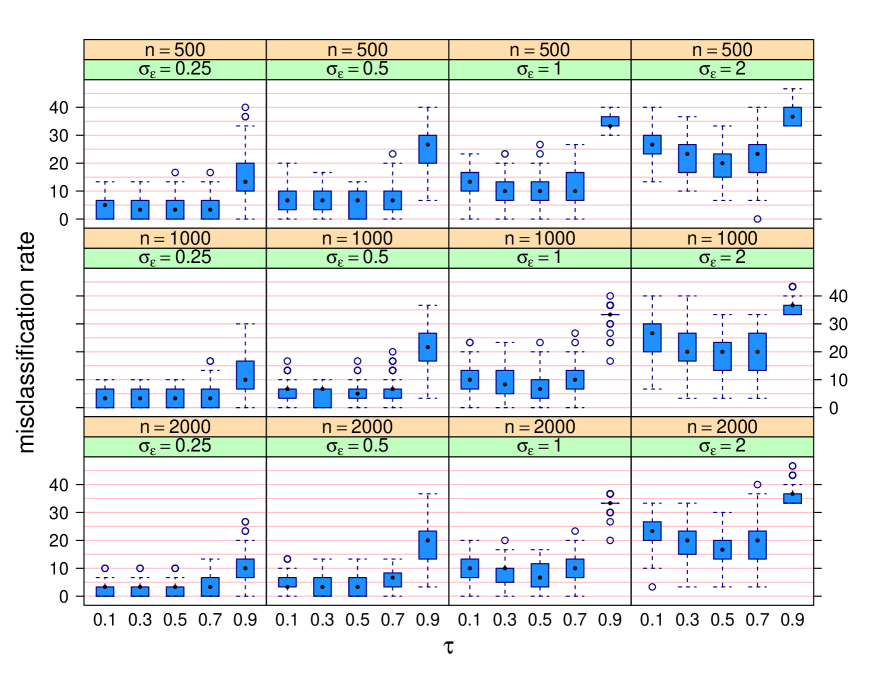
Figure 3: Side-by-side boxplots of the misclassification rates for the Markov chain Monte Carlo Algorithm 2 for the simulation study described in the text. Each panel corresponds to a different combination of sample size and error standard deviation. Within each panel, the side-by-side boxplots compare misclassification rate as a function of the threshold parameter $\tau$.

The analogous results for the mean field variational Bayes approach of Algorithm 3 are shown in Figure 4. This time the boxplots indicate better performance for $\tau<0.5$. We conjecture that mean field approximations have a detrimental effect on the $\tau={\textstyle{\frac{1}{2}}}$ decision rules and, for reasons yet to be understood, are somewhat remedied by setting $\tau$ to be a lower value such as $0.1$. Additional checks, not shown here, indicate the the classification performance gets worse for $\tau$ smaller than $0.1$ for this simulation set-up. Acknowledging the limitations of a single simulation study, our recommended default for $\tau$ in the mean field variational Bayes case is $\tau=0.1$.

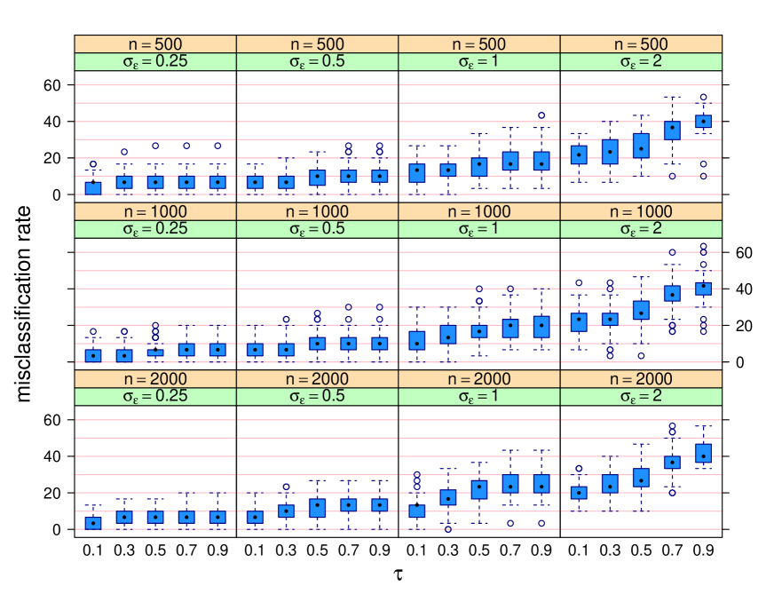
Figure 4: Side-by-side boxplots of the misclassification rates for the mean field variational Bayes Algorithm 3 for the simulation study described in the text. Each panel corresponds to a different combination of sample size and error standard deviation. Within each panel, the side-by-side boxplots compare misclassification rate as a function of the threshold parameter $\tau$.

We also ran simulation studies for the Bernoulli response case, with a similar design to the Gaussian study. The recommendations of $\tau=0.5$ for Markov chain Monte Carlo and $\tau=0.1$ for mean field variational Bayes were also supported by that study.

Additional simulation studies, involving an alternative evaluation metric and hyperparameter sensitivity checks, are given in Section S.3. These studies do not alter any of our recommendations concerning the choice of $\tau$.

3.6 Package in the R Language

The R package gamselBayes (He & Wand, 2023) implements Algorithms 2 and 3 and provides tabular and graphical summaries of selected generalized additive models. Speed is enhanced via C++ implementation of the loops in the two algorithms. The gamselBayes package is available on the Comprehensive R Archive Network (https://www.R-project.org). The gamselBayes package is accompanied by a vignette which provides fuller details on its use. The vignette PDF file is opened via the command gamselBayesVignette().

4 Comparative Performance

We ran a second simulation study to assess comparative performance of the new methodology with respect to some of the other existing approaches to three-category generalized additive model selection. The simulation design was the same as that described in Section 3.5.3. In keeping with the findings of that section, in Algorithm 2 the threshold parameter was set to $\tau=0.5$ and for Algorithm 3 it was set to $\tau=0.1$.

The other approaches considered were those used by the R packages:

1. spikeSlabGAM (Scheipl, 2022), which is a Bayesian approach that is described in Scheipl et al. (2012). Details on use of the spikeSlabGAM package are given in Scheipl (2011).

2. gamsel (Chouldechova & Hastie, 2022), which implements the frequentist approach described in Chouldechova & Hastie (2015). The package’s main function, cv.gamsel(), computes a family of generalized additive model fits over a grid of regularization parameter values. For selection of a single model, cv.gamsel() provides the option of minimizing a $k$-fold cross-validation function over the grid.

The Bernoulli response versions of these approaches involve the logit link function, rather than the probit link function used by Algorithms 2 and 3. This necessitated use of the appropriate inverse link transformation for the generation of binary response data in this simulation study.

In the case of spikeSlabGAM, we used the default call to its spikeSlabGAM() function. The model having highest posterior probability in the spikeSlabGAM() output object was selected. The essential difference between spikeSlabGAM and Algorithms 2 and 3 is the form of the prior distributions imposed on the coefficients for the linear and spline components. In the notation of Section 2.4, spikeSlabGAM replaces (6) by

$$\mathfrak{p}(\beta|\sigma_{\mbox{\tiny{$\beta$}}},\rho_{\mbox{\tiny{$\beta$}}})=\frac{\rho_{\mbox{\tiny{$\beta$}}}\exp\big{\{}-\beta^{2}/(2\sigma_{\mbox{\tiny{$\beta$}}}^{2})\big{\}}}{(2\pi\sigma_{\mbox{\tiny{$\beta$}}}^{2})^{1/2}}+\frac{(1-\rho_{\mbox{\tiny{$\beta$}}})\exp\big{[}-\beta^{2}/\{2(v_{0}\sigma_{\mbox{\tiny{$\beta$}}})^{2}\}\big{]}}{\{2\pi(v_{0}\sigma_{\mbox{\tiny{$\beta$}}})^{2}\}^{1/2}}\quad\mbox{where}\quad v_{0}\ll 1$$ (17)

with $v_{0}$ having a default value of $0.00025$. Note (17) is an alternative to the “spike-and-slab” prior used by (6), with the “slab” being Gaussian rather than Laplacian and the default “spike” being a $N(0,0.00025^{2})$ mass rather than the point mass at zero. For spline coefficient vectors, the alternative to (7) used by spikeSlabGAM is an extension of (17) that is described by Figure 1 of Scheipl (2011) and accompanying text. For Gaussian response models spikeSlabGAM uses Gibbs sampling, but requires Metropolis-Hastings sampling for non-Gaussian responses.

Preliminary checks revealed that default regularization grid used by cv.gamsel() did not lead to very good three-category classification performance, with the cross-validation mean function often being monotonic rather than U-shaped. To circumvent this apparent default grid problem, with respect to the three-category misclassification rate, we experimented with its choice and found that geometric sequence of size $50$ between $0.01$ and $2$ usually lead to U-shaped cross-validation mean functions for the simulation settings. This regularization grid was used throughout the comparative performance simulation study with $10$-fold cross-validation for model selection. Two cross-validation-based choices were considered: the regularization parameter matching the absolute minimum of the mean values, and largest regularization parameter value such that mean minus one standard deviation is below the absolute minimum. However, after running the simulation study it was found that the three-category misclassification rates for the gamsel approaches were considerably higher than the other approaches since it has a tendency to choose larger models. Given this poor performance for misclassification rate, relative to the other methods in the study, the gamsel results are excluded from the upcoming graphical summaries (Figures 5 and 6).

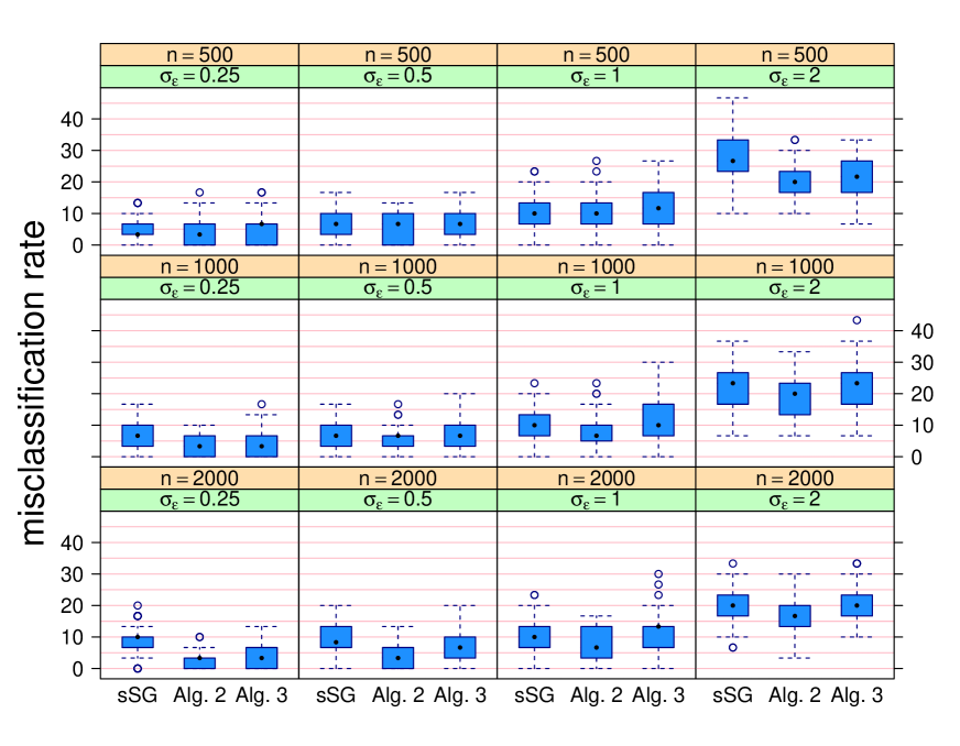
Figure 5: Side-by-side boxplots of the misclassification rates for the comparative performance simulation study described in the text in the case of the response variable being Gaussian. Each panel corresponds to a different combination of sample size and error standard deviation. Within each panel, the side-by-side boxplots compare misclassification rate across each of three methods: spikeSlabGAM with default settings (sSG), Algorithm 2 (Alg. 2) and Algorithm 3 (Alg. 3).

Figure 5 shows the misclassification rates for Algorithms 2 and 3 in comparison with the default version of the spikeSlabGAM approach as side-by-side boxplots for the Gaussian response case. In the lower error standard deviation situations, all have similar performance. The fast variational approach of Algorithms 3 is seen to have lower accuracy when the noise level is higher. This degradation in performance needs to be mitigated against run time, which is addressed later in this section.

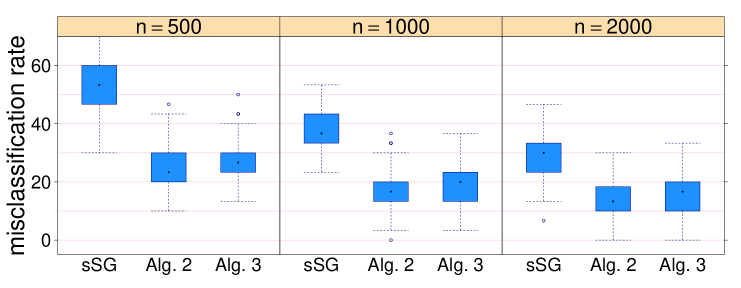
Figure 6: Side-by-side boxplots of the misclassification rates for the comparative performance simulation study described in the text in the case of the response variable being binary. Each panel corresponds to a different combination of sample size and error standard deviation. Within each panel, the side-by-side boxplots compare misclassification rate across each of three methods: spikeSlabGAM with default settings (sSG), Algorithm 2 (Alg. 2) and Algorithm 3 (Alg. 3).

The binary response simulation results are shown in Figure 6. Algorithms 2 and 3 are seen to have better three-category classification performance compared with spikeSlabGAM for the binary response simulation study.

Lastly, we report on the computing times for the four approaches. Specifically, these are elapsed times in seconds for each generalized additive model selection on a MacBook Air laptop computer with 16 gigabytes of memory and a 3.2 gigahertz processor. Algorithms 2 and 3 were implemented using the Rcpp interface (Eddelbuettel & François, 2011) to the C++ language. The Markov chain Monte Carlo sample size values corresponded to the spikeSlabGAM and gamselBayes defaults of $1,500$ and $2,000$ respectively. Table 2 lists the 10th, 50th and 90th percentile number of seconds for each approach across all settings and replications.

	gamsel	spikeSlabGAM	Algorithm 2	Algorithm 3
10th percentile	3.69	84.9	1.78	0.326
50th percentile	8.12	167.0	2.14	0.466
90th percentile	17.50	339.0	3.03	0.768

Table 2: 10th, 50th and 90th percentiles for the number of seconds required for each generalized additive model selection approach across all settings and replications for the comparative performance simulation study.

It is apparent from Table 2 that, despite exhibiting very good classification, spikeSlabGAM is comparatively slow and does not scale well to large problems. Algorithm 2 took less than around 3 seconds for 90% of the fits in the simulation study. The faster variational approach of Algorithm 3 only required less than a second of computing time for most of the fits. Therefore, the new approaches have very good scalability for the generalized additive model selection problem.

The impact of sample size and number of candidate predictors on computing times for Algorithms 2 and 3 is investigated in Section S.3.2.

5 Data Illustrations

We finish off with two illustrations for actual data. Both illustrations involve binary responses. The first one is a relative small problem, where Markov chain Monte Carlo fitting of the binary response adjustment of (9) is quick. The second example involves a much bigger data set, and mean field variational Bayes offers relatively fast model selection.

5.1 Application to Mortgage Applications Data

Data originating from the Federal Bank of Boston, U.S.A., has $2,380$ records on mortgage applications, and is available in the R data package Ecdat (Croissant, 2022) as a data frame titled Hmda. The response variable is the indicator of whether the mortgage application was denied. After conversion of each of the categorical variables to indicator form there are 20 candidate predictors. Fourteen of these candidate predictors are binary, so can only be considered as having a zero or linear effect. The remaining four predictors are continuous, and three of these were considered as having zero, linear or non-linear effects. One of them, corresponding to the unemployment rate of the industry corresponding to the applicant’s occupation, has only 10 unique values and penalized spline models have borderline viability. Therefore, the effect of this predictor was restricted to zero versus linear.

Application of Algorithm 2 and the effect type estimation rules of Section 3.5 with $\tau=0.5$ led to the estimated effect types listed in Table 3. Markov chain Monte Carlo sampling involved a warm-up of length $1,000$ and $1,000$ retained samples used for inference. Chain diagnostic graphics, including trace, lag-1 and autocorrelation function plots, indicated good convergence. The vignette attached to the gamselBayes package includes these diagnostic graphics.

candidate predictor	est. type		candidate predictor	est. type
bad public credit record?	linear		credit score of 3?	zero
denied mortgage insurance?	linear		credit score of 4?	zero
applicant self-employed?	linear		credit score of 5?	zero
applicant single?	linear		mortgage credit score of 1?	zero
applicant black?	linear		mortgage credit score of 2?	zero
property a condominium?	zero		mortgage credit score of 3?	zero
unemploy. rate applic. indus.	zero		debt payments/income ratio	non-linear
credit score of 1?	linear		housing expenses/income ratio	zero
credit score of 2?	linear		loan size/property value ratio	non-linear

Table 3: Each of the candidate predictors for the Boston mortgage example and the estimated effect type from application of Algorithm 2 and effect type estimation rules of Section 3.5. The candidate predictors with question marks correspond to binary indicator variables. The abbreviation “unemploy. rate applic. indus.” stands for the unemployment rate of the industry corresponding to the applicant’s occupation.

As is apparent from Table 3, the selected model has 7 linear effects, 2 non-linear effects and 9 candidate predictors discarded. Table 4 provides estimation and inferential summaries for the linear effects.

predictor	posterior mean	95% credible interval
indicator of bad public credit record	$0.7350$	$(0.4926,0.9848)$
indicator of denied mortgage insurance	$2.7620$	$(2.1426,3.5172)$
indicator of applicant being single	$0.1370$	$(0.0000,0.3417)$
indicator of applicant being black	$0.3461$	$(0.0842,0.5404)$
indicator of applicant being self-employed	$0.1703$	$(0.0000,0.4363)$
indicator of credit score equalling 1	$-0.6906$	$(-0.8980,-0.4513)$
indicator of credit score equalling 2	$-0.3238$	$(-0.5869,0.0000)$

Table 4: Approximate posterior means and approximate 95% credible intervals for the coefficients of each of the selected linear fits based on the Markov chain Monte Carlo samples generated from Algorithm 2 for the Boston mortgages example.

Table 3 shows an applicant having bad public credit record is more likely to have their mortgage application denied, which is in keeping with financial commonsense. Of potential interest from a social justice standpoint is the significant effects on denial probability for applicants that are either black or single.

Figure 7 shows the two effects have non-linear effects in the selected model. The effect of debt payment to income ratio is quite a striking non-monotonic curve.

Figure 7: The two estimated non-linear effects for the Boston mortgage example from application of Algorithm 2 and effect type estimation rules of Section 3.5 with $\tau=0.5$. Each curve is the slice of estimated probability of mortgage denial as a function of the predictor, with all other selected predictors set to their median values. The shaded region corresponds to pointwise approximate 95% credible intervals.

5.2 Application to Car Auction Data

During 2011-2012 the kaggle Internet platform (https://www.kaggle.com) hosted a classification competition involving training data consisting of $49$ variables on $72,983$ cars purchased at automobile auctions by automobile dealerships in U.S.A. The title of the competition was “Don’t Get Kicked!”. A version of the data in which all categorical variables have been converted to binary variable indicator form is stored in the data frame carAuction within the R package HRW (Harezlak et al., 2021). The response variable is the indicator of whether the car purchased at auction by the dealership had serious problems that hinder or prevent it being sold. For short, we refer to such a car as a “bad buy”. Forty-four of the candidate predictors are binary. The other $5$ candidate predictors are continuous. However, the age at sale variable has only $10$ unique values. For the same reasons given for the unemployment rate variable considered in the Boston mortgages example, we exclude age at sale from having a non-linear effect.

Since this generalized additive model selection problem involves a relatively large sample size and number of candidate predictors, we use it to illustrate the fast variational approach corresponding to Algorithm 3. The mean field variational Bayes iterations described there were iterated until the relative change in the approximate marginal log-likelihood fell below $10^{-8}$. On the second author’s MacBook Air laptop, with a 3.2 gigahertz processor and 16 gigabytes of random access memory, mean field Bayes variational fitting took 11 seconds. The rules of Section 3.5 were applied with $\tau=0.1$. This resulted in $19$ predictors being selected as having a linear effect and $3$ predictors having non-linear effects. Twenty-seven of the $49$, or $55\%$, of candidate predictors were discarded.

Table 5 provides estimation and inferential summaries for the linear effects coefficients. Most of the predictor effects are intuitive, such as older cars being more likely to be a bad buy and presence of wheel covers lowering the bad buy probability. Some of them, such as the effect of cars being purchased in particular states, are more intriguing.

predictor	posterior mean	95% credible interval
indic. made in U.S.A.	$-0.04605$	$(-0.06925,-0.02323)$
age at sale (years)	$0.09344$	$(0.08771,0.09896)$
indic. color is red	$0.05130$	$(0.02498,0.07713)$
indic. make is Chevrolet	$-0.1103$	$(-0.1358,-0.08426)$
indic. make is Chrysler	$0.09517$	$(0.06910,0.1217)$
indic. make is Dodge	$-0.03093$	$(-0.05385,-0.006961)$
indic. purchased online	$-0.06229$	$(-0.1117,0.0000)$
acquisition price (U.S. dollars)	$-6.014\times 10^{-6}$	$(-9.352,-2.603)\times 10^{-6}$
indic. purchased in 2010	$0.1085$	$(0.09290,0.1242)$
indic. purch. in Florida	$-0.1173$	$(-0.1391,-0.09529)$
indic. purch. in North Carolina	$-0.1074$	$(-0.1326,-0.08190)$
indic. purch. in Texas	$0.09706$	$(0.07799,0.1162)$
indic. medium-sized vehicle	$-0.07368$	$(-0.09095,-0.05622)$
indic. sports utility vehicle	$0.1899$	$(0.1646,0.2153)$
indic. manual transmission	$-0.1574$	$(-0.1970,-0.1168)$
indic. trim level is ‘Bas’	$0.05521$	$(0.0355,0.07477)$
indic. trim level is ‘LS’	$-0.06153$	$(-0.09180,-0.03176)$
indic. has alloy wheels	$-1.513$	$(-1.546,-1.480)$
indic. has wheel covers	$-1.585$	$(-1.619,-1.551)$

Table 5: Approximate posterior means and approximate 95% credible intervals for the coefficients of each of the selected linear fits based on the mean field variational Bayes optimal $\mathfrak{q}$-densities obtained from Algorithm 3 for the car auction example.

Figure 8 shows the three selected non-linear effects, which are the impacts of the probability of a bad buy as functions of the odometer reading in miles, acquisition cost paid for the car at the time of purchase in U.S. dollars and warranty cost in U.S. dollars. The middle panel of Figure 8 shows that a cost of about $10,000$ U.S. dollars is best, and that the probability of bad buy increases when the cost deviates away from this amount. The shaded regions of Figure 8 corresponds to pointwise approximate 95% credible intervals. However, for a binary response model such as this, there is considerable mean field approximation error which tends to make the credible intervals overly narrow.

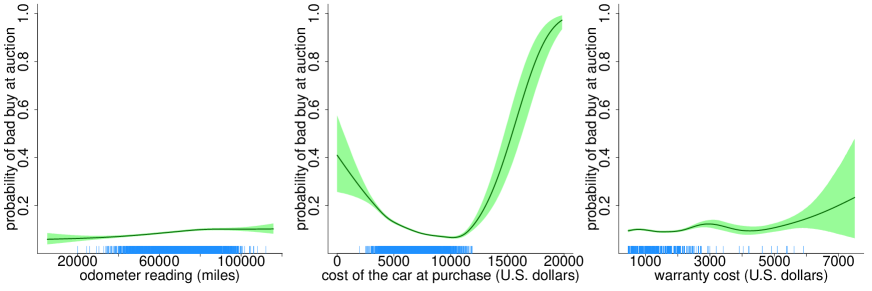
Figure 8: The estimated non-linear effects for the car auction example from application of Algorithm 3 and effect type estimation rules of Section 3.5 with $\tau=0.1$. The curves are slices of estimated probability of bad buy as a function of the predictor, with all other selected predictors set to their median values. The shaded regions correspond to pointwise approximate 95% credible intervals, but are subject to considerable mean field approximation error. The rug at the base of each plot is based on a random sample of $2,500$ cars.

As a type of check, we also applied the Markov chain Monte Carlo Algorithm 2 to the same data set. This resulted in 14 of the 19 predictors in Table 5 being selected. Three predictors not selected by Algorithm 3, such as indicators of the auction provider, were selected by Algorithm 2. The odometer reading predictor was estimated to have a non-linear effect by Algorithm 3, but to have a linear effect by Algorithm 2. In summary, Algorithm 3 selected 22 predictors whilst Algorithm 2 selected 20 predictors with 17 predictors in common from the two approaches. This suggests reasonable accuracy of the faster variational approach for this example.

6 Concluding Remarks

The methodology conveyed by Algorithms 1–3 and the effect type classification rules given in Sections 3.5.1 and 3.5.2 represent a practical Bayesian alternative to the frequentist methodology of Chouldechova & Hastie (2015) for three-category generalized additive model selection. Both approaches are driven by the goals of speed and scalability to large data sets. The new Bayesian approach is the clear winner in terms of accuracy according to our simulation studies.

Our, admittedly limited, simulation studies indicate improved classification performance compared with default use of spikeSlabGAM in binary response situations. In the Gaussian response situations the performance of Algorithm 2 and spikeSlabGAM is similar, with Algorithm 3 falling behind for higher noise situations. This needs to be mitigated against the vastly improved speed and scalability, as indicated by Table 2, of this article’s new methodologies. The best approach in practice depends on data set size and time demands, with the simulation results of Sections 3 and 4 providing some guidance. Additional simulation results are given in Section S.3 of the supplement.

Disclosure Statement

The authors report that there are no competing interests to declare.

References

Albert, J.H. & Chib, S. (1993). Bayesian analysis of binary and polychotomous response data. Journal of the American Statistical Association, 88, 669–679.

Azzalini, A. (2023). sn 2.1.1: The Skew-Normal and related distributions such as the Skew-t and the Unified Skew-Normal. R package.
http://azzalini.stat.unipd.it/SN

Bhadra, A., Datta, J., Polson, N.G. & Willard, B. (2019). Lasso meets horseshoe: a survey. Statistical Science, 34, 405–427.

Bürkner, P.-C. (2022). bmrs 2.18.0: Bayesian regression models using Stan. R package.
https://r-project.org

Carvalho, C.M., Polson, N.G. & Scott, J.G. (2010). The horseshoe estimator for sparse signals. Biometrika, 97, 465–480.

Chouldechova, A. & Hastie, T. (2015). Generalized additive model selection.
https://arXiv.org/abs/1506.03850v2

Chouldechova, A. & Hastie, T. (2022). gamsel 1.8: Fit regularization path for generalized additive models. R package. https://r-project.org

Croissant, Y. (2022). Ecdat 0.4: Data sets for econometrics. R package.
https://r-project.org

Eddelbuettel, D. & François, R. (2011). Rcpp: Seamless R and C++ integration. Journal of Statistical Software, 40(8), 1–18.

Gelfand, A.E. & Smith, A.F.M. (1990). Sampling-based approaches to calculating marginal densities. Journal of the American Statistical Association, 85, 398–409.

Gelman, A. (2006). Prior distributions for variance parameters in hierarchical models. Bayesian Analysis, 1, 515–533.

George & McCulloch, R.E. (1993). Variable selection via Gibbs sampling. Journal of the American Statistical Association, 88, 881–889.

Griffin, J.E. & Brown, P.J. (2011). Bayesian hyper-lassos with non-convex penalization. Australian and New Zealand Journal of Statistics, 53, 423–442.

Harezlak, J., Ruppert, D. & Wand, M.P. (2021). HRW 1.0: Datasets, functions and scripts for semiparametric regression supporting Harezlak, Ruppert & Wand (2018). R package. https://r-project.org

Hastie, T.J. & Tibshirani, R.J. (1990). Generalized Additive Models. New York: Chapman & Hall.

He, V.X. & Wand, M.P. (2023). gamselBayes: Bayesian generalized additive model selection. R package version 2.0.
http://cran.r-project.org.

Ishwaran, H. & Rao, J.S. (2005). Spike and slab variable selection: frequentist and Bayesian strategies. The Annals of Statistics, 33, 730–733.

Kyung, M., Gill, J., Ghosh, M. & Casella, G. (2010). Penalized regression, standard errors, and Bayesian lassos. Bayesian Analysis, 5, 369–412.

Lempers, F.B. (1971). Posterior Probabilities of Alternative Linear Models. Rotterdam: Rotterdam University Press.

Michael, J.R., Schucany, W.R. & Haas, R.W. (1976). Generating random variates using transformations with multiple roots. The American Statistician, 30, 88–90.

Mitchell, T.J. & Beauchamp, J.J. (1988). Bayesian variable selection in linear regression. Journal of the American Statistical Association, 83, 1023–1032.

Ngo, L. and Wand, M.P. (2004). Smoothing with mixed model software. Journal of Statistical Software, 9, Article 1, 1–54.

Ormerod, J.T. and Wand, M.P. (2010). Explaining variational approximations. The American Statistician, 64, 140–153.

Park, T. & Casella, G. (2008). The Bayesian Lasso. Journal of the American Statistical Association, 103, 681–686.

Ravikumar, P., Lafferty, J., Liu, H. & Wasserman, L. (2009). Sparse additive models. Journal of the Royal Statistical Society, Series B, 71, 1009–1030.

R Core Team (2023). R: A language and environment for statistical computing. R Foundation for Statistical Computing, Vienna, Austria. https://www.r-project/org/.

Reich, B.J., Sorlie, C.B. & Bondell, H.D. (2009). Variable selection in smoothing spline ANOVA: application to deterministic computer codes. Technometrics, 51, 110–120.

Robert, C.P. (1995). Simulation of truncated normal variates. Statistics and Computing, 5, 121–125.

Scheipl, F. (2011). spikeSlabGAM: Bayesian variable selection, model choice and regularization for generalized additive mixed models in R. Journal of Statistical Software, 43, Issue 14. 1–24.

Scheipl, F. (2022). spikeSlabGAM 1.1: Bayesian variable selection and model choice for generalized additive mixed models. R package.
https://github.com/fabian-s/spikeSlabGAM

Scheipl, F., Fahrmeir, L. & Kneib, T. (2012). Spike-and-slab priors for function selection in structured additive regression models. Journal of the American Statistical Association, 107, 1518–1532.

Shively, T.S., Kohn, R. & Wood, S. (1999). Variable selection and function estimation in additive nonparametric regression using a data-based prior. Journal of the American Statistical Association, 94, 777–794.

Umlauf, N., Klein, N., Zeileis, A. & Simon, T. (2023). bamlss 1.2: Bayesian additive models for location, scale, and shape (and beyond). R package. https://www.bamlss.org

Umlauf, N., Kneib, T. & Klein, N. (2023). BayesX 0.3: R utilities accompanying the software package BayesX. R package. https://www.BayesX.org

Wainwright, M.J. & Jordan, M.I. (2008). Graphical models, exponential families and variational inference. Foundations and Trends in Machine Learning, 1, 1–305.

Wand, M.P. & Ormerod, J.T. (2008). On semiparametric regression with O’Sullivan penalized splines. Australian and New Zealand Journal of Statistics, 50, 179–198.

Wand, M.P. and Ormerod, J.T. (2011). Penalized wavelets: embedding wavelets into semiparametric regression. Electronic Journal of Statistics, 5, 1654–1717.

Wand, M.P. and Ormerod, J.T. (2012). Continued fraction enhancement of Bayesian computing. Stat, 1, 31–41.

Wood, S.N. (2017). Generalized Additive Models: An Introduction with R, Second Edition, Boca Raton, Florida: CRC Press.

Yuan, M. & Lin, Y. (2006). Model selection and estimation in regression with grouped variables. Journal of the Royal Statistical Society, Series B, 68, 49–67.

Supplement for:

Bayesian Generalized Additive Model Selection

Including a Fast Variational Option

By Virginia X. He and Matt P. Wand

University of Technology Sydney

S.1 The Canonical Demmler-Reinsch Spline Basis

Let $\boldsymbol{x}=(x_{1},\ldots,x_{n})$ be a continuous univariate data set. In the context of this article, the $x_{i}$s correspond to values of a continuous candidate predictor. Let $[a,b]$ be an interval containing the $x_{i}$s. For an integer $K\leq n-2$, let $\boldsymbol{\kappa}_{\mbox{\tiny inter.}}\equiv(\kappa_{1},\ldots,\kappa_{K-2})$ be a set of so-called interior knots such that

$$a<\kappa_{1}<\cdots<\kappa_{K-2}<b.$$

A reasonable default value for $K$ is around $30$, or smaller values if the number of unique $x_{i}$s is lower. It is common to place the interior knots at sample quantiles of the $x_{i}$s.

We now list steps for construction of the matrix $\boldsymbol{Z}$ containing canonical Demmler-Reinsch basis functions of the entries of $\boldsymbol{x}$. The justification for Steps (3)–(6) is given in Section 9.1.1 of Ngo & Wand (2004).

• Use the steps described in Section 4 of Wand & Ormerod (2008) to obtain the matrix denoted by $\boldsymbol{Z}$ in that section’s equation (6), which contains canonical O’Sullivan spline basis functions. Denote this matrix by $\boldsymbol{Z}_{\mbox{\tiny OS}}$ and note that it has dimension $n\times K$.

• Form the matrix $\boldsymbol{C}_{\mbox{\tiny OS}}=[\boldsymbol{1}_{n}\ \boldsymbol{x}\ \boldsymbol{Z}_{\mbox{\tiny OS}}]$ and set $\boldsymbol{D}=\mbox{diag}(0,0,\boldsymbol{1}_{K})$.

• Obtain the singular value decomposition of $\boldsymbol{C}_{\mbox{\tiny OS}}$:

  $$\boldsymbol{C}_{\mbox{\tiny OS}}=\boldsymbol{U}_{\mbox{\tiny{$C$}}}\mbox{diag}(\boldsymbol{d}_{\mbox{\tiny{$C$}}})\boldsymbol{V}_{\mbox{\tiny{$C$}}}^{T}\ \mbox{where $\boldsymbol{U}_{\mbox{\tiny{$C$}}}$ is $n\times(K+2)$ and $\boldsymbol{V}_{\mbox{\tiny{$C$}}}$ is $(K+2)\times(K+2)$}$$

  $$\mbox{such that}\ \boldsymbol{U}_{\mbox{\tiny{$C$}}}^{T}\boldsymbol{U}_{\mbox{\tiny{$C$}}}=\boldsymbol{V}_{\mbox{\tiny{$C$}}}^{T}\boldsymbol{V}_{\mbox{\tiny{$C$}}}=\boldsymbol{I}_{K+2}.$$

• Form the symmetric matrix $\mbox{diag}(\boldsymbol{1}/\boldsymbol{d}_{\mbox{\tiny{$C$}}})\boldsymbol{V}_{\mbox{\tiny{$C$}}}^{T}\boldsymbol{D}\boldsymbol{V}_{\mbox{\tiny{$C$}}}\mbox{diag}(\boldsymbol{1}/\boldsymbol{d}_{\mbox{\tiny{$C$}}})$ and obtain its singular value decomposition:

  $$\mbox{diag}(\boldsymbol{1}/\boldsymbol{d}_{\mbox{\tiny{$C$}}})\boldsymbol{V}_{\mbox{\tiny{$C$}}}^{T}\boldsymbol{D}\boldsymbol{V}_{\mbox{\tiny{$C$}}}\mbox{diag}(\boldsymbol{1}/\boldsymbol{d}_{\mbox{\tiny{$C$}}})=\boldsymbol{U}_{\mbox{\tiny{$D$}}}\mbox{diag}(\boldsymbol{d}_{\mbox{\tiny{$D$}}})\boldsymbol{V}_{\mbox{\tiny{$D$}}}^{T}\ \mbox{where $\boldsymbol{U}_{\mbox{\tiny{$D$}}}$ is $(K+2)\times(K+2)$}$$

  $$\mbox{and $\boldsymbol{V}_{\mbox{\tiny{$D$}}}$ is $(K+2)\times(K+2)$ such that}\ \boldsymbol{U}_{\mbox{\tiny{$D$}}}^{T}\boldsymbol{U}_{\mbox{\tiny{$D$}}}=\boldsymbol{V}_{\mbox{\tiny{$D$}}}^{T}\boldsymbol{V}_{\mbox{\tiny{$D$}}}=\boldsymbol{I}_{K+2}.$$

• Set the full (non-canonical) Demmler-Reinsch matrix as follows: $\boldsymbol{C}_{\mbox{\tiny DR}}\longleftarrow\boldsymbol{U}_{\mbox{\tiny{$C$}}}\boldsymbol{U}_{\mbox{\tiny{$D$}}}$.

• The next steps assume that the singular value decompositions follow the convention that $\boldsymbol{d}_{\mbox{\tiny{$D$}}}$ is a $(K+2)\times 1$ vector with its entries in non-increasing order. Adjustments to the singular value decompositions are needed if this convention is not used.

• Set the $(K+2)\times 1$ vector $\boldsymbol{s}_{\mbox{\tiny{$D$}}}$ as follows:

  $$\omega_{21}\longleftarrow\sqrt{\mbox{$K$th entry of $\boldsymbol{d}_{\mbox{\tiny{$D$}}}$}},\ \ \ ;\ \ \ \boldsymbol{s}_{\mbox{\tiny{$D$}}}\longleftarrow\omega_{21}\boldsymbol{1}_{K+2}\Big{/}\sqrt{\boldsymbol{d}_{\mbox{\tiny{$D$}}}}$$

  and then set the last two entries of $\boldsymbol{s}_{\mbox{\tiny{$D$}}}$ to equal $1$.

• Set the full canonical Demmler-Reinsch design matrix as follows:

  $$\boldsymbol{C}_{\mbox{\tiny cDR}}\longleftarrow\boldsymbol{C}_{\mbox{\tiny DR}}\mbox{diag}(\boldsymbol{s}_{\mbox{\tiny{$D$}}}).$$

• Set the O’Sullivan to canonical Demmler-Reinsch transformation matrix as follows:

  $$\boldsymbol{L}_{\mbox{\tiny OS.to.cDR}}\longleftarrow\boldsymbol{V}_{\mbox{\tiny{$C$}}}\mbox{diag}(\boldsymbol{1}/\boldsymbol{d}_{\mbox{\tiny{$C$}}})\boldsymbol{U}_{\mbox{\tiny{$D$}}}\mbox{diag}(\boldsymbol{s}_{\mbox{\tiny{$D$}}}).$$

  This $(K+2)\times(K+2)$ matrix has the following property:

  $$\boldsymbol{C}_{\mbox{\tiny OS}}\boldsymbol{L}_{\mbox{\tiny OS.to.cDR}}=\boldsymbol{C}_{\mbox{\tiny cDR}}$$

  and is useful for prediction and plotting purposes. This is because grid-wise analogues of $\boldsymbol{C}_{\mbox{\tiny OS}}$ are readily computed using the structures described in Wand & Ormerod (2008) involving cubic B-spline basis functions.

• Reverse the order of the columns of $\boldsymbol{C}_{\mbox{\tiny cDR}}$. Reverse the order of the columns of $\boldsymbol{L}_{\mbox{\tiny OS.to.cDR}}$.

• The matrix containing canonical spline basis functions of the inputs $\boldsymbol{x}$ and $\boldsymbol{\kappa}_{\mbox{\tiny inter.}}$ is

  $$\boldsymbol{Z}\longleftarrow\mbox{the $n\times K$ matrix consisting of columns $3$ to $K+2$ of $\boldsymbol{C}_{\mbox{\tiny cDR}}$.}$$

A function in the R language for computing $\boldsymbol{Z}$ and $\boldsymbol{L}_{\mbox{\tiny OS.to.cDR}}$ for given $\boldsymbol{x}$ and $\boldsymbol{\kappa}_{\mbox{\tiny inter.}}$ can be accessed by downloading the accompanying gamselBayes package. Assuming that the gamselBayes package is installed, the relevant function is gamselBayes:::ZcDR().

S.2 Approximate Marginal Log-Likelihood Expressions

The approximate marginal log-likelihood is

$$\log\underline{p}(\boldsymbol{y};\mathfrak{q})=\left\{\begin{array}[]{lcl}\log\underline{p}(\boldsymbol{y};\mathfrak{q},\mbox{C})+E_{\mathfrak{q}}[\log\{\mathfrak{p}(\boldsymbol{y}|\beta_{0},\gamma_{\mbox{\tiny{$\beta$}}},{\widetilde{\boldsymbol{\beta}}},\gamma_{\mbox{\tiny{$u$}}},{\widetilde{\boldsymbol{u}}},\sigma_{\varepsilon}^{2})\}]\\[4.30554pt] \quad+E_{\mathfrak{q}}[\log\{\mathfrak{p}(\sigma_{\varepsilon}^{2}|a_{\varepsilon})\}]-E_{\mathfrak{q}}[\log\{\mathfrak{q}(\sigma_{\varepsilon}^{2})\}]\\[4.30554pt] \quad+E_{\mathfrak{q}}[\log\{\mathfrak{p}(a_{\varepsilon})\}]-E_{\mathfrak{q}}[\log\{\mathfrak{q}(a_{\varepsilon})\}]&\mbox{Gaussian response case,}\\[8.61108pt] \log\underline{p}(\boldsymbol{y};\mathfrak{q},\mbox{C})+E_{\mathfrak{q}}[\log\{\mathfrak{p}(\boldsymbol{y}|\boldsymbol{c})\}]\\[4.30554pt] \quad+E_{\mathfrak{q}}[\log\{\mathfrak{p}(\boldsymbol{c}|\beta_{0},\gamma_{\mbox{\tiny{$\beta$}}},{\widetilde{\boldsymbol{\beta}}},\gamma_{\mbox{\tiny{$u$}}},{\widetilde{\boldsymbol{u}}})\}]-E_{\mathfrak{q}}[\log\{\mathfrak{q}(\boldsymbol{c})\}]&\mbox{Bernoulli response case,}\end{array}\right.$$

where

$${\begin{array}[]{rcl}&&\log\underline{p}(\boldsymbol{y};\mathfrak{q},\mbox{C})=E_{\mathfrak{q}}[\log\{\mathfrak{p}(\beta_{0})\}]-E_{\mathfrak{q}}[\log\{\mathfrak{q}(\beta_{0})\}]+E_{\mathfrak{q}}[\log\{\mathfrak{p}(\gamma_{\mbox{\tiny{$\beta$}}})\}]-E_{\mathfrak{q}}[\log\{\mathfrak{q}(\gamma_{\mbox{\tiny{$\beta$}}})\}]\\[4.30554pt] &&\qquad+E_{\mathfrak{q}}[\log\{\mathfrak{p}({\widetilde{\boldsymbol{\beta}}}|\boldsymbol{b}_{\mbox{\tiny{$\beta$}}},\sigma^{2}_{\mbox{\tiny{$\beta$}}})\}]-E_{\mathfrak{q}}[\log\{\mathfrak{q}({\widetilde{\boldsymbol{\beta}}})\}]+E_{\mathfrak{q}}[\log\{\mathfrak{p}(\boldsymbol{b}_{\mbox{\tiny{$\beta$}}})\}]-E_{\mathfrak{q}}[\log\{\mathfrak{q}(\boldsymbol{b}_{\mbox{\tiny{$\beta$}}})\}]\\[4.30554pt] &&\qquad+E_{\mathfrak{q}}[\log\{\mathfrak{p}(\sigma^{2}_{\mbox{\tiny{$\beta$}}}|a_{\mbox{\tiny{$\beta$}}})\}]-E_{\mathfrak{q}}[\log\{\mathfrak{q}(\sigma^{2}_{\mbox{\tiny{$\beta$}}})\}]+E_{\mathfrak{q}}[\log\{\mathfrak{p}(a_{\mbox{\tiny{$\beta$}}})\}]-E_{\mathfrak{q}}[\log\{\mathfrak{q}(a_{\mbox{\tiny{$\beta$}}})\}]\\[4.30554pt] &&\qquad+E_{\mathfrak{q}}[\log\{\mathfrak{p}(\gamma_{\mbox{\tiny{$u$}}})\}]-E_{\mathfrak{q}}[\log\{\mathfrak{q}(\gamma_{\mbox{\tiny{$u$}}})\}]+E_{\mathfrak{q}}[\log\{\mathfrak{p}({\widetilde{\boldsymbol{u}}}|\boldsymbol{b}_{\mbox{\tiny{$u$}}},\boldsymbol{\sigma}_{\mbox{\tiny{$u$}}}^{2})\}]-E_{\mathfrak{q}}[\log\{\mathfrak{q}({\widetilde{\boldsymbol{u}}})\}]\\[4.30554pt] &&\qquad+E_{\mathfrak{q}}[\log\{\mathfrak{p}(\boldsymbol{b}_{\mbox{\tiny{$u$}}})\}]-E_{\mathfrak{q}}[\log\{\mathfrak{q}(\boldsymbol{b}_{\mbox{\tiny{$u$}}})\}]+E_{\mathfrak{q}}[\log\{\mathfrak{p}(\boldsymbol{\sigma}_{\mbox{\tiny{$u$}}}^{2}|\boldsymbol{a}_{\mbox{\tiny{$u$}}})\}]-E_{\mathfrak{q}}[\log\{\mathfrak{q}(\boldsymbol{\sigma}_{\mbox{\tiny{$u$}}}^{2})\}]\\[4.30554pt] &&\qquad+E_{\mathfrak{q}}[\log\{\mathfrak{p}(\boldsymbol{a}_{\mbox{\tiny{$u$}}})\}]-E_{\mathfrak{q}}[\log\{\mathfrak{q}(\boldsymbol{a}_{\mbox{\tiny{$u$}}})\}].\end{array}}$$ (S.1)

Here “C” signifies the fact that (S.1) is common to both $\log\underline{p}(\boldsymbol{y};\mathfrak{q})$ expressions.

Explicit expressions for $\log\underline{p}(\boldsymbol{y};\mathfrak{q})$ can be obtained by simplifying each of the $\mathfrak{q}$-density moment expressions. For example, the first term of (S.1) is

$$E_{\mathfrak{q}}[\log\{\mathfrak{p}(\beta_{0})\}] = -{\textstyle{\frac{1}{2}}}\log(2\pi)-{\textstyle{\frac{1}{2}}}\log(\sigma_{\beta_{0}}^{2})-{\textstyle{\frac{1}{2}}}E_{\mathfrak{q}}(\beta_{0}^{2})\big{/}\sigma_{\beta_{0}}^{2}$$

$$= -{\textstyle{\frac{1}{2}}}\log(2\pi)-{\textstyle{\frac{1}{2}}}\log(\sigma_{\beta_{0}}^{2})-{\textstyle{\frac{1}{2}}}\{\mu^{2}_{\mathfrak{q}(\beta_{0})}+\sigma^{2}_{\mathfrak{q}(\beta_{0})}\}\big{/}\sigma_{\beta_{0}}^{2}.$$

Also, since $\mathfrak{q}(\beta_{0})$ is the $N\big{(}\mu_{\mathfrak{q}(\beta_{0})},\sigma_{\mathfrak{q}(\beta_{0})}^{2}\big{)}$ density function, the second term of (S.1) is

$$-E_{\mathfrak{q}}[\log\{\mathfrak{q}(\beta_{0})\}] = {\textstyle{\frac{1}{2}}}\log(2\pi)+{\textstyle{\frac{1}{2}}}\log\big{(}\sigma_{\mathfrak{q}(\beta_{0})}^{2}\big{)}+{\textstyle{\frac{1}{2}}}E_{\mathfrak{q}}\big{\{}\big{(}\beta_{0}-\mu_{\mathfrak{q}(\beta_{0})}\big{)}^{2}\big{\}}\big{/}\sigma_{\mathfrak{q}(\beta_{0})}^{2}$$

$$= {\textstyle{\frac{1}{2}}}\{\log(2\pi)+1\}+{\textstyle{\frac{1}{2}}}\log\big{(}\sigma_{\mathfrak{q}(\beta_{0})}^{2}\big{)}.$$

Continuing in this fashion, and accounting for some cancellations, we obtain

$$\log\underline{p}(\boldsymbol{y};\mathfrak{q},\mbox{C}) = \mbox{const}_{1}-{\textstyle{\frac{1}{2}}}\{\mu^{2}_{\mathfrak{q}(\beta_{0})}+\sigma^{2}_{\mathfrak{q}(\beta_{0})}\}\big{/}\sigma_{\beta_{0}}^{2}+{\textstyle{\frac{1}{2}}}\log\big{(}\sigma_{\mathfrak{q}(\beta_{0})}^{2}\big{)}+\mbox{logit}(\rho_{\mbox{\tiny{$\beta$}}})\sum_{j=1}^{d_{\circ}+d_{\bullet}}\mu_{\mathfrak{q}(\gamma_{\mbox{\tiny{$\beta$}\scriptsize{$j$}}})}$$

$$\quad-\sum_{j=1}^{d_{\circ}+d_{\bullet}}\left[\mu_{\mathfrak{q}(\gamma_{\mbox{\tiny{$\beta$}\scriptsize{$j$}}})}\log\big{(}\mu_{\mathfrak{q}(\gamma_{\mbox{\tiny{$\beta$}\scriptsize{$j$}}})}\big{)}+\{1-\mu_{\mathfrak{q}(\gamma_{\mbox{\tiny{$\beta$}\scriptsize{$j$}}})}\}\log\big{(}1-\mu_{\mathfrak{q}(\gamma_{\mbox{\tiny{$\beta$}\scriptsize{$j$}}})}\big{)}\right]$$

$$\quad-{\textstyle{\frac{1}{2}}}\mu_{\mathfrak{q}(1/\sigma^{2}_{\mbox{\tiny{$\beta$}}})}\sum_{j=1}^{d_{\circ}+d_{\bullet}}\mu_{\mathfrak{q}(b_{\mbox{\tiny{$\beta$}\scriptsize{$j$}}})}\big{(}\mu_{\mathfrak{q}({\widetilde{\beta}}_{j})}^{2}+\sigma_{\mathfrak{q}({\widetilde{\beta}}_{j})}^{2}\big{)}+{\textstyle{\frac{1}{2}}}\log\big{|}\boldsymbol{\Sigma}_{\mathfrak{q}({\widetilde{\boldsymbol{\beta}}})}\big{|}$$

$$\quad-{\textstyle{\frac{1}{2}}}\sum_{j=1}^{d_{\circ}+d_{\bullet}}\{1/\mu_{\mathfrak{q}(b_{\mbox{\tiny{$\beta$}\scriptsize{$j$}}})}\}-\mu_{\mathfrak{q}(1/a_{\mbox{\tiny{$\beta$}}})}\mu_{\mathfrak{q}(1/\sigma^{2}_{\mbox{\tiny{$\beta$}}})}-{\textstyle{\frac{1}{2}}}(d_{\circ}+d_{\bullet}+1)\log\big{(}\lambda_{\mathfrak{q}(\sigma^{2}_{\mbox{\tiny{$\beta$}}})}\big{)}$$

$$\quad+\mu_{\mathfrak{q}(1/\sigma^{2}_{\mbox{\tiny{$\beta$}}})}\lambda_{\mathfrak{q}(\sigma^{2}_{\mbox{\tiny{$\beta$}}})}-\mu_{\mathfrak{q}(1/a_{\mbox{\tiny{$\beta$}}})}/s_{\mbox{\tiny{$\beta$}}}^{2}+\lambda_{\mathfrak{q}(a_{\mbox{\tiny{$\beta$}}})}\mu_{\mathfrak{q}(1/a_{\mbox{\tiny{$\beta$}}})}-\log\big{(}\lambda_{\mathfrak{q}(a_{\mbox{\tiny{$\beta$}}})})$$

$$\quad-\sum_{j=1}^{d_{\bullet}}\left[\mu_{\mathfrak{q}(\gamma_{\mbox{\scriptsize{$u$}\scriptsize{$j$}}})}\log\big{(}\mu_{\mathfrak{q}(\gamma_{\mbox{\scriptsize{$u$}\scriptsize{$j$}}})}\big{)}+\{1-\mu_{\mathfrak{q}(\gamma_{\mbox{\scriptsize{$u$}\scriptsize{$j$}}})}\}\log\big{(}1-\mu_{\mathfrak{q}(\gamma_{\mbox{\scriptsize{$u$}\scriptsize{$j$}}})}\big{)}\right]$$

$$\quad+\mbox{logit}(\rho_{\mbox{\tiny{$u$}}})\sum_{j=1}^{d_{\bullet}}\mu_{\mathfrak{q}(\gamma_{uj})}-{\textstyle{\frac{1}{2}}}\sum_{j=1}^{d_{\bullet}}\mu_{\mathfrak{q}(1/\sigma^{2}_{\mbox{\scriptsize{$u$}\scriptsize{$j$}}})}\mu_{\mathfrak{q}(b_{\mbox{\scriptsize{$u$}\scriptsize{$j$}}})}\Big{(}\|\boldsymbol{\mu}_{\mathfrak{q}({\widetilde{\boldsymbol{u}}}_{j})}\|^{2}+\boldsymbol{1}_{K_{j}}^{T}\boldsymbol{\sigma}^{2}_{\mathfrak{q}({\widetilde{\boldsymbol{u}}}_{j})}\Big{)}$$

$$\quad+{\textstyle{\frac{1}{2}}}\sum_{j=1}^{d_{\bullet}}\sum_{k=1}^{K_{j}}\log\big{(}\sigma^{2}_{\mathfrak{q}({\widetilde{\boldsymbol{u}}}_{jk})}\big{)}-{\textstyle{\frac{1}{2}}}\sum_{j=1}^{d_{\bullet}}\{1/\mu_{\mathfrak{q}(b_{\mbox{\scriptsize{$u$}\scriptsize{$j$}}})}\}-\sum_{j=1}^{d_{\bullet}}\mu_{\mathfrak{q}(1/a_{u\,j})}\mu_{\mathfrak{q}(1/\sigma^{2}_{\mbox{\scriptsize{$u$}\scriptsize{$j$}}})}$$

$$\quad-{\textstyle{\frac{1}{2}}}\sum_{j=1}^{d_{\bullet}}(K_{j}+1)\log\big{(}\lambda_{\mathfrak{q}(\sigma^{2}_{\mbox{\scriptsize{$u$}\scriptsize{$j$}}})}\big{)}+\sum_{j=1}^{d_{\bullet}}\mu_{\mathfrak{q}(1/\sigma^{2}_{\mbox{\scriptsize{$u$}\scriptsize{$j$}}})}\lambda_{\mathfrak{q}(\sigma^{2}_{\mbox{\scriptsize{$u$}\scriptsize{$j$}}})}-(1/s_{u}^{2})\sum_{j=1}^{d_{\bullet}}\mu_{\mathfrak{q}(1/a_{u\,j})}$$

$$\quad+\sum_{j=1}^{d_{\bullet}}\big{\{}\lambda_{\mathfrak{q}(a_{u\,j})}\mu_{\mathfrak{q}(1/a_{u\,j})}-\log\big{(}\lambda_{\mathfrak{q}(a_{u\,j})}\big{)}\big{\}}$$

where $\mbox{const}_{1}$ is a constant that does not depend on any $\mathfrak{q}$-density parameters.

In the Gaussian response case, we have

$$\log\underline{p}(\boldsymbol{y};\mathfrak{q}) = \log\underline{p}(\boldsymbol{y};\mathfrak{q},\mbox{C})-{\textstyle{\frac{1}{2}}}(n+1)\log(\lambda_{\mathfrak{q}(\sigma^{2}_{\mbox{\tiny{$\varepsilon$}}})})-\mu_{\mathfrak{q}(1/a_{\varepsilon})}/s_{\varepsilon}^{2}-\log\big{(}\lambda_{\mathfrak{q}(a_{\varepsilon})}\big{)}+\lambda_{\mathfrak{q}(a_{\varepsilon})}\mu_{\mathfrak{q}(1/a_{\varepsilon})}$$

$$\qquad+\mbox{const}_{2},$$

where $\mbox{const}_{2}$ is a constant that does not depend on any $\mathfrak{q}$-density parameters. In the Bernoulli response case

$$\log\underline{p}(\boldsymbol{y};\mathfrak{q}) = \log\underline{p}(\boldsymbol{y};\mathfrak{q},\mbox{C})+\displaystyle{\sum_{i=1}^{n}}\log\Big{\{}\Phi\Big{(}(2y_{i}-1)\Big{(}\boldsymbol{1}_{n}\mu_{\mathfrak{q}(\beta_{0})}+\boldsymbol{X}\big{(}\boldsymbol{\mu}_{\mathfrak{q}(\gamma_{\mbox{\tiny{$\beta$}}})}\odot\boldsymbol{\mu}_{\mathfrak{q}({\widetilde{\boldsymbol{\beta}}})}\big{)}$$

$$\qquad\qquad\qquad\qquad\qquad+{\displaystyle\sum_{j=1}^{d_{\bullet}}}\boldsymbol{Z}_{j}\big{(}\mu_{\mathfrak{q}(\gamma_{\mbox{\scriptsize{$u$}\scriptsize{$j$}}})}\boldsymbol{\mu}_{\mathfrak{q}({\widetilde{\boldsymbol{u}}}_{j})}\big{)}\Big{)}_{i}\Big{)}\Big{\}}.$$

S.3 Additional Simulation Results

We have conducted thorough simulation testing of Algorithms 2 and 3 and the model selection strategies given in Section 3.5. Space considerations are such that Sections 3 and 4 contain only our primary simulation results. Additional simulation results are conveyed in this section.

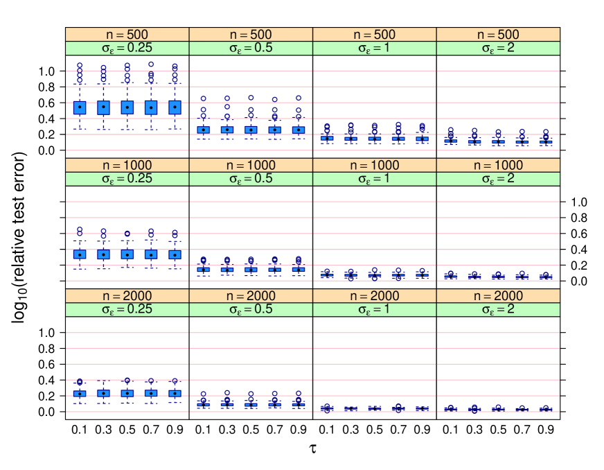
Figure S.1: Side-by-side boxplots of the logarithms, to base $10$, of relative test error for the Markov chain Monte Carlo Algorithm 2 for the simulation study described in the text. Each panel corresponds to a different combination of sample size and error standard deviation. Within each panel, the side-by-side boxplots compare relative test error as a function of the threshold parameter $\tau$.

S.3.1 Alternative Evaluation Metrics

The model selection recommendations of Section 3.5 are guided by the effect type misclassification rate since we believe this particular evaluation metric to be best aligned with the practical goal of achieving interpretable and parsimonious models. However effect type misclassification rate is just one of many possible evaluation metrics that could be used in simulation assessment, comparison and the guiding of tuning parameter choice. For example, the simulation studies of Hastie, Tibshirani & Tibshirani (2020), for a different regression-type setting, consider five evaluation metrics.

To see if and how our threshold parameter recommendations change if a different evaluation metric is used, we re-ran the Gaussian response simulation studies of Section 3.5 with effect type misclassification rate replaced by relative test error. For the situation where $d_{\circ}=0$ and $d_{\bullet}\in{\mathbb{N}}$, suppose that the selected model based on the data set $\boldsymbol{\mathscr{D}}$ corresponds to ${\widehat{f}}$ for some additive function ${\widehat{f}}:{\mathbb{R}}^{d_{\bullet}}\to{\mathbb{R}}$. If the true model corresponds to $f_{\mbox{\tiny true}}:{\mathbb{R}}^{d_{\bullet}}\to{\mathbb{R}}$ and the predictor $\boldsymbol{x}\in{\mathbb{R}}^{d_{\bullet}}$ is a random vector with density function $\mathfrak{p}(\boldsymbol{x})$ then the relative test error is

$$E\big{[}\big{\{}y-{\widehat{f}}(\boldsymbol{x})\}^{2}|\boldsymbol{\mathscr{D}}\big{]}\big{/}\sigma_{\varepsilon}^{2}\quad\mbox{where}\quad y\sim N\big{(}f_{\mbox{\tiny true}}(\boldsymbol{x}),\sigma_{\varepsilon}^{2}\big{)}.$$ (S.2)

Note that the expectation in (S.2) is over the predictor distribution corresponding to $\mathfrak{p}(\boldsymbol{x})$. The denominator in (S.2) is the Bayes error, corresponding to the situation where ${\widehat{f}}=f_{\mbox{\tiny true}}$. Therefore, (S.2) is the test error relative to the Bayes error and is an evaluation metric with a lower bound of $1$, and equals $1$ when $f_{\mbox{\tiny true}}$ is estimated perfectly.

Figures S.1 and S.2 are the analogues of Figures 3 and 4 with effect type misclassification rate replaced by relative test error. Monte Carlo approximations of the (S.2) numerator quantity based on 100,000 draws from the predictor distribution were used. To aid visualization the $\log_{10}$ transformation is applied to the relative test error values.

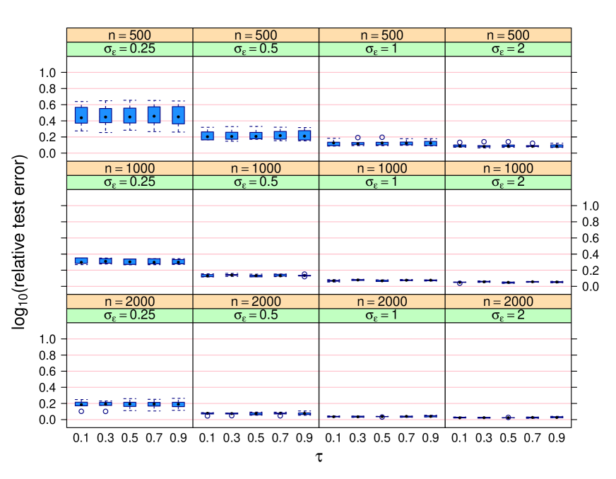
Figure S.2: Side-by-side boxplots of the logarithms, to base $10$, of relative test error for the mean field variational Bayes Algorithm 3 for the simulation study described in the text. Each panel corresponds to a different combination of sample size and error standard deviation. Within each panel, the side-by-side boxplots compare relative test error as a function of the threshold parameter $\tau$.

From Figures S.1 and S.2 we see that the relative test errors are lower for higher sample sizes, as expected. Somewhat counter-intuitively the relative test errors are lower for higher noise levels. However, comparisons of relative test error across different values of $\sigma_{\varepsilon}$ are not clear-cut when the estimators are subject to bias. In addition, relative test errors are barely affected by the choice of the thresholding parameter $\tau$. Lastly, the relative test errors based on mean field variational Bayes approximate inference are similar to those based on Markov chain Monte Carlo. It is interesting that this particular evaluation metric is not affected very much by the choices between Algorithms 2 and 3 and the value of the threshold parameter $\tau$.

S.3.2 Detailed Computing Time Results

We also conducted some more detailed involving computing times. One simulation study looked into the effect of sample size, whilst another one investigated how the number of candidate predictors impacts computing times. The results are presented in this section.

S.3.2.1 Assessment of the Effect of Sample Size

Our first detailed computing time simulation study was concerned with the effect of sample size. We fixed the candidate predictor dimensions to be $(d_{\circ},d_{\bullet})=(0,10)$ and let the sample size $n$ to range over the set

$$\{10^{k}:k=2,3,4,5,6\}.$$

The data were generated in a manner similar to that for the simulation studies described in Sections 3 and 4, with $100$ replications.

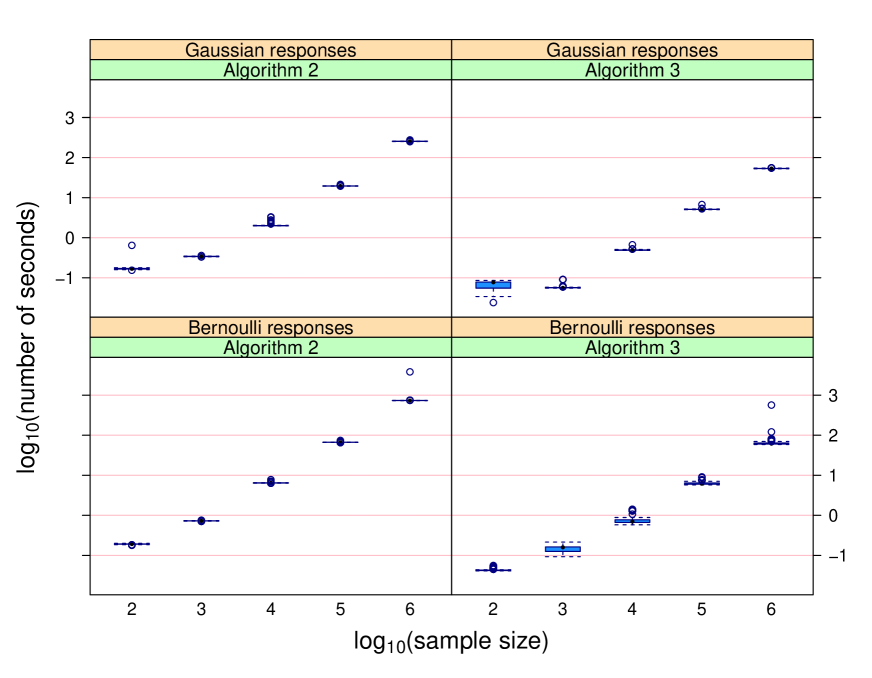
Figure S.3: Side-by-side box plots of computing time in seconds versus sample size for generalized additive model selection via Algorithms 2 and 3, for the first simulation study described in Section S.3.2. Each axis uses a $\log_{10}$ scale.

Figure S.3 summarizes the results using side-by-side boxplots of the logarithmically transformed computing times, broken down according to sample size, response type and whether or not Algorithm 2 or Algorithm 3 was used. The relationships between the mean logarithmic number of seconds and logarithmic sample size are approximately linear, which suggests a simple power law relationship between computing time and sample size. Simple linear regression analyses suggest that the power is close to $1$ and, hence, mean computing time is roughly proportional to sample size.

Figure S.3 also shows that use of Algorithm 3 leads to an approximately ten-fold reduction in computing time compared with Algorithm 2. For example, when $n=100,000$ the mean computing time of Algorithm 2 for Bernoulli responses is about $100$ seconds. For Algorithm 3 it is only about $10$ seconds.

S.3.2.2 Assessment of the Effect of the Number of Candidate Predictors

We also ran a simulation study concerned with the effect of the number of candidate predictors on computing time. The sample size was fixed at $5,000$ and $d_{\bullet}$, the number of candidate predictors that could enter the model non-linearly, varied over the set

$$\{2^{k}:k=1,2,3,4,5,6\}.$$

We generated the data in a manner similar to that for the simulation studies described in Sections 3 and 4 and, again, obtained $100$ replications.

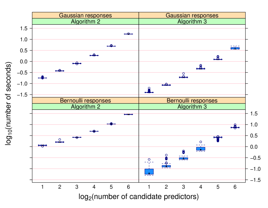
Figure S.4: Side-by-side box plots of computing time in seconds versus number of candidate predictors for generalized additive model selection via Algorithms 2 and 3, for the second simulation study described in Section S.3.2. The horizontal axis uses a $\log_{2}$ scale and the vertical axis uses a $\log_{10}$ scale.

Figure S.4 summarises the results in similar way to Figure S.3. Once again, there is approximate linearity within each panel with logarithmic scales. Simple linear regression analyses of the data within each panel of Figure S.4 suggest that the mean computing time is approximately proportional to $d_{\bullet}^{\kappa}$, with $\kappa$ dependent on the response distribution and fitting algorithm combination but within the interval $(1.2,1.5)$.

S.3.3 Hyperparameter Sensitivity Checks

Figure S.5 conveys the effect of the Half Cauchy distribution scale hyperparameters, denoted by $s_{\mbox{\tiny{$\beta$}}}$, $s_{\varepsilon}$ and $s_{u}$ in model (9), on the effect type misclassification rate. It is based on the simulation study set-up of Section 3.5 with the Markov chain Monte Carlo approach of Algorithm 2 and the threshold parameter $\tau$ set to our recommended default value of $0.5$. The scale hyperparameters ranged over the set

$$\{10^{k}:k=1,2,3,4\}.$$

Figure S.5 indicates that our default version of Algorithm 2 is not sensitive to the Half Cauchy distribution scale hyperparameter values.

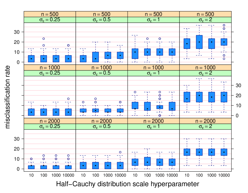
Figure S.5: Side-by-side boxplots of misclassification rate for varying values of the Half Cauchy distribution scale hyperparameter for the Gaussian response version of Algorithm 2, for the first simulation study described in Section S.3.3.

Figure S.6 is similar to Figure S.5, but is for the mean field variational Bayes approach used by Algorithm 3 with $\tau$ set to the default value of $0.1$. Once again, low sensitivity to the Half Cauchy distribution scale hyperparameter values is exhibited.

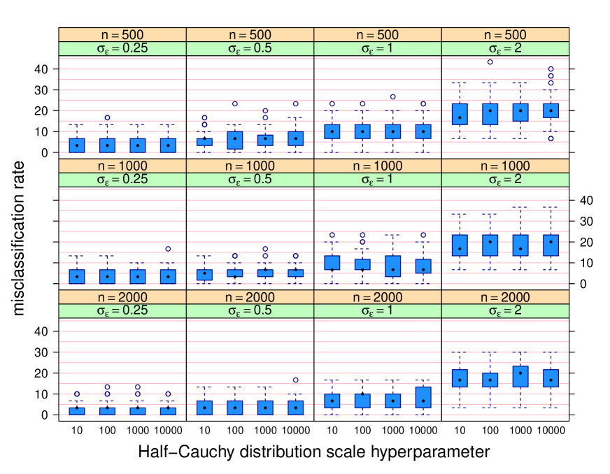
Figure S.6: Side-by-side boxplots of misclassification rate for varying values of the Half Cauchy distribution scale hyperparameter for the Gaussian response version of Algorithm 3, for the first simulation study described in Section S.3.3.

Reference

Hastie, T., Tibshirani, R. & Tibshirani, R. (2020). Best subset, forward stepwise of lasso? Analysis and recommendations based on extensive comparisons. Statistical Science,35, 579–592.