A General Framework for Evaluating Robustness of Combinatorial Optimization Solvers on Graphs

Abstract

Solving combinatorial optimization (CO) on graphs is among the fundamental tasks for upper-stream applications in data mining, machine learning and operations research. Despite the inherent NP-hard challenge for CO, heuristics, branch-and-bound, learning-based solvers are developed to tackle CO problems as accurately as possible given limited time budgets. However, a practical metric for the sensitivity of CO solvers remains largely unexplored. Existing theoretical metrics require the optimal solution which is infeasible, and the gradient-based adversarial attack metric from deep learning is not compatible with non-learning solvers that are usually non-differentiable. In this paper, we develop the first practically feasible robustness metric for general combinatorial optimization solvers. We develop a no worse optimal cost guarantee thus do not require optimal solutions, and we tackle the non-differentiable challenge by resorting to black-box adversarial attack methods. Extensive experiments are conducted on 14 unique combinations of solvers and CO problems, and we demonstrate that the performance of state-of-the-art solvers like Gurobi can degenerate by over 20% under the given time limit bound on the hard instances discovered by our robustness metric, raising concerns about the robustness of combinatorial optimization solvers.

1 Introduction

The combinatorial optimization (CO) problems on graphs are widely studied due to their important applications including aligning cross-modality labels [21], discovering vital seed users in social networks [43], tackling large-scale knapsack problems [41] and scheduling jobs [23] in data centers, etc. However, CO problems are non-trivial to solve due to the NP-hard challenge, whereby the optimal solution can be nearly infeasible to achieve for even medium-sized problems. Existing approaches to practically tackle CO include heuristic methods [33, 38], powerful branch-and-bound solvers [12, 32, 8] and recently developed learning-based models [18, 23, 20].

Despite the success of solvers in various combinatorial tasks, little attention has been paid to the vulnerability and robustness of combinatorial solvers. Within the scope of the solvers and problems studied in this paper, our study shows that the performance of the solver may degenerate a lot given certain data distributions that should lead to the same or better solutions compared to the original distribution assuming the solver works robustly. We also validate in experiments that such a performance degradation is neither caused by the inherent discrete nature of CO. Such a discovery raises our concerns about the stability and robustness of combinatorial solvers, which is also aware by [34, 9]. However, [34] focuses on theoretical analysis and requires the optimal solution, which is infeasible to reach in practice. [9] applies the attack-and-defense study in deep learning into learning-based combinatorial optimization models, requiring a differentiable neural network that is infeasible for general solvers that can often be undifferentiable. Our paper also differs from the namely “robust optimization” [2], where the expected objective score is optimized given known data distribution. We summarize the challenges and our initiatives of evaluating the robustness of existing solvers as follows:

1) Robustness metric without optimal solutions: The underlying NP-hard challenge of combinatorial optimization prohibits us from obtaining the optimal solutions. However, the robustness metric proposed by [34] requires optimal solutions, making this metric infeasible in practice. In this paper, we propose a problem modification based robustness evaluation method, whereby the solvers’ performances are evaluated on problems that can guarantee no worse optimal costs compared to the original problem, without requiring the optimal solutions.

2) Robustness metric of general (non-differentiable) solvers: Despite the recently developed deep-learning solvers, most existing solvers are non-differentiable due to the discrete combinatorial nature. Thus, the gradient-based robustness metric by [9] has the limitation to generalize to general solvers. In this paper, we develop a reinforcement learning (RL) based attacker by regarding arbitrary types of solvers as black-boxes, and the RL agent is trained by policy gradient without requiring the solver to be differentiable. Our framework also owns the flexibility where the agent can be replaced by other search schemes e.g. simulated annealing.

Table 1: Comparing our framework (ROCO) with FGSM [10] and RL-S2V [6]. $\epsilon$-perturb means the change of one pixel should be bounded in $\epsilon$. B-hop neighbourhood means the new attack edges can only connect two nodes with distance less than $B$.

Method	Data	Task	Attack target	Attack budget	Attack principle
FGSM [10]	image	classification	pixels	$\epsilon$-Perturb	invisible change
RL-S2V [6]	graph	classification	edges (connectivity)	# edge	B-hop neighbour
ROCO (ours)	CO instance	CO solution	edges (constraints/cost)	# edge	no worse optimum

Being aware that many CO problems can be essentially formulated as a graph problem and there are well-developed graph-based learning models [29, 19, 35], the scope of this paper is restricted within combinatorial problems on graphs following [18, 37]. To develop a problem modification method that achieves no worse optimal costs, we propose to modify the graph structure with a problem-dependent strategy exploiting the underlying problem natures. Two types of strategies are developed concerning the studied four combinatorial problems: 1) loosening the constraints such that the feasible space can be enlarged while the original optimal solution is preserved; 2) lowering the cost of a partial problem such that the objective value of the original optimal solution can become better. Such strategies are feasible when certain modifications are performed on the edges of the input graph, and tackle the challenge that we have no access to the optimal solutions. It is also ensured that the generated data distributes closely to the original data by restricting the number of edges modified. The graph modification steps are performed by our proposed attackers that generate problem instances where the solvers’ performances degenerate, and we ensure the no worse optimal costs guarantee by restricting the action space of the attackers.

Our framework can be seen as the attack on the solvers and how much the worst cases near the clean instances will do harm to the solver are considered as the robustness. Tab. 1 compares our framework to classical works on adversarial attacks for images and graphs. The main contributions of this paper are summarized as follows:

1) We propose Robust Combnaotorial Optimization (ROCO), the first general framework (as shown in Fig. 1) to evaluate the robustness of combinatorial solvers on graphs without requiring optimal value or differentiable property.

2) We design a novel robustness evaluation method with no worse optimal costs guarantee to eliminate the urgent requirements for the optimal solution of NP-hard CO problems. We develop a reinforcement learning (RL) based attacker combined with other search-based attackers to regard the solvers as black-boxes, making the non-differentiable ones available.

3) Case studies are conducted on four common combinatorial tasks: Directed Acyclic Graph Scheduling, Asymmetric Traveling Salesman Problem, Maximum Coverage, and Maximum Coverage with Separate Coverage Constraint, with three kinds of solvers: traditional solvers, learning-based solver and specific MILP solver like Gurobi. Code will be made publicly available.

4) The results raise potential concerns about the robustness, such as the $20\%$ performance decrease for the commercial solver Gurobi. They also help verify the existing theory about data generation [39] and provide ideas (e.g. adversarial training and parameter tuning) to develop more robust solvers.

2 Related Works

Combinatorial optimization solvers. As a long-standing area, there exist many traditional CO algorithms, including but not limited to greedy algorithms, heuristic algorithms like simulated annealing (SA) [33], Lin–Kernighan–Helsgaun (LKH3) [14], and branch-and-bound solvers like CBC [8], SCIP [32], and Gurobi [12]. Besides, driven by the recent development of deep learning and reinforcement learning, many learning-based methods have also been proposed to tackle these problems. A mainstream approach using deep learning is to predict the solution end-to-end, such as the supervised model Pointer Networks [36], reinforcement learning models S2V-DQN [18] and MatNet [20]. Though these methods did perform well on different types of CO problems, they are not that robust and universal, as discussed in [1], the solvers may get stuck around poor solutions in many cases. The sensitivity of CO algorithms is theoretically characterized in [34], however the metric in [34] requires optimal solutions which are usually unavailable in practice concerning the NP-hard challenge in CO.

Adversarial attack for neural networks. Since the seminal study [31] shows that small input perturbations can change model predictions, many adversarial attack methods have been devised to construct such attacks. In general, adversarial attacks can be roughly divided into two categories: white-box attacks with access to the model gradients, e.g. [10, 22, 3], and black-box attacks, with only access to the model predictions, e.g. [16, 25]. Besides image and text adversarial attacks [17], given the importance of graph-related applications and the successful applications of graph neural networks (GNN) [29], more attention is recently paid to the robustness of GNNs [6]. Besides, the recent adversarial graph matching (GM) network shows how to fulfill attack or defense via perturbing or regularizing geometry property on the GM solver. [42] degrades the quality of GM by perturbing nodes to more dense regions while [27] improves robustness by separating nodes to be distributed more broadly. However, the techniques are deliberately tailored to the specific problem and can hardly generalize to the general CO problems. [9] develops a gradient-based attack method for CO learning models that must be differentiable, and cannot generalize to solvers that are usually non-differentiable due to the discrete nature. The black-box differentiation technique [26] is restricted for linear objective. We aim to propose a general pipeline by developing more flexible black-box attacks.

3 ROCO Framework

3.1 Adversarial Robustness for CO

CO problem. In general, a CO problem aims to find the optimal solution under a set of constraints (usually encoded by a latent graph). Typically, we formulate a CO problem $Q$ as:

$$\min_{\mathbf{x}}c(\mathbf{x},Q)\ \ s.t.\ \ h_{i}(\mathbf{x},Q)\leq 0,\ i=1,...,I$$ (1)

where $\mathbf{x}$ denotes the decision variable (i.e. solution) that should be discrete, $c(\mathbf{x},Q)$ denotes the cost function given problem instance $Q$ and $\{h_{i}(\mathbf{x},Q)\}_{i=1}^{I}$ represents the set of constraints. For example, in DAG scheduling, the constraints ensure that the solution $\mathbf{x}$, i.e. the execution order of the DAG job nodes, lies in the feasible space and does not conflict the topological dependency structure of $Q$. However, due to the NP-hard nature, the optimal solution $\mathbf{x}^{*}$ can be intractable within polynomial time. Therefore, we use a solver $\hat{\mathbf{x}}=f_{\theta}(Q)$, which gives a mapping $f_{\theta}:\mathbb{Q}\rightarrow\mathbb{X}$ to approximate the optimal solution $\mathbf{x}^{*}$. In this work, $\theta$ are solvers’ parameters (e.g. weights and biases in a neural solver, hyperparameters in Gurobi), $Q\in\mathbb{Q}$ is the problem instance, and $\hat{\mathbf{x}}\in\mathbb{X}$ is the approximated solution. $\hat{\mathbf{x}}$ also lies in the feasible space that satisfies all the constraints.

Solvers’ robustness. In this paper, we would like to raise the concern that the estimation capability of the solvers can be unstable and fail on certain hard instances. Thus, we need methods to discover the non-trivial hard instances for the solvers as the robustness metric. Here non-trivial means these hard instances are not obtained by trivial operations like increasing the size of problems. In short, given a certain solver $f_{\theta}$, we design an attacker (i.e. perturbation model) $g$ to discover hard instances around existing clean instances $\tilde{Q}=g(f_{\theta},Q)$. For example, the attacker can modify the limited number of constraints in $Q$ to get a new problem $\tilde{Q}$. Besides working as a robustness metric, the discovered hard instances can guide the parameter setting of solvers, i.e. design solvers’ parameters $\theta$ for better performance (robustness) on hard instances, but it may be beyond the scope of this paper and we mainly focus on developing the first practically feasible robustness metric.

Robustness metric. A natural evaluation of the solvers’ robustness is to use the gap $c(\hat{\mathbf{x}},Q)-c(\mathbf{x}^{*},Q)$ [34], where a narrower gap stands for a better performance. However, the optimum $\mathbf{x}^{*}$ is usually unavailable due to the NP-hardness. In this paper, we propose a robustness evaluation method, and the attack is defined by:

Definition 1 (Successful Attack).

Given a certain solver $f_{\theta}$ and a clean CO problem instance $Q$, we obtain a new problem $\tilde{Q}=g(f_{\theta},Q)$ by the attacker $g$ s.t. the optimal cost value after perturbation will become no-worse, i.e. $c(\mathbf{\tilde{x}}^{*},\tilde{Q})\leq c(\mathbf{x}^{*},Q)$. A successful attack occurs when $c(f_{\theta}(\tilde{Q}),\tilde{Q})>c(f_{\theta}(Q),Q)$.

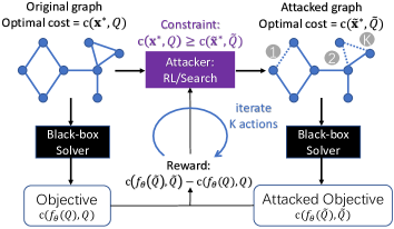
(a) ROCO framework

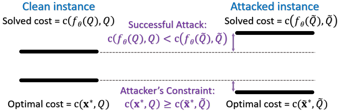
(b) Successful attack

Figure 1: Overview and intuition of our attack framework. Left: Overview of our attack framework ROCO for CO solvers. ROCO targets on the CO problems which can be encoded by graph (often holds in practice). Here modifying the edges in the encoded graph represents modifying constraints or lowering the cost in CO. Right: The definition of a successful attack.

The intuition is that we restrict the attacker to discover a new problem instance with no-worse optimal cost value, such that the gap between the solver and the optimal will be definitely enlarged if the solver gives a worse cost value:

$$c(\mathbf{\tilde{x}}^{*},\tilde{Q})\leq c(\mathbf{x}^{*},Q),\ c(f_{\theta}(\tilde{Q}),\tilde{Q})>c(f_{\theta}(Q),Q)\Rightarrow$$ (2)

$$c(f_{\theta}(Q),Q)-c(\mathbf{x}^{*},Q)<c(f_{\theta}(\tilde{Q}),\tilde{Q})-c(\mathbf{\tilde{x}}^{*},\tilde{Q}),$$

which represents a successful attack (see Fig. 1(b)).

Attacker’s target. In conclusion, the attacker should maximize the solver’s cost value after perturbation while conforming to the no-worse restriction. Therefore, we formulate our attack objective:

$$\max_{\tilde{Q}}\quad c(f_{\theta}(\tilde{Q}),\tilde{Q})-c(f_{\theta}(Q),Q)$$ (3)

$$s.t.\quad\tilde{Q}=g(f_{\theta},Q),\ c(\mathbf{\tilde{x}}^{*},\tilde{Q})\leq c(\mathbf{x}^{*},Q)$$

Attacker’s constraints. Two types of strategies are developed to meet the no worse optimal cost constraint for the attackers: 1) Loosening the constraints of the problem. In this way, the original optimal solution still lies in the feasible space and its cost is not affected, while the enlarged feasible space may include better solutions. Therefore, the new optimal cost cannot be worse than the original one, and we discover this strategy effective for DAG scheduling (see Section 4.1). 2) Modifying a partial problem by lowering the costs. Such a strategy ensures that the cost that corresponds to the original optimal solution can never become worse, and there are also chances to introduce solutions with lower costs. We demonstrate its successful application in traveling salesman (see Section 4.2) and max coverage problems (see Section 4.3 & Appendix B).

Attack via graph modification. As we have mentioned above, a CO problem $Q$ can usually be encoded by a latent graph $\mathcal{G}=(V,E)$. For example, the DAG problem can be represented by a directed acyclic graph (see Fig. 2), s.t. the graph nodes stand for the DAG jobs, the directed edges denote the sequential constraints for the jobs, and the node features represent the jobs’ completion time. Hence, the perturbation to the problem instance can be conducted by modifications to the graph structure [6]. Besides, to get non-trivial hard instances around clean examples, the attack is limited within a given attack budget $K$, e.g. the attacker can remove $\leq K$ edges in a DAG problem $Q$. Typically, in our setting, the graph modification is all conducted by modifying edges in the graph.

3.2 Implementations of the Attacker

Random attack baseline. The baseline simply chooses and modifies $K$ random edges sequentially, then calculates the new solution cost. The baseline is designed to reflect the instability of CO problems, we compare other attackers (which achieve much higher attack effects) to the random attack baseline to claim that our framework can uncover far more hard instances than the inherent instability caused by the CO problems.

Reinforcement learning attacker (ROCO-RL). We use Eq. 3 as the objective and resort to reinforcement learning (RL) to find $\tilde{Q}$ in a data-driven manner. Specifically, we modify the graph structure and compute $c(f_{\theta}(\tilde{Q}),\tilde{Q})$ alternatively, getting rewards that will be fed into the PPO [30] framework and train the agent.

Given an instance ($f_{\theta},Q$) along with a modification budget $K$, we model the attack via sequential edge modification as a Markov Decision Process (MDP):

State. The current problem instance $Q^{k}$ (i.e. the problem instance $\tilde{Q}$ obtained after $k$ actions) is treated as the state. The original problem instance $Q^{0}=Q$ is the starting state.

Action. The attacker is allowed to modify edges in the graph. So a single action at time step $k$ is $a^{k}\in\mathcal{A}^{k}\subseteq E^{k}$. Here our action space $\mathcal{A}^{k}$ is usually a subset of all the edges $E^{k}$ since we can narrow the action space (i.e. abandon some useless edge candidates) according to the previous solution $f_{\theta}(Q^{k})$ to speed up our algorithm. Furthermore, we decompose the action space ($O(|V|^{2})\rightarrow O(|V|)$) by transforming the edge selection into two sequential node selections: first selecting the start node, then the end node.

Reward. The objective of the new CO problem $Q^{k+1}$ is $c(f_{\theta}(Q^{k+1}),Q^{k+1})$. To maximize the new cost value, we define the reward as the increase of the objective:

$$r=c(f_{\theta}(Q^{k+1}),Q^{k+1})-c(f_{\theta}(Q^{k}),Q^{k})$$ (4)

Terminal. Once the agent modifies $K$ edges or edge candidates become empty, the process stops.

The input and constraints of a CO problem can often be encoded in a graph $\mathcal{G}=(V,E)$, and the PPO agent (i.e. the actor and the critic) should behave according to the graph features. We resort to the Graph Neural Networks (GNNs) for graph embedding:

$$\textbf{n}=\mbox{GNN}(\mathcal{G}^{k}),\ \textbf{g}=\mbox{AttPool}(\textbf{n})$$ (5)

where $\mathcal{G}^{k}$ is the corresponding graph of problem $Q^{k}$, the matrix n (with the size of node number $\times$ embedding dim) is the node embedding. An attention pooling is used to extract a graph level embedding g. The GNN model can differ by the CO problems (details in Appendix C). After graph feature extraction, we design the actor and critic nets:

Critic. The critic predicts the value of each state $Q^{k}$. Since it aims at reward maximization, a max-pooling layer is adopted over all node features which are concatenated (denoted by $[\cdot||\cdot]$) with the graph embedding $\mathbf{g}$, fed into a network (e.g. ResNet block [13]) for value prediction:

$$\mathcal{V}(Q^{k})=\mbox{ResNet}_{1}([\mbox{MaxPool}(\textbf{n})||\textbf{g}])$$ (6)

Actor. The edge selection is implemented by selecting the start and end node sequentially. The action scores are computed using two independent ResNet blocks, and a Softmax layer is added to regularize the scores into probability $[0,1]$:

$$P(a_{1}) =\mbox{Softmax}(\mbox{ResNet}_{2}([\textbf{n}||\textbf{g}])),$$ (7)

$$P(a_{2}|a_{1}) =\mbox{Softmax}(\mbox{ResNet}_{3}([\textbf{n}||\textbf{n}[a_{1}]||\textbf{g}))$$

where $\textbf{n}[a_{1}]$ denotes node $a_{1}$’s embedding. We add the feature vector of the selected start node for the end node selection. For training, actions are sampled w.r.t. their probabilities. For testing, beam search is used to find the optimal solution: actions with top-$B$ probabilities are chosen for each graph in the last time step, and only those actions with top-$B$ rewards will be reserved for the next search step (see Alg. 1).

Input: Input problem $Q$; solver $f_{\theta}$; max number of actions $K$; beam size $B$.

$Q^{0}_{1..B}\leftarrow Q$; $\tilde{Q}\leftarrow Q$; # set initial state

for $k\leftarrow 1..K$ do

       for $b\leftarrow 1..B$ do

             # do beam search for problems in last step

             Predict $P(a_{1})$, $P(a_{2}|a_{1})$ on $Q^{k-1}_{b}$;

             Select $(a_{1},a_{2})$ with top-$B$ probabilities;

      for each $(b,a_{1},a_{2})$ pair do

             $Q^{\prime}(b,a_{1},a_{2})\leftarrow$ modify edge $(a_{1},a_{2})$ in $Q^{k-1}_{b}$;

             if $c(f_{\theta},Q^{\prime}(b,a_{1},a_{2}))>c(f_{\theta},Q^{*})$ then

                   $\tilde{Q}\leftarrow Q^{\prime}(b,a_{1},a_{2})$

                   # update the best attacked problem

            

      Sort $Q^{\prime}(\cdot,\cdot,\cdot)$ w.r.t. cost values by decreasing order;

       $Q^{k}_{1..B}\leftarrow Q^{\prime}_{1..B}$; # select top-$B$ problems for the next step

Output: Best attacked problem instance $\tilde{Q}$.

Algorithm 1 Attack by iterative edge manipulation

Other attacker implementations. We also implement three other traditional attack algorithms for comparison: random search, optimum-guided search and simulated annealing.

i) Random Search (ROCO-RA): In each iteration, an edge is randomly chosen to be modified in the graph and it will be repeated for $K$ iterations. Different from the random attack baseline without any search process, we will run $N$ attack trials and choose the best solution. Despite its simplicity, it can reflect the robustness of solvers with the cost of time complexity $O(NK)$.

ii) Optimum-Guided Search (ROCO-OG): This method focuses on finding the optimum solution during each iteration. We use beam search to maintain the best $B$ current states and randomly sample $M$ different actions from the candidates to generate next states. The number of iterations is set to be no more than $K$, so its time complexity is $O(BMK)$.

iii) Simulated Annealing (ROCO-SA): Simulated annealing [33] comes from the idea of annealing and cooling used in physics for particle crystallization. In our scenario, a higher temperature indicates a higher probability of accepting a worse solution, allowing to jump out of the local optimum. As the action number increases, the temperature will decrease, and we are tending to reject the bad solution. The detailed process is shown in Appendix A and we will repeat the algorithm for $N$ times. SA is a fine-tuned algorithm and we can use grid search to find the best parameter to fit the training set. Its time complexity is $O(NMK)$.

Tab. 7 in Appendix H concludes the attack methods property and time complexity. Since these three traditional algorithms are inherently stochastic, we run them multiple times to calculate the mean and standard deviation. Meanwhile, the reinforcement learning attacker is deterministic because we always use the best trained model to modify graph structures on the testing set.

4 Studied CO Tasks and Results

We conduct experiments on four representative CO tasks: Directed Acyclic Graph Scheduling, Asymmetric Traveling Salesman Problem, Maximum Coverage and Maximum Coverage with Separate Coverage Constraint. Considering the page limitation, the details of the last task is postponed to Appendix B. We also test the robustness of representative solvers including heuristics [14, 11], branch-and-bound solvers [8, 32, 12] and learning-based methods [20]. The detailed graph embedding methods for the four tasks is shown in Appendix C. In Appendix H, we provide training and evaluation hyperparameters of different solvers for fair time comparison and reproducibility. Experiments are run on our heterogeneous cluster with RTX 2080Ti and RTX 3090.

4.1 Task I: Directed Acyclic Graph Scheduling

Task scheduling for heterogeneous systems and various jobs is a practical problem. Many systems formulate the job stages and their dependencies as a Directed Acyclic Graph (DAG) [28, 4, 40], as shown in Fig. 2. The data center has limited computing resources to allocate the jobs with different resource requirements. These jobs can run in parallel if all their parent jobs have finished and the required resources are available. Our goal is to minimize the makespan (i.e. finish all jobs ASAP.)

Table 2: Evaluation of solvers for DAG scheduling. Clean makespans are reported on the clean test set. Larger attacked makespans mean stronger attacker. Random denotes the random attack baseline with the mean and std tested for 100 trials. ROCO-RA/OG/SA are tested for 10 trials to calculate the mean and std. ROCO-RL is reported with a single value since it is invariant to different random seeds. All four attack methods perform better than the random attack baseline, which usually leads to a shorter makespan (unsuccessful attack), proving that our attack framework can find more hard instances than those because of the inherent instability of CO problems. Tetris is the most robust solver on dataset sizes of 50 and 150 while Critical path is more robust on size 100.

Solver	Problem Size:	Clean Makespan	Attack Method (Attacked Makespans $(\times 10^{5})$)
	#job	$(\times 10^{5})\downarrow$	Random	ROCO-RA	ROCO-OG	ROCO-SA	ROCO-RL
Shortest Job First	50	1.0461	$1.0406\pm 0.0035$	$1.0574\pm 0.0013$	$1.0600\pm 0.0019$	$\textbf{1.0622}\pm\textbf{0.0007}$	$1.0608$
Critical Path	50	0.8695	$0.8828\pm 0.0077$	$0.9402\pm 0.0038$	$0.9480\pm 0.0021$	$\textbf{0.9528}\pm\textbf{0.0013}$	$0.9500$
Tetris [11]	50	0.8227	$0.8582\pm 0.0079$	$0.0952\pm 0.0049$	$0.9218\pm 0.0066$	$0.9380\pm 0.1153$	0.9397
Shortest Job First	100	1.9160	$1.8832\pm 0.0075$	$1.9210\pm 0.0006$	$1.9239\pm 0.0008$	$1.9239\pm 0.0008$	1.9263
Critical Path	100	1.6018	$1.6279\pm 0.0167$	$1.7391\pm 0.0045$	$1.7456\pm 0.0043$	$1.7480\pm 0.0003$	1.7498
Tetris [11]	100	1.5186	$1.5830\pm 0.0196$	$1.7201\pm 0.0055$	$1.7099\pm 0.0111$	$1.7418\pm 0.0074$	1.7526
Shortest Job First	150	2.8578	$2.8281\pm 0.0074$	$2.8818\pm 0.0020$	$2.8898\pm 0.0023$	$2.8950\pm 0.0014$	2.8964
Critical Path	150	2.4398	$2.4254\pm 0.0203$	$2.5698\pm 0.0093$	$2.5928\pm 0.0090$	$2.6020\pm 0.0029$	2.6069
Tetris [11]	150	2.2469	$2.3581\pm 0.0270$	$2.4988\pm 0.0191$	$2.5039\pm 0.0202$	$\textbf{2.5399}\pm\textbf{0.0058}$	$2.5329$

Solvers. We choose three popular heuristic solvers as our attack targets. First, the Shortest Job First algorithm chooses the jobs greedily with minimum completion time. Second, the Critical Path algorithm finds the bottlenecks and finishes the jobs in the critical path sequence. Third, the Tetris [11] scheduling algorithm models the jobs as 2-dimension blocks in the Tetris games according to their finishing time and resource requirement.

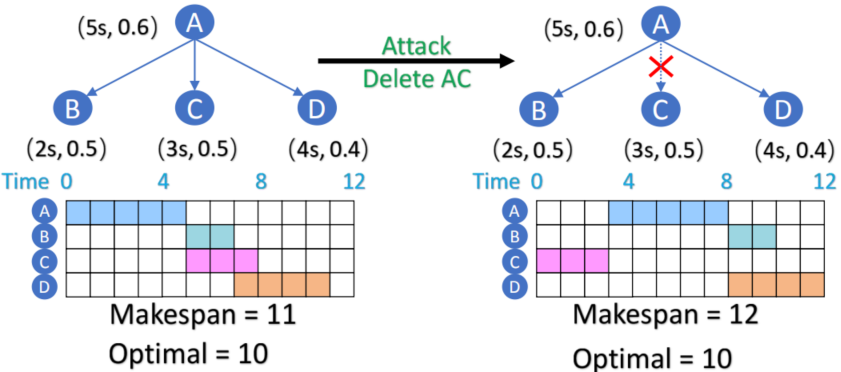
Figure 2: DAG attack on Shortest Job First algorithm. The edges show sequential dependencies. The $(x,y)$ tuple of each node means running time ($x$) and resource occupancy rate ($y$).

Attack model. The edges in a DAG represent job dependencies, and removing edges will relax the constraints. After removing existing edges in a DAG, it is obvious that the new solution will be equal to or better than the original one since there are fewer restrictions. As a result, in the DAG scheduling tasks, the attack model is to selectively remove existing edges.

Dataset. We use TPC-H dataset (http://tpc.org/tpch/default5.asp), composed of business-oriented queries and concurrent data modification. Many DAGs referring to computation jobs, have tens or hundreds of stages with different duration and numbers of parallel tasks. We gather the DAGs randomly and generate three different sizes of datasets, TPC-H-50, TPC-H-100, TPC-H-150, each with $50$ training and $10$ testing samples. The DAG nodes have two properties: execution time and resource requirement.

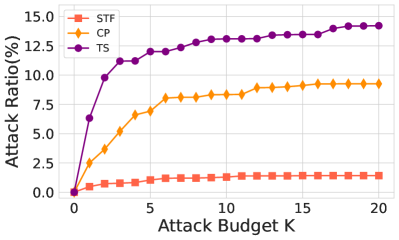
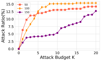
Figure 3: Left: RL Attack results w.r.t. attack budgets $K$ on TPC-H-50 dataset for solvers Shortest Job First(SJF), Critical Path(CP) and Tetris(TS). Ratio represents the increase of makespan after attack w.r.t. clean makespans. Right: RL Attack results w.r.t. attack budgets $K$ on TPC-H-50/100/150 datasets for the Tetris (TS) solver.

Results and analysis. Tab. 2 reports the results of our four attack methods. In the designed attack methods, RL outperforms other learning-free methods in most cases, illustrating the correctness of our feature extraction techniques and training framework. It is worth noting that even the simplest random search (ROCO-RA) can cause a significant performance degradation to the CO solvers, showing their vulnerability and the effectiveness of the attack framework. Fig. 3 (left) shows the attack ratio for different solvers on TPC-H-50. In general, the attack ratio increases then flattens out w.r.t. attack budgets, corresponding with the fact that we can find more hard instances under a larger searching space (but harder to find new successfully attacked instances as we remove more constraints). Fig. 3 (right) demonstrates the effect of attack budgets on different sizes of datasets using the same solver Tetris. The figure illustrates that attack ratios on smaller datasets tend to flatten first (larger datasets allow for more attack actions), which can guide us to select the right number of attack actions for different datasets.

4.2 Task II: Asymmetric Traveling Salesman

The classic traveling salesman problem (TSP) is to find the shortest cycle to travel across all the cities. Here we tackle the extended version namely asymmetric TSP (ATSP) for its generality.

Solvers. The robustness of four algorithms are evaluated: First, Nearest Neighbour greedily adds the nearest city to the tour. Second, Furthest Insertion finds the city with the furthest distance to the existing cities in the tour and inserts it. Third, Lin-Kernighan Heuristic (LKH3) [14] is the traditional SOTA TSP solver. Finally, Matrix Encoding Networks (MatNet) [20] claims as a SOTA learning-based solver for ATSP and flexible flow shop (FFSP).

Attack model. The attack is to choose an edge and half its value, after which we will get a no-worse theoretical optimum since the length of any path will maintain the same or even decrease. To reduce the action space, we will not select the edges in the current path predicted by the solver at the last time step. A successful attack example is shown in Fig. 5 in Appendix D.

Table 3: Evaluation of solvers for ATSP. A Larger tour length means a stronger attacker. Random denotes the random attack baseline with the mean and std tested for 100 trials. ROCO-RA/OG/SA are tested for 10 trials to calculate the mean and std. ROCO-RL is reported with a single value since it is invariant to different random seeds. MatNet (fixed) represents training MatNet with 10000 fixed ATSP instances. LKH3 and MatNet are more robust than peer solvers.

Solver	Problem	Clean Tour	Attack Method (Attacked Tour Length $Length(\times 10^{6})$)
	Size: # city	$(\times 10^{6})\downarrow$	Random	ROCO-RA	ROCO-OG	ROCO-SA	ROCO-RL
Nearest Neighbour	20	1.9354	$1.9143\pm 0.0259$	$2.1307\pm 0.0153$	$2.1162\pm 0.0323$	$2.1344\pm 0.0159$	2.1858
Furthest Insertion	20	1.6092	$1.5847\pm 0.0142$	$1.6953\pm 0.0105$	$1.6926\pm 0.0117$	$1.7183\pm 0.0114$	1.7469
LKH3 [14]	20	1.4595	$1.4201\pm 0.0089$	$1.4599\pm 0.0003$	$1.4599\pm 0.0004$	$1.4610\pm 0.0017$	1.4611
MatNet [20]	20	1.4616	$1.4237\pm 0.0089$	$1.4674\pm 0.0012$	$1.4683\pm 0.0006$	$1.4683\pm 0.0009$	1.4708
MatNet (fixed) [20]	20	1.4623	$1.4227\pm 0.0086$	$1.4665\pm 0.0013$	$1.4687\pm 0.0004$	$1.4714\pm 0.0013$	1.4737
Nearest Neighbour	50	2.2247	$2.2221\pm 0.0131$	$2.3635\pm 0.0082$	$2.3809\pm 0.0096$	$2.4058\pm 0.0151$	2.4530
Furthest Insertion	50	1.9772	$1.9730\pm 0.0091$	$2.0593\pm 0.0071$	$2.0466\pm 0.0125$	$2.0632\pm 0.0089$	2.1150
LKH3 [14]	50	1.6621	$1.6493\pm 0.0042$	$1.6653\pm 0.0007$	$1.6656\pm 0.0007$	$\textbf{1.6682}\pm\textbf{0.0010}$	$1.6679$
MatNet [20]	50	1.6915	$1.6786\pm 0.0051$	$1.7153\pm 0.0012$	$1.7204\pm 0.0016$	$1.7255\pm 0.0012$	1.7279
MatNet(fixed) [20]	50	1.6972	$1.6894\pm 0.0054$	$1.7171\pm 0.0021$	$1.7205\pm 0.0005$	$1.7279\pm 0.0007$	1.7349
Nearest Neighbour	100	2.1456	$2.1423\pm 0.0079$	$2.2319\pm 0.0099$	$2.2213\pm 0.0152$	$2.2273\pm 0.0112$	2.2533
Furthest Insertion	100	1.9209	$1.9188\pm 0.0061$	$1.9762\pm 0.0088$	$1.9782\pm 0.0111$	$1.9853\pm 0.0063$	2.0144
LKH3 [14]	100	1.5763	$1.5716\pm 0.0016$	$1.5826\pm 0.0006$	$1.5848\pm 0.0005$	$1.5856\pm 0.0003$	1.5862
MatNet [20]	100	1.6545	$1.6492\pm 0.0036$	$1.6772\pm 0.0012$	$1.6815\pm 0.0005$	$1.6841\pm 0.0007$	1.6873
MatNet (fixed) [20]	100	1.6556	$1.6498\pm 0.0037$	$1.6788\pm 0.0008$	$1.6823\pm 0.0003$	$1.6846\pm 0.0015$	1.6919

Dataset. The dataset comes from [20], consisting of ‘tmat’ class ATSP instances which have the triangle inequality and are widely studied by the operation research community [5]. We solve the ATSP of three sizes, $20$, $50$ and $100$ cities. The distance matrix is fully connected and asymmetric, and each dataset consists of $50$ training samples and $20$ testing samples.

Results and analysis. Tab. 3 reports the attack results of four target solvers. where the RL based attack outperforms other methods in most cases. We can also conclude that LKH3 is the most robust among all compared solvers, possibly because its local search nature can jump out of local optimums. MatNet generates different random problem instances for training in each iteration. The comparison between “MatNet” and “MatNet (fixed)” proves that the huge amount of i.i.d. training instances promotes both the performance and the robustness of the model. As [39] points out, learning-based solvers for CO cannot be trained sufficiently due to the theoretical limitation of data generation. Thus, the training paradigm with large unlabeled data can be a good choice for learning-based CO solvers.

4.3 Task III: Maximum Coverage

The maximum coverage (MC) problem is a classical problem that is widely studied in approximation algorithms. Specifically, as input we will be given several sets $\mathcal{S}=\{S_{1},S_{2},...,S_{m}\}$ and a number $k$. The sets consist of weighted elements $e\in\mathcal{E}$ and may have overlap with each other. Our goal is to select at most $k$ of these sets such that the maximum weight of elements are covered. Formally, the above problem can be formulated as follows:

$$\max_{\mathcal{S}^{\prime}}\sum_{e\in\mathcal{E}}w(e)\times\mathbb{I}(e\in\bigcup_{S_{i}\in\mathcal{S}^{\prime}}S_{i})\quad s.t.\quad\mathcal{S}^{\prime}\subseteq\mathcal{S},\ |\mathcal{S}^{\prime}|\leq k$$ (8)

where $w(\cdot):\mathcal{E}\rightarrow\mathbb{R}$ denotes the weight of a certain element.

Table 4: Evaluation of solvers for MC. The time limit is shown in brackets for branch-and-bound solvers, which should be long enough to output a feasible solution in the clean dataset. Smaller attacked weight means stronger attacker. Random denotes the random attack baseline with the mean and std tested for 100 trials. ROCO-RA/OG/SA are tested for 10 trials to calculate the mean and std. ROCO-RL is reported with a single value since it is invariant to different random seeds. Gurobi turns out to be the most robust model among all compared solvers, possibly because of its SOTA branch-and-bound strategy.

Solver	Problem Size:	Clean Weight	Attack Method (Attacked Weight $(\times 10^{4})$)
	#set-#element	$(\times 10^{4})\uparrow$	Random	ROCO-RA	ROCO-OG	ROCO-SA	ROCO-RL
Greedy	100-200	0.7349	$0.7353\pm 0.0007$	$0.7252\pm 0.0012$	$0.7255\pm 0.0013$	$0.7253\pm 0.0007$	0.7239
CBC(0.5s)	100-200	0.7184	$0.7020\pm 0.0122$	$0.6161\pm 0.0206$	$0.5448\pm 0.0255$	$0.5423\pm 0.0315$	0.5029
SCIP(0.5s)	100-200	0.7115	$0.7116\pm 0.0053$	$0.6850\pm 0.0013$	$0.6808\pm 0.0025$	$0.6803\pm 0.0015$	0.6788
Gurobi(0.5s)	100-200	0.7491	$0.7495\pm 0.0004$	$0.7460\pm 0.0004$	$0.7441\pm 0.0006$	$0.7426\pm 0.0008$	0.7409
Greedy	150-300	1.1328	$1.1330\pm 0.0011$	$1.1207\pm 0.0019$	$1.1183\pm 0.0021$	$1.1201\pm 0.0017$	1.1182
CBC(1s)	150-300	1.0510	$1.0181\pm 0.0192$	$0.8975\pm 0.0386$	$0.8054\pm 0.0487$	$0.7959\pm 0.0482$	0.7527
SCIP(1s)	150-300	1.0847	$1.0867\pm 0.0027$	$1.0544\pm 0.0017$	$1.0467\pm 0.0016$	$1.0486\pm 0.0012$	1.0443
Gurobi(1s)	150-300	1.1485	$1.1486\pm 0.0009$	$1.1391\pm 0.0008$	$1.1358\pm 0.0011$	$1.1332\pm 0.0005$	1.1314
Greedy	200-400	1.4659	$1.4665\pm 0.0013$	$1.4537\pm 0.0019$	$1.4533\pm 0.0019$	$1.4552\pm 0.0013$	1.4466
CBC(1.5s)	200-400	1.4248	$1.4088\pm 0.0219$	$1.2053\pm 0.0475$	$1.0966\pm 0.0575$	$1.0866\pm 0.0705$	1.0418
SCIP(1.5s)	200-400	1.3994	$1.3952\pm 0.0049$	$1.3636\pm 0.0013$	$1.3608\pm 0.0017$	$1.3629\pm 0.0018$	1.3536
Gurobi(1.5s)	200-400	1.4889	$1.4879\pm 0.0013$	$1.4754\pm 0.0022$	$1.4721\pm 0.0018$	$1.4697\pm 0.0003$	1.4684

Solvers. It has been shown that the greedy algorithm choosing a set that contains the largest weight of uncovered elements achieves an approximation ratio of $(1-\frac{1}{e})$ [15]. Besides, the greedy algorithm has also been proved to be the best-possible polynomial-time approximation algorithm for maximum coverage unless P=NP [7]. So we choose it to serve as our first attack target. Besides, the maximum coverage problem is quite suitable to be formulated as an integer linear program (ILP). Using Google ORTools API (https://developers.google.com/optimization), we transform Eq. 8 into the ILP form and attack three other general-purpose solvers: Gurobi (the SOTA commercial solver) [12], SCIP (the SOTA open-sourced solver) [32], and CBC (an open-sourced MILP solver written in C++) [8], to find vulnerabilities in up-to-date solvers. These solvers are set the same appropriate time limit for a fair comparison.

Calibrated time. In line with [24], we use the calibrated time to measure the running time of task solving to reduce the interference of backend running scripts and the instability of the server itself. The main idea is to solve a small calibration MIP continuously and use the average running time to measure the speed of the machine when solving different instances. Details are given in Appendix F.

Attack model. The MC problem can achieve a no-worse optimum if we add new elements into certain sets, as we can possibly cover more elements while not exceeding the threshold $k$. MC can be treated as a bipartite graph, where edges only exist between a set node and an element node inside the set. So our attack model is to add edges between set nodes and elements nodes, leading to a theoretically better optimum but can mislead the solvers. To reduce the action space, we only add edges for the unchosen sets, since adding edges for selected sets will not affect the solver’s solution. An intuitive attack example is shown in Fig. 6 in Appendix D.

Dataset. For the MC problem, the distribution follows that in ORLIB (http://people.brunel.ac.uk/~mastjjb/jeb/info.html). The dataset consists of three set-element pairs 100-200, 150-300, and 200-400, each with 50 training samples and 20 test samples.

Results and analysis. Tab. 4 records the attack results of four target solvers. The RL based attack outperforms other methods across all cases in this scenario, showing the promising power of our feature extraction method and policy gradient model. Besides, the attackers have even found some instances for CBC where it cannot figure out feasible solutions under the given time limit, strongly demonstrating the vulnerability of the solvers. This effect also appears in the more challenging task Maximum Coverage with Separate Coverage Constraint MCSCC for Gurobi in Appendix B.

5 Conclusion and Outlook

We propose Robust Combinatorial Optimization (ROCO), the first general framework to evaluate the robustness of combinatorial solvers on graphs without requiring optimal solutions or the differentiable property. Alleviating these two requirements makes it generalized and flexible, helping us conduct an extensive evaluation of the robustness of 14 unique combinations of different solvers and problems. Our experiment discovers problem instances that have no worse optimal costs but can significantly degenerate the solver’s performance. The solution quality of the commercial solver Gurobi can degenerate by 20% compared with the raw solution, under the same solving time, based on our discovered instances.

The paradigm opens up new space for further research, including the aspects: 1) Utilizing the hard cases generated by our framework to design defense models, such as adversarial training and hyperparameter tuning. 2) Developing a more general attack framework for CO problems that cannot be represented by graphs. 3) Besides our studied tasks, the attacking idea of loosening constraints and lowering costs is also generalizable on a wide range of CO problems such as Maximum Cut and Minimum Vertex Cover, which need further evaluation on their robustness.

Appendix A Traditional Attack Algorithm

As an example of traditional attack algorithm, we list the pseudo code of SA in Algorithm 2.

Input: Input problem $Q$; solver $f_{\theta}$; max number of actions $K$; action sample number $M$;

   Temperature decay $\Delta T$; coefficient $\beta$; bias $eps$.

$Q^{0}\leftarrow Q$; $Q^{*}\leftarrow Q^{0}$; $T\leftarrow 1$; # initial temperature

for $k\leftarrow 1..K$ do

       flag = False; # if action is available

       for $i\leftarrow 1..M$ do

             Random sample an edge $(x,y)$ in edge candidates of $Q^{k-1}$;

             $\tilde{Q}\leftarrow$ add/delete the edge $(x,y)$ in $Q^{k-1}$; # new state by tentative action

             $P=\exp(\frac{\beta(c(f_{\theta},\tilde{Q})-c(f_{\theta},Q^{k-1})+eps}{T})$; # action acceptance probability

             if $\mathrm{Random}(0,1)\leq P$ then

                   flag = True; $Q^{k}\leftarrow\tilde{Q}$; $Q^{*}\leftarrow Q^{k}$

                   break;

            

      if flag = False then

             break;

      $T=T\cdot\Delta T$;

Output: Problem instance $\mathcal{G}^{*}$.

Algorithm 2 Simulated Annealing (SA) Attack

Appendix B Experiments-Task IV: Maximum Coverage with Separate Coverage Constraints

We also study a more complicated version of the former MC problem: the maximum coverage problem with separate coverage constraint (MCSCC), which is NP-hard as proved in Appendix E.1. Specifically, the elements $\mathcal{E}$ can be classified into the black ones $\mathcal{B}$ and the white ones $\mathcal{W}$ (i.e. $\mathcal{E}=\mathcal{W}\cup\mathcal{B},\mathcal{W}\cap\mathcal{B}=\emptyset$). And our goal is to select a series of sets $\mathcal{S}^{\prime}\subseteq\mathcal{S}$ to maximize the coverage of black element weights while covering no more than $k$ white elements. The problem can be represented by a bipartite graph, where edges only exist between a set node and an element node covered by the set. The problem can be formulated as:

$$\max_{\mathcal{S}^{\prime}}\sum_{b\in\mathcal{B}}w(b)\times\mathbb{I}(b\in\bigcup_{S_{i}\in\mathcal{S}^{\prime}}C^{+}(S_{i}))$$ (9)

$$s.t.\quad\mathcal{S}^{\prime}\subseteq\mathcal{S},\ |\bigcup_{S_{i}\in\mathcal{S}^{\prime}}C^{-}(S_{i})|\leq k$$

where $w(\cdot)$ denotes the weight of a certain element, $C(\cdot)$ denotes the set of elements covered by a set, and $C^{+}(\cdot)$ and $C^{-}(\cdot)$ denotes the set of elements in $C(\cdot)$ with black and white labels, respectively.

Solvers. As an enhanced version of MC, the MCSCC problem is very challenging and here we propose three different solvers as the target for attacking. First, the trivial Local algorithm iterates over the sets sequentially, adding any sets that will not exceed the threshold $k$. Second, we adopt a more intelligent Greedy Average algorithm that always chooses the most cost-effective (the ratio of the increase of black element weights to the increase of a number of covered white elements) set at each step until the threshold $k$ is exceeded. Third, we formulate the problem into the standard ILP form (details in Appendix E.2) and solve it by Gurobi [12].

Attack model. Our attack model chooses to add non-existing black edges that connect sets to black elements, which can lead to a theoretically better optimum since we can possibly cover more black elements while not exceeding the threshold $k$. Further, in order to reduce the action space, we only select the unchosen sets, otherwise it will be useless since adding edges for selected sets will not affect a solver’s output solution. A successful attack example is shown in Fig. 6 in Appendix D.

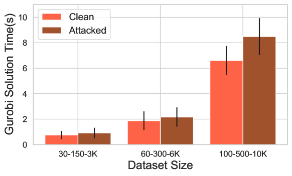
Figure 4: Gurobi’s average time cost (no time limit) in solving clean or attacked MCSCC problems. Experiments are run on 3 datasets (20 instances) of different sizes.

Dataset. There is a lack of large-scale real-world datasets for MCSCC. Thus, we keep the data distribution similar to the MC problem and randomly generate the dataset [20] for training. Specifically, the dataset consists of three configs of set-black element-white element: 30-150-3K, 60-300-6K and 100-500-10K, each with 50 training samples and 10 testing samples. More details about the dataset are presented in Appendix G.

Table 5: Evaluation of solvers for MCSCC (notations are kept in line with MC in Table 4). Since MCSCC incorporates more constraints and is more challenging, our ROCO attackers demonstrate a more significant effect compared to MC, suggesting that solvers may be more vulnerable on CO problems that are inherently more challenging (e.g. with more complicated constraints). The greedy average algorithm is the most robust probably due to its worst-case guarantee known as submodularity [15].

Solver	Problem Size:	Clean Weight $\uparrow$	Attack Method (Attacked Weight)
	#set-#b elem.-#w elem.		Random	ROCO-RA	ROCO-OG	ROCO-SA	ROCO-RL
Local Search	30-150-3K	9.5713	$9.5474\pm 0.0325$	$9.4966\pm 0.0057$	$9.4976\pm 0.0105$	$9.4899\pm 0.0029$	9.4861
Greedy Average	30-150-3K	18.0038	$18.2541\pm 0.1710$	$17.5141\pm 0.0288$	$17.4331\pm 0.0414$	$17.5177\pm 0.0396$	17.1414
Gurobi(1s)	30-150-3K	18.8934	$19.2297\pm 0.1795$	$16.9266\pm 0.2135$	$15.4132\pm 0.3552$	$15.3055\pm 0.3684$	14.2740
Local Search	60-300-6K	24.9913	$25.0413\pm 0.0625$	$24.8738\pm 0.0100$	$\textbf{24.7914}\pm\textbf{0.035}$	$24.8189\pm 0.0375$	$24.8014$
Greedy Average	60-300-6K	43.1625	$43.1539\pm 0.0475$	$42.7697\pm 0.0388$	$42.7611\pm 0.0475$	$42.7222\pm 0.0388$	42.1741
Gurobi(2s)	60-300-6K	41.1828	$41.8005\pm 0.4407$	$38.2382\pm 0.3459$	$37.3322\pm 0.4201$	$38.2918\pm 0.3665$	36.0432
Local Search	100-500-10K	22.9359	$22.9634\pm 0.0482$	$22.7616\pm 0.0206$	$22.6538\pm 0.0183$	$22.7455\pm 0.0206$	22.5804
Greedy Average	100-500-10K	51.3905	$51.4008\pm 0.0308$	$50.7481\pm 0.0719$	$\textbf{50.5169}\pm\textbf{0.1747}$	$50.6865\pm 0.0411$	$50.5631$
Gurobi(5s)	100-500-10K	49.3296	$52.8192\pm 0.3803$	$48.1375\pm 0.3597$	$47.4386\pm 0.4933$	$49.2013\pm 0.2467$	43.4866

Results and analysis. Tab. 5 shows the attack results on our simulated dataset. Both traditional and RL approaches achieve significant attack effects, while RL outperforms the others in most cases (especially for Gurobi). We can see from Tab. 5 that the degradation of Gurobi after attack is much more obvious than that in MC, possibly because the computation progress of MCSCC can include more vulnerable steps than MC. Fig. 4 shows the average time cost (no time limit) for Gurobi in solving MCSCC problems. The figure illustrates that solving time on the attacked instances is longer than those on the clean ones by a large margin, proving the promising power of our attack framework.

Appendix C Graph Embedding for specific Tasks

We discuss specific graph embedding metrics for different kinds of CO problems for reproducibility.

C.1 TASK I: DIRECTED ACYCLIC GRAPH SCHEDULING

Since the task is a directed acyclic graph, we use GCN to encode the state in the original graph and its reverse graph with inversely directed edges separately. Then we concatenate the two node embeddings and use an attention pooling layer to extract the graph-level embedding for Eq. 5:

$$\mathbf{n}=[\mbox{GCN}_{1}(\mathcal{G})||\mbox{GCN}_{2}(\mbox{reverse}(\mathcal{G}))],\ \mathbf{g}=\mbox{AttPool}(\mathbf{n}).$$ (10)

C.2 Task II: Asymmetric Traveling Salesman Problem

Since the graph is fully connected, we use GCN to encode the state in the graph. Then we use an attention pooling layer to extract the graph-level embedding. Eq. 5 becomes:

$$\mathbf{n}=[\mbox{GCN}(\mathcal{G})],\ \mathbf{g}=\mbox{AttPool}(\mathbf{n}).$$ (11)

C.3 Task III: Maximum Coverage

For the RL attack method, different from DAG and ATSP, MC has a unique bipartite graph structure. Therefore, we resort to SAGEConv, which can handle bipartite data, for graph feature extraction. As input, we classify the nodes into two classes (subsets $I_{s}$ and elements $I_{e}$) and associate them with two dimension one-hot tensors. Besides, we add one more dimension for element nodes, which records their weights. Eq. 5 becomes:

$$\mathbf{n}_{e}=\mbox{SAGEConv}_{1}(I_{s},I_{e}) ,\ \mathbf{n}_{s}=\mbox{SAGEConv}_{2}(I_{e},I_{s})$$ (12)

$$\mathbf{g}_{e}=\mbox{AttPool}_{1}(\mathbf{n}_{e}) ,\ \mathbf{g}_{s}=\mbox{AttPool}_{2}(\mathbf{n}_{s})$$

C.4 Task IV: Maximum Coverage with Separate Coverage Constraints

The graph embedding mechanism for MCSCC is exactly the same as MC since they can both be represented by a bipartite graph except that we add one more one-hot dimension to distinguish between black and white elements.

Appendix D Successful Attack Examples

D.1 Task II: Asymmetric Traveling Salesman Problem

A successful attack example is shown in Fig. 5.

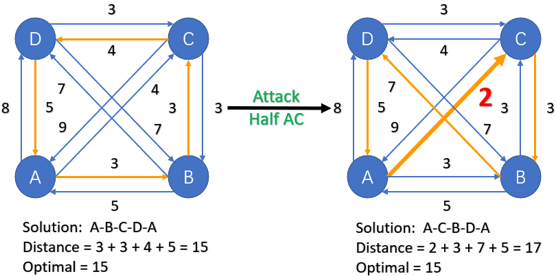
Figure 5: ATSP attack on Nearest Neighbour algorithm. The directed edge represents the distance between two nodes. The attack action on edge AC will cause 2 further distance.

D.2 Task III: Maximum Coverage and Task IV: Maximum Coverage with Separate Coverage Constraints

Successful attack examples are shown in Fig. 6.

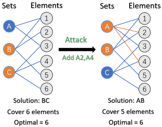
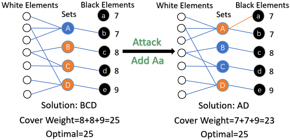
Figure 6: Left: MC attack on Greedy algorithm. The threshold $k$ of the sets is 2 and all the elements have unit weight. Attacks on edges A2 and A4 will cause a lower covered weight. Right: MCSCC attack on Greedy Average algorithm. The threshold $k$ of the white elements is $5$ and the value near the black element represents its weight. Attack on edge Aa causes a lower covered black element weight.

Appendix E Formulas and Proofs

E.1 MCSCC NP-hard Provement

We prove that the decision problem of MCSCC is NP-complete, thus the optimization problem of MCSCC in our paper is NP-hard. For the sake of our proof, here we redefine MCSCC and give definition of a traditional NP-Complete problem: Set Covering.

The decision problem of MCSCC. Given a series of sets $\mathcal{R}=\{R_{1},R_{2},...,R_{n}\}$ along with an element set consisted of white and black elements $\mathcal{E}=\mathcal{W}\cup\mathcal{B}$. The sets cover certain elements (white $C^{-}(R_{i})$ or black $C^{+}(R_{i})$) which have their weights $w(e)$. Does there exist a collection of these sets $\mathcal{R}^{\prime}\subseteq\mathcal{R}$ to cover $\geq M$ black elements weight while influence no more than $k$ white elements?

Set Covering. Given a set $U$ of elements, a collection $S_{1},S_{2},\dots,S_{n}$ of subsets of $U$, and an integer $k$, does there exist a collection of $\leq k$ of these sets whose union is equal to $U$?

First, we need to show that MCSCC is NP. Given a collection of selected sets $\mathcal{R}^{\prime}=\{R_{1},R_{2},\dots,R_{m}\}$, we can simply traverse the set, recording the covered black and white elements. Then, we can assert whether the covered black element number is no more than $k$ and fraudulent monetary value is no less than $m$.

Since the certification process can be done in $O(n^{2})$, we can tell that MCSCC is NP. Then, for NP-hardness, we can get it reduced from Set Covering.

Suppose we have a Set Covering instance, we construct an equivalent MCSCC problem as follows:

• Create $|U|$ black elements with weight 1, corresponding to elements in Set Covering.

• Create $n$ sets, set $C^{+}(R_{i})=S_{i}$.

• Connect each set to a different white element of weight 1.

• Set the white element threshold $k_{w}$ equal to the set number threshold $k_{s}$.

• Set black element weight target $M=|U|$.

Suppose we find a collection of sets which meet the conditions of MCSCC, then we select subsets in Set Covering $S_{i}$ iff we select $R_{i}$. The total number of subsets is no more than $k_{w}(k_{s})$ since the influenced white element number is equal to $|\mathcal{R}^{\prime}|$. The subsets also cover $U$ since the covered black element weight (each with amount 1) is no less than $|U|$. Similarly, we can prove that we can find a suitable subset collection for MCSCC if we have found a collection of subsets that meet the conditions of Set Covering. So we can induce that $\textbf{Set Covering}\leq_{p}\textbf{MCSCC}$.

Thus, we have proved that the decision problem of MCSCC is NP-Complete.

E.2 MCSCC ILP Formulation

As discussed in the main text, $\mathcal{B}$ denotes the set of black elements, $\mathcal{W}$ represents the set of white elements, $\mathcal{S}$ refers to the collection of sets and $\mathcal{E}$ denotes the element set. Using notations above, we can translate Eq. 9 into standard ILP form as follows:

$$\max\ \sum_{i\in\mathcal{B}} Y[i]\times W[i],\quad s.t.\ \sum_{i\in\mathcal{W}}Y[i]\leq k$$ (13)

$$\mbox{for}\ i=1\dots|\mathcal{E}|, (Y[i]-0.5)(0.5-\sum_{j=1}^{|\mathcal{R}|}X[j]\times\mathbb{I}(i\ \mbox{in}\ E[j]))\leq 0$$

where $X[j]\in\{0,1\}$ denotes set $S_{j}$ is chosen (1) or not (0), $Y[i]\in\{0,1\}$ shows whether element $i$ has been covered by the chosen sets. Besides, $W[i]\in\mathbb{R}$ records the weight of the elements while $E[j]\subseteq\mathcal{E}$ is the corresponding elements of set $S_{j}$. The third equation ensures the element binary variable $Y[i]$ to be $1$ iff it has been covered by a certain set (if $\exists X[j]=1$ and element $i\in E[j]$, then the formula in the second bracket is negative, ensuring $Y[i]$ to be 1; else if element $i$ is not covered by any chosen sets, then the second formula is positive and $Y[i]$ must be 0).

Appendix F Calibrated Time

Considering the instability of the server and the interference of other running programs, calibrated time is designed to evaluate the server speed within a small period of time. Specifically, we define the speed as the reciprocal of the Wall clock time to solve a given calibration MIP. The calibration MIP is generated in the stable condition and solved $K$ times to record the basic speed $\text{speed}_{base}$. When evaluating the other instances, we will first evaluate the calibration MIP $K$ times to calculate the current speed $\text{speed}_{now}$. $K$ is the number of samples, which is set as $20$ in our experiments.

To fairly measure the solvers’ performance under different computational resources, take MC problems as an example, a given calibration MIP is also a specified MC problem to design time limits for different server speeds. Specifically, the new time limit for the solver will be set as:

$$\text{New Time Limit}=\frac{\text{speed}_{base}}{\text{speed}_{now}}\times\text{Uniform Time Limit}$$ (14)

Appendix G MCSCC Dataset

Besides the distribution rules of MC, we generate the MCSCC dataset mainly by the following two rules: 1) The black element weights are uniformly distributed in the range $[0,1]$. 2) The number of black elements is 5% of white elements. 3) The covered black element weights and wight element numbers of sets follow a Gaussian distribution with a large standard deviation, to enlarge the differences between the sets.

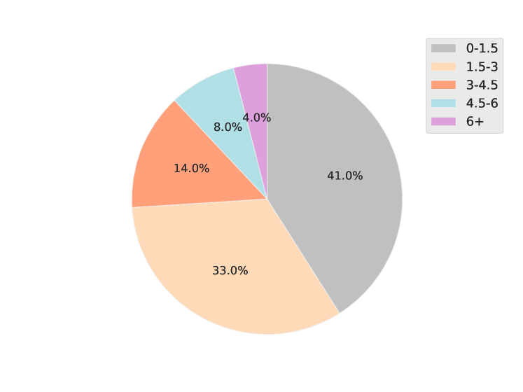
Figure 7: The distribution of black element weights covered by different sets. The $x-y$ pair in legends means the set can cover weights in range $[x,y]$.

Fig. 7 shows the black element weights covered by different sets in a 100-500-10K problem instance. As we can see, few well-designed sets can cover most weights while the others can be regarded as complementary to these sets. This design enlarges the difference between the different quality of solutions, therefore promoting the potential to be attacked.

Appendix H Experiment Setups

Experiment environments. DAG and ATSP experiments are run on a GeForce RTX 2080Ti while MC and MCSCC experiments are run on a GeForce RTX 3090 (20GB). We implement our models with Python 3.7, PyTorch 1.9.0 and PyTorch Geometric 1.7.2.

RL settings. Tab. 6 records the hyperparameters for RL during the training process. Trust region clip factor is a parameter in PPO agent to avoid model collapse. We also adopt some common policy-gradient training tricks like reward normalization and entropy regularization during training processes.

Table 6: RL parameter configuration in tasks DAG, ATSP, MC and MCSCC

Parameters	DAG	ATSP	MC & MCSCC
Actions#	20	20	10
Reward discount factor	0.95	0.95	0.95
Trust region clip factor	0.1	0.1	0.1
GNN type	GCN	GCN	SAGEConv
GNN layers#	5	3	3
Learning rate	1e-4	1e-3	1e-3
Node feature dimensions#	64	20	16

Table 7: Comparison of our attackers. Randomness means it will produce different results in different trials. Trained means whether the parameters are tuned by a training set.

Attack Method	Randomness	Trained	Time Complexity
ROCO-RA	$\checkmark$		$O(NK)$
ROCO-OG	$\checkmark$		$O(BMK)$
ROCO-SA	$\checkmark$	$\checkmark$	$O(NMK)$
ROCO-RL		$\checkmark$	$O(B^{2}K)$

Attacker hyperparameters. For fair comparison of different attackers and the consideration of RL inference time, the hyperparameters are set to ensure similar evaluation time across different attack methods. According to the time complexity we calculate in Tab. 7, here we specify the following parameters: number of iterations $N$, beam search size $B$ and number of different actions $M$ in each iteration.

• DAG : ROCO-RA $N=30$; ROCO-OG $B=3$, $M=9$; ROCO-SA $N=5$, $M=6$; ROCO-RL $B=3$.

• ATSP : ROCO-RA $N=130$; ROCO-OG $B=5$, $M=25$; ROCO-SA $N=13$, $M=10$; ROCO-RL $B=5$.

• MC : ROCO-RA $N=220$; ROCO-OG $B=6$, $M=36$; ROCO-SA $N=22$, $M=10$; ROCO-RL $B=6$.

• MCSCC : ROCO-RA $N=250$; ROCO-OG $B=6$, $M=36$; ROCO-SA $N=25$, $M=10$; ROCO-RL $B=6$.

Appendix I Discussion about Limitations and Potential Negative Impacts

Limitations.

First of all, as our framework is designed for combinatorial optimization problems on graphs, it needs non-trivial reformulation to fit into CO problems cannot encoded by graphs. Secondly, the principle of designing our attack action is based on the graph modification to achieve no-worse optimum, which may not be applicable to all CO problems.

Potential Negative Impacts.

As we propose the first general framework to evaluate the robustness of combinatorial solvers on graphs, this may be used by unscrupulous people to attack different solvers, increasing the burden on engineers to cope with the malicious attacks.

References

- [1] Y. Bengio, A. Lodi, and A. Prouvost. Machine learning for combinatorial optimization: a methodological tour d’horizon. EJOR, 2021.
- [2] C. Buchheim and J. Kurtz. Robust combinatorial optimization under convex and discrete cost uncertainty. EURO Journal on Computational Optimization, 6(3):211–238, 2018.
- [3] N. Carlini and D. A. Wagner. Towards evaluating the robustness of neural networks. IEEE Symposium on Security and Privacy (SP), 2017.
- [4] C. Chambers, A. Raniwala, F. Perry, S. Adams, R. R. Henry, R. Bradshaw, and N. Weizenbaum. Flumejava: easy, efficient data-parallel pipelines. ACM Sigplan Notices, 45(6):363–375, 2010.
- [5] J. Cirasella, D. S. Johnson, L. A. McGeoch, and W. Zhang. The asymmetric traveling salesman problem: Algorithms, instance generators, and tests. In Workshop on Algorithm Engineering and Experimentation, 2001.
- [6] H. Dai, H. Li, T. Tian, X. Huang, L. Wang, J. Zhu, and L. Song. Adversarial attack on graph structured data. In ICML, 2018.
- [7] U. Feige. A threshold of ln n for approximating set cover. J. ACM, 45(4):634–652, jul 1998.
- [8] J. Forrest, T. Ralphs, H. G. Santos, S. Vigerske, L. Hafer, J. Forrest, B. Kristjansson, jpfasano, EdwinStraver, M. Lubin, rlougee, jpgoncal1, Jan-Willem, h-i gassmann, S. Brito, Cristina, M. Saltzman, tosttost, F. MATSUSHIMA, and to st. coin-or/cbc: Release releases/2.10.7, Jan. 2022.
- [9] S. Geisler, J. Sommer, J. Schuchardt, A. Bojchevski, and S. Günnemann. Generalization of neural combinatorial solvers through the lens of adversarial robustness. arXiv:2110.10942, 2021.
- [10] I. J. Goodfellow, J. Shlens, and C. Szegedy. Explaining and harnessing adversarial examples. In ICLR, 2015.
- [11] R. Grandl, G. Ananthanarayanan, S. Kandula, S. Rao, and A. Akella. Multi-resource packing for cluster schedulers. ACM SIGCOMM Computer Communication Review, 44(4):455–466, 2014.
- [12] Gurobi Optimization. Gurobi optimizer reference manual. http://www.gurobi.com, 2020.
- [13] K. He, X. Zhang, S. Ren, and J. Sun. Deep residual learning for image recognition. In CVPR, 2016.
- [14] K. Helsgaun. An extension of the lin-kernighan-helsgaun tsp solver for constrained traveling salesman and vehicle routing problems. Roskilde: Roskilde University, 2017.
- [15] D. S. Hochbaum. Approximating Covering and Packing Problems: Set Cover, Vertex Cover, Independent Set, and Related Problems, page 94–143. PWS Publishing Co., USA, 1996.
- [16] A. Ilyas, L. Engstrom, A. Athalye, and J. Lin. Black-box adversarial attacks with limited queries and information. In ICML, 2018.
- [17] R. Jia and P. Liang. Adversarial examples for evaluating reading comprehension systems. In EMNLP, 2017.
- [18] E. Khalil, H. Dai, Y. Zhang, B. Dilkina, and L. Song. Learning combinatorial optimization algorithms over graphs. In NeurIPS, 2017.
- [19] T. N. Kipf and M. Welling. Semi-supervised classification with graph convolutional networks. arXiv:1609.02907, 2016.
- [20] Y.-D. Kwon, J. Choo, I. Yoon, M. Park, D. Park, and Y. Gwon. Matrix encoding networks for neural combinatorial optimization. arXiv:2106.11113, 2021.
- [21] G. Lyu, S. Feng, and Y. Li. Partial multi-label learning via probabilistic graph matching mechanism. In Proceedings of the 26th ACM SIGKDD International Conference on Knowledge Discovery & Data Mining, pages 105–113, 2020.
- [22] A. Madry, A. Makelov, L. Schmidt, D. Tsipras, and A. Vladu. Towards deep learning models resistant to adversarial attacks. In ICLR, 2018.
- [23] H. Mao, M. Schwarzkopf, S. B. Venkatakrishnan, Z. Meng, and M. Alizadeh. Learning scheduling algorithms for data processing clusters. In Proceedings of the ACM Special Interest Group on Data Communication, pages 270–288. 2019.
- [24] V. Nair, S. Bartunov, F. Gimeno, I. von Glehn, P. Lichocki, I. Lobov, B. O’Donoghue, N. Sonnerat, C. Tjandraatmadja, P. Wang, et al. Solving mixed integer programs using neural networks. arXiv:2012.13349, 2020.
- [25] N. Narodytska and S. P. Kasiviswanathan. Simple black-box adversarial perturbations for deep networks. arXiv:1612.06299, 2016.
- [26] M. V. Pogančić, A. Paulus, V. Musil, G. Martius, and M. Rolinek. Differentiation of blackbox combinatorial solvers. In ICLR, 2019.
- [27] J. Ren, Z. Zhang, J. Jin, X. Zhao, S. Wu, Y. Zhou, Y. Shen, T. Che, R. Jin, and D. Dou. Integrated defense for resilient graph matching. In ICML, 2021.
- [28] B. Saha, H. Shah, S. Seth, G. Vijayaraghavan, A. Murthy, and C. Curino. Apache tez: A unifying framework for modeling and building data processing applications. In ACM SIGMOD, 2015.
- [29] F. Scarselli, M. Gori, A. C. Tsoi, M. Hagenbuchner, and G. Monfardini. The graph neural network model. IEEE transactions on neural networks, 20(1):61–80, 2008.
- [30] J. Schulman, F. Wolski, P. Dhariwal, A. Radford, and O. Klimov. Proximal policy optimization algorithms. arXiv:1707.06347, 2017.
- [31] C. Szegedy, W. Zaremba, I. Sutskever, J. Bruna, D. Erhan, I. Goodfellow, and R. Fergus. Intriguing properties of neural networks. arXiv:1312.6199, 2014.
- [32] The SCIP Optimization Suite 8.0, 2021.
- [33] P. J. Van Laarhoven and E. H. Aarts. Simulated annealing. In Simulated annealing: Theory and applications, pages 7–15. Springer, 1987.
- [34] N. Varma and Y. Yoshida. Average sensitivity of graph algorithms. In SODA, 2021.
- [35] P. Velickovic, G. Cucurull, A. Casanova, A. Romero, P. Lio, and Y. Bengio. Graph attention networks. stat, 1050:20, 2017.
- [36] O. Vinyals, M. Fortunato, and N. Jaitly. Pointer networks. In NeurIPS, 2015.
- [37] R. Wang, Z. Hua, G. Liu, J. Zhang, J. Yan, F. Qi, S. Yang, J. Zhou, and X. Yang. A bi-level framework for learning to solve combinatorial optimization on graphs. In NeurIPS, 2021.
- [38] D. Whitley. A genetic algorithm tutorial. Statistics and computing, 4(2):65–85, 1994.
- [39] G. Yehuda, M. Gabel, and A. Schuster. It’s not what machines can learn, it’s what we cannot teach. In ICML, 2020.
- [40] M. Zaharia, M. Chowdhury, T. Das, A. Dave, J. Ma, M. McCauly, M. J. Franklin, S. Shenker, and I. Stoica. Resilient distributed datasets: A fault-tolerant abstraction for in-memory cluster computing. In NSDI, 2012.
- [41] X. Zhang, F. Qi, Z. Hua, and S. Yang. Solving billion-scale knapsack problems. In Proceedings of The Web Conference 2020, pages 3105–3111, 2020.
- [42] Z. Zhang, Z. Zhang, Y. Zhou, Y. Shen, R. Jin, and D. Dou. Adversarial attacks on deep graph matching. In NeurIPS, 2020.
- [43] J. Zhu, J. Zhu, S. Ghosh, W. Wu, and J. Yuan. Social influence maximization in hypergraph in social networks. IEEE Transactions on Network Science and Engineering, 6(4):801–811, 2019.