Radio Pulsar Sub-Populations (II) : The Mysterious RRATs

Abstract

Several conjectures have been put forward to explain the RRATs, the newest subclass of neutron stars, and their connections to other radio pulsars. This work discusses these conjectures in the context of the characteristic properties of the RRAT population. Contrary to expectations, it is seen that - a) the RRAT population is statistically un-correlated with the nulling pulsars, and b) the RRAT phenomenon is unlikely to be related to old age or death-line proximity. It is perhaps more likely that the special emission property of RRATs is a signature of them being later evolutionary phases of other types of neutron stars which may have resulted in restructuring of the magnetic fields.

sushan.konar@gmail.com

12.3456/s78910-011-012-3 #### 000 0000 1– 1

1 Introduction

Close to $\sim$3500 neutron stars have been observed and investigated (in varying detail) since the serendipitous discovery of PSR B1919+21 in 1967 [Hewish et al. (1968)]. Most of these neutron stars are observed as Radio Pulsars, characterized by short spin-periods ($\sim 10^{-3}-10^{2}$ s) and large inferred surface magnetic fields ($\sim 10^{8}-10^{15}$ G). These rotation powered pulsars (RPP) are mostly isolated, or are members of binaries where active mass transfer is not currently taking place [Kaspi (2010), Konar (2013), Konar et al. (2016), Konar (2017)].

The main characteristic feature of a radio pulsar (RPSR) is the emission of highly coherent radiation (across a wide range of the electromagnetic frequency spectrum) observed as regular periodic pulses. However, the process of emission is seen to deviate from a regular pattern in a significant number of RPSRs. One such irregularity is the phenomenon of nulling, first detected by ?) and now seen in $\sim$200 pulsars, which refers to the abrupt cessation of pulsed emission for a number of (can vary from a few to hundreds or even thousands) pulse periods. In an earlier work, we have discussed the population of Nulling Pulsars (NPSRs) in detail ([Konar & Deka (2019)] - Paper-I hereafter).

However, the extreme case of irregular emission is displayed by a group of objects known as Rotating Radio Transients (RRAT). In 2006, eleven new radio transient sources were discovered in the Parkes Multi-beam Pulsar Survey [McLaughlin et al. (2006)]. The duration of their radio bursts were $\sim$2-30 ms and the intervals between the bursts ranged from minutes to hours. None of these were detectable in periodicity searches and appeared only via single pulse searches. The primary characteristic of these transients appeared to be sporadic single pulse emissions at constant dispersion measures (DM); with underlying periodicities suggestive of a neutron star origin.

In this discovery paper, it was conjectured that the RRATs represented a distinct and previously unknown class of neutron stars and were defined to be radio pulsars which can only be detected through single-pulse searches. Alternatively, ?) defined an RRAT as a pulsar which predominantly emits isolated pulses. However, many argued that the RRAT behaviour was only an extreme case of pulsar nulling/intermittency and required no separate identification. The justification for this argument comes from the fact that the log-normal pulse distributions and power-law frequency dependence of the mean flux are both consistent with those for the ordinary RPSRs (unlike Magnetars or giant pulses from RPSRs). This is a clear indication of the RRATs being a subclass of Radio Pulsars whatever may be the reason for their unusual emission characteristics.

Nevertheless, with rapidly increasing number of RRAT detections, a clear-cut definition for these objects became essential. So, ?) proposed the following - “A RRAT is a repeating radio source, with underlying periodicity, which is more significantly detectable via its single pulses than in periodicity searches.” Clearly, this definition comes with a caveat. Because, a pulsar may appear RRAT-like in a certain observational set-up but not in another. Notwithstanding the caveat, all detections identified as RRATs till then [McLaughlin et al. (2006), Hessels et al. (2008), Shitov et al. (2009), Keane et al. (2010), Burke-Spolaor & Bailes (2010), Keane et al. (2011), Burke-Spolaor et al. (2011)] and later observational campaigns have used the same definition. Current public databases, like the ‘ATNF Pulsar Catalog’ or ‘The RRATalog’, also use this same criterion to classify objects as RRATs. In the present work, RRAT data has primarily been taken from these public databases. Therefore, here too RRAT has the same meaning as the definition above.

Assuming these to represent a distinct sub-population of neutron stars, ?) estimated that the RRATs are expected to be significantly more numerous (by a factor of 3 or 4) than ‘normal’ pulsars (typically detected through periodicity searches). Even if we accept this to be an over-estimate (given the uncertainties implicit in various factors), the implication is quite serious. On the basis of their estimates of the numbers and birthrates of Galactic neutron stars, ?) demonstrated that treating the normal pulsars, the RRATs, the XDINS (X-ray Dim Isolated Neutron Stars), the Magnetars, and the CCOs (Central Compact Objects) as distinct sub-classes of neutron stars would not be not consistent with the observed Galactic supernova rate (required to be greater than or equal to total neutron star birthrate). [See ?) and ?) for discussions on these observationally distinct sub-populations of neutron stars.]

This inconsistency is suggestive of connections (evolutionary or otherwise) between distinct sub-populations of neutron stars. To explain the ‘RRAT phenomenon’ (specifically, the nature of their transient radio emission) a number of hypotheses have been suggested. Most of these hypotheses have direct bearings on the connection of RRATs with other neutron star sub-populations. For many of these hypotheses, there exist tentative observational support. But, as yet, none of them prove to be definitive.

Bearing these in mind, we consider the characteristics of the RRAT population as a whole and examine some of these hypotheses. The basic characteristics of the RRAT population are discussed in §2. In §3, we concentrate upon the question of the connection of the RRATs with the NPSRs, by comparing these two populations, in view of the results obtained in Paper-I. In §4, we consider the question of the proximity of the RRATs and the NPSRs to the death-line. A few other hypotheses regarding the nature of RRATs are examined in §5 and we summarise our conclusions in §6.

2 RRAT Population

So far 162 RRATs (listed in Table-[5-8]) have been found through archival and direct pulsar surveys since their discovery [McLaughlin et al. (2006)]. Even though RRAT emission has an underlying periodicity, the interval between individual pulses can widely vary, depending upon the epoch. Because of this, the spin-period of an RRAT is determined by finding the greatest common denominator of the intervals between pulses. Clearly, this method is likely to yield a multiple of the period instead of the true one, unless more than a few pulses have been detected in an observation [Cui et al. (2017)]. This problem is usually taken care of by detecting sufficiently large number of pulses from a particular RRAT to arrive at the true period of the neutron star.

To date, the population of RRATs has been seen to have the following ranges for the spin-period (P_s), the dipolar surface magnetic field (B_s), and the dispersion measure (DM) –

• P_S : 41.5 ms – 7.7 s ;

• B_s : 1.67 $\times 10^{11}$ – 4.96 $\times 10^{13}$ G;

• DM : 4.0 – 786.0 pc.cm^-3.

Understandably, timing measurements are difficult and values for the spin-period or the period derivative (hence, estimates for the dipolar surface magnetic field) are not available for all of the known RRATs. In Fig.[1], the RRATs (for which both P_s and B_s values are available) have been shown, along with the NPSRs and other non-nulling RPSRs, in the P_s-B_s plot. A P_s histogram, for the RRATs that do not have known values of B_s, is also provided at the bottom of Fig.[1] to indicate the general trend for P_s values. It is seen that the spin-period and the surface magnetic field values of RRATs are skewed towards the higher side compared to those for the normal RPSR population (millisecond pulsars excluded). It is also noted that many RRATs occupy the same region of the P_s-B_s plane where some Magnetars have been found [Cui et al. (2017)].

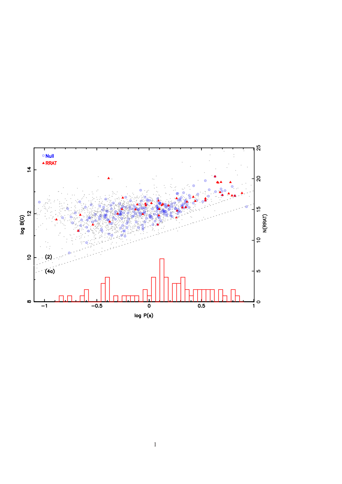
Figure 1: Distribution of known RRATs (red triangles) and NPSRs (circled dots in blue) along-with normal RPSRs (grey dots) in the P_s–B_s plane. 214 NPSRs (of the 222 known) and 42 RRATs (of the 162 known), with estimates of B_s, are shown here. The P_s histogram at the bottom corresponds to another 67 RRATs, for which only P_s values are available. The y-axis on the right shows the number of objects corresponding to this RRAT histogram. The grey dashed lines, marked ‘(2)’ and ‘(4a)’ correspond to two theoretical death-lines (see text for details).
Data : a) Normal Pulsars - ATNF Pulsar Catalogue, b) RRAT - Appendix A,
c) NPSR - Null Catalogue (Paper-I : http://www.ncra.tifr.res.in/$\sim$sushan/null/null.html).

Now, the basic requirement for pulsar emission is a copious amount of pair production in the magnetosphere of the neutron star. Pulsars ‘switch off’ when conditions for pair production fail to be met. ?) was the first to define a cut-off line (known as the death-line now) for pulsar emission in the context of the NPSRs. It was conjectured that the NPSRs experience null simply because of their proximity to the death-line. Over the years, the theory of death-lines has been investigated in detail. In Paper-I we have discussed the significance of a number of death-lines that have been proposed, in the light of the current pulsar data. It is noticed that two of the death-lines developed by ?) are of importance for the RPSR population as a whole, and the NPSRs in particular.

Both of these death-lines are obtained assuming the pair productions ($\gamma+B\rightarrow e^{-}+e^{+}$, $\gamma$ - photon, $e^{-/+}$ - electron/positron, B - magnetic field) to occur predominantly near the polar cap of the neutron star [Ruderman & Sutherland (1975)]. It is also assumed that a) the surface field is dipolar, and b) the radius of curvature for the magnetic field is approximately equal to the stellar radius. These death-lines, numbered as [2] and [4a] in Paper-I are as follows -

[2] : $$4\log B_{s}-6.5\log P_{s}=45.7\,,$$ (1)

[4a] : $$4\log B_{s}-6\log P_{s}=43.8\,;$$ (2)

where P_s is in seconds and B_s is in Gauss. Death-line [2] corresponds to the case of very curved field lines whereas [4a] is obtained for extremely twisted field lines. It is clearly seen from Fig.[1] that the region beyond death-line [4a] is almost empty. However, the RRATs and the NPSRs are almost entirely bounded below by the death-line [2], suggesting similarities / connections between these two populations.

3 RRAT-NPSR Connection

Because of their intermittent nature it has been natural to look for similarities and/or connections between the RRATs and the NPSRs. ?) considered this issue in detail and concluded that RRATs are likely to be ‘extreme’ cases of NPSRs. They found that PSR J0941-39 switches between a RRAT-like and an NPSR-like mode, i.e. sometimes appearing with a sporadic RRAT-like emission and at other times emitting as a bright regular nulling pulsar. Noting that this object may represent a direct link between ordinary pulsars and RRATs they suggested that RRATs could be an evolutionary phase of pulsars with a high nulling fraction (NF - fraction of time a pulsar is not seen in emission) or nulling pulsars that ‘switch on’ for less than the duration of a pulse period.

An object of interest in this context is PSR J1107-5907, known to have many different modes of emission - a strong mode with a broad profile with nulls, a weak mode with a narrow profile that has occasional bursts of up to a few clearly detectable pulses at a time, and a low-level underlying emission. It has been argued that this source would look like an RRAT for most of the time, if placed at a larger distance [Young et al. (2014)]. A very similar conjecture has also been made about another NPSR (B0656+14/J0659+1414) that it would have appeared RRAT-like if located at a greater distance [Weltevrede et al. (2006)]. J1107-5907 also exhibits different NFs in different emission modes, similar to that observed in B0826-34 (J0828-3417) and J0941-39, both of which appear to switch between an RRAT-like and a more typical ‘pulsar-like’ phase [Burke-Spolaor & Bailes (2010), Burke-Spolaor et al. (2012), Esamdin et al. (2012)].

Then again, the weak emission mode of B0826-34 is liable to be confused with nulling phases if the signal is not integrated over a sufficiently long interval of time. This has been suggested to be indicative of an evolutionary progression towards the death-line; and that all (or most) pulsars likely start off as continuous emitters, gradually begin to null and then increase their NF to become RRATs, ultimately crossing the death-line to end the active radio emission phase [Burke-Spolaor & Bailes (2010)]. In fact, both J1107-5907 and B0826-34 are quite close to the death line. However, there also exist a large number of NPSRs that are close to the death-line but are not known to exhibit any RRAT-like behaviour. Similarly, quite a few RRATs are found far away from the death-line (see Fig.1). Therefore, death-line proximity does not immediately imply a certain nature of pulsar emission. We discuss this issue in detail in §3.

	Ps	Bs	$\tau_{c}$	DM
	s	1012 G	107 yr	pc.cm-3
RRAT	2.07	7.18	1.59	105.91
N	109	44	44	162
NPSR	1.26	2.63	3.99	134.78
N	222	215	215	222
ALL	1.53	3.40	3.58	122.60
N	331	259	259	384

Table 1: Average values of P_s, B_s, $\tau_{c}$ and DM for the RRAT, the NPSR and the combined populations. The rows marked ‘N’ indicate the number of objects for which values of the corresponding parameter are available and have therefore been used to calculate the average. NPSRs also include the intermittent pulsars. Data : a) RRAT - Appendix A, b) NPSR - Null Catalogue.

Even though the picture is not yet clear, it is evident that there exist certain connections between the RRATs and the NPSRs. Clear nulling segments were also exhibited recently by another RRAT (J1913+1330) in a FAST observation [Lu et al. (2019)]. At this point, some other objects have also been observed to exhibit such RRAT-NPSR ‘dual’ nature (see Table-[4]). To understand this connection better, we look at the statistical nature of the RRAT and the NPSR populations below.

Table-[1] summarises the average values of relevant physical quantities of the RRAT and the NPSR populations. Clearly, the RRATs have larger average spin-periods, and larger average surface magnetic fields, as has already been remarked upon. Consequently, NPSRs have larger characteristic ages ($\tau_{c}$) compared to the RRATs (B_s$\sim$$\sqrt{{\rm P}_{s}\mbox{$\dot{\rm P}_{s}$}}$, $\tau_{c}$$\sim$${\rm P}_{s}/\mbox{$\dot{\rm P}_{s}$}$). We must remember that the estimate of characteristic age is crucially dependent on the assumption of a constant magnetic field, which may or may not be applicable to RRATs. However, RRATs clearly have lower average DM, indicating that they are not necessarily located farther away compared to the NPSRs. Therefore, the conjecture that a distant NPSR might appear to be RRAT-like is unlikely to explain the majority of objects, even if such a situation is realised for a small number of the RRATs.

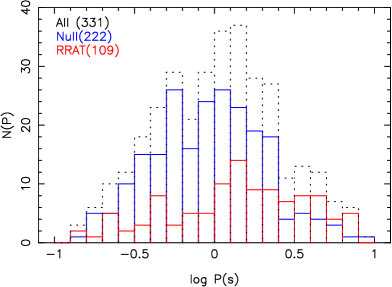
Figure 2: P_s distribution of the RRATs (red), the NPSRs (blue) and the combined (NPSR + RRAT) population (black broken line). Number of objects (data points) available for each distribution is shown within brackets.

Fig.2–4 show the distribution histograms of these parameters. In order to quantify the nature of the distributions, we perform 1-sample Kolmogorov-Smirnov [von Mises (1980)] tests on each set of data. The results are summarised in Table-[3]. It is seen that P_KS, the probability of error for rejecting the hypothesis that the data is normally distributed, is very high for $\log({\rm P}_{s})$ and $\log({\rm B}_{s})$ but tiny for DM for both RRAT and NPSR populations (P_s in units of second and B_s in units of Gauss). Clearly, $\log({\rm P}_{s})$ and $\log({\rm B}_{s})$ are expected to be normally distributed. In other words, P_s and B_s are log-normally distributed for both the populations, though with somewhat different degree of normality. We also perform the 2-population Kolmogorov-Smirnov tests on the parameter values to compare the RRAT and the NPSR populations. The bottom panel of Table-[3] show the results. It is obvious that the statistical distributions of P_s, B_s for RRATs and NPSRs are completely dissimilar.

The combined distributions, for both of these parameters, are also log-normally distributed with a degree of normality in-between the RRAT and the NPSR distributions. This could be due to the fact that the size of the NPSR population is much bigger (twice for P_s and five times for B_s values) than the RRAT population and the behaviour of the combined population is basically dictated by that of the NPSRs. It might be tempting to conclude that the NPSRs and the RRATs come from two different segments of the same underlying population which is Gaussian in nature. But the fact that both the RRAT and the NPSR parameters also tend to be separately Gaussian contradicts such a conclusion.

As expected, the nature of the DM distribution is very different. Given that the dispersion measure can be considered to be a proxy for distance (with certain caveats) a normal distribution is not really expected. Because every detection is limited by the inherent sensitivity of the particular observation and nearer sources are expected to be detected with a higher probability. But it is surprising to note that the DM distributions of the NPSRs and the RRATs are totally dissimilar (P_KS(R-N) $<10^{-2}$). As both the RRATs and the NPSRs are being detected by same/similar observational instruments, we can interpret this result in two ways - either, a) the single pulse searches (detecting RRATs) are more sensitive at low DM compared to the periodicity searches (detecting regular pulsars), or b) for any given detection sensitivity only RRATs located at shorter distances are detected. The second possibility, suggestive of a scenario where the ‘RRAT phenomenon’ is observed only for nearby neutron stars, is problematic as it exacerbates the ‘birthrate problem’ discussed earlier.

In summary, the current populations of the RRATs and the NPSRs can not be said to belong to the same sub-class of RPSRs. Therefore, while the observations clearly suggest that they have certain inherent connections, it would perhaps not be accurate to treat the RRAT emission simply as an extreme form of nulling behaviour.

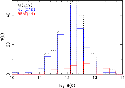
Figure 3: B_s distribution of the RRATs (red), the NPSRs and the combined distribution (black broken line).

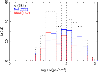
Figure 4: DM distribution of the RRATs (red), the NPSRs and the combined distribution (black broken line).

	log(Ps/s)	log(Bs/G)	DM
RRAT
PKS(N)	0.36	0.93	$<10^{-5}$
DKS(N)	0.08	0.07	0.23
N	109	44	162
NPSR
PKS(N)	0.70	0.55	$<10^{-5}$
DKS(N)	0.05	0.05	0.17
N	222	215	222
ALL
PKS(N)	0.47	0.63	$<10^{-5}$
DKS(N)	0.05	0.05	0.19
N	331	259	384
KS2 : RRAT vs. NPSR
PKS(R-N)	$<10^{-3}$	$<10^{-3}$	$\sim 10^{-2}$
DKS(R-N)	0.25	0.33	0.17
N	109,222	44,215	162,222

Table 2: Kolmogorov-Smirnov test statistics : P_KS(N) is the probability of error for rejecting the null hypothesis that the sample is normally distributed, and D_KS(N) is the magnitude of the difference between the sample distribution and the normal distribution. The tests are performed on $\log$(P_s), $\log$(B_s) and DM. P_KS(R-N) & D_KS(R-N) are the corresponding quantities for the null hypothesis that both the RRATs and the NPSRs are drawn from the same underlying population. Data : a) RRAT - Appendix A, b) NPSR - Null Catalogue.

4 Death-Line Proximity

It has been suggested that the RRATs could be RPSRs close to the pulsar death line in the P_s-B_s plane. These systems might be emitting weak, continuous radio pulses, which have not been detected yet, in addition to the observed short radio bursts [Weltevrede et al. (2006)].

To check if the RRAT phenomenon is connected to a proximity to the death-line, we define a proximity parameter, $\epsilon$, given by -

$$\epsilon=\frac{\tau_{D}-\tau_{c}}{\tau_{D}}\,,$$ (3)

where, $\tau_{c}$ is the current (characteristic) age of a pulsar given by P_s/2$\dot{\rm P}_{s}$. This definition of $\tau_{c}$ inherently assumes that - a) the pulsar has P_s $\sim$0 at birth, and b) B_s does not evolve significantly over the active lifetime of a pulsar. This constant surface magnetic field of a pulsar is obtained using the measured values of P_s and $\dot{\rm P}_{s}$ from the relation -

$$B_{s}=3.2\times 10^{19}\sqrt{{\rm P}_{s}\dot{\rm P}}\,\,\mbox{G}\,,$$ (4)

where P_s is in seconds and $\dot{\rm P}_{s}$ is in $ss^{-1}$, assuming a purely dipolar field.

Under the same assumptions mentioned above $\tau_{D}$ is defined to be the total time taken by a pulsar to reach the death line, such that

$$\tau_{D}=\frac{{\rm P}_{D}}{2\dot{{\rm P}}_{D}}\,,$$ (5)

where P_D is the spin-period at death line and $\dot{\rm P}$_D is the period derivative at the death-line. Clearly, the definition of $\tau_{D}$ depends on a particular choice of the death-line. In this work, we adopt death-line [2], given by Eq.(1). This gives us the following expressions for P_D and $\dot{\rm P}$_D -

$$\log{\rm P}_{D}=0.62\log{\rm B}_{s}-7.03\,,$$ (6)

$$\dot{\rm P}_{D}=9.76\times 10^{-39}{\rm P}_{D}^{-1}\,{\rm B}^{2}_{s}\,;$$ (7)

where P_D is in seconds, $\dot{\rm P}$_D is in $ss^{-1}$, and B_s is in G. The distribution histograms of P_D and $\epsilon$, for the corresponding populations are shown in Fig.5 - 7.

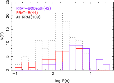
Figure 5: Distribution of P_s (red) for RRATs with available B_s values, marked as RRAT-B. The corresponding distribution of P_D (blue) is marked as RRAT-B@Death. The number of objects for RRAT-B and RRAT-B@Death are different because two RRATs from the first group lie below death-line [2], used for calculating P_D. The broken black line represents the P_s distribution of all 108 RRATs for which spin-period has been measured (irrespective of the availability of B_s value).

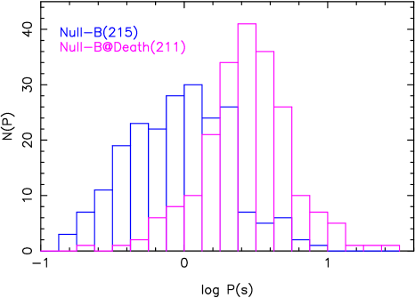
Figure 6: Distribution of P_s (blue) for NPSRs with available B_s values, marked as Null-B. The corresponding distribution of P_D (magenta) is marked as Null-B@Death. The number of objects for Null-B and Null-B@Death are different because four pulsars from the first group lie below death-line [2], used for calculating P_D.

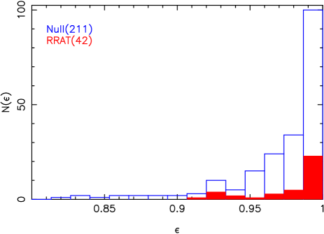
Figure 7: Distribution of $\epsilon$, as defined by Eq.(3), for the RRATs and the NPSRs. In both the cases, objects included in the distributions are those for which B_s values are known, and their current locations, in the P_s-B_s plane, are above death-line [2].

It is to be noted that P_D or $\tau_{D}$ and hence the proximity parameter, $\epsilon$, can only be calculated where the current value of $\dot{\rm P}_{s}$ has been measured. This is why such a calculation can be done only for a small number of RRATs, even though it is possible to obtain $\epsilon$ for almost the entire population of NPSRs. Moreover, for any given choice of death-line, there exist a few objects which fall on the right of the line (in the P_s-B_s) plane. This happens because every theoretical death-line makes certain simplifying assumptions which may or may not be applicable for a given pulsar. So, these ’beyond death-line’ pulsars have also been excluded from the $\epsilon$ calculation.

	PD	PKS(N)	DKS(N)	$\epsilon$
RRAT (42)	6.44s	0.93	0.08	0.96
NPSR (211)	3.52s	0.57	0.05	0.96
ALL (253)	4.01s	0.61	0.05	0.96
KS2(R-N)	PD	PD	$\epsilon$	$\epsilon$
	PKS	DKS	PKS	DKS
	$<10^{-3}$	0.36	0.90	0.09

Table 3: The average values of P_D and $\epsilon$ (see text for the definitions) for the RRAT, the NPSR and the combined populations. Kolmogorov-Smirnov test statistics, P_KS(N) and D_KS(N), to check whether P_D is normally distributed. (This test is nor performed on $\epsilon$ as it is clearly an asymmetric, skewed distribution.) P_KS(R-N) & D_KS(R-N) are the corresponding quantities for the null hypothesis that both the RRATs and the NPSRs are drawn from the same underlying population. Data : a) RRAT - Appendix A, b) NPSR - NULL Catalogue.

The average values of P_D and $\dot{\rm P}$_D are shown in Table-[3]. For the NPSRs, it can be seen from Fig.6 that P_D has a very clear log-normal distribution with the peak at $\sim 2.5s$. Though it is not as obvious for the RRATs, the P_D distribution is again nearly log-normal albeit with a higher peak value of $\sim 5s$. Surprisingly, contrary to expectation, the proximity parameter for both the RRATs and the NPSRs have rather similar behaviour. Even though close to the death-line, both types of objects have larger fractions of their life-time to go through yet. This likely rules out the possibility that nulling or RRAT behaviour can be treated simply as an ‘old age’ characteristic appearing in a particular evolutionary phase. However, as mentioned above, such a conclusion crucially depends on the assumption of constant surface magnetic fields which may or may not be true for the objects under consideration.

Therefore, it is important to consider other evolutionary connections for the RRATs. In the next section we discuss a few important conjectures of that nature.

5 Other Connections

RRAT	Ps	Bs	DM	Other
J-Name	s	1012 G	pc.cm-3
J0828-3417	1.85	1.37	52.20	RPSR
J0941-39	0.59	—-	78.20	NPSR
J1119-6127	0.41	41.00	704.80	RPSR
				Magnetar
J1647-3607	0.21	0.17	224.00	NPSR
J1819-1458	4.26	49.60	196.00	Magnetar
J1840-1419	6.60	6.55	19.40	NPSR
J1854-1557	3.45	4.00	150.00	NPSR
J1913+1330	0.92	2.86	175.64	NPSR
J2033+0042	5.01	7.05	37.84	NPSR

Table 4: RRATs that also occasionally show up as other kinds of neutron stars (indicated in the last column). Here, RPSR means radio pulsars not known to show any nulling behaviour.

Initially, the RRAT phenomenon was considered to be a manifestation of certain selection bias and / or the sensitivity of a telescope. For example, they were thought to be giant pulses from weak pulsars [Knight et al. (2006)]; or to be pulsars, with special emission behaviour, being far away (as discussed in §3). But there appears to be far more to the RRATs than simple observational effects.

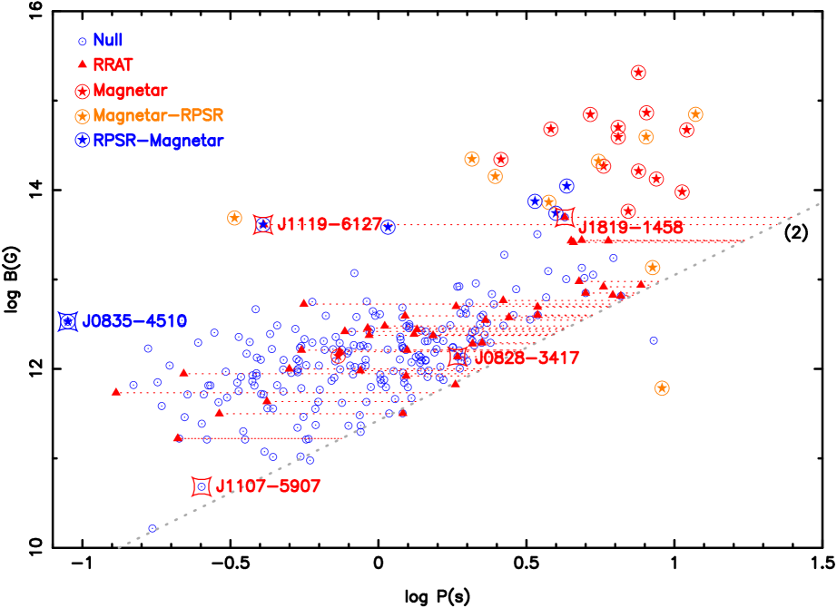
Figure 8: Distribution of RRATs (red triangles), NPSRs (circled dot in blue) and Magnetars (circled stars in orange) in the P_s–B_s plane. Green circled stars represent either a Magnetars exhibiting RPSR characteristics or an RPSRs exhibiting Magnetar characteristics. The red dashed-lines are evolutionary tracks of RRATs to the theoretical death-line ‘(2)’ (grey dashed-line), with constant B_s. See text for the significance of the named pulsars. Data : a) RRAT - Appendix A, b) NPSR - NULL Catalogue, c) Magnetar - Magnetar Catalog (http://www.physics.mcgill.ca/ pulsar/magnetar/main.html).

Besides the NPSRs, regular non-nulling RPSRs have also been observed to behave like RRATs, like J0828-3417 or J1119-6127. While J0828-3417 is an ordinary pulsar with a low DM, J1119-6127 is a high-magnetic field pulsar with a rather high value of DM (see Table-[4]). In fact, J1119-6127 has been observed to exhibit different types of radio behaviour at different epochs, with RRAT-like events typically preceded by large spin-period glitches. ?) argued that the glitches could be responsible for reconfiguration of the magnetic field giving rise to such changed emission behaviour, and that this likely indicates the existence of a group of neutron stars that become visible for a brief while only in the immediate aftermath of glitch activity.

It has also been suggested that RRATs likely have evolutionary links with the Magnetars [McLaughlin et al. (2009)] or the XDINS [Popov et al. (2006)]. Observation of RRATs in X-ray would help confirming such links. Unfortunately, only two RRATs, J1819-1458 [McLaughlin et al. (2007)] and J1119-6127 [Archibald et al. (2017)], have been observed in X-rays with upper limits for the X-ray luminosity estimated for another two RRATs (J0847-4316, J1846-0257). Most probably, the main reason for X-ray non-detection of RRATs is the uncertainties in source positions [Kaplan et al. (2009)]. The post-glitch recovery of the frequency derivatives (decrease in the average spin-down rate instead of an increase), as well as the X-ray outbursts of J1819-1458 and J1119-6127 have been observed to be clearly Magnetar-like [Lyne et al. (2009), Rea et al. (2010), Archibald et al. (2017), Bhattacharyya et al. (2018)]. Given the unusual change in $\dot{\rm P}_{s}$, it has been suggested that J1819-1458 is actually transitioning from being a Magnetar to an RRAT [Lyne et al. (2009)]. The view that the RRATs could be an evolutionary stage rather than a separate class of neutron stars is indeed strengthened by such observations.

On the other hand, ?) has argued for a case of accretion-induced revival of a pulsar, that has evolved beyond the death-line, in their fallback-disc model to explain the behaviour of J1819-1458. This model, while reproducing the observed values of P_s, $\dot{\rm P}_{s}$ and the X-ray luminosity, obtains a dipolar field strength of $\sim 5\times 10^{11}$ G at the polar cap. This value of the magnetic field combined with the measured P_s implies a ‘dead’ pulsar, located beyond the death-line in the P_s–B_s plane. If this indeed is the case, then only accretion can explain the X-ray activity. It is therefore argued that J1819-1458 is evolving towards becoming an XDINS, reinforcing an earlier suggestion of the connection between RRATs with such objects. One needs to remember that the magnetic field obtained in this model is much smaller than the field inferred from the dipole torque formula (quoted in Table-[4]). However, an absorption line at $\sim$ 1 keV has been detected in the X-ray spectrum of J1819-1458 [Rea et al. (2009)]. If this happens to be a cyclotron absorption line, then the required field strengths would be $2\times 10^{14}$ G and $\sim 10^{11}$ G for protons and electrons respectively [Miller et al. (2013)].

It is also interesting to consider J1107-5907, which arguably could have appeared to be an RRAT had it been located at a larger distance, in the light of this suggestion. It is is an old, isolated radio pulsar and in the P_s-B_s plane located in the region between those of normal and recycled pulsars. There exists a possibility that such pulsars are mildly recycled in high-mass X-ray binaries (HMXB) [Konar & Bhattacharya (1999), Konar (2017)]. If so, then RRAT phenomenon could indeed be related to accretion-induced changes in the magnetic field structure.

Fig.8 shows the possible import of the connections discussed above. Not only RRATs and NPSRs, but Magnetars along-with RPSRs exhibiting Magnetar characteristics have been shown here. Clearly high-magnetic field RRATs inhabit the same region of the P_s-B_s space as the Magnetars. Now, Magnetars are understood to be powered by the decay of their magnetic fields. Considering the relative locations, it is quite conceivable that the Magnetars may end up as RRATs in the course of their evolution.

J1107-5907, J0828-3417, J1119-6127 and J1819-1458 have been individually marked in Fig.8 to highlight their special characteristics. It is seen that J1107-5907, an NPSR and likely to have RRAT-like behaviour if located at a larger distance, is somewhat far away from both the majority of RRATs as well as NPSRs. Though, we must remember that only about 25% of the known RRATs are seen in this diagram as the rest do not have a B_s estimate. On the other hand, J0828-3417, a similar object, sits right in the middle of the NPSR as well as the RRAT population. Of the two Magnetar-like objects, while J1819-1458 is in the Magnetar region, J1119-6127 is quite far away from all three (RRAT, NPSR, Magnetar) groups. One possibility is that these objects (J1107-5907, J1119-6127) really are the missing links, transitioning from one class to another and are caught at the regions of transition. Another interesting object is J0835-4510, also shown in Fig.8, is a known NPSR which sometimes show Magnetar-like behaviour. These objects clearly demonstrate the intertwining connections between many distinct observational classes of neutron stars.

We have also shown the trajectories of RRATs, from their present location to the death-line, in Fig.8 assuming a constant surface dipolar magnetic field. It is obvious from these tracks that, unless they are intrinsically different, the RRATs and the NPSRs would be part of the same underlying population. In §3 we have noted that they are not. Therefore, it is likely that the assumption of an RRAT having a constant magnetic field is incorrect, even it is true for regular RPSRs inclusive of the NPSRs [Bhattacharya et al. (1992), Konar & Bhattacharya (1997)].

Random, sporadic processes have also been considered to explain the RRAT phenomenon. For example, the quasi-periodic activity of B1931+24 (J1933+2421) has been thought to arise from the interactions between the neutron star magnetosphere and the precessing debris disk surrounding it [Li (2006)], or because of the migration of asteroids (formed from supernova fallback material) into pulsar light-cylinder region disrupting the emission process [Cordes & Shannon (2008)]. It has also been suggested that pulsars can have radiation belts, similar to those in planetary magnetosphere, and sporadic release of plasma trapped therein can interfere with pulsar emission processes giving rise to RRAT-like behaviour [Luo & Melrose (2007)]. Moreover, some of the single pulse events initially thought to be RRATs have now been tagged as potentially mislabeled FRBs [Keane (2016)]. Quite Clearly, even if such explanations hold good for certain specific RRATs, the majority of objects demand a more general scenario.

6 Conclusions

The RRATs, one of the latest observational sub-classes, comprise a tiny ($<5\%$) subset of the known neutron stars. As yet, there is no clear understanding of the nature of their sporadic emission. In this work, we have considered the population of RRATs and discussed some of the prominent hypotheses (offered to explain the RRAT phenomenon) in the light of the general properties of this population.

First of all, considering the population characteristics, we come to the conclusion that the RRAT behaviour can neither be explained as special observational effects or as a result of certain random processes.

One of the main trains of thought, regarding the RRATs has been about their connection with the NPSRs. Comparing the two populations, we find that -

• The RRATS are bounded by death-line [2], like the NPSRs.

• RRATs have, on the average, higher P_s and B_s than NPSRs.

• RRATs tend to have smaller DM compared to the NPSRs.

• P_s & B_s of RRATs and NPSRs as well as the combined population appear to have log-normal distribution.

• The statistical distributions of P_s, B_s and DM for RRATs and NPSRs do not appear to come from the same underlying distribution.

Thus, we conclude that the RRATs and the NPSRs, even if connected through evolution, do not come directly from the same underlying population, and RRAT behaviour is unlikely to be a manifestation of extreme nulling.

Another important conjecture has been to attribute the RRAT behaviour to the proximity of these neutron stars to the death-line. We have considered this assertion by quantifying the death-line nearness through the proximity parameter, $\epsilon$. We find that the RRATs appear to have a significant part of their active life left before they would reach the death-line. Even though this finding crucially depends on the assumption of a constant magnetic field, if true this indicates that the RRAT behaviour is not a direct consequence of old age.

However, we find two very different and intriguing conjectures to hold some promise. First, the RRAT phenomenon could be associated with re-structuring of magnetic fields. This could either be accretion-induced, through the revival of ‘dead’ pulsars. Or it could be glitch-induced. Second, the RRATs could be later evolutionary stages of other varieties of neutron stars like the Magnetars [Konar (2012)]. Even though a recent work suggests that the Magnetars are likely to evolve into XDINS [Jawor & Tauris (2022)], in an independent work [Chowhan et al. (2022)] we find that even though majority of the Magnetars are likely to evolve into XDINS, some of the Magnetars as well as most of the high magnetic radio pulsars are likely to evolve into RRATs.

7 Acknowledgment

We thank Priya S Hasan & S N Hasan whose 2020 workshop, on “Astronomy from Archival Data" as part of an IAU-OAD project, helped bring the authors of this work together.

Appendix A The RRATs

The following tables list the known RRATs, detected till date, that we have used for our calculations in this work. Majority of the sources are obtained from the RRATalog site maintained by Bingyi Cui and Maura McLaughlin. For the rest, discovery papers have been referred to. The parameter values for spin period (P_s), dispersion measure (DM), characteristic age ($\tau_{c}$) and surface dipolar field (B_s) are taken from the ATNF Pulsar Catalogue [Manchester et al. (2005)], except where the objects are not yet included in the ATNF list. Parameter values for these second set of objects are taken from the discovery papers and the references are marked with a ‘-P’. For some sources, different names have been used by different groups. We have primarily used the ATNF names and indicated the alternative names in the ‘Other-Name’ column. The references cited in the tables with numbers ranging from 1 to 8 correspond to the following.

(1) - RRATalog (last update September, 2016);

(2) - ?);

(3) - ?);

(4) - ?);

(5) - ?);

(6) - ?);

(7) - ?);

(8) - ?);

(9) - ?).

RRATalog : http://astro.phys.wvu.edu/rratalog/

ATNF : http://www.atnf.csiro.au/research/pulsar/psrcat/

Table 5: List of RRATs

	B-Name	J-Name	Other-Name	Ps	DM	$\tau$	Bs
				s	Pfc.cm-3	yr	G
001	J0054+66	J0054+66		1.39	15.00			(1)
002	J0054+69	J0054+69			90.30			(1)
003	J0103+54	J0103+54		0.35	55.60			(1)
004	J0121+53	J0121+53		2.72	91.38			(7)
005	J0139+3336	J0139+3336		1.25	21.23	9.58e+06	1.62e+12	(6)
006	J0156+04	J0156+04			27.50			(1)
007	J0318+1341	J0318+1341		1.97	12.05			(1-P)
008	J0201+7005	J0201+7005		1.35	21.03	3.88e+06	2.76e+12	(1)
009	J0302+2252	J0302+2252	J0301+20	1.21	18.99	2.32e+08	3.19e+11	(1)
010	J0305+4001	J0305+4001			24.00			(6)
011	J0332+79	J0332+79		2.06	16.67			(1)
012	J0410-31	J0410-31		1.88	9.20			(1)
013	J0441-04	J0441-04			20.00			(1)
014	J0447-04	J0447-04		2.19	29.83			(1)
015	J0452+1651	J0452+1651			19.00			(6)
016	J0513-04	J0513-04			18.50			(1)
017	J0534+34	J0534+34	J0534+3407		24.50			(6)
018	J0544+20	J0544+20	J0544-20		56.90			(1)
019	J0545-03	J0545-03		1.07	67.20			(1)
020	J0550+09	J0550+09		1.75	86.60			(1)
021	J0609+1635	J0609+1635			85.00			(6)
022	J0614-03	J0614-03		0.14	17.90			(1-P)
023	J0621-55	J0621-55			22.00			(1)
024	J0625+1730	J0625+1730			58.00			(6)
025	J0627+16	J0627+16		2.18	113.00			(1)
026	J0628+0909	J0628+0909	J0628+09	1.24	88.30	3.59e+07	8.35e+11	(1)
027	J0640+0744	J0640+0744	J0641+07		52.00			(6)
028	J0736-6304	J0736-6304	J0735-62	4.86	19.40	5.07e+05	2.75e+13	(1,5-P)
029	J0803+34	J0803+34	J0803+3410		34.00			(5)
030	J0812+8626	J0812+8626			40.25			(9)
031	B0826-34	J0828-3417		1.85	52.20	2.94e+07	1.37e+12	(3)
032	J0837-24	J0837-24			142.80			(1)
033	J0845-36	J0845-36		0.21	29.00	2.61e+07	1.67e+11	(1-P)
034	J0847-4316	J0847-4316		5.98	292.50	7.90e+05	2.71e+13	(1)
035	J0912-3851	J0912-3851	J0912-38	1.53	71.50	6.74e+06	2.37e+12	(1)
036	J0923-31	J0923-31			72.00			(1)
037	J0941+1621	J0941+1621			23.00			(6)
038	J0941-39	J0941-39		0.59	78.20			(1)
039	J0957-06	J0957-06		1.72	26.95			(1)
040	J1005+30	J1005+30			17.50			(6)
041	J1010+15	J1010+15			42.00			(4)
042	J1014-48	J1014-48		1.51	87.00			(1)
043	J1048-5838	J1048-5838		1.23	70.70	1.60e+06	3.92e+12	(1)
044	J1059-01	J1059-01			18.70			(1)
045	J1111-55	J1111-55			235.00			(1)
046	J1119-6127	J1119-6127		0.41	704.80	1.61e+03	4.10e+13	(2)
047	J1126-27	J1126-27		0.36	26.86			(1)
048	J1129-53	J1129-53		1.06	77.00			(1)
049	J1132+0921	J1132+0921			22.00			(6)
050	J1132+25	J1132+25	J1132+2515	1.00	23.00			(6)

Table 6: List of RRATs - continued.

	B-Name	J-Name	Other-Name	Ps	DM	$\tau$	Bs
				s	PVC.cm-3	yr	G
051	J1135-49	J1135-49			114.00			(1)
052	J1153-21	J1153-21		2.34	34.80			(1)
053	J1216-50	J1216-50		6.35	110.00			(1)
054	J1226-3223	J1226-3223		6.19	36.70	1.39e+07	6.69e+12	(1)
055	J1252+53	J1252+53		0.22	20.70			(7)
056	J1307-67	J1307-67	J1308-67	3.65	44.00			(1)
057	J1311-59	J1311-59			152.00			(1)
058	J1317-5759	J1317-5759		2.64	145.30	3.33e+06	5.83e+12	(1)
059	J1326+33	J1326+33		0.04	4.00			(6)
060	J1329+13	J1329+13	J1329+1349		12.00			(6)
061	J1332-03	J1332-03		1.11	27.10			(1)
062	J1336-20	J1336-20		0.18	19.30			(1-P)
063	J1336+33	J1336+33	J1336+3346	3.01	8.50			(6)
064	J1346+0622	J1346+0622			8.00			(6)
065	J1354+24	J1354+24			20.00			(1)
066	J1400+21	J1400+21	J1400+2127		10.50			(6)
067	J1404+1210	J1404+1210		2.65	17.05			(6-P)
068	J1404-58	J1404-58			229.00			(1)
069	J1424-56	J1424-56	J1423-56	1.43	32.90			(1)
070	J1433+00	J1433+00			23.50			(1)
071	J1439+76	J1439+76		0.95	22.29			(1)
072	J1444-6026	J1444-6026		4.76	367.70	4.07e+06	9.51e+12	(1)
073	J1502+28	J1502+28	J1502+2813	3.78	14.00			(6)
074	J1513-5946	J1513-5946		1.05	171.70	1.94e+06	3.02e+12	(1)
075	J1534-46	J1534-46		0.36	64.40			(1)
076	J1538+2345	J1538+2345		3.45	14.91	7.93e+06	4.93e+12	(1)
077	J1541-42	J1541-42			60.00			(1)
078	J1549-57	J1549-57		0.74	17.70			(1)
079	J1550+0943	J1550+0943			21.00			(8)
080	J1554+18	J1554+18			24.00			(1)
081	J1554-5209	J1554-5209		0.13	130.80	8.65e+05	5.42e+11	(1)
082	J1555+01	J1555+01	J1555+0108		18.50			(6)
083	J1603+18	J1603+18		0.50	29.70			(1)
084	J1610-17	J1610-17		1.30	52.50			(1-P)
085	J1611-01	J1611-01		1.30	27.21			(1)
086	J1623-0841	J1623-0841	J1623-08	0.50	59.79	4.08e+06	1.00e+12	(1)
087	J1647-3607	J1647-3607	J1647-36	0.21	224.00	2.61e+07	1.67e+11	(1)
088	J1649-4653	J1649-4653	J1649-46	0.56	331.00	1.78e+05	5.32e+12	(1)
089	J1652-4406	J1652-4406		7.71	786.00	1.29e+07	8.66e+12	(1)
090	J1654-23	J1654-23	J1653-2330	0.55	74.50	6.31e+05	1.62e+12	(1-P)
091	J1703-38	J1703-38		6.44	375.00			(1)
092	J1705-04	J1705-04		0.24	42.95			(1)
093	J1707-4417	J1707-4417	J1704-44	5.76	380.00	7.84e+06	8.29e+12	(1)
094	J1709-43	J1709-43			228.00			(1)
095	J1717+03	J1717+03		3.90	25.60			(1)
096	J1720+00	J1720+00		3.36	46.20			(1)
097	J1724-35	J1724-35		1.42	554.90			(1)
098	J1727-29	J1727-29			93.00			(1)
099	J1732+2700	J1732+2700			36.50			(6)
100	J1739-2521	J1739-2521	J1739-25	1.82	186.40	1.20e+08	6.69e+11	(1)

Table 7: List of RRATs - continued.

	B-Name	J-Name	Other-Name	Ps	DM	$\tau$	Bs
				s	PRC.cm-3	yr	G
101	J1753-12	J1753-12		0.40	73.20			(1)
102	J1753-38	J1753-38		0.67	168.00			(1)
103	J1754-3014	J1754-3014	J1754-30	1.32	89.70	4.72e+06	2.45e+12	(1)
104	J1807-2557	J1807-2557	J1807-25	2.76	385.00	8.77e+06	3.76e+12	(1)
105	J1819-1458	J1819-1458		4.26	196.00	1.20e+05	4.96e+13	(1)
106	J1825-33	J1825-33		1.27	43.20			(1)
107	J1826-1419	J1826-1419		0.77	160.00	1.39e+06	2.63e+12	(1)
108	J1838+50	J1838+50		2.58	21.81			(7)
109	J1839-0141	J1839-0141	J1839-01	0.93	293.20	2.49e+06	2.38e+12	(1)
110	J1840-1419	J1840-1419		6.59	19.40	1.65e+07	6.55e+12	(1)
111	J1841-04	J1841-04	J1841-0448		29.00			(6)
112	J1843+01	J1843+01		1.27	251.90			(1)
113	J1846-0257	J1846-0257		4.48	237.00	4.42e+05	2.71e+13	(1)
114	J1848-1243	J1848-1243	J1842-12	0.42	91.96	1.49e+07	4.32e+11	(1)
115	J1848+1516	J1848+1516	J1849+15	2.24	77.44	2.11e+07	1.96e+12	(1)
			J1848+1518		75.00			(6)
116	J1849+0112	J1849+0112		1.83	217.20	1.59e+06	5.01e+12	(1-P)
117	J1850+15	J1850+15		1.38	24.70			(1)
118	J1853+04	J1853+04		1.32	549.30			(1)
119	J1854+0306	J1854+0306		4.56	192.40	4.98e+05	2.60e+13	(1)
120	J1854-1557	J1854-1557		3.45	150.00	1.21e+07	4.00e+12	(1)
121	J1856+09	J1856+09		2.17	193.40			(1)
122	J1859+07	J1859+07			303.00			(1)
123	J1901+11	J1901+11		0.41	268.90			(1)
124	J1905+0414	J1905+0414			383.00			(1)
125	J1905+0902	J1905+0902	J1905+09	0.22	433.40	9.88e+05	8.84e+11	(1)
126	J1906+03	J1906+03		1.26	212.00			(1-P)
127	J1909+0641	J1909+0641	J1909+06	0.74	36.70	3.65e+06	1.56e+12	(1)
128	J1911+00	J1911+00		6.94	100.00			(1)
129	J1912+08	J1912+08			96.00			(1)
130	J1913+1330	J1913+1330		0.92	175.64	1.69e+06	2.86e+12	(1)
131	J1915+06	J1915+06		0.64	214.50			(1)
132	J1915-11	J1915-11		2.18	91.06			(1)
133	J1917+11	J1917+11		5.06	319.00			(6-P)
134	J1917+1723	J1917+1723			38.00			(6)
135	J1919+1745	J1919+1745	J1919+17	2.08	142.30	1.93e+07	1.91e+12	(1)
136	J1925-16	J1925-16		3.89	88.00			(1)
137	J1927+1725	J1927+1725	J1928+17	0.29	136.00	1.26e+07	3.16e+11	(1-P)
138	J1928+15	J1928+15		0.40	242.00			(1)
139	J1929+11	J1929+11		3.22	80.00			(1-P)
140	J1930+0104	J1930+0104			42.00			(6)
141	J1931+42	J1931+42			50.90			(7)
142	J1944-10	J1944-10		0.41	31.01			(1)
143	J1946+24	J1946+24		4.73	96.00			(1)
144	J1952+30	J1952+30		1.67	188.60			(1)
145	J1956-28	J1956-28		0.26	45.69			(1)
146	J1958+30	J1958+30		1.10	199.30			(1)
147	J2000+29	J2000+29		3.07	132.50			(1)
148	J2007+20	J2007+20		4.63	67.00			(1)
149	J2033+0042	J2033+0042	J2033+00	5.01	37.84	8.20e+06	7.05e+12	(1)
150	J2047+1259	J2047+1259			36.00			(8)

Table 8: List of RRATs - continued.

	B-Name	J-Name	Other-Name	Ps	DM	$\tau$	Bs
				s	pc.cm-3	yr	G
151	J2052+1308	J2052+1308			42.00			(6)
152	J2105+19	J2105+19	J2105+1917		33.00			(6)
153	J2105+6223	J2105+6223		2.30	50.75	7.00e+06	3.51e+12	(1)
154	J2107+2606	J2107+2606			10.50			(6)
155	J2135+3032	J2135+3032			63.00			(6)
156	J2146+2148	J2146+2148			43.00			(6)
157	J2202+21	J2202+21	J2202+2147		17.00			(6)
158	J2205+2244	J2205+2244			22.00			(6)
159	J2210+2118	J2210+2118			45.00			(6)
160	J2225+35	J2225+35		0.94	51.80			(1)
161	J2311+67	J2311+67		1.94	97.10			(1-P)
162	J2325-0530	J2325-0530		0.87	14.97	1.34e+07	9.57e+11	(1)

References

- Archibald et al. (2017) Archibald R. F. et al., 2017, ApJ, 849, L20
- Backer (1970) Backer D. C., 1970, Nature, 228, 42
- Bhattacharya et al. (1992) Bhattacharya D., Wijers R. A. M. J., Hartman J. W., Verbunt F., 1992, A&A, 254, 198
- Bhattacharyya et al. (2018) Bhattacharyya B. et al., 2018, MNRAS, 477, 4090
- Burke-Spolaor & Bailes (2010) Burke-Spolaor S., Bailes M., 2010, MNRAS, 402, 855
- Burke-Spolaor et al. (2011) Burke-Spolaor S. et al., 2011, MNRAS, 416, 2465
- Burke-Spolaor et al. (2012) Burke-Spolaor S. et al., 2012, MNRAS, 423, 1351
- Chen & Ruderman (1993) Chen K., Ruderman M., 1993, ApJ, 402, 264
- Chowhan et al. (2022) Chowhan T. T., Konar S., Banik S., 2022, in Troja E., Baring M., ed, Neutron Star Astrophysics at the Crossroads: Magnetars and the Multimessenger Revolution, Proceedings of IAU Symposium No. 363 (in press), arXiv:2201.05248
- Cordes & Shannon (2008) Cordes J. M., Shannon R. M., 2008, ApJ, 682, 1152
- Cui et al. (2017) Cui B. Y., Boyles J., McLaughlin M. A., Palliyaguru N., 2017, ApJ, 840, 5
- Deneva et al. (2013) Deneva J. S., Stovall K., McLaughlin M. A., Bates S. D., Freire P. C. C., Martinez J. G., Jenet F., Bagchi M., 2013, ApJ, 775, 51
- Esamdin et al. (2012) Esamdin A., Abdurixit D., Manchester R. N., Niu H. B., 2012, ApJ, 759, L3
- Gençali & Ertan (2018) Gençali A. A., Ertan Ü., 2018, MNRAS, 481, 244
- Good et al. (2021) Good D. C. et al., 2021, ApJ, 922, 43
- Hessels et al. (2008) Hessels J. W. T., Ransom S. M., Kaspi V. M., Roberts M. S. E., Champion D. J., Stappers B. W., 2008, in American Institute of Physics Conference Series, Vol. 983, Bassa C., Wang Z., Cumming A., Kaspi V. M., ed, 40 Years of Pulsars: Millisecond Pulsars, Magnetars and More, p. 613
- Hewish et al. (1968) Hewish A., Bell S. J., Pilkington J. D. H., Scott P. F., Collins R. A., 1968, Nature, 217, 709
- Jawor & Tauris (2022) Jawor J. A., Tauris T. M., 2022, MNRAS, 509, 634
- Kaplan et al. (2009) Kaplan D. L., Esposito P., Chatterjee S., Possenti A., McLaughlin M. A., Camilo F., Chakrabarty D., Slane P. O., 2009, MNRAS, 400, 1445
- Kaspi (2010) Kaspi V. M., 2010, Proceedings of the National Academy of Science, 107, 7147
- Keane (2016) Keane E. F., 2016, MNRAS, 459, 1360
- Keane & Kramer (2008) Keane E. F., Kramer M., 2008, MNRAS, 391, 2009
- Keane et al. (2011) Keane E. F., Kramer M., Lyne A. G., Stappers B. W., McLaughlin M. A., 2011, MNRAS, 415, 3065
- Keane et al. (2010) Keane E. F., Ludovici D. A., Eatough R. P., Kramer M., Lyne A. G., McLaughlin M. A., Stappers B. W., 2010, MNRAS, 401, 1057
- Keane & McLaughlin (2011) Keane E. F., McLaughlin M. A., 2011, Bulletin of the Astronomical Society of India, 39, 333
- Knight et al. (2006) Knight H. S., Bailes M., Manchester R. N., Ord S. M., Jacoby B. A., 2006, ApJ, 640, 941
- Konar (2012) Konar S., 2012, in COSPAR Meeting, Vol. 39, 39th COSPAR Scientific Assembly, p. 961
- Konar (2013) Konar S., 2013, in Astronomical Society of India Conference Series, Vol. 8, Das S., Nandi A., Chattopadhyay I., ed, Astronomical Society of India Conference Series, p. 89
- Konar (2017) Konar S., 2017, Journal of Astrophysics and Astronomy, 38, 47
- Konar et al. (2016) Konar S. et al., 2016, Journal of Astrophysics and Astronomy, 37, 36
- Konar & Bhattacharya (1997) Konar S., Bhattacharya D., 1997, MNRAS, 284, 311
- Konar & Bhattacharya (1999) Konar S., Bhattacharya D., 1999, MNRAS, 303, 588
- Konar & Deka (2019) Konar S., Deka U., 2019, Journal of Astrophysics and Astronomy, 40, 42
- Li (2006) Li X.-D., 2006, ApJ, 646, L139
- Logvinenko et al. (2020) Logvinenko S. V., Tyul’bashev S. A., Malofeev V. M., 2020, Bulletin of the Lebedev Physics Institute, 47, 390
- Lu et al. (2019) Lu J. et al., 2019, Science China Physics, Mechanics, and Astronomy, 62, 959503
- Luo & Melrose (2007) Luo Q., Melrose D., 2007, MNRAS, 378, 1481
- Lyne et al. (2009) Lyne A. G., McLaughlin M. A., Keane E. F., Kramer M., Espinoza C. M., Stappers B. W., Palliyaguru N. T., Miller J., 2009, MNRAS, 400, 1439
- Manchester et al. (2005) Manchester R. N., Hobbs G. B., Teoh A., Hobbs M., 2005, VizieR Online Data Catalog, 7245, 0
- McLaughlin et al. (2009) McLaughlin M. A. et al., 2009, MNRAS, 400, 1431
- McLaughlin et al. (2006) McLaughlin M. A. et al., 2006, Nature, 439, 817
- McLaughlin et al. (2007) McLaughlin M. A. et al., 2007, ApJ, 670, 1307
- Miller et al. (2013) Miller J. J., McLaughlin M. A., Rea N., Lazaridis K., Keane E. F., Kramer M., Lyne A., 2013, ApJ, 776, 104
- Popov et al. (2006) Popov S. B., Turolla R., Possenti A., 2006, MNRAS, 369, L23
- Rea et al. (2010) Rea N. et al., 2010, MNRAS, 407, 1887
- Rea et al. (2009) Rea N. et al., 2009, ApJ, 703, L41
- Ritchings (1976) Ritchings R. T., 1976, MNRAS, 176, 249
- Ruderman & Sutherland (1975) Ruderman M. A., Sutherland P. G., 1975, ApJ, 196, 51
- Shitov et al. (2009) Shitov Y. P., Kuzmin A. D., Dumskii D. V., Losovsky B. Y., 2009, Astronomy Reports, 53, 561
- Tyul’bashev et al. (2021) Tyul’bashev S., Kitaeva M., Logvinenko S., G.E. T., 2021, Astronomy Reports (in press)
- Tyul’bashev et al. (2018) Tyul’bashev S. A., Tyul’bashev V. S., Malofeev V. M., 2018, A&A, 618, A70
- von Mises (1980) von Mises R., 1980, Mathematical Theory of Probability and Statistics. Academic Press, New York
- Weltevrede et al. (2011) Weltevrede P., Johnston S., Espinoza C. M., 2011, MNRAS, 411, 1917
- Weltevrede et al. (2006) Weltevrede P., Stappers B. W., Rankin J. M., Wright G. A. E., 2006, ApJ, 645, L149
- Young et al. (2014) Young N. J., Weltevrede P., Stappers B. W., Lyne A. G., Kramer M., 2014, MNRAS, 442, 2519