Machine Learning Approach to the Floquet–Lindbladian Problem

Abstract

Similar to its classical version, quantum Markovian evolution can be either time-discrete or time-continuous. Discrete quantum Markovian evolution is usually modeled with completely-positive trace-preserving maps while time-continuous evolution is often specified with superoperators referred to as "Lindbladians". Here we address the following question: Being given a quantum map, can we find a Lindbladian which generates an evolution identical – when monitored at discrete instances of time – to the one induced by the map? It was demonstrated that the problem of getting the answer to this question can be reduced to an NP-complete (in the dimension $N$ of the Hilbert space the evolution takes place in) problem. We approach this question from a different perspective by considering a variety of Machine Learning (ML) methods and trying to estimate their potential ability to give the correct answer. Complimentary, we use the performance of different ML methods as a tool to check the hypothesis that the answer to the question is encoded in spectral properties of the so-called Choi matrix, which can be constructed from the given quantum map. As a test bed, we use two single-qubit models for which the answer can be obtained by using the reduction procedure. The outcome of our experiment is that, for a given map, the property of being generated by a time-independent Lindbladian is encoded both in the eigenvalues and the eigenstates of the corresponding Choi matrix.

The question posed in the abstract is a quantum version of the "embedding problem" formulated by Elfving in 1937 Elfving (1937) for classical Markov processes: Given map $\mathcal{P}$ can we find generator $\mathcal{L}$ such that $\mathcal{P}=\mathrm{exp}(\mathcal{L}T)$, where $T$ is the given time interval? Answer "yes" would mean that the original time-discrete evolution can be obtained from the constructed continuous-time evolution by monitoring the latter at the time instances $t=T,2T,...$. It may also be that the answer is "no" and the time-discrete evolution cannot be obtained as a stroboscopic sample of any time-continuous Markovian evolution.

The problem of finding the answer for a given completely positive trace-preserving (CPTP) map $\mathcal{P}$ was called "[quantum] Markovianity problem" Wolf et al. (2008). An algorithm to obtain the answer, based on a reduction of the original problem to a particular problem of integer semidefinite programming, has also been proposed Wolf et al. (2008). In its turn, this particular problem was shown Cubitt, Eisert, and Wolf (2012) to be reducible to the well-known NP-complete $\mathrm{1{\text{-}}IN{\text{-}}3{\text{-}}SAT}$ problem Garey and Johnson (1979). There is no surprise that the algorithm has an exponential complexity with respect to the problem dimension $N$. A recent attempt to implement the algorithm demonstrated that the practical horizon is limited by $N=8$ (e.g., by models consisting of no more than three spins/qubits) Volokitin et al. (2022).

Recently, the Markovianity problem has gained particular attention in the context of open quantum evolution governed by time-dependent Lindbladians. While the stroboscopic version of coherent quantum evolution, determined by a time-periodic Hamiltonian, can always be obtained with an effective time-independent Floquet Hamiltonian Holthaus (2015); Bukov, D’Alessio, and Polkovnikov (2015), it is no longer so in the case of open quantum evolution induced by a time-periodic Lindbladian, $\mathcal{L}(t)$, $\mathcal{L}(t+T)=\mathcal{L}(t)$ Schnell, Eckardt, and Denisov (2020). The reason for that is that a generator – if it is of the Lindblad form – has to fulfill some very specific properties. Currently, the problem of the existence of effective Floquet-Lindbladians is actively discussed in the literature Yusipov et al. (2021); Zhang (2016); Kramer (2013); Suykens and Vandewalle (1999); Amari and Wu (2001); Dagher (2008), and different expansion techniques are used to derive Floquet-Lindbladians. However, most of the illustrative results are limited by $N=2$.

One of the current trends in the quantum community is to address many-body systems. In the context of the Floquet-Lindbladian problem that means that it is important to step beyond single spin/qubit models. Here we approach the problem from a new perspective, by considering it as a generic optimization problem and trying to analyze it by using the toolbox of Machine Learning methods. Our motivation is that some of these methods may give us a chance to get beyond the limit set by the reduced problem.

I Introduction

We start right with the problem formulation and consider the time-dependent Markovian master equation Breuer (2004); Breuer, Laine, and Piilo (2009)

$$\dot{\rho}=\mathcal{L}(t)\rho=-\frac{i}{\hbar}[H(t),\rho]+\mathcal{D}(t)\rho,$$ (1)

governing density operator $\rho$ of the model system. The evolution is set by a time-periodic generator of the Gorini-Kossakowski-Sudarshan-Lindblad form (henceforth "Lindbladian") Gorini, Kossakowski, and Sudarshan (1976); Lindblad (1976), $\mathcal{L}(t)=\mathcal{L}(t+T)$. It is characterized by a time-periodic Hamiltonian $H(t)$ and the dissipative part

$$\mathcal{D}(t)\rho=\sum_{i}\gamma_{i}(t)\big{[}L_{i}(t)\rho L_{i}^{\dagger}(t)-\frac{1}{2}\{L_{i}^{\dagger}(t)L_{i}(t),\rho\}\big{]},$$ (2)

with jump operators $L_{i}(t)$ and non-negative rates $\gamma_{i}(t)$. In general, jump operators and rates are also time-periodic, with the same period $T$. Under these conditions it is guaranteed that, for any time $t$, the corresponding evolution can be reproduced with a completely positive (CP) and trace preserving (TP) map Breuer, Laine, and Piilo (2009),

$$\mathcal{P}(t)=\mathcal{T}\exp\left(\int_{0}^{t}\mathrm{d}t\mathcal{L}(t)\right).$$ (3)

where $\mathcal{T}$ is the standard time-ordering operator.

We will address the stroboscopic evolution set by the map

$$\mathcal{P}(T)=\mathcal{T}\exp\bigg{[}\int_{0}^{T}\!\mathrm{d}t\,\mathcal{L}(t)\bigg{]}.$$ (4)

The repeating action of this map induces the time-discrete evolution of the system, $\rho(0)$ we have $\rho(nT)=\mathcal{P}(T)^{n}\rho(0)$. We now define a Floquet generator as a time-independent superoperator $\mathcal{K}$, such that

$$\mathcal{P}(T)=\exp\left({\mathcal{K}T}\right)\quad\text{ or }\quad\mathcal{K}=\frac{\log(\mathcal{P})}{T}$$ (5)

for the open driven system described by Eq. (1). If the Floquet generator can be recast into the Lindblad form, i.e., in the form given by Eq. (1) but with all operators and rates time-independent, we call the corresponding Floquet generator Floquet-Lindbladian and write

$$\mathcal{L}_{F}=\mathcal{K}.$$ (6)

Now we pose the main question: Is there a Floquet-Lindbladian $\mathcal{L}_{F}$ for a given time-periodic Lindbladian $\mathcal{L}(t)$, $\mathcal{L}(t+T)=\mathcal{L}(t)$?

It was demonstrated Wolf et al. (2008); Cubitt, Eisert, and Wolf (2012) that the answer to another question "Is there a Lindbladian for the given completely positive trace-preserving (CPTP) map?" [which is the map $\mathcal{P}(T)$ in our case] can be obtained by reducing the original problem to an integer nonlinear programming problem. Therefore, formally, there is a way to get the answer to the question about the existence of Floquet-Lindbladian.

The number of variables $n$ in the reduced problem can be estimated straightforwardly. It is limited by the maximal possible number of complex conjugated pairs in the spectrum of the map Wolf et al. (2008); Cubitt, Eisert, and Wolf (2012), $n_{\mathrm{max}}=\lfloor\frac{N^{2}-1}{2}\rfloor$ (one is subtracted because at least one of the eigenvalues is equal to $1$). Here $N$ is the dimension of the Hilbert space $\mathcal{H}$ the map is acting in and $\lfloor...\rfloor$ is the floor operation, i.e., it gives the greatest integer less than or equal to the real input. For example, for $N=8$ we could have up to $n=31$ integer variables and the answer to the question is "yes" if there is at least one point of the lattice $\mathbb{Z}^{31}$ for which the set of the necessary (and altogether sufficient) conditions Wolf et al. (2008) is fulfilled.

It is indeed not possible to check all the points – even of $\mathbb{Z}^{1}$ – if the lattice is not limited. Luckily, a convex feasible region in the real space $\mathbf{R}^{n}$ can always be out-shaped Wolf et al. (2008). To prove that the answer is "yes" or "no", we have to check all integer points inside the feasible region (or use the Khachiyan-Porkolab algorithm Khachiyan and Porkolab (1997) instead). It was shown that this problem can be reduced to a well-known NP-complete – with respect to $n$ – problem Cubitt, Eisert, and Wolf (2012). That means that any practical algorithm based on this reduction will have an exponential complexity with respect to $n$.

The answer can be easily obtained for a one-qubit ($N=2$) model because in this case $n=1$ and the feasible region is just a finite interval Cubitt, Eisert, and Wolf (2012); Schnell, Eckardt, and Denisov (2020); Amari and Wu (2001). However, already for two-qubit models, the complete check of integer points inside a $7$-dimensional volume can take a substantial time. We implemented an algorithm Volokitin et al. (2022) that allowed us to out-shape the feasible volume and test it with several popular multi-spin models. It turned out that even in the case of three spins we have to deal with up to $10^{9}$ integer points for some, physically-relevant, values of model parameters. Even by taking into account the embarrassingly parallelizable character of the task (each point can be checked independently) and by running the algorithm on a medium-size cluster, one would need to wait for several hours before getting the answer Volokitin et al. (2022).

It is therefore doubtful that, by following this path, we would be able to get answers for four-qubit models in the general case, simply because it would not be possible to check all the integer points inside the feasible volume in the $127$-dimensional space. Yet here we need to recall that the algorithm we have used so far is based on a reduction of the original problem to a known NP-complete problem. Strictly speaking, the fact that one problem can be reduced to another, however, does not mean that both are equally complex. To speculate a bit further, many specific properties of the original matrices involved in the problem formulation were neglected in the course of the reduction so there is still a chance that the original problem, even though still belonging formally to the same NP-complete class, can be solved faster and with less computation resources Flum and Grohe (2006).

After realizing the complexity of the problem, it is very natural to think about alternatives, which could allow us to solve problems for a reasonable large number of qubits – at the expense of obtaining an answer which is not always correct but correct with some reasonably high accuracy. Here Machine Learning (ML) methods look like immediate candidates Carleo et al. (2019). We made the first step in this direction in Ref. Yusipov et al. (2021), where we tried to implement ML methods used for computer vision problems to reconstruct the boundary between ’yes/no’ region on the parameter plane of a two-qubit model. Unfortunately, the potential of this approach is rather limited as it requires extensive calculations on a coarse grid in the parameter plane for every new model and, therefore, is not capable of generalization. In addition, by training networks on images of ’yes/no’-boundaries we do not get closer to the understanding of mechanisms that determine the existence (or non-existence) of Floquet-Lindbladians.

In this paper, we use several ML algorithms and implement a parameterization which is based on specific properties of the operators and matrices related to the original problem. By using a one-qubit model, for which the correct answer can easily be obtained Wolf et al. (2008); Yusipov et al. (2021), we demonstrate that ML methods can "learn" the ’yes/no’-partition of the parameter space. We also discuss what methods and parameterizations give the best accuracy.

II Reduced problem

In order to be a Lindbladian, operator $\mathcal{K}$, Eq. (5), has to fulfilled two conditions. First, it has to preserve Hermiticty. In case $\mathcal{K}$ is a logarithm of a Floquet map, this is guaranteed since the map itself is Hermiticity preserving. Next, $\mathcal{K}$ has to be conditionally completely positive Wolf et al. (2008). Formally, this means that

$$\Phi_{\perp}\mathcal{K}^{\Gamma}\Phi_{\perp}\geq 0,$$ (7)

where $\Phi_{\perp}=\mathbf{1}-{\left|\Phi\right\rangle}{\left\langle\Phi\right|}$ is the projector on the orthogonal complement of the maximally entangled state ${\left|\Phi\right\rangle}=\sum_{i=1}^{N}\left({\left|i\right\rangle}\otimes{\left|i\right\rangle}\right)/\sqrt{N}$ with $\{{\left|i\right\rangle}\}$ denoting the canonical basis of ${\mathcal{H}}$.

A new object, $\mathbf{C}=\mathcal{K}^{\Gamma}=N(\mathcal{K}\otimes\mathbf{1})[{\left|\Phi\right\rangle}{\left\langle\Phi\right|}]$, is the Choi operator Choi (1975) corresponding to $\mathcal{K}$ which acts in the product Hilbert space $\mathcal{H}^{2}$. If $\mathcal{K}$ is given in the matrix form (by using some basis)

$$\widehat{\mathcal{K}}_{ij,kl}:=\langle i\otimes j|\mathcal{K}|k\otimes l\rangle.$$ (8)

the matrix form of the corresponding Choi operator is related to it by the reshuffling operation Życzkowski and Bengtsson (2004)

$$\mathbf{C}=\widehat{\mathcal{K}}^{\mathcal{R}},~{}~{}~{}\mathbf{C}_{ij,kl}=\widehat{\mathcal{K}}_{ik,jl}.$$ (9)

The reshuffling operation $\mathcal{R}$ is an involution so that being repeated twice it results in the identity transform. In the case when $\mathcal{K}$ is a CPTP map, the corresponding Choi operator is a state Choi (1975); Życzkowski and Bengtsson (2004), i.e., a density operator (though not normalized), in $\mathcal{H}^{2}$. For example, for any Floquet map $\mathcal{P}(T)$ we could get the corresponding state.

Condition (7) can be recast in some matrix inequality Wolf et al. (2008), if we use spectral decomposition of $\mathcal{K}$. Since the Floquet map is Hermiticty preserving, its spectrum is invariant under the complex conjugation. Therefore, the corresponding $N^{2}$ eigenvalues are either real or appear as complex conjugated pairs (strictly speaking, the spectrum could also include eigenvalues of odd degeneracy). We denote the numbers of real eigenvalues as $m$ and complex pairs as $n$. $\mathcal{P}(T)$ can be represented as

$$\mathcal{P}(T)=\sum_{r=1}^{m}\lambda_{r}P_{r}+\sum_{c=1}^{n}\left(\lambda_{c}P_{c}+\lambda_{c}^{*}P_{c*}\right),$$ (10)

where $\lambda_{r}$ are the real eigenvalues, $\{\lambda_{c},\lambda_{c}^{*}\}$ are the pairs of complex eigenvalues, and $P_{x}$ the corresponding projectors Wolf et al. (2008).

Any logarithmic branch, Eq. (5), of $\mathcal{P}(T)$ can be represented as

$$\mathcal{K}_{\{x_{1},...,x_{n}\}}=\mathcal{K}_{0}+i\omega\sum_{c=1}^{n}x_{c}\left(P_{c}-P_{c*}\right),$$ (11)

where $\mathcal{K}_{0}$ is the principle branch and $\omega=\frac{2\pi}{T}$. Therefore, every branch is parametrized with $n$ integers, $\{x_{1},...,x_{n}\}$, i.e., it corresponds to a vertex $\mathbf{x}=\{x_{1},...,x_{n}\}$ of the $\mathbb{Z}^{n}$ lattice. Now we introduce a set of operators (that are, in fact, Hermitian)

$$V_{0}=\Phi_{\perp}\mathcal{K}_{0}^{\Gamma}\Phi_{\perp},~{}~{}V_{c}=i\omega\Phi_{\perp}(P_{c}-P_{c}*)^{\Gamma}\Phi_{\perp},~{}~{}c=1,\dots,n.$$ (12)

and arrive at the following test Wolf et al. (2008):

Generator $\mathcal{K}_{\mathbf{x}}$ is Lindbladian iff there is a set of $n$ integers, $\mathbf{x}\in\mathbb{Z}^{n}$, such that $$V_{\mathbf{x}}=V_{0}+\sum_{c=1}^{n}x_{c}V_{c}\geq 0.$$ (13)

Such type of matrix inequalities (and related programming problems) is well known in the control theory; see. e.g., Ref. Boyd et al. (1994). The crucial difference is that in there vector $\mathbf{x}$ is considered to be real. If matrices $V_{c}$ are real and symmetric, the inequality out-shapes a convex feasible region known as spectrahedron Ramana and Goldman (1995). We deal with integers and this mere fact makes the problem NP-complete (with respect to the number of the matrices in the sum). However, we can benefit from the fact the feasible region (13) is convex if $\mathbf{x}\in\mathbb{R}^{n}$. That is, we can limit the number of integer points needed to be checked. This was implemented in the algorithm we discussed in the introduction.

Finally, imagine that we can quantify distance from ’Lindbladianity’ for any generator $\mathcal{K}_{\mathbf{x}}$. Then, if the answer is "no" and there is no such integer vector ${\mathbf{x}}$ that condition (13) holds (and, correspondingly, no Floquet-Lindbladian exists), we can define the distance from Markovianity for $\mathcal{P}(T)$ by picking the branch which gives the minimal distance. Such measure was proposed by Wolf et al. Wolf et al. (2008). It is based on adding a noise term $\mathcal{N}$, that is the generator of the depolarizing channel, $\exp(T\mu\mathcal{N})\rho=e^{-\mu T}\rho+[1-e^{-\mu T}]\frac{\mathbf{1}}{N}$, weighted with the strength $\mu$, to the generator and determining the minimal strength required to make at least one of the logarithmic branches Lindbladian , i.e.

$$\mu_{\mathrm{min}}=\inf\left\{\mu\geq 0{\Big{|}}\begin{array}[]{l}\mathcal{K}_{\mathbf{x}}+\mu\mathcal{N}\text{ is a valid}\\ \text{Lindblad generator}\end{array}\right\}.$$ (16)

III Methods

We select eleven popular ML methods implemented in the scikit-learn library Pedregosa et al. (2011). Namely, we use the k-nearest neighbors method (kNN) Zhang (2016); Kramer (2013), support vector machine (SVM) with linear, polynomial and RBF kernels Suykens and Vandewalle (1999); Dagher (2008), decision trees Safavian and Landgrebe (1991); Breiman et al. (1984), random forest (RF) Cutler, Cutler, and Stevens (2012); Breiman (2001), fully connected neural networks (FNN) Sanger (1989); Glorot and Bengio (2010), AdaBoost Freund and Schapire (1997), linear (LDA) and quadratic (QDA) discriminant analysis Fukunaga (2013), and naive Bayes classifiers Domingos and Pazzani (1997). All these methods are well described in the literature, so in this section we only explain the reasoning behind our choice.

The performance of kNN , decision trees, and random forest methods depends on how the elements of the training and test samples are distributed in the space. In all these methods, a direct comparison of an element from a test sample with a training sample and search for a similar element, are used. We could expect good performance of the methods in data interpolation if the training sample is representative, but the possibility of equally good extrapolation is questionable. Various implementations of SVM, discriminant analysis, and naive Bayes classifier have different features. Thus, we may expect to get reasonably accurate functional models of the boundaries between the ’yes’ and ’no’ regions.

The random forest, fully connected neural networks, and AdaBoost methods are able to build very complex models and highlight non-obvious features and can solve a complex problem in an accurate way. We are not only motivated by the idea to demonstrate the potential of ML methods in getting the answer for single-qubit models. In fact, we hope to get an intuitive understanding of how the specific mathematical nature of the problem influences the results of the classification. We expect that by analyzing the performance of these methods we can get an additional insight.

All the selected methods have a number of meta-parameters, some of which are set by default, while others are selected and optimized to get the best results. In particular, we vary the following parameters: the number of neighbors in kNN (typically 3-7), the degree of the kernel polynomial in the polynomial SVM (typically 2-11), the height of the decision tree (typically 3-15), the height (2-9) and the number (typically 50-300) of trees in random forest, the number of layers (typically 3-4) and their size (from 8 to 512) in fully connected neural networks, as well as the type of the AdaBoost classifiers (short decision trees) and the number of these classifiers (typically 50-300). In the following sections, we present only the best results obtained for each of the methods.

IV Model

As a test bed we used a single spin(qubit) model described with the following Hamiltonian Schnell, Eckardt, and Denisov (2020) (Problem I):

$$H(t)=\frac{\Delta}{2}\sigma_{z}+Ecos(\omega t+\varphi)\sigma_{x},~{}~{}L=\sigma\_$$ (17)

We also modified this model by adding one extra operator term to the Hamiltonian (Problem II):

$$H(t)=\frac{\Delta}{2}(\sigma_{z}+\sigma_{y})+Ecos(\omega t+\varphi)\sigma_{x},~{}~{}L=\sigma\_$$ (18)

For both models, we use the following parameter values: $\Delta=1,\gamma=0.01$. Such parameters as amplitude $E$, frequency $\omega$, and phase shift $\varphi$, are varied to generate data sets for the ML algorithms.

As it is shown in the previous section, solution of the Floquet-Lindbladian existence problem reduces to the analysis of the properties of the logarithm of Floquet map, $\mathcal{P}(T)=\mathcal{T}\exp\bigg{[}\int_{0}^{T}\!\mathrm{d}t\,\mathcal{L}(t)\bigg{]}$. This Floquet map, in turn, can be transformed into a state by using the Choi–Jamiołkowski isomorphism Choi (1975); Życzkowski and Bengtsson (2004). Represented as a matrix, it is positive semidefinite and has trace $N$. The isomorphism provides a natural way to parametrize Floquet maps in order to produce inputs for the ML algorithms. We will consider three possible encoding schemes that are to use as inputs: (i) the eigenvalues of Choi matrices, (ii) whole Choi matrices, and (iii) eigenvalues and eigenvectors of Choi matrices.

V Results

V.1 Methodology

We start with a brief summary of the results presented in this section.

We consider two one-qubit models, Problem I and Problem II, defined in the previous section). Both are parametrized with two parameters, amplitude $E$ and frequency $\omega$ of the modulations. We start with Problem I and analyze the performance of the selected ML methods (Section III) in providing the answer to the question "Is there a Floquet-Lindbladian?", for different regions on the $\{E,\omega\}$ plane. Instead of the original Floquet maps, we use the corresponding Choi matrices as the main source of information for classification. After obtaining encouraging results for Problem I, that is separability in the space of the eigenvalues of the Choi matrices, we check whether the obtained classifiers are capable of coping with Problem II. After realizing that the quality of the results became significantly worse, we consider alternative methods of parametrization, still based on Choi matrices. We find that one of these parametrizations turns to be the best.

For Problem I, we generate samples by varying phase shifts $\varphi$. For each value of $\varphi$, we go through the values of the amplitude $E$, from 0 to $\pi$, and the frequency $\omega$, from 0 to $2\pi$ with a step of $\pi/25$. Each dataset corresponding to phase shifts $\varphi=\{0,\pi/4,\pi/3,\pi/2,2\pi/3,3\pi/4\}$ is randomly divided into training and validation samples in the proportion of $90\%$ and $10\%$, respectively. A test sample is organized in a similar way, but for shifts $\varphi=\pi/8$ and $\varphi=5\pi/8$. Further, similar samples are generated for Problem II.

We use three conventional metrics: accuracy, f1-score, and Area Under the Curve (AUC). The first metric, accuracy, is the percentage of correct answers for the presented data. This metric is not always fair, since in many problems it is not easy to balance the number of objects of different classes in the samples. In our case, f.e., about $70\%$ of the data belongs to the class of problems with the answer ’yes’, so even an elementary classifier that always answers ’yes’ will receive an acceptable accuracy of $\sim 0.7$. Therefore, we also use two other metrics to take care of the imbalance in the datasets.

The f1-score Chicco and Jurman (2020) is the harmonic average between precision and recall. This metric is a compromise between the two, where precision is the ratio of true-positive results to all positive results, and recall is the ratio of true-positive elements to all true-positive and false-negative objects in a sample. The need for a compromise is due to the fact that often we can increase precision, decreasing recall, or increase recall, but decrease precision. The third metric, AUC Fawcett (2006), is the integral indicator which estimates the quality of a classifier and its errors. It is not always possible to use it independent of the context, since this indicator is very sensitive to noise, but could be informative as a complement to other metrics.

V.2 Results

V.2.1 Classification based on eigenvalues of Choi matrices

Feature extraction plays one of the key roles in solving classification problems using ML methods. Relevant feature extraction affects the accuracy of classifiers, allowing ML methods to discard insignificant information and focus on the main features. During the last decade, substantial progress in this direction has been made when solving a wide range of problems from various fields of science and technology. These fields include computer vision, image processing, computational biomedicine, natural language processing, and other applications. However, for the problems from such field as computational physics, there are no well-defined guidelines, and intuition still plays an essential role. Intuitive guesses are often supplemented by several trial-and-error rounds which result in finding the feature space in which separability is sharp enough.

In the case of the Floquet-Lindbladian problem, our intuition tells that the properties of the Choi matrices of the Floquet maps can open a way to the desired separability. It is known that the Choi matrix of the quantum map reflects the complete positivity (or its absence) of the latter in a very transparent way: The map is completely positive if its Choi matrix is positively semidefinite, i.e. all the Choi eigenvalues are non-negative Życzkowski and Bengtsson (2004). Therefore, it is natural to assume that the property of being Markovian (or the absence of such property) of the given CPTP map can be encoded in the corresponding Choi matrix. However, what properties of the Choi matrix to use and what parametrization is optimal are open questions. We start with the eigenvalues of the Choi matrices as features to classify the ’yes’ and ’no’ answers.

Figure 1: Distribution of ’yes’ (orange and red dots) and ’no’ (blue and green dots) answers in the space of the three largest eigenvalues of the Choi matrices of the Floquet maps. Left: distribution for Problem I, Eq. (15), for phase shift of $\pi/2$. Right: Distributions for Problem I, Eq. (15), and Problem II, Eq. (16), plotted together. Classification is expected to be more complicated in this case because the separability cannot be detectable visually, in contrast to the distribution for Problem I alone (left panel).

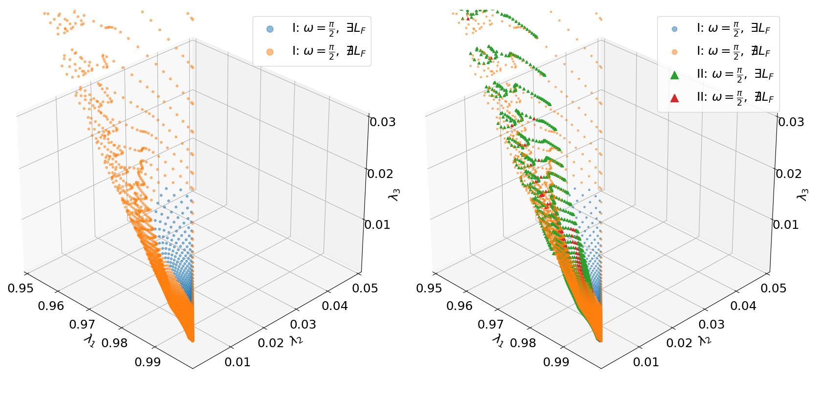
The eigenvalues of the Choi matrices are real positive numbers which sum up to $N$. The space of eigenvalues in the one-qubit problem is a three-dimensional positive manifold in the four-dimensional real space. The possibility to visualize the eigenvalues in 2D space and thus to examine the position of the points corresponding to the ’yes’ and ’no’ answers is an important advantage of this parametrization. To test this idea, we consider Problems I and II and vary values of the amplitude and frequency for a specific fixed value of the phase shift.

For every parameter set, we construct the Choi matrix and calculate its eigenvalues numerically. Further, by using the test (13), the answer to the question of the existence of Floquet-Lindbladian is obtained. The generated dataset consists of lists of eigenvalues, labeled with "0" if the answer is ’no’ and "1" if the answer is ’yes’. Fig. 1 (left) shows that the distribution of the answers is not chaotic but exhibits some structure so potentially it can be partitioned into ’yes/no’ sub-manifolds. We find this behavior typical, and the partition is present for both models, I and II, when they are considered separately. However, as it is discussed in the next section, if we plot the ’yes/no’ points for both models, without differentiating between them, we get a cloud of points which no longer exhibits signatures of partition.

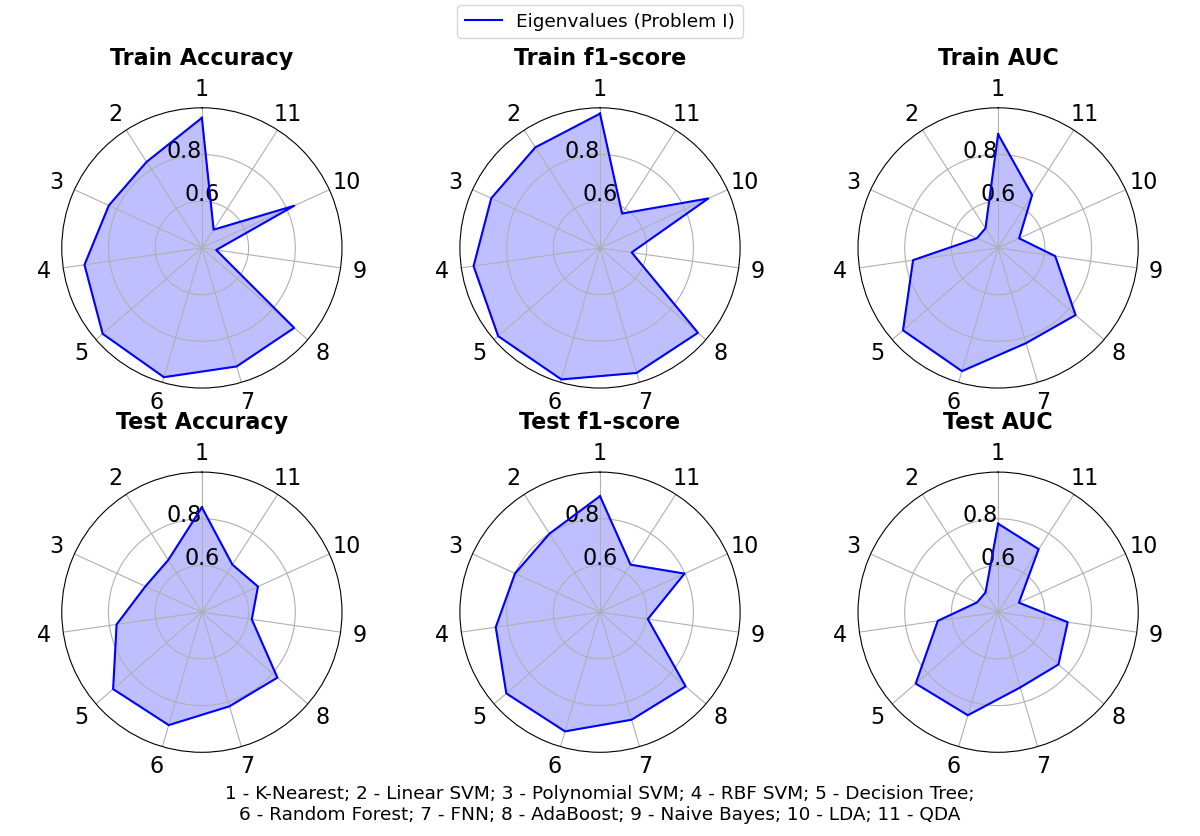
Next, we built classifiers using eleven selected ML methods. The results for Problem I are presented with Fig. 2. The main observation is that the Nearest Neighbors, Decision Tree, and Random Forest methods yield the best results (in terms of the metrics used) and significantly outperform other methods. The reason for this is that these methods compare the classified point of the parameter space with the original training sample, thereby taking into account the fact that the points are close in the sense of a particular metric. Considering by tuning the amplitude, frequency, or phase shift we do not detect substantial changes (for both problems, I and II), we conclude that the classification scheme based on the Choi eigenvalues works reasonably well.

Figure 2: Classification accuracy for datasets of Choi eigenvalues of Problem I, for training (top row) and test (bottom row) samples. The accuracy is quantified by using three different measures (see Section VA). The center of a diagram corresponds to accuracy $0.4$.

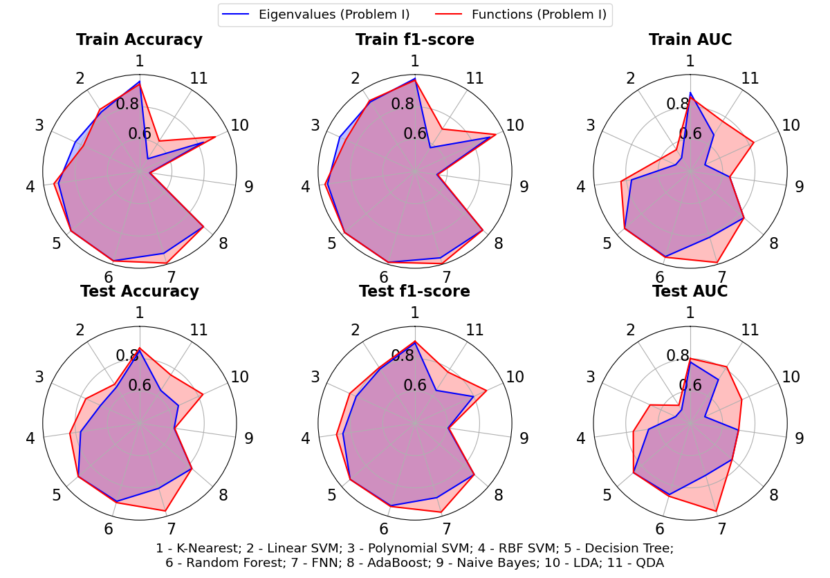
Is it possible to improve the classification? To get an insight, we expand the feature space by adding various functions of the Choi eigenvalues such as logarithms, exponents, degrees, roots, trigonometric, hyperbolic functions, and their combinations. We assume that in the extended space, methods would be able to detect linear or other, relatively simple, separability. We obtain the best separability in the space consisting of eigenvalues in powers of 1, $1/2$, and $1/4$; see Fig. 3. It is noteworthy that those methods that previously worked poorly have significantly improved their results. The fully connected neural network outperforms other methods in the sense of the classification accuracy, being able to accurately approximate the separating surface in the feature space.

Figure 3: Classification accuracy for datasets of Choi eigenvalues (blue) and of their functions, square roots and and fourth-order roots (red). Datasets were generated for Problem I. The accuracy is quantified by using three different measures (see Section VA). The center of a diagram corresponds to accuracy $0.4$.

The next important question is to what extent the developed classifiers are capable of generalization. Note that so far they were trained to solve one specific problem (Problem I or Problem II), albeit with different parameters. Now we want to check how the classifiers developed for Problem I can cope with Problem II.

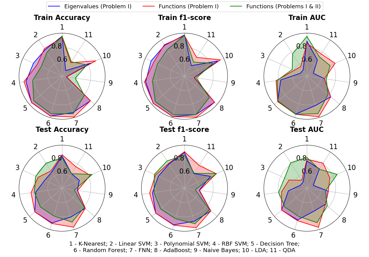
Unfortunately, the outcome is disappointing. It turns out that the models trained and validated for Problem I is not suitable for Problem II. One could say that this is expected since all methods have not seen the data obtained for Problem II during their training. However, the problems are similar and, therefore, we naturally expect the models should be able to generalize. To improve the performance, we add data obtained for Problem II to the training set. This dramatically improved the results; see Fig. 4.

However, it is still not possible to achieve results that compete with the metrics obtained during training and validating of classifiers on a single problem. The reason for this can be understood by looking at Fig. 1 (right). The presented plot shows that it is difficult to reach separability because when the samples from two problems are combined, some points appear surrounded by a cloud of points with the opposite answer. We do not present the feature space extended by various functions of the eigenvalues of the Choi matrices for this case, but obtained results make it clear that the corresponding parameterization does not lead to a better accuracy. Therefore, we should look for alternative parameterizations.

Figure 4: Classification accuracy for datasets of Choi eigenvalues (blue) and of their functions, square roots and fourth-order roots (red). Datasets were generated for Problem I. Additionally, we train and test models with mixed datasets consisting of the data for both problems, I and II (green). The accuracy is quantified by using three different measures (see Section VA). The center of a diagram corresponds to accuracy $0.4$.

V.2.2 Classification based on the elements of Choi matrices

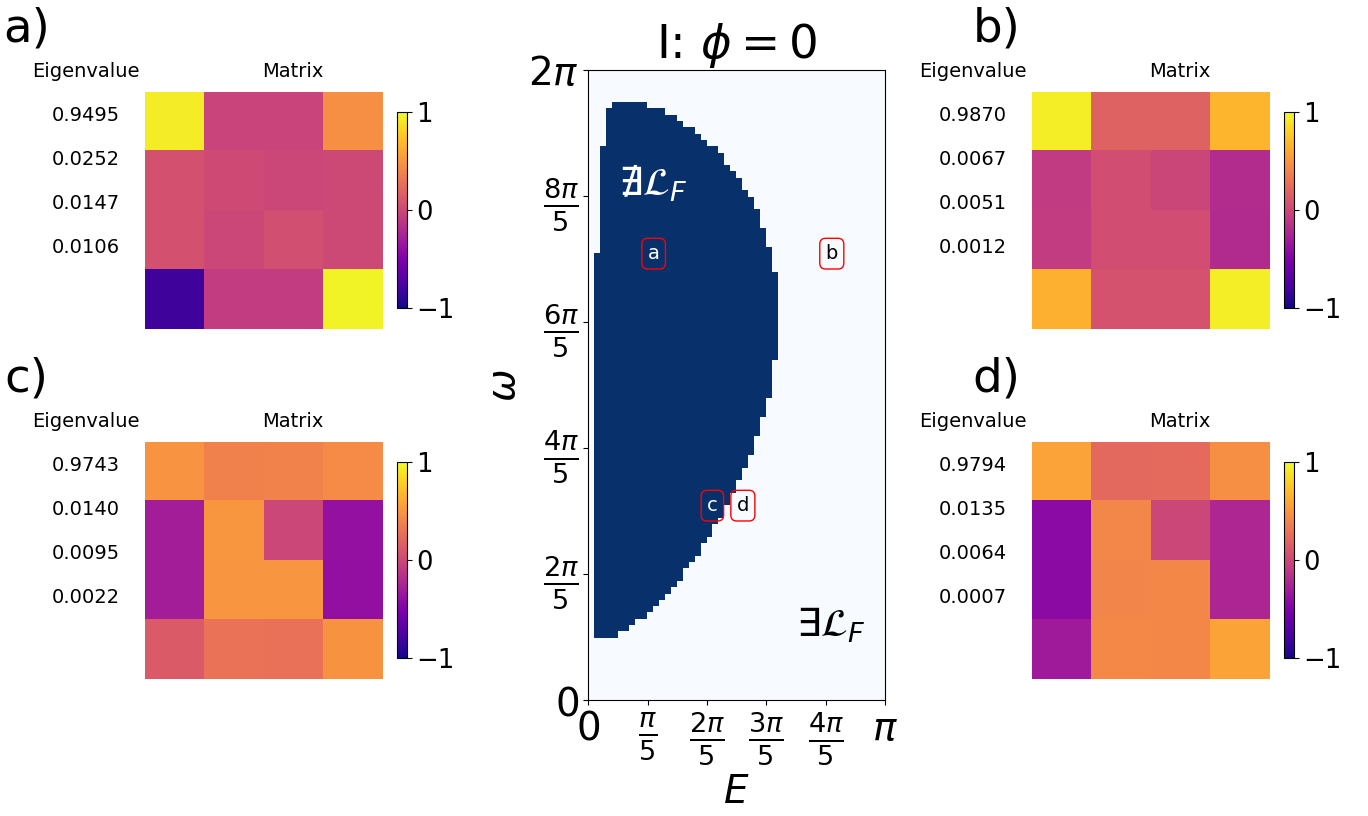
As we figured out in the previous section, the parametrization based on the eigenvalues of Choi matrices does not provide the possibility to generalize from one physical model to another model even if we add data from both models in the training dataset. Apparently, this is because such parameterization is rather reduced and we are losing too much information when condensing properties of the original Floquet map into the corresponding Choi eigenvalues. Here we try an alternative parametrization based on the elements of the Choi matrix. Namely, we use the following parameterization: the upper triangle of the matrix, including the diagonal, containing the real parts of the elements, and the lower triangle containing the imaginary parts of its elements. Such a representation is complete, since we can unambiguously restore the original data, and all the elements of the constructed matrix are real numbers. Next, we vectorize the real matrix, by writing its elements one after another column-wise. Fig. 5 presents examples of such parameterizations for four different parameters of Problem I (Figs. 5a-d).

Figure 5: Parametrization of the Choi matrix. The upper half of the matrix corresponds to the real part, the lower one – to the imaginary part of the matrix. Center: Diagram of ’yes’ (light blue) and ’no’ (dark blue) answers to the question of the existence of Floquet-Lindbladian for the Problem I. Four combinations of parameters are used (a, b, c, d). Their positions on the $(E,\omega)$ plane are indicated on the central diagram (red squares).

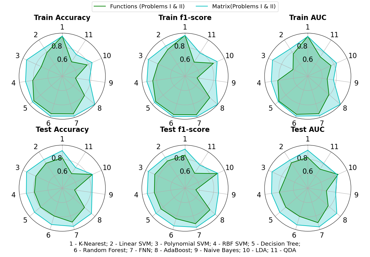
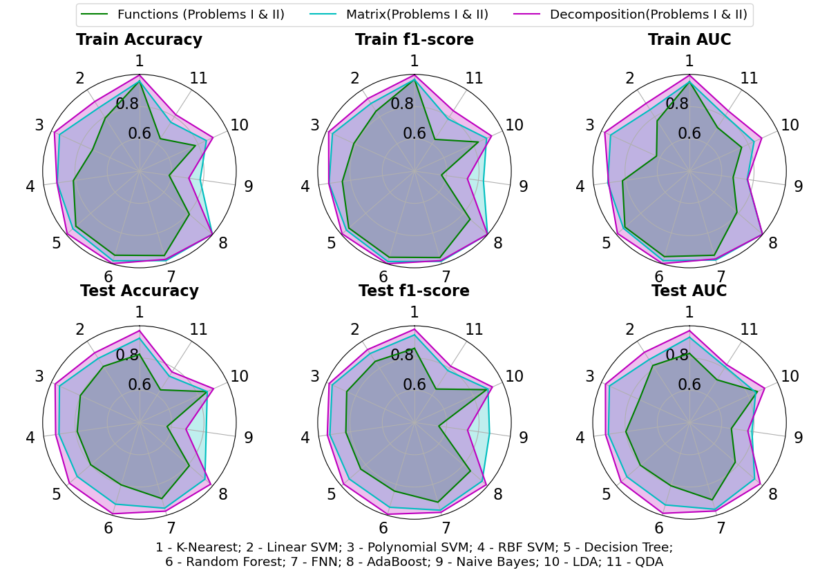
Using this parametrization, it is also possible to solve the classification problem by combining data from problems I and II both in the training and in the test samples. The best achieved results are summarized in Fig. 6. It turns out that almost all methods substantially improved their performance, both on the training sample and the test sample. AdaBoost, Neural Network, and Random Forest methods show very good results on the training set (errors less than $2.5\%$), while on the test set, the results are expected to be slightly worse in terms of accuracy.

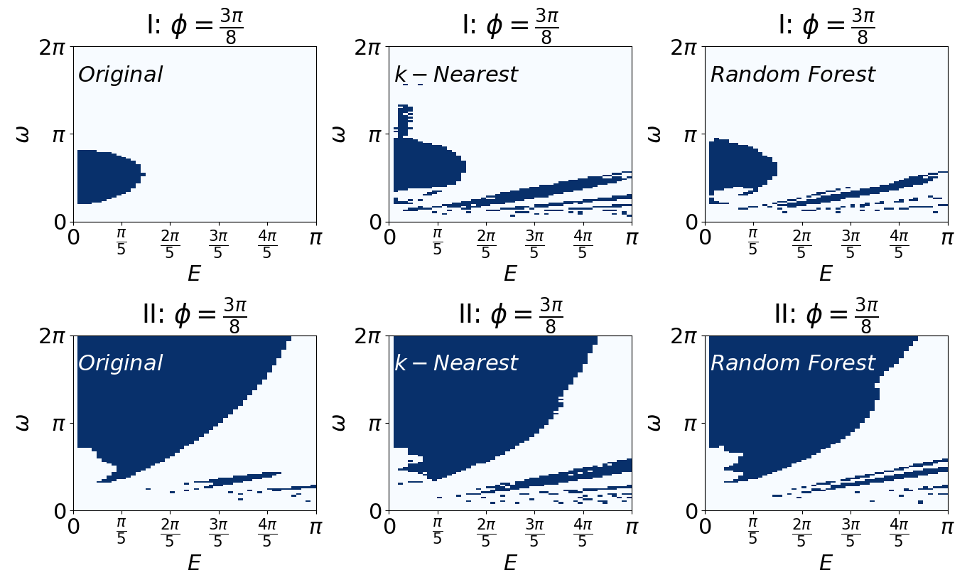
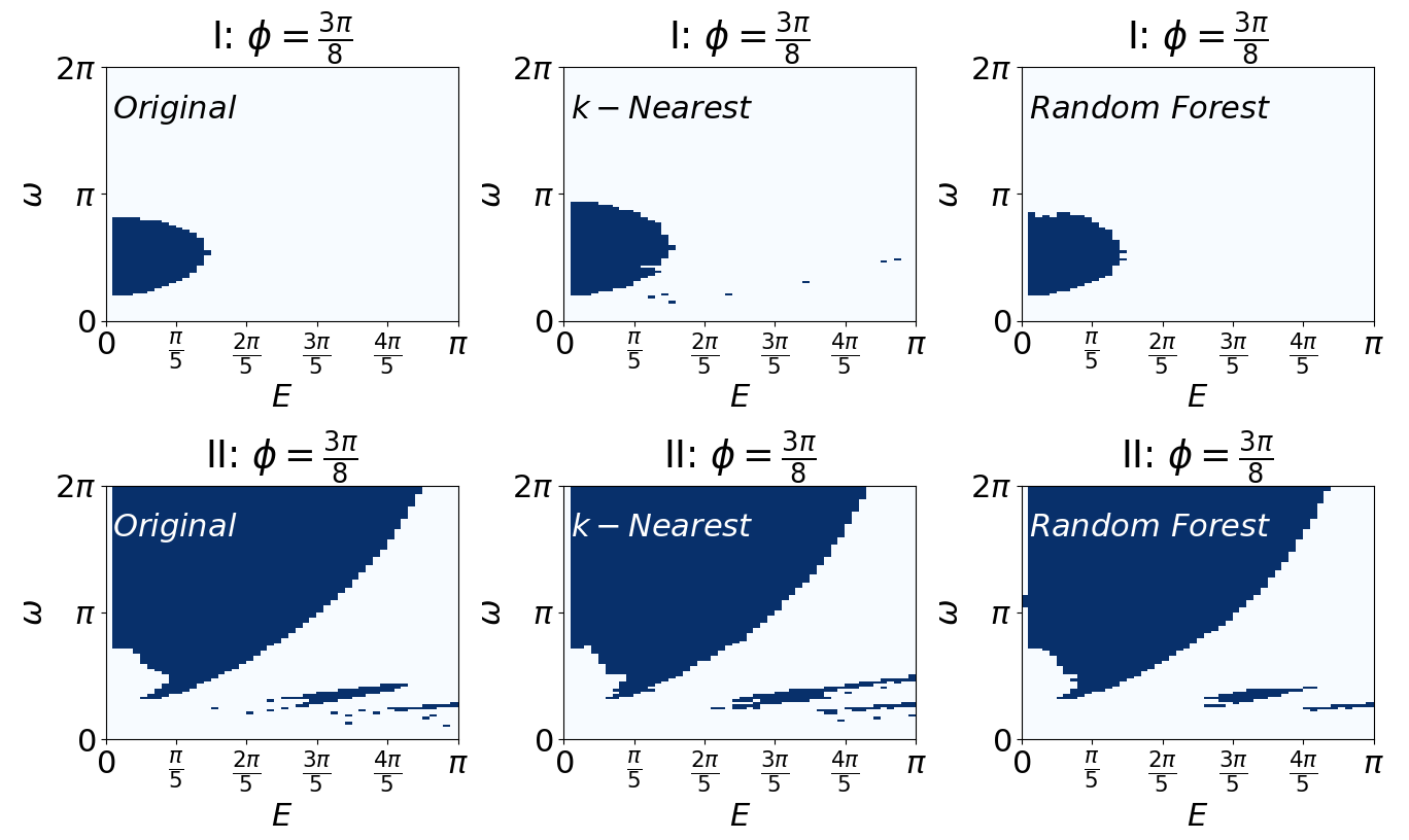
To get more insight, we inspect the two-dimensional diagram on Fig. 7 in order to understand when the classifiers are wrong. It is not correct to think that errors are localized at the vicinity of the border between the ’yes/no’ areas. The errors of this sort are expected; however, we also find error zones that are far from the border. For example, ML methods mistakenly detect extensive dark blue ‘petals’ corresponding to the answers ’no’ when solving Problem I. It is noteworthy that such ‘petals’ exist in Problem II. Obviously, having learned such ‘petals’ in one of the problems, ML methods fail to learn to recognize whether these petals are in other problems or not. We tried to overcome this problem by balancing the contribution of data from several problems in the training sample, but this did not help. Moreover, we found that ‘petals’ appear erroneously even if we only use Problem I for training and evaluation. Our conclusion is as follows: the considered parametrization is not suitable for an accurate feature selection.

It seems that even though we are using all the information encoded in the Choi matrix, the resulting approach does not lead to a better performance. The tendency is that simple models cannot generalize data from different problems and complex models are often overfitted. We conclude that we should try to identify features that are important for classification and train models on these features.

Figure 6: Classification accuracy for datasets of the Choi eigenvalues, and their functions, square roots and fourth-order roots (green) compared to the accuracy obtained by employing datasets generated by using elements of the Choi matrices (light blue). Samples from Problem I and Problem II were used for training and testing. The accuracy is quantified by using three different measures (see Section VA). The center of a diagram corresponds to accuracy $0.4$.

Figure 7: ’Yes/no’ partition of the parameter space for Problems I (top row) and II (bottom row) for different values of phase shift. Partitions are obtained by using the test, Eq. (13)[left] and ML methods, the Nearest neighbors method [center] and the Random forest method [right]. For the ML methods the parametrization based on the elements of Choi matrices is used.

V.2.3 Classification based on eigenvalues and eigenvectors of Choi matrices

Finally, We consider parameterization of a Choi matrix based on the full eigenset, which includes eigenvalues and eigenvectors. The matrix of eigenvectors is an $N^{2}\times N^{2}$ orthonormal complex matrix. It is not very convenient to use it in this form since the values of its elements vary over a wide range. Given that angles are a key feature of eigenvectors, we decided to use spherical coordinates. To use this coordinate system, we have to unfold a complex vector of size $N^{2}$ into real vectors of the size of $2N^{2}$. In this case, it is possible to make the last imaginary coordinate (the last coordinate of the real vector) equal to 0. We converted such vectors into spherical coordinates as follows:

$$\begin{gathered}r=\sqrt{x^{2}_{1}+x^{2}_{2}\dots x^{2}_{N^{2}-1}+x^{2}_{N^{2}}}\\ \varphi_{1}=\operatorname{arccot}\frac{x_{1}}{\sqrt{x^{2}_{N^{2}}+x^{2}_{{N^{2}}-1}\dots x^{2}_{3}+x^{2}_{2}}}\\ \varphi_{2}=\operatorname{arccot}\ \frac{x_{2}}{\sqrt{x^{2}_{N^{2}}+x^{2}_{{N^{2}}-1}\dots x^{2}_{4}+x^{2}_{3}}}\\ \dots{\\ }\varphi_{N^{2}-2}=\operatorname{arccot}\ \frac{x_{N^{2}-2}}{\sqrt{x^{2}_{N^{2}}+x^{2}_{N^{2}-1}}}\\ \varphi_{N^{2}-1}=\operatorname{arccot}\ \frac{x_{N^{2}-1}+\sqrt{x^{2}_{N^{2}}+x^{2}_{N^{2}-1}}}{x^{2}_{N^{2}}}\end{gathered}$$

This approach has several advantages:

1. There is no loss of information, that is, the original data (Floquet map) can be reconstructed.

2. The length of the vector is equal to 1 (and therefore is irrelevant).

3. We can exclude the coordinate of the angle $\varphi_{N^{2}-1}\in[0,2\pi]$ from the data, since it is equal to zero during computation for the zero component. Thus, the angles close to 0 and $2\pi$ are not close to each other in the generated data.

4. All other angles $\varphi_{i}\in[0,\pi]$, and represent an ordinary hypercube.

All angles were also normalized to the range $[0,1]$ to get rid of unnecessary dependence on $\pi$.

Figure 8: ’Yes/no’ partition of the parameter space for Problems I (top row) and II (bottom row) for different values of phase shift. Partitions are obtained by using the test, Eq. (13) [left] and ML methods, the Nearest neighbors method [center] and the Random forest method [right]. For the ML methods the parametrization based on the eigenvalues and eigenvectors of Choi matrices is used.

After constructing the classifiers, we implement the same training procedure as in the previous section, by using datasets obtained with both models, I and II. We find that the results are substantially better; see Fig. 8. However, there are still regions of wrong answers far from the ’yes/nor’ border. As before, in some cases in Problem I, the petals of answers ’no’ were mistakenly found in those areas of parameters in which these petal-like regions are present in Problem II. We analyze the datasets to understand the origin of this behavior. We find that the adjacent points on the diagram are distinguished by a smooth change in the angles corresponding to real-valued coordinates, and by sharp changes in the angles corresponding to complex-valued coordinates. As a result, ML methods at some point begin to ’react’ only to dramatic changes of the values, which leads to the decay of the accuracy of classification. To overcome this effect, we remove angles corresponding to the complex-valued coordinates from the datasets. After purging the data, we evidently are no longer able to reconstruct the original matrix, however we expect that this purge could improve the accuracy of classification. Fig. 9 reports the obtained results.

First of all, the accuracy of every classifier has improved. Most of the methods now give correct answers, both on the training and test samples, in more than $90\%$ of the cases. Next, we concentrate on further improving the accuracy of the methods that give the best results by performing some balancing in the feature space. We notice that changes in the eigenvalues contribute less to the classification results because the sum of all eigenvalues is equal to 2, but each of the angles corresponding to the eigenvectors varies from 0 to 1. To achieve more homogeneity, we use the following transformation:

$$\lambda^{\prime}=0.5(\lambda-0.5)\begin{pmatrix}1&1&1&1\\ 1&-1&-1&1\\ -1&1&-1&1\\ -1&-1&1&1\end{pmatrix}$$ (19)

After performing the transformation, we get three non-zero values, which are distributed from 0 to 1. Fig. 10 shows the distributions of eigenvalues before and after the transformation.

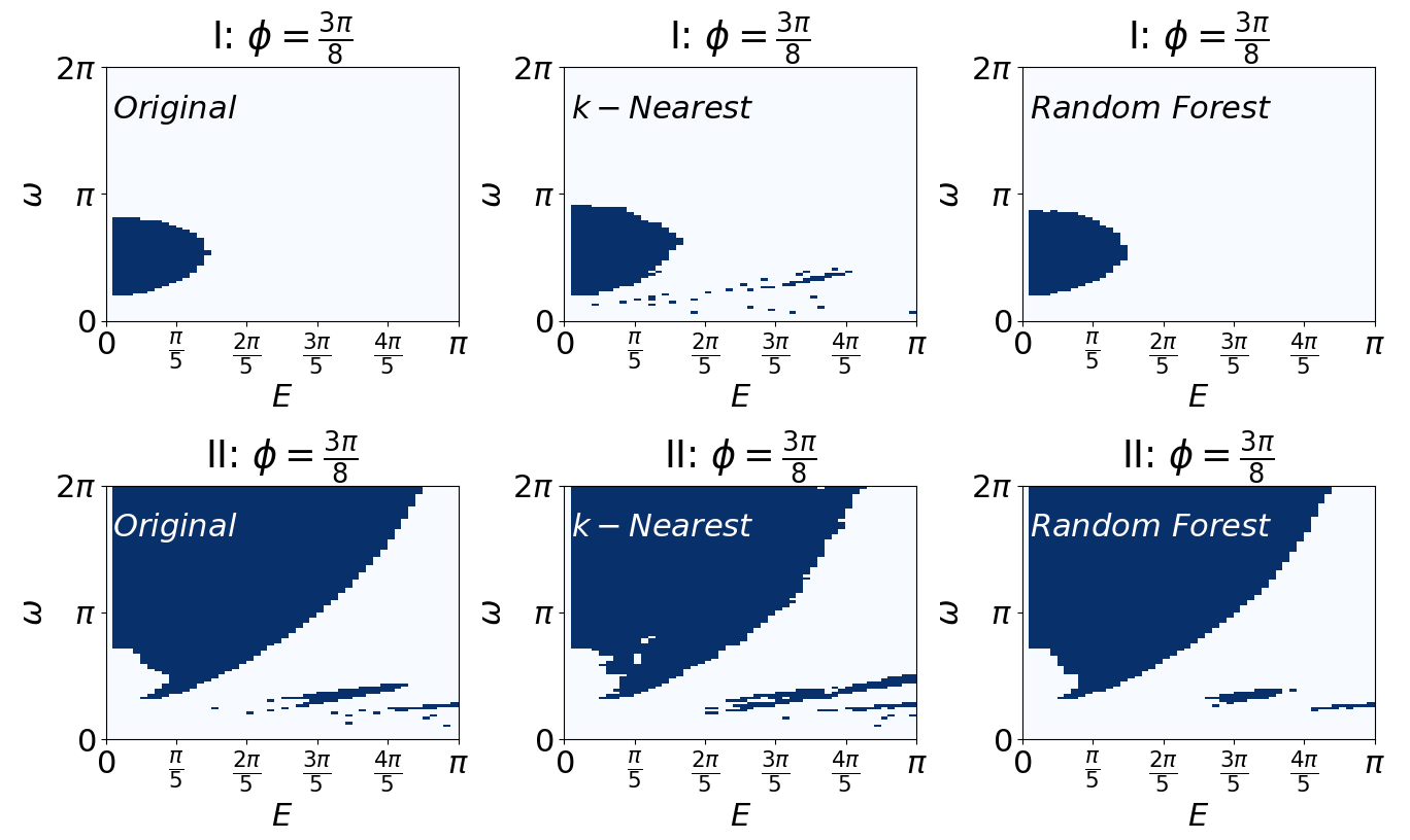
The obtained results demonstrate that after the transformation, the first eigenvalue does no longer dominates over the rest of the eigenvalues. Further on, we scale the values of the angles from the interval $[0,1]$ to the interval $[0,0.25]$ in order to increase the importance of the contribution of eigenvalues to the classification results. All this improves the accuracy even of the methods that previously did not work well. The final results are summarized in Table 1 and Fig. 11. The diagram shown in Fig. 11 highlights that the classification errors have local characters and there are no wrong-answer regions appear.

Figure 9: Classification accuracy for three datasets: a) generated by using the Choi eigenvalues and their functions, square roots and fourth-order roots (green); b) generated by using elements of the Choi matrices (light blue); c) generated by using the Choi eigenvalues and eigenvectors after appropriate normalization (magenta). Samples from Problem I and Problem II were used for training and testing. The accuracy is quantified by using three different measures (see Section VA). The center of a diagram corresponds to accuracy $0.4$.

Figure 10: The distribution of the eigenvalues of Choi matrices before (top row) and after (bottom row) the transformation, Eq. (17).

Figure 11: ’Yes/no’ partition of the parameter space for Problems I (top row) and II (bottom row) for different values of phase shift. Partitions are obtained by using the test, Eq. (13) [left] and ML methods, the Nearest neighbors method [center] and the Random forest method [right]. For the ML methods the parametrization based on the eigenvalues, normalized with the transformation (17), and eigenvectors of Choi matrices, is used.

Method	Train %	Test %	Train f1	Test f1	Train AUC	Test AUC
Random Forest (Decomposition)	0.998	0.990	0.999	0.993	0.998	0.987
AdaBoost (Decomposition)	0.999	0.984	0.999	0.989	0.999	0.980
AdaBoost (with Normalization)	0.999	0.989	0.999	0.992	0.999	0.987

Table 1: The best achieved classification accuracy metrics for a dataset of the eigenvalues and eigenvectors of Choi matrices. Samples from Problem I and Problem II were used for training and testing.

VI Conclusion

In this work, we estimated the potential of Machine Learning (ML) methods as tools to analyze the Floquet-Lindbladian (FL) problem. We put the emphasis on finding appropriate feature space for which it is possible to construct and train high-accuracy classifiers. As a start, we considered the feature space constructed by using the eigenvalues of the Choi matrices and found that even though good accuracy can be achieved with one model, it is not possible to generalize the obtained classifiers to another problem. Next, we use the whole sets of elements of the Choi matrices. However, this approach did not yield encouraging results either. Finally, by taking into account all the elements of the eigenset, that are eigenvalues and eigenvectors of the Choi matrix, we managed to develop a procedure to purge and normalize data, which allowed us to reach more than $90\%$ of the classification accuracy when solving the FL problem for both models.

Even though the results we obtained are encouraging and motivating, we should not overestimate the perspectives since we are having a situation rather typical to the ML and AI fields when the results are usually very promising for small-scale test problems. First of all, we cannot prove that the developed schemes would work if the problem set-up is substantially modified. Next, it is not known whether it will be possible to generalize the results to higher values of $N$ (which is our main motivation).

However, our results provide insight into the mathematical nature of the original problem Davies et al. (2021). For example, the fact that, by taking into account not only eigenvalues of the Choi matrix but also eigenvectors, we have obtained substantially better accuracy, tells that some physically relevant information about Markovianity of the map is encoded in the eigenvectors of its Choi matrix. Since the test, Eq. (13), contains matrices derived from the eigenelements of the Floquet map, we could assume that eigenvectors of the Choi matrix also bear information about the degree of Markoviaity of the original Floquet map. Our results validate this assumption and thus constitute, as we believe, a step in the understanding of the Floquet-Lindbladian problem.

Data Availability

Data sharing is not applicable to this article as no new data were created or analyzed in this study.

References

- Elfving (1937) G. Elfving, “Zur Theorie der Markoffschen Ketten,” Acta Societatis Scientiarum Fennicae 2, 4–11 (1937).
- Wolf et al. (2008) M. Wolf, J. Eisert, T. Cubitt, and J. Cirac, “Assessing non-Markovian quantum dynamics,” Physical review letters 101, 150402 (2008).
- Cubitt, Eisert, and Wolf (2012) T. S. Cubitt, J. Eisert, and M. M. Wolf, “The complexity of relating quantum channels to master equations,” Communications in Mathematical Physics 310, 383–418 (2012).
- Garey and Johnson (1979) M. R. Garey and D. S. Johnson, Computers and intractability: A guide to the theory of NP-Completeness (Series of Books in the Mathematical Sciences), first edition ed. (W. H. Freeman, 1979).
- Volokitin et al. (2022) V. Volokitin, E. Kozinov, A. Liniov, I. Yusipov, S. Veselov, N. Zolotykh, M. Ivanchenko, I. Meyerov, and S. Denisov, “Is there a Lindbladian? Implementation of the test,” (in preparation) (2022).
- Holthaus (2015) M. Holthaus, “Floquet engineering with quasienergy bands of periodically driven optical lattices,” Journal of Physics B: Atomic, Molecular and Optical Physics 49, 013001 (2015).
- Bukov, D’Alessio, and Polkovnikov (2015) M. Bukov, L. D’Alessio, and A. Polkovnikov, “Universal high-frequency behavior of periodically driven systems: from dynamical stabilization to Floquet engineering,” Advances in Physics 64, 139–226 (2015).
- Schnell, Eckardt, and Denisov (2020) A. Schnell, A. Eckardt, and S. Denisov, “Is there a Floquet Lindbladian?” Physical Review B 101, 100301 (2020).
- Yusipov et al. (2021) I. I. Yusipov, V. D. Volokitin, A. V. Liniov, M. V. Ivanchenko, I. B. Meyerov, and S. V. Denisov, “Machine Learning versus Semidefinite Programming approach to a particular problem of the theory of open quantum systems,” Lobachevskii Journal of Mathematics 42, 1622–1629 (2021).
- Zhang (2016) Z. Zhang, “Introduction to Machine Learning: K-Nearest Neighbors,” Annals of Translational Medicine 4, 218–218 (2016).
- Kramer (2013) O. Kramer, “K-Nearest Neighbors,” in Dimensionality reduction with unsupervised Nearest Neighbors (Springer Berlin Heidelberg, Berlin, Heidelberg, 2013) pp. 13–23.
- Suykens and Vandewalle (1999) J. A. K. Suykens and J. Vandewalle, “Least Squares Support Vector Machine Classifiers,” Neural Processing Letters 9, 293–300 (1999).
- Amari and Wu (2001) S. Amari and S. Wu, “Improving support Vector Machine Classifiers by modifying kernel functions,” Neural Networks 12, 783–789 (2001).
- Dagher (2008) I. Dagher, “Quadratic kernel-Free non-linear Support Vector Machine,” Journal of Global Optimization 41, 15–30 (2008).
- Breuer (2004) H.-P. Breuer, “Genuine quantum trajectories for non-Markovian processes,” Physical Review A 70, 012106 (2004).
- Breuer, Laine, and Piilo (2009) H.-P. Breuer, E.-M. Laine, and J. Piilo, “Measure for the degree of non-Markovian behavior of quantum processes in open systems,” Physical Review Letters 103, 210401 (2009).
- Gorini, Kossakowski, and Sudarshan (1976) V. Gorini, A. Kossakowski, and E. C. G. Sudarshan, “Completely positive dynamical semigroups of N-Level systems,” Journal of Mathematical Physics 17, 821 (1976).
- Lindblad (1976) G. Lindblad, “On the generators of quantum dynamical semigroups,” Communications of Mathematical Physics 48, 119–130 (1976).
- Khachiyan and Porkolab (1997) L. Khachiyan and L. Porkolab, “Computing integral points in Convex semi-algebraic sets,” in Proceedings 38th Annual Symposium on Foundations of Computer Science (1997) pp. 162–171.
- Flum and Grohe (2006) J. Flum and M. Grohe, Parameterized Complexity Theory (Texts in Theoretical Computer Science. An EATCS Series) (Springer-Verlag, Berlin, Heidelberg, 2006).
- Carleo et al. (2019) G. Carleo, I. Cirac, K. Cranmer, L. Daudet, M. Schuld, N. Tishby, L. Vogt-Maranto, and L. Zdeborová, “Machine Learning and the Physical Sciences,” Reviews of Modern Physics 91, 045002 (2019).
- Choi (1975) M.-D. Choi, “Completely positive linear maps on complex matrices,” Linear Algebra and its Applications 10, 285–290 (1975).
- Życzkowski and Bengtsson (2004) K. Życzkowski and I. Bengtsson, “On duality between quantum states and quantum maps,” Open Systems & Information Dynamics 11, 3–42 (2004).
- Boyd et al. (1994) S. Boyd, L. El Ghaoui, E. Feron, and V. Balakrishnan, Linear matrix inequalities in system and control theory (Society for Industrial and Applied Mathematics, 1994).
- Ramana and Goldman (1995) M. Ramana and A. J. Goldman, “Some geometric results in semidefinite programming,” Journal of Global Optimization 7, 33–50 (1995).
- Pedregosa et al. (2011) F. Pedregosa, G. Varoquaux, A. Gramfort, V. Michel, B. Thirion, O. Grisel, M. Blondel, P. Prettenhofer, R. Weiss, V. Dubourg, J. Vanderplas, A. Passos, D. Cournapeau, M. Brucher, M. Perrot, and E. Duchesnay, “Scikit-learn: Machine Learning in Python,” Journal of Machine Learning Research 12, 2825–2830 (2011).
- Safavian and Landgrebe (1991) S. Safavian and D. Landgrebe, “A Survey of decision Tree Classifier methodology,” IEEE Transactions on Systems, Man, and Cybernetics 21, 660–674 (1991).
- Breiman et al. (1984) L. Breiman, J. H. Friedman, R. A. Olshen, and C. J. Stone, Classification and Regression Trees (Wadsworth International Group, Belmont, CA, 1984).
- Cutler, Cutler, and Stevens (2012) A. Cutler, D. R. Cutler, and J. R. Stevens, “Random Forests,” in Ensemble Machine Learning: Methods and Applications, edited by C. Zhang and Y. Ma (Springer US, Boston, MA, 2012) pp. 157–175.
- Breiman (2001) L. Breiman, “Random Forests,” Machine Learning 45, 5–32 (2001).
- Sanger (1989) T. D. Sanger, “Optimal Unsupervised Learning in a single-layer linear Feedforward Neural Network,” Neural networks 2, 459–473 (1989).
- Glorot and Bengio (2010) X. Glorot and Y. Bengio, “Understanding the difficulty of training Deep Feedforward Neural Networks,” in Proceedings of the Thirteenth International Conference on Artificial Intelligence and Statistics, JMLR Proceedings, Vol. 9, edited by Y. W. Teh and D. M. Titterington (JMLR.org, 2010) pp. 249–256.
- Freund and Schapire (1997) Y. Freund and R. E. Schapire, “A decision-theoretic generalization of on-line learning and an application to boosting,” Journal of Computer and System Sciences 55, 119–139 (1997).
- Fukunaga (2013) K. Fukunaga, Introduction to Statistical Pattern Recognition (Elsevier, 2013).
- Domingos and Pazzani (1997) P. Domingos and M. Pazzani, “On the optimality of the simple Bayesian classifier under zero-one Loss,” Machine Learning 29, 103–130 (1997).
- Chicco and Jurman (2020) D. Chicco and G. Jurman, “The Aavantages of the Matthews Correlation Coefficient (MCC) over F1 Score and accuracy in Binary Classification Evaluation,” BMC Genomics 21 (2020), 10.1186/s12864-019-6413-7.
- Fawcett (2006) T. Fawcett, “An introduction to ROC analysis,” Pattern Recognition Letters 27, 861–874 (2006).
- Davies et al. (2021) A. Davies et al., “Advancing mathematics by guiding human intuition with AI,” Nature 600, 70–74 (2021).