Batched Second-Order Adjoint Sensitivity for Reduced Space Methods

Abstract

This paper presents an efficient method for extracting the second-order sensitivities from a system of implicit nonlinear equations on upcoming graphical processing units (GPU) dominated computer systems. We design a custom automatic differentiation (AutoDiff) backend that targets highly parallel architectures by extracting the second-order information in batch. When the nonlinear equations are associated to a reduced space optimization problem, we leverage the parallel reverse-mode accumulation in a batched adjoint-adjoint algorithm to compute efficiently the reduced Hessian of the problem. We apply the method to extract the reduced Hessian associated to the balance equations of a power network, and show on the largest instances that a parallel GPU implementation is 30 times faster than a sequential CPU reference based on UMFPACK

1 Introduction

System of nonlinear equations are ubiquitous in numerical computing. Solving such nonlinear systems typically depends on efficient iterative algorithms, as for example Newton-Raphson. In this article, we are interested in the resolution of a parametric system of nonlinear equations, where the solution depends on a vector of parameters $\bm{p}\in\mathbb{R}^{n_{p}}$. These parametric systems are, in their abstract form, written as

(1.1) $$\text{Find }\bm{x}\text{ such that }g(\bm{x},\bm{p})=0\;,$$

where the (smooth) nonlinear function $g:\mathbb{R}^{n_{x}}\times\mathbb{R}^{n_{p}}\to\mathbb{R}^{n_{x}}$ depends jointly on an unknown variable $\bm{x}\in\mathbb{R}^{n_{x}}$ and the parameters $\bm{p}\in\mathbb{R}^{n_{p}}$.

The solution $x(\bm{p})$ of (1.1) depends implicitly on the parameters $\bm{p}$: of particular interest are the sensitivities of the solution $x(\bm{p})$ with relation to the parameters $\bm{p}$. Indeed, these sensitivities can be embedded inside an optimization algorithm (if $\bm{p}$ is a design variable) or in an uncertainty quantification scheme (if $\bm{p}$ encodes an uncertainty). It is well known that propagating the sensitivities in an iterative algorithm is nontrivial [12]. Fortunately, there is no need to do so, as we can exploit the mathematical structure of (1.1) and compute directly the sensitivities of the solution $x(\bm{p})$ using the Implicit Function Theorem.

By repeating this process one more step, we are able to extract second-order sensitivities at the solution $x(\bm{p})$. However, this operation is computationally more demanding and involves the manipulation of third-order tensors $\nabla^{2}_{\bm{x}\bm{x}}g,\nabla^{2}_{\bm{x}\bm{p}}g,\nabla^{2}_{\bm{p}\bm{p}}g$. The challenge is to avoid forming explicitly such tensors by using reverse mode accumulation of second-order information, either explicitly by using the specific structure of the problem --- encoded by the function $g$ --- or by using automatic differentiation.

Figure 1: Reduced space algorithm. This article focuses on the last block, in red. If $F$ is an objective function, the reduced gradient $\nabla_{\bm{p}}F$ and the reduced Hessian $\nabla^{2}_{\bm{p}\bm{p}}F$ can be used in any nonlinear optimization algorithm.

As illustrated in Figure 1, this paper covers the efficient computation of the second-order sensitivities of a nonlinear system (1.1). The sparsity structure of the problem is passed to a custom Automatic Differentiation (AutoDiff) backend that automatically generates all the intermediate sensitivities from the implementation of $g(\bm{x},\bm{p})$. To get a tractable algorithm, we use an adjoint model implementation of the generated first-order sensitivities to avoid explicitly forming third-order derivative tensors. As an application, we compute the reduced Hessian of the nonlinear equations corresponding to the power flow balance equations of a power grid [29]. The problem has an unstructured graph structure, leading to some challenge in the automatic differentiation library, that we discuss extensively. We show that the reduced Hessian associated to the power flow equations can be computed efficiently in parallel, by using batches of Hessian-vector products. The underlying motivation is to embed the reduction algorithm in a real-time tracking procedure [28], where the reduced Hessian updates have to be fast to track a suboptimal solution.

In summary, we aim at devising a portable, efficient, and easily maintainable reduced Hessian algorithm. To this end, we leverage the expressiveness offered by the Julia programming language. Due to the algorithm’s design, the automatic differentiation backend and the reduction algorithm are transparently implemented on the GPU without any changes to the algorithm’s core implementation, thus realizing a composable software design.

1.1 Contributions

Our contribution is a tractable SIMD algorithm and implementation to evaluate the reduced Hessian from a parametric system of nonlinear equations (1.1). This consists of three closely intertwined components. First, we implement the nonlinear function $g(\bm{x},\bm{p})$ using the programming language Julia [6] and the portability layer KernelAbstractions.jl to generate abstract kernels working on various GPU architectures (CUDA, ROCm). Second, we develop a custom AutoDiff backend on top of the portability layer to extract automatically the first-order sensitivities $\nabla_{\bm{x}}g,\nabla_{\bm{p}}g$ and the second-order sensitivities $\nabla_{\bm{x}\bm{x}}^{2}g,\nabla_{\bm{x}\bm{p}}^{2}g,\nabla_{\bm{p}\bm{p}}^{2}g$. Third, we combine these in an efficient parallel accumulation of the reduced Hessian associated to a given reduced space problem. The accumulation involves both Hessian tensor contractions and two sparse linear solves with multiple right-hand sides. Glued together, the three components give a generic code able to extract the second-order derivatives from a power grid problem, running in parallel on GPU architectures. Numerical experiments with Volta GPUs (V100) showcase the scalability of the approach, reaching a 30x faster computation on the largest instances when compared to a reference CPU implementation using UMFPACK. Current researches suggest that a parallel OpenMP power flow implementation using multi-threading (on the CPU alone) potentially achieves a speed-up of 3 [2] or up to 7 and 70 speed-up for Newton-Raphson and batched Newton-Raphson [30], respectively. However, multi-threaded implementations are not the scope of this paper as we focus on architectures where GPUs are the dominant FLOP contributors for our specific application of second-order space reduction.

2 Prior Art

In this article we extract the second-order sensitivities from the system of nonlinear equations using automatic differentiation (AutoDiff). AutoDiff on Single Instruction, Multiple Data (SIMD) architectures alike the CUDA cores on GPUs is an ongoing research effort. Forward-mode AutoDiff effectively adds tangent components to the variables and preserves the computational flow. In addition, a vector mode can be applied to propagate multiple tangents or directional derivatives at once. The technique of automatically generating derivatives of function implementations has been investigated since the 1950s [22, 4].

Reverse- or adjoint-mode AutoDiff reverses the computational flow and thus incurs a lot of access restrictions on the final code. Every read of a variable becomes a write, and vice versa. This leads to application-specific solutions that exploit the structure of an underlying problem to generate efficient adjoint code [8, 13, 15]. Most prominently, the reverse mode is currently implemented as backpropagation in machine learning. Indeed, the backpropagation has a long history (e.g., [9]) with the reverse mode in AutoDiff being formalized for the first time in [18]. Because of the limited size and single access pattern of neural networks, current implementations [24, 1, 16] reach a high throughput on GPUs. For the wide field of numerical simulations, however, efficient adjoints of GPU implementations remain challenging [20]. In this work we combine the advantages of GPU implementations of the gradient with the evaluation of Hessian-vector products first introduced in [25].

Reduced-space methods have been applied widely in uncertainty quantification and partial differential equation (PDE)-constrained optimization [7], and their applications in the optimization of power grids is known since the 1960s [11]. However, extracting the second-order sensitivities in the reduced space has been considered tedious to implement and hard to motivate on classical CPU architectures (see [17] for a recent discussion about the computation of the reduced Hessian on the CPU). To the best of our knowledge, this paper is the first to present a SIMD focused algorithm leveraging the GPU to efficiently compute the reduced Hessian of the power flow equations.

3 Reduced space problem

In Section 3.1 we briefly introduce the power flow nonlinear equations to motivate our application. We present in Section 3.2 the reduced space problem associated with the power flow problem, and recall in Section 3.3 the first-order adjoint method, used to evaluate efficiently the gradient in the reduced space, and later applied to compute the adjoint of the sensitivities.

3.1 Presentation of the power flow problem.

We present a brief overview of the steady-state solution of the power flow problem. The power grid can be described as a graph $\mathcal{G}=\{V,E\}$ with $n_{v}$ vertices and $n_{e}$ edges. The steady state of the network is described by the following nonlinear equations, holding at all nodes $i\in V$,

(3.2) $$\left\{\begin{aligned} P_{i}^{inj}&=v_{i}\sum_{j\in A(i)}v_{j}(g_{ij}\cos{(\theta_{i}-\theta_{j})}+b_{ij}\sin{(\theta_{i}-\theta_{j}}))\,,\\ Q_{i}^{inj}&=v_{i}\sum_{j\in A(i)}v_{j}(g_{ij}\sin{(\theta_{i}-\theta_{j})}-b_{ij}\cos{(\theta_{i}-\theta_{j}}))\,,\end{aligned}\right.$$

where at node $i$, $(P_{i}^{inj}$ and $Q_{i}^{inj})$ are respectively the active and reactive power injections; $v_{i}$ is the voltage magnitude; $\theta_{i}$ the voltage angle; and $A(i)\subset V$ is the set of adjacent nodes: for all $j\in A(i)$, there exists a line $(i,j)$ connecting node $i$ and node $j$. The values $g_{ij}$ and $b_{ij}$ are associated with the physical characteristics of the line $(i,j)$. Generally, we distinguish the (PV) nodes --- associated to the generators --- from the (PQ) nodes comprising only loads. We note that the structure of the nonlinear equations (3.2) depends on the structure of the underlying graph through the adjacencies $A(\cdot)$.

We rewrite the nonlinear equations (3.2) in the standard form (1.1). At all nodes the power injection $P^{inj}_{i}$ should match the net production $P_{i}^{g}$ minus the load $P_{i}^{d}$:

(3.3) $$g(\bm{x},\bm{p})=\begin{bmatrix}\bm{P}_{pv}^{inj}-\bm{P}^{g}+\bm{P}_{pv}^{d}\\ \bm{P}_{pq}^{inj}+\bm{P}_{pq}^{d}\\ \bm{Q}_{pq}^{inj}+\bm{Q}_{pd}^{d}\end{bmatrix}=0~{}\text{with}~{}\bm{x}=\begin{bmatrix}\bm{\theta}^{pv}\\ \bm{\theta}^{pq}\\ \bm{v}^{pq}\end{bmatrix}\,.$$

In (3.3), we have selected only a subset of the power flow equations (3.2) to ensure that the nonlinear system $g(\bm{x},\bm{p})=0$ is invertible with respect to the state $\bm{x}$. The unknown variable $\bm{x}$ corresponds to the voltage angles at the PV and PQ nodes and the voltage magnitudes at the PQ nodes. However, in contrast to the variable $\bm{x}$, we have some flexibility in choosing the parameters $\bm{p}$.

In optimal power flow (OPF) applications, we are looking at minimizing a given operating cost $f:\mathbb{R}^{n_{x}}\times\mathbb{R}^{n_{p}}\to\mathbb{R}$ (associated to the active power generations $\bm{P}^{g}$) while satisfying the power flow equations (3.3). In that particular case, $\bm{p}$ is a design variable associated to the active power generations and the voltage magnitude at PV nodes:  $\bm{p}=(\bm{P}^{g},\bm{v}_{pv})$. We define the OPF problem as

(3.4) $$\min_{\bm{x},\bm{p}}\;f(\bm{x},\bm{p})~{}\text{ subject to }g(\bm{x},\bm{p})=0\;.$$

3.2 Projection in the reduced space.

We note that in Equation (3.3), the functional $g$ is continuous and that the dimension of the output space is equal to the dimension of the input variable $\bm{x}$. Thanks to the particular network structure of the problem (encoded by the adjacencies $A(\cdot)$ in (3.2)), the Jacobian $\nabla_{\bm{x}}g$ is sparse.

Generally, the nonlinear system (3.3) is solved iteratively with a Newton-Raphson algorithm. If at a fixed parameter $\bm{p}$ the Jacobian $\nabla_{\bm{x}}g$ is invertible, we compute the solution $x(\bm{p})$ iteratively, starting from an initial guess $\bm{x}_{0}$: $\bm{x}_{k+1}=\bm{x}_{k}-(\nabla_{\bm{x}}g_{k})^{-1}g(\bm{x}_{k},\bm{p})$ for $k=1,\dots,K$. We know that if $\bm{x}_{0}$ is close enough to the solution, then the convergence of the algorithm is quadratic.

With the projection completed, the optimization problem (3.4) rewrites in the reduced space as

(3.5) $$\min_{\bm{p}}\;F(\bm{p}):=f\big{(}x(\bm{p}),\bm{p}\big{)}\;,$$

reducing the number of optimization variables from $n_{x}+n_{p}$ to $n_{p}$, while at the same time eliminating all equality constraints in the formulation.

3.3 First-Order Adjoint Method.

With the reduced space problem (3.5) defined, we compute the reduced gradient $\nabla_{\bm{p}}F$ required for the reduced space optimization routine. By definition, as $x(\bm{p})$ satisfies $g(x(\bm{p}),\bm{p})=0$, the chain rule yields $\nabla_{\bm{p}}F=\nabla_{\bm{p}}f+\nabla_{\bm{x}}f\cdot\nabla_{\bm{p}}x$ with $\nabla_{\bm{p}}x=-\big{(}\nabla_{\bm{x}}g)^{-1}\nabla_{\bm{p}}g$. However, evaluating the full sensitivity matrix $\nabla_{\bm{p}}x$ involves the resolution of $n_{x}$ linear system. On the contrary, the adjoint method requires solving a single linear system. For every dual $\bm{\lambda}\in\mathbb{R}^{n_{x}}$, we introduce a Lagrangian function defined as

(3.6) $$\ell(\bm{x},\bm{p},\bm{\lambda}):=f(\bm{x},\bm{p})+\bm{\lambda}^{\top}g(\bm{x},\bm{p})\;.$$

If $\bm{x}$ satisfies $g(\bm{x},\bm{p})=0$, then the Lagrangian $\ell(\bm{x},\bm{p},\bm{\lambda})$ does not depend on $\bm{\lambda}$ and we get $\ell(\bm{x},\bm{p},\bm{\lambda})=F(\bm{p})$. By using the chain rule, the total derivative of $\ell$ with relation to the parameter $\bm{p}$ satisfies

$$d_{p}\ell =\big{(}\nabla_{\bm{x}}f\cdot\nabla_{\bm{p}}x+\nabla_{\bm{p}}f\big{)}+\bm{\lambda}^{\top}\big{(}\nabla_{\bm{x}}g\cdot\nabla_{\bm{u}}x+\nabla_{\bm{p}}g\big{)}$$

$$=\big{(}\nabla_{\bm{p}}f+\bm{\lambda}^{\top}\nabla_{\bm{p}}g\big{)}+\big{(}\nabla_{\bm{x}}f+\bm{\lambda}^{\top}\nabla_{\bm{x}}g\big{)}\nabla_{\bm{p}}x\;.$$

We observe that by setting the first-order adjoint to $\bm{\lambda}=-(\nabla_{\bm{x}}g)^{-\top}\nabla_{\bm{x}}f^{\top}$, the reduced gradient $\nabla_{\bm{p}}F$ satisfies

(3.7) $$\nabla_{\bm{p}}F=\nabla_{\bm{p}}\ell=\nabla_{\bm{p}}f+\bm{\lambda}^{\top}\nabla_{\bm{p}}g\;,$$

with $\bm{\lambda}$ evaluated by solving a single linear system.

4 Parallel reduction algorithm

It remains now to compute the reduced Hessian. We present in Section 4.1 the adjoint-adjoint method and describe in Section 4.2 how to evaluate efficiently the second-order sensitivities with Autodiff. By combining together the Autodiff and the adjoint-adjoint method, we devise in Section 4.3 a parallel algorithm to compute the reduced Hessian.

4.1 Second-Order Adjoint over Adjoint Method.

Among the different Hessian reduction schemes presented in [23] (direct-direct, adjoint-direct, direct-adjoint, adjoint-adjoint), the adjoint-adjoint method has two key advantages to evaluate the reduced Hessian on the GPU. First, it avoids forming explicitly the dense tensor $\nabla^{2}_{\bm{p}\bm{p}}x$ and the dense matrix $\nabla_{\bm{p}}x$, leading to important memory savings on the larger cases. Second, it enables us to compute the reduced Hessian slice by slice, in an embarrassingly parallel fashion.

Conceptually, the adjoint-adjoint method extends the adjoint method (see Section 3.3) to compute the second-order derivatives $\nabla^{2}f\in\mathbb{R}^{n_{p}\times n_{p}}$ of the objective function $f((x(\bm{p}),\bm{p})$. The adjoint-adjoint method computes the matrix $\nabla^{2}f$ slice by slice, by using $n_{p}$ Hessian-vector products $(\nabla^{2}f)\bm{w}$ (with $\bm{w}\in\mathbb{R}^{n_{p}}$).

By definition of the first-order adjoint $\bm{\lambda}$, the derivative of the Lagrangian function (3.6) with respect to $\bm{x}$ is null:

(4.8) $$\nabla_{\bm{x}}{f}(\bm{x},\bm{p})+\bm{\lambda}^{\top}\nabla_{\bm{x}}{g}(\bm{x},\bm{p})=0\;.$$

Let $\hat{g}(\bm{x},\bm{p},\bm{\lambda}):=\nabla_{\bm{x}}{f}(\bm{x},\bm{p})+\bm{\lambda}^{\top}\nabla_{\bm{x}}{g}(\bm{x},\bm{p})$. We define a new Lagrangian associated with (4.8) by introducing two second-order adjoints $\bm{z},\bm{\psi}\in\mathbb{R}^{n_{x}}$ and a vector $\bm{w}\in\mathbb{R}^{n_{p}}$:

(4.9) $$\hat{\ell}(\bm{x},\bm{p},\bm{w},\bm{\lambda};\bm{z},\bm{\psi}):=(\nabla_{\bm{p}}\ell)^{\top}\bm{w}+\\ \bm{z}^{\top}g(\bm{x},\bm{p})+\bm{\psi}^{\top}\hat{g}(\bm{x},\bm{p},\bm{\lambda})\;.$$

By computing the derivative of $\hat{\ell}$ and eliminating the terms corresponding to $\nabla_{\bm{x}}\bm{\lambda}$ and $\nabla_{\bm{p}}\bm{\lambda}$, we get the following expressions for the second-order adjoints $(\bm{z},\bm{\psi})$:

(4.10) $$\left\{\begin{aligned} &(\nabla_{\bm{x}}{g})\bm{z}=-\big{(}\nabla_{\bm{p}}g\big{)}^{\top}\bm{w}\\ &(\nabla_{\bm{x}}{g})^{\top}\bm{\psi}=-(\nabla^{2}_{\bm{x}\bm{p}}\ell)\bm{w}\;-(\nabla^{2}_{\bm{x}\bm{x}}\ell)\bm{z}\;.\end{aligned}\right.$$

Then, the reduced-Hessian-vector product reduces to

(4.11) $$\big{(}\nabla^{2}f\big{)}\bm{w}=(\nabla^{2}_{\bm{p}\bm{p}}{\ell})\,\bm{w}+(\nabla^{2}_{\bm{p}\bm{x}}{\ell})^{\top}\bm{z}+(\nabla_{\bm{p}}{g})^{\top}\bm{\psi}\;.$$

As $\nabla^{2}\ell=\nabla^{2}f+\bm{\lambda}^{\top}\nabla^{2}g$, we observe that both Equations (4.10) and (4.11) require evaluating the product of the three tensors $\nabla^{2}_{\bm{x}\bm{x}}g,$ $\nabla^{2}_{\bm{x}\bm{p}}g,$ and $\nabla^{2}_{\bm{p}\bm{p}}g$, on the left with the adjoint $\bm{\lambda}$ and on the right with the vector $\bm{w}$. Evaluating the Hessian-vector products $(\nabla^{2}_{\bm{x}\bm{x}}f)\bm{w}$, $(\nabla^{2}_{\bm{x}\bm{p}}f)\bm{w}$ and $(\nabla^{2}_{\bm{p}\bm{p}}f)\bm{w}$ is generally easier, as $f$ is a real-valued function.

4.2 Second-order derivatives.

To avoid forming the third-order tensors $\nabla^{2}g$ in the reduction procedure presented previously in Section 4.1, we exploit the particular structure of Equations (4.10) and (4.11) to implement with automatic differentiation an adjoint-tangent accumulation of the derivative information. For any adjoint $\bm{\lambda}\in\mathbb{R}^{n_{x}}$ and vector $\bm{w}\in\mathbb{R}^{n_{p}}$, we build a tangent $\bm{v}=(\bm{z},\bm{w})\in\mathbb{R}^{n_{x}+n_{p}}$, with $\bm{z}\in\mathbb{R}^{n_{x}}$ solution of the first system in Equation (4.10). Then, the adjoint-forward accumulation evaluates a vector $\bm{y}\in\mathbb{R}^{n_{x}+n_{p}}$ as

(4.12) $$\bm{y}=\begin{pmatrix}\bm{\lambda}^{\top}\nabla^{2}_{\bm{x}\bm{x}}g&\bm{\lambda}^{\top}\nabla^{2}_{\bm{x}\bm{p}}g\\ \bm{\lambda}^{\top}\nabla^{2}_{\bm{p}{x}}g&\bm{\lambda}^{\top}\nabla^{2}_{\bm{p}\bm{p}}g\end{pmatrix}\bm{v}\;,$$

(the tensor projection notation will be introduced more thoroughly in Section 4.2.3). We detail next how to compute the vector $\bm{y}$ by using forward-over-reverse AutoDiff.

4.2.1 AutoDiff.

AutoDiff transforms a code that implements a multivariate vector function $\bm{y}=g(\bm{x}),\,\mathbb{R}^{n}\mapsto\mathbb{R}^{m}$ with inputs $\bm{x}$ and outputs $\bm{y}$ into its differentiated implementation. We distinguish two modes of AutoDiff. Applying AutoDiff in forward mode generates the code for evaluating the Jacobian vector product $\bm{y}^{(1)}=\nabla g(\bm{x})\cdot\bm{x}^{(1)}$, with the superscript ⁽¹⁾ denoting first-order tangents---also known as directional derivatives. The adjoint or reverse mode, or backpropagation in machine learning, generates the code of the transposed Jacobian vector product $\bm{x}_{(1)}=\bm{y}_{(1)}\cdot\nabla g(\bm{x})^{T}$, with the subscript ₍₁₎ denoting first-order adjoints. The adjoint mode is useful for computing gradients of scalar functions ($m=1$) (such as Lagrangian) at a cost of $\mathcal{O}\left(cost(g)\right)$.

4.2.2 Sparse Jacobian Accumulation.

To extract the full Jacobian from a tangent or adjoint AutoDiff implementation, we have to let $\bm{x}^{(1)}$ and $\bm{y}_{(1)}$ go over the Cartesian basis of $\mathbb{R}^{n}$ and $\mathbb{R}^{m}$, respectively. This incurs the difference in cost for the Jacobian accumulation: $\mathcal{O}\left(n\right)\cdot cost(g)$ for the tangent Jacobian model and $\mathcal{O}\left(m\right)\cdot cost(g)$ for the adjoint Jacobian model. In our case we need the full square ($m=n$) Jacobian $\nabla_{\bm{x}}g$ of the nonlinear function (1.1) to run the Newton--Raphson algorithm. The tangent model is preferred whenever $m\approx n$. Indeed, the adjoint model incurs a complete reversal of the control flow and thus requires storing intermediate variables, leading to high cost in memory. Furthermore, SIMD architectures are particularly well suited for propagating the $n$ independent tangent Jacobian vector products in parallel [26].

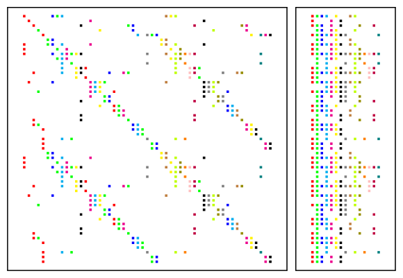
If $n$ becomes larger (>>1000), however, the memory requirement of all $n$ tangents may exceed the GPU’s memory. Since our Jacobian is sparse, we apply the technique of Jacobian coloring that compresses independent columns of the Jacobian and reduces the number of required seeding tangent vectors from $n$ to the number of colors $c$ (see Figure 2).

Figure 2: Jacobian compression via column coloring. On the left, the original Jacobian. On the right, the compressed Jacobian.

4.2.3 Second-Order Derivatives.

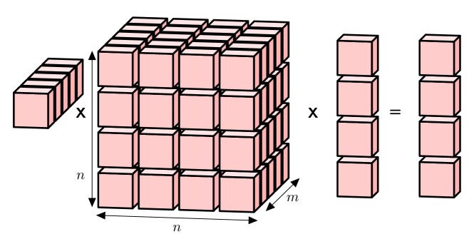
For higher-order derivatives that involve derivative tensors (e.g., Hessian $\nabla^{2}g\in\mathbb{R}^{m\times n\times n}$) we introduce the projection notation $<\cdots>$ introduced in [21] and illustrated in Figure 3 with $<\bm{x}_{(1)},\nabla^{2}g(\bm{x}),\bm{x}^{(1)}>$, whereby adjoints are projected from the left to the Jacobian and tangents from the right. To compute second-order derivatives and the Hessian projections in Equation (4.12), we use the adjoint model implementation given by

(4.13) $$\bm{y}=g(\bm{x}),\ \bm{x}_{(1)}=<\bm{y}^{(1)},\nabla g(\bm{x})>=\bm{y}_{(1)}\cdot\nabla g(\bm{x})^{T}\,,$$

and we apply over it the tangent model given by

(4.14) $$\begin{array}[]{llll}\bm{y}=g(\bm{x}),&\bm{y}^{(1)}=<\nabla g(\bm{x}),\bm{x}^{(1)}>=\nabla g(\bm{x})\cdot\bm{x}^{(1)}\,,\end{array}$$

yielding

(4.15) $$\begin{array}[]{llll}\bm{y}&=g(\bm{x}),\\ \bm{y}^{(2)}&=<\nabla g(\bm{x}),\bm{x}^{(2)}>,\\ \text{and}\\ \bm{x}_{(1)}&=<\bm{y}_{(1)},\nabla g(\bm{x})>,\\ \bm{x}^{(2)}_{(1)}&=<\bm{y}_{(1)},\nabla^{2}g(\bm{x}),\bm{x}^{(2)}>+<\bm{y}^{(2)}_{(1)},\nabla g(\bm{x})>\,.\end{array}$$

Notice that every variable has now a value component and three derivative components denoted by ₍₁₎, ⁽²⁾, and ${}^{(2)}_{(1)}$ amounting to first-order adjoint, second-order tangent, and second-order tangent over adjoint, respectively. In Section 4.3, we compute the term $x_{(1)}^{(2)}$ on the GPU by setting $\bm{y}_{(1)}^{(2)}=0$ and extracting the result from $\bm{x}_{(1)}^{(2)}\in\mathbb{R}^{n}$.

Figure 3: Hessian derivative tensor projection $<\bm{y}_{(1)},\nabla^{2}g(\bm{x}),\bm{x}^{(2)}>$. Notice that the Hessian slices along the $n$ directions are symmetric.

4.3 Reduction Algorithm.

We are now able to write down the reduction algorithm to compute the Hessian-vector products $\nabla^{2}F\cdot\bm{w}$. We first present a sequential version of the algorithm, and then detail how to design a parallel variant of the reduction algorithm.

Data: Vector $\bm{w}\in\mathbb{R}^{n_{p}}$

SpMul: $\bm{b}=\big{(}\nabla_{\bm{u}}g\big{)}\bm{w}$ ;

SparseSolve: $(\nabla_{\bm{x}}{g})\bm{z}=-\bm{b}$ ;

TensorProjection: Compute $(\bm{y}_{\bm{x}},\bm{y}_{\bm{p}})$ with (4.12) and $\bm{v}=(\bm{z},\bm{w})$;

SparseSolve: $(\nabla_{\bm{x}}{g})^{\top}\bm{\psi}=-\bm{y}_{\bm{x}}$ ;

MulAdd: $(\nabla^{2}F)\bm{w}=\bm{y}_{\bm{p}}+(\nabla_{\bm{p}}{g})^{\top}\bm{\psi}$ ;

Algorithm 1 Reduction algorithm

4.3.1 Sequential algorithm.

We observe that by default the Hessian reduction algorithm encompasses four sequential steps:

1. SparseSolve: Get the second-order adjoint $\bm{z}$ by solving the first linear system in (4.10).

2. TensorProjection: Define the tangent $\bm{v}:=(\bm{z},\bm{w})$, and evaluate the second-order derivatives using (4.12). TensorProjection returns a vector $\bm{y}=(\bm{y}_{\bm{x}},\bm{y}_{\bm{p}})$, with

   (4.16) $$\left\{\begin{aligned} \bm{y}_{\bm{x}}=&<\bm{\lambda}^{\top},\nabla_{\bm{x}\bm{x}}^{2}g,\bm{z}>+<\bm{\lambda}^{\top},\nabla_{\bm{x}\bm{p}}^{2}g,\bm{w}>+\\ &<\nabla_{\bm{x}\bm{x}}^{2}f,\bm{z}>+<\nabla_{\bm{x}\bm{p}}^{2}f,\bm{w}>\;,\\ \bm{y}_{\bm{p}}=&<\bm{\lambda}^{\top},\nabla_{\bm{p}\bm{x}}^{2}g,\bm{z}>+<\bm{\lambda}^{\top},\nabla_{\bm{p}\bm{p}}^{2}g,\bm{w}>+\\ &<\nabla_{\bm{p}\bm{x}}^{2}f,\bm{z}>+<\nabla_{\bm{p}\bm{p}}^{2}f,\bm{w}>\;,\end{aligned}\right.$$

   with ‘‘$<>$" denoting the derivative tensor projection introduced in Section 4.2.3 (and illustrated in Figure 3).

3. SparseSolve: Get the second-order adjoint $\bm{\psi}$ by solving the second linear system in Equation (4.10): $(\nabla_{\bm{x}}{g})^{\top}\bm{\psi}=-\bm{y}_{\bm{x}}$.

4. SpMulAdd: Compute the reduced Hessian-vector product with Equation (4.11).

The first SparseSolve differs from the second SparseSolve since the left-hand side is different: the first system considers the Jacobian matrix $(\nabla_{\bm{x}}g)$, whereas the second system considers its transpose $(\nabla_{\bm{x}}g)^{\top}$.

To compute the entire reduced Hessian $\nabla^{2}F$, we have to let $\bm{w}$ go over all the Cartesian basis vectors of $\mathbb{R}^{n_{p}}$. The parallelization over these basis vectors is explained in the next paragraph.

4.3.2 Parallel Algorithm.

Instead of computing the Hessian vector products $(\nabla^{2}F)\bm{w}_{1},\cdots,(\nabla^{2}F)\bm{w}_{n}$ one by one, the parallel algorithm takes as input a batch of $N$ vectors $W=\big{(}\bm{w}_{1},\cdots,\bm{w}_{N}\big{)}$ and evaluates the Hessian-vector products $\big{(}(\nabla^{2}F)\bm{w}_{1},\cdots,(\nabla^{2}F)\bm{w}_{N}\big{)}$ in a parallel fashion. By replacing respectively the SparseSolve and TensorProjection blocks by BatchSparseSolve and BatchTensorProjection, we get the parallel reduction algorithm presented in Algorithm 2 (and illustrated in Figure 4). On the contrary to Algorithm 1, the block BatchSparseSolve solves a sparse linear system with multiple right-hand-sides $B=(\nabla_{\bm{p}}g)W$, and the block BatchTensorProjection runs the Autodiff algorithm introduced in Section 4.2 in batch. As explained in the next section, both operations are fully amenable to the GPU.

Data: $N$ vectors $\bm{w}_{1},\cdots,\bm{w}_{N}\in\mathbb{R}^{n_{p}}$

Build $W=(\bm{w}_{1},\cdots,\bm{w}_{N})$ $,W\in\mathbb{R}^{n_{p}\times N}$ ;

SpMul: $B=\big{(}\nabla_{\bm{p}}g\big{)}W$ $,B\in\mathbb{R}^{n_{x}\times N}$, $\nabla_{\bm{p}}g\in\mathbb{R}^{n_{x}\times n_{p}}$;

BatchSparseSolve: $(\nabla_{\bm{x}}{g})Z=-B$ ;

BatchTensorProjection: Compute $(Y_{\bm{x}},Y_{\bm{p}})$ with $V=(Z,W)$ ;

BatchSparseSolve: $(\nabla_{\bm{x}}{g})^{\top}\Psi=-Y_{\bm{x}}$ ;

SpMulAdd: $(\nabla^{2}F)\bm{W}=Y_{\bm{p}}+(\nabla_{\bm{p}}{g})^{\top}\Psi$ ;

Algorithm 2 Parallel reduction algorithm

Figure 4: Parallel computation of the reduced Hessian vector products on the GPU

5 GPU Implementation

In the previous section, we have devised a parallel algorithm to compute the reduced Hessian. This algorithm involves two key ingredients, both running in parallel: BatchSparseSolve and BatchTensorProjection. We present in Section 5.1 how to implement BatchTensorProjection on GPU by leveraging the Julia language. Then, we focus on the parallel resolution of BatchSparseSolve in Section 5.2. The final implementation is presented in Section 5.3.

5.1 Batched AutoDiff.

5.1.1 AutoDiff on GPU.

Our implementation attempts to be architecture agnostic, and to this end we rely heavily on the just-in-time compilation capabilities of the Julia language. Julia has two key advantages for us: (i) it implements state-of-the-art automatic differentiation libraries and (ii) its multiple dispatch capability allows to write code in an architecture agnostic way. Combined together, this allows to run AutoDiff on GPU accelerators. On the architecture side we rely on the array abstraction implemented by the package GPUArrays.jl [5] and on the kernel abstraction layer KernelAbstractions.jl. The Julia community provides three GPU backends for these two packages: NVIDIA, AMD, and Intel oneAPI. Currently, CUDA.jl is the most mature package, and we are leveraging this infrastructure to run our code on an x64/PPC CPU and NVIDIA GPU. In the future our solution will be rolled out transparently onto AMD and Intel accelerators with minor code changes.

5.1.2 Forward Evaluation of Sparse Jacobians.

The reduction algorithm in Section 4.3 requires (i) the Jacobian $\nabla_{x}g$ to form the linear system in (4.10) and (ii) the Hessian vector product of $\bm{\lambda}^{\top}\nabla^{2}g$ in (4.16). We use the Julia package ForwardDiff.jl [27] to apply the first-order tangent model (4.14) by instantiating every variable as a dual type defined as T1S{T,C} = ForwardDiff.Dual{T, C}}, where T is the type (double or float) and C is the number of directions that are propagated together in parallel. This allows us to apply AutoDiff both on the CPU and on the GPU in a vectorized fashion, through a simple type change: for instance, Array{TIS{T, C}}(undef, n) instantiates a vector of dual numbers on the CPU, whereas CuArray{TIS{T, C}}(undef, n) does the same on a CUDA GPU. (Julia allows us to write code where all the types are abstracted away). This, combined with KernelAbstractions.jl, allows us to write a portable residual kernel for $g(\bm{x},\bm{p})$ that is both differentiable and architecture agnostic. By setting the number of Jacobian colors $c$ to the parameter C of type T1S{T,C} we leverage the GPUs by propagating the tangents in a SIMD way.

5.1.3 Forward-over-Reverse Hessian Projections.

As opposed to the forward mode, generating efficient adjoint code for GPUs is known to be hard. Indeed, adjoint automatic differentiation implies a reversal of the computational flow, and in the backward pass every read of a variable translates to a write adjoint, and vice versa. The latter is particularly complex for parallelized algorithms, especially as the automatic parallelization of algorithms is hard. For example, an embarrassingly parallel algorithm where each process reads the data of all the input space leads to a challenging race condition in its adjoint. Current state-of-the-art AutoDiff tools use specialized workarounds for certain cases. However, a generalized solution to this problem does not exist. The promising AutoDiff tool Enzyme [19] is able to differentiate CUDA kernels in Julia, but it is currently not able to digest all of our code.

To that end, we hand differentiate our GPU kernels for the forward-over-reverse Hessian projection. We then apply ForwardDiff to these adjoint kernels to extract second-order sensitivities according to the forward-over-reverse model. Notably, our test case (see Section 3.1) involves reversing a graph-based problem (with vertices $V$ and edges $E$). The variables of the equations are defined on the vertices. To adjoin or reverse these kernels, we pre-accumulate the adjoints first on the edges and then on the nodes, thus avoiding a race condition on the nodes. This process yields a fully parallelizable adjoint kernel. Unfortunately, current AutoDiff tools are not capable of detecting such structural properties. Outside the kernels we use a tape (or stack) structure to store the values computed in the forward pass and to reuse them in the reverse (split reversal). The kernels themselves are written in joint reversal, meaning that the forward and reverse passes are implemented in one function evaluation without intermediate storage of variables in a data structure. For a more detailed introduction to writing adjoint code we recommend [14].

5.2 Batched Sparse Linear Algebra.

The block BatchSparseSolve presented in Section 4.3 requires the resolution of two sparse linear systems with multiple right-hand sides, as illustrated in Equation (4.10). This part is critical because in practice a majority of the time is spent inside the linear algebra library in the parallel reduction algorithm. To this end, we have wrapped the library cuSOLVER_RF in Julia to get an efficient LU solver on the GPU. For any sparse matrix $A\in\mathbb{R}^{n\times n}$, the library cuSOLVER_RF takes as input an LU factorization of the matrix $A$ precomputed on the host, and transfers it to the device. cuSOLVER_RF has two key advantages to implement the resolution of the two linear systems in BatchSparseSolve. (i) If a new matrix $\tilde{A}$ needs to be factorized and has the same sparsity pattern as the original matrix $A$, the refactorization routine proceeds directly on the device, without any data transfer with the host (allowing to match the performance of the state-of-the-art CPU sparse library UMFPACK [10]). (ii) Once the LU factorization has been computed, the forward and backward solves for different right-hand sides $\bm{b}_{1},\cdots,\bm{b}_{N}$ can be computed in batch mode.

5.3 Implementation of the Parallel Reduction.

By combining the batch AutoDiff with the batch sparse linear solves of cuSOLVER_RF, we get a fully parallel algorithm to compute the reduced Hessian projection. We compute the reduced Hessian $\nabla^{2}F\in\mathbb{R}^{n_{p}\times n_{p}}$ by blocks of $N$ Hessian-vector products. If we have enough memory to set $N=n_{p}$, we can compute the full reduced Hessian in one batch reduction. Otherwise, we set $N<n_{p}$ and compute the full reduced Hessian in $N_{b}=div(n,N)+1$ batch reductions.

Tuning the number of batch reductions $N$ is nontrivial and depends on two considerations. How efficient is the parallel scaling when we run the two parallel blocks BatchTensorProjection and BatchSparseSolve? and Are we fitting into the device memory? This second consideration is indeed one of the bottlenecks of the algorithm. In fact, if we look more closely at the memory usage of the parallel reduced Hessian, we observe that the memory grows linearly with the number of batches $N$. First, in the block BatchTensorProjection, we need to duplicate $N$ times the tape used in the reverse accumulation of the Hessian in Section 5.1, leading to memory increase from $\mathcal{O}(M_{T})$ to $\mathcal{O}(M_{T}\times N)$, with $M_{T}$ the memory of the tape. The principle is similar in SparseSolve, since the second-order adjoints $\bm{z}$ and $\bm{\psi}$ are also duplicated in batch mode, leading to a memory increase from $\mathcal{O}(2n_{x})$ to $\mathcal{O}(2n_{x}\times N)$. This is a bottleneck on large cases when the number of variables $n_{x}$ is large.

The other bottleneck arises when we combine together the blocks BatchSparseSolve and BatchTensorProjection. Indeed, BatchTensorProjection should wait for the first block BatchSparseSolve to finish its operations. The same issue arises when passing the results of BatchTensorProjection to the second BatchSparseSolve block. As illustrated by Figure 4, we need to add two explicit synchronizations in the algorithm. Allowing the algorithm to run the reduction algorithm in a purely asynchronous fashion would require a tighter integration with cuSOLVER_RF.

6 Numerical experiments

In this section we provide extensive benchmarking results that investigate whether the computation of the reduced Hessian $\nabla^{2}f$ with Algorithm 2 is well suited for SIMD on GPU architectures. As a comparison, we use a CPU implementation based on the sparse LU solver UMFPACK, with iterative refinement disabled (it yields no numerical improvement, however, considerably speeds up the computation). We show that on the largest instances our GPU implementation is 30 times faster than its sequential CPU equivalent and provide a path forward to further improve our implementation. Then, we illustrate that the reduced Hessian computed is effective to track a suboptimal in a real-time setting.

6.1 Experimental Setup

6.1.1 Hardware.

Our workstation Moonshot is provided by Argonne National Laboratory. All the experiments run on a NVIDIA V100 GPU (with 32GB of memory) and CUDA 11.3. The system is equipped with a Xeon Gold 6140, used to run the experiments on the CPU (for comparison). For the software, the workstation works with Ubuntu 18.04, and we use Julia 1.6 for our implementation. We rely on our package KernelAbstractions.jl and GPUArrays.jl to generate parallel GPU code.

All the implementation is open-sourced, and an artifact is provided to reproduce the numerical results.

6.1.2 Benchmark library.

The test data represents various case instances (see Table 1) in the power grid community obtained from the open-source benchmark library PGLIB [3]. The number in the case name indicates the number of buses (graph nodes) $n_{v}$ and the number of lines (graph edges) $n_{e}$ in the power grid: $n_{x}$ is the number of variables, while $n_{p}$ is the number of parameters (which is also equal to the dimension of the reduced Hessian and the parameter space $\mathbb{R}^{n_{p}}$).

Case	$n_{v}$	$n_{e}$	$n_{x}$	$n_{p}$
IEEE118	118	186	181	107
IEEE300	300	411	530	137
PEGASE1354	1,354	1,991	2,447	519
PEGASE2869	2,869	4,582	5,227	1,019
PEGASE9241	9,241	16,049	17,036	2,889
GO30000	30,000	35,393	57,721	4,555

Table 1: Case instances obtained from PGLIB

6.2 Numerical Results

6.2.1 Benchmark reduced Hessian evaluation.

Cases	Dimensions
	$W\in\mathbb{R}^{n_{p}\times N}$	$B\in\mathbb{R}^{n_{x}\times N}$	$\nabla^{2}f\in\mathbb{R}^{n_{p}\times n_{p}}$
IEEE118	$107\times N$	$181\times N$	$107\times 107$
IEEE300	$137\times N$	$530\times N$	$137\times 137$
PEGASE1354	$519\times N$	$2,447\times N$	$519\times 519$
PEGASE2869	$1,019\times N$	$5,227\times N$	$1,019\times 1,019$
PEGASE9241	$17,036\times N$	$17,036\times N$	$2,889\times 2,889$
GO30000	$30,000\times N$	$35,393\times N$	$4,555\times 4,555$

Table 2: Size of key matrices (seed matrix $W$, multiple right-hand sides $B$, and final reduced Hessian $\nabla^{2}F$) for a batch size of $N$. On GO30000, instantiating the three matrices $W,B,\nabla^{2}F$ for $N=256$ already takes 286MB in the GPU memory.

.

For the various problems described in Table 1, we benchmarked the computation of the reduced Hessian $\nabla^{2}F$ for different batch sizes $N$. Each batch computes $N$ columns of the reduced Hessian (which has a fixed size of $n_{p}\times n_{p}$). Hence, the algorithm requires $N_{b}=div(n_{p},N)+1$ number of batches to evaluate the full Hessian.

In Figure 5, we compare on various instances (see Table 2) the reference CPU implementation together with the full reduced Hessian computation $\nabla^{2}F$ on the GPU (with various batch sizes $N$). The figure is displayed in log-log scale, to better illustrate the linear scaling of the algorithm. In addition, we scale the time taken by the algorithm on the GPU by the time taken to compute the full reduced Hessian on the CPU: a value below 1 means that the GPU is faster than the CPU.

We observe that the larger the number of batches $N$, the faster the GPU implementation is. This proves that the GPU is effective at parallelizing the reduction algorithm, with a scaling almost linear when the number of batches is small ($N<32=2^{5}$). However, we reach the scalability limit of the GPU as we increase the number of batches $N$ (generally, when $N\geq 256=2^{8}$). Comparing to the CPU implementation, the speed-up is not large on small instances ($\approx$ 2 for IEEE118 and IEEE300), but we get up to a 30 times speed-up on the largest instance GO30000, when using a large number of batches.

Figure 5: Parallel scaling of the total reduced Hessian accumulation $\nabla^{2}F$ with batch size $N$: A ratio value $<1$ indicates a faster runtime compared with that of UMFPACK and AutoDiff on the CPU in absolute time. The dotted lines indicate the linear scaling reference. Lower values imply a higher computational intensity.

Figure 6: Decomposition of the runtime against the number of batch $N$, on case PEGASE 9241. $N=1$ corresponds to the CPU implementation. The derivative computation is the dominant kernel.

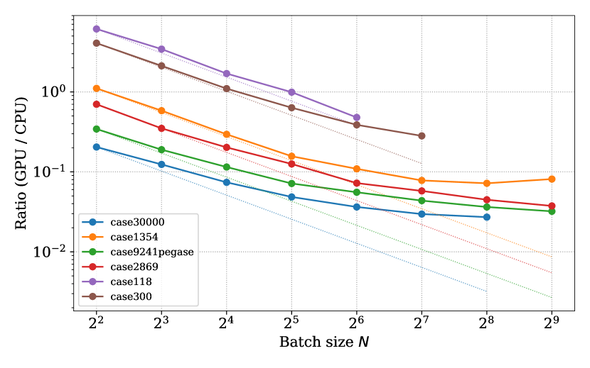
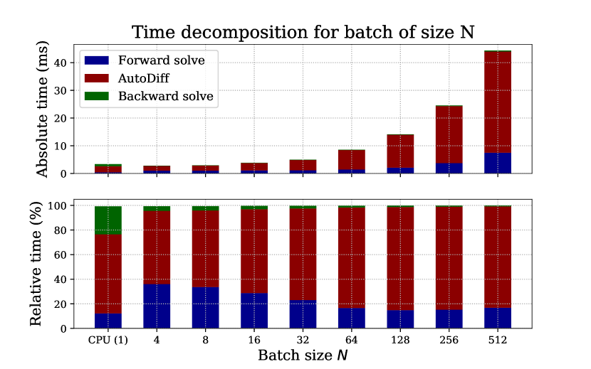
Figure 6 shows the relative time spent in the linear algebra and the automatic differentiation backend. On the CPU, we observe that UMFPACK is very efficient to perform the linear solves (once the iterative refinement is deactivated). However, a significant amount of the total running time is spent inside the AutoDiff kernel. We get a similar behavior on the GPU: the batched automatic differentiation backend leads to a smaller speed-up than the linear solves, increasing the fraction of the total runtime spent in the block BatchAutoDiff.

6.2.2 Discussion.

Our analysis shows that the reduced Hessian scales with the batch size, while hitting an utilization limit for larger test cases. Our kernels may still have potential for improvement, thus further improving utilization scaling as long as we do not hit the memory capacity limit. However, the sparsity of the power flow problems represents a worst-case problem for SIMD architectures, common in graph-structured applications. Indeed, in contrast to PDE-structured problems, graphs are difficult to handle in SIMD architectures because of their unstructured sparsity patterns.

6.3 Real-time tracking algorithm.

Finally, we illustrate the benefits of our reduced Hessian algorithm by embedding it in a real-time tracking algorithm.

Let $\bm{w}_{t}=(\bm{P}^{d}_{t},\bm{Q}_{t}^{d})$ be the loads in (3.3), indexed by time $t$ and updated every minute. In that setting, the reduced space problem is parameterized by the loads $\bm{w}_{t}$:

(6.17) $$\min_{\bm{p}_{t}}\;F(\bm{p}_{t};\bm{w}_{t}):=f\big{(}x(\bm{p}_{t}),\bm{p}_{t};\bm{w}_{t}\big{)}\;.$$

For all time $t$, the real-time algorithm aims at tracking the optimal solutions $\bm{p}_{t}^{\star}$ associated with the sequence of problems (6.17). To achieve this, we update the tracking point $\bm{p}_{t}$ at every minute, by exploiting the curvature information provided by the reduced Hessian. The procedure is the following:

• Step 1: For new loads $\bm{w}_{t}=(\bm{P}_{t}^{d},\bm{Q}_{t}^{d})$, compute the reduced gradient $\bm{g}_{t}=\nabla_{\bm{p}}F(\bm{p}_{t};\bm{w}_{t})$ and the reduced Hessian $H_{t}=\nabla^{2}_{\bm{p}\bm{p}}F(\bm{p}_{t};\bm{w}_{t})$ using Algorithm 2.

• Step 2: Update the tracking control $\bm{p}_{t}$ with $\bm{p}_{t+1}=\bm{p}_{t}+\bm{d}_{t}$, where $\bm{d}_{t}$ is a descent direction computed as solution of the dense linear system

  (6.18) $$H_{t}\;\bm{d}_{t}=-\bm{g}_{t}\;.$$

In practice, we use the dense Cholesky factorization implemented in cuSOLVER to solve the dense linear system (6.18) efficiently on the GPU.

We compare the tracking controls $\{\bm{p}_{t}\}_{t=1,\cdots,T}$ with the optimal solutions $\{\bm{p}_{t}^{\star}\}_{t=1,\cdots,T}$ associated to the sequence of optimization problems (6.17). Note that solving each (6.17) to optimality is an expensive operation, involving calling a nonlinear optimization solver. On the contrary, the real-time tracking algorithm involves only (i) updating the gradient and the Hessian for the new loads $\bm{w}_{t}$ and (ii) solving the dense linear system (6.18).

Figure 7: Performance of the real-time tracking algorithm on PEGASE1354, compared with the optimal solutions. The real-time algorithm is applied every minute, during one hour. The first plot shows the evolution of the operating cost along time, whereas the second plot shows the evolution of the absolute difference between the tracking control $\bm{p}_{t}$ and the optimum $\bm{p}_{t}^{\star}$.

We depict in Figure 7 the performance of the real-time tracking algorithm, compared with an optimal solution computed by a nonlinear optimization solver. In the first subplot, we observe that the operating cost associated to $\{\bm{p}_{t}\}_{t}$ is close to the optimal cost associated to $\{\bm{p}_{t}^{\star}\}_{t}$. The second subplot depicts the evolution of the absolute difference $|\bm{p}_{t}-\bm{p}_{t}^{\star}|$, component by component. We observe that the difference remains tractable: the median (Quantile 50%) is almost constant, and close to $10^{-2}$ (which in our case is not a large deviation from the optimum) whereas the maximum difference remains below $0.5$. At each time $t$, the real-time algorithm takes in average $0.10$s to update $\bm{p}_{t}$ on the GPU (with $N=256$ batches), comparing to $2.22$s on the CPU (see Table 3). We achieve such a 20 times speed-up on the GPU as (i) the evaluation of the reduced Hessian is faster on the GPU (ii) we do not have any data transfer between the host and the device to perform the dense Cholesky factorization with cusolver. Hence, this real-time use case leverages the high parallelism of our algorithm to evaluate the reduced Hessian.

	Step 1 (s)	Step 2 (s)	Total (s)
CPU	1.41	0.81	2.22
GPU	0.05	0.05	0.10

Table 3: Time to update the tracking point $\bm{p}_{t}$ for case1354pegase with the real-time algorithm, on the CPU and on the GPU.

7 Conclusion

In this paper we have devised and implemented a practical batched algorithm (see Algorithm 2) to extract on SIMD architectures the second-order sensitivities from a system of nonlinear equations. Our implementation on NVIDIA GPUs leverages the programming language Julia to generate portable kernels and differentiated code. We have observed that on the largest cases the batch code is 30x faster than a reference CPU implementation using UMFPACK. This is important for upcoming large-scale computer systems where availability of general purpose CPUs is very limited. We have illustrated the interest of the reduced Hessian when used inside a real-time tracking algorithm. Our solution adheres to the paradigm of differential and composable programming, leveraging the built-in metaprogramming capabilities of Julia. In the future, we will investigate extending the method to other classes of problems (such as uncertainty quantification, optimal control, trajectory optimization, or PDE-constrained optimization).

The submitted manuscript has been created by UChicago Argonne, LLC, Operator of Argonne National Laboratory (‘‘Argonne"). Argonne, a U.S. Department of Energy Office of Science laboratory, is operated under Contract No. DE-AC02-06CH11357. The U.S. Government retains for itself, and others acting on its behalf, a paid-up nonexclusive, irrevocable worldwide license in said article to reproduce, prepare derivative works, distribute copies to the public, and perform publicly and display publicly, by or on behalf of the Government. The Department of Energy will provide public access to these results of federally sponsored research in accordance with the DOE Public Access Plan. http://energy.gov/downloads/doe-public-access-plan.

References

- [1] M. Abadi, A. Agarwal, P. Barham, E. Brevdo, Z. Chen, C. Citro, G. S. Corrado, A. Davis, J. Dean, M. Devin, S. Ghemawat, I. Goodfellow, A. Harp, G. Irving, M. Isard, Y. Jia, R. Jozefowicz, L. Kaiser, M. Kudlur, J. Levenberg, D. Mané, R. Monga, S. Moore, D. Murray, C. Olah, M. Schuster, J. Shlens, B. Steiner, I. Sutskever, K. Talwar, P. Tucker, V. Vanhoucke, V. Vasudevan, F. Viégas, O. Vinyals, P. Warden, M. Wattenberg, M. Wicke, Y. Yu, and X. Zheng. TensorFlow: Large-scale machine learning on heterogeneous systems, 2015.
- [2] A. Ahmadi, S. Jin, M. C. Smith, E. R. Collins, and A. Goudarzi. Parallel power flow based on openmp. In 2018 North American Power Symposium (NAPS), pages 1--6. IEEE, 2018.
- [3] S. Babaeinejadsarookolaee, A. Birchfield, R. D. Christie, C. Coffrin, C. DeMarco, R. Diao, M. Ferris, S. Fliscounakis, S. Greene, R. Huang, et al. The power grid library for benchmarking AC optimal power flow algorithms. arXiv preprint arXiv:1908.02788, 2019.
- [4] L. Beda et al. Programs for automatic differentiation for the machine besm. Precise Mechanics and Computation Techniques, Academy of Science, Moscow, 1959.
- [5] T. Besard, C. Foket, and B. De Sutter. Effective extensible programming: unleashing Julia on GPUs. IEEE Transactions on Parallel and Distributed Systems, 30(4):827--841, 2018.
- [6] J. Bezanson, A. Edelman, S. Karpinski, and V. B. Shah. Julia: A fresh approach to numerical computing. SIAM Rev., 59(1):65--98, 2017.
- [7] L. T. Biegler, O. Ghattas, M. Heinkenschloss, and B. van Bloemen Waanders. Large-scale PDE-constrained optimization: an introduction. In Large-Scale PDE-Constrained Optimization, pages 3--13. Springer, 2003.
- [8] J. Blühdorn, N. R. Gauger, and M. Kabel. AutoMat -- automatic differentiation for generalized standard materials on gpus. arXiv preprint arXiv:2006.04391, 2020.
- [9] A. E. Bryson and W. F. Denham. A steepest-ascent method for solving optimum programming problems. Journal of Applied Mechanics, 29:247, 1962.
- [10] T. A. Davis. Algorithm 832: UMFPACK v4.3---an unsymmetric-pattern multifrontal method. ACM Trans. Math. Software, 30(2):196--199, 2004.
- [11] H. W. Dommel and W. F. Tinney. Optimal power flow solutions. IEEE Transactions on power apparatus and systems, (10):1866--1876, 1968.
- [12] J. C. Gilbert. Automatic differentiation and iterative processes. Optimization methods and software, 1(1):13--21, 1992.
- [13] M. Grabner, T. Pock, T. Gross, and B. Kainz. Automatic differentiation for GPU-accelerated 2d/3d registration. In Advances in automatic differentiation, pages 259--269. Springer, 2008.
- [14] A. Griewank and A. Walther. Evaluating derivatives: principles and techniques of algorithmic differentiation. SIAM, 2008.
- [15] J. C. Hückelheim, P. D. Hovland, M. M. Strout, and J.-D. Müller. Parallelizable adjoint stencil computations using transposed forward-mode algorithmic differentiation. Optimization Methods and Software, 33(4-6):672--693, 2018.
- [16] M. Innes. Flux: Elegant machine learning with julia. Journal of Open Source Software, 3(25):602, 2018.
- [17] J. Kardos, D. Kourounis, and O. Schenk. Reduced-space interior point methods in power grid problems. arXiv preprint arXiv:2001.10815, 2020.
- [18] S. Linnainmaa. Taylor expansion of the accumulated rounding error. BIT Numer. Math., 16(2):146--160, 1976.
- [19] W. S. Moses and V. Churavy. Instead of rewriting foreign code for machine learning, automatically synthesize fast gradients. In Advances in Neural Information Processing Systems, volume 33, pages 12472--12485. 2020.
- [20] W. S. Moses, V. Churavy, L. Paehler, J. Hückelheim, S. H. K. Narayanan, M. Schanen, and J. Doerfert. Reverse-mode automatic differentiation and optimization of GPU kernels via Enzyme. In Proceedings of the International Conference for High Performance Computing, Networking, Storage and Analysis, SC ’21, New York, NY, USA, 2021. Association for Computing Machinery.
- [21] U. Naumann. The Art of Differentiating Computer Programs: An Introduction to Algorithmic Differentiation. SIAM, 2012.
- [22] J. F. Nolan. Analytical differentiation on a digital computer. PhD thesis, Massachusetts Institute of Technology, 1953.
- [23] D. Papadimitriou and K. Giannakoglou. Direct, adjoint and mixed approaches for the computation of hessian in airfoil design problems. International journal for numerical methods in fluids, 56(10):1929--1943, 2008.
- [24] A. Paszke et al. PyTorch: An imperative style, high-performance deep learning library. In Advances in Neural Information Processing Systems 32, pages 8024--8035. Curran Associates, Inc., 2019.
- [25] B. A. Pearlmutter. Fast exact multiplication by the hessian. Neural computation, 6(1):147--160, 1994.
- [26] J. Revels, T. Besard, V. Churavy, B. D. Sutter, and J. P. Vielma. Dynamic automatic differentiation of GPU broadcast kernels. CoRR, abs/1810.08297, 2018.
- [27] J. Revels, M. Lubin, and T. Papamarkou. Forward-mode automatic differentiation in Julia. arXiv preprint arXiv:1607.07892, 2016.
- [28] Y. Tang, K. Dvijotham, and S. Low. Real-time optimal power flow. IEEE Transactions on Smart Grid, 8(6):2963--2973, 2017.
- [29] W. F. Tinney and C. E. Hart. Power flow solution by Newton’s method. IEEE Transactions on Power Apparatus and systems, (11):1449--1460, 1967.
- [30] Z. Wang, S. Wende-von Berg, and M. Braun. Fast parallel Newton–Raphson power flow solver for large number of system calculations with CPU and GPU. Sustainable Energy, Grids and Networks, 27:100483, Sep 2021.