Asymptotic Experiments with Data Structures:
Bipartite Graph Matchings and Covers

Abstract

We consider instances of bipartite graphs and a number of asymptotic performance experiments in three projects: (1) top movie lists, (2) maximum matchings, and (3) minimum set covers. Experiments are designed to measure the asymptotic runtime performance of abstract data types (ADTs) in three programming languages: Java, R, and C++. The outcomes of these experiments may be surprising. In project (1), the best ADT in R consistently outperforms all ADTs in public domain Java libraries, including the library from Google. The largest movie list has $2^{20}$ titles. In project (2), the Ford-Fulkerson algorithm implementation in R significantly outperforms Java. The hardest instance has 88452 rows and 729 columns. In project (3), a stochastic version of a greedy algorithm in R can significantly outperform a state-of-the-art stochastic solver in C++ on instances with $num\_rows\geq 300$ and $num\_columns\geq 3000$.

1 Introduction

The title of this article was by inspired by a 2-sentence abstract from a 92-page publication [1]: “Almost all combinatorial questions can be reformulated as either a matching or a covering problem of a hypergraph. In this paper we survey some of the important results.”.

Rather than theorems and proofs, this article is about asymptotic performance experiments on matching and covering problems with data structures that represent the hypergraph as a bipartite graph: a matrix with $m$ rows and $n$ columns. For an illustration of matching and covering problems addressed in this article, see the example of the 11-row, 9-column bigraph in Section 3, Figure 4.

Companion articles [2, 3] provide the background and the motivation for a series of experiments we report in four sections of this article:

Beyond CSC316 and Java

Data structures impact the asymptotic runtime performance when creating lists such as the top 10 most frequently watched movies. The key finding is that the data.table structure in R [4] significantly outperforms all of the best-known and widely available ADTs in Java. The largest movie list has $2^{20}$ titles.

Maximum Matching in Bipartite Graphs

We compare runtime performance of two public-domain implementations of the Ford-Fulkerson algorithm: Java and R. The hardest instance has 88452 rows and 729 columns. Again, R significantly outperforms the implementation in Java.

Greedy Heuristic Distributions for Set Cover

The importance of greedy heuristics is increasing as the instance sizes increase for problems such as the minimum set cover. We demonstrate that a stochastic version of a greedy algorithm in R can significantly outperform a state-of-the-art stochastic solver in C++ on instances with $num\_rows\geq 300$ and $num\_columns\geq 3000$.

Future Work

The work in progress includes extensions of new heuristics, outlined in the companion article [3], to a number of hard combinatorial optimization problems.

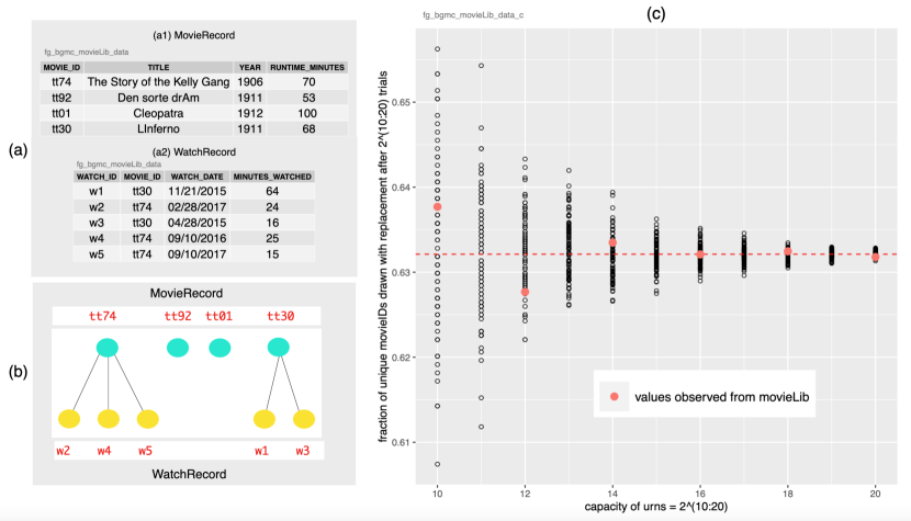
Figure 1: Representations of data sets used in the performance experiments with the MovieLib data set introduced in Section 2: (a) a tabular organization of files MovieRecord and WatchRecord, (b) a bigraph that illustrates relationships between the items from the two files in (a), and (c) a statistical model, based on $2^{10}~{}...~{}2^{20}$ trials of sampling with replacement from 11 urns, each with urn capacity of holding $2^{10}~{}...~{}2^{20}$ unique movieID tags. The actual MovieLib is represented with 6 urns: their sizes are $2^{10}$, $2^{12}$, $2^{14}$, $2^{16}$, $2^{18}$, and $2^{10}$. Notably, the fraction of unique movieID tags observed by analyzing actual data from MovieLib is also converging towards $1-e^{-1}=0.6321$ and is well within the expected range for this experiment.

2 Beyond CSC316 and Java

CSC316 is a junior-level course in data structures and algorithms [5]. A class project relevant to this article, PackFlix, explored the impact of data structures on runtime performance. The data for PackFlix, modified for educational purposes, originated with IMDb [6]. The project objective was to not only analyze the watching histories of customers by designing a software prototype PackFlix in Java. The primary objective was to study the impact of data structures on the asymptotic runtime performance to create lists such as the top 10 most frequently watched movies. The primary input to PackFlix is a directory path to movieLib which contains file pairs of increasing size: movieRecords and watchRecords.

The example in Figure 1 illustrates the organization of two data files and the range of file sizes that are being considered for the experiments.

Two tables in Figure 1a, MovieRecord and WatchRecord are related. Columns in the first table refer to a unique movieID, a title, a release year, and runtime in minutes. Columns in the second table refer to a watchID, movieID, a watch date, and minutes watched.

The Figure 1b is a bipartite graph (a bigraph) that illustrates relationships between the items from the two files in Figure 1a. The movie tt74 has been watched 3 times, the movie tt30 has been watched once, and the remaining two movies have not been watched. Clearly, the most popular movie is tt74.

The Figure 1c depicts experiments with a series of urn models [7], based on $2^{10}~{}...~{}2^{20}$ trials of sampling with replacement from 11 urns, each holding $2^{10}~{}...~{}2^{20}$ unique movieID tags. The experiments are structured to measure the ratio of unique movieID tags observed after $2^{10}~{}...~{}2^{20}$ trials. As the size of urns and the number of trials increases, this ratio converges to the value of $1-e^{-1}=0.6321$. The movies that are actually catalogued in MovieLib are represented as six urns: their sizes are $2^{10}$, $2^{12}$, $2^{14}$, $2^{16}$, $2^{18}$, and $2^{20}$. Notably, both the models and the analysis of actual data from MovieLib converge to the expected value of $1-e^{-1}=0.6321$.

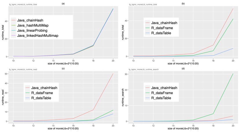
Figure 2: Asymptotic runtime performance experiments with instances from movieLib, based on Java and R code. In each case, the objective is to retrieve the top 10 movies after reading two sets of files: one listing movies and one listing viewer interactions with each movie. In (a), we report runtime_total for best four data structures in Java; a model used in CSC316 class. In (b), we report on runtime_total for the single best data structure in Java (c͡hainHash) in comparison with two best data structures in R (d͡ataFrame and d͡ataTable). In (c), we report runtime_read for chainHash in Java and dataFrame and dataTable in R. In (d), we report runtime_search for chainHash in Java and dataFrame and dataTable in R. There is no doubt that, for instances from movieLib, R significantly outperforms Java – with dataTable an asymptotically better data structure in comparison with dataFrame.

2.1 Data Structures and Java Libraries

Data structures introduced in CSC316 are standard Java libraries introducing a number of Java ADTs, from Linked List to Linear Probing Hash Map.

In this article, we extend our runtime performance experiments to additional Java ADTs: Hash MultiMap and Linked Hash MultiMap from Google Guava [8] and Chain Hash Map from net.datastructures, posted at the Brown University [9].

The Java code uses Map ADT to pair each key and value. Initially, our R code also paired each key with a value using a hash function. However, the runtime performance was worse than Java ADT. This led to exploration of two data structures in R: data.frame [10] and data.table [11]. The Eureka moment came with the observation that data.table in R significantly outperforms the best Java version. For details, see Figure 2.

2.2 Runtime experiments: Java vs R

The four plots in Figure 2, illustrate the runtime performance for PackFlix in Java and R. In the previous section, we introduced four Map ADTs in Java, which are from course work and public domain.

Plot in Figure 2a

is a repeat of experiments in CSC316: it depicts runtime_total of PackFlix with the Map ADTs from Java. Results show that these runtimes are statistically equivalent. For the follow-up experiments in Figures 2b,c,d we select Java_chainHash as a representative of the best Java ADTs to be compared with the two ADTs in R.

Plot in Figure 2b

depicts runtime_total of PackFlix with Java_chainHash, R_dataFrame, and R_dataTable. Here, we observe that runtime_read of PackFlix under Java is significantly outperformed by both ADTs in R. Questions that arise are these:
(1) Which ADT is the best when reading files and initializing the respective data structures?
(2) Which ADT is the best when searching the dataset before returning the top 10 movies?

Plot in Figure 2c

depicts only the runtime_read of PackFlix with Java_chainHash, R_dataFrame, and R_dataTable. Again, we observe that runtime_read of PackFlix under Java is significantly outperformed by both ADTs in R. In principle, Java can read large datasets efficiently. However, in PackFlix, it not only needs to read line by line from each data files, but it also needs to convert each line of data into objects and save them into a global array. This appears as the major factor that Java programs in PackFlix cannot compete with ADTs in R. This question best left to R developers: why does R_dataTable, under runtime_read, start to outperform R_dataFrame at instance sizes $\geq 2^{18}$?

Plot in Figure 2d

focuses on the runtime_search of PackFlix with Java_chainHash, R_dataFrame, and R_dataTable. All of these programs return the same list of the top 10 most frequently watched movies. However, there are significant differences in the runtime_search for the largest movie list with $2^{20}$ titles. Again, R_dataTable significantly outperforms Java_chainHash. But here, Java_chainHash significantly outperforms R_dataFrame. Another question for developers of R: why does the gap in runtime_search between R_dataFrame and R_dataTable increases so rapidly for this dataset?

2.3 Correlation Experiments with MovieLib Dataset

We complete the analysis of experiments with PackFlix and the MovieLib dataset by a frequency analysis of the top 10 movie watched and the total number of movies watched for the largest movie list with $2^{20}$ titles.

Plot in Figure 3a

depicts the frequency of top 10 movies watched. The movie with index 1 has been watched 9 times, movies with indices 2-9 have been watched 8 times, etc.

Plot in Figure 3b

counts the total number of movies watched: 385,128 movies have been watched only once (index = 1), 75 movies have been watched 7 times (index = 7), only one movie has been watched 9 times (index = 9).

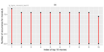
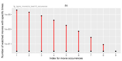
Figure 3: These two plots relate results for the largest movie list with $2^{20}$ titles. The plot (a) depicts the frequency of top 10 movies watched. For example, the movie with index 1 has been watched 9 times, movies with indices 2-9 have been watched 8 times, etc.
The plot (b) counts the total number of movies watched. For example, 385128 movies have been watched only once (index = 1), 75 movies have been watched 7 times (index = 7), only one movie has been watched 9 times (index = 9).

3 Maximum Matching in Bipartite Graphs

Given a graph $G=(V,E)$, a matching M in G is a set of pairwise non-adjacent edges. A maximum matching, also known as maximum-cardinality matching, is a matching that contains the largest possible number of edges. Every maximum matching is maximal, but not every maximal matching is a maximum matching.

Versions of maximum matching problems arise in a number of contexts and applications: from flow and neural networks, scheduling and planning, modeling bonds in chemistry, graph coloring, the stable marriage problem, to matching kidney donors to kidney donor recipients, etc.

The 59-page chapter on maximum-flow problem formulations in [12] includes a section on the maximum bipartite matching. Maximum matching runtime in an undirected bipartite graph $G=(V,E)$ ranges from polynomial in $|V|$ and $|E|$ with the Ford-Fulkerson method [13] to $O(\sqrt{(}|V|)|E|)$ with the Hopcroft and Karp algorithm [14].

Computational experiments with maximum bipartite matching in this article are conducted with two solvers that both rely on Ford-Fulkerson method: one implemented in Java [15], the other implemented in R [16].

The bigraph instances in these experiments are the same ones we use for the experiments in the next section where we search for the minimum set cover. The instances have been assembled as larger instance subsets from variety of sources: the subset of steiner3 instances [17], the subset of OR-library instances [18], and the subset of logic optimization instances [19]. We converted all files to the DIMACS cnf format [20] with minor extensions. This format unifies the formulations of both the minimum unate as well as the minimum binate covering problems [21]. The file extension .cnfU implies a unate set instance with unit weights, the file extension .cnfW implies a unate or a binate set instance with non-unit weights.

Table 1: This table supports discussions in Section 3 as well as in Section 4. Columns denote the name of the instance file, number of instance columns (nCols), number of instance rows (mRows), matrix density column (mDens $:=$ numEdges$/$(nCols*mRows)), maximum matrix degree column (mCD), a column with relative values of maximum matchings for each instance, (mP $:=$ max_matchingSize$/$nCols), best-known-values of the minimum set cover (BKV), Chvatal’s upper bound on the minimum set cover (UB), observed set cover statistics with the Chvatal’s greedy algorithm (value_Chvatal_stats), and set cover statistics normalized with BKV, (BKV_ratio_stats). Instance file name extensions, .cnfU and .cnfW, denote instances with unit weighted columns and pre-assigned weighted columns, respectively. The reported statistics represents values of minimum, median, mean, standard deviation, and maximum. Except for instances that are prefixed with **, the reported statistics are based on experiments with 1000 replications. Experiments with six instances prefixed with ** are based on 10,000 replications.

instance	nCols	mRows	mDens	mCD	mP	BKV	UB	value_Chvatal_stats	BKV_ratio_stats
steiner3
s3_027_117.cnfU	27	117	0.1111	13	1.00	18	57.24	19,19,19,0,19	1.06,1.06,1.06,0.00,1.06
s3_045_330.cnfU	45	330	0.0667	22	1.00	30	110.72	31,32,31.87,0.9,33	1.03,1.07,1.06,0.03,1.10
s3_081_1080.cnfU	81	1080	0.0370	40	1.00	61	260.99	65,65,65,0,65	1.07,1.07,1.07,0.00,1.07
s3_135_3015.cnfU	135	3015	0.0222	67	1.00	103	493.3	107,107,107.92,1.35,111	1.04,1.04,1.05,0.01,1.08
s3_243_9801.cnfU	243	9801	0.0123	121	1.00	198	1064.67	211,211,211,0,211	1.07,1.07,1.07,0.00,1.07
s3_405_27270.cnfU	405	27270	0.0074	202	1.00	335	1972.47	349,350,350.75,2.02,357	1.04,1.04,1.05,0.01,1.07
s3_729_88452.cnfU	729	88452	0.0041	364	1.00	617	3995.53	665,665,665,0,665	1.08,1.08,1.08,0.00,1.08
orlib
$**$scpb1.cnfU	3000	300	0.0499	29	0.10	22	87.16	22,24,23.93,0.5,25	1.00,1.09,1.09,0.02,1.14
$**$scpc1.cnfU	4000	400	0.0200	21	0.10	44	160.4	44,47,46.86,0.82,50	1.00,1.07,1.06,0.02,1.14
$**$scpd1.cnfU	4000	400	0.0501	39	0.10	25	106.34	25,27,26.67,0.48,28	1.00,1.08,1.07,0.02,1.12
$**$scpb1.cnfW	3000	300	0.0499	29	0.10	69	273.35	72,76,75.73,2.06,85	1.04,1.10,1.10,0.03,1.23
$**$scpc1.cnfW	4000	400	0.0200	21	0.10	227	827.5	249,257,256.67,2.83,265	1.10,1.13,1.13,0.01,1.17
$**$scpd1.cnfW	4000	400	0.0501	39	0.10	60	255.21	66,71,70.9,1.66,78	1.10,1.18,1.18,0.03,1.30
scp41.cnfW	1000	200	0.0200	11	0.20	429	1295.53	461,463,466.94,5.1,473	1.07,1.08,1.09,0.01,1.10
scp42.cnfW	1000	200	0.0199	10	0.20	512	1499.63	568,580,582.46,9.85,612	1.11,1.13,1.14,0.02,1.20
scp43.cnfW	1000	200	0.0199	11	0.20	516	1558.26	589,591,592.85,3.62,598	1.14,1.15,1.15,0.01,1.16
scp44.cnfW	1000	200	0.0200	10	0.20	494	1446.91	540,547,547.8,4.18,555	1.09,1.11,1.11,0.01,1.12
scp45.cnfW	1000	200	0.0197	11	0.20	512	1546.18	571,577,574,3,577	1.12,1.13,1.12,0.01,1.13
scp46.cnfW	1000	200	0.0204	10	0.20	560	1640.22	603,612,611.6,5.12,620	1.08,1.09,1.09,0.01,1.11
scp47.cnfW	1000	200	0.0196	12	0.20	430	1334.38	474,474,474.96,1,476	1.10,1.10,1.10,0.00,1.11
scp48.cnfW	1000	200	0.0201	10	0.20	492	1441.05	521,538,538.29,8.93,557	1.06,1.09,1.09,0.02,1.13
scp49.cnfW	1000	200	0.0198	11	0.20	641	1935.74	741,747,745.5,3.33,750	1.16,1.17,1.16,0.01,1.17
scp51.cnfW	2000	200	0.0200	10	0.10	253	741.03	282,291,290.33,2.28,295	1.11,1.15,1.15,0.01,1.17
scp61.cnfW	1000	200	0.0492	20	0.20	138	496.49	152,157,157.1,2.01,163	1.10,1.14,1.14,0.01,1.18
scpa1.cnfW	3000	300	0.0201	17	0.10	253	870.21	273,286,286.03,4.68,297	1.08,1.13,1.13,0.02,1.17
random
m100_50_10_10.cnfU	50	100	0.2000	31	1.00	8	32.22	8,8,8.35,0.48,9	1.00,1.00,1.04,0.06,1.12
m100_100_10_10.cnfU	100	100	0.1000	17	1.00	12	41.27	13,14,13.6,0.51,15	1.08,1.17,1.13,0.04,1.25
m100_100_10_15.cnfU	100	100	0.1239	22	1.00	10	36.91	10,11,11.25,0.51,13	1.00,1.10,1.12,0.05,1.30
m100_100_10_30.cnfU	100	100	0.1968	32	1.00	9	36.53	9,10,9.95,0.83,12	1.00,1.11,1.11,0.09,1.33
m100_100_30_30.cnfU	100	100	0.3000	43	1.00	6	26.1	6,6,6,0,6	1.00,1.00,1.00,0.00,1.00
m200_100_10_30.cnfU	100	200	0.1974	51	1.00	11	49.71	11,12,11.98,0.28,13	1.00,1.09,1.09,0.03,1.18
m200_100_30_50.cnfU	100	200	0.3970	99	1.00	6	31.06	6,6,6,0,6	1.00,1.00,1.00,0.00,1.00
tiny
chvatal_6_5.cnfW	6	5	0.3333	5	0.83	1.1	2.51	2.28,2.28,2.28,0,2.28	2.07,2.07,2.07,0.00,2.07
school_9_11__0.cnfU	9	11	0.2424	3	1.00	4	7.33	4,5,4.85,0.68,6	1.00,1.25,1.21,0.17,1.50
school_9_16.cnfU	9	16	0.2500	6	1.00	5	12.25	6,6,6,0,6	1.20,1.20,1.20,0.00,1.20
school_9_16.cnfW	9	16	0.2500	6	1.00	10	24.5	10,10.5,10.57,0.54,11.5	1.00,1.05,1.06,0.05,1.15
school_19_20.cnfW	19	20	0.1421	6	1.00	11.5	28.18	11.5,13.5,13.39,0.91,15.5	1.00,1.17,1.16,0.08,1.35
instance	nCols	mRows	mDens	mCD	mP	BKV	UB	value_Chvatal_stats	BKV_ratio_stats

Table 1 introduces all instances we use in experiments that evaluate the performance of the maximum matching solvers and the minimum set cover solvers. Columns that characterize each instance, both for the maximum matching problem as well as for the minimum set cover problem include: the number of instance columns (nCols), the number of instance rows (mRows), the matrix density column (mDens $:=$ numEdges$/$(nCols*mRows)), and the maximum matrix degree column (mCD). Only the column mP relates to the maximum matching problem: it denotes the percentage of columns that form the maximum matching (mP $:=$ max_matching$/$nCols). The remainder of columns, starting with the best-known-value of the minimum set cover (BKV), will be explained in next section. All datasets and programs to support replications of results in this paper are available at [22].

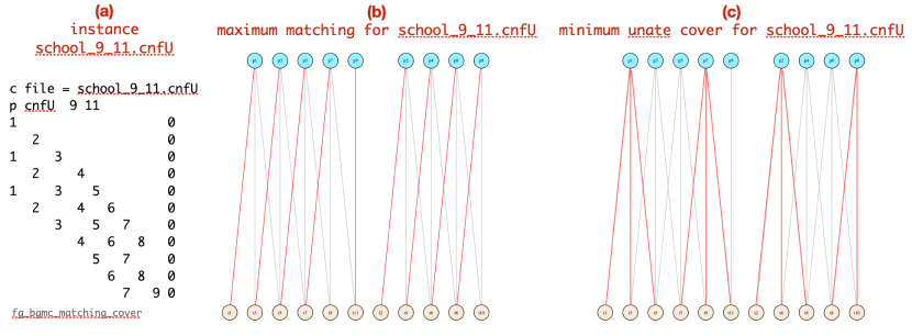
Figure 4: Three views of the instance school_9_11__0.cnfU introduced in Table 1: (a)  an 11-row, 9-column sparse matrix in a cnf format [20], (b)  the maximum bipartite matching problem: with 9 red edges representing the optimum solution, (c)  the minimum set covering problem: 4 vertices at the top cover all 11 vertices at the bottom as illustrated with 11 edges.

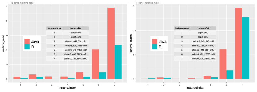
Figure 5: Maximum bipartite matching experiments with three datasets steiner3 [17], orlib [18], and random [19] and two solvers: the solver in Java [15] and the solver in R [16]. The plot on left shows the runtime_read for both solvers. The plot on right shows the runtime_match for both solvers, i.e. the runtime to find the maximum matching. Only instances with runtimes $\geq$ 0.15 seconds are shown.

The example in Figure 4 illustrates three views of the instance school_9_11__0.cnfU introduced in Table 1:

Figure 4a

an 11-row, 9-column matrix in a cnf format [20].

Figure 4b

a bigraph as a two-layered graph that illustrates the maximum matching problem: 11 applicants applying for 1, 2, or 3 of the 9 jobs (teaching positions) advertised by a school. Each job opening can only accept one applicant and a job applicant can be appointed for only one job. In this example, 9 applicants have been matched to 9 jobs: each match is represented by a red-colored edge.

Figure 4c

a bigraph as a two-layered graph illustrates the a unate covering problem: 11 subjects (math, physics, etc) can be taught by 9 instructors. Seven instructors can teach up to 3 subjects, one instructor can teach 2 subjects, one instructor can teach 1 subject only. The objective of the school principal is to hire the minimum number of teachers while still able to offer classes for the 11 subjects. In contrast to the maximum matching problem, the minimum cost solution for this covering problem is not as obvious as it is for the matching problem, even for this small example. There are only two minimum cost solutions: a total of 4 instructors can teach all subjects. The red-colored edges identify 3 instructors who will teach three subjects and 1 instructor will teach two subjects.

The extension of the unate set cover to the binate set cover problem requires addition of binate clauses as additional rows in the sparse matrix configuration. For example, if applicants ’2’ and ’5’ are a married couple, and the school principal would like to hire them both, the matrix in Figure 4a will be extended with these two rows:
                   -2    5
                    2   -5

On the other hand, if applicants ’4’ and ’7’ are a divorced couple, the school principal may prefer to find a minimum cover solution that precludes the hiring of these two individuals together: either ’4’ or ’7’ may be hired but not both. In this case, the matrix in Figure 4a will be extended with this row:
                   -4   -7

3.1 Runtime experiments: Java vs R

Our asymptotic experiments have been performed with two solvers: one implemented in Java [15], the other implemented in R [16]. Both rely on Ford-Fulkerson method [13]. The instances tested by both solvers have been introduced in Table 1. The results are summarized in Figure 5, but only for instances with runtimes $\geq$ 0.15 seconds. Most importantly, we separate the total runtime into two components: (1) runtime to read and set-up all data structures (runtime_read), (2) runtime to find the maximum matching (runtime_match).

runtime_read:

Java is significantly outperformed by R. For the largest instance steiner3_729_88452.cnfU (729 columns, 88452 rows), runtime_read_java $\approx$ 4.9 seconds, runtime_read_R $\approx$ 2.3 seconds. As instance size increases, R gains advantage when using its data.table structure. In contrast, Java may need to scan each line and convert the data into a matrix.

runtime_match:

All except two instances from the subset of OR-library instances, scpb1 and scpd1, are below the runtime threshold of less than 0.15 seconds. While Java is consistently outperformed by R, we would need larger instances to assess whether this trend holds. So far, the increase in runtime_match is monotonically increasing with the decreasing matrix density, both for Java and R. For the largest instance, steiner3_729_88452.cnfU, runtime_match_java $\approx$ 2.9 seconds while runtime_match_R $\approx$ 2.5 seconds.

4 Greedy Heuristic Distributions for Set Cover

Minimum set covering problems arise in a number of domains. In logistics, the context includes market analysis, crew scheduling, emergency services, etc. Electronic design automation deals with logic minimization, technology mapping, and FSM optimization. In bioinformatics, combining Chromatin ImmunoPrecipitation (ChIP) with DNA sequencing to identify the binding sites of DNA-associated proteins leads to formulation of the motif selection problem, mapped to a variant of the set cover problem.

An Integer Linear Programming (ILP) problem formulation guarantees an optimum solution – provided the solver does not time out for large problem instances. The companion article [3] addresses these problems by way of alternative stochastic approaches that go beyond the simple stochastic solver introduced in this section. Our solver is a extension of the greedy set cover algorithm by Chvatal [23, 24]. This version, implemented in R, can significantly outperform a state-of-the-art stochastic solver in C++ for sufficiently large problem instances. The next three sections summarize problem isomorphs, the algorithm implementation, and experimental results.

4.1 On Impact of Problem Isomorphs

The idea of problem isomorphs to design and evaluate learning experiments  [25] is an on-going area of research [26]; it goes back to 1969 as per quote on page 382 [27]:

“I think I invented the idea of problem isomorphs about 1969 or a little earlier … as a follow-up on the AI researcher Saul Amarel’s comment that the representation of the problem could sometimes greatly facilitate its solution …”

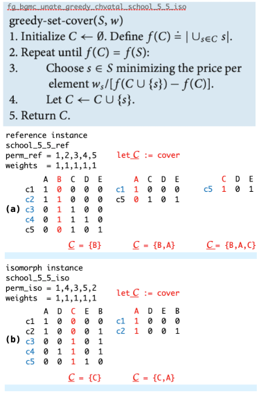
Figure 6: The pseudo code of the greedy algorithm above is from [24]; it represents the version of the Chvatal’s algorithm in [23]. The R-function that implements this algorithm is named unate_greedy_chvatal_basic in Figure 8a. The algorithm is invoked on two instance bigraphs, represented as two incidence matrices: (a) the reference instance school_5_5_ref, and (b) the instance isomorph school_5_5_iso. As implied by the matrix structure, the weight of each column is 1. For (a), the algorithm selects the first column with minimum rate between column weight and column degree, i.e. column B. In the next iteration, there remain only two rows to consider: s1 and s5. The first column with maximum degree is now column A. The algorithm terminates by selecting column C, returning a solution as 3 columns {B, A, C} and the total weight of 3. For (b), the algorithm selects C as the first column with minimum rate between column weight and column degree. The next iteration is also the last. With the selection of column A, we get a solution as 2 columns {C, A} and the total weight of 2.

The isomorphs revisited in this article have a different context and formulation. Their merits, to change the representation of the problem without changing the problem itself, have already been demonstrated by solving instances of combinatorial problems. In the worst case, solvers may timeout for some, but not all, isomorphs before finding the optimum solution [28, 29, 30, 21, 31].

The pseudo code of the greedy algorithm in Figure 6, is the core for our stochastic algorithm. Two instance isomorphs illustrate the importance of representation when invoking the same greedy algorithm on each of the two instances: we observe two solutions that differ by 50%. A narative that follows provides a simple interpretation on how these two instances could have been created:

Scale down the bigraph instance in Figure 4 and transform it to an incidence matrix with 5 columns and 5 rows. The 5 columns represent 5 applicants {A, B, C, D, E} who applied to teach one or more of the 5 classes {c1, c2, c3, c4, c5}. Two administrators are performing interviews with all applicants. Administrator (a) interviews applicants in alphabetical order and marks course qualifications for each applicant. Applicant B, under the second column, is qualified to teach classes {c2, c3, c4}. Administrator (b) interviews applicants in a permuted order, {A, D, C, E, B}, and marks qualification for each applicant in the incidence matrix (b): marks about applicant B are now entered into the column 5.

The performance of many greedy algorithms is measured as a ratio:

$${\it ratio}:={\it value\_greedy}/{\it BKV}$$ (1)

where value_greedy is returned by the greedy algorithm and BKV is the best-known-value (BKV), associated with the given instance such as school_5_5_ref. Ideally, BKV represents the proven optimum solution with an ILP-like solver, otherwise we use the best known published value. As expected for the example above, BKV = 2 for both school_5_5_ref and school_5_5_iso.

The complete R-code of the stochastic greedy algorithm that relies on invoking any number of instance isomorphs is depicted in Figure 8a. Consistent with definition in Eq. 1, Table 2 reports a statistical summary of experiments that involve 100 isomorphs of school_5_5_ref and 100 isomorphs of school_5_5_iso.

Table 2: A statistical summary of results, based on experiments that involve 100 isomorphs, initialized with 100 seeds, created from each of the two instances: school_5_5_ref and school_5_5_iso. For the complete R-code of the stochastic greedy algorithm that relies on invoking any number of instance isomorphs, the algorithm unate_greedy_chvatal_iso in Figure 8a. However, identical results can also be generated, using the same seeds, with the alternative algorithm unate_greedy_chvatal_stoc in Figure 8b.

 

1instanceDef = school_5_5_ref.cnfU

2unate_greedy_chvatal_iso_experiment_distr(

3                              instanceDef)

4

5num_seeds =    100 ;    1,000  ;    10,000

6  ratio  ratio_cnt ; ratio_cnt ; ratio_cnt

7    1.0         45        541         5013

8    1.5         55        459         4987

9%

10instanceDef = school_5_5_iso.cnfU

11unate_greedy_chvatal_iso_experiment_distr(

12                              instanceDef)

13

14num_seeds =    100 ;    1,000  ;    10,000

15  ratio  ratio_cnt ; ratio_cnt ; ratio_cnt

16    1.0         55        459         4987

17    1.5         45        541         5013

 

The main conclusion of the experiment in Table 2 is this: for both isomorph classes, with increasing number of seeds {100, 1,000, 10,000} for school_5_5_ref and school_5_5_iso, the probabilities of the best-case ratio = 1.0 and the worst-case ratio = 1.5, converge to 0.50%. This results is specific for the instances which are isomorphs themselves. For a divers distribution of ratio spreads, see the results in Figure 9 and Table 1.

Related to the worst-case ratio reported by the greedy algorithm is the upper bound UB on the maximum value that could be returned by the greedy algorithm. The search for ‘tight’ upper bounds is still ongoing, e.g. [32, 33, 34]. However, not one of these publications offers empirical evidence of how tight these bounds really are for any specific instances relatively to Chvatal’s bound in [23]. The upper bound UB we use in this article has been formulated in [23]. For an illustration of how we apply this bound to instances in this article, see Figure 7.

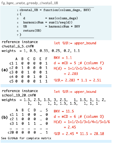
Figure 7: Two examples of computing the minimum set cover upper bound UB. The first instance is a test case introduced in [23].

The next section introduces a simplification of the greedy algorithm, replacing the isomorph-based solver unate_greedy_chvatal_iso with an alternative solver, unate_greedy_chvatal_stoc.

(a)

 

1unate_greedy_chvatal_basic = function()

2{

3  # required inputs

4  n           = glob[["nCols"]]

5  m           = glob[["mRows"]]

6  M           = glob[["M_ref"]]

7  colWeights  = glob[["colWeights_ref"]]

8  # local initializations

9  nOps        = 0

10  coord       = rep(0, n)

11

12  while(TRUE) {

13    percentages = colWeights / colSums(M)

14    if (all(percentages == Inf)) { break }

15    jdx         = which.min(percentages)

16    rem_vec     = which(M[,jdx] %in% 1)

17    M[rem_vec,] = 0

18    coord[jdx]  = 1

19    nOps        = nOps + 1

20  }

21  coordGreedy = paste(coord, collapse = "")

22  valueGreedy = as.numeric(t(coord) %*% colWeights))

23

24  return(list(

25    coordGreedy = coordGreedy,

26    valueGreedy = valueGreedy,

27    nOps        = nOps))

28}

 

 

1unate_greedy_chvatal_iso = function(replicaId=0)

2{

3  # required inputs

4  n               = glob[["nCols"]]

5  m               = glob[["mRows"]]

6  M_ref           = glob[["M_ref"]]

7  colWeights_ref  = glob[["colWeights_ref"]]

8  greedyId        = glob[["greedyId"]]

9  if (replicaId == 0) {

10    coordPermV = 1:n # reference permutation (natural order)

11    coordPerm  = paste(coordPermV, collapse=",")

12    colWeights = glob[["colWeights_ref"]]

13    M          = glob[["M_ref"]]

14

15  } else {

16    # create an isomorph instance, controlled by replicaId

17    set.seed(replicaId)

18    coordPermV = sample(1:n)

19    coordPerm  = paste(coordPermV, collapse=",")

20    colWeights = c()

21    M          = matrix(rep(NA, m*n), ncol=n)

22    for (idx in 1:n) {

23      i = idx

24      j = coordPermV[idx]

25      colWeights[idx] = glob[["colWeights_ref"]][j]

26      M[ ,idx]        = glob[["M_ref"]][,j]

27    }

28  }

29  # invoke unate_greedy_chvatal_basic() with new variables

30  glob[["M_ref"]]          = M

31  glob[["colWeights_ref"]] = colWeights

32  glob[["replicaId"]]      = replicaId

33  answ = unate_greedy_chvatal_basic()

34

35  coordGreedy = answ$coordGreedy

36  valueGreedy = answ$valueGreedy ; nOps = answ$nOps

37  return(list(coordGreedy=coordGreedy,

38              valueGreedy=valueGreedy, nOps=nOps))

39 }

 

(b)

 

1unate_greedy_chvatal_stoc = function()

2{

3  # required inputs

4  M          = glob[["M_ref"]]

5  n          = glob[["nCols"]]

6  m          = glob[["mRows"]]

7  colWeights = glob[["colWeights_ref"]]

8  replicaId  = glob[["replicaId"]]

9  # local initializations

10  nOps       = 0

11  coord      = rep(0, n)

12

13  while(TRUE) {

14    percentages = colWeights / colSums(M)

15    if (all(percentages==Inf)) { break }

16    if (replicaId == 0) {

17      jdx     = which.min(percentages)

18    } else {

19      jdx_vec = which(percentages == min(percentages))

20      jdx_cnt = sample(1:length(jdx_vec))[1]

21      jdx     = jdx_vec[jdx_cnt]

22    }

23    rem_vec     = which(M[,jdx] %in% 1)

24    M[rem_vec,] = 0

25    coord[jdx]  = 1

26    nOps        = nOps + 1

27  }

28

29  coordGreedy = paste(coord, collapse = "")

30  valueGreedy = as.numeric(t(coord) %*% colWeights))

31

32  return(list(

33    coordGreedy = coordGreedy,

34    valueGreedy = valueGreedy,

35    nOps        = nOps))

36}

 

 

1unate_greedy_chvatal_stoc_experiments =

2  function(instanceDef, isSeedConsecutive=T, replicateSize=10) {

3

4  # read instance file and convert to matrix with detailed info

5  # data store in global list, glob

6

7  read_bgu(instanceDef)

8  dt = data.table()

9  for (replicaId in 0:replicateSize) {

10

11    glob[["replicaId"]] = replicaId

12    if (isSeedConsecutive) {

13      seedInit = replicaId

14    } else {

15      seedInit = trunc(1e6*runif(1))

16    }

17    set.seed(seedInit)

18

19    answ = unate_greedy_chvatal_stoc()

20    coordGreedy = answ$coordGreedy

21    valueGreedy = answ$valueGreedy ; nOps = answ$nOps

22    dt = rbind(dt, list(

23      replicaId   = replicaId,

24      nOps        = nOps,

25      coordGreedy = coordGreedy,

26      valueGreedy = valueGreedy

27    ))

28  }

29  return(dt)

30

31}

 

Figure 8: Two equivalent stochastic versions in R of the Chvatal’s algorithm: (a) inducing distributions of set covers with bigraph isomorphs and (b) inducing distributions of set covers by randomizing best selections. To achieve the randomization, when ${\rm replicaId}>0$, we use the random selection returned by the R-function ”which”.

4.2 On Set Covers with a Stochastic Greedy Algorithm

The simplified stochastic greedy algorithm, replacing the isomorph-based implementation, is represented by the function unate_greedy_chvatal_stoc in Figure 8b. The distributions of set cover solutions are induced, for ${\rm replicaId}>0$, by relying on the randomized selections returned by the R-function ”which”.

How can we claim that the very different implementations of the two greedy stochastic algoritms in Figures 8a and 8b are equivalent? In Figures 8a we induce randomization by explicitly interchanging rows in the matrix. In Figures 8b we induce randomization by a random selection of columns with the same minimum rate between column weight and column degree.

Experiments have demonstrated, for both solvers, the same or close to the same distributions of ratios such as shown in Table 2, and Figure 9. However, the runtime of unate_greedy_chvatal_stoc solver that relies on changing the seed has better runtime and easier interpretation than unate_greedy_chvatal_iso solver that relies on explicit permutations of matrix columns. For specific isomorphs of interest, we do invoke a column permutation of the respective reference instance such as the example of instance school_5_5_ref.

4.3 Runtime Experiments

The runtime experiments with the minimum set cover instances are summarized in Figure 9, Table 1, Table 3, and Table 4.

(school_9_11.cnfU)
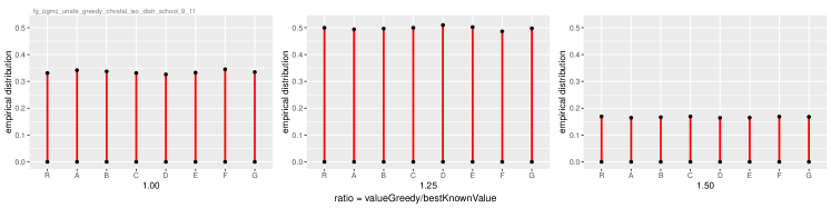
(ab)

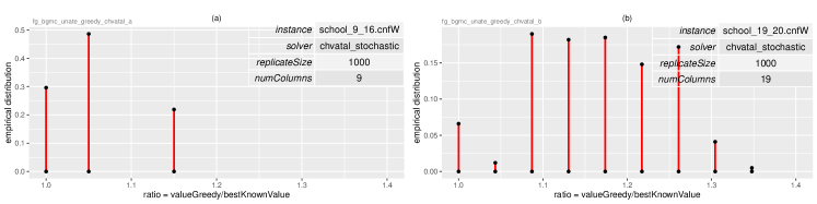
(cd)

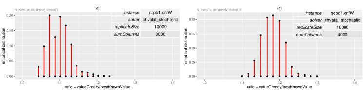
Figure 9: Reference parameters for each instance in this figure are listed in Table 1. The top segment (school_9_11.cnfU) depicts the empirical distribution of ratios {1.0, 1.25, 1.5} for the 8 isomorph classes of size 10,000 each, induced by the instance school_9_11.cnfU. The middle segment (ab) depicts distribution of ratios for two isomorph classes, each of size 1,000. The bottom segment (cd) depicts distribution of ratios the for two isomorph classes, each of size 10,000. For additional details, see the article.

Figure 9

The top segment (school_9_11.cnfU) depicts the empirical distribution of ratios {1.0, 1.25, 1.5} for the 8 isomorph classes of the instance school_9_11.cnfU. This instance, already introduced in Figure 4, induces isomorph classes {R, A, B, C, D, E, D,F, G}. The reference class R represents 10,000 instance isomorphs of school_9_11_R = school_9_11. The alternative class A represents 10,000 instance isomorphs of school_9_11_A = (seed-specific isomorph of school_9_11). The remainder of classes, {B,…,G}, are formed similarly. The empirical distribution probabilities associated with each ratio of the reference isomorph class R of size 10,000 are itemized below:

 

1   ratio ratio_cnt empirical_distr

21:  1.00      3311          0.3311

32:  1.25      4998          0.4998

43:  1.50      1691          0.1691

 

As shown in the plot, empirical distributions of ratios of the isomorph in classes from {A,…,G} closely match the reference isomorph class R. However, the variance between the isomorph classes becomes noticeable with decreasing the class size from 10,000 to 1,000 and 100 – just as already observed in Table 2.

The middle segment labeled as (ab) depicts distribution of ratios for two isomorph classes, each of size 1,000: weight-specific school_9_16.cnfW and weight-specific school_19_20.cnfW. For the school_9_16.cnfW isomorph class, we observe 3 distinct ratios in the range {1.0, 1.15}. For the school_19_20.cnfW isomorph class, we observe 9 distinct ratios in the range {1.0, 1.35}.

The bottom segment of this figure, labeled as (cd) depicts the empirical distribution of ratios for two isomorph classes, each of size 10,000: weight-specific scpb1.cnfW and weight-specific scpd1.cnfW. For the scpb1.cnfW isomorph class, we observe 14 distinct ratios in the range {1.04, 1.23}. For the scpd1.cnfW isomorph class, we observe 13 distinct ratios in the range {1.10, 1.30}.

Table 1

This table introduces all instances that summarize results of experiments in this article. Details about instance parameters have been discussed in Section 3 when introducing the maximum matching solvers. Additional columns in this table, relevant to the minimum set cover solvers in this section include BKV, UB, value_Chvatal_stats, and BKV_ratio_stats. The definition of ratio in Equation 1 relies on the best-known-value BKV. The computation of the Chvatal’s upper bound UB on the minimum set cover is illustrated in Figure 7. The column value_Chvatal_stats reports the empirical set cover statistics with solver unate_greedy_chvatal_stoc, the stochastic version of the Chvatal’s greedy algorithm. The reported statistics represents comma-separated values of minimum, median, mean, standard deviation, and maximum. The column BKV_ratio_stats reports the same statistics, normalized with respect to BKV.

There are 37 instances in Table 1. The question arises of how effective the stochastic greedy algorithm solver unate_greedy_chvatal_stoc actually is. A partial glimpse is shown in the table below:

 

1    ranges_of_ratios  counts_out_of_37

2        ratio  = 1.0                12

31.00 <  ratio <= 1.1                18

41.20 <= ratio <= 2.5                 7

 

The counts about in the table above signify:

• optimum solutions have been found for 12-out-37 instances,

• solutions within 10% of the optimium have been found for 18-out-37 instances,

• solutions above 20% of the optimium have been found for 7-out-37 instances.

Table 3: Similar size instances and their variabilities: BKVs, UBs, Chvatal ratios, and harmonic numbers. For details, see the article.

 

1                                    exact                                chvatal  chvatal

2                                    column_solutions/                    best     worst   harmonic

3instance             weight_range   column_degrees        BKV      UB    ratio    ratio     number

4school_19_20.cnfU    [1.0,   1.0]   2,4,5,6,15,16/         6      14.7    1.0      1.0      2.45

5                                    5,6,5,1, 3, 3

6school_19_20.cnfW    [1.0,   3.0]   1,5,7,9,10,14,17,18/  11.5    28.18   1.0      1.348    2.45

7                                    3,5,3,2, 4, 2, 2, 2

8school_19_20_1.cnfW  [0.333, 1.0]   1,5,7,9,10,14,17,18/   3.833   9.39   1.087    1.304    2.45

9                                    3,5,3,2, 4, 2, 2, 2

10school_19_20_5.cnfW  [0.7,   4.9]   1,4,5,7,9,15,16/      16.1    39.45   1.087    1.087    2.45

11                                    3,6,5,3,2  3, 3

12chvatal_19_18.cnfW   [0.33,  1.1]   19/                    0.5     1.75   1.0      1.0      3.496

13                                    18

 

Table 3

This table assembles four versions of 19-column, 20-row instance school_19_20: one with all weights at 1, and three with weights in the ranges shown. The fifth instance, chvatal_19_18, is a scaled-up instance of chvatal_6_5 introduced in [23]. In chvatal_6_5, only the weight of the column 6 determines its BKV. In chvatal_19_18, BKV = 0.5 for the solution column 19 and weight = 0.5. For more observations, see below:

• As already demonstrated in Table 1, the ratios UB/BKV $>$ 2, i.e. UB is not a tight upper bound. Weight range impacts UB significantly.

• Weight range also impacts significantly the minimum and the maximum range of ratio returned by the solver unate_greedy_chvatal_stoc. The harmonic number is determined by max(column_degrees) only. The ratio harmonic_number/worst_ratio) varies from 2.35/1.348 = 1.743 to 3.496.

Table 4: This is an extension of Table 1. The rows 3–5 refer to three large instances from the OR-library [18]. The rows 6–8 introduce almost identical instances related to instances on rows rows 3–5 with the exception that now all weights are set to 1. For details, see the article.

 

1                     chvatal         BRKGA      chvatal  chvatal     BRKGA    BRKGA

2  instance   BKV  cover_best    cover_best    num_seeds  seconds  num_gens  seconds

3scpb1.cnfW    69          72            69       10,000    1,271       200    2,505

4scpc1.cnfW   227         249           227       10,000    2,601       200    5,274

5scpd1.cnfW    60          66            60       10,000    1,666       200    5,377

6scpb1.cnfU    22          22            25       10,000      838       200    3,078

7scpc1.cnfU    44          44            47       10,000    1,444       200    4,764

8scpd1.cnfU    25          25            27       10,000    1,120       200    5,713

 

Table 4

This table supplements the results of the greedy set cover experiments summarized in Table 1. The six instances from Table 1 summarize the most important results obtained to date with the solver unate_greedy_chvatal_stoc, running each instance with 10,000 unique seeds, equivalent to processing 10,000 isomorphs of each of six instances.

• The rows 3–5 refer to three large instances from the OR-library [18]. Experiments with these instances verify the nominal performance of the C++ solver BRKGA [35, 36] reporting the minimum cover value found after running each instance with the generation limit of 200. The best covers returned by this solver match the BKVs reported elsewhere [37]: {69, 227, 60}. These covers dominate the best covers returned by unate_greedy_chvatal_stoc: {72, 249, 66}.

• The rows 6–8 introduce almost identical instances related to instances on rows rows 3–5 with the exception that now all weights are set to 1. There are no better covers than the ones reported by R solver unate_greedy_chvatal_stoc in this article: {22, 44, 25}. The best covers returned by C++ solver BRKGA are significantly worse: {25, 47, 27}.

The results on lines 6–8 in Table 4 are new: they provide the currently best-known-values (BKVs) for the three largest OR-instances listed on lines 6–8. This may well be the first time where a greedy algorithm outperforms a state-of-the-art algorithm designed to search for optimum solutions – not only in runtime but more importantly, in delivering significantly better solutions.

5 Summary and Future Work

The roots for this article have been provided by the rather unexpected empirical result in December 2020, as a follow-up on the just completed CSC316 Java project in a junior-level course in data structures and algorithms [5]. This result is summarized with two asymptotic plots, Figure 2a and Figure 2b. Elements of surprise include not only the significant runtime improvements with R-code versus the Java-code but also that these results were produced in a time frame of two weeks by the first author who was completely new to R. However, as it frequently happens, the time required to explain a new result can be much longer than the time required to produce the result itself.

Note

For all datasets, programs and asymptotic experiments with data structures in this article, see [22].

Summary

• Our model of movieLib in Figure 1b is a simplified case of an affiliation bipartite graph. For example, the first sentence from [38] begins with ‘Many real-world large datasets correspond to bipartite graph data settings—think for example of users rating movies or people visiting locations’.
  Data structures in R may well provide an advantage over Java for the class of affiliation bipartite graphs.

• The maximum bipartite matching experiments in Figure 5 consistently demonstrate the runtime advantages of R data structures in comparison with Java.

• The introduction of two stochastic algorithms demonstrates advantages of greedy heuristic for the set cover problem. The merits of rapid prototyping these algorithms in R is apparent by the simplicity and the readability of the code in Figure 8.

• The results on lines 6–8 in Table 4 provide the currently best-known-values (BKVs) for the three largest OR-instances listed on lines 6–8. By significantly outperforming a state-of-the-art algorithm designed to search for optimum solutions – not only in runtime but more importantly, in delivering significantly better solutions – these greedy solutions provide a strong basis and motivation for future work.

Future Work

• The current work focuses on completing two companion articles, [2] and [3]. Both provide support and components for for the work in this article as well as for the articles to follow.

• In the immediate future, methods that produced the results on lines 6–8 in Table 4 of this paper will provide the basis for new methods in stochastic combinatorial optimization.

References

- [1] Z. Füredi, Matchings and Covers in Hypergraphs, Graphs and Combinatorics 4 (1988) 115–206.
- [2] F. Brglez, E. Li, Empirical Models of Key/Coupon Problems: from Urns and Dice to Layered Sparse Regular Graphs, Work in progress. A preprint available on request. (2022).
- [3] F. Brglez, E. Li, Multiwalk Stochastic Solver Alternatives for Set Cover Minimization: Principles and Components, Work in progress. A preprint available on request. (2022).
-
[4]
R Core Team, R: A Language and Environment
for Statistical Computing, R Foundation for Statistical Computing,
Vienna, Austria (2021).
URL https://www.R-project.org/ - [5] CSC316: Data Structures and Algorithms , https://www.engineeringonline.ncsu.edu/course/csc-316-data-structures-and-algorithms/ (2020).
- [6] IMDb Datasets, https://www.imdb.com/interfaces/ (2021).
- [7] N. L. Johnson, S. Kotz, Urn models and their applications: an approach to modern discrete probability theory, Wiley, 1977.
- [8] Guava: Google Core Libraries for Java, https://github.com/google/guava (2021).
- [9] Homepage of net.datastructures at the the Brown University, http://cs.brown.edu/cgc/net.datastructures.net/ (2014).
- [10] R Data Frames, http://www.r-tutor.com/r-introduction/data-frame (2021).
- [11] R Data Tables, htps://cran.r-project.org/web/packages/data.table/vignettes/datatable-intro.html (2021).
- [12] T. H. Cormen, C. H. Leiserson, R. L. Rivest, Introduction to Algorithms, McGraw-Hill Book Company, 1990.
- [13] L. R. Ford, D. R. Fulkerson, Maximal Flow through a Network, Canad. J. Math 8 (1956) 399–404.
- [14] J, E. Hopcroft and R. M. Karp, An Algorithm for Maximum Matchings in Bipartite Graphs, SIAM Journal on Computing 2 (4) (1973) 225–231.
- [15] Maximum Bipartite Matching: Java Code , https://www.geeksforgeeks.org/maximum-bipartite-matching/ (2021).
- [16] G. Csárdi and T. Nepusz, Maximum Bipartite Matching: R Code, https://igraph.org/r/doc/matching.html (2021).
-
[17]
M. G. C. Resende, Steiner
Triple Covering Problems (2021).
URL http://mauricio.resende.info/data/index.html - [18] J. E. Beasley, OR-Library, http://people.brunel.ac.uk/~mastjjb/jeb/orlib/scpinfo.html (2021).
- [19] Logic Synthesis Workshops 1989, 1991, 1993, The Benchmark Archives at CBL (up to 1996, https://people.engr.ncsu.edu/brglez/CBL/benchmarks/Benchmarks-upto-1996.html (1993).
- [20] Conjunctive normal form, https://en.wikipedia.org/wiki/Conjunctive_normal_form (2021).
- [21] X. Y. Li, M. F. Stallmann, F. Brglez, Effective bounding techniques for solving unate and binate covering problems, in: DAC ’05: Proceedings of the 42nd annual conference on Design automation, ACM, New York, NY, USA, 2005, pp. 385–390, http://doi.acm.org/10.1145/1065579.1065682.
- [22] E. Li, F. Brglez, Datasets, Programs and Asymptotic Experiments with Data Structures: Bipartite Graph Matchings and Covers, https://github.com/rBedPlus/rBed_bgmc (2021).
- [23] V. Chvatal, A Greedy Heuristic for the Set-covering Problem, Mathematics of Operations Research 4 (3) (1979) 233–235.
- [24] N. E. Young, Greedy Set-Cover Algorithms (Part 7 of Encyclopedia of Algorithms), Springer Encyclopedia of Algorithms (2016) 886–889.
- [25] H. A. Simon, J. R. Hayes, The understanding process: problem isomorphs, Cognitive Psychology 8 (1976) 165–190, reprinted in MOT1, Chap. 7.2.
- [26] G. Gunzelmann, J. R. Anderson, An ACT-R model of the evolution of strategy use and problem difficulty, in: Proceedings of the Fourth International Conference on Cognitive Modeling, 2001, pp. 109–114, mahwah, NJ: Lawrence Erlbaum Associates.
- [27] H. A. Simon, Models of my life, MIT Press, 1996.
- [28] J E. Harlow III and F. Brglez, Design of Experiments and Evaluation of BDD Ordering Heuristics, International Journal on Software Tools for Technology Transfer (STTT) 3 (2) (2001) 193–206, http://www.springerlink.com/content/15en21tldhrw08nt/.
- [29] M. Stallmann, F. Brglez, D. Ghosh, Heuristics, experimental subjects, and treatment evaluation in bigraph crossing minimization, J. Exp. Algorithmics 6 (2001) 8, http://doi.acm.org/10.1145/945394.945402. doi:http://doi.acm.org/10.1145/945394.945402.
- [30] F. Brglez, X. Y. Li, M. F. Stallmann, On SAT instance classes and a method for reliable performance experiments with SAT solvers., Ann. Math. Art. Intell. 43 (1) (2005) 1–34.
-
[31]
Performance Testing of
Combinatorial Solvers With Isomorph Class Instances.
URL http://doi.acm.org/10.1145/1281700.1281713 -
[32]
R. Saket and M. Sviridenko,
New and Improved Bounds
for the Minimum Set Cover Problem, Lecture Notes in Computer Science,
APPROX 2012, RANDOM 2012 (2012).
URL https://doi.org/10.1007/978-3-642-32512-0_25 - [33] G. Felici, S. Ndreca, A. Procacci, B. Scoppola, A-priori upper bounds for the set covering problem, Annals of Operations Research 238 (2016) 229–241.
-
[34]
A. Abboud, R. Addanki, F. Grandoni, D. Panigrahi, B. Saha,
Dynamic set cover: Improved
algorithms and lower bounds, in: Proceedings of the 51st Annual ACM SIGACT
Symposium on Theory of Computing, STOC 2019, Association for Computing
Machinery, 2019, pp. 114–125.
URL https://doi.org/10.1145/3313276.3316376 -
[35]
R. Toso, M. Resende, A C++
application programming interface for biased random key genetic algorithms,
Optimization Methods and Software (2014).
URL doi:10.1080/10556788.2014.890197 - [36] J. F. Gonçalves, M. G. Resende, R. F. Toso, An Experimental Comparison of Biased and Unbiased Random-Key Genetic Algorithms, Pesq. Oper. 34 (2), https://www.scielo.br/j/pope/a/wZhhVnhhPkGkKCHttwfTgwd/?lang=en (5-8 2014).
- [37] B. Crawford, R. Soto, R. Cuesta, F. Paredes, Application of the Artificial Bee Colony Algorithm for Solving the Set Covering Problem, The Scientific World JournalSwarm Intelligence and Its Applications 2014, https://doi.org/10.1155/2014/189164 (2014).
-
[38]
M. Stankova, S. Praet, D. Martens, F. Provost,
Node classification over
bipartite graphs through projection, Machine Learning 110 (1) (2021) 37–87.
URL https://doi.org/10.1007/s10994-020-05898-0