Correlation inequalities for the uniform 8-vertex model and the toric code model
Abstract.
We elucidate connections between four models in statistical physics and probability theory: (1) the toric code model of Kitaev, (2) the uniform eight-vertex model, (3) random walk on a hypercube, and (4) a classical Ising model with four-body interaction. As a consequence of our analysis (and of the GKS-inequalities for the Ising model) we obtain correlation inequalities for the toric code model and the uniform eight-vertex model.
1. Introduction
Recent years has seen a rapid development of research on vertex models, primarily the six-vertex model. The six-vertex model was originally introduced by Pauling as a simple model of hydrogen bonding in water ice. Lieb [17, 18, 19] carried out pioneering work on the model using the Bethe Ansatz originally developed for the Heisenberg spin chain. Recently, the model has received growing attention from the probability community, with several rigorous results as a consequence, e.g. [7, 8, 12].
The eight-vertex model is a generalisation of the six-vertex model that allows two extra types of vertices: sources and sinks. Both the six- and eight-vertex models are integrable lattice models [11, 23]. Using methods coming from integrability, Baxter [4] computed the free energy per site. For information on integrable models we direct the reader to the book by Baxter [5].
In this work we consider the eight-vertex model from a different perspective than solvability/integrability. We consider some simple dynamics which preserve eight-vertex configurations: select a plaquette (face) of the square lattice at random and reverse the direction of its four bounding edges. Because every vertex has an even number (either zero or two) of its incident edges reversed, these dynamics preserve the set of allowed configurations. (A variant of the dynamics preserves the six-vertex model and is in fact in detailed balance with the six-vertex model’s probability distribution [1].)
There is a close connection between these dynamics and Kitaev’s toric code model. Kitaev’s model (at zero temperature) is an important example of a quantum code, which are motivated by problems in quantum computing. While quantum computers would allow certain computations to be performed much faster than a conventional computer (e.g. factoring large numbers [21] or searching unstructured databases [13, 14]), a major barrier in realising this potential is the proclivity for the quantum bits (qubits) of the computer to to have errors. One way to try to overcome this problem is to use multiple physical qubits to encode a single logical qubit that performs better than its individual physical qubit components, primarily due to the ability to recover the intended state of the logical qubit even after one or more of the component physical qubits has experienced an error. We direct the reader to [20] for an accessible treatment of major topics in quantum information and quantum computation. Surface codes, of which Kitaev’s toric code is an example, are examples of such a scheme that have enjoyed huge amounts of attention, in part due to their relatively high tolerance for local errors [22]. For an introduction to the various aspects of the toric/surface code and how it operates we direct the reader to the review [10].
Using the dynamics indicated above facilitates explicit computations of certain thermodynamic quantities for the toric code model at positive temperature. Guided by these calculations and their consequences, we establish a connection between certain correlations in the toric code model and expectations in a many-body classical Ising model. The ground state of the latter Ising model also gives the eight-vertex model with uniform vertex weights. Using well-known correlation inequalities for the Ising model (GKS) we obtain correlation inequalities for the uniform eight-vertex model and the toric code model. The following is an example of our correlation inequality for the uniform eight-vertex model: given any two sets of vertices, consider the events that they are all sources or sinks. Then these events are positively correlated, i.e. the probability of both occurring is at least as large as the product of the probabilities of the two individual events. The full statement appears in Theorem 1.1.
1.1. Setting and results
For , let . We view as the vertex set of the torus . (It is possible to work with as a subset of with a boundary; we do this in Section 4.) Let denote the set of edges of and the set of faces. In keeping with common terminology in the area, faces will often be referred to as plaquettes and denoted , and vertices referred to as stars and denoted .
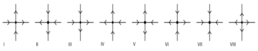
The first model we consider is the uniform eight-vertex model, defined as follows. Let denote the set of assignments of directions to the edges , meaning that each horizontal edge is directed either or , and each vertical edge either or . Elements of will sometimes be referred to as arrow-configurations. Let denote the set of arrow-configurations such that the number of arrows pointing towards any vertex is even. At each vertex , there are eight possible configurations of arrows, depicted in Figure 1. We refer to these eight local configurations by the roman numerals . The first six of these are the allowed configurations for the six-vertex model; VII is called a sink and VIII a source. We let denote the uniform probability measure on ; this is the probability measure governing the uniform 8-vertex model.
The next model we consider is Kitaev’s toric code model [15], defined as follows. For the edge-set of the torus as above, let be the tensor product of one copy of for each edge . Using the standard basis , for , one obtains a (product) basis for with elements for . Consider the Pauli matrices
| (1) |
and write for the linear operator on which acts as on the factor and the identity elsewhere. Since each acts diagonally on the basis elements , we refer to this basis as the product basis.
Introduce the operators
| (2) |
where and mean that the edge is adjacent to the vertex or the face , respectively. (The operators and are more commonly denoted and , respectively.) For and vectors of constants satisfying , the Hamiltonian operator is defined as
| (3) |
For all this is Kitaev’s , see [15]. All terms in commute, since for any star and plaquette the number of edges belonging to both of them is even.
The Hamiltonian (3) governs the toric code model, for instance through the equilibrium states defined as follows: for an operator on ,
| (4) |
If we take we obtain the ground state which is important in the theory of quantum codes; see Appendix A. We will see below that the limit of all , with all fixed, essentially gives the uniform 8-vertex model.
By further relating the uniform 8-vertex model and the toric code model to a certain classical Ising model, defined in the next subsection, we will prove certain correlation inequalities. The setting is as follows. First, for the 8-vertex model, let be any 8-vertex configuration. Let be the event that, for each , the arrows around are either all equal to those of or all the opposite to those of . Additionally, for with let be the event that, for each , the arrows around are either all equal to those of or or all the opposite to those of or (this trivially includes the even when has all arrows opposite to those of ). For the toric code the setting is similar but more complex to state. For , consider the four edges , , and adjacent to and write for . Let , satisfying , be a local sign-configuration. Define the operators
| (5) |
and for let
| (6) |
For with define
| (7) |
Finally, we say that is contractible if does not contain a set of nearest-neighbour vertices that forms a non-contractible loop on the torus .
Theorem 1.1.
Let , , with and , be as above and let be sets of vertices such that
-
•
either is contractible,
-
•
or any non-contractible loop in has even length.
Then
-
(1)
For the uniform 8-vertex model: and
-
(2)
For the toric code model: and
As an example of the correlation inequality for the 8-vertex model, we can take to be the constant vector of all VII’s, i.e. only sinks. Then is the event that every vertex in is either a source or a sink, and the Theorem says that and are positively correlated. This is primarily interesting when and are not too far apart: we will see in Section 4.1 that if and are not adjacent to any common faces, then the states of the vertices in and are in fact independent under .
1.2. Relations between the models
As mentioned above, Theorem 1.1 builds on relating the two models (uniform 8-vertex and toric code) to a classical Ising model. We now define the latter. Let be a vector with all . Recalling that , define the probability measure on by
| (8) |
This is a ferromagnetic Ising model with four-body interaction, and the restriction of the toric code model to a certain class of observables is equivalent to this model:
Proposition 1.2.
Let be any observable diagonal in the product basis, say for any . Then
| (9) |
where denotes expectation with respect to . In particular, does not depend on .
Note also that if for all then is supported on the set of configurations satisfying for all , since attains its maximum value for such . This observation will allow us to (essentially) identify the uniform 8-vertex measure with .
The key fact we use about the Ising model (8) is that it satisfies GKS-inequalities (see e.g. [9, Theorem 3.49]): for any sets we have
| (10) |
The fourth model which we use in our analysis is simple random walk on the hypercube. To define this, let denote the two-element group with elements satisfying , and consider with generators given by
| (11) |
Then is a hypercube of dimension . A random walk on is given by selecting, independently at random, faces and letting where is a starting position. Here at each step we choose face with probability .
The relation to the previous models comes by letting act on the sets and . The intuition is simple: acts on elements of by reversing all the arrows around the face , and on by negating the signs on the edges surrounding . It is easy to see that this action leaves invariant, and also leaves the measures and invariant. The connection to the toric code model is slightly more subtle: we will see in Section 2.1 that the term in the Hamiltonian (3) is essentially the generator matrix of (the continuous-time version of) simple random walk on . This allows us to express the equilibrium states (4) for using transition probabilities for the random walk, which will be instrumental in understanding some basic features of the toric code model, including the relation to the Ising model, Proposition 1.2.
1.3. Acknowledgements
JEB gratefully acknowledges financial support from Vetenskapsrådet, grant 2019-04185, from Ruth och Nils Erik Stenbäcks stiftelse, and from the Sabbatical Program at the Faculty of Science, University of Gothenburg, as well as kind hospitality at the University of Warwick and the University of Bristol.
2. Properties of the toric code model
2.1. Dynamic description
Recall that (below (11)) we defined random walk on the hypercube as the process obtained by sampling independently at random faces and successively adding them to an initial element of . We make this into a continuous-time random walk using a Poisson process of rate and defining
| (12) |
An equivalent description is that each face is assigned an independent exponentially distributed random ‘clock’ of rate and that we add 1 in the postion of when the corresponding clock rings.
We next map the random walk (12) onto a process in as well as onto a process in the set of arrow-configurations. As already described for the discrete-time case, the process in proceeds by ‘flipping’ (negating) all signs on the edges around the selected face , and the process in similarly reverses the arrows around . We may describe this more formally as follows. The group acts on the set by
| (13) |
and denotes component-wise multiplication. (We are implicitly presenting as the multiplicative group with elements .) Then we define as the result of applying (13) for the randomly selected faces in (12):
| (14) |
Here is an initial configuration, and since the group is commutative we do not need to specify an order of multiplication in (14).
It will be useful to record here the generator-matrix for the random walk (14). Indeed, regarding the of (13) as a matrix with rows and columns indexed by , the generator matrix can be written as
| (15) |
where denotes the identity matrix. It follows that the transition-probabilities at time are given by the matrix
| (16) |
To formally define the process in , we note that we may think of as encoding an arrow-configuration in by indicating which edges are reversed (or not) with respect to some a-priori configuration of arrows. More precisely, fix a reference-configuration and define, for , the arrow-configuration such that the arrow at has the same orientation as in if , respectively the opposite orientation if . We then obtain a random walk by
| (17) |
Note that depends both on the reference-configuration and the initial sign-configuration .
We next describe the relevance of the random walk for the toric code model. Recall that the elements are in one-to-one correspondence with basis-vectors for , given as the product-basis obtained from the basis , for . Thus the action of on carries over to a representation of on . Moreover, from the explicit form of the Pauli-matrices (1) we see that . Thus the operator in (2) acts precisely as in (13). It follows from (15) that the term in the Hamiltonian (3) is, up to adding a multiple of the identity, the generator for a random walk on the set of basis-vectors.
We note here that the random walk on is not irreducible, i.e. the set decomposes into several disjoint communicating classes. See Proposition 4.1.
2.2. Duality
There are two useful notions of duality for the toric code model: that of the lattice as a planar graph, as well as a duality between the operators and . In this subsection we aim to make precise these dualities as well as the connection between them.
We start by looking at the operators and . Recall that we have been using a basis for in which is diagonal and the other Pauli matrices are given as in (1). For the rest of this subsection, we denote this basis by , where the subscript z serves to indicate that the third Pauli matrix is diagonal. The corresponding product basis for will be denoted for . Recall that, in this basis, the operator negates the signs on all edges surrounding , while is diagonal.
We can also consider a basis for in which is diagonal: define
| (18) |
The corresponding product basis for will be denoted for . The basis-change matrix for going between and is the symmetric, orthogonal matrix (the Hadamard matrix)
| (19) |
To go between the bases for one uses the -fold tensor product . This change of basis maps to and to , meaning that in the -basis, negates all the signs on the edges adjacent , while is diagonal.
What we have described so far dovetails with the planar duality of , as follows. Define the dual to be the graph with vertex set , edge-set , and faces . One obtains by placing a vertex in the middle of each face of and drawing edges perpendicularly across those of . In this way, any vertex of the orignal lattice lies in the middle of a unique face of the dual . We can then write, for and ,
| (20) |
As noted above, the operators and act on the -basis in the exact same way as and act on the -basis . Namely, is diagonal while negates the signs around . In this sense, going between the lattice and its dual is equivalent to changing basis between and . Some particular instances of this are the identities:
| (21) |
and for any , with corresponding dual sets , ,
| (22) |
These identities may all be obtained by conjugating with .
2.3. Consequences
We now provide some applications of the random-walk dynamics and of the duality. Write for the probability measure governing the process of (14) started at . We revert to the notation without a subscript for the usual basis defined above (1) and referred to as above.
Lemma 2.1.
For any and , we have the following matrix entries:
| (23) |
Moreover,
| (24) |
In particular, is constant on the diagonal.
Proof.
The first identity in (LABEL:eq:mtrx-entries) follows from the discussion at the end of Section 2.1, since is the matrix of transition-probabilities of . The second identity in (LABEL:eq:mtrx-entries) follows from the fact that is diagonal in the given basis, with entry precisely .
For (24), we see from (14) that if and only if either (i) each plaquette is flipped an even number of times, or (ii) each plaquette is flipped an odd number of times. The number of times a given plaquette is flipped by time is a Poisson random variable with parameter , and they are independent. This gives the stated expression. ∎
Lemma 2.1 allows for straightforward, explicit calculation of some thermodynamic quantities:
Proposition 2.2.
Proof.
For (25), note that
| (28) |
The first equality follows from the fact that the terms commute, the second equality from Lemma 2.1 and the elementary fact that if are matrices such that is diagonal and is constant on the diagonal. Next, from Lemma 2.1 we have
| (29) |
Also, from the duality-relations (21) we have
| (30) |
This follows by taking the trace in the -basis rather than the -basis.
For (26), we note that
| (31) |
where we used the fact that is diagonal. Next, using the notation of (13),
| (32) |
For the event in the probability to occur, either (i) all are flipped an odd number of times and all an even number of times, or (ii) vice versa. Computing this probability and using (30) and (25) gives (26). Finally, (27) follows from the duality (21). ∎
From (25) we immediately obtain an expression for the free energy of the system in the case when all and all :
| (33) |
In particular, is analytic for , indicating that the system does not undergo a phase transition, as pointed out earlier in e.g. [2].
Next we record a result complementary to Proposition 2.2 that will be useful in the proof of the correlation inequalities.
Proposition 2.3.
For define the operators
| (34) |
Then unless is a product of plaquette operators , i.e. unless for some . Similarly, unless is a product of star operators , i.e. unless for some .
Proof.
We prove the claim for ; the claim for follows by the duality (21). The expansion (31) remains valid with replaced by , and in place of (32) we find that
| (35) |
where is in position and elsewhere. Now if is not a product of plaquette operators then there is no realisation of the dynamics with the property that . Then , as claimed. ∎
We now turn to the Ising model (8) and Proposition 1.2. Recall that is assumed to be an operator on diagonal in the -basis with .
Proof of Proposition 1.2.
Remark 2.4.
-
(1)
Recall that the probability measure is invariant under reversing all the spin-values around any fixed plaquette . This immediately gives that if there is any plaquette such that contains an odd number of the edges surrounding , which is in line with Proposition 2.3.
- (2)
3. Correlation inequalities
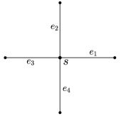
The proof of Theorem 1.1 will proceed by first proving a similar statement for the Ising model (8). To state the latter, we introduce the following notation. For consider the 4 edges , , and adjacent to , to be definite ordered as in Figure 2. For , write . We define the following quantities similar to (5) and (6): for satisfying , let
| (38) |
and for ,
| (39) |
Then is the indicator of the event that, for each , the values for either all agree with , or are all the opposite. Similarly to the eight-vertex model and toric code, for with we also define
| (40) |
Lemma 3.1.
Let , with , be as above and let be sets of vertices such that
-
•
either is contractible,
-
•
or any non-contractible loop in has even length.
Then for any such that all ,
| (41) |
and
| (42) |
The method of proof will be to expand the products defining and then apply the GKS-inequalities (10) to the terms of the expansion. The subtlety is that the terms come with signs; we show, using Proposition 2.3, that all terms with negative sign actually vanish in expectation.
Proof.
We will prove the first inequality, the proof of the second inequality is almost identical. Since , we have that where and (with the argument suppressed for readability)
| (43) |
Let be any of , or . By expanding the product over we get that
| (44) |
In this expression we expand the product over . To write the expansion, we use the following notation. We let denote the set of sequences of two-element subsets of , indexed by . We may represent such a subset pictorially as an element of the set , indicating the orientations of the two edges selected. Then,
| (45) |
Now consider an arbitrary term in the latter expansion, corresponding to a choice of , and sequence in . We write this term as
| (46) |
The following is the key claim: if can be written as a ‘product of stars’, then it comes with a positive sign. That is, if there is a set such that
| (47) |
then
| (48) |
Before proving the claim (i.e. that (47) implies (48)) we show how to deduce the result. We may write
| (49) |
where and are terms of the form (46) for and for , respectively, and is of the form (46) for . We will use the GKS-inequality (10) to see that all terms satisfy . By retracing the steps of the expansion, this implies the result. Now, if does not satsify (47) then at least one of and does not satisfy it either. By Propositions 1.2 and 2.3, then . If does satisfy (47) but one of and does not, then by Propositions 2.2 and 2.3, . Finally, if all three of satisfy (47) then the desired inequality follows from the GKS-inequality (10) and the fact that the terms have positive coefficients, thanks to the claim.
We now prove the claim that (47) implies (48). If (47) holds, then since the satisfy , we get
| (50) |
Recall that we represent each factor of the product over as an element of the set of shapes , indicating the two selected edges. Similarly, each factor of the product over may be represented as a , indicating that all four edges are selected. We think of the latter as consisting of two superimposed shapes, such as and (the precise choice does not matter).
We can assume that . Then we conclude from (50) that each edge appears in the product either exactly twice, or not at all. Consider now the subset of edges which appear exactly twice (counting each such edge once). Due to the possible choices of ‘shapes’ at each vertex, this subset forms an even subgraph (each vertex has even degree) and thus decomposes as a collection of closed loops. We claim that each such loop has the following property: the number of vertices where it exhibits a shape from is even, similarly the number of vertices where it exhibits a shape from is even, and finally the number of vertices where it exhibits a shape from is even. The latter claim can be seen by induction, as follows. We may take the loops to be non-crossing. For any non-crossing contractible loop enclosing at least two squares, we can decrease its enclosed area one square by removing a corner. As we do so, the number of shapes from each of the four sets changes by an even amount. Eventually the loop reduces to a single square, for which the claim holds by inspection. If the loop is not contractible, then a similar reduction can be used to reduce it to a ‘straight’ loop, which by our assumption on has even length, meaning again that the claim holds by inspection.
Proof of Theorem 1.1.
For the toric code model, note that the operators and are diagonal in the -basis and satisfy and . Then the result follows from Proposition 1.2 and Lemma 3.1.
For the uniform 8-vertex model we deduce the result by fixing a reference configuration and letting all . Since the limit of the Ising-measure (8) is uniform on , the distribution of is uniform on ∎
Remark 3.2.
It is possible, as in [3], to construct a quantum system generalising the Kitaev model, whose ground state configurations correspond to eight-vertex configurations with the general weights
| (52) |
depending on the numbers of vertices of the different types. However, the operators that must be added to the hamiltonian to achieve this do not satisfy the required non-negativity. This suggests that the inequalities in Theorem 1.1 may not hold for non-uniform weights.
Using almost the same argument as for Lemma 3.1 we can also prove the following:
Proposition 3.3.
For any and any satisfying , as above,
| (53) |
In particular, for any ,
| (54) |
Proof.
4. Further results for the uniform 8-vertex model
In this section we discuss some further properties of the uniform eight-vertex model that are natural to consider from the viewpoint of ‘plaquette-flipping’.
4.1. Communicating classes
We start by considering the communicating classes of the dynamics (17) in the case when all . Recall that is an torus.
Proposition 4.1.
We have that , and there are four communicating classes for the dynamics (17), each of size . We may move between them by reversing arrows along a non-contractible path in .
Proof.
We start by showing that . First, clearly . By fixing a reference-configuration as in (17) we can encode each element of using an element where is the two-element field. Then, for each , the constraint that has an even number of incoming arrows becomes a linear constraint over , namely where (similarly to (11))
| (57) |
and is the scalar product. These constraints are not linearly independent, since for each . However, this is the only linear relation: any other linear relation would have to be of the form for some proper subset of . But then there must be some edge with precisely one end point in and then . From this and the rank-nullity theorem we get that , as claimed.
Now it is simple to see that there are four communicating classes for the dynamics. There are plaquettes in and hence possible sums for . However, we have that (since ). Hence, starting from any reference configuration , there are configurations reachable by flipping plaquettes. This shows that there are four communicating classes.
Lastly, let be a non-contractible path of edges in , it is clear that such a path is not the boundary of a collection of plaquettes . This means that the configuration obtained by reversing arrows on is not reachable from the reference configuration via the dynamics. There are two homotopy classes of non-contractible paths on the torus and reversing arrows along a path of edges in one or two of the classes moves us between the four communicating classes. ∎
Remark 4.2.
-
(1)
Because our dynamics for the uniform eight-vertex model correspond to a random walk on the hypercube , we can import results about mixing times from the literature. For example, the mixing time for the dynamics is (recall that the Poisson process of steps has rate rather than the usual rate 1). The interested reader can consult [16] and references therein for detailed statements.
-
(2)
The limiting distribution of random walk on the hypercube is uniform. This leads to a method for sampling from the uniform eight-vertex distribution : first sample uniformly a representative from each of the four communicating classes to act as reference-configuration, then toss independent coins for each of the plaquettes for whether to ‘flip’ the plaquette or not.
-
(3)
If are vertices not adjacent to any common plaquette , then by the previous item, the vertex-types at and can be written as functions of independent random variables (states of the plaquettes surrounding them). Thus their states are independent.
4.2. Emptiness formation probability
In this subsection we allow to view not only as a torus, but also as a subset of with a boundary. In that case we replace each of the edges of the form with two boundary-edges and , and similarly replace each with two boundary-edges and .
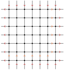
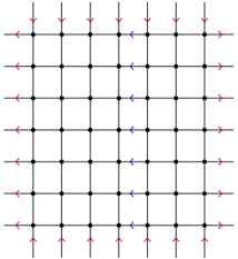
First we consider the domain wall boundary condition. This means that the top and bottom boundary edges (of the form or ) receive the fixed orientation pointing in towards , and that the left and right boundary-edges (of the form or ) are fixed to point out of . See Figure 3 for an illustration.
We emphasise and by using the notation . We denote by the set of eight-vertex configurations on with domain wall boundary conditions as described above.
Proposition 4.3.
Proof.
We begin by showing that if and only if is even. This is done in three steps.
Step 1: if then . Indeed, Figure 3 illustrates how an element of can be ‘extended’ to an element of .
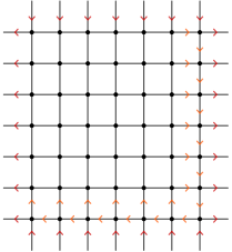
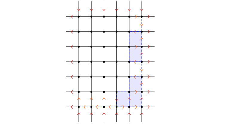
Step 2: conversely, if then . Indeed, fix an element and consider the bottom row of vertical edges and the rightmost column of horizontal edges in (see Figure 4). If all those vertical edges are oriented in, and all the horizontal ones are oriented out, then the restriction of to is an element of . Otherwise, the edges pointing the ‘wrong way’ (i.e. out for vertical edges on the bottom, in for horizontal edges on the right side) will be called faults. It is not hard to check that the number of faults must be even. Then, pair up the successive faults and mark the plaquettes between the pairs, as in Figure 4. Flipping all the marked plaquettes maps to a configuration whose restriction to is an element of .
Step 3: from the previous two steps we see that if and only if . If this holds if and only if ; if it holds if and only if . It is straightforward to check that the latter sets are non-empty if and only if is even, which is equivalent to being even.
To determine the number of configurations when is even, we use a simple counting argument. First, let us count the number of choices at each vertex if we start at the top left corner and proceed left to right and then top to bottom. As we proceed, each time we ‘arrive’ at a new vertex except the rightmost column or bottom row, exactly two incident arrows are already fixed, leaving us with exactly two choices. In the rightmost column and bottom row, three incident arrows are fixed when we arrive, leaving us at most one (possibly no) choice per vertex. This gives that
| (59) |
On the other hand, if , fix some . An argument similar to that of Proposition 4.1 shows that, in this case, the number of configurations reachable by flipping plaquettes equals the total number of configurations. Since there are plaquettes, this gives that
| (60) |
Combining (59) and (60) shows that, when non-empty, has size . The claim about irreducibility follows from the proof of (60). ∎
We now turn our attention to the so-called emptiness formation probability of the model. This is the probability that a fixed column of horizontal edges has all of its arrows pointing to the left (say). In this case we say that the column is empty. Denote by the event that the column of horizontal edges whose left end-points have first coordinate is empty, see Figure 5. In what follows, denotes the uniform probability measure on . We calculate the probability of in the case of the torus and the case of domain wall boundary conditions. We begin with the domain wall case.
Proposition 4.4.
Assume that is even so that . Then
Proof.
The proof is similar to that of Propositon 4.3. First we show that if and only if is even. Indeed, by Propositon 4.3, the part of to the right of the empty column can be ‘filled in’ if and only if is even. Since is even, this is equivalent to being even. To fill in the part to the left of the empty column, we can make the top row alternate between types VI and VII (also this is possible if and only if is even) and the rest all type IV. (Recall Figure 1 for the vertex types.) This shows that if and only if is even.
Assuming then that is even, let us count the number of choices at each vertex in the two parts, going from left to right and then top to bottom in each. We see that vertices have two choices of vertex type and the remaining vertices have at most one choice. From this and Proposition 4.3 we see that
| (61) |
On the other hand, consider the plaquettes that may be reversed without affecting the empty column. Similarly to the proof of Proposition 4.3 we see that each distinct choice gives a different configuration. From this we have that
| (62) |
which completes the proof. ∎
In the case when is viewed as a torus, the emptiness formation probability is independent of the position of the empty column. We hence simply denote by the event that an arbitrary, fixed, column of the torus is empty. Recall that is the uniform distribution on eight-vertex configurations.
Proposition 4.5.
Consider with sides identified to form a torus. Then
Proof.
Let us fix the column that is to be empty as the rightmost column. First, it is simple to see that as the configuration consisting of all vertices being type II has all columns empty. For an upper bound on we again use a simple counting argument. By fixing the vertex types starting from left to right and then top to bottom, we see that the leftmost column has one fixed incident arrow, hence these vertices have four choices. The ‘bulk’ vertices have two choices and the remaining vertices have at most one choice. We therefore have that
| (63) |
On the other hand, consider the plaquettes whose bounding arrows can be reversed without affecting the empty column. Note that distinct choices of which plaquettes to reverse give different configurations (we can now only reverse plaquettes in one of and not both because one of contains the plaquettes of the empty column). Thus we can obtain distinct configuration in from a fixed reference configuration. Next, note that if we reverse all arrows along a straight, vertical, non-contractible path of vertices away from the rightmost column, then we obtain a configuration in that can not be reached from the reference configuration by reversing arrows around plaquettes. By now reversing around plaquettes from this new eight-vertex configuration we find another distinct configuration with the empty column. This gives that
| (64) |
which matches our upper bound. ∎
4.3. Entropy
Now we consider the entropy of the model, meaning that we compare the number of eight-vertex configurations for various boundary conditions. We will suppose that are fixed such that is even and we revert to the notation without subindices. Let be a fixed assignment of arrows to the boundary edges (i.e. the edges , , and ) and denote by the set of eight-vertex configurations on with the boundary configuration . We call valid if .
Proposition 4.6.
A boundary condition is valid if and only if the number of arrows around the boundary of that point into is even. In this case .
Proof.
If , then the same argument as in the proof of Proposition 4.3 shows that all configurations in are reachable by flipping plaquettes, and thus . It remains to determine when .
Let be the boundary condition such that all arrows are or . By taking the configuration on with every vertex of type I we see that . This boundary condition does indeed have an even number () of inward arrows. Now, a similar argument as for Proposition 4.1 shows that any valid boundary condition is obtainable by flipping the exterior boundary plaquettes. Then differs from at an even number of boundary edges, and hence still has an even number of inward pointing arrows. Indeed, if differs from the reference boundary condition in an even number of places then we can pair off differing edges into neighbouring pairs and reverse arrow around plaquettes between the pairs, similarly to Figure 4. On the other hand, if differs from at an odd number of edges then there is no set of plaquettes that can be flipped to obtain . ∎
The next result can be interpreted as saying that the entropy of the uniform eight-vertex model on is realised (up to a factor that is exponential only in the size of the boundary) for any fixed valid boundary condition. It is an immediate consequence of Propositions 4.1 and 4.6.
Proposition 4.7.
Let be a valid boundary condition on . Then
Appendix A The toric code
In this appendix we summarise some of the original motivation for the toric code model, starting with basic properties of quantum codes.
Recall that classical codes store information in sequences of numbers 0 or 1, each of which is called a bit. For quantum codes, the bits 0 or 1 are replaced by so-called qubits which are more elaborate objects. A qubit may be defined as an irreducible two-dimensional representation of and a quantum code of length as an -fold tensor product of qubits. Let us now unpack these definitions.
Consider as before the two-dimensional vector space and with standard basis and (these are often denoted and instead, but and is a more natural choice for us). The Pauli matrices (1), under addition and multiplication, generate an algebra of two-by-two Hermitian matrices with trace 0. Together with the underlying vector space on which the matrices act, this algebra of matrices is a representation of (the universal enveloping algebra of) . That is, they form a single qubit by our definition.
It is a crucial point that there are other ways to represent a qubit than the specific construction above. That is, one may find other two-dimensional vector spaces (over ), together with matrices acting on , that have “all relevant properties” of together with the . More precisely, there are other representations of which are isomorphic to the one above and therefore also form a single qubit. To check that together with form a qubit, one needs to check that satisfy the following relations:
| (65) |
For classical codes, one obtains protection from errors by using redundance; that is, a single bit is encoded in a sequence of several bits of length , where the extra bits are used to detect possible errors of transmission. For quantum codes, the analogous setting is obtained using the -fold tensor product . For each one then has a physical qubit consisting of copies of the Pauli matrices which act only on the entry. To obtain a quantum code with desirable properties, one sets this up in such a way that has at least one two-dimensional subspace carrying a representation of , that is, forms a qubit (other than the ones obtained using the factors ). Such a sub-representation is then called a logical qubit.
For the toric code, we use the setting described above with , that is the physical qubits are indexed by the edge-set of the torus. To identify logical qubits we use the operators
| (66) |
(These are the same as and in (2) but here we use the more common notation (66).) The relevant subspace of is
| (67) |
i.e. the subspace stabilised by all and . We will see that carries two logical qubits.
Let us look more closely at the condition . Note that
| (68) |
Thus, the condition is identical to the constraint defining as the set of configurations satisfying for all , In particular, we may identify with a subset of .
Translating the multiplicative constraints defining into linear constraints, one may use the same reasoning (rank-nullity) as for Proposition 4.1 to conclude that . Thus has the correct dimension for carrying two qubits. To see that it indeed does, we need to define operators and on which commute (for differing indices) and satisfy (65) (for matching indices). Let be the set of edges of the form for . Thus is a horizontal path that wraps around the torus. Also let be the set of edges of the form for forming a vertical ‘ladder’ around the torus. Define
| (69) |
Similarly let be the set of edges of the form for and let be the set of edges of the form for , respectively forming a vertical path and a horizontal ‘ladder’, and define
| (70) |
One may check that these operators indeed have the desired properties, the key observation being that the paths share either zero or exactly one edge.
Let us briefly describe the error-correction properties of the code on an intuitive level. Imagine that a message is encoded as an element of the space , but an error occurs in transmission so that the received message is no longer an element of . The most likely cause for this is that a minimal (non-zero) number of the constraints and is broken. By parity constraints, this minimal number is two (since and ). Suppose that and . In terms of arrow configurations , this means that and are faults, i.e. the total number of in- (or out-) pointing arrows is odd. Then, flipping all the qubits along a path between and gives an element of again. It is plausible that the element we obtain in this way is the message that was sent.
References
- [1] D. Allison and N. Reshetikhin, Numerical study of the 6-vertex model with domain wall boundary conditions, Ann. Inst. Fourier, 55(6), 2005
- [2] R. Alicki, M. Fannes, and M. Horodecki, A statistical mechanics view on Kitaev’s proposal for quantum memories J. Phys. A: Math. Theor. 40 6451
- [3] E. Ardonne, P. Fendley, and E. Fradkin, Topological order and conformal quantum critical points, Ann. Phys. 310(2) pp. 493-551, 2004
- [4] R. J. Baxter, Eight-Vertex Model in Lattice Statistics, Phys. Rev. Lett. vol. 26 pp. 832-833, 1971
- [5] R. J. Baxter, Exactly solved models in statistical mechanics, London Academic Press Limited, 1982
- [6] C. Benassi, B. Lees, and D. Ueltschi, Correlation Inequalities for the Quantum XY Model, J. Stat. Phys. 164 1157-1166, 2016
- [7] H. Duminil-Copin, A. Karrila, I. Manolescu, and M. Oulamara, Delocalization of the height function of the six-vertex model arXiv2012.13750, 2020
- [8] H. Duminil-Copin, K. K. Kozlowski, D. Krachun, I. Manolescu, and Tikhonovskaia, On the six-vertex model’s free energy. arXiv preprint arXiv:2012.11675, 2020.
- [9] S. Friedli and Y. Velenik, Statistical Mechanics of Lattice Systems: A Concrete Mathematical Introduction, Cambridge University Press, 2017
- [10] A. Fowler, M. Mariantoni, J. M. Martinis, and A. N. Cleland, Surface codes: Towards practical large-scale quantum computation Physical Review A, 86(3), p.032324, 2012
- [11] C. Fan and F- Y- Wu, General Lattice Model of Phase Transitions Phys. Rev. B 2, 723, 1970
- [12] A. Glazman and R. Peled, On the transition between the disordered and antiferroelectric phases of the 6-vertex model. arXiv preprint arXiv:1909.03436
- [13] L. K. Grover, Quantum Mechanics Helps in Searching for a Needle in a Haystack, Phys. Rev. Lett. Vol. 79 325, 1997
- [14] L. K. Grover, A Fast Quantum Mechanical Algorithm for Database Search, Ann. ACM Symp. Th. Comp. pp. 212-219, 1996
- [15] A. Yu. Kitaev, Fault-tolerant quantum computation by anyons, Ann. Phys. 303(1) pp. 2-30, 2003
- [16] D. A. Levin, Y. Peres, and E. L. Wilmer, Markov Chains and Mixing Times AMS, 2009
- [17] E. H. Lieb, Residual Entropy of Square Ice Phys. Rev. vol. 162 pp. 162-172, 1967
- [18] E. H. Lieb, Exact Solution of the F Model of An Antiferroelectric Phys. Rev. Lett. vol. 18 pp. 1046-1048, 1967
- [19] E. H. Lieb, Exact Solution of the Two-Dimensional Slater KDP Model of a Ferroelectric Phys. Rev. Lett. vol. 19 pp. 108-110, 1967
- [20] M. A. Nielsen and I. L. Chuang Quantum Computation and Quantum Information Cam. Uni. Press, 2010
- [21] P. W. Shor, Algorithms for quantum computation: discrete logarithms and factoring Proc. 35th Ann. Symp. Found. Comp. Sci., pp. 124-134, 1994
- [22] C. Wang, J. Harrington, and J. Preskill, Confinement-Higgs transition in a disordered gauge theory and the accuracy threshold for quantum memory Ann. Phys. 303 31, 2003
- [23] B. Sutherland, Two-Dimensional Hydrogen Bonded Crystals without the Ice Rule J. Math. Phys. 11 3183, 1970