A Lightweight and Accurate Spatial-Temporal Transformer for Traffic Forecasting
Abstract
We study the forecasting problem for traffic with dynamic, possibly periodical, and joint spatial-temporal dependency between regions. Given the aggregated inflow and outflow traffic of regions in a city from time slots to , we predict the traffic at time at any region. Prior arts in the area often consider the spatial and temporal dependencies in a decoupled manner, or are rather computationally intensive in training with a large number of hyper-parameters to tune.
We propose ST-TIS, a novel, lightweight and accurate Spatial-Temporal Transformer with information fusion and region sampling for traffic forecasting. ST-TIS extends the canonical Transformer with information fusion and region sampling. The information fusion module captures the complex spatial-temporal dependency between regions. The region sampling module is to improve the efficiency and prediction accuracy, cutting the computation complexity for dependency learning from to , where is the number of regions. With far fewer parameters than state-of-the-art models, ST-TIS’s offline training is significantly faster in terms of tuning and computation (with a reduction of up to on training time and network parameters). Notwithstanding such training efficiency, extensive experiments show that ST-TIS is substantially more accurate in online prediction than state-of-the-art approaches (with an average improvement of on RMSE, and on MAPE compared to STDN and DSAN).
Index Terms:
spatial-temporal forecasting; spatial-temporal data mining; efficient Transformer; joint spatial-temporal dependency; region sampling.1 Introduction
Traffic forecasting is to predict the inflow (i.e., the number of arriving objects per unit time) and outflow (i.e., the number of departing objects per unit time) of any region in a city at the next time slot. The objects can be people, vehicles, goods/items, etc. Traffic forecasting has important applications in transportation, retails, public safety, city planning, etc [1, 2]. For example, with traffic forecasting, a taxi company may dispatch taxis in a timely manner to meet the supply and demand in different regions of a city. Yet another example is bike sharing, where the company may want to balance bike supply and demand at dock stations (regions) based on such forecasting.
Although there has been much effort on deep learning to improve the prediction accuracy of the state-of-the-art forecasting models, progressive improvements on benchmarks have been correlated with an increase in the number of parameters and the amount of training resources required to train the model, making it costly to train and deploy large deep learning models [3]. Therefore, a lightweight and training-efficient model is essential for fast delivery and deployment.
In this work, we study the following spatial-temporal traffic forecasting problem: Given the historical (aggregated) inflow and outflow data of different regions from time slots to (with slot size of, say, 30 minutes), what is the design of a training-efficient model to accurately predict the inflow and outflow of any region at time ? (Note that even though we consider predicting for the next time slot, our work can be straightforwardly extended to any future time slot by successive application of the algorithm.) We seek a “small” training model with substantially fewer parameters, which naturally leads to efficiency in tuning, memory, and computation time. Despite its training efficiency, our lightweight model lightweight, it should also achieve higher accuracy than the state-of-the-art approaches in its online predictions.
Intuitively, region traffic is spatially and temporally correlated. As an example, the traffic of a region could be correlated with that of another with some temporal lag due to the travel time between them. Moreover, such dependency may be dynamic over different time slots, and it may have temporal periodic patterns. This is the case for the traffic of office regions, which exhibit high correlation with the residence regions in workday morning but much less than at night or weekend. To accurately predict the region traffic, it is hence significantly crucial to account for the dynamic, possibly periodical, and joint spatial-temporal (ST) dependency between regions, no matter how far the regions is apart.
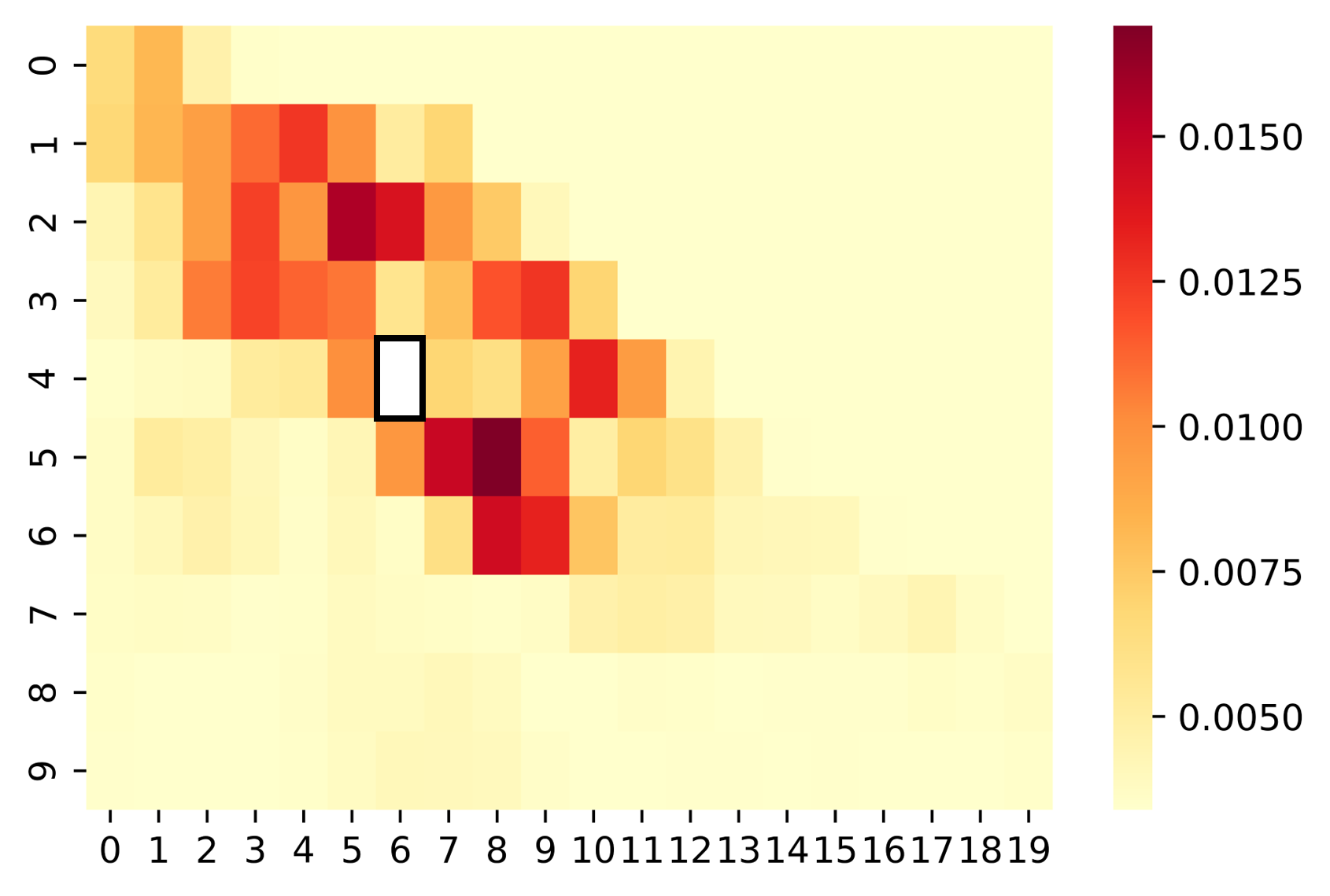
Much effort has been devoted to capturing the dependency between regions for traffic forecasting. While commendable, most works consider spatial and temporal dependency separately with independent processing modules [4, 5, 6, 7, 8, 9], which can hardly capture their joint nature in our current setting. Some recent works apply canonical Transformer [10] to capture region dependency [11, 12, 13, 14]. While impressive, canonical Transformer limits the training efficiency because it learns a region’s embedding as the weighted aggregation of all the other regions based on their computed attention scores. This results in computation complexity per layer, where is the number of regions. Moreover, it has been observed that the attention scores from the canonical Transformer have a long tail distribution [15]. We illustrate this in Figure 1 using a taxi dataset collected in New York City. We split New York City into regions and visualize the attention scores (after a SoftMax operation) between a target region (i.e., the region ) and other regions. Clearly, most regions have very small attention scores (i.e., the long-tail phenomenon), with the attention scores of more than of regions being less than 0.004. Such a long-tail effect may introduce noise for the region embedding learning and degrade the prediction performance.
We propose ST-TIS, a novel, small, efficient and accurate Spatial-Temporal Transformer with information fusion and region sampling for traffic forecasting. Given the historical (aggregated) inflow and outflow of regions from to , ST-TIS predicts the inflow and outflow of any region at , without relying on the transistion data between regions. With a small set of parameters, ST-TIS is efficient to train (offline phase). It extends the canonical Transformer with novel information fusion and region sampling strategies to learn the dynamic and possibly periodical spatial-temporal dependency between regions in a joint manner, hence achieving high prediction accuracy (online phase).
ST-TIS makes the following contributions:
-
•
A data-driven Transformer scheme for dynamic, possibly periodical, and joint spatial-temporal dependency learning. ST-TIS jointly considers the spatial-temporal dependencies between regions, rather than considering the two dependencies sequentially in a decoupled manner. In particular, ST-TIS considers the dynamic spatial-temporal dependency for any individual time slot with an information fusion module, and also the possibly periodical characteristic of spatial-temporal dependency from multiple time slots using an attention mechanism. Moreover, the dependency learning is data-driven, without any assumption on spatial locality. Due to its design, ST-TIS is small (in parameter footprint), fast (in training time), and accurate (in prediction).
-
•
A novel region sampling strategy for computationally efficient dependency learning. ST-TIS leverages the Transformer framework [10] to learn region dependency. To address the quadratic computation issue and mitigate the long-tail effect, it employs a novel region sampling strategy to generate a connected region graph and learns the dependency based on the graph. The dependencies between any pair of regions (both close and distant dependencies) are guaranteed to be considered in ST-TIS via information propagation, and the computational complexity is reduced from to , where is the number of regions.
-
•
Extensive experimental validation: We evaluate ST-TIS on two large-scale real datasets of taxi and bike sharing. Our results shows that ST-TIS is substantially more accurate than the state-of-the-art approaches, with a significant improvement in RMSE and MAPE (an average improvement of on RMSE, and on MAPE compared to STDN and DSAN). Furthermore, it is much more lightweight than most state-of-the-art models, and is ultra fast for training (with a reduction of on training time and on network parameters).
2 Related Works
Traffic forecasting has raised much attention in both academia and industry due to its social and commercial values. Some early traffic forecasting works propose using regression models, such as auto-regressive integrated moving average (ARIMA) models [16, 17, 18, 19] and non-parametric region models [20, 21]. All of these works consider temporal dependency, but they have not considered the spatial dependency between regions. Some other works extract features from heterogeneous data sources (e.g., POI, weather, etc.), and use machine learning models such as Support Vector Machine [22], Gradient Boosting Regression Tree [23], and linear regression model [24]. Despite of the encouraging results, they rely on manually defined features and have not considered the joint spatial-temporal dependency.
In recent years, deep learning techniques have been employed to study spatial and temporal correlations for traffic forecasting. Most existing works consider the spatial and temporal dependency in a decouple manner [4, 5, 6, 7, 8, 9], which can hardly capture their joint effect. For spatial dependency, Convolution Neural Network (CNN), Graph Neural Network (GNN), and Transformer have been widely applied. Regarding temporal dependency, Recurrent Neural Network (RNN) and its variants such as Long Short Term Memory (LSTM) and Gated Recurrent Unit (GRU) have been extensively studied. Compared with these works, ST-TIS considers the spatial and temporal dependency in a joint manner.
CNN has been applied in many works to capture dependencies between close regions [4, 5, 6, 7, 25]. In these works, a city is divided into some connected but non-overlapping grids, and the traffic in each grid is then predicted. However, these works cannot be used for fine-grained flow forecasting at an individual location [26], such as predicting flow for a docked bike-sharing station or a subway station. Moreover, CNN can hardly capture distant traffic dependency due to its relatively small receptive field [27, 28].
Some other works use GCN to capture spatial dependency [8, 9, 29, 30, 31, 32, 33, 34, 35]. In these works, a city is represented as a graph structure, and convolution operations are applied to aggregate spatially distributed information in the graph. In each aggregation layer, a region would aggregate the embedding of its neighbouring regions in the graph. However, these works highly rely on the graph structure for dependency learning. Prior works usually construct graphs based on the distance between regions or road network, based on the locality assumption (i.e., close regions have higher dependency). They have to stack more layers to learn dependency if the distance between two regions in the graph is long, and it ends up with an inefficient and over-smoothing model [31]. In recent years, Transformer [10] has been applied for traffic forecasting [11, 12, 13, 14]. The canonical Transformer can be seen as a special graph neural network with a complete graph, in which any pair of regions are connected. Consequently, the dependencies between both close and distant regions could be considered. Moreover, the self-attention mechanism and the network structure of Transformer have been demonstrated to be powerful in many prior works. However, the computational complexity of each aggregation round is for Transformer where is the number of regions, while that for GNN is where is the number of edges in the graph (). Furthermore, as a region may only have a strong dependency on a small portion of regions, aggregating the embedding of all regions would introduce noise and degrade its performance. In ST-TIS, we propose a region connected graph (i.e., there exists a path between any pair of regions in the graph), in which the degree of any node (i.e., region) is and the distance between any two regions in the graph is no more than . We extend the canonical Transformer with the proposed region connected graph, so that it can inherit the advantage of efficiency and effectiveness from both GNN and Transformer.
RNN and its variants such as LSTM and GRU [36, 37] have been used to capture temporal dependency [38, 6, 34, 35]. However, the performance of RNN-based models deteriorates rapidly as the length of the input sequence increases [39]. Some works incorporate the attention mechanism [40] to improve their capability of modeling long-term temporal correlations [29, 9, 7, 41]. Nevertheless, RNN-based networks are widely known to be difficult to train and are computationally intensive [8]. As recurrent networks generate the current hidden states as a function of the previous hidden state and the input for the position, they are in general more difficult to be trained in parallel. To address the issue, the self-attention mechanism is proposed as the replacement of RNN to model sequential data [10]. It has enjoyed success in capturing temporal correlations for traffic forecasting [42, 11, 12, 13]. Compared with RNN-based models, self-attention models can directly model long-term temporal interactions, but the computational complexity of using self-attention for temporal dependency learning in existing works is , where is the number of historical time slots. Compared with them, ST-TIS is conditional on the spatial-temporal dependency at any individual slot to generate weights for different time slots, so its computational complexity is in our work. In addition, the temporal dependency is jointly considered with the spatial dependency in ST-TIS, instead of in a decouple manner.
Some variants of Transformer have been proposed to address the efficiency issues of the canonical Transformer, such as LogSparse [43], Reformer [44], Informer [15], etc. While impressive, these approaches cannot be used in the scenario of capturing spatial-temporal dependency between regions for traffic forecasting we are considering in this work.
3 Preliminaries
3.1 Problem formulation
Definition 1.
(Region) The area (e.g., a city or subway route) is partitioned into non-overlapping regions. We use to denote the partitioned regions, in which denotes the -th region.
The way to partition an area is flexible for ST-TIS, e.g., grid map, road network, clustering, or train/bus/bike stations, etc.
Definition 2.
(Traffic data) We use and to denote the inflow and outflow data of all regions over time, respectively. Specifically, and is the inflow and outflow of the regions at time . Moreover, and is the inflow and outflow of region at time (i.e., the number of objects arriving at/departing from the region at time slot ). Furthermore, we use to denote the inflow of from to . Similarly, indicates the outflow of from to .
The formal formulation of the traffic forecasting problem is as follows:
Definition 3.
(Traffic Forecasting) Given the traffic data of regions from to , namely and , the traffic forecasting problem is to predict the inflow and outflow of any region at , namely and .
3.2 ST-TIS Overview
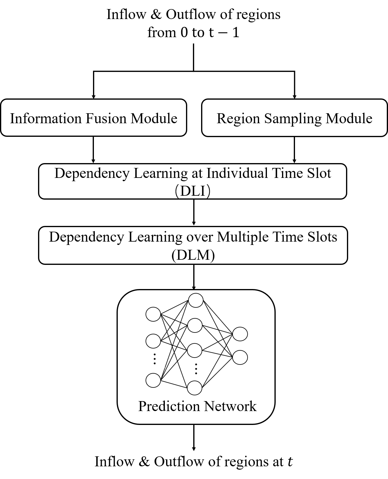
We overview the proposed ST-TIS in Figure 2. Given the traffic data of all regions from time slots to , ST-TIS is an end-to-end model to capture the spatial-temporal dependency and predict the inflow and outflow for any region at . There are five modules in ST-TIS. We explain the design goals and the relationship among modules as follows:
-
•
Information Fusion Module: A key to accurately predicting the traffic for regions is capturing the dynamic spatial-temporal (ST) dependency between regions in a joint manner. To this end, ST-TIS employs a information fusion module to learn the spatial-temporal-flow (STF) embedding by encoding its spatial, temporal, and flow information for any individual region at a time slot.
-
•
Region Sampling Module: To address the issues of quadratic computational complexity and long tail distribution of attention scores for the canonical Transformer, ST-TIS uses a novel region sampling strategy to generate a region connected graph. The dependency learning would be based on the generated graph.
-
•
Dependency Learning for Individual Time Slot (DLI): Given the STF embedding at a time slot and the region connected graph, ST-TIS extends the canonical Transformer to jointly capture the dynamic spatial-temporal dependency between regions at the time slot. As the spatial and temporal information has been both encoded in the STF embedding, the joint effect of spatial-temporal dependencies between regions could be captured. Moreover, with the region connected graph, only the attention scores between neighbouring nodes (i.e., regions) are computed, and only the embedding of one’s neighbouring regions are aggregated. Dependency between non-neighbouring nodes is considered via information propagation between multiple layers in the network. Consequently, it cuts the computational complexity of a layer from to where is the number of regions, and addresses the issue of the long-tail effect for dependency learning.
-
•
Dependency Learning over Multiple Time Slots (DLM): Given the region embedding from DLI at multiple time slots, DLM captures the periodic patterns of spatial-temporal dependency using the attention mechanism. The influence of spatial-temporal dependency at historical time slots on the predicted time slot is hence considered in ST-TIS. The learning process is data-driven, without any prior assumption of traffic periods.
-
•
Prediction Network (PN): Given the results from DLM, ST-TIS uses a fully connected neural network to predict the inflow and outflow of regions ( and ) simultaneously.
4 ST-TIS Details
We present the details of ST-TIS in this section. We first elaborate the information fusion module in Section 4.1, followed by the region sampling module in Section 4.2. After that, we introduce the dependency learning for individual time slot (DLI) in Section 4.3, and the dependency learning over multiple time slots (DLM) in Section 4.4. Finally, we present the prediction network (PN) in Section 4.5.
4.1 Information Fusion Module
To capture the dynamic joint spatial-temporal dependency for traffic forecasting, it is essential to fuse the spatial-temporal information for each region at any individual time slot. To this end, ST-TIS employs the information fusion module to learn one’s spatial-temporal-flow (STF) embedding by fusing its position, time slot, and flow information.
Given regions, we first use a one-hot vector to represent a region , in which only the -th element in is and otherwise . After that, we encode the position information for a region as follows,
| (1) |
where is the spatial embedding of , and are learnable parameters, and is a hyperparameter.
In terms of temporal information, we first split a day into time slots and represent the -th time slot using a one-hot vector . After that, we learn the temporal embedding by
| (2) |
where is the temporal embedding of the -th time slot in a day, and are learnable parameters.
Recall that the traffic of one region at may depend on that of another region at previous time slots due to the travel time between two regions. Thus, we use one’s surrounding observations instead of solely using a snapshot to learn the dependency [43]. We define the surrounding observations of a region at a time slot as follows:
Definition 4.
(Surrounding observations) For a region at a time slot , its surrounding observations are defined as the flow in the previous time slots: .
Note that by employing the surrounding observations, the temporal lag of the dependency between regions could be considered. Given the surrounding observations of at , we first apply the 1-D convolution of kernel size () with stride and output channels on its inflow and outflow surrounding observations to extract different patterns. The flow embedding of at is computed as
| (3) |
where is the concatenation operation, and are the convolutional operation for inflow and outflow data respectively, , are learnable parameters, and .
Finally, we fuse the position, time slot and flow information to learn the STF embedding of a region at time . We define that is the -th time slot in a day, where is an matching function. The fusion process is defined as
| (4) |
where is the STF embedding, and are learnable parameters.
4.2 Region Sampling
To capture a region’s dependency on others (both nearby and distant), a canonical Transformer computes the attention scores between the target region and all other regions, and aggregats the embedding of all other regions based on the computed attention scores. However, this results in the issues of quadratic computation and long-tail effect for dependency learning.
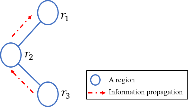
Fortunately, prior works have showed that information could be propogated between nodes in a graph via a multi-layer network structure [45]. Hence, with a proper graph structure and network structure, a region can aggregate the embedding of another even without directly evaluating their attention score. We present a toy example in Figure 3, in which regions are represented as nodes in the graph and connected with egdes. In the first aggregation layer, would capture the information from , while would capture the information from . Since the information of has been aggregated in , could also capture it in the second aggregation layer without computing the attention score between and . From this example, we conclude that a node’s information can reach another with a -layer aggregation operation if their distance is not more than in the graph.
To address the limitations of the canonical Transformer, we propose to generate a connected graph (i.e., there exists at least a path between any two nodes in the graph), in which the degree of any node (i.e., region) is not more than and the distance between any pair of nodes are not more than 2. In this way, for a target region, we only have to aggregate the embedding of regions in an aggregation layer, and the influence from other regions can be captured in a two-layer aggregation process by information propagation. With such design, we do not have to compute the attention scores between any pairs of regions and aggregate the embedding of all regions for a target region, so that the computation complexity is reduced to for each layer, and the long-tail issue is also addressed.
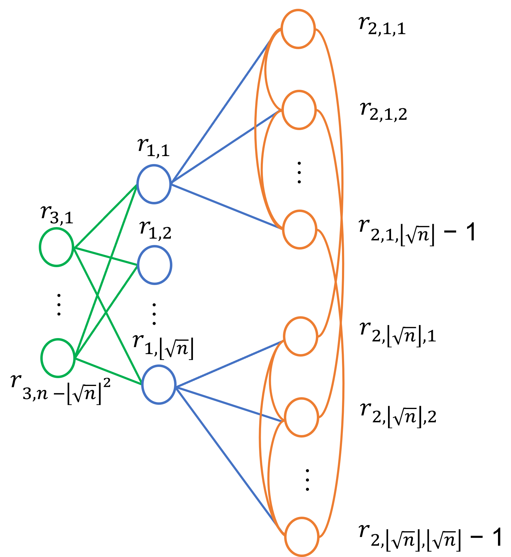
In this work, we present a heuristic approach for region connected graph generation. We first calculate the traffic similarity between any pair of regions. The calculation of the traffic similarity is flexible and it could be any similarity metric. As an example, we use DTW in this work to measure the similarity in terms of the average traffic over time slots of a day. We use to represent the similarity matrix, in which is the similarity between and . Based on , the process of the connected graph generation is illustrated in Figure 4.
We first select top regions without replacement, which have the largest sum of similarity with other regions, represented as , . For any region , we then select regions without replacement, which have the largest similarity between them and , represented as , and we connect to (). After that, we connect a region to regions and , where and . Finally, if , the remaining regions woule be connected to where , represented as . If , we randomly select a region from , and connect it to , where , represented as .
Theorem 1.
The degree of any node in the region connected graph is , and the distance between any two nodes in the graph is less than .
Proof.
The generation of the region connected graph ensures that a node is connected to at most other nodes, and hence the degree is .
The distance of (or ) and is both , where , , and . Thus, the distance between (or ) and any other region is no more than in the graph.
For region , since the distance of and is both 1 where and , the distance of is hence 2. Thus, the distance between and any other region is also no more than .
In terms of , as the distance of and is 1, where and , the distance between and any other regions is hence no more than . Therefore, the distance between any two regions in the graph is less than . ∎
Because the distance between any two regions in the proposed graph is less than , the dependencies between any two regions could be considered if the layer number of the aggregation network is larger than .
4.3 Dependency Learning for Individual Time Slot (DLI)
Given the STF embedding of regions for time and the generated region connected graph, ST-TIS captures the spatial-temporal dependencies between regions based on an extended Transformer encoder. Following the canonical Transformer, ST-TIS employs an multi-head attention mechanism, so that it could account for different dependencies between regions. For the -th head, the attention score between and at is defined as
| (5) |
where and are the STF embedding of regions and at (Equation 4), and are learnable parameters, and is a hyperparameter for the embedding size.
Unlike the canonical Transformer, we do not evaluate the attention scores between one region and all other regions. Instead, we only compute one’s attention scores with its neighbouring regions in the region connected graph, and aggregate their embedding in terms of their attention score to update the region’s embedding. For the -th head, the embedding of a region at time is then updated as
| (6) |
where is the output of the -th head, is the neighbouring regions of in the graph, is the attention score defined in Equation 5. As the degree of any node is , the computation complexity of attention score evaluation and embedding aggregation is hence for all regions in a layer.
Finally, we concatenate the results of multi-heads and the embedding of is computed as
| (7) |
where is the concatenation operation, is the embedding of , are learnable parameters and is the number of heads.
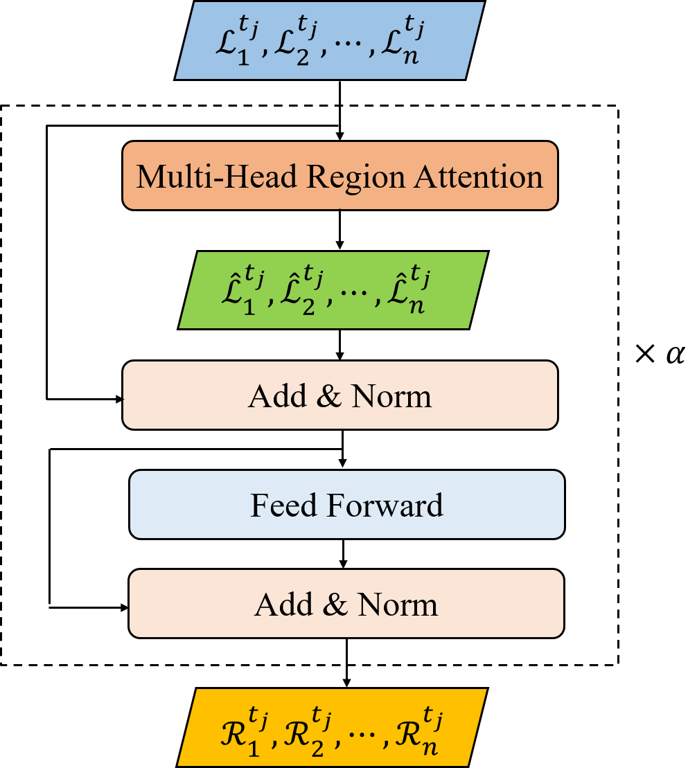
Following the structure of Transformer[10], the output of the multi-head region attention layers is then passed to a fully connected neural network (Figure 5). We also employ a residual connection between each of the two layers. As we discussed in Section 4.2, the information propagation is achieved with a multi-layer network structure. Thus, we stack the layers times (the effect of will be discussed in Section 5.7). We denote the final output of the DLI as , where is the embedding of region at .
Compared with the canonical Transformer, we only need to compute the attention scores and aggregate the embedding between adjacent nodes in the region connected graph. The computation complexity is hence reduced from to for each layer.
4.4 Dependency Learning over Multiple Time Slots (DLM)
Considering the spatial-temporal dependency may have periorical characteristic, DLM learns the periodic dependency by evaluating the correlation between and the dependency at other historical time slots (where ). After that, it generates a new embedding for by aggregating the embedding at different time slots according to their correlations.
Specifically, we consider the short-term and long-term period for traffic data in this work. The spatial-temporal dependency at the following historical time slots are used as the model input to predict the inflow and outflow of regions at : spatial-temporal dependency in the recent time slots (i.e., short-term period); the same time interval in the recent days (i.e.,long-term period).
We employ a point-wise aggregation with self-attention to evaluate their correlations and aggregate the embedding accordingly. To capture the multiple periodic dependency, we use an multi-head attention network in DLM.
Given a set of historical time slot , the -th dependency on a historical time slot is calculated as follows:
| (8) |
where and are learnable parameters.
We use a softmax function to normalize the dependency and aggregate the context of each time slot by weight:
| (9) |
The aggregation of the -th head is hence
| (10) |
where is the set of historical time slots, is the aggregation result of the -th head, and are learnable parameters. Finally, we concatenate the results of different heads with
| (11) |
where is the concatenation operation, and are learnable parameters. We then pass to a fully connected neural network to obtain the spatial-temporal embedding of at . Note that we also employ a residual connection between each of the two layers to avoid gradient exploding or vanishing. The output of the DLM is denoted as for region at .
Different from prior works, the periodic dependency learning is conditional on the spatial-temporal dependency at each individual time slot. Consequently, the spatial and temproal dependencies are jointly considered during the periodic dependency learning. The computation complexity is , where is the number of historical time slots used for learning.
4.5 Prediction Network (PN)
Given the spatial-temporal embedding of a region, the prediction network predicts the inflow and outflow using the fully connected network. The forecasting function is defined as
| (12) |
where and is the forecasting inflow and outflow respectively, is the ReLU activation function and , and are learnable parameters.
We simultaneously forecast the inflow and outflow in our work, and define the loss function as follows:
| (13) |
where is the number of regions.
5 Illustrative Experimental Results
In this section, we first introduce the datasets and the data processing approaches in Section 5.1, and the evaluation metrics and baseline approaches in Section 5.2. Then, we compare the accuracy and training efficiency of ST-TIS with the state-of-the-art methods in Sections 5.3 and 5.4, respectively. After that, we evaluate the performance of variants of ST-TIS and the effect of surrounding observations in Sections 5.6 and 5.5, respectively, followed by the discussion on the hyperparameters of layer number in Section 5.7 and head number in Section 5.8.
5.1 Datasets
We conduct extensive traffic study and model evaluations based on two real-world traffic flow datasets collected in New York City (NYC), the NYC-Taxi dataset and the NYC-Bike dataset. Each dataset contains trip records, each of which consists of origin, destination, departure time, and arrival time. The NYC-Taxi dataset contains taxi trip records of NYC in 2015, from 01/01/2015 to 03/01/2015. The NYC-Bike dataset was collected from the NYC Citi Bike system from 07/01/2016 to 08/29/2016, and contains trip records.
The city is split into regions with a size of kmkm. The time interval is set as minutes for both datasets. The two datasets were pre-processed and released online111https://github.com/tangxianfeng/STDN/blob/master/data.zip by the prior work [7].
In both of the taxi dataset and bike dataset, we use data from the previous days as the training data, and the remaining days as the testing data. In the training data, we select of the training data to train our model and the remaining for validation. We use the Min-Max normalization to rescale the range of volume value in , and recover the result for evaluation after forecasting. In our experiments, we exclude the results of those regions the inflow or outflow of which is less than 10 when evaluating the model. It is a common practice used in industry and many prior works [6, 7, 42].
5.2 Performance Metrics and Baseline Methods
We use Root Mean Squared Errors (RMSE) and Mean Average Percentage Error (MAPE) as the evaluation metrics, which are defined as follows:
| (14) |
| (15) |
where and are the ground-truth and forecasting result of the -th sample, and is the total number of samples.
| Dataset | Method | Inflow | Outflow | ||
|---|---|---|---|---|---|
| RMSE | MAPE | RMSE | MAPE | ||
| NYC-Taxi | HA | 33.83 | 21.14% | 43.82 | 23.18% |
| ARIMA | 27.25 | 20.91% | 36.53 | 22.21% | |
| Ridge | 24.38 | 20.07% | 28.51 | 19.94% | |
| XGBoost | 21.72 | 18.70% | 26.07 | 19.35% | |
| MLP | 22.080.50 | 18.310.83% | 26.670.56 | 18.430.62% | |
| ConvLSTM | 23.670.20 | 20.700.20% | 28.130.25 | 20.500.10% | |
| ST-ResNet | 21.630.25 | 21.090.51% | 26.230.33 | 21.130.63% | |
| STDN | 19.050.31 | 16.250.26% | 24.100.25 | 16.300.23% | |
| ASTGCN | 22.050.37 | 20.250.26% | 26.100.25 | 20.300.31% | |
| STGODE | 21.460.42 | 19.220.36% | 27.240.46 | 19.300.34% | |
| STSAN | 23.070.64 | 22.241.91% | 27.830.30 | 25.901.67% | |
| DSAN | 18.320.39 | 16.070.31% | 24.270.30 | 17.700.35% | |
| ST-TIS | 17.730.23 | 14.650.32% | 21.960.13 | 14.830.76% | |
| NYC-Bike | HA | 11.93 | 27.06% | 12.49 | 27.82% |
| ARIMA | 11.25 | 25.79% | 11.53 | 26.35% | |
| Ridge | 10.33 | 24.58% | 10.92 | 25.29% | |
| XGBoost | 8.94 | 22.54% | 9.57 | 23.52% | |
| MLP | 9.120.24 | 22.400.40% | 9.830.19 | 23.120.24% | |
| ConvLSTM | 9.220.19 | 23.200.47% | 10.400.17 | 25.100.45% | |
| ST-ResNet | 8.850.13 | 22.980.53% | 9.800.12 | 25.060.36% | |
| STDN | 8.150.15 | 20.870.39% | 8.850.11 | 21.840.36% | |
| ASTGCN | 9.050.31 | 22.250.36% | 9.340.24 | 23.130.30% | |
| STGODE | 8.580.38 | 23.330.26% | 9.230.31 | 23.990.23% | |
| STSAN | 8.200.45 | 20.421.33% | 9.870.23 | 23.870.71% | |
| DSAN | 7.970.25 | 20.230.18% | 10.070.58 | 23.920.39% | |
| ST-TIS | 7.570.04 | 18.640.23% | 7.730.10 | 18.580.19% | |
We compare our model with the following state-of-the-art approaches:
-
•
Historical average (HA): It uses the average of traffic at the same time slots in historical data for prediction.
-
•
ARIMA: It is a conventional approach for time series data forecasting.
-
•
Ridge Regression: A regression approach for time series data forecasting.
-
•
XGBoost [46]: A powerful approach for building supervised regression models.
-
•
Multi-Layer Perceptron (MLP): A three-layer fully-connected neural network.
-
•
Convolutional LSTM (ConvLSTM) [47]: It is a special recurrent neural network with a convolution structure for spatial-temporal prediction.
-
•
ST-ResNet [5]: It uses multiple convolutional networks with residual structures to capture spatial correlations from different temporal periods for traffic forecasting. It also considers external data such as weather, holiday events, and metadata.
-
•
STDN [7]: It considers the dynamic spatial correlation and temporal shifted problem using the combination of CNN and LSTM. External data such as weather and event are considered in the work.
-
•
ASTGCN [48]: It is an attention-based spatial-temporal graph convolutional network (ASTGCN) model to solve traffic flow forecasting problem.
-
•
STGODE [31]: It uses a spatial-temporal graph ordinary differential equation network to predict traffic flow based on two predefine graph, namely a spatial graph in terms of distance, and a semantic graph in terms of flow similarity.
-
•
STSAN [12]: It uses CNN to capture spatial information and the canonical Transformer to consider the temporal dependencies over time. In particular, transition data between regions are used to indicate the correlation between regions.
-
•
DSAN [13]: It uses the canonical Transformer to capture the spatial-temporal correlations for spatial-temporal prediction, in which transition data between regions are used for correlation modeling.
We use the identical datasets and data process approach as the work STDN [7], and use the results of the work [7] as the benchmark for discussion. The experiment results of (1) (8) in Table I are reported in the work [7]. The evaluation of ASTGCN, STGODE, STSAN, and DSAN is based on the code from their authors’ GitHubs.
We implement our model using PyTorch. Data and code can be found in https://github.com/GuanyaoLI/ST-TIS. We use the following data as the model input since they achieve the best performance on the validation datasets: data in the recent past 3 hours (i.e., as the slot duration is minutes); the same time slot in the recent past 10 days (i.e., ). The other default hyperparameter settings are as follows. The default length of the surrounding observations is (i.e. hours), the number of convolution kernels is , and the dimension is set as . The number of for DLI in Figure 5 is set as , and the number of heads is set as for the two modules. Furthermore, the dropout rate is set as , the learning rate is set as , and the batch size is set to be . Adam optimizer is used for model training. We trained our model on a machine with a NVIDIA RTX2080 Ti GPU.
5.3 Prediction Accuracy
We compared the accuracy of ST-TIS with the state-of-the-art methods using the metrics RMSE and MAPE. The results for the two datasets are presented in Table I. Each approach was run times, and the mean and standard deviation are reported. As shown in the table, ST-TIS significantly outperforms all other approaches on both metrics and datasets.
Specifically, the performance of the conventional time series forecasting approaches (HA and ARIMA) is poor for both datasets because these approaches do not consider the spatial dependency. Conventional machine learning approaches (Ridge, XGBoost, and MLP), which consider spatial dependency as features, have better performance than HA and ARIMA. However, they fail to consider the joint spatial-temporal dependencies between regions. Most deep learning-based models have further improvements than conventional works, illustrating the ability of deep neural networks to capture the complicated spatial and temporal dependency. ST-TIS is substantially more accurate than state-of-the-art approaches (i.e., ConvLSTM, STResNet, STDN, ASTGCN and STGODE). For example, it has an average improvement of on RMSE and on MAPE compared to STDN and DSAN. The reasons for the improvements are that it can capture the correlations between both nearby and distant regions, and it considers the spatial and temporal dependency in a joint manner. We find that the improvement is more significant on the NYC-Taxi dataset than on the NYC-Bike dataset. The reason could be that people prefer using taxis instead of bikes for long-distance travel, and so the correlations with distant regions are more important for the prediction task on the taxi dataset. The significant improvement demonstrates that ST-TIS has a better ability to capture the correlations for distant regions than the other approaches which have the spatial locality assumption. ST-TIS also outperforms other Transformer-based approaches (such as STSAN and DSAN). The reason is that with the information fusion and region sampling strategies in ST-TIS, the long-tail issue of the canonical Transformer is addressed and the joint spatial-temporal correlations are considered. The significant improvements demonstrate the effectiveness of our proposed model.
5.4 Training Efficiency
| Dataset | Method |
|
Total time (s) | ||
|---|---|---|---|---|---|
| NYC-Taxi | ST-ResNet | 7.31 | 3077.51 | ||
| STDN | 445.47 | 34746.66 | |||
| ASTGCN | 25.31 | 6272.88 | |||
| STGODE | 18.53 | 3423.48 | |||
| STSAN | 426.75 | 33769.32 | |||
| DSAN | 386.17 | 29390.75 | |||
| ST-TIS | 10.21 | 1231.5 | |||
| NYC-Bike | ST-ResNet | 7.25 | 2921.75 | ||
| STDN | 480.21 | 23066.43 | |||
| ASTGCN | 25.68 | 5084.64 | |||
| STGODE | 18.76 | 3752.89 | |||
| STSAN | 426.28 | 31216.28 | |||
| DSAN | 434.03 | 26476.20 | |||
| ST-TIS | 10.37 | 1556.8 |
Training and deploying large deep learning models is costly. For example, the cost of trying combinations of different hyper-parameters for a large model is computationally expensive and it highly relies on training resources [3]. Thus, we compare the training efficiency of ST-TIS with some state-of-the-art deep learning based approaches (i.e., ST-ResNet, STDN, ASTGCN, STGODE, STSAN, and DSAN) in terms of training time and number of learnable parameters.
The results of the average training time per epoch and the total training time are presented in Table II.
| Method | Number of parameters |
|---|---|
| ST-ResNet | 4,917,041 |
| STDN | 9,446,274 |
| ASTGCN | 450,031 |
| STGODE | 433,073 |
| DSAN | 1,621,634 |
| STSAN | 34,327,298 |
| ST-TIS | 139,506 |
ST-ResNet achieves the least training time among all comparison approaches because it solely employs simple CNN and does not rely on RNN for temporal dependency learning. The average time per epoch of ST-TIS is close to ST-ResNet. In addition, ST-TIS is trained significantly faster than other approaches (with a reduction of ). STDN uses LSTM to capture temporal correlation, which is in general more difficult to be trained in parallel. STSAN and DSAN also employ Transformer with self-attention for spatial and temporal correlation learning, but our proposed approach is significantly efficient than them, illustrating the efficiency of the proposed region graph for model training.
Furthermore, we also compare the number of learnable parameters of each model in Table III. More parameters may lead to difficulties in model training, and it requires more memory and training resources. Compared with other state-of-the-art approaches, ST-TIS is much more lightweight with fewer parameters for training (with a reduction of ). The comparison results in Tables I, II and III demonstrate that our proposed ST-TIS is faster and more lightweight than other deep learning based baseline approaches, while achieving even better prediction accuracy.
5.5 Design Variations of ST-TIS
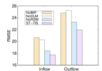
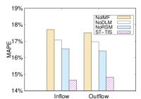
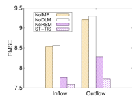
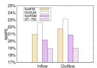
We compare ST-TIS with its variants to evaluate the effectiveness of the proposed modules. The following variants are discussed:
-
•
NoIFM: We remove the information fusion module from ST-TIS. Only the surrounding observation of a time slot is used as the input of the model instead of the fusion result.
-
•
NoRSM: We remove the region sampling module from ST-TIS. The canonical Transformer is used to capture the dependencies between regions without region sampling.
-
•
NoDLM: We remove the module of dependency learning over multiple time slots, and only use as the input of the prediction network for prediction.
The RMSE and MAPE on the NYC-Taxi dataset are presented in Figures 6(a) and 6(b), respectively. After taking the information fusion module away, the performance degrades significantly. The reason is that the information fusion module plays a fundermental role in jointly considering the spatial-temporal dependency. Without such module, our approach would degenerate to consider the spatial and temporal dependency in a decouple manner. The experimental results demonstrate the importance of considering spatial-temporal dependency jointly and the effective of the proposed information fusion module. Moreover, without the region sampling module, our approach still achieve a good prediction performance because the canonical Transformer is good at capturing dependencies between regions. The performance is further improved with the region sampling since it could address the long-tail issue of the canonical Transformer for embedding aggregation. Furthermore, the RMSE and MAPE increase when the periodical characteristic of spatial-temporal dependency is not considered (i.e., NoDLM), which indicates the necessity of considering the period of spatial-temporal dependency and demonstrates the effectiveness and rationality of our model design. Similar and consistent findings can be observed on the NYC-Bike dataset in Figures 7(a) and 7(b).
5.6 Surrounding Observations
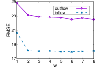
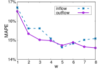
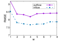
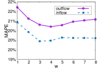
Recall that the dependency between two regions may have temporal lagging due to the travel time between them. To capture such lagging dependency, ST-TIS uses the surrounding observations to learn the region correlations for each time slot, which contains the inflow and outflow in the previous time slots. We thus evaluate the impact of on the performance of our model.
Figures 8(a) and 8(b) show the RMSE and MAPE versus different lengths on the NYC-Taxi dataset. A larger length indicates that more information is encoded from the surrounding observations. When , only the observation at a time slot is used for dependency learning, and the model fails to capture the lagging characteristic of dependency. As the length increases, the RMSE and MAPE of both inflow and outflow forecasting decrease (). The performance improvement demonstrates the importance of using the surrounding observations to learn the dependencies between regions. RMSE and MAPE increase slightly but remain stable when the length is large (). The potential reason is that, when is larger than the travel time between regions, increasing would not introduce more information for dependency learning. On the other hand, a larger may introduce some noise and more parameters for the model, leading to difficulties in model training [13]. The RMSE and MAPE versus different lengths of surrounding observations on the NYC-Bike dataset are shown in Figures 9(a) and 9(b), which are consistent with the results for the NYC-Taxi dataset. When the length is small (), RMSE and MAPE decrease as the length becomes larger, but they slightly increase when the length is large ().
5.7 Layer Number
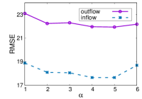
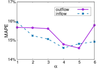
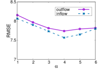
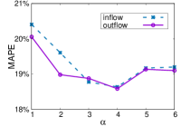
In ST-TIS, DLI is stacked times to ensure the information propagtion between regions and improve the model robustness. We evaluate the effect of on the prediction performance using RMSE and MAPE. The results for the taxi dataset are presented in Figure 10. When , only the dependencies on one’s neighbouring regions in the graph are considering, resulting in the worst prediction accuracy. When , the dependencies on all other regions could be captured. We find that with the layer number increases, the RMSE and the MAPE declines for both inflow and outflow, indicating the performance improvement. However, we find that when the layer number is too large ( in our experiments), the performance on RMSE and MAPE degrades, because too many layers may result in difficulties of model training. Similar results are observed on the bike dataset (Figure 11).
5.8 Head Number
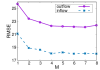
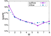
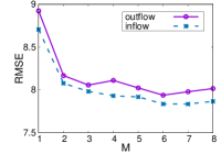
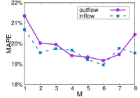
We use the multi-head attention mechanism in ST-TIS for dependency learning, so that different heads could capture different patterns from the historical data. In our experiments, we evaluate the impact of the head number on the prediction performance. The results of RMSE and MAPE versus the head number on the taxi and bike datasets are presented in Figures 12 and 13, respectively. As shown in Figures 12(a) and 13(a), with the head number increases, the RMSE on the two datasets declines, demonstrating the multi-head mechanism could benefit the dependency learning and improve the prediction accuracy. We also observe that when the head number become larger ( on the taxi dataset while on the bike dataset), the improvements are not significant. The reason could be that some heads may focus on the same pattern when there are many heads. In terms of MAPE, similar findings could be observed in Figures 12(b) and 13(b). Moreover, the MAPE increases slightly when the head number becomes large (). It is because increasing the head number leads to more learnable parameters, which would result in difficulties for model training.
6 Conclusion
We propose ST-TIS, a novel, small (in parameters), computationally efficient and highly accurate model for traffic forecasting. ST-TIS employs a spatial-temporal Transformer with information fusion and region sampling to jointly consider the dynamic spatial and temporal dependencies between regions at any individual time slots, and also the possibly periodic spatial-temporal dependency from multiple time slots. In particular, ST-TIS boosts the efficiency and addresses the long-tail issue of the canonical Transformer using a novel region sampling strategy, which reduces the complexity from to , where is the number of regions. We have conducted extensive experiments to evaluate ST-TIS, using a taxi and a bike sharing datasets. Our experimental results show that ST-TIS significantly outperforms the state-of-the-art approaches in terms of training efficiency (with a reduction of on training time and on network parameters), and hence is efficient in tuning, training and memory. Despite its small size and fast training, it achieves higher accuracy in its online predictions than other state-of-the-art works (with improvement of up to on RMSE, and on MAPE).
References
- [1] Y. Zheng, L. Capra, O. Wolfson, and H. Yang, “Urban computing: concepts, methodologies, and applications,” ACM Transactions on Intelligent Systems and Technology (TIST), vol. 5, no. 3, pp. 1–55, 2014.
- [2] W. Jiang and J. Luo, “Graph neural network for traffic forecasting: A survey,” arXiv preprint arXiv:2101.11174, 2021.
- [3] G. Menghani, “Efficient deep learning: A survey on making deep learning models smaller, faster, and better,” arXiv preprint arXiv:2106.08962, 2021.
- [4] J. Zhang, Y. Zheng, D. Qi, R. Li, and X. Yi, “Dnn-based prediction model for spatio-temporal data,” in Proceedings of the 24th ACM SIGSPATIAL International Conference on Advances in Geographic Information Systems. California, USA: ACM, 2016, pp. 1–4.
- [5] J. Zhang, Y. Zheng, and D. Qi, “Deep spatio-temporal residual networks for citywide crowd flows prediction,” in Thirty-First AAAI Conference on Artificial Intelligence. California USA: AAAI, 2017, pp. 1655 – 1661.
- [6] H. Yao, F. Wu, J. Ke, X. Tang, Y. Jia, S. Lu, P. Gong, J. Ye, and Z. Li, “Deep multi-view spatial-temporal network for taxi demand prediction,” in Thirty-Second AAAI Conference on Artificial Intelligence. Louisiana, USA: AAAI, 2018, pp. 2588 – 2595.
- [7] H. Yao, X. Tang, H. Wei, G. Zheng, and Z. Li, “Revisiting spatial-temporal similarity: A deep learning framework for traffic prediction,” in Proceedings of the AAAI Conference on Artificial Intelligence, vol. 33. New York, USA: AAAI, 2019, pp. 5668–5675.
- [8] B. Yu, H. Yin, and Z. Zhu, “Spatio-temporal graph convolutional networks: a deep learning framework for traffic forecasting,” in Proceedings of the 27th International Joint Conference on Artificial Intelligence. Stockholm, Sweden: IJCAI, 2018, pp. 3634–3640.
- [9] X. Geng, Y. Li, L. Wang, L. Zhang, Q. Yang, J. Ye, and Y. Liu, “Spatiotemporal multi-graph convolution network for ride-hailing demand forecasting,” in Proceedings of the AAAI Conference on Artificial Intelligence, vol. 33. Hawaii, USA: AAAI, 2019, pp. 3656–3663.
- [10] A. Vaswani, N. Shazeer, N. Parmar, J. Uszkoreit, L. Jones, A. N. Gomez, Ł. Kaiser, and I. Polosukhin, “Attention is all you need,” in Advances in neural information processing systems. Long Beach, CA, USA: ACM, 2017, pp. 5998–6008.
- [11] Y. Zhou, J. Li, H. Chen, Y. Wu, J. Wu, and L. Chen, “A spatiotemporal attention mechanism-based model for multi-step citywide passenger demand prediction,” Information Sciences, vol. 513, pp. 372–385, 2020.
- [12] H. Lin, W. Jia, Y. You, and Y. Sun, “Interpretable crowd flow prediction with spatial-temporal self-attention,” arXiv preprint arXiv:2002.09693, vol. [cs.LG], 2020.
- [13] H. Lin, R. Bai, W. Jia, X. Yang, and Y. You, “Preserving dynamic attention for long-term spatial-temporal prediction,” in Proceedings of the 26th ACM SIGKDD International Conference on Knowledge Discovery & Data Mining. Virtual Conference: ACM, 2020, pp. 36–46.
- [14] M. Xu, W. Dai, C. Liu, X. Gao, W. Lin, G.-J. Qi, and H. Xiong, “Spatial-temporal transformer networks for traffic flow forecasting,” arXiv preprint arXiv:2001.02908, 2020.
- [15] H. Zhou, S. Zhang, J. Peng, S. Zhang, J. Li, H. Xiong, and W. Zhang, “Informer: Beyond efficient transformer for long sequence time-series forecasting,” in Proceedings of AAAI, 2021.
- [16] S. Shekhar and B. M. Williams, “Adaptive seasonal time series models for forecasting short-term traffic flow,” Transportation Research Record, vol. 2024, no. 1, pp. 116–125, 2007.
- [17] B. Pan, U. Demiryurek, and C. Shahabi, “Utilizing real-world transportation data for accurate traffic prediction,” in 2012 IEEE 12th International Conference on Data Mining. Brussels, Belgium: IEEE, 2012, pp. 595–604.
- [18] L. Moreira-Matias, J. Gama, M. Ferreira, J. Mendes-Moreira, and L. Damas, “Predicting taxi–passenger demand using streaming data,” IEEE Transactions on Intelligent Transportation Systems, vol. 14, no. 3, pp. 1393–1402, 2013.
- [19] A. Abadi, T. Rajabioun, and P. A. Ioannou, “Traffic flow prediction for road transportation networks with limited traffic data,” IEEE transactions on intelligent transportation systems, vol. 16, no. 2, pp. 653–662, 2014.
- [20] B. L. Smith, B. M. Williams, and R. K. Oswald, “Comparison of parametric and nonparametric models for traffic flow forecasting,” Transportation Research Part C: Emerging Technologies, vol. 10, no. 4, pp. 303–321, 2002.
- [21] R. Silva, S. M. Kang, and E. M. Airoldi, “Predicting traffic volumes and estimating the effects of shocks in massive transportation systems,” Proceedings of the National Academy of Sciences, vol. 112, no. 18, pp. 5643–5648, 2015.
- [22] Y. Zhang and Y. Xie, “Forecasting of short-term freeway volume with v-support vector machines,” Transportation Research Record, vol. 2024, no. 1, pp. 92–99, 2007.
- [23] Y. Li, Y. Zheng, H. Zhang, and L. Chen, “Traffic prediction in a bike-sharing system,” in Proceedings of the 23rd SIGSPATIAL International Conference on Advances in Geographic Information Systems. Seattle, Washington: ACM, 2015, pp. 1–10.
- [24] Y. Tong, Y. Chen, Z. Zhou, L. Chen, J. Wang, Q. Yang, J. Ye, and W. Lv, “The simpler the better: a unified approach to predicting original taxi demands based on large-scale online platforms,” in Proceedings of the 23rd ACM SIGKDD international conference on knowledge discovery and data mining. Halifax, NS, Canada: ACM, 2017, pp. 1653–1662.
- [25] T. Li, J. Zhang, K. Bao, Y. Liang, Y. Li, and Y. Zheng, “Autost: Efficient neural architecture search for spatio-temporal prediction,” in Proceedings of the 26th ACM SIGKDD International Conference on Knowledge Discovery & Data Mining. Virtual Conference: ACM, 2020, pp. 794–802.
- [26] S. He and K. G. Shin, “Towards fine-grained flow forecasting: A graph attention approach for bike sharing systems,” in Proceedings of The Web Conference 2020. Taiwan: ACM, 2020, pp. 88–98.
- [27] H. Yao, C. Zhang, Y. Wei, M. Jiang, S. Wang, J. Huang, N. V. Chawla, and Z. Li, “Graph few-shot learning via knowledge transfer,” in Thirty-Forth AAAI Conference on Artificial Intelligence. New York, USA: AAAI, 2020, pp. 6656 – 6663.
- [28] G. Li, M. Muller, A. Thabet, and B. Ghanem, “Deepgcns: Can gcns go as deep as cnns?” in Proceedings of the IEEE International Conference on Computer Vision. Seoul, Korea: IEEE, 2019, pp. 9267–9276.
- [29] Z. Pan, Y. Liang, W. Wang, Y. Yu, Y. Zheng, and J. Zhang, “Urban traffic prediction from spatio-temporal data using deep meta learning,” in Proceedings of the 25th ACM SIGKDD International Conference on Knowledge Discovery & Data Mining. Anchorage, AK, USA: ACM, 2019, pp. 1720–1730.
- [30] X. Wang, Y. Ma, Y. Wang, W. Jin, X. Wang, J. Tang, C. Jia, and J. Yu, “Traffic flow prediction via spatial temporal graph neural network,” in Proceedings of The Web Conference 2020. Taiwan: ACM, 2020, pp. 1082–1092.
- [31] Z. Fang, Q. Long, G. Song, and K. Xie, “Spatial-temporal graph ode networks for traffic flow forecasting,” in Proceedings of the 27th ACM International Conference on knowledge Discovery and Data Mining. Singapore: ACM, 2021.
- [32] M. Li and Z. Zhu, “Spatial-temporal fusion graph neural networks for traffic flow forecasting,” in Proceedings of the 27th ACM International Conference on knowledge Discovery and Data Mining. Singapore: ACM, 2021.
- [33] C. Song, Y. Lin, S. Guo, and H. Wan, “Spatial-temporal synchronous graph convolutional networks: A new framework for spatial-temporal network data forecasting,” in Proceedings of the AAAI Conference on Artificial Intelligence, vol. 34, no. 01, 2020, pp. 914–921.
- [34] H. Shi, Q. Yao, Q. Guo, Y. Li, L. Zhang, J. Ye, Y. Li, and Y. Liu, “Predicting origin-destination flow via multi-perspective graph convolutional network,” in 2020 IEEE 36th International Conference on Data Engineering (ICDE). IEEE, 2020, pp. 1818–1821.
- [35] H. Yuan, G. Li, Z. Bao, and L. Feng, “An effective joint prediction model for travel demands and traffic flows,” in 2021 IEEE 37th International Conference on Data Engineering (ICDE). IEEE, 2021, pp. 348–359.
- [36] S. Hochreiter and J. Schmidhuber, “Long short-term memory,” Neural computation, vol. 9, no. 8, pp. 1735–1780, 1997.
- [37] J. Chung, C. Gulcehre, K. Cho, and Y. Bengio, “Empirical evaluation of gated recurrent neural networks on sequence modeling,” arXiv preprint arXiv:1412.3555, 2014.
- [38] Y. Li, R. Yu, C. Shahabi, and Y. Liu, “Diffusion convolutional recurrent neural network: Data-driven traffic forecasting,” in International Conference on Learning Representations. Vancouver, BC, Canada: ICLR, 2018, pp. 1 – 16.
- [39] K. Cho, B. van Merriënboer, D. Bahdanau, and Y. Bengio, “On the properties of neural machine translation: Encoder–decoder approaches,” in Proceedings of SSST-8, Eighth Workshop on Syntax, Semantics and Structure in Statistical Translation. Doha, Qatar: Association for Computational Linguistics, Oct. 2014, pp. 103–111. [Online]. Available: https://www.aclweb.org/anthology/W14-4012
- [40] D. Bahdanau, K. Cho, and Y. Bengio, “Neural machine translation by jointly learning to align and translate,” in 3rd International Conference on Learning Representations. San Diego, CA, USA: ICLR, 2015, pp. 7 – 9.
- [41] Y. Liang, S. Ke, J. Zhang, X. Yi, and Y. Zheng, “Geoman: Multi-level attention networks for geo-sensory time series prediction.” in Proceedings of the 27th International Joint Conference on Artificial Intelligence. Stockholm, Sweden: IJCAI, 2018, pp. 3428–3434.
- [42] Y. Li and J. M. Moura, “Forecaster: A graph transformer for forecasting spatial and time-dependent data,” in European Conference on Artificial Intelligence (ECAI). Pitesti, Arges, Romania: EurAI, 2020, p. 274.
- [43] S. Li, X. Jin, Y. Xuan, X. Zhou, W. Chen, Y.-X. Wang, and X. Yan, “Enhancing the locality and breaking the memory bottleneck of transformer on time series forecasting,” Advances in Neural Information Processing Systems, vol. 32, pp. 5243–5253, 2019.
- [44] N. Kitaev, L. Kaiser, and A. Levskaya, “Reformer: The efficient transformer,” in International Conference on Learning Representations, 2019.
- [45] Z. Wu, S. Pan, F. Chen, G. Long, C. Zhang, and S. Y. Philip, “A comprehensive survey on graph neural networks,” IEEE transactions on neural networks and learning systems, vol. 32, no. 1, pp. 4–24, 2020.
- [46] T. Chen and C. Guestrin, “Xgboost: A scalable tree boosting system,” in Proceedings of the 22nd acm sigkdd international conference on knowledge discovery and data mining. San Francisco: ACM, 2016, pp. 785–794.
- [47] S. Xingjian, Z. Chen, H. Wang, D.-Y. Yeung, W.-K. Wong, and W.-c. Woo, “Convolutional lstm network: A machine learning approach for precipitation nowcasting,” in Advances in neural information processing systems. Montreal, Quebec, Canada: ACM, 2015, pp. 802–810.
- [48] S. Guo, Y. Lin, N. Feng, C. Song, and H. Wan, “Attention based spatial-temporal graph convolutional networks for traffic flow forecasting,” in Proceedings of the AAAI Conference on Artificial Intelligence, vol. 33, no. 01, 2019, pp. 922–929.