Enhanced Phonon Peak in Four-point Dynamic Susceptibility in the Supercooled Active Glass-forming Liquids

Abstract

Active glassy systems can be thought of as simple model systems that imitate complex biological systems. Sometimes, it becomes crucial to estimate the amount of the activity present in such biological systems, such as predicting the progression rate of the cancer cells or the healing time of the wound. In this work, we study a model active glassy system to understand a possible quantification of the degree of activity from the collective, long-range phonon response in the system. We find that the four-point dynamic susceptibility, $\chi_{4}(t)$ at the phonon timescale, grows with increased activity. We then show how one can estimate the degree of the activity at such a small timescale by measuring the growth of $\chi_{4}(t)$ with changing activity. A detailed finite size analysis of this measurement, shows that the peak height of $\chi_{4}(t)$ at this phonon timescale increases strongly with increasing system size suggesting a possible existence of an intrinsic dynamic length scale that grows with increasing activity. Finally, we show that this peak height is a unique function of effective activity across all system sizes, serving as a possible parameter for characterizing the degree of activity in a system.

I Introduction

Active matter refers to a class of systems in which the constituent elements or particles consume internal energy to get propelled apart from their usual motion due to thermal fluctuations [1, 2]. On the other hand, glassy liquids or supercooled liquids are the systems whose particles start to move collectively with decreasing temperature (increasing density) until they get kinetically trapped near their putative glass transition temperature (density) [3, 4, 5, 6, 7, 8]. The former is a non-equilibrium system that shows spectacular dynamical properties like large-scale ordering, flocks, swarms, etc., and is one of the current hot topics of research [9, 10, 11, 12, 13, 14, 15, 16, 17, 18, 19, 20]. Many biological systems are shown to have dynamical properties similar to the glass-forming liquids in the presence of active driving. Thus studying of the physics of glasses under activity can shed important information regarding the dynamical properties of biologically relevant processes in nature.

Supercooled liquids are disordered systems that have been looked upon for a long time but remain one of the major unsolved problems in condensed matter physics. Some of the successful theories of glass transition include the mode-coupling theory (MCT) [8], random first order transition (RFOT) theory [21, 4], etc. Viscosity or relaxation time of the liquid increases very rapidly with increasing supercooling and in typical experiments, one defines the calorimetric glass transition temperature, $T_{g}$, as the temperature at which the relaxation time of the system becomes too large ($\sim 100s$). One of the other hallmarks of supercooled liquids is the existence of dynamic heterogeneity (DH), which refers to the presence of regions with a significant variation in their dynamical properties and a growing dynamical correlation length in the system while remaining structurally similar to normal liquids [5, 22]. The growing DH with increasing supercooling can be quantified using multipoint correlators like $\chi_{4}$, $g_{uu}$, etc., which are defined later.

The field of active glasses lies at conjunction of two fields - the fields of active matter and the glass transition. In recent years, the field of active glasses become very fascinating and important to study because of its ubiquitous presence in biological processes [23, 24, 25, 26, 27, 28, 29, 30, 31, 32, 33]. The active systems including cellular monolayer [25, 28, 34, 35, 36], bacterial colonies [33], model experimental models [37, 38, 39, 40, 41] also show collective dynamical properties in which the particles in the medium are dynamically correlated up to a correlation length scale, termed as dynamic heterogeneity length scale, $\xi_{d}$. The simulations are also able to predict most of these observations [42, 43, 11, 39]. It is indeed interesting to study these systems as they offer a plethora of new phenomena that are not present in the equilibrium systems without active forcing. Recently, it has been shown that active glasses are inherently different from their equilibrium counterpart in their dynamical response. In particular, these systems show strong growth of DH with increasing activity which can not be understood by an effective temperature like equilibrium theory [44], while there are other suggestions [45, 46].

In this study, we have looked at the effects of active forcing on the dynamics of a model supercooled liquid at a timescale close to their vibrational timescale via extensive large-scale computer simulations. The phonons in a crystal are well defined because of the ordered structure, while in glasses, they are not because of the underlying disorder. Nonetheless, long-wavelength dynamical correlated motion is also present in the deeply supercooled regime suggesting the vibrational motion of the system in deep potential energy minima. This vibrational motion of the system in the supercooled regime leads to the growth of a small peak in the four-point correlation function (Fig.1) ($\chi_{4}^{P1}=\chi_{4}(t=t^{*})$) at the short time $\beta$-relaxation regime [47, 48]. The time at which the peak appears ($t^{*}$) is of the same order of magnitude as that of $\beta$-relaxation time, $\tau_{\beta}$. It was also highlighted in [47] that the short time peak in $\chi_{4}^{P1}$ disappears if one does Monte Carlo Simulation or over-damped Brownian Dynamics simulation of the same model where the vibrational motion of the system will be entirely missing or suppressed. The phononic nature of $\chi_{4}^{P1}$ and the fact that $t^{*}$ is not the same as $\tau_{\beta}$ will be elucidated later in detail. We observed that $\chi_{4}^{P1}$ increases with increased activity in the system (Fig1 (b-d)) even though the structural relaxation time is kept similar for various activities by choosing the temperature appropriately. These observations seem to suggest that the spatial extent of the collective modes probably extended further with increasing activity while the frequency of vibration remained the same. Thus, enhancement of the amplitude of phonon modes under active driving force can be a good quantifier for the degree of activity in the system. Thus this quantifier can be measured in experiments as measurement of the collective vibrational motions in various physical and biological systems would not be difficult because the data acquisition will be of a shorter duration.

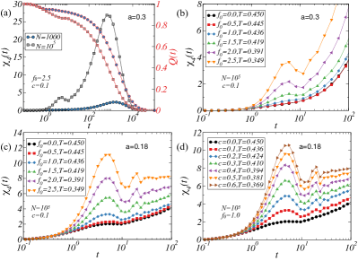
Figure 1: (a). The overlap function $Q(t)$ (black), and its fluctuations $\chi_{4}(t)$ (red) is plotted against time in log scale for two different system sizes. It can be seen that the short time peak in $\chi_{4}(t)$ is more evident for larger system size. (b). This panel highlights the systematic increase in the first peak height, $\chi_{4}^{P1}$, with increasing activity force, $f_{0}$. In panel (a) & (b) analysis is done using the caging parameter $a=0.3$ in the Heaviside function. (c). The panel shows the same plots as (b) but with $a=0.18$, chosen to increase the peak signal even for smaller system sizes and smaller activities. (d). Similar analysis is done with changing $c$, while keeping active force $f_{0}=1.0$, constant. Note that, the temperature is chosen to keep the $\tau_{\alpha}$ same for different activities. Also, this analysis is done on the subsystem with the linear length of $L/3$, where $L$ is the system length, to include the missing fluctuations and better averaging.

On the other hand, the observed strong system size effect in $\chi_{4}^{P1}$ can be used to estimate an underlying intrinsic length scale of the system related to the activity. Tah et al. [49] suggested the equivalence of the dynamic length scale at various time scales, including at $\tau_{\beta}$. Thus it is tempting to equate the length scale to that of the dynamic heterogeneity length scale, but one should be careful as the evolution of dynamic length scale, $\xi_{d}$ in active glassy systems may not be the same as the equilibrium behaviour. Further studies along that line are needed to draw a firm conclusion. The rest of the paper is organized as follows. First, we will briefly discuss the model and methods, then show the phonon nature of the first peak along with systematic finite-size scaling and Block analysis (described later) to obtain the underlying length scale. This paper will end by discussing the role of effective activity parameters and their possible importance to future researches on active glasses.

II Models and methods

In this work, in order to perform the finite-size scaling (FSS), we carry out molecular dynamics simulations over a range of system sizes ($N=400-100000$) of a binary glass-forming liquid in three dimensions (3d), well known in the literature by the name of Kob-Anderson model [50]. In the rest of the paper, it will be referred to as the 3dKA model. The model consists of larger (A-type) and smaller (B-type) particles in the ratio of $80:20$, and we randomly choose the ‘$c$’ fraction of particles as active particles. We varied $c$ in the range $[0-0.6]$. To introduce the activity in the system, we choose the active particles to follow the run and tumble particle (RTP) model with variable active forces $f_{0}$ and fixed persistent time, $\tau_{p}=1.0$ in Lennard Jones units. The concentration of the active particles ($c$) is varied for a fixed $f_{0}$ in order to study the generic nature of the obtained results. It is important to note that the RTP model is crucial for this study. For example, one can use the active Brownian particle (ABP) model, but the most crucial drawback of the ABP model is that it does not include the effect of the inertial term in the equation of motion of the active particles by construction. Our results highlight that the inertial term carries crucial and significant information about the passive as well as the active system. This inertial term is responsible for the collective motion of the particles throughout the system, which is responsible for generating the system’s intrinsic characteristic in terms of long-wavelength phonon-mode.

III Results

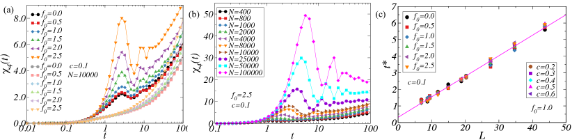
Figure 2: (a)Small time behaviour of $\chi_{4}(t)$ is shown for active-3dKA system of $N=10000$ particles with increasing active force. The light colors represents the cage-relative $\chi_{4}(t)$, while the solid colors are the usual $\chi_{4}(t)$. The enhancement of the first peak with increasing activity can be clearly seen, while its collective nature is confirmed by the absence of the same in the cage relative quantity. (b) System size dependence of the $\chi_{4}(t)$ is shown for the system with active forces $f_{0}=2.5$. The increase in peak height signifies the growth of underlying length scale. (c) The peak position ($t^{*}$) as a function of the system size ($L$) is plotted. The variation turn out to be linear ($t^{*}\sim L$), implying again the phonon nature of the fluctuation.

The relaxation process in supercooled liquids is hallmarked with a small-time plateau in the overlap correlation function $Q(t)$ (see SI for definition), signifying the caging regime. $Q(t)$ indicates the fraction of particles still within their caging distance from the initial time. The caging distance can be parametrized by ‘$a$’. In this study, we choose the temperatures for different values of $f_{0}$ and $c$ such that the structural relaxation time $\tau_{\alpha}$ remains the same as shown in SI. $\tau_{\alpha}$ is defined as $Q(t=\tau_{\alpha})=1/e$. Fig.1(a) contains the $Q(t)$ and $\chi_{4}(t)$ plots for active systems with different system sizes. This analysis of $Q(t)$ and $\chi_{4}(t)$ is done using the Heaviside function with parameter $a=0.3$, the usual value used for the 3dKA model. On increasing the system size, one observes that the peak at early $\beta$-regime emerges and has a systematic trend with activity (see Fig.1(b) for $N=10^{5}$). Note that the time at which the peak appears is linked to the long-range vibrational motion and hence depends on system size in a well-defined manner, as discussed in the subsequent paragraph. To further enhance the signal, we choose the parameter $a=0.18$ in the rest of our analysis (see SI for details). Fig.1(c) shows the monotonic increase in the first peak height of $\chi_{4}^{P1}(t^{*})$ for $N=10^{5}$. Also, the systematic increase in the peak height with increasing the concentration of the active particles (Fig.1(d)) again suggests the peak height maybe directly related to the degree of activity in the system and probably not related to the microscopic origin of the activity. Thus there exists a one-to-one relationship between the amount of activity in the system and the first peak height. This is indeed nice because $\chi_{4}^{P1}$ can be a direct measure of the amount of activity in the system. Next, we discuss the phononic nature of the first peak of $\chi_{4}(t)$ and the characteristic timescale, $t^{*}$.

The confirmation of the phononic nature of the fluctuations comes from two facts. First, suppose this signal is powered by the collective motion of particles. In that case, one can suppress the signal by calculating the same quantities relative to the nearest neighbour cage [51, 52, 53] (cage relative quantities) (see SI for definitions). In Fig.2 (a), we highlight the small-time peak of $\chi_{4}(t)$ with $a=0.18$ in the bolder colours, while the lighter colours are the cage relative $\chi_{4}(t)$ plots. One can see the absence of the same peak in the cage relative $\chi_{4}(t)$, confirming its origin from the collective motions. Note that subsequent peaks can be explained as coming due to the propagation of the same mode in the system. Now, one may argue that all collective motions need not be phononic in nature, so although this confirms the collective nature of the motion, it does not rule out other possibilities. Thus, we look at the system size dependence of the time when the peak appears ($t^{*}$), as shown in Fig.2(b). One can clearly see that the characteristic time increases with increasing system size. If it is due to a phonon, then one expects the characteristic time to scale linearly with system size according to the dispersion relation of phonon, $\omega=Ck$, where $\omega$ is the phonon frequency, $C$ is the sound speed, and $k$ is the wave vector. Fig.2 (c) shows that indeed $t^{*}\sim L$, where $L$ is the linear dimension of the system. It is interesting to note that although $\chi_{4}^{P1}$ increases with increasing activity, the characteristic time scale does not seem to be dependent on the activity. This suggests that phonon mode’s amplitude gets enhanced with increasing activity without much change in the phonon frequency. This fact surely warrants further investigations.

Figure 3: (a). $\chi_{4}^{P1}$ is calculated and plotted against different system sizes, for various active forces to perform the finite size scaling. The calculation is done on subsystem with linear length of $L/4$ to include the missing fluctuations and to obtain better better averaging. (b). The peak height $\chi_{4}^{P1}$, is calculated for and plotted against the block lengths for different activities. The block analysis is performed for $N=10^{5}$ system. (c). The quantity $(g^{uu}-g^{r})/g^{r}(r,\Delta t)$ is plotted as a function of spatial distance for $\Delta t=t^{*}$, here $g^{uu}(r,\Delta t)$ is the displacement-displacement correlation function (Eq.1), and $g^{r}$ is the pair correlation function. The plotted quantity would exponentially decays to zero providing us the correlation length $\xi_{uu}$, which can be clearly seen increasing with increasing activity. The length scale variation with increasing activity can be obtained as a integrated area of the plots and is shown in panel (f). The obtained values are rescaled according to exponential fitted value for $f_{0}=0.0$ to obtain $\xi_{uu}$ (see SI for details). (d). & (e). These panels show the scaling collapse done using scaling ansatz Eq.2 by using the length scales obtained from panel (f).

The next question that comes naturally is the similarity of the signal with the two-dimensional systems. Because of the Mermin-Wagner theorem [54], such fluctuations grow immensely with the increasing system size and diverge in the infinite limit [55]. To explore the same, we took up the finite size analysis (FSS) of the active system. Fig.3(a) shows the system size dependence of $\chi_{4}^{P1}$ calculated and averaged over each quarter of the system length ($L_{4}$). The quarter of the system length is used to increase the averaging and include many important missing fluctuations like fluctuation in density, temperature, concentration of the active particles, etc. [56]. This method of finite size scaling analysis is known as ‘block analysis’ and henceforth we will use the same name in the rest of the article. The plot shows that the peak height increases rapidly with increased system size and would saturate for a large enough system size in contrast to 2D systems. Also, the increase in the peak value becomes more and more drastic with increasing activity. In Ref.[44] it has been shown that the dynamic correlation grows spatially with increasing activity. Our observation of finite size effects on the phonon peak also suggests the growth of some inherent dynamic length scale with increasing activity. Note that in Ref.[49] it has been shown that the dynamic correlation length remains the same at various time scales, including the early $\beta$-regime. Thus it will be important to compute the dynamic length scale at the time scale of phonon peak in an independent manner to see whether the observed finite-size effects in $\chi_{4}^{P1}$ can be rationalized using that length scale. To do so, we turn to compute the displacement-displacement correlation function at $t^{*}$ i.e. $g^{uu}(r,t^{*})$ [49, 57]. It is defined as,

$$g^{uu}(r,\Delta t)=\frac{\left\langle\sum\limits_{i,j=1,j\neq i}^{N}u_{i}(0,\Delta t)u_{j}(0,\Delta t)\delta(r-|\textbf{r}_{ij}(0)|)\right\rangle}{4\pi r^{2}\Delta rN\rho\langle u(\Delta t)\rangle^{2}}$$ (1)

where, $u_{i}(t,\Delta t)=|\textbf{r}_{i}(t+\Delta t)-\textbf{r}_{i}(t)|$, and $\langle u^{2}(\Delta t)\rangle=\langle\frac{1}{N}\sum_{i=1}^{N}\textbf{u}_{i}(t,\Delta t).\textbf{u}_{i}(t,\Delta t)\rangle$. $g^{uu}(r,\Delta t)$ is calculated at time $\Delta t=t^{*}$, along with the usual pair correlation function $g^{r}$. The quantity $g^{uu}(r,\Delta t)/g^{r}-1.0$ would decay to zero as a function of $r$, providing the decorrelation length of particle’s displacement over the time interval $\Delta t$. If one assumes the decay to be exponential, then the area under the curve would provide us with the correlation length without involving any fitting procedure. Fig.3(e) contains the semi-log plot of $g^{uu}(r,\Delta t)/g^{r}-1.0$ calculated for system size of $N=10^{5}$. The observed near linear behaviour confirms the exponential decay. The obtained length scale ($\xi_{uu}$) with increasing activity in the system is plotted in Fig.3(f). The values in the plot are the integrated areas scaled with the absolute value of the length scale obtained by fitting an exponential function to the data for the passive case, $f_{0}=0.0$. Note that the length scale grows by a factor of $\sim 5.5$, while the structural relaxation times remain similar. We then performed the FSS of the data presented in Fig.3(a) using the same length scale using the following scaling ansatz

$$\chi_{4}^{P1}(L,\Omega)=\chi_{4}^{P1}(L\to\infty,\Omega)\mathcal{G}\left[\frac{L}{\xi_{uu}(\Omega)}\right],$$ (2)

where, $\chi_{4}^{P1}(L\to\infty,\Omega)$ is the large system size asymptotic value of the susceptibility peak and $\Omega=cf_{0}^{2}\tau_{p}$ is the effective activity in the system as suggested in Ref.[58].

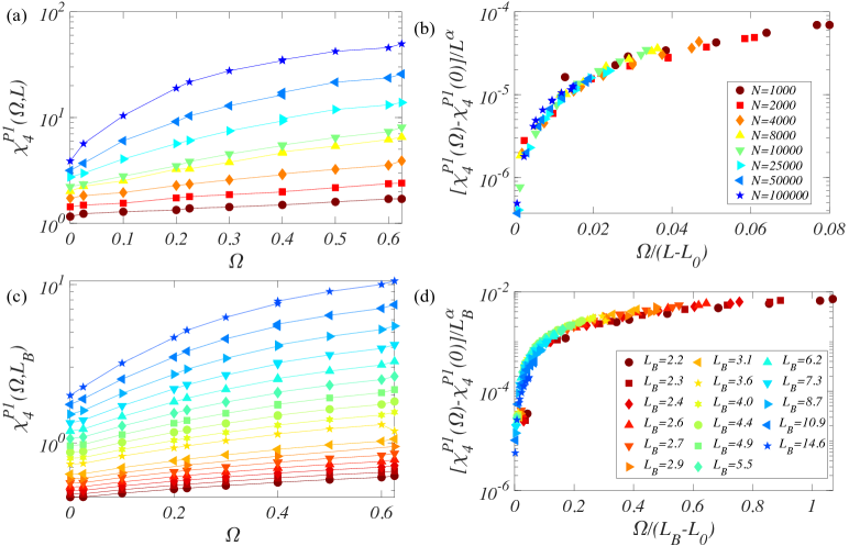
Figure 4: (a) The peak height, $\chi_{4}^{P1}$ is plotted against the effective activity parameter $\Omega=cf_{0}^{2}\tau_{p}$ for different system sizes and different block lengths (c). The singular function while changing the $c$ and $f_{0}$ in $\Omega$ for a particular system size or block length suggests the one-to-one correspondence of $\chi_{4}(PI)$ and net activity in the system. The scaling anstaz Eq.3 is used with the parameters, $L_{0}=1.6$, and $\alpha=4.0$ to collapse both the finite size data and block analysis data in panels (b) and (d) respectively.

The data collapse using Eq.2 observed in Fig.3(b) is indeed very good, suggesting that the length scale can explain the observed finite size effect elegantly. Next, we performed block analysis of the peak height $\chi_{4}(L_{B},f0,t=t^{*})$ computed for varying block size, $L_{B}$ as shown in Fig.3(c), to reconfirm the connection of the peak and underlying dynamic correlation. To our expectation, the block length ($L_{B}$) variation of $\chi_{4}^{P1}$ can be collapsed by assuming the same length scale $\xi_{uu}(\Omega)$ as shown in Fig.3(d). The details of the block analysis are given in the SI. Note that in the top panel of Fig.3, we have shown data with different $f_{0}$ and not included the data with different $c$ for better clarity. While in the bottom panel, all of the variations in terms of effective activity $\Omega$ (also discussed later in the text) are included. Note that $\chi_{4}^{P1}$ depends on the caging parameter $a$, which we have chosen to be $a=0.18$, while the scale obtained from the displacement-displacement correlation function does not depend on such parameters. So one can conclude that the correlated dynamics extend further into the space with increasing activity even at the vibrational time scales, and the increasing peak height signifies the enhancement of phonon amplitude. Thus, $\chi_{4}^{P1}$ indeed seems to be a good and direct measure of both the activity in the system and the correlated dynamic length scale.

Activity in the biological or model systems can be present in various forms. We also tried to reciprocate the same in our system in the following three ways: by changing the concentration of active particles, $c$, or by changing the magnitude of the force on those particles, $f_{0}$, or by increasing the persistence time of active particles, $\tau_{p}$. In Ref.[58], the variable $\Omega=cf_{0}^{2}\tau_{p}$ was used to quantify net activity in the system, and it was shown that within a range of parameter values, this parameter uniquely defines the degree of activity in the system. This means that if one changes $f_{0}$, $c$, and $\tau_{p}$, keeping $\Omega$ the same, one would expect the system’s dynamical behaviour to be the same. It would be interesting to check if $\chi_{4}^{P1}$ also follows this behaviour with changes in the parameters across system sizes. Fig. 4(a) shows the plot of $\chi_{4}^{P1}$ with respect to $\Omega$, and one can see that for both the change in concentration, $c$, and the change in the active force, $f_{0}$, the $\chi_{4}^{P1}$ follows a universal function for given system size. The dependence of $\chi_{4}^{P1}$ on $\Omega$ has strong system size effects. To understand the same in a unified manner, we develop a scaling theory as follows: For a given system size with linear dimension, $L$, the $\chi_{4}^{P1}$ seems to show a saturation tendency above a certain activity, $\Omega=\Omega^{*}(L)$. It is also evident from the data that $\Omega^{*}(L)$ seems to increase with increasing systems size. We proposed the following scaling function to rationalize the observation,

$$\chi_{4}^{P1}(\Omega,L)=L^{\alpha}\mathcal{F}\left(\frac{\Omega}{\Omega^{*}}\right)+\chi_{4}^{P1}(0,L).$$ (3)

Note that at $\Omega=0$, $\chi_{4}^{P1}$ has a finite value that depends on the system size, so we subtract out the part of the contribution in $\chi_{4}^{P1}$, which does not come due to activity. Now, if one takes into account that there is a growing correlation in the system due to activity, then at certain activity $\Omega=\Omega^{*}$ , the correlation length $\xi_{uu}(\Omega^{*})$ will be similar to the length of the simulation box, $L$. If one then increases $\Omega$ further, the correlation length will then be bounded by the finite size of the simulation box. The corresponding susceptibility will also saturate to a value solely controlled by the system size. If one now assumes a dynamical scaling behaviour similar to critical phenomena, then one can expect $\chi_{4}^{P1}(\Omega\to\infty,L)\sim L^{\alpha}$, $\alpha$ being one of the scaling exponents. Now, on the other hand, $\Omega^{*}$ can be obtained by demanding $\xi_{uu}(\Omega^{*})\sim\zeta L$, where $\zeta$ is a scale factor of order unity. Note that $\xi_{uu}(\Omega)$ shows a linear dependence with $\Omega$, as shown in Fig.3 (f). If we assume $\xi_{uu}(\Omega)=\xi_{uu}(0)+A\Omega$, then $\Omega^{*}\sim L-L_{0}$ up to an overall scale factor, where $L_{0}$ is a scaling parameter that depends on the correlation length at $\Omega=0$. Suppose these scaling arguments indeed capture the underlying physics. In that case, one expects that all data shown in Fig.4(a) will fall on a master curve if $[\chi_{4}^{P1}(\Omega,L)-\chi_{4}^{P1}(0,L)]/L^{\alpha}$ is plotted as a function of scaled frequency $\Omega/(L-L_{0})$ with an appropriate choice of the parameter $\alpha$ and $L_{0}$. The validity of this assumption is shown in Fig.4(b). The data collapse with $\alpha=4$ and $L_{0}=1.6$ looks reasonable, suggesting that a scaling theory can describe both activity dependence and system size dependence of $\chi_{4}^{P1}$ in a unified manner.

This also gives us the possibility to quantify the changes in the degree of activity in the system compared to its zero activity value by computing the first peak in four-point susceptibility. It will surely have advantages in experiments in which often estimating the degree of activity is not easy because activity often arises from the internal activity of the constituent particles that cannot be directly controlled in a precise manner by external means. In particular, in experiments involving imaging techniques, often a small part of the whole system is looked at. In that context, it will be essential to check the validity of the same scaling theory if one studies the variation of $\chi_{4}^{P1}$ using the block analysis method. In Fig.4(c) & (d), we did the same analysis for $\chi_{4}^{P1}$ computed for block sizes ($L_{B}$) at various activities ($\Omega$), and the scaling collapse is obtained using the same parameters as used before. The data collapse was again observed to be good. This gives us the confidence that this method will be very useful in experiments.

IV Conclusions

To conclude, we have shown that with increased activity, the fluctuations in the relaxation process in the $\beta$-relaxation regime increase systematically, which was then shown to be linked with the cooperative motion of the particles. This leads to an important inference that one can obtain the amount of activity in the system by looking at its vibrational relaxation process and the associated four-point dynamic susceptibility, $\chi_{4}(t)$. This in the future might play an essential role in determining the degree of activity in experimental systems where the source of active driving can come from the internal processes of the constituent particles and direct control and estimation of the total activity in the system might not be immediately available. In particular, there are experimental studies that measured the $\chi_{4}(t)$ in systems like epithelial monolayers [27], cell assemblies [34]. With the proposed method, one will be able to obtain valuable information about the net activity in the system and a growing dynamical correlation length even by studying the short time dynamics which requires shorter data accusation. This we hope will surely encourage many future experiments both in biological systems as well as synthetic active matter system. Finally, we provided a scaling theory to understand the activity dependence as well as the system size dependence of four-point susceptibility in a unified manner. The results clearly show that the peak height of $\chi_{4}(t)$ at a short timescale is probably be a function of the effective activity parameter $\Omega=cf_{0}^{2}\tau_{p}$ at least within the studied system sizes and parameter ranges.