Abstract

On the 17th of August, 2017 came the simultaneous detections of GW170817, a gravitational wave that originated from the coalescence of two neutron stars, along with the gamma-ray burst GRB170817A, and the kilonova counterpart AT2017gfo. Since then, there has been much excitement surrounding the study of neutron star mergers, both observationally, using a variety of tools, and theoretically, with the development of complex models describing the gravitational-wave and electromagnetic signals. In this work, we improve upon our pipeline to infer kilonova properties from observed light-curves by employing a Neural-Network framework that reduces execution time and handles much larger simulation sets than previously possible. In particular, we use the radiative transfer code POSSIS to construct 5-dimensional kilonova grids where we employ different functional forms for the angular dependency for the dynamical ejecta component. We find that incorporating an angular dependence improves the fit to the AT2017gfo light-curves by up to $\sim$50% when quantified in terms of the weighted Mean Square Error.

1 1 0 https://doi.org/ Using Neural Networks to Perform Rapid High-Dimensional Kilonova Parameter Inference Using Neural Networks to Perform Rapid High-Dimensional Kilonova Parameter Inference Mouza Almualla ^1,†,∗, Yuhong Ning ^2,‡, Pouyan Salehi³, Mattia Bulla^4,5,6,7, Tim Dietrich^3,8, Michael W. Coughlin⁹ and Nidhal Guessoum ¹ Mouza Almualla, Yuhong Ning, Pouyan Salehi, Mattia Bulla, Tim Dietrich, Michael Coughlin and Nidhal Guessoum Almualla, M.; Ning, Y.; Salehi, P.; Bulla, M.; Dietrich, T; Coughlin, M; Guessoum, N Correspondence: mouza.almualla@cfa.harvard.edu Current address: Center for Astrophysics $|$ Harvard & Smithsonian, 60 Garden St, Cambridge, MA 02138, USA Current address: Department of Physics, Brown University, Providence, RI 02906, USA

1 Introduction

The driving idea of multi-messenger astronomy is that a single event observed through different messengers improves our understanding of the physical processes. This concept has gotten additional momentum through the Binary Neutron Star (BNS) detection GW170817 (Abbott et al, 2017) connected with the observation of electromagnetic radiation from gamma-rays to radio waves (Abbott et al., 2017). This event followed the birth of GW astronomy in 2015 (Abbott, B. P. et al., 2016), brought about with the success of the Advanced Virgo (Acernese et al, 2015) and the Advanced LIGO (Aasi et al, 2015) interferometers in detecting GWs emitted by compact object mergers. In general, BNS and Neutron Star – Black Hole (NSBH) mergers may be accompanied by an optical/infrared counterpart, referred to as a kilonova, which will give us important insights into what is possibly one of the most dominant sites of rapid neutron capture (r-process) elements in the Universe; see Metzger (2017) for a review. Our first and as yet only confirmed discovery of a kilonova from a BNS merger, AT2017gfo in NGC 4993 (D $\sim 40$ Mpc) (Coulter et al., 2017), was achieved through follow-up of GW170817 by multiple telescope facilities around the globe, and is an exceptional demonstration of the potential of multi-messenger astronomy in contributing to scientific knowledge (Abbott et al., 2017). These detections were also accompanied by the discovery of short gamma-ray burst GRB 170817A (Abbott et al., 2017). Through this event, we learned more about the aforementioned r-process nucleosynthesis (e.g., Chornock et al., 2017; Coulter et al., 2017; Cowperthwaite et al., 2017; Pian et al., 2017; Smartt et al., 2017; Watson et al., 2019; Kasliwal et al., 2019) and also placed constraints on the expansion rate of the Universe (Abbott et al., 2017; Guidorzi et al., 2017; Hotokezaka et al., 2019; Coughlin et al., 2020; Dhawan et al., 2020; Dietrich et al., 2020) and the neutron star equation of state (e.g., Bauswein et al., 2017; Margalit and Metzger, 2017; Coughlin et al., 2019a, b; Annala et al., 2018; Most et al., 2018; Radice et al., 2018; Abbott et al., 2018; Lai et al., 2019; Dietrich et al., 2020; Huth et al., 2021).

Inferring kilonova model parameters from observational data requires a thorough understanding of the ejecta composition, behaviour, and morphology (e.g., Dietrich et al., 2020; Nedora et al., 2022; Nicholl et al., 2021; Breschi et al., 2021); in addition, there are various parts of the parameter inference pipeline that must be improved upon and optimized such that we are able to efficiently utilize the available data and learn more about the progenitors. Radiative transfer simulations have been most commonly used to generate expected supernova and kilonova light-curves, (e.g., Tanaka, 2016; Kasen et al., 2017; Wollaeger et al., 2018; Bulla, 2019; Kawaguchi et al., 2020).

There are two major sources of ejecta from the progenitor system. The first is known as the dynamical ejecta, ejected ‘dynamically’ around the moment of merger through torque or shocks (at merger or in the early-postmerger phase) (e.g., Metzger et al., 2008; Bauswein et al., 2013). The second source of ejecta comes from the post-merger wind, i.e., outflows from an accretion disk formed around the central remnant, consisting of the unbound debris resulting from the merger (e.g., Siegel and Metzger, 2018; Metzger, 2019). The dynamical source is ejected on a timescale of milliseconds, while the latter is formed on a timescale of up to seconds.

There are two major dynamical ejection processes in BNS mergers. The first is through shocks that forms at the contact interface of the merging stars or at core bounces in the early postmerger phase (Hotokezaka and Piran, 2015). The second component is the tidal ejecta, and is due to tidal interactions that arise from the non-axisymmetric gravitational forces at play in the binary system (Hotokezaka and Piran, 2015; Metzger, 2019). Recent simulations (Radice et al., 2018; Nedora et al., 2022) show that the more neutron-rich, lower $Y_{e}$ ejecta ($Y_{e}\lesssim 0.1$) arises from the aforementioned tidal component, and is located closer to the equatorial plane, while the ejecta arising from the shock component tends to have a relatively higher electron fraction (going up to $Y_{e}\sim\,0.4$) and is approximately isotropic.

The disk mass is $\sim 0.01-0.3M_{\odot}$ (Oechslin and Janka, 2006), and is usually much lower when the remnant immediately collapses into a black hole; this is due to the lack of time for the remnant to redistribute its angular momentum and mass as it transforms from a differentially rotating to a solid rotating body, thus preventing the formation of a more massive disk (Metzger, 2019). A fraction of the disk is ejected in the form of a post-merger disk wind, with the exact value being uncertain and ranging from 20 to 40 per cent (e.g. Just et al., 2015; Siegel and Metzger, 2018; Miller et al., 2019; Fernández et al., 2019; Fujibayashi et al., 2020). The post-merger wind usually dominates the dynamical ejecta (Wu et al., 2016). Works such as Fernández and Metzger (2013) show the disk wind ejecta $Y_{e}$ ranging within $\sim 0.2-0.4$ when the remnant collapses into a black hole. The electron fractions present in the case of both dynamical and post merger wind cases are suitable for the production of heavy r-process elements (Rosswog et al., 2014).

With the gravitational-wave detector networks’ fourth observing run nearing, one needs to continue to improve the instruments and software tools that we use to analyze the forthcoming multi-messenger detections. These mergers bring rich knowledge to various fields of physics and astronomy, from the understanding of such events and the big, powerful jets of relativistic particles that they produce, to the physical structure of both the neutron stars (internally) and the matter that is ejected in the merger, not to mention the detailed characteristics of the gravitational waves that are emitted. Much work is being done on the theoretical front to prepare us for the ‘treasure trove’ of data from upcoming detections. In particular, models of kilonovae are being constructed with increased complexity and fine-tuning (e.g., Korobkin et al., 2021; Zhu et al., 2021; Wollaeger et al., 2021).

In this work, we use POSSIS (Bulla, 2019), a Monte-Carlo radiative transfer code, in order to produce “model grids” that sample the parameter space for any given ejecta morphology. In particular, we use an updated version of POSSIS (Bulla, 2022) including improved heating rates from Rosswog and Korobkin (2022) and wavelength- and time-dependent opacities from Tanaka et al. (2020) that depend on local properties of the ejecta (density, temperature and $Y_{e}$). Details about these new implementations can be found in Bulla (2022). Previous works such as Coughlin et al. (2018); Dietrich et al. (2020); Heinzel et al. (2021) used Gaussian Process Regression (GPR) to interpolate within kilonova grids to perform parameter estimation. Here, we introduce a Neural Network (NN) framework that significantly enhances the speed of the interpolation step and scales well for much larger grids. In addition, due to the importance of understanding the effects of different ejecta morphologies on the computed light-curves, we explore different functional forms for the angular dependence in the density profile of the dynamical ejecta.

Our paper is structured as follows, in Sec. 2, we describe the NN architecture. In Sec. 3, we discuss and evaluate the different density profiles for the dynamical ejecta in the context of GW170817/AT2017gfo. Finally, we summarize our conclusions and outline ways of moving forward in Sec. 4.

2 Methods: A New Surrogate Generation Framework

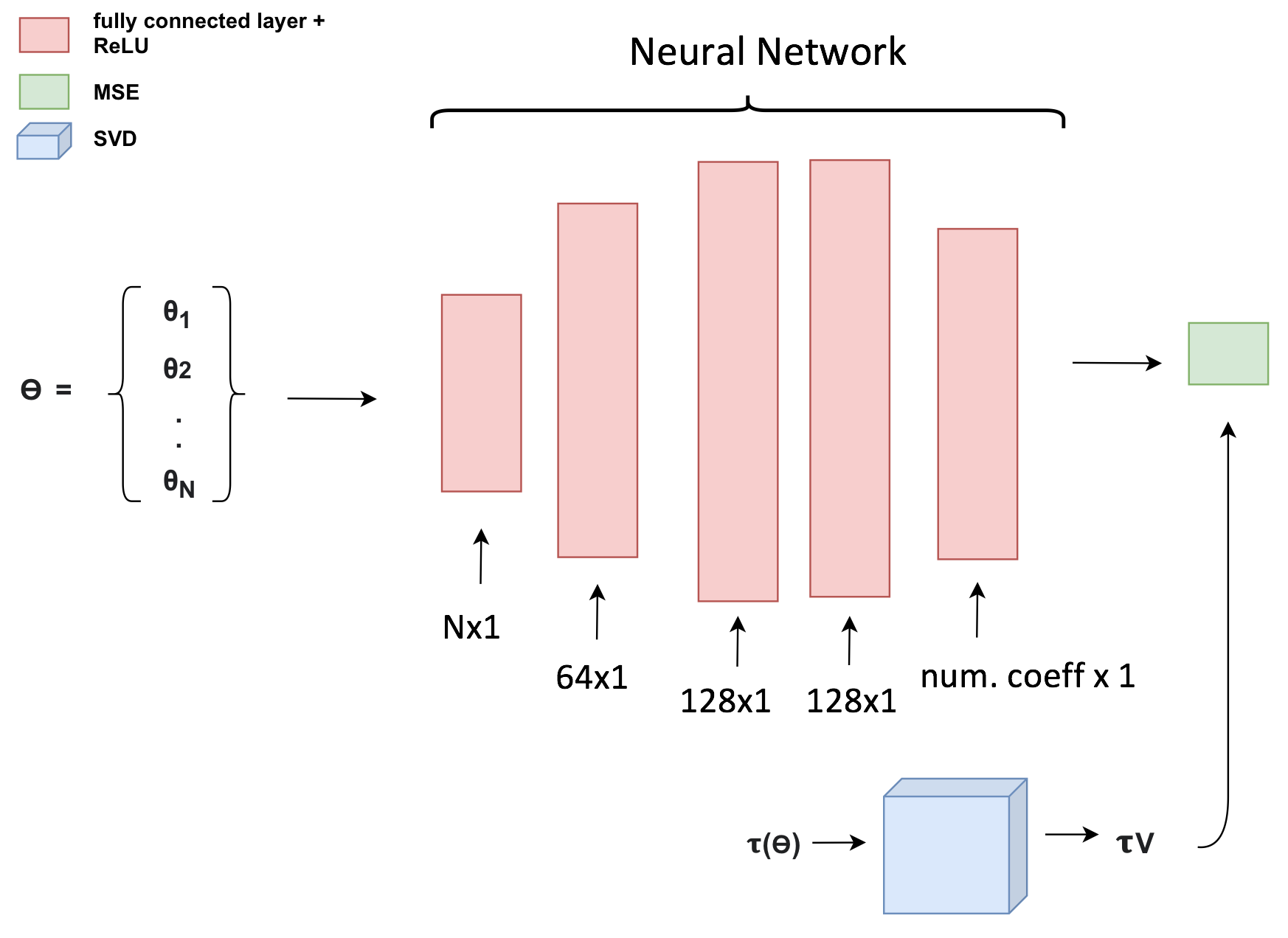
Figure 1: A diagram of the interpolation framework used in this work. The input to our network is the model parameters, and the network is trained on a PCA-like projection of our photometric and bolometric data onto the right-singular vector. Five fully-connected layers are shown, and an MSE loss function is employed.

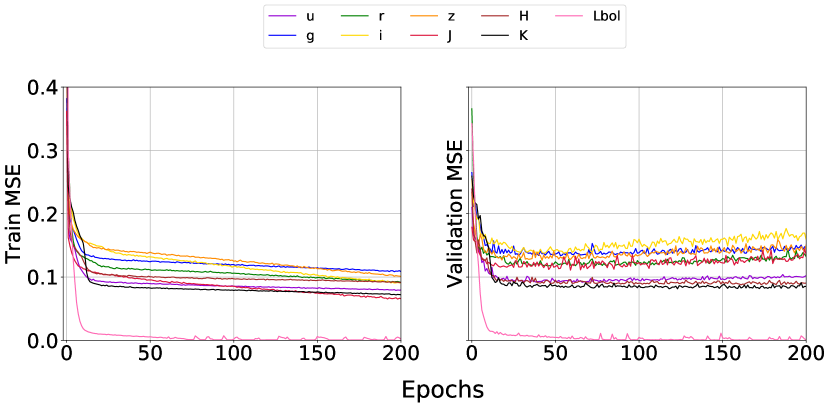
Figure 2: The MSE loss is shown for the $u$, $g$, $r$, $i$, $z$, $y$, $J$, $H$, and $K$ bands, as well as for the bolometric luminosity. The loss for the train set is shown in the left subplot, and for the validation set in the right subplot. After $\sim$ 200 epochs, the network tends to over-fit the train data, so we stop training at this point.

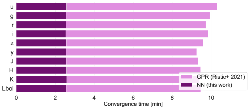
Figure 3: Convergence time for all of the photometric bands used in this work, as well as for the bolometric luminosity. The NN framework is shown in dark purple, while the interpolation scheme from Ristic et al. (2021) is shown in light purple.

2.1 Preprocessing

Instead of directly inputting our bolometric and photometric light-curves into our Neural Network for interpolation, we follow the procedure of Doctor et al. (2017) and Coughlin et al. (2018), using Singular Value Decomposition (SVD) to perform a dimensionality reduction on our data and produce the principle components of our light-curve vectors, i.e., a new basis for our data in which different dimensions of the data are most uncorrelated. We then train our neural network on this output in order to produce a so-called “surrogate model” that interpolates our original model grid. Denoting our photometric and bolometric light-curves as $\tau(\mathbf{\Theta})$, where $\mathbf{\Theta}$ represents the set of parameters for a given model, SVD decomposes $\tau(\mathbf{\Theta})$ as follows:

$$\tau=U\Sigma V^{T}$$ (1)

where $\Sigma$ is a diagonal matrix containing the singular values of $\tau(\mathbf{\Theta})$, and the columns of U and V are orthonormal bases called the left-singular and right-singular vectors, respectively. We can then obtain the principle component analysis (PCA) output by projecting $\tau(\mathbf{\Theta})$ onto the right singular matrix:

$$\tau V=PCA$$ (2)

Note that we first normalized our light curves before performing PCA, and the right singular vector $V$ was truncated to 100 basis vectors. A train/validation split of 90/10 was used.

2.2 Neural Network Architecture

Our NN consists of five ReLU-activated (Rectified Linear Units, i.e., $R(z)=\text{max}(0,z)$ for each neuron) fully-connected layers, as shown in Figure 1, with the first layer containing $N$ weights corresponding to the number of parameters for the model, three hidden layers, and the output layer having a number of weights equal to the number of columns in our PCA output. We used a batch size of 32 and trained for 200 epochs, using a mean-square error (MSE) loss function.

The use of a NN is much more efficient for higher-dimensional kilonova models than GPR, which usually performs poorly when a model has more than four parameters. To demonstrate the performance of our interpolation framework, we use a model (to be described in-depth in the following sections) that has 5 parameters and 1,260 total parameter combinations comprising our simulation set. Training 10 different networks (one for each photometric band $u$, $g$, $r$, $i$, $z$, $y$, $J$, $H$, $K$, and in addition one for the bolometric luminosity) took on the order of $\sim$ 40 mins. The MSE loss is shown as a function of epoch in Figure 2. Our model does not over- or under-fit the train data, since we can see very similar performance on our validation set in the right subplot as compared to the train set. In addition, our network converges very quickly, so even 50 epochs would be sufficient in constructing our surrogate.

We also compare our NN framework to state-of-the-art interpolation methods, such as the GPR framework used in Coughlin et al. (2018); Heinzel et al. (2021), as well as that in Ristic et al. (2021), in terms of its computational efficiency. It took upwards of 13 hours for the former GPR implementation from Coughlin et al. (2018) (which uses the scikit-learn library) to construct our model in the $u$-band, and so we only use the framework from Ristic et al. (2021) in this comparison. The performance for each model is shown in Figure 3. In addition to the benefits in terms of convergence time, the output of the NN interpolation scheme takes up a lot less memory – on the order of tens of MB, in comparison to a few GBs for the scikit-learn GPR scheme. Even more importantly, the total time it takes to perform parameter inference is significantly reduced due to the much simpler loading procedure for NNs; for the 5-dimensional model used here, loading for all of the bands and the bolometric luminosity takes a total of $\sim$700 ms for the NN, while for the GPR approach from Ristic et al. (2021), it takes $\sim$ 80 min (since some components need to be recalculated). This is a significant improvement when considering that the parameter inference takes $\approx$20 min excluding the loading step.

Future work in improving the performance of our model includes incorporating batch normalization, drop out layers, and various other easily implementable techniques. The wealth of developments in deep learning allows for a significant improvement in computational efficiency whilst still maintaining high accuracies and developing surrogate models with high fidelity.

3 Results: Angular Dependencies in the Dynamical Ejecta

Numerical relativity simulations provide valuable information about what we can expect from the ejected matter in the merger of BNSs. As the field develops, these simulations have become more and more complex, incorporating neutrino transport and more realistic neutron star equations of state. We know that there are two primary ejection processes, described in Section 1, but the exact geometry of each of these components are now known; note that also the ejecta opacities are another point of uncertainty in kilonova simulations and we refer to Appendix A for a preliminary exploration of this. Generally, the density profile of the post-merger wind is thought to be relatively spherically symmetric, while the density profile of the dynamical ejecta will have an angular dependence such that the mass is more concentrated in equatorial regions as compared to polar regions (e.g., Dietrich and Ujevic, 2017; Kawaguchi et al., 2020; Nedora et al., 2022).

There are various functional forms that have been used in kilonova modelling to incorporate this angular dependency into the dynamical ejecta. We will explore a few of them, and then use data from AT2017gfo to infer which provides the best fit to the observed light-curves. We remark that in our simulations, we will only consider the case in which the post-merger wind is slower than the dynamical ejecta. We use the so-called Spherical segment-Spherical Cap geometry (shortened as SSCr, with $r$ signifying that re-processing between the different ejecta components is taken into account); see the left-most geometry in Figure 1 of Heinzel et al. (2021). The density profiles for the different ejecta components are represented as follows:

$$\rho(r,t)\propto\begin{cases}r^{-\alpha}t^{-3}&v_{\text{pm,min}}\leq r/t\leq v_{\text{pm,max}}\\ \eta(\theta)r^{-\alpha}t^{-3}&v_{\text{pm,max}}\leq r/t\leq v_{\text{dyn,max}}\end{cases}$$

where we set $\alpha$=3, $v_{\text{pm,min}}=0.025c$, $v_{\text{pm,max}}=0.08c$, $v_{\text{dyn,max}}=0.3c$. $\eta(\theta)$ is the term introducing the angular dependence with respect to $\theta$, the angle measured from the polar axis, into the dynamical ejecta. The forms that we will first explore are:

1) a sinusoidal relationship, i.e., $\eta(\theta)=\sin^{2}(\theta)$, also used by Perego et al. (2017) based on numerical-relativity simulations from Radice et al. (2018); and

2) a function defined in Kawaguchi et al. (2020):

$$\eta(\theta)=(1-\Theta(\theta))f_{\text{d}}+\Theta(\theta)$$ (3)

$$\Theta(\theta)=\frac{1}{1+\exp{[-10(\theta-\pi/4])]}}$$ (4)

where $f_{d}$ determines the strength of the angular dependence from equatorial to polar angles. We will call the latter the “Kawaguchi Model.” As can be seen in Figure 4, with the sinusoidal functions, we have a very gradual increase, whereas with the dependency from Kawaguchi et al. (2020) the density profile will be much more concentrated for $\pi/4\leq\theta\leq 3\pi/4$.

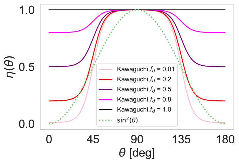
Figure 4: Different functional forms for the angular dependency in the dynamical ejecta. This is shown for $\sin^{2}(\theta)$ and Equations (3) and (4). $\theta$ represents the angle from the polar axis.

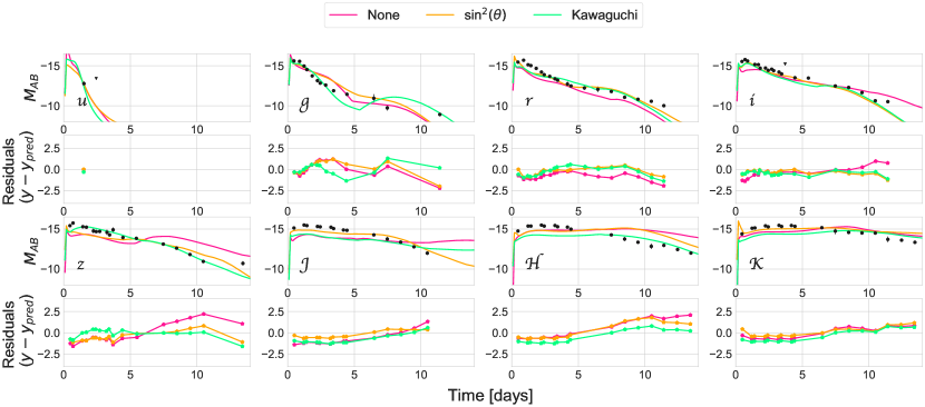
Figure 5: Best-fit light-curves in the $u$, $g$, $r$, $i$, $z$, $J$, $H$, and $K$ bands are plotted for three different models in which the angular dependency in the dynamical ejecta is varied. The AT2017gfo observations are plotted as black dots, the Kawaguchi best-fit is plotted in green, the $\sin^{2}(\theta)$ best-fit is plotted in orange, and the model with no angular dependency is plotted in pink. We also plot the residuals in each band.

For our first analysis here, we will be pinning $f_{d}$ at 0.01 as done in Kawaguchi et al. (2020), since this produces the strongest angular dependency and will be a useful comparison. Our model has the following four free parameters: the dynamical ejecta mass $M_{\text{ej,dyn}}$, post-merger wind ejecta mass $M_{\text{ej,dyn}}$, half-opening angle of the lanthanide-rich component of the dynamical ejecta $\phi$, and the observing angle $\theta_{\text{obs}}$. For the dynamical and post-merger wind ejecta masses, we perform logarithmic sampling across the interval [0.001, 0.1]. Our entire sample set used to generate our model grids is shown in Table 1.

Table 1: The parameters of our model and the sample values for which we run POSSIS.

Parameters	Samples
$M_{\text{ej,dyn}}$/$M_{\odot}$	[0.001, 0.00251, 0.00631, 0.0158, 0.0398, 0.1]
$M_{\text{ej,win}}$/$M_{\odot}$	[0.001, 0.00251, 0.00631, 0.0158, 0.0398, 0.1]
$\phi$ [deg]	[0, 15, 30, 45, 60, 75, 90]
$\cos{(\theta_{\text{obs}})}$	[0, 0.1, 0.2, 0.3, 0.4, 0.5, 0.6, 0.7, 0.8, 0.9, 1.0]

We generate 3 model grids: 1) no angular dependence, 2) angular dependence $\eta=\sin^{2}(\theta)$, and 3) the Kawaguchi model with $f_{d}$=0.01. We thus run POSSIS over the aforementioned parameter space, generating $6\times 6\times 7=252$ simulations for each model, and then used the NN interpolation described in Section 2 to interpolate the grid. We then perform parameter inference and find the maximum likelihood estimates for AT2017gfo using PyMultiNest, which is capable of performing both model selection and parameter inference. Using PyMultiNest, we extract posterior distributions for each of the aforementioned parameters. We assume uniform priors that extend over the limits of the grid in the parameter space. The results of the inference (i.e., the best-fit light-curves), assuming $\pm 1$ mag systematic error, for each of these models are shown in Figure 5.

Inspecting by eye, we can see in Figure 5 that across all bands the $\sin^{2}(\theta)$ and Kawaguchi models result in residuals closer to 0. We can further quantify this by obtaining the MSE for each model. However, since the Local Thermodynamic Equilibrium (LTE) assumption in POSSIS is likely to fail at late times when the ejecta become optically thin, and the brighter early-time emission is more important for observational purposes, it is reasonable to perform a Weighted MSE (WMSE) prioritizing the early observations. We thus use the following equation:

$$\text{WMSE}=\frac{1}{n}\frac{\sum_{i=0}^{n-1}\omega_{i}(M_{\text{obs}}-M_{\text{pred}})^{2}}{\sum_{i=0}^{n-1}\omega_{i}}$$ (5)

where $\omega_{i}=\ln{(|M_{\text{obs}}|+1)}+1$. Having done so, we obtain the WMSE values shown in Table 2, and verify our conclusion that incorporating some form of an angular dependence improves the fit to AT2017gfo across almost all bands.

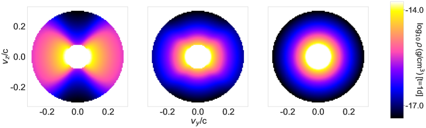
Figure 6: 2D dynamical ejecta density profiles for $f_{d}$=0.01, $f_{d}$=0.5, $f_{d}$=1.0.

The parameter $f_{d}$ allows us also to assess which dependence provides the best fit to the measured light-curves. In Figure 6, we show the 2D density profile for different $f_{d}$’s (0.01, 0.5, 1.0) for comparison.

For this analysis, we include $f_{d}$ as an additional parameter to those listed in Table 1, sampling $f_{d}=[0.01,0.2,0.5,0.8,1.0]$. This increases our simulation set to 1260 simulations. The resulting corner plot of our posteriors is shown in Figure 7. We also include the WMSE values with our maximum-likelihood $f_{d}$ in Table 2.

Table 2: WMSE values for each band and model, for when no angular dependence is incoporated, versus a $\sin^{2}(\theta)$ dependency, versus the Kawaguchi equation when pinning $f_{d}$ at 0.01, and finally when allowing $f_{d}$ to vary (i.e., $f_{d}=0.50$).

Band	Models
	None	$\sin^{2}(\theta)$	$f_{d}=0.01$	best-fit $f_{d}$
$g$	0.0642	0.0571	0.0291	0.0738
$r$	0.0461	0.0127	0.0204	0.0227
$i$	0.0242	0.0119	0.0154	0.0034
$z$	0.0771	0.0313	0.0160	0.0109
$J$	0.0781	0.0164	0.0649	0.0317
$H$	0.0846	0.0593	0.0506	0.0412
$K$	0.0249	0.0168	0.0370	0.0340
average	0.0570	0.0294	0.0333	0.0311

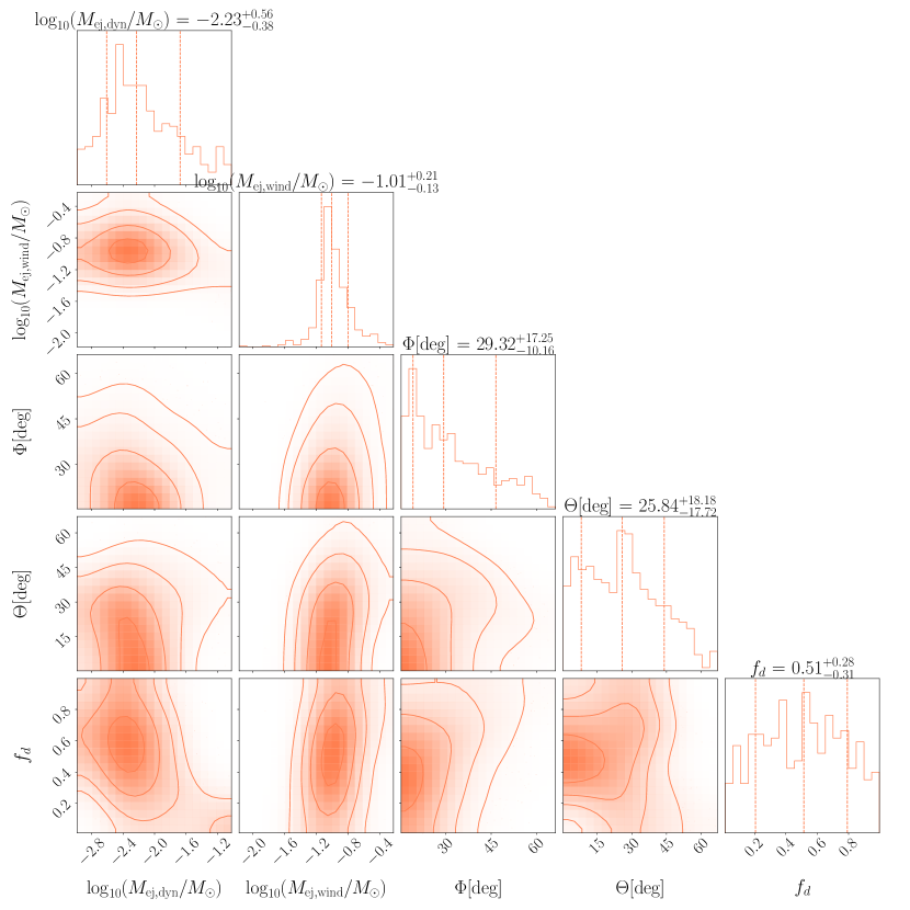
Figure 7: Corner plot showing the resulting posteriors for our model with $f_{d}$ as a free parameter. We can see that all of our inferred parameters are within reasonable ranges and that the distribution for $f_{d}$ is centered around 0.50.

We can see that $f_{d}\sim\,0.50^{+0.28}_{-0.32}$ provides the most optimal fit. When fitting for $f_{d}$, the previous WMSE of 0.0333 decreases to 0.0311. The fit is significantly better in redder bands with $f_{d}$=0.50, while it would be better using a stronger dependency $f_{d}=0.01$ with respect to bluer $g$ and $r$ bands. In order to confirm this behavior, we also run the inference with an assumed systematic error of 0.5 mag (instead of 1.0), and find that the distribution is even more clearly distributed around $f_{d}\sim 0.6$, and the WMSE further decreases to 0.0252. A moderate angular dependence is thus preferred.

Table 3: Resultant posteriors for $M_{\text{ej,pm}}$, $M_{\text{ej,dyn}}$, $\phi$, and $\theta_{\text{obs}}$ for each of the models explored in this section. Uncertainties are shown at the 15th and 85th percentiles.

Model	Parameters
$\eta(\theta)$	$M_{\text{ej,dyn}}$ [$\times 10^{-3}M_{\odot}$]	$M_{\text{ej,pm}}$ [$M_{\odot}$]	$\phi$ [deg]	$\theta_{\text{obs}}$ [deg]
$1$	$4.57_{-2.48}^{+21.88}$	$0.110_{-0.0302}^{+0.0488}$	$44.29_{-13.69}^{+11.85}$	$32.01_{-19.00}^{+19.38}$
$\sin^{2}(\theta)$	$3.09_{-1.51}^{+18.29}$	$0.0912_{-0.032}^{+0.209}$	$36.03_{-12.77}^{+14.04}$	$24.86_{-17.43}^{+24.89}$
kawaguchi ($f_{d}=0.01$)	$19.05_{-11.98}^{+35.90}$	$0.0832_{-0.0405}^{+0.0456}$	$26.95_{-8.03}^{+12.28}$	$37.87_{-19.50}^{+15.77}$
kawaguchi (varied $f_{d}$)	$5.89_{-3.43}^{+15.49}$	$0.0977_{-0.0236}^{+0.0645}$	$29.32_{-10.16}^{+17.25}$	$25.84_{-17.72}^{+18.18}$

To finalize our exploration of different angular dependencies, we summarize the inferred constraints on $M_{\text{ej,pm}}$, $M_{\text{ej,dyn}}$, $\phi$, and $\theta_{\text{obs}}$ for each model in Table 3.

4 Conclusions

In this work, we have modified and improved upon the present parameter inference pipeline used to infer ejecta parameters from observed kilonova light-curves (Coughlin et al., 2018; Dietrich et al., 2020). We constructed an NN framework that sufficiently models the sampled lightcurves and produces a surrogate model with a much improved computational efficiency as compared to previous surrogate construction methods.

We explored the possible nature of AT2071gfo’s ejecta geometry. Specifically, we looked at the angular dependence in the density profile of the dynamical ejecta, showing that some form of angular dependence is beneficial and provides better fits to GW710817/AT2017gfo, with the $\sin^{2}(\theta)$ and the Kawaguchi functional forms both outperforming the model with no angular dependence. The $\sin^{2}(\theta)$ dependence improves the fit across all bands by $\sim$50%.

When using the Kawaguchi equation – parameterized by $f_{d}$, which is approximately the ratio of the density in the polar region ($0\leq\theta\leq\pi/4$) to that in the equatorial region ($\pi/4\leq\theta\leq\pi/2$) – to study the angular dependence, we found that $f_{d}\sim 0.50$ is most suitable. Fitting for $f_{d}$ especially improves performance in the redder bands, decreasing the WMSE by 34% when considering lightcurves in the $i$-band and onwards.

Although we explored one specific aspect of the ejecta structure in this work, and there have been other recent explorations of different kilonova ejecta morphologies (Darbha and Kasen, 2020; Heinzel et al., 2021; Korobkin et al., 2021), there is still much to explore. There are countless other geometries that could be considered for the kilonova ejecta, so an interesting path forward would be performing inference on a “super-geometry” that samples a much wider range of possible ejecta morphologies.

Conceptualization, M.A., Y.N., M.B., T.D.; methodology, M.A., Y.N.; software, M.B., Y.N., M.A.; validation, Y.N., M.B.; formal analysis, M.A., T.D., M.C., N.G.; investigation, M.A.; resources, M.B.; data curation, M.A.; writing—original draft preparation, M.A.; writing—review and editing, Y.N., M.B., T.D., M.C., N.G.; visualization, M.A.; supervision, M.B., T.D., M.C., N.G.; project administration, M.B., T.D., M.C., N.G.; funding acquisition, M.B., T.D., M.C. All authors have read and agreed to the published version of the manuscript.

M.B. acknowledges support from the Swedish Research Council (Reg. no. 2020-03330) and from the European Union’s Horizon 2020 Programme under the AHEAD2020 project (grant agreement n. 871158). M.W.C. acknowledges support from the National Science Foundation with grant Nos. PHY-2010970 and OAC-2117997. T.D. acknowledges financial support through the Max Planck Society.

The data presented in this study are openly available at https://github.com/mbulla/kilonova_models.

Appendix A Introducing an Opacity-Scaling Parameter

Our simulations use state-of-the-art opacities for r-process elements (Tanaka et al., 2020). However, uncertainties in the opacities are likely to be present due to the challenges in modelling the myriad of line transitions expected for these heavy elements.

Given these inherent uncertainties, we introduce the free parameter $\alpha_{\kappa}$ that scales the opacities, and in turn, fine-tunes the emitted flux and color of the kilonova. We assume, for simplicity, that the relative uncertainties are constant across time and wavelength, although this is likely to be more complicated in reality.

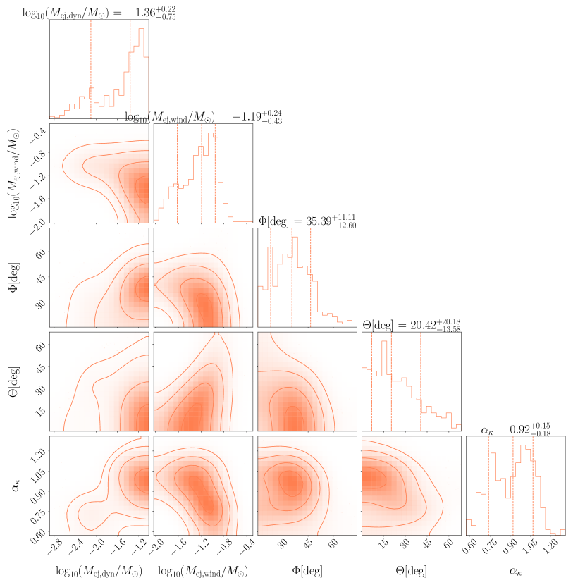
Figure 8: Posteriors showing that $\alpha_{\kappa}$ has a bimodal distribution when fit to GW170817/AT2017gfo lightcurves and a $\sin^{2}(\theta)$ dependency is assumed.

In exploring this, we use the $\sin^{2}(\theta)$ model, given its good performance in Section 3. We use the same sample set as in Table 1, including our new parameter $\alpha_{\kappa}$=[0.75,1.0,1.25]. The resulting corner plot is shown in Figure 8, and we can clearly see a bimodal distribution, with one peak centered at $\alpha_{\kappa}\sim$ 1.04, and one centered at $\sim$ 0.75.

Hence, while at first glance it seems that introducing an opacity rescaling might improve the performance of the model, more work is required for a reliable estimation of the opacities. In particular, the strong bimodal nature of the distribution indicates that a simple time-independent rescaling of the opacities, as employed in this work, might not be applicable. And so, further work exploring either the temporal or the wavelength dependence of the ejecta opacities would be interesting, and may serve to limit the associated systematic errors.

References

References

- Abbott et al (2017) Abbott et al. GW170817: Observation of Gravitational Waves from a Binary Neutron Star Inspiral. Phys. Rev. Lett. 2017, 119, 161101. https://doi.org/10.1103/PhysRevLett.119.161101.
- Abbott et al. (2017) Abbott et al.. Multi-messenger Observations of a Binary Neutron Star Merger. Astrophysical Journal Letters 2017, 848, L12. https://doi.org/10.3847/2041-8213/aa91c9.
- Abbott, B. P. et al. (2016) Abbott, B. P. et al.. Observation of Gravitational Waves from a Binary Black Hole Merger. Phys. Rev. Lett. 2016, 116, 061102. https://doi.org/10.1103/PhysRevLett.116.061102.
- Acernese et al (2015) Acernese et al. Advanced Virgo. Classical and Quantum Gravity 2015, 32, 024001.
- Aasi et al (2015) Aasi et al. Advanced LIGO. Classical and Quantum Gravity 2015, 32, 074001.
- Metzger (2017) Metzger, B.D. Kilonovae. Living Rev. Rel. 2017, 20, 3, [arXiv:astro-ph.HE/1610.09381]. https://doi.org/10.1007/s41114-017-0006-z.
- Coulter et al. (2017) Coulter, D.A.; Foley, R.J.; Kilpatrick, C.D.; Drout, M.R.; Piro, A.L.; Shappee, B.J.; Siebert, M.R.; Simon, J.D.; Ulloa, N.; Kasen, D.; et al. Swope Supernova Survey 2017a (SSS17a), the optical counterpart to a gravitational wave source. Science 2017, 358, 1556–1558, [arXiv:astro-ph.HE/1710.05452]. https://doi.org/10.1126/science.aap9811.
- Abbott et al. (2017) Abbott et al.. Gravitational Waves and Gamma-Rays from a Binary Neutron Star Merger: GW170817 and GRB 170817A. The Astrophysical Journal Letters 2017, 848, L13.
- Chornock et al. (2017) Chornock et al.. The Electromagnetic Counterpart of the Binary Neutron Star Merger LIGO/Virgo GW170817. IV. Detection of Near-infrared Signatures of r -process Nucleosynthesis with Gemini-South. The Astrophysical Journal Letters 2017, 848, L19.
- Cowperthwaite et al. (2017) Cowperthwaite, P.S.; Berger, E.; Villar, V.A.; et al. The Electromagnetic Counterpart of the Binary Neutron Star Merger LIGO/Virgo GW170817. II. UV, Optical, and Near-infrared Light Curves and Comparison to Kilonova Models. The Astrophysical Journal Letters 2017, 848, L17, [arXiv:astro-ph.HE/1710.05840]. https://doi.org/10.3847/2041-8213/aa8fc7.
- Pian et al. (2017) Pian et al.. Spectroscopic identification of r-process nucleosynthesis in a double neutron-star merger. Nature 2017, 551, 67 EP –.
- Smartt et al. (2017) Smartt et al.. A kilonova as the electromagnetic counterpart to a gravitational-wave source. Nature 2017, 551, 75 EP –.
- Watson et al. (2019) Watson, D.; Hansen, C.J.; Selsing, J.; Koch, A.; Malesani, D.B.; Andersen, A.C.; Fynbo, J.P.U.; Arcones, A.; Bauswein, A.; Covino, S.; et al. Identification of strontium in the merger of two neutron stars. Nature 2019, 574, 497–500. https://doi.org/10.1038/s41586-019-1676-3.
- Kasliwal et al. (2019) Kasliwal, M.M.; Kasen, D.; Lau, R.M.; Perley, D.A.; Rosswog, S.; Ofek, E.O.; Hotokezaka, K.; Chary, R.R.; Sollerman, J.; Goobar, A.; et al. Spitzer Mid-Infrared Detections of Neutron Star Merger GW170817 Suggests Synthesis of the Heaviest Elements. Monthly Notices of the Royal Astronomical Society: Letters 2019, [http://oup.prod.sis.lan/mnrasl/advance-article-pdf/doi/10.1093/mnrasl/slz007/27503647/slz007.pdf]. https://doi.org/10.1093/mnrasl/slz007.
- Abbott et al. (2017) Abbott, B.P.; Abbott, R.; Abbott, T.D.; Acernese, F.; Ackley, K.; Adams, C.; Adams, T.; Addesso, P.; Adhikari, R.X.; Adya, V.B.; et al. A gravitational-wave standard siren measurement of the Hubble constant. Nature 2017, 551, 85–88, [1710.05835]. https://doi.org/10.1038/nature24471.
- Guidorzi et al. (2017) Guidorzi, C.; et al. Improved Constraints on from a Combined Analysis of Gravitational-wave and Electromagnetic Emission from GW170817. Astrophys. J. Lett. 2017, 851, L36, [arXiv:astro-ph.CO/1710.06426]. https://doi.org/10.3847/2041-8213/aaa009.
- Hotokezaka et al. (2019) Hotokezaka, K.; Nakar, E.; Gottlieb, O.; Nissanke, S.; Masuda, K.; Hallinan, G.; Mooley, K.P.; Deller, A.T. A Hubble constant measurement from superluminal motion of the jet in GW170817. Nature Astronomy 2019. https://doi.org/10.1038/s41550-019-0820-1.
- Coughlin et al. (2020) Coughlin, M.W.; Dietrich, T.; Heinzel, J.; Khetan, N.; Antier, S.; Bulla, M.; Christensen, N.; Coulter, D.A.; Foley, R.J. Standardizing kilonovae and their use as standard candles to measure the Hubble constant. Physical Review Research 2020, 2. https://doi.org/10.1103/physrevresearch.2.022006.
- Dhawan et al. (2020) Dhawan, S.; Bulla, M.; Goobar, A.; Carracedo, A.S.; Setzer, C.N. Constraining the Observer Angle of the Kilonova AT2017gfo Associated with GW170817: Implications for the Hubble Constant. The Astrophysical Journal 2020, 888, 67. https://doi.org/10.3847/1538-4357/ab5799.
- Dietrich et al. (2020) Dietrich, T.; Coughlin, M.W.; Pang, P.T.H.; Bulla, M.; Heinzel, J.; Issa, L.; Tews, I.; Antier, S. Multimessenger constraints on the neutron-star equation of state and the Hubble constant. Science 2020, 370, 1450–1453, [https://science.sciencemag.org/content/370/6523/1450.full.pdf]. https://doi.org/10.1126/science.abb4317.
- Bauswein et al. (2017) Bauswein et al.. Neutron-star Radius Constraints from GW170817 and Future Detections. The Astrophysical Journal Letters 2017, 850, L34.
- Margalit and Metzger (2017) Margalit, B.; Metzger, B. Constraining the Maximum Mass of Neutron Stars from Multi-messenger Observations of GW170817. The Astrophysical Journal Letters 2017, 850. https://doi.org/10.3847/2041-8213/aa991c.
- Coughlin et al. (2019a) Coughlin, M.W.; Dietrich, T.; Margalit, B.; Metzger, B.D. Multimessenger Bayesian parameter inference of a binary neutron star merger. Monthly Notices of the Royal Astronomical Society: Letters 2019, 489, L91–L96, [http://oup.prod.sis.lan/mnrasl/article-pdf/489/1/L91/30032497/slz133.pdf]. https://doi.org/10.1093/mnrasl/slz133.
- Coughlin et al. (2019b) Coughlin, M.W.; Dietrich, T.; Antier, S.; Bulla, M.; Foucart, F.; Hotokezaka, K.; Raaijmakers, G.; Hinderer, T.; Nissanke, S. Implications of the search for optical counterparts during the first six months of the Advanced LIGO’s and Advanced Virgo’s third observing run: possible limits on the ejecta mass and binary properties. Monthly Notices of the Royal Astronomical Society 2019, 492, 863–876, [https://academic.oup.com/mnras/article-pdf/492/1/863/31760484/stz3457.pdf]. https://doi.org/10.1093/mnras/stz3457.
- Annala et al. (2018) Annala, E.; Gorda, T.; Kurkela, A.; Vuorinen, A. Gravitational-Wave Constraints on the Neutron-Star-Matter Equation of State. Phys. Rev. Lett. 2018, 120, 172703. https://doi.org/10.1103/PhysRevLett.120.172703.
- Most et al. (2018) Most, E.R.; Weih, L.R.; Rezzolla, L.; Schaffner-Bielich, J. New Constraints on Radii and Tidal Deformabilities of Neutron Stars from GW170817. Phys. Rev. Lett. 2018, 120, 261103. https://doi.org/10.1103/PhysRevLett.120.261103.
- Radice et al. (2018) Radice, D.; Perego, A.; Zappa, F.; Bernuzzi, S. GW170817: Joint Constraint on the Neutron Star Equation of State from Multimessenger Observations. The Astrophysical Journal Letters 2018, 852, L29.
- Abbott et al. (2018) Abbott, B.P.; Abbott, R.; Abbott, T.D.; Acernese, F.; Ackley, K.; et al. GW170817: Measurements of Neutron Star Radii and Equation of State. Phys. Rev. Lett. 2018, 121, 161101. https://doi.org/10.1103/PhysRevLett.121.161101.
- Lai et al. (2019) Lai, X.; Zhou, E.; Xu, R. Strangeons constitute bulk strong matter: Test using GW 170817. The European Physical Journal A 2019, 55, 60. https://doi.org/10.1140/epja/i2019-12720-8.
- Huth et al. (2021) Huth, S.; Pang, P.T.H.; Tews, I.; Dietrich, T.; Fèvre, A.L.; Schwenk, A.; Trautmann, W.; Agarwal, K.; Bulla, M.; Coughlin, M.W.; et al. Constraining Neutron-Star Matter with Microscopic and Macroscopic Collisions, 2021, [arXiv:nucl-th/2107.06229].
- Nedora et al. (2022) Nedora, V.; Schianchi, F.; Bernuzzi, S.; Radice, D.; Daszuta, B.; Endrizzi, A.; Perego, A.; Prakash, A.; Zappa, F. Mapping dynamical ejecta and disk masses from numerical relativity simulations of neutron star mergers. Class. Quant. Grav. 2022, 39, 015008, [arXiv:astro-ph.HE/2011.11110]. https://doi.org/10.1088/1361-6382/ac35a8.
- Nicholl et al. (2021) Nicholl, M.; Margalit, B.; Schmidt, P.; Smith, G.P.; Ridley, E.J.; Nuttall, J. Tight multimessenger constraints on the neutron star equation of state from GW170817 and a forward model for kilonova light-curve synthesis. Monthly Notices of the Royal Astronomical Society 2021, 505, 3016–3032. https://doi.org/10.1093/mnras/stab1523.
- Breschi et al. (2021) Breschi, M.; Perego, A.; Bernuzzi, S.; Del Pozzo, W.; Nedora, V.; Radice, D.; Vescovi, D. AT2017gfo: Bayesian inference and model selection of multicomponent kilonovae and constraints on the neutron star equation of state. Mon. Not. Roy. Astron. Soc. 2021, 505, 1661–1677, [arXiv:astro-ph.HE/2101.01201]. https://doi.org/10.1093/mnras/stab1287.
- Tanaka (2016) Tanaka, M. Kilonova/Macronova Emission from Compact Binary Mergers. Advances in Astronomy 2016, 2016, 1–12. https://doi.org/10.1155/2016/6341974.
- Kasen et al. (2017) Kasen, D.; Metzger, B.; Barnes, J.; Quataert, E.; Ramirez-Ruiz, E. Origin of the heavy elements in binary neutron-star mergers from a gravitational-wave event. Nature 2017, 551, 80 EP –.
- Wollaeger et al. (2018) Wollaeger, R.T.; Korobkin, O.; Fontes, C.J.; Rosswog, S.K.; Even, W.P.; Fryer, C.L.; Sollerman, J.; Hungerford, A.L.; van Rossum, D.R.; Wollaber, A.B. Impact of ejecta morphology and composition on the electromagnetic signatures of neutron star mergers. Monthly Notices of the Royal Astronomical Society 2018, 478, 3298–3334, [arXiv:astro-ph.HE/1705.07084]. https://doi.org/10.1093/mnras/sty1018.
- Bulla (2019) Bulla, M. possis: predicting spectra, light curves, and polarization for multidimensional models of supernovae and kilonovae. Monthly Notices of the Royal Astronomical Society 2019, 489, 5037–5045. https://doi.org/10.1093/mnras/stz2495.
- Kawaguchi et al. (2020) Kawaguchi, K.; Shibata, M.; Tanaka, M. Diversity of Kilonova Light Curves. The Astrophysical Journal 2020, 889, 171. https://doi.org/10.3847/1538-4357/ab61f6.
- Metzger et al. (2008) Metzger, B.D.; Piro, A.L.; Quataert, E. Time-dependent models of accretion discs formed from compact object mergers. Monthly Notices of the Royal Astronomical Society 2008, 390, 781–797. https://doi.org/10.1111/j.1365-2966.2008.13789.x.
- Bauswein et al. (2013) Bauswein, A.; Goriely, S.; Janka, H.T. Systematics of Dynamical Mass Ejection, Nucleosynthesis, and Radioactively Powered Electromagnetic Signals from Neutron-star Mergers. The Astrophysical Journal 2013, 773, 78.
- Siegel and Metzger (2018) Siegel, D.M.; Metzger, B.D. Three-dimensional GRMHD Simulations of Neutrino-cooled Accretion Disks from Neutron Star Mergers. The Astrophysical Journal 2018, 858, 52, [arXiv:astro-ph.HE/1711.00868]. https://doi.org/10.3847/1538-4357/aabaec.
- Metzger (2019) Metzger, B.D. Kilonovae. Living Reviews in Relativity 2019, 23, 1. https://doi.org/10.1007/s41114-019-0024-0.
- Hotokezaka and Piran (2015) Hotokezaka, K.; Piran, T. Mass ejection from neutron star mergers: different components and expected radio signals. Monthly Notices of the Royal Astronomical Society 2015, 450, 1430–1440. https://doi.org/10.1093/mnras/stv620.
- Radice et al. (2018) Radice, D.; Perego, A.; Hotokezaka, K.; Fromm, S.A.; Bernuzzi, S.; Roberts, L.F. Binary Neutron Star Mergers: Mass Ejection, Electromagnetic Counterparts and Nucleosynthesis. Astrophys. J. 2018, 869, 130, [arXiv:astro-ph.HE/1809.11161]. https://doi.org/10.3847/1538-4357/aaf054.
- Oechslin and Janka (2006) Oechslin, R.; Janka, H.T. Torus formation in neutron star mergers and well-localized short gamma-ray bursts. Monthly Notices of the Royal Astronomical Society 2006, 368, 1489–1499. https://doi.org/10.1111/j.1365-2966.2006.10238.x.
- Just et al. (2015) Just, O.; Bauswein, A.; Pulpillo, R.A.; Goriely, S.; Janka, H.T. Comprehensive nucleosynthesis analysis for ejecta of compact binary mergers. Monthly Notices of the Royal Astronomical Society 2015, 448, 541–567. https://doi.org/10.1093/mnras/stv009.
- Miller et al. (2019) Miller, J.M.; Ryan, B.R.; Dolence, J.C.; Burrows, A.; Fontes, C.J.; Fryer, C.L.; Korobkin, O.; Lippuner, J.; Mumpower, M.R.; Wollaeger, R.T. Full transport model of GW170817-like disk produces a blue kilonova. Physical Review D 2019, 100, 023008, [arXiv:astro-ph.HE/1905.07477]. https://doi.org/10.1103/PhysRevD.100.023008.
- Fernández et al. (2019) Fernández, R.; Tchekhovskoy, A.; Quataert, E.; Foucart, F.; Kasen, D. Long-term GRMHD simulations of neutron star merger accretion discs: implications for electromagnetic counterparts. Monthly Notices of the Royal Astronomical Society 2019, 482, 3373–3393, [arXiv:astro-ph.HE/1808.00461]. https://doi.org/10.1093/mnras/sty2932.
- Fujibayashi et al. (2020) Fujibayashi, S.; Shibata, M.; Wanajo, S.; Kiuchi, K.; Kyutoku, K.; Sekiguchi, Y. Mass ejection from disks surrounding a low-mass black hole: Viscous neutrino-radiation hydrodynamics simulation in full general relativity. Physical Review D 2020, 101, 083029, [arXiv:astro-ph.HE/2001.04467]. https://doi.org/10.1103/PhysRevD.101.083029.
- Wu et al. (2016) Wu, M.R.; Fernández, R.; Martínez-Pinedo, G.; Metzger, B.D. Production of the entire range of r-process nuclides by black hole accretion disc outflows from neutron star mergers. Monthly Notices of the Royal Astronomical Society 2016, 463, 2323–2334, [arXiv:astro-ph.HE/1607.05290]. https://doi.org/10.1093/mnras/stw2156.
- Fernández and Metzger (2013) Fernández, R.; Metzger, B.D. Delayed outflows from black hole accretion tori following neutron star binary coalescence. Monthly Notices of the Royal Astronomical Society 2013, 435, 502–517. https://doi.org/10.1093/mnras/stt1312.
- Rosswog et al. (2014) Rosswog, S.; Korobkin, O.; Arcones, A.; Thielemann, F.K.; Piran, T. The long-term evolution of neutron star merger remnants – I. The impact of r-process nucleosynthesis. Mon. Not. Roy. Astron. Soc. 2014, 439, 744–756, [arXiv:astro-ph.HE/1307.2939]. https://doi.org/10.1093/mnras/stt2502.
- Korobkin et al. (2021) Korobkin, O.; Wollaeger, R.T.; Fryer, C.L.; Hungerford, A.L.; Rosswog, S.; Fontes, C.J.; Mumpower, M.R.; Chase, E.A.; Even, W.P.; Miller, J.; et al. Axisymmetric Radiative Transfer Models of Kilonovae. The Astrophysical Journal 2021, 910, 116. https://doi.org/10.3847/1538-4357/abe1b5.
- Zhu et al. (2021) Zhu, Y.L.; Lund, K.A.; Barnes, J.; Sprouse, T.M.; Vassh, N.; McLaughlin, G.C.; Mumpower, M.R.; Surman, R. Modeling Kilonova Light Curves: Dependence on Nuclear Inputs. The Astrophysical Journal 2021, 906, 94. https://doi.org/10.3847/1538-4357/abc69e.
- Wollaeger et al. (2021) Wollaeger, R.T.; Fryer, C.L.; Chase, E.A.; Fontes, C.J.; Ristic, M.; Hungerford, A.L.; Korobkin, O.; O’Shaughnessy, R.; Herring, A.M. A Broad Grid of 2D Kilonova Emission Models. The Astrophysical Journal 2021, 918, 10. https://doi.org/10.3847/1538-4357/ac0d03.
- Bulla (2022) Bulla, M. The critical role of nuclear heating rates, thermalization efficiencies and opacities for kilonova modelling and parameter inference. arXiv e-prints 2022, p. arXiv:2211.14348, [arXiv:astro-ph.HE/2211.14348].
- Rosswog and Korobkin (2022) Rosswog, S.; Korobkin, O. Heavy elements and electromagnetic transients from neutron star mergers. arXiv e-prints 2022, p. arXiv:2208.14026, [arXiv:astro-ph.HE/2208.14026].
- Tanaka et al. (2020) Tanaka, M.; Kato, D.; Gaigalas, G.; Kawaguchi, K. Systematic opacity calculations for kilonovae. Monthly Notices of the Royal Astronomical Society 2020, 496, 1369–1392, [arXiv:astro-ph.HE/1906.08914]. https://doi.org/10.1093/mnras/staa1576.
- Coughlin et al. (2018) Coughlin, M.W.; Dietrich, T.; Doctor, Z.; Kasen, D.; Coughlin, S.; Jerkstrand, A.; Leloudas, G.; McBrien, O.; Metzger, B.D.; O’Shaughnessy, R.; et al. Constraints on the neutron star equation of state from AT2017gfo using radiative transfer simulations. Monthly Notices of the Royal Astronomical Society 2018, 480, 3871–3878. https://doi.org/10.1093/mnras/sty2174.
- Heinzel et al. (2021) Heinzel, J.; Coughlin, M.W.; Dietrich, T.; Bulla, M.; Antier, S.; Christensen, N.; Coulter, D.A.; Foley, R.J.; Issa, L.; Khetan, N. Comparing inclination-dependent analyses of kilonova transients. Monthly Notices of the Royal Astronomical Society 2021, 502, 3057–3065. https://doi.org/10.1093/mnras/stab221.
- Ristic et al. (2021) Ristic, M.; Champion, E.; O’Shaughnessy, R.; Wollaeger, R.; Korobkin, O.; Chase, E.A.; Fryer, C.L.; Hungerford, A.L.; Fontes, C.J. Interpolating Detailed Simulations of Kilonovae: Adaptive Learning and Parameter Inference Applications, 2021, [arXiv:astro-ph.HE/2105.07013].
- Doctor et al. (2017) Doctor, Z.; Farr, B.; Holz, D.E.; Pürrer, M. Statistical Gravitational Waveform Models: What to Simulate Next? ArXiv e-prints 2017, [arXiv:astro-ph.HE/1706.05408].
- Dietrich and Ujevic (2017) Dietrich, T.; Ujevic, M. Modeling dynamical ejecta from binary neutron star mergers and implications for electromagnetic counterparts. Classical and Quantum Gravity 2017, 34, 105014. https://doi.org/10.1088/1361-6382/aa6bb0.
- Perego et al. (2017) Perego, A.; Radice, D.; Bernuzzi, S. AT 2017gfo: An Anisotropic and Three-component Kilonova Counterpart of GW170817. The Astrophysical Journal Letters 2017, 850, L37, [arXiv:astro-ph.HE/1711.03982]. https://doi.org/10.3847/2041-8213/aa9ab9.
- Radice et al. (2018) Radice, D.; Perego, A.; Hotokezaka, K.; Fromm, S.A.; Bernuzzi, S.; Roberts, L.F. Binary Neutron Star Mergers: Mass Ejection, Electromagnetic Counterparts, and Nucleosynthesis. The Astrophysical Journal 2018, 869, 130, [arXiv:astro-ph.HE/1809.11161]. https://doi.org/10.3847/1538-4357/aaf054.
- Darbha and Kasen (2020) Darbha, S.; Kasen, D. Inclination Dependence of Kilonova Light Curves from Globally Aspherical Geometries. The Astrophysical Journal 2020, 897, 150, [arXiv:astro-ph.HE/2002.00299]. https://doi.org/10.3847/1538-4357/ab9a34.