Report

Non-local triple quantum dot thermometer based on Coulomb-coupled systems

Abstract

Recent proposals towards non-local thermoelectric voltage-based thermometry, in the conventional dual quantum dot set-up, demand an asymmetric step-like system-to-reservoir coupling around the ground states for optimal operation (Physica E, 114, 113635, 2019). In addition to such demand for unrealistic coupling, the sensitivity in such a strategy also depends on the average measurement terminal temperature, which may result in erroneous temperature assessment. In this paper, I propose non-local current based thermometry in the dual dot set-up as a practical alternative and demonstrate that in the regime of high bias, the sensitivity remains robust against fluctuations of the measurement terminal temperature. Proceeding further, I propose a non-local triple quantum dot thermometer, that provides an enhanced sensitivity while bypassing the demand for unrealistic step-like system-to-reservoir coupling and being robust against fabrication induced variability in Coulomb coupling. In addition, I show that the heat extracted from (to) the target reservoir, in the triple dot design, can also be suppressed drastically by appropriate fabrication strategy, to prevent thermometry induced drift in reservoir temperature. The proposed triple dot setup thus offers a multitude of benefits and could potentially pave the path towards the practical realization and deployment of high-performance non-local “sub-Kelvin range” thermometers.

I Introduction

Nanoscale electrical thermometry in the cryogenic domain, particularly in the sub-Kelvin regime, has been one of the greatest engineering challenges in the current era. Device engineering with the ambition to couple system thermal parameters with electrically measurable quantities has been extremely challenging in nano-scale regime. In the recent era of nano-scale engineering, thermal manipulation of electron flow has manifested itself in the proposals of thermoelectric engines Sothmann et al. [2014]; Singha [2020a]; Benenti et al. [2017]; Staring et al. [1993]; Dzurak et al. [1993]; Humphrey et al. [2002]; Entin-Wohlman et al. [2010]; Sánchez and Büttiker [2011a]; Singha et al. [2015]; Sothmann et al. [2012a]; De and Muralidharan [2018, 2019, 2016]; Singha [2020b]; Singha and Muralidharan [2017]; Sothmann and Büttiker [2012]; Bergenfeldt et al. [2014]; Sánchez et al. [2015]; Hofer and Sothmann [2015]; Roche et al. [2015a]; Hartmann et al. [2015a]; Thierschmann et al. [2015a]; Whitney et al. [2016a]; Schulenborg et al. [2017]; Josefsson et al. [2018]; Sánchez et al. [2019], refrigerators Giazotto et al. [2006]; Pekola and Hekking [2007]; Singha [2018]; Singha and Muralidharan [2018]; Edwards et al. [1993]; Prance et al. [2009]; Zhang et al. [2015a]; Koski et al. [2015a]; Mukherjee et al. [2020]; Hofer et al. [2016]; Sánchez [2017a], rectifiers Scheibner et al. [2008]; Ruokola and Ojanen [2011]; Fornieri et al. [2014]; Jiang et al. [2015a]; Sánchez et al. [2015]; Martínez-Pérez et al. [2015] and transistors Jiang et al. [2015b]; Li et al. [2006]; Joulain et al. [2016]; Sánchez et al. [2017, 2017]; Zhang et al. [2018]; Tang et al. [2019]; Guo et al. [2018]. In addition, the possibility of non-local thermal control of electrical parameters has been also been proposed and demonstrated experimentally Sánchez and Büttiker [2011b]; Sothmann et al. [2012b]; Roche et al. [2015b]; Hartmann et al. [2015b]; Thierschmann et al. [2015b]; Whitney et al. [2016b]; Daré and Lombardo [2017]; Walldorf et al. [2017]; Strasberg et al. [2018]; Zhang et al. [2015b]; Koski et al. [2015b]; Sánchez [2017b]; Erdman et al. [2018]. In the case of non-local thermal control, electrical parameters between two terminals are dictated by temperature of one or more remote reservoirs, which are spatially and electrically isolated from the path of current flow. The electrical and spatial isolation thus prohibits any exchange of electrons between the remote reservoir(s) and the current conduction track, while still permitting the reservoir(s) to act as the heat source (sink) via appropriate Coulomb coupling Sánchez and Büttiker [2011b]; Sothmann et al. [2012b]; Roche et al. [2015b]; Hartmann et al. [2015b]; Thierschmann et al. [2015b]; Whitney et al. [2016b]; Daré and Lombardo [2017]; Walldorf et al. [2017]; Strasberg et al. [2018]; Zhang et al. [2015b]; Koski et al. [2015b]; Sánchez [2017b]; Erdman et al. [2018].
Thus, non-local thermal manipulation of electronic flow mainly manifests itself in multi-terminal devices, where current/voltage between two terminals may be controlled via temperature-dependent stochastic fluctuation at one (multiple) remote electrically isolated reservoir(s) Sánchez and Büttiker [2011b]; Sothmann et al. [2012b]; Roche et al. [2015b]; Hartmann et al. [2015b]; Thierschmann et al. [2015b]; Whitney et al. [2016b]; Daré and Lombardo [2017]; Walldorf et al. [2017]; Strasberg et al. [2018]; Zhang et al. [2015b]; Koski et al. [2015b]; Sánchez [2017b]; Erdman et al. [2018]. Non-local coupling between electrical and thermal parameters provides a number of distinct benefits over their local counterparts, which encompass isolation of the remote target reservoir from current flow induced Joule heating, the provision of independent engineering and manipulation of electrical and lattice thermal conductance, etc. Recently proposals towards non-local thermometry via thermoelectric voltage measurement in a capacitively coupled dual quantum dot set-up Zhang and Chen [2019] and current measurement in a point contact set-up Yang et al. [2019] have been put forward in literature. In such systems, the temperature of a remote target reservoir may be assessed via measurement of thermoelectric voltage or current between two terminals that are electrically isolated from the target reservoir Zhang and Chen [2019]; Yang et al. [2019]. In addition, a lot of effort has been directed towards theoretical and experimental demonstration of “sub-Kelvin range” thermometers Correa et al. [2015]; Hofer et al. [2017]; Mehboudi et al. [2019]; De Pasquale et al. [2016]; Spietz et al. [2003, 2006]; Gasparinetti et al. [2011]; Mavalankar et al. [2013]; Feshchenko et al. [2013]; Maradan et al. [2014]; Feshchenko et al. [2015]; Iftikhar et al. [2016]; Ahmed et al. [2018]; Karimi and Pekola [2018]; Halbertal et al. [2016].
In this paper, I first argue that non-local thermoelectric voltage based sensitivity in the conventional dual dot set-up, proposed in Ref. Zhang and Chen [2019], is dependent on the average temperature of the measurement terminals, which might affect temperature assessment. Following this, I illustrate that non-local current-based thermometry offers an alternative and robust approach where the sensitivity remains unaffected by the average temperature of the measurement terminals. Although current based thermometry in the dual dot set-up Zhang and Chen [2019] offers an attractive alternative, the optimal performance of such a set-up demands a sharp step-like transition in the system-to-reservoir coupling, which is hardly achievable in reality. Hence, I propose a triple quantum dot based non-local thermometer that can perform optimally, while circumventing the demand for any energy resolved change in the system-to-reservoir coupling. Although such a system is asymmetric and prone to non-local thermoelectric action, I show that its thermometry remains practically unaffected in the regime of high bias voltage. The performance and operation regime of the triple dot thermometer is investigated and compared with the conventional dual dot set-up to demonstrate that the triple dot thermometer offers enhanced temperature sensitivity along with a reasonable efficiency, while bypassing the demand for unrealistic step-like system-to-reservoir coupling and providing robustness against fabrication induced variability in Coulomb coupling. It is also demonstrated that the heat-extraction from the remote (non-local) target reservoir Sánchez and Büttiker [2011a]; Zhang et al. [2015a] in the triple dot set-up can be substantially suppressed, without affecting the system sensitivity, by tuning the dot to remote reservoir coupling. Thus the triple dot thermometer hosts a multitude of advantages, making it suitable for its realization and deployment in practical applications.
This paper is organized as follows. In Sec. II, I discuss the parameters employed to gauge the performance of the thermometers. Next, Sec. III first illustrates current-based non-local thermometry in the dual dot setup as an attractive alternative to thermoelectric voltage based operation Zhang and Chen [2019]. Proceeding further in Sec. III, I illustrate and investigate the triple quantum dot based non-local thermometer. Finally, I conclude the paper briefly in Sec. IV. The derivation of the quantum master equations (QME) for the triple dot thermometer is given in the Appendix section.

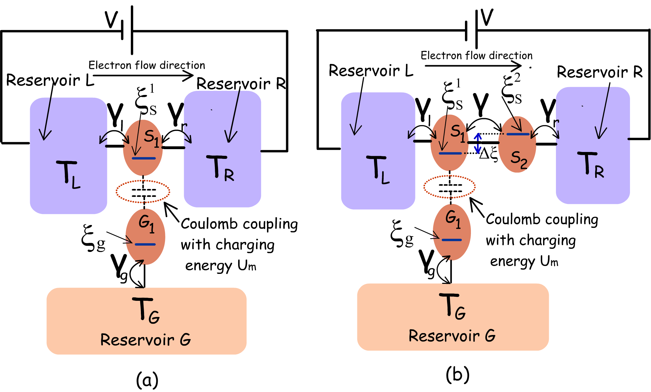
Figure 1: Schematic of the dual dot and triple dot thermometer (a) Schematic diagram of the dual dot thermometer based on Coulomb-coupled systems Zhang and Chen [2019]. This thermometer set-up is based on a simpler thermodynamic engine proposed by Sánchez et. al. Sánchez and Büttiker [2011a] and consists of two Coulomb-coupled quantum dots $S_{1}$ and $G_{1}$. $S_{1}$ is electrically connected to the reservoirs $L$ and $R$ and provides the path for current flow. $G_{1}$ on the other hand, is electrically connected to the remote reservoir $G$ whose temperature is to be accessed. To investigate the optimal performance of the dual dot thermometer, I choose $\gamma_{L}(\xi)=\gamma_{c}\theta(\xi_{s}^{1}+\delta\xi-\xi)$, $\gamma_{R}(\xi)=\gamma_{c}\theta(\xi-\xi_{s}^{1}-\delta\xi)$ and $\gamma_{g}(\xi)=\gamma_{c}$ Sánchez and Büttiker [2011a] with $\gamma_{c}=10\upmu$eV. Here, $\theta$ is the Heaviside step function and $\delta\xi<U_{m}$. (b) Schematic diagram of the proposed triple dot electrical thermometer. The entire system consists of the dots $S_{1}$, $S_{2}$ and $G_{1}$, which are electrically coupled to reservoirs L, R, and G respectively. $S_{1}$ and $G_{1}$ are capacitively coupled to each other (with Coulomb-coupling energy $U_{m}$). The ground state energy levels of the three dots $S_{1}$, $S_{2}$ and $G_{1}$ are denoted by $\xi_{s}^{1}$, $\xi_{s}^{2}$ and $\xi_{g}$ respectively. $S_{1}$ and $S_{2}$ share a staircase ground state configuration with $\xi_{s}^{2}=\xi_{s}^{1}+\Delta\xi$. To assess the optimal performance of the triple dot thermometer, I choose $\Delta E=U_{m}$ and $\gamma_{L}(\xi)=\gamma_{r}(\xi)=\gamma_{g}(\xi)=\gamma_{c}$, with $\gamma_{c}=10\upmu$eV.

II Performance parameters of the thermometers

The two types of non-local thermometers recently proposed in literature include (i) open-circuit voltage based thermometers Zhang and Chen [2019], and (ii) current based thermometers Yang et al. [2019]. Both of these thermometers rely on Coulomb coupling. The parameter employed to gauge the thermometer performance should be related to the rate of change of an electrical variable with temperature and is termed as sensitivity. As such, sensitivity is defined as the rate of change in (i) open-circuit voltage with temperature $\left(\frac{dV_{o}}{dT_{G}}\right)$ for voltage based thermometry and, (ii) current with temperature $\left(\chi=\frac{dI}{dT_{G}}\right)$ for current based thermometry. Here, $T_{G}$ is the remote target reservoir temperature to be assessed. When it comes to current based thermometry, a second parameter of importance, related to the efficiency, may be defined as the sensitivity per unit power dissipation, which I term as the performance coefficient. Thus, performance coefficient is given by:

$$Performance-coefficient=\frac{\chi}{P},$$ (1)

where $P=V\times I$ is the power dissipated across the set-up. In the above equation, $I$ indicates the current flowing through the thermometer on application of bias voltage $V$. It should be noted that the performance coefficient is a parameter to gauge the sensitivity with respect to power dissipation and is not a true efficiency parameter in sense of energy conversion.

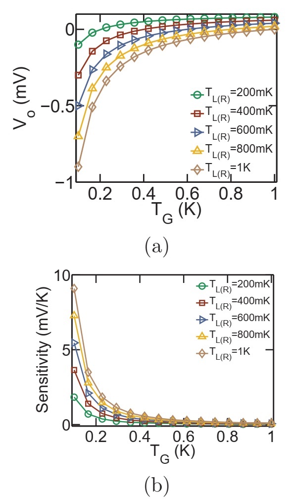
Figure 2: Voltage based thermometry in the dual-dot set-up depicted in Fig. 1(a). Variation in (a) Open-circuit voltage (b) temperature sensitivity $\left(\frac{dV_{o}}{dT_{G}}\right)$ with $T_{G}$ for different values of $T_{L(R)}$. For the above set of plots, the value of Coulomb coupling energy is chosen as $U_{m}=100\upmu$eV and the ground states are pinned at the equilibrium Fermi energy, that is, $\xi_{s}^{1}=\xi_{g}=\mu_{0}$. The open-circuit voltage as well as temperature sensitivity $\left(\frac{dV_{o}}{dT_{G}}\right)$ in the set-up under consideration is dependent on $T_{L(R)}$.

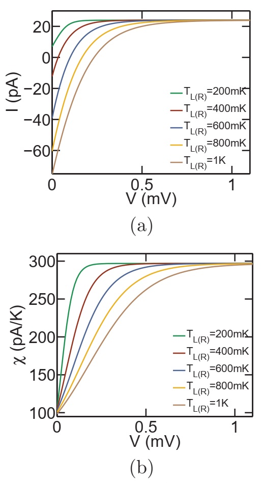
Figure 3: Current based thermometry in the dual-dot set-up depicted in Fig. 1(a). Variation in (a) total current (b) temperature sensitivity $\left(\chi=\frac{dI}{dT_{G}}\right)$ with applied bias $V$ for different values of $T_{L(R)}$. For the above set of plots, the parameters employed are $U_{m}=100\upmu$eV and $T_{G}=300$mK, while the ground states of $S_{1}$ and $G_{1}$ are pinned at the equilibrium Fermi energy, that is $\xi_{s}^{1}=\xi_{g}=\mu_{0}$. Given sufficiently high bias voltage $V$, the total current as well as temperature sensitivity $\chi=\left(\frac{dI}{dT_{G}}\right)$ saturate to the same value for different $T_{L(R)}$.

III Results

In this section, I investigate non-local open-circuit voltage and current based thermometry in the dual dot set-up. Proceeding further, I propose a triple dot design that demonstrates a superior sensitivity while circumventing the demand for any change in the system-to-reservoir coupling. In addition, the triple dot thermometer also demonstrates robustness against fabrication induced variability in Coulomb coupling. The performance and operation regime in case of current based sensitivity for both the dual dot and the triple dot thermometers were investigated and compared. The last part of this section investigates the thermometry induced refrigeration (heat-up) of the remote reservoir in the dual and triple dot set-up and also elaborates a strategy to reduce such undesired effect in case of the triple dot design.

III.1 Thermometry in the dual dot set-up

The dual dot thermometer, schematically demonstrated in Fig. 1(a), is based on the non-local thermodynamic engine originally conceived by Sánchez, et. al. Sánchez and Büttiker [2011a]. It consists of two quantum dots $S_{1}$ and $G_{1}$. The dot $S_{1}$ is electrically tunnel coupled to reservoirs L and R, while $G_{1}$ is electrically coupled to the reservoir G. Here, $G$ is the target reservoir whose temperature is to be assessed. The temperature of the reservoirs $L,~{}R$ and $G$ are symbolized as $T_{L},~{}T_{R}$ and $T_{G}$ respectively. The dots $S_{1}$ and $G_{1}$ are capacitively coupled with Coulomb coupling energy $U_{m}$, which permits exchange of electrostatic energy between the dots $S_{1}$ and $G_{1}$ while prohibiting any flow of electrons between them, resulting in zero net electronic current out of (into) the reservoir $G$. Thus the reservoir $G$ is electrically isolated from the current flow path. The ground state energy levels of the dots $S_{1}$ and $G_{1}$ are indicated by $\xi_{s}^{1}$ and $\xi_{g}$ respectively. Due to mutual Coulomb coupling between $S_{1}$ and $G_{1}$, the change in electron number $n_{S_{1}}~{}(n_{G_{1}})$ of the dot $S_{1}$ ($G_{1}$) influences the electrostatic energy of the dot $G_{1}$ ($S_{1}$). Under the assumption that the change in potential due to self-capacitance is much greater than the applied voltage $V$ or the average thermal voltage $kT/q$, that is $q^{2}/C_{self}>>(qV,k_{B}T)$, the electron occupation probability or transfer rate via the Coulomb blocked energy level, due to self-capacitance can be neglected Sánchez and Büttiker [2011a]. Thus, the system analysis can be approximated by considering four multi-electron levels by limiting the maximum number of electrons in the ground state of each quantum dot to $1$. Denoting each state by the electron occupation number in the quantum dot ground state, a possible system state of interest may be represented as $\ket{n_{S_{1}},n_{G_{1}}}=\ket{n_{S_{1}}}\mathbin{\mathop{\otimes}\limits}\ket{n_{G_{1}}}$, where $n_{S_{1}},n_{G_{1}}\in(0,1)$, denote the number of electrons present in the ground-states of $S_{1}$ and $G_{1}$ respectively. The above assumptions validate the use of the quantum master equations (QME) employed in Ref. Sánchez and Büttiker [2011a] for investigation of an equivalent set-up. It was demonstrated in Refs. Sánchez and Büttiker [2011a]; Zhang and Chen [2019] that optimal operation of the dual-dot based set-up as heat engine and thermometer demands an asymmetric step-like system-to-reservoir coupling. Hence, to investigate the optimal performance of the dual dot thermometer, I choose $\gamma_{l}(\xi)=\gamma_{c}\theta(\xi_{s}^{1}+\delta\xi-\xi)$and $\gamma_{r}(\xi)=\gamma_{c}\theta(\xi-\xi_{s}^{1}-\delta\xi)$ Sánchez and Büttiker [2011a] with $\gamma_{c}=10\upmu$eV and $\delta\xi<U_{m}$. Here, $\theta$ and $\xi$ respectively are the Heaviside step function and the free-variable denoting energy. In addition, I choose $\gamma_{g}=\gamma_{c}$. Such order of coupling parameter correspond to realistic experimental values in Ref. Thierschmann et al. [2015a], where the system-to-reservoir coupling was evaluated, from experimental data, to lie in the range of $20\sim 50\upmu$eV. In addition, such order of the coupling parameters also indicate weak coupling and limit the electronic transport in the sequential tunneling regime where the impact of cotunneling and higher-order tunneling processes can be neglected. Unless stated, the temperature of the reservoirs $L$ and $R$ are assumed to be $T_{L(R)}=300$mK. To assess the performance of the thermometer, I follow the approach as well as the quantum master equations employed in Refs. Sánchez and Büttiker [2011a]; Zhang et al. [2015a], where the probability of occupancy of the considered multi-electron states were evaluated via well established quantum master equations (QME) to finally calculate the charge and heat currents through the system.
Voltage-based thermometry: In case of non-local thermoelectric voltage based thermometry, the applied bias $V$ in Fig. 1(a) is replaced by open circuit and the voltage between the terminals $L$ and $R$ is measured. Such open circuit voltage based thermometry for the considered dual dot set-up was analyzed earlier in detail by Zhang, et. al. Zhang and Chen [2019]. I plot, in Fig. 2, the variation in open-circuit voltage ($V_{o}$) and temperature sensitivity $\left(\frac{dV_{o}}{dT_{G}}\right)$ for different values of $T_{L(R)}$ at $U_{m}=100\upmu$eV. It is evident that the open-circuit voltage as well as sensitivity $\left(\frac{dV_{o}}{dT_{G}}\right)$ in such a set-up is dependent on $T_{L(R)}$, which makes it non-robust against fluctuations in the measurement terminal temperature. The variation in open-circuit voltage and sensitivity with $T_{L(R)}$ results from the fact that non-local thermoelectric voltage developed in such set-ups is dependent on $\Delta T=T_{L(R)}-T_{G}$.

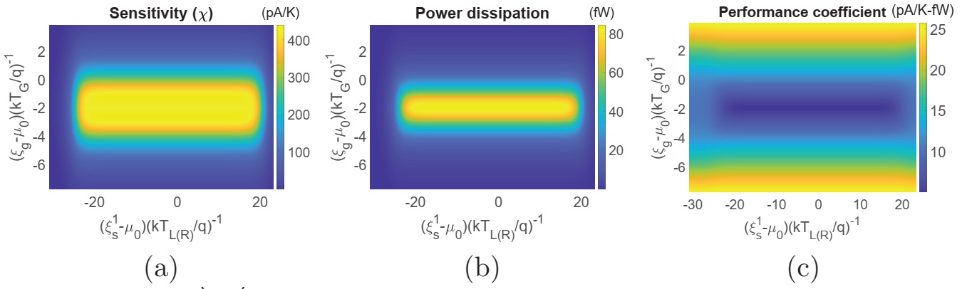
Figure 4: Regime of operation of the dual dot set-up in terms of the ground state energy positions relative to the equilibrium Fermi energy $\mu_{0}$. Colour plot demonstrating the variation in (a) sensitivity ($\chi$) (b) power dissipation and (c) performance coefficient with variation in the ground state positions $\xi_{s}^{1}$ and $\xi_{g}$. The parameters used for simulation are $U_{m}=100\upmu$eV, $\gamma_{c}=10\upmu$eV, $V=1.1$mV and $T_{L(R)}=T_{G}=300$mK.

Current-based thermometry: To ensure robustness in such a set-up against fluctuation and variation in measurement terminal temperature and voltage, current based thermometry offers an alternative method. In this case, a bias voltage $V$ is applied between the reservoirs $L$ and $R$ and temperature of the reservoir $G$ can be assessed via the current measurement. As stated before, temperature sensitivity in this case is defined as

$$\chi=\frac{dI}{dT_{G}},$$ (2)

where $I$ is the electronic current flowing between the reservoirs $L$ and $R$. Fig. 3 demonstrates the variation in electronic current $I$ and temperature sensitivity $\chi=\left(\frac{dI}{dT_{G}}\right)$ for different values of $T_{L(R)}$ at $U_{m}=100\upmu$eV. It should be noted that the set-up is affected by non-local thermoelectric action in the regime of low bias, which is evident from different magnitudes of current at distinct values of $T_{L(R)}$. However, for sufficiently high bias voltage, the electronic current as well as the sensitivity $\chi=\left(\frac{dI}{dT_{G}}\right)$ saturate to a finite limit for different values of $T_{L(R)}$. Thus, in the regime of high bias, current based thermometry in the set-up under consideration is robust against thermoelectric effect, fluctuations in the bias voltage and variation in measurement terminal temperature $T_{L(R)}$.
Fig. 4 demonstrates the regime of operation of the set-up under consideration with respect to the ground state energy positions for $U_{m}=100\upmu$eV, $V=1.1$mV and $T_{L(R)}=T_{G}=300$mK. Such values of the applied bias drive the thermometer in the regime of maximum saturation sensitivity. In particular, Fig. 4(a) demonstrates the variation in sensitivity ($\chi$) with ground state positions $\xi_{s}^{1}$ and $\xi_{g}$ relative to the equilibrium Fermi level $\mu_{0}$. We note that the optimal sensitivity is obtained when $\xi_{g}$ lies within the range of a few $kT_{G}$ below the equilibrium Fermi energy $\mu_{0}$. This is because, the flow of an electron from reservoir $L$ to $R$ demands the entry of an electron in dot $G_{1}$ at energy $\xi_{g}+U_{m}$ and subsequently exit of the electron from $G_{1}$ into reservoir $G$ at an energy $\xi_{g}$ Sánchez and Büttiker [2011a]; Zhang et al. [2015a]. To understand this, let us consider the complete cycle that transfers an electron from reservoir $L$ to $R$ in the dual dot set-up: $\ket{0,0}\rightarrow\ket{1,0}\rightarrow\ket{1,1}\rightarrow\ket{0,1}\rightarrow\ket{0,0}$. In this cycle, an electron tunnels into the dot $S_{1}$ from reservoir $L$ at energy $\xi_{s}^{1}$. Next, an electron tunnels into the dot $G_{1}$ from reservoir $G$ at energy $\xi_{g}+U_{m}$. In the following step, the electron in $S_{1}$ tunnels out into the reservoir $R$ at energy $\xi_{s}^{1}+U_{m}$. The system returns to the vacuum state, that is $\ket{0,0}$ when the electron in $G_{1}$ tunnels out into reservoir $G$ at energy $\xi_{g}$. Thus, the sensitivity becomes optimal in the regime around the maximum value of the factor $\frac{d}{dT_{G}}\left[f\left(\frac{\xi_{g}+U_{m}-\mu_{0}}{kT_{G}}\right)\left\{1-f\left(\frac{\xi_{g}-\mu_{0}}{kT_{G}}\right)\right\}\right]$, which occurs when $\xi_{g}$ is a few $kT_{G}$ below the equilibrium Fermi energy $\mu_{0}$. Similarly, the power dissipation, shown in Fig. 4(b), is high when $\xi_{g}$ lies within the range of a few $kT_{G}$ below the equilibrium Fermi energy $\mu_{0}$ due to high current flow. Interestingly, by comparing Fig. 4(a) and (b), we find regimes where the sensitivity is high at a relatively lower power dissipation. The performance coefficient (shown in Fig. 4.c), on the other hand, is low in the regime of high sensitivity and increases as $\xi_{g}$ deviates from the equilibrium Fermi energy beyond a few $kT_{G}$. This can be explained as follows. In the regime of high sensitivity, the current flow is high. Due to limited current carrying capacity of the dual dot set-up, the rate of fractional increase in current flow with $T_{G}$, that is $\left(\frac{1}{I}\frac{dI}{dT_{G}}\right)$, is lower in the regime of high current flow. Hence, although the sensitivity is high, the rate of fractional increase in current flow with temperature, and hence the sensitivity per unit power dissipation is lower. This gives rise to low performance coefficient. On the other hand, in the regime of low sensitivity, the current flow is lower (evident from the lower power dissipation). Thus, the rate of fractional increase in current flow with $T_{G}$, that is $\left(\frac{1}{I}\frac{dI}{dT_{G}}\right)$, is higher in this regime. This gives rise to high performance coefficient in the regime of low sensitivity. From Fig. 4(a-c), we also note that the sensitivity, power dissipation and performance coefficient is fairly constant over a wide range of $\xi_{s}^{1}$. Although not shown here, this range depends on and increases (decreases) with the increase (decrease) in the applied bias voltage.

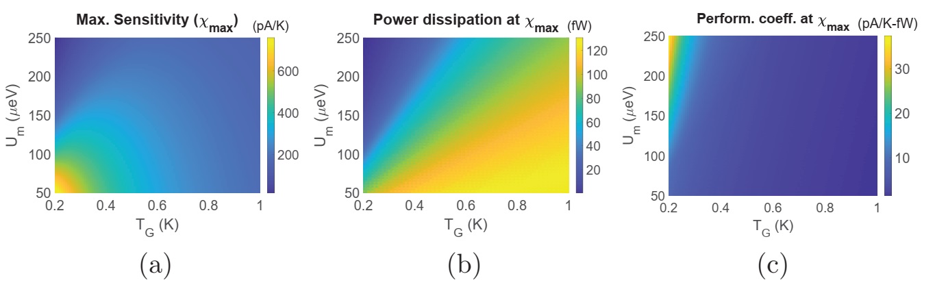
Figure 5: Maximum sensitivity and parameters at maximum sensitivity for the dual dot thermometer. Colour plot demonstrating the variation in (a) maximum sensitivity ($\chi_{max}$) (b) power dissipation at maximum sensitivity and (c) performance coefficient at maximum sensitivity with variation in the Coulomb coupling energy ($U_{m}$) and target reservoir temperature ($T_{G}$). The parameters used for simulation are $T_{L(R)}=300$mK, $\gamma_{c}=10\upmu$eV and $V=1.1$mV.

I demonstrate in Fig. 5, the variation in maximum sensitivity ($\chi_{max}$), as well as, power dissipation and performance coefficient at the maximum sensitivity with variation in the Coulomb coupling energy ($U_{m}$) and $T_{G}$ respectively. To calculate the maximum sensitivity and related parameters at the maximum sensitivity, the ground states are tuned to optimal positions with respect to the equilibrium Fermi energy ($\mu_{0}$). We note that the maximum sensitivity, shown in Fig. 5(a), is relatively higher in the regime of low Coulomb coupling energy $U_{m}$ and decreases with $U_{m}$. This is because the maximum value of $\frac{d}{dT_{G}}\left[f\left(\frac{\xi_{g}+U_{m}-\mu_{0}}{kT_{G}}\right)\left\{1-f\left(\frac{\xi_{g}-\mu_{0}}{kT_{G}}\right)\right\}\right]$ decreases with increase in $U_{m}$. Moreover, we also note that the sensitivity changes non-monotonically with $T_{G}$. Coming to the aspect of power dissipation, we note that the dissipated power at the maximum sensitivity decreases monotonically with $U_{m}$. This, again, is due to decrease in the optimal value of the product $f\left(\frac{\xi_{g}+U_{m}-\mu_{0}}{kT_{G}}\right)\left\{1-f\left(\frac{\xi_{g}-\mu_{0}}{kT_{G}}\right)\right\}$ with $U_{m}$, which results in decrease in the current flow and, hence power dissipation. In addition, the power dissipation also increases with $T_{G}$ for the same reason of increase in current due to increase in the product $f\left(\frac{\xi_{g}+U_{m}-\mu_{0}}{kT_{G}}\right)\left\{1-f\left(\frac{\xi_{g}-\mu_{0}}{kT_{G}}\right)\right\}$ with $T_{G}$. The performance coefficient at the maximum sensitivity, as noted from Fig. 5(c), is maximum in the regime of low temperature and high Coulomb coupling energy $U_{m}$, rendering this set-up suitable for applications in the “sub-Kelvin” temperature regime.

III.2 Thermometry in triple-dot set-up

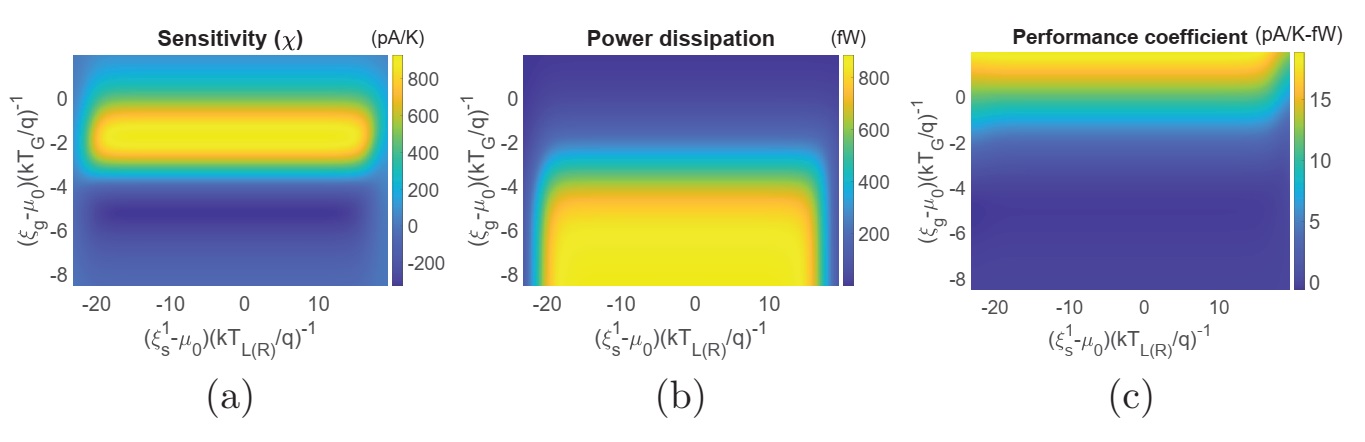
Figure 6: Regime of operation of the proposed triple dot thermometer in terms of the ground state energy positions relative to the equilibrium Fermi energy $\mu_{0}$. Colour plot demonstrating the variation in (a) sensitivity ($\chi$) (b) power dissipation and (c) performance coefficient with variation in the ground state positions $\xi_{s}^{1}$ and $\xi_{g}$. The parameters used for simulation are $U_{m}=100\upmu$eV, $\gamma_{c}=10\upmu$eV, $V=1.1$mV and $T_{L(R)}=T_{G}=300$mK.

Proposed set-up configuration and transport formulation: The triple dot thermometer, proposed in this paper, is schematically demonstrated in Fig. 1(b) and consists of three dots $S_{1},~{}S_{2}$ and $G_{1}$ which are electrically coupled to the reservoirs $L$, $R$ and $G$ respectively. Compared to the dual-dot design, the triple dot set-up features an extra quantum dot $S_{2}$ between $S_{1}$ and reservoir $R$. Coming to the ground state configuration and other features of the system, $S_{1}$ and $S_{2}$ are tunnel coupled to each other, while $G_{1}$ is capacitively coupled to $S_{1}$. The ground states of $S_{1}$ and $S_{2}$ form a stair-case configuration with $\xi_{s}^{2}=\xi_{s}^{1}+\Delta\xi$. Any electronic tunneling between the dots $S_{1}$ and $G_{1}$ is suppressed via suitable fabrication techniques Hübel et al. [2007]; Chan et al. [2002]; Molenkamp et al. [1995]; Hübel et al. [2008]; Ruzin et al. [1992]. Energy exchange between $S_{1}$ and $G_{1}$ is, however, feasible via Coulomb coupling Hübel et al. [2007]; Chan et al. [2002]; Molenkamp et al. [1995]; Hübel et al. [2008]; Ruzin et al. [1992]. In the optimal dual-dot thermometer discussed above, an asymmetric step-like system-to-reservoir coupling is required for optimal operation. In the proposed triple-dot thermometer, the asymmetric system-to-reservoir coupling is bypassed by choosing an energy difference between the ground states of $S_{1}$ and $S_{2}$ which makes the system asymmetric with respect to the reservoir $L$ and $R$. Another equivalent triple-dot set-up, based on Coulomb coupled systems, that can be employed for efficient non-local thermometry is demonstrated in Fig. 12 and discussed briefly in Appendix A. Coming to the realistic fabrication possibility of such a system, due to the recent advancement in solid-state nano-fabrication technology, triple and quadruple quantum dot systems with and without Coulomb coupling have already been realized experimentally Eng et al. [2015]; Flentje et al. [2017]; Froning et al. [2018]; Noiri et al. [2017]; Hong et al. [2018]; Takakura et al. [2014]. In addition, it has been experimentally demonstrated that quantum dots that are far from each other in space, may be bridged to obtain strong Coulomb coupling, along with excellent thermal isolation between the reservoirs which may be at different temperatures Hübel et al. [2007]; Chan et al. [2002]; Molenkamp et al. [1995]; Hübel et al. [2008]; Ruzin et al. [1992]. Also, the bridge may be fabricated between two specific quantum dots to drastically enhance their mutual Coulomb coupling, without affecting the electrostatic energy of the other quantum dots in the system Hübel et al. [2007]; Chan et al. [2002]; Molenkamp et al. [1995]; Hübel et al. [2008]; Ruzin et al. [1992]. Due to mutual Coulomb coupling between $S_{1}$ and $G_{1}$, the change in electron number $n_{S_{1}}~{}(n_{G_{1}})$ of the dot $S_{1}$ ($G_{1}$) influences the electrostatic energy of the dot $G_{1}$ ($S_{1}$). The total increase in electrostatic energy $U$ of the triple dot configuration, demonstrated in Fig. 1 (b), due to deviation in electronic number from the minimum energy configuration can be given by (Appendix B):

$$U(n_{S_{1}},n_{G_{1}},n_{S_{2}})=\sum_{x}U^{self}_{x}\left(n_{x}^{tot}-n_{x}^{eq}\right)^{2}+\sum_{(x_{1},x_{2})}^{x_{1}\neq x_{2}}U^{m}_{x_{1},x_{2}}\left(n_{x_{1}}^{tot}-n_{x_{1}}^{eq}\right)\left(n_{x_{2}}^{tot}-n_{x_{2}}^{eq}\right)$$ (3)

where $n_{x}^{tot}$ is the total electron number, and $U^{self}_{x}=\frac{q^{2}}{C^{self}_{x}}$ is the electrostatic energy due to self-capacitance $C^{self}_{x}$ (with the surrounding leads) of quantum dot ‘$x$’ (See Appendix B for details). $U^{m}_{x_{1},x_{2}}$ is the electrostatic energy arising out of Coulomb coupling between two different quantum dots $x_{1}$ and $x_{2}$, where a change in electron number in $x_{1}$ affects the electrostatic energy in $x_{2}$ or vice-versa (Appendix B). $n_{x}^{eq}$ is the total number of electrons in dot $x$ under equilibrium condition at $0K$ and is determined by the lowest possible electrostatic energy of the system. Hence, $n_{x}=n_{x}^{tot}-n_{x}^{eq}$ is the total number of electrons in the ground state of the dot $x$ due to application of bias voltage or stochastic fluctuations from the reservoirs (Details given in Appendix B). Under the assumption that the change in potential due to self-capacitance is much greater than than the average thermal voltage $kT/q$ or the applied bias voltage $V$, that is $U^{self}_{x}=\frac{q^{2}}{C^{self}_{x}}>>(kT,~{}qV)$, the electron occupation probability or transfer rate via the Coulomb blocked energy level, due to self-capacitance, is negligibly small. Under such a condition, the analysis of the triple dot system can be approximated by limiting the maximum number of electrons in each dot to unity. So, there are $2^{3}=8$ multi-electron levels which characterize the entire non-equilibrium properties of the set-up. I denote each of these states by the ground state occupation number in each quantum dot. Hence, a possible state of interest in the system may be denoted as $\ket{n_{S_{1}},n_{G_{1}},n_{S_{2}}}=\ket{n_{S_{1}}}\mathbin{\mathop{\otimes}\limits}\ket{n_{G_{1}}}\mathbin{\mathop{\otimes}\limits}\ket{n_{S_{2}}}$, where $n_{S_{1}},n_{G_{1}},n_{S_{2}}\in(0,1)$, denote the number of electrons present in the ground-states of $S_{1},~{}G_{1}$ and $S_{2}$ respectively. I also neglect electrostatic coupling between $S_{1},~{}S_{2}$ and $S_{2},~{}G_{1}$ for all practical purposes under consideration. Due to mutual coupling, the ground states as well as electronic transport in $S_{1}$ and $G_{1}$ are inter-dependent and hence, I treat the pair of dots $S_{1}$ and $G_{1}$ as a sub-system ($\varsigma_{1}$), $S_{2}$ being the complementary sub-system ($\varsigma_{2}$) of the entire triple-dot set-up (Appendix B). The state probability of $\varsigma_{1}$ is denoted by $P_{i,j}^{\varsigma_{1}}$, $i$ and $j$ being the ground state electron number of dot $S_{1}$ and $G_{1}$ respectively. $P_{k}^{\varsigma_{2}}$, on the other hand, denotes the probability of occupancy of the dot $S_{2}$ in the complementary sub-system $\varsigma_{2}$. It can be shown that if $\Delta\xi$ is much greater than the system-to-reservoir coupling, that is $\Delta\xi>>\gamma_{c}$, then the interdot tunneling rate between $S_{1}$ and $S_{2}$ becomes maximum under the condition $\xi_{s}^{1}+U^{m}_{S_{1},G_{1}}=\xi_{s}^{2}$, that is when $\Delta\xi=U^{m}_{S_{1},G_{1}}$ (Appendix B). To investigate the optimal performance of the proposed thermometer, I hence assume $\Delta\xi=U^{m}_{S_{1},G_{1}}$. In the following discussion, I would simply represent $U^{m}_{S_{1},G_{1}}$ as $U_{m}$. Under the above set of assumptions, the equations dictating sub-system steady-state probabilities are given by (Appendix B):

$$-P_{0,0}^{\varsigma_{1}}\{f_{L}(\xi_{s}^{1})+f_{G}(\xi_{g})\}+P_{0,1}^{\varsigma_{1}}\{1-f_{G}(\xi_{g})\}+P_{1,0}^{\varsigma_{1}}\{1-f_{L}(\xi_{s}^{1})\}=0$$

$$-P_{1,0}^{\varsigma_{1}}\left\{1-f_{L}(\xi_{s}^{1})+f_{G}(\xi_{g}+U_{m})\right\}+P_{1,1}^{\varsigma_{1}}\left\{1-f_{G}(\xi_{g}+U_{m})\right\}+P_{0,0}^{\varsigma_{1}}f_{L}(\xi_{s}^{1})$$

$$-P_{0,1}^{\varsigma_{1}}\left\{1-f_{g}(\xi_{g}^{1})+f_{L}(\xi_{s}^{1}+U_{m})+\frac{\gamma}{\gamma_{c}}P^{\varsigma_{2}}_{1}\right\}+P_{0,0}^{\varsigma_{1}}f_{G}(\xi_{g})+P_{1,1}^{\varsigma_{1}}\left\{1-f_{L}(\xi_{s}^{1}+U_{m})+\frac{\gamma}{\gamma_{c}}P^{\varsigma_{2}}_{0}\right\}=0$$

$$-P_{1,1}^{\varsigma_{1}}\left\{[1-f_{g}(\xi_{g}^{1}+U_{m})]+[1-f_{L}(\xi_{s}^{1}+U_{m})]+\frac{\gamma}{\gamma_{C}}P^{\varsigma_{2}}_{0}\right\}+P_{1,0}^{\varsigma_{1}}f_{G}(\xi_{g}+U_{m})+P_{0,1}^{\varsigma_{1}}\left\{f_{L}(\xi_{s}^{1}+U_{m})+\frac{\gamma}{\gamma_{c}}P^{\varsigma_{2}}_{1}\right\}=0$$ (4)

$$-P_{0}^{\varsigma_{2}}\{f_{R}(\xi_{s}^{2})+\frac{\gamma}{\gamma_{c}}P_{1,1}^{\varsigma_{1}}\}+P_{1}^{\varsigma_{2}}\left\{1-f_{R}(\xi_{s}^{2})+\frac{\gamma}{\gamma_{c}}P^{\varsigma_{1}}_{0,1}\right\}=0$$

$$-P_{1}^{\varsigma_{2}}\{1-f_{R}(\xi_{s}^{2})+\frac{\gamma}{\gamma_{c}}P^{\varsigma_{1}}_{0,1}\}+P_{0}^{\varsigma_{2}}\left\{f_{R}(\xi_{s}^{2})+\frac{\gamma}{\gamma_{c}}P_{1,1}^{\varsigma_{1}}\right\}=0,$$ (5)

where $\gamma_{l}(\xi)=\gamma_{r}(\xi)=\gamma_{g}(\xi)=\gamma_{c}$ and $\gamma$ are related to the reservoir-to-system tunnel coupling and the inter-dot tunnel coupling respectively Datta [2005], $\xi$ being the independent energy variable. In the above set of equations, $f_{\lambda}(\xi)$ denotes the probability of occupancy of the reservoir $\lambda$ at energy $\xi$. For the purpose of calculations in this paper, I assume a quasi-equilibrium Fermi-Dirac statistics at the reservoirs. Hence, $f_{\lambda}(\xi)$ is given by:

$$f_{\lambda}(\xi)=\left(1+exp\left\{\frac{\xi-\mu_{\lambda}}{kT_{\lambda}}\right\}\right)^{-1},$$ (6)

where $\mu_{\lambda}$ and $T_{\lambda}$ respectively denote the quasi-Fermi energy and temperature of the reservoir $\lambda$. From the set of Eqns. (4) and (5), it is clear that an electron in $S_{1}$ can tunnel into $S_{2}$ only when the ground state in the dot $G_{1}$ is occupied with an electron. The set of Eqns. (4) and (5) are coupled to each other and may be solved using any iterative method. Here, I use Newton-Raphson iterative method to solve the steady-state values of sub-system probabilities. On calculation of the sub-system state probabilities $P_{i,j}^{\varsigma_{1}}$ and $P_{k}^{\varsigma_{2}}$, the electron current flow into (out of) the system from the reservoirs $L(R)$ can be given as:

$$I_{L}= q\gamma_{c}\times\left\{P^{\varsigma_{1}}_{0,0}f_{L}(\xi_{s}^{1})+P^{\varsigma_{1}}_{0,1}f_{L}(\xi_{s}^{1}+U_{m})\right\}$$

$$-q\gamma_{c}P^{\varsigma_{1}}_{1,0}\{1-f_{L}(\xi_{s}^{1})\}-q\gamma_{c}P^{\varsigma_{s}^{1}}_{1,1}\{1-f_{L}(\xi_{s}^{1}+U_{m})\}$$

$$I_{R}= -q\gamma_{c}\times\left\{P^{\varsigma_{2}}_{0}f_{R}(\xi_{s}^{1})-P^{\varsigma_{2}}_{1}\{1-f_{R}(\xi_{s}^{1})\}\right\},$$ (7)

In addition, the electronic component of heat flow from the reservoir $G$ can be given by:

$$I_{Qe}=U_{m}\gamma_{c}\left\{P^{\varsigma_{1}}_{10}f_{G}(\xi_{g}+U_{m})-P^{\varsigma_{1}}_{11}\{1-f_{G}(\xi_{g}+U_{m})\}\right\}$$ (8)

Interestingly, we note that Eqn. (8) is not directly dependent on $\xi_{g}$. This is due to the fact that the net electronic current into or out of the reservoir $G$ is zero (See Appendix B for details).

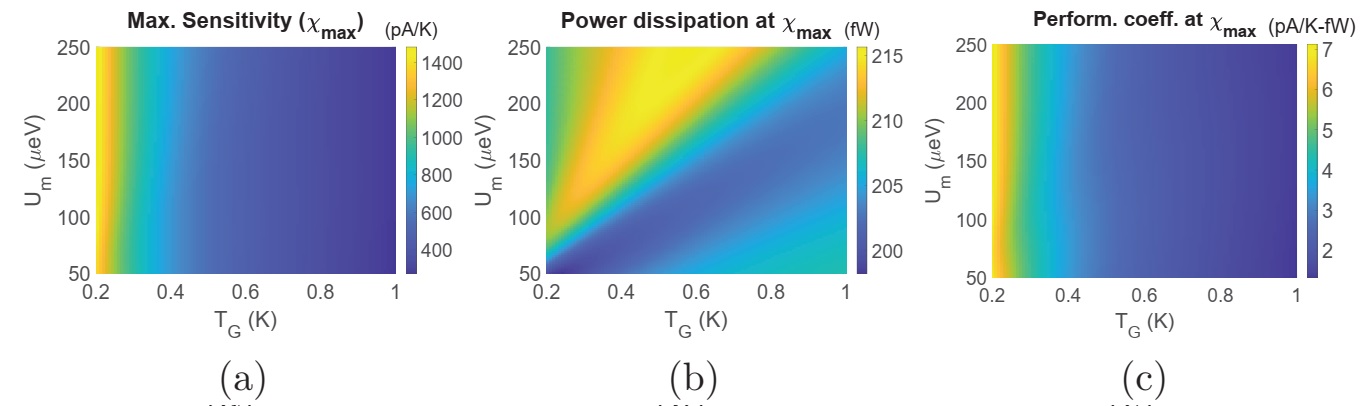
Figure 7: Maximum sensitivity and parameters at maximum sensitivity for the triple dot thermometer. Colour plot demonstrating the variation in (a) maximum sensitivity ($\chi_{max}$) (b) power dissipation at maximum sensitivity and (c) performance coefficient at maximum sensitivity with variation in the Coulomb coupling energy ($U_{m}$) and target reservoir temperature ($T_{G}$). The parameters used for simulation are $T_{L(R)}=300$mK, $\gamma_{l}(\xi)=\gamma_{r}(\xi)=\gamma_{g}(\xi)=\gamma(\xi)=\gamma_{c}=10\upmu$eV and $V=1.1$mV.

Operation regime and performance investigation: For investigating the triple dot set-up, I choose the system-to-reservoir coupling as $\gamma_{l}(\xi)=\gamma_{r}(\xi)=\gamma_{g}(\xi)=\gamma_{c}$, with $\gamma_{c}=10\upmu$eV. In addition, I also choose the interdot coupling to be $\gamma(\xi)=10\upmu$eV. As stated earlier, such values of coupling parameters lie within experimentally feasible range Thierschmann et al. [2015a]. Fig. 6 demonstrates the regime of operation of the proposed triple dot thermometer. In particular, Fig. 6(a) depicts the sensitivity as a function of the ground state positions. We note that the sensitivity increases as $\xi_{g}$ gradually goes below the Fermi energy, with the maximum sensitivity occurring when $\xi_{g}-\mu_{0}\approx-1.5kT_{G}$. As $\xi_{g}$ goes further below the Fermi energy, the sensitivity becomes negative. This occurs when an increase in temperature decreases the probability of occupancy of both the ground state $\xi_{g}$ and the Coulomb blocked state $\xi_{g}+U_{m}$, that is when $\xi_{g}+U_{m}-\mu_{0}<0$. Despite the fact that this set-up offers the provision to implement a positively sensitive as well as a negatively sensitive thermometer, it should be noted from Fig. 6(b) that the power dissipation is very high in the negatively sensitive regime. This is due to the fact that when $\xi_{g}+U_{m}-\mu_{0}<0$, the occupancy probability of $G_{1}$ is very high, which causes a high drive current between reservoirs $L$ and $R$. The power dissipation in the regime of positive sensitivity is lower, resulting in a higher performance coefficient, as noted from Fig. 6(c). Also, the power dissipation and performance coefficient respectively decreases and increases as $\xi_{s}^{1}$ gradually approaches and finally moves above the equilibrium Fermi-energy. This is because as $\xi_{g}$ gradually approaches and goes above the Fermi energy, the probability of occupancy of $\xi_{g}$ becomes lower, blocking the current flow through the system. Due to the same reason as stated for the dual dot set-up, a lower current flow through the system leads to a higher fractional increase in current with the remote reservoir temperature $T_{G}$, leading to a higher performance coefficient. We also note from Fig. 6(a)-(c) that the sensitivity, power dissipation and performance coefficient remains almost constant for a wide range of $\xi_{s}^{1}$. As discussed before, this range depends on and increases (decreases) with increase (decrease) in applied bias voltage.

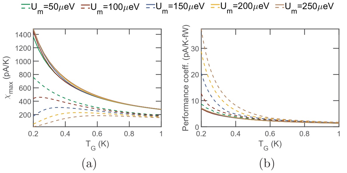
Figure 8: Performance comparison between the dual dot and the triple dot thermometer. Variation in (a) maximum sensitivity ($\chi_{max}$) and (b) Performance-coefficient at the maximum sensitivity with $T_{G}$ for different values of Coulomb coupling energy $U_{m}$. The solid and the dashed line represent the performance parameters of the triple dot and dual dot thermometers respectively. The system parameters used for simulation are $T_{L(R)}=300$mK, and $V=1.1$mV. For the dual dot thermometer, the different system to reservoir coupling are chosen to be $\gamma_{l}(\xi)=\gamma_{c}\theta(\xi_{s}^{1}+\delta\xi-\xi)$, $\gamma_{r}(\xi)=\gamma_{c}\theta(\xi-\xi_{s}^{1}-\delta\xi)$ and $\gamma_{g}=\gamma_{c}$. For the triple dot thermometer, the system to reservoir, as well as the interdot coupling are chosen to be $\gamma_{l}(\xi)=\gamma_{r}(\xi)=\gamma_{g}(\xi)=\gamma(\xi)=\gamma_{c}=10\upmu$eV. In both the dual dot and the triple dot thermometer, $gamma_{c}=10\upmu$eV.

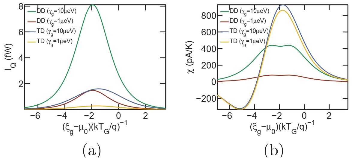
Figure 9: Analysis of thermometry induced refrigeration of the reservoir $G$ for the dual-dot (DD) and triple dot (TD) set-up. Plot of (a) heat current ($I_{Q}$) extracted from the reservoir $G$ and (b) sensitivity with variation in the ground state $\xi_{g}$. In case of the dual dot (DD) set-up, decreasing the system-to-reservoir coupling ($\gamma_{g}$) between $G$ and $G_{1}$ decreases both the extracted heat current $I_{Q}$ and sensitivity $\chi$. However, for the triple dot set-up, decreasing $\gamma_{g}$ suppresses only the heat current $I_{Q}$, while keeping the sensitivity ($\chi$) almost unaltered. The parameters used for simulation are $U_{m}=100\upmu$eV, $\gamma_{c}=10\upmu$eV, $T_{L(R)}=T_{G}=300$mK and $\xi_{s}^{1}=\mu_{0}$.

Fig. 7 demonstrates the maximum sensitivity ($\chi_{max}$) as well as the power dissipation and performance coefficient at the maximum sensitivity with variation in the Coulomb coupling energy $U_{m}$ and target reservoir temperature $T_{G}$. Just as before, to calculate the maximum sensitivity and related parameters at the maximum sensitivity, the quantum dot ground states are tuned to their optimal positions. Fig. 7(a) demonstrates the maximum sensitivity with variation in $U_{m}$ and $T_{G}$. An interesting thing to note is that the triple dot thermometer is fairly robust against variation in the Coulomb coupling energy $U_{m}$. This can be explained by the fact that current flow through the triple quantum dot set-up only demands the occupancy of the dot $G_{1}$ whose ground state can be tuned to optimum position for maximizing the sensitivity. Thus, optimal sensitivity can be achieved by placing $\xi_{g}$ around the energy $\xi$ at which the rate of change in ground state occupancy probability of $G_{1}$ is maximum with $T_{G}$. This condition is unlike the case of dual dot set-up where one has to maximize the factor $\frac{d}{dT_{G}}\left[f\left(\frac{\xi_{g}+U_{m}-\mu_{0}}{kT_{G}}\right)\left\{1-f\left(\frac{\xi_{g}-\mu_{0}}{kT_{G}}\right)\right\}\right]$ for achieving the maximum sensitivity. We also note that, unlike the dual dot set-up, the maximum sensitivity in this case decreases monotonically with $T_{G}$. The power dissipation, as demonstrated in Fig. 7(b), also remains almost constant and varies between $199$fW and $216$fW with variation in $U_{m}$ and $T_{G}$. This again is a result of the fact that current flow through the triple dot set-up only demands occupancy of the dot $G_{1}$ and thus the position of $\xi_{g}$ for maximum sensitivity induces a high current flow through the set-up. Due to almost constant power dissipation with variation in $U_{m}$ and $T_{G}$, the performance-coefficient also shows a similar trend as the sensitivity with $U_{m}$ and $T_{G}$, as noted in Fig. 7(c). It is evident from Fig. (4)-(7) that the triple dot thermometer demonstrates an enhanced sensitivity, but lower performance coefficient compared to the dual dot thermometer. As such, it is important to compare their performance, which leads us to the next discussion.

III.3 Performance comparison

To further shed light on the relative performance of the triple dot thermometer with respect to the dual dot thermometer, I plot in Fig. 8(a) and (b) the sensitivity and performance-coefficient respectively for the dual dot (dashed lines) and the triple dot (solid lines) thermometers respectively. As stated earlier, the triple dot thermometer demonstrates an enhanced sensitivity and offers significant advantage, particularly in the regime of high Coulomb coupling energy $U_{m}$. This is due to the fact that each electronic flow between reservoirs $L$ and $R$ in the dual dot set-up demands an electron entrance and exit from $G_{1}$ at energy $\xi_{g}+U_{m}$ and $\xi_{g}$ respectively. Thus, the probability of electronic flow is significantly reduced, particularly for high $U_{m}$. Electronic flow in the triple dot set-up on the other hand demands only occupancy of the dot $G_{1}$, which can be achieved by positioning the ground state $\xi_{g}$ appropriately with respect to the equilibrium Fermi energy. Thus, this system eliminates the dependence of sensitivity on $U_{m}$, making it fairly robust against fabrication induced variability in the Coulomb coupling energy. The performance coefficient of the triple dot set-up, on the other hand, is lower compared to the dual dot thermometer. This is due to high current flow in the triple dot thermometer and becomes particularly noticeable in the regime of high values of $U_{m}$, where the dual dot set-up hosts very less current flow and sensitivity but high performance coefficient. It should be noted that the performance coefficient offered by the triple dot thermometer is reasonable and approaches that of the dual dot set-up in the higher temperature regime.

III.4 Thermometry induced refrigeration

It is well known that the transfer of each electron from reservoir $R$ to $L$, in the dual dot set-up, demands extraction of a heat packet $U_{m}$ from reservoir $G$ Sánchez and Büttiker [2011a]; Zhang et al. [2015a]. This means that increasing the system-to-reservoir coupling to achieve enhanced sensitivity would also result in extraction of more heat packets from reservoir $G$. Such a phenomena may result in unnecessary refrigeration or temperature drift of the reservoir $G$ in an undesirable manner. Since, the number of heat packets extracted in this set-up is exactly equal to the number of electrons that flow between reservoir $L$ and $R$ ($I_{Q}=IU_{m}/q$), reducing $\gamma_{g}$ to suppress the refrigeration of reservoir $G$ also results in the reduction of sensitivity. This is shown in Fig. 9(a) and (b), where it is demonstrated that reduction in $\gamma_{g}$ for the dual dot (DD) set-up, by a factor of $10$, results in suppression of both the maximum heat current ($I_{Q}$) from $8.1$fW to $1.47$fW and maximum sensitivity ($\chi$) from $440$pA/K to $80$pA/K. Thus, both the maximum heat current and maximum sensitivity decrease by a factor of approximately $5.5$

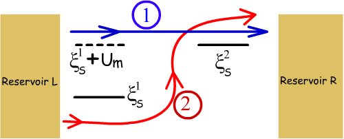
Figure 10: Schematic diagram depicting the two current components through the triple dot set-up. “Component 1” (directed blue arrow) flows without absorbing heat packets from the remote reservoir $G$ and only depends on the occupancy probability of the ground state of $G_{1}$. “Component 2” (directed red line) flows by absorbing heat packets from the reservoir $G$, and results in extraction of heat from the same.

In this aspect of refrigeration of the target reservoir $G$, the proposed triple dot set-up, on the other hand, offers a significant edge over the dual dot set-up. It should be noted that an electron flow in the triple dot set-up does not always demand the extraction of a heat packet from the reservoir $G$. To understand this, the components of current flow in the triple dot set-up are demonstrated in Fig. 10. As noted from Fig. 10, “Component 1” flows directly from reservoir $L$ to $R$, without absorbing heat packets from reservoir $G$. This component flows when the ground state of the dot $G_{1}$ is occupied. Hence, it depends mainly on the probability of occupancy of the dot $G_{1}$ and is not directly controlled by the parameter $\gamma_{g}$. “Component 2”, on the other hand, flows when the electron enters in the dot $S_{1}$ with unoccupied ground state of the dot $G_{1}$. Hence, this component flows by absorbing heat packets from reservoir $G$ and depends on the rate at which electrons can enter and exit the dot $G_{1}$ at energy $\xi_{g}+U_{m}$ and $\xi_{g}$ respectively. Thus, this component depends on $\gamma_{g}$ and can be suppressed substantially by reducing $\gamma_{g}$. Thus, on decreasing $\gamma_{g}$, the magnitude of the heat current from reservoir $G$ can be suppressed substantially.
As demonstrated in Fig. 9(a), the triple dot setup extracts much lower heat current from the reservoir $G$, while offering an enhanced sensitivity. In addition, the heat current can be suppressed by a large amount without much impact on the sensitivity by decreasing $\gamma_{g}$. This is clearly demonstrated in Fig. 9(a) and (b), where decreasing $\gamma_{g}$ by a factor of $10$ in the triple dot (TD) set-up decreases the maximum extracted heat current from $1.6$fW to $0.276$fW (by a factor of almost $5.8$), while keeping the sensitivity almost unchanged. Thus, a smart fabrication strategy in the triple dot set-up may be employed to prevent thermometry induced refrigeration and temperature drift of the remote target reservoir $G$.

IV Conclusions

To conclude, in this paper, I have proposed current based non-local thermometry as a robust and practical alternative to thermoelectric voltage based operation. Subsequently, I have investigated current based thermometry performance and regime of operation of the conventional dual dot set-up. Proceeding further, I have proposed a triple dot non-local thermometer which demonstrates a higher sensitivity while bypassing the need for unrealistic step-like system-to-reservoir coupling, in addition to providing robustness against fabrication induced variability in the Coulomb coupling energy. Furthermore, it was demonstrated that suitable fabrication strategy in the triple dot set-up aids in suppressing thermometry induced refrigeration (heat-up) and temperature drift in the remote target reservoir to a significant extent. Thus, the triple dot set-up hosts multitude of advantages that are necessary to deploy quantum non-local thermometers in practical applications. In this paper, I have mainly considered the limit of weak coupling which restricts electronic transport in the sequential tunneling regime and validates the use of quantum master equation for system analysis. It would, however, be interesting to investigate the impacts of cotunneling on the thermometer performance as the system is gradually tuned towards the strong coupling regime. In addition, an analysis on the impacts of electron-phonon interaction on the system performance would also constitute an interesting study. Other practical design strategies for non-local quantum thermometers is left for future investigation. Nevertheless, the triple dot design investigated in this paper can be employed to fabricate highly sensitive and robust non-local “sub-Kelvin” range thermometers.

Acknowledgments: Aniket Singha would like to thank financial support from Sponsored Research and Industrial Consultancy (IIT Kharagpur) via grant no. IIT/SRIC/EC/MWT/2019-20/162, Ministry of Human Resource Development (MHRD), Government of India via Grant No. STARS/APR2019/PS/566/FS under STARS scheme and Science and Engineering Research Board (SERB), Government of India via Grant No. SRG/2020/000593 under SRG scheme.

Appendix A Another equivalent triple dot set-up for efficient non-local thermometry

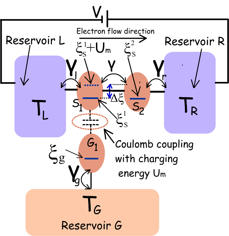
Figure 11: Schematic diagram for an equivalent triple dot design to accomplish efficient non-local thermometry. The thermometry performance of this set-up was found to be similar to the proposed triple dot set-up in Fig. 1(b) with a different regime of operation.

In this section, I show a variant of the triple dot set-up that can also be employed for efficient non-local thermometry in the regime of hundreds of “milli-Kelvin”. This set-up is demonstrated in Fig. 11 and is identical in construction to the set-up investigated in this paper (in Fig. 1.b). However, unlike the proposed set-up in Fig. 1(b), the ground-states of the two quantum dots $S_{1}$ and $S_{2}$ are aligned with each other, that is $\xi_{s}^{1}=\xi_{s}^{2}$. In this case, an electron tunneling from $G$ into $G_{1}$ misaligns the ground states in $S_{1}$ and $S_{2}$ and blocks the current flow through the system. A change in temperature of the reservoir $G$ impacts the probability of occupancy of $G_{1}$ and thus induces thermometry. Although not elaborated here, the configuration demonstrated in Fig. 11 demonstrates similar thermometry performance to the set-up shown in Fig. 1(b) with a different regime of operation. The configuration, demonstrated in Fig. 11, thus provides an alternative arrangement for efficient non-local thermometry.

Appendix B Derivation of quantum master equations (QME) for the triple dot thermometer

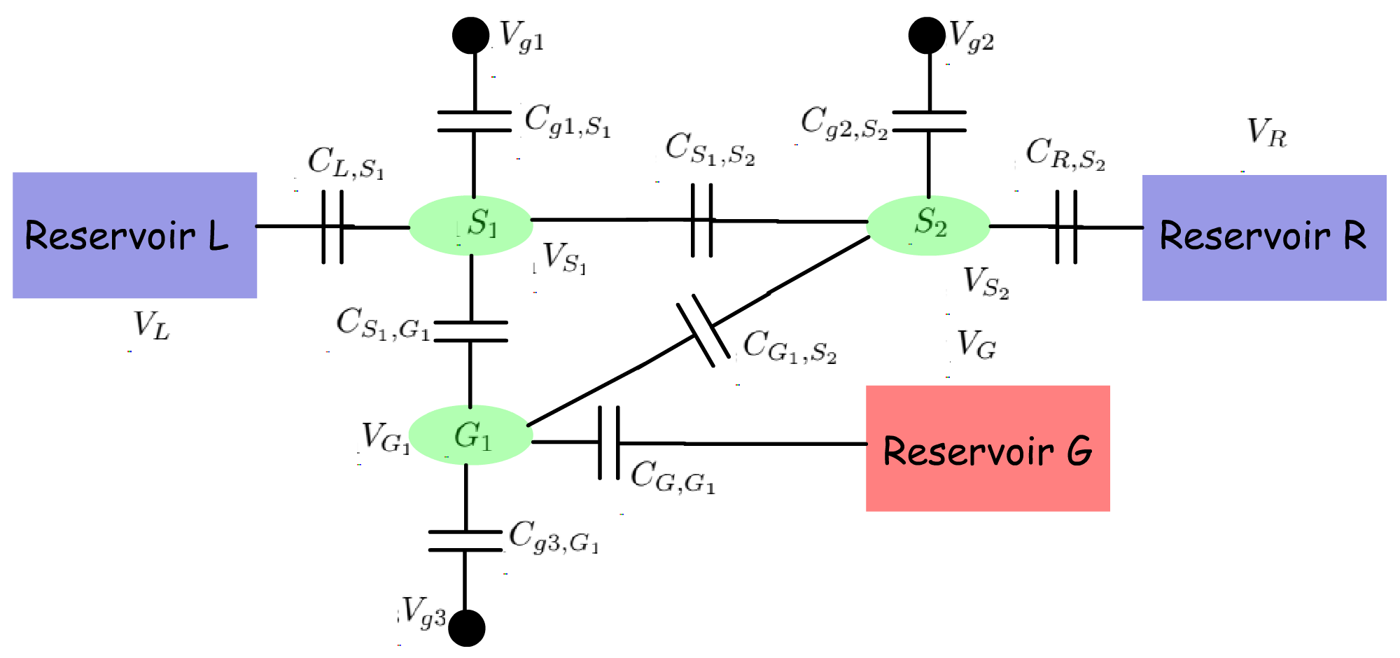
Figure 12: Schematic diagram demonstrating electrostatic interaction of the system with the adjacent electrodes and other dots. The voltages $V_{g1},~{}V_{g2},~{}V_{g3}$ are the voltages at the gate terminals of the dots $S_{1}$, $S_{2}$ and $G_{1}$ respectively.

In this section, I derive the quantum master equations (QME) for the proposed triple dot non-local thermometer, starting from the basic physics of Coulomb coupled systems. Fig. 12 depicts equivalent schematic model for electrostatic interaction of the quantum dots with the adjacent electrodes as well as the adjacent dots. $V_{g1},~{}V_{g2},~{}V_{g3}$ are the voltages at the gate terminals of the dots $S_{1}$, $S_{2}$ and $G_{1}$ respectively. The other symbols in Fig. 12 are self-explanatory. The potentials of the dots $S_{1},~{}S_{2}$ and $G_{1}$ can be calculated in terms of the quantum dot charge and the potentials at the adjacent terminals as cb :

$$V_{S_{1}}=\frac{Q_{S_{1}}}{C_{S_{1}}^{\Sigma}}+\frac{1}{C_{S_{1}}^{\Sigma}}\left\{C_{g1,S_{1}}V_{g1}+C_{L,S_{1}}V_{L}+C_{S_{1},S_{2}}V_{S_{2}}+C_{S_{1},G_{1}}V_{G_{1}}\right\}$$

$$V_{G_{1}}=\frac{Q_{G_{1}}}{C_{G_{1}}^{\Sigma}}+\frac{1}{C_{G_{1}}^{\Sigma}}\left\{C_{g3,G_{1}}V_{g3}+C_{G,G_{1}}V_{G}+C_{G_{1},S_{2}}V_{S_{2}}+C_{S_{1},G_{1}}V_{S_{1}}\right\}$$

$$V_{S_{2}}=\frac{Q_{S_{2}}}{C_{S_{2}}^{\Sigma}}+\frac{1}{C_{S_{2}}^{\Sigma}}\left\{C_{g2,S_{2}}V_{g2}+C_{R,S_{2}}V_{R}+C_{G_{1},S_{2}}V_{G_{1}}+C_{S_{1},S_{2}}V_{S_{1}}\right\},$$ (9)

where $Q_{x}$ is the charge in dot $x$ and the terms $C_{x}^{\Sigma}$ is the total capacitance seen by the dot $x$ with its adjacent environment.

$$C_{S_{1}}^{\Sigma}=C_{g1,S_{1}}+C_{S_{1},G_{1}}+C_{L,S_{1}}+C_{S_{1},S_{2}}$$

$$C_{S_{2}}^{\Sigma}=C_{g2,S_{2}}+C_{G_{1},S_{2}}+C_{R,S_{2}}+C_{S_{1},S_{2}}$$

$$C_{G_{1}}^{\Sigma}=C_{g3,G_{1}}+C_{S_{1},G_{1}}+C_{G,G_{1}}+C_{G_{1},S_{2}}$$ (10)

In general, each dot is coupled strongly with its corresponding gate terminal. Thus, from a practical purposes, the effective capacitance $C_{L,S_{1}},~{}C_{G,G_{1}}$ and $C_{R,S_{2}}$ between the quantum dots and the electrically-coupled electrodes can be neglected with respect to the gate coupling capacitances $C_{g1,S_{1}},~{}C_{g2,S_{2}}$ and $C_{g3,G_{1}}$. In addition, the dots $S_{1}$ and $G_{1}$ are strongly coupled (intentionally) by suitable fabrication techniques Hübel et al. [2007]; Chan et al. [2002]; Molenkamp et al. [1995]; Hübel et al. [2008]; Ruzin et al. [1992]. In addition, I assume that electrostatic coupling between $S_{1}-S_{2}$ and $G_{1}-S_{2}$ are negligible. However, $C_{S_{1},G_{1}}$ is enhanced via appropriate fabrication techniques Hübel et al. [2007]; Chan et al. [2002]; Molenkamp et al. [1995]; Hübel et al. [2008]; Ruzin et al. [1992], such that $C_{S_{1},G_{1}}>>(C_{S_{1},S_{2}},C_{G_{1},S_{2}})$. Hence, for the following derivations, I neglect the capacitances $C_{L,S_{1}},~{}C_{R,S_{2}},~{}C_{G,G_{1}},~{}C_{S_{1},S_{2}},~{}C_{G_{1},S_{2}}$. Under all these considerations, the total system electrostatic energy can be given by cb :

$$U_{tot}=\sum_{x\in(S_{1},S_{2},G_{1})}\frac{Q_{x}^{2}}{2C_{x}^{\Sigma}}+\frac{Q_{S_{1}}}{C^{\Sigma}_{S_{1}}}\left\{C_{g1,S_{1}}V_{g1}+C_{S_{1},G_{1}}V_{G_{1}}\right\}+\frac{Q_{S_{2}}}{C^{\Sigma}_{S_{2}}}C_{g2,S_{2}}V_{g2}+\frac{Q_{G_{1}}}{C^{\Sigma}_{G_{1}}}\left\{C_{g3,G_{1}}V_{g3}+C_{S_{1},G_{1}}V_{S_{1}}\right\},$$

where it is assumed that $C_{L,S_{1}},~{}C_{R,S_{2}},~{}C_{G,G_{1}},~{}C_{S_{1},S_{2}},~{}C_{G_{1},S_{2}}$ is negligible compared to the other capacitances in the system. At $0K$, the system would equilibriate at the minimum possible value of $U_{tot}$, which is termed as $U_{eq}$. The charge $Q_{S_{1}}^{eq}=-qn_{S_{1}}^{eq},~{}Q_{S_{2}}^{eq}=-qn_{S_{2}}^{eq}$ and $Q_{G_{1}}^{eq}=-qn_{G_{1}}^{eq}$ in the dot $S_{1},~{}S_{2}$ and $G_{1}$ respectively, in equilibrium (minimum energy condition) at $0K$, can be calculated by solving the set of equations given below:

$$\frac{\partial U_{tot}}{\partial Q_{S_{1}}}=\frac{Q_{S_{1}}}{C^{\Sigma}_{S_{1}}}+\frac{1}{C_{S_{1}}^{\Sigma}}(C_{g1,S_{1}}V_{g1}+C_{S_{1},G_{1}}V_{G_{1}})+\frac{(C_{S_{1},G_{1}})^{2}Q_{S_{1}}}{C_{G_{1}}^{\Sigma}(C_{S_{1}}^{\Sigma})^{2}}+\frac{C_{S_{1},G_{1}}Q_{G_{1}}}{C_{S_{1}}^{\Sigma}C_{G_{1}}^{\Sigma}}=0$$

$$\frac{\partial U_{tot}}{\partial Q_{S_{2}}}=\frac{Q_{S_{2}}}{C^{\Sigma}_{S_{2}}}+\frac{C_{g2,S_{2}}}{C_{S_{2}}^{\Sigma}}V_{g2}=0$$

$$\frac{\partial U_{tot}}{\partial Q_{G_{1}}}=\frac{Q_{G_{1}}}{C^{\Sigma}_{G_{1}}}+\frac{1}{C_{G_{1}}^{\Sigma}}(C_{g3,G_{1}}V_{g3}+C_{S_{1},G_{1}}V_{G_{3}})+\frac{(C_{S_{1},G_{1}})^{2}Q_{G_{1}}}{C_{S_{1}}^{\Sigma}(C_{G_{1}}^{\Sigma})^{2}}+\frac{C_{S_{1},G_{1}}Q_{S_{1}}}{C_{G_{1}}^{\Sigma}C_{S_{1}}^{\Sigma}}=0$$ (12)

The above set of equations can be derived by partial differentiation of Eq. LABEL:eq:utot, and replacing appropriate expressions obtained from partial differentiation and algebraic manipulation of the set of Eqns. LABEL:eq:potential. The number of electrons in the dots may vary stochastically due to application of external voltage bias or thermal fluctuations from the reservoir at finite temperature. The small increase in the net system electrostatic potential energy due to application of external bias or thermal fluctuations from the reservoirs can be given via a Taylor’s expansion of Eq. (LABEL:eq:utot) around the equilibrium dot charges ($-qn_{S_{1}}^{eq},~{}-qn_{S_{2}}^{eq}$ and $-qn_{G_{1}}^{eq}$), along with the condition $\frac{\partial U_{tot}}{\partial Q_{S_{1}}}\Big{|}_{Q_{S_{1}}=-qn_{S_{1}}^{eq}}=\frac{\partial U_{tot}}{\partial Q_{S_{2}}}\Big{|}_{Q_{S_{2}}=-qn_{S_{2}}^{eq}}=\frac{\partial U_{tot}}{\partial Q_{G_{1}}}\Big{|}_{Q_{G_{1}}=-qn_{G_{1}}^{eq}}=0$ as:

$$U(n_{S_{1}},n_{G_{1}},n_{S_{2}})=U_{tot}-U_{eq}=\sum_{x\in(S_{1},G_{1},S_{2})}\frac{q^{2}}{C^{self}_{x}}\left(n_{x}^{tot}-n_{x}^{eq}\right)^{2}+\sum_{(x_{1},x_{2})\in(S_{1},G_{1},S_{2})}^{x_{1}\neq x_{2}}U_{x_{1},x_{2}}\left(n_{x1}^{tot}-n_{x1}^{eq}\right)\left(n_{x2}^{tot}-n_{x2}^{eq}\right)$$

(13)

where $n_{x}^{tot}$ is the total number of electrons, and $C_{x}^{self}$ is self capacitance of the dot $x$. $U_{x_{1},x_{2}}$ denotes the electrostatic energy arising out of mutual Coulomb coupling between two different quantum dots, which accounts for a fluctuation in the electronic number of dot $x_{1(2)}$ affecting the electrostatic energy of dot $x_{2(1)}$. These quantities can be derived from the sets of Eqns. (LABEL:eq:potential), (LABEL:eq:utot) and (12), along with the assumption $C_{L,S_{1}}=C_{R,S_{2}}=C_{G,G_{1}}=C_{S_{1},S_{2}}=C_{G_{1},S_{2}}=0$ as:

$$\frac{1}{C_{S_{1}}^{self}}=\frac{\partial^{2}U_{tot}}{\partial Q_{S_{1}}^{2}}=\frac{1}{C_{S_{1}}^{\Sigma}}+2\frac{(C_{S_{1},G_{1}})^{2}}{(C_{S_{1}}^{\Sigma})^{2}C_{G_{1}}^{\Sigma}}$$

$$\frac{1}{C_{S_{2}}^{self}}=\frac{\partial^{2}U_{tot}}{\partial Q_{S_{2}}^{2}}=\frac{1}{C_{S_{2}}^{\Sigma}}$$

$$\frac{1}{C_{G_{1}}^{self}}=\frac{\partial^{2}U_{tot}}{\partial Q_{G_{1}}^{2}}=\frac{1}{C_{G_{1}}^{\Sigma}}+2\frac{(C_{S_{1},G_{1}})^{2}}{(C_{G_{1}}^{\Sigma})^{2}C_{S_{1}}^{\Sigma}}$$

$$\frac{U_{S_{1},G_{1}}}{q^{2}}=\frac{\partial^{2}U_{tot}}{\partial Q_{G_{1}}\partial Q_{S_{1}}}=\frac{\partial^{2}U_{tot}}{\partial Q_{S_{1}}\partial Q_{G_{1}}}=2\frac{C_{S_{1},G_{1}}}{C_{S_{1}}^{\Sigma}C_{G_{1}}^{\Sigma}}$$

$$\frac{U_{S_{1},S_{2}}}{q^{2}}=\frac{\partial^{2}U_{tot}}{\partial Q_{S_{1}}\partial Q_{S_{2}}}=\frac{\partial^{2}U_{tot}}{\partial Q_{S_{2}}\partial Q_{S_{1}}}=0$$

$$\frac{U_{S_{2},G_{1}}}{q^{2}}=\frac{\partial^{2}U_{tot}}{\partial Q_{G_{1}}\partial Q_{S_{2}}}=\frac{\partial^{2}U_{tot}}{\partial Q_{S_{2}}\partial Q_{G_{1}}}=0$$ (14)

From Eq. (13), I proceed to derive the QME of the entire system. In the triple dot set-up, the additional quantum dot $S_{2}$ is tunnel coupled to the $S_{1}$, while $G_{1}$ is Coulomb coupled to $S_{1}$. I assume that the electrostatic energy due to self-capacitance is much greater than the average thermal energy or the applied bias voltage, that is $E^{self}_{x}=\frac{q^{2}}{C^{self}_{x}}>>(kT,~{}qV)$, such that electronic transport through the Coulomb blocked energy level, due to self-capacitance, can be neglected. Thus the maximum number of electrons in the ground states of each quantum dots is limited to $1$. Under all these assumptions, the system analysis may be restricted to $2^{3}=8$ multi-electron states, that I indicate by the electron number in each quantum dot. Thus a state of interest in the system may be denoted by $\ket{n_{S_{1}},n_{G_{1}},n_{S_{2}}}=\ket{n_{S_{1}}}\mathbin{\mathop{\otimes}\limits}\ket{n_{G_{1}}}\mathbin{\mathop{\otimes}\limits}\ket{n_{S_{2}}}$, where $(n_{S_{1}},n_{G_{1}},n_{S_{2}})\in(0,1)$. To simplify these representations of multi-electron states, with a slight abuse of notation, I rename the states as $\ket{0,0,0}\rightarrow\ket{0}$, $\ket{0,0,1}\rightarrow\ket{1}$, $\ket{0,1,0}\rightarrow\ket{2}$, $\ket{0,1,1}\rightarrow\ket{3}$, $\ket{1,0,0}\rightarrow\ket{4}$, $\ket{1,0,1}\rightarrow\ket{5}$, $\ket{1,1,0}\rightarrow\ket{6}$, and $\ket{1,1,1}\rightarrow\ket{7}$
The simplified Hamiltonian of the triple dot system can hence be written as:

$$H=\sum_{\beta}\epsilon_{\beta}\ket{\beta}\bra{\beta}+t\{\ket{3}\bra{6}+\ket{1}\bra{4}\}$$

$$+U_{m}\{\ket{6}\bra{6}+\ket{7}\bra{7}\}+h.c.,$$ (15)

where $U_{m}=U^{m}_{S_{1},G_{1}}$ is the electrostatic coupling energy between $S_{1}$ and $G_{1}$ in Fig. 1, $t$ denotes the interdot tunnel coupling element or hopping parameter between $S_{1}$ and $S_{2}$ and $\epsilon_{\beta}$ is the total energy of the state $\ket{\beta}$ with respect to the vacuum state $\ket{0}$. Under the assumption that the interdot coupling element $t$ or the reservoir to dot coupling are small, the temporal dynamics of the system density matrix can be evaluated by taking the partial trace over the entire density matrix of the combined set-up consisting of the reservoirs and the dots Gurvitz [1998]; Hazelzet et al. [2001]; Dong et al. [2008, 2004]; Sztenkiel and Świrkowicz [2007]; Wegewijs and Nazarov [1999]. In this framework, the diagonal and the non-diagonal terms of the triple dot density matrix $\rho$ can be written as a set of modified Liouville equation Gurvitz [1998]; Hazelzet et al. [2001]; Dong et al. [2008, 2004]; Sztenkiel and Świrkowicz [2007]; Wegewijs and Nazarov [1999]:

$$\frac{\partial\rho_{\eta\eta}}{\partial t}=-i[H,\rho]_{\eta\eta}-\sum_{\nu}\Gamma_{\eta\nu}\rho_{\eta\eta}+\sum_{\delta}\Gamma_{\delta\eta}\rho_{\delta\delta}$$

$$\frac{\partial\rho_{\eta\beta}}{\partial t}=-i[H,\rho]_{\eta\beta}-\frac{1}{2}\sum_{\nu}\Big{(}\Gamma_{\eta\nu}+\Gamma_{\beta\nu}\Big{)}\rho_{\eta\beta},$$

(16)

where $\rho_{\eta\beta}=\bra{\eta}\rho\ket{\beta}$ and $[x,y]$ denotes the commutator of the operators $x$ and $y$. The terms $\rho_{\eta\eta}$ and $\rho_{\eta\beta}$ in the above equation represent diagonal and non-diagonal elements of the system density matrix respectively. The off-diagonal elements $\rho_{\eta\beta}$ account for coherent inter-dot tunneling, in addition to tunneling of electrons between the dots and the reservoirs. The off-diagonal terms $\rho_{\eta\beta}$, thus, are only non-zero and finite when electron tunneling can result in the transition between the states $\eta$ and $\beta$ or vice-versa. The parameters $\Gamma_{xy}$ account for the transition between system states due to electronic tunneling between the system and the reservoirs and are only finite when the system state transition from $\ket{x}$ to $\ket{y}$ (or vice-versa) is possible due to electron transfer between the system and the reservoirs. Assuming a statistical quasi-Fermi distribution inside the reservoirs, $\Gamma_{xy}$ can be given as:

$$\Gamma_{xy}=\gamma_{\lambda}f_{\lambda}(\epsilon_{y}-\epsilon_{x}),$$ (17)

where $f_{\lambda}(\epsilon)$ denotes the probability of occupancy of an electron in the corresponding reservoir $\lambda$ (driving the state transition) at energy $\epsilon$, $\epsilon_{x(y)}$ is the total electronic energy in the state $\ket{x(y)}$ compared to vacuum, and $\gamma_{\lambda}$ denotes the system to reservoir coupling for the corresponding reservoir $\lambda$.
For the triple dot set-up, tunneling of electrons between the quantum dots drives the system from $\ket{4}$ to $\ket{1}$ and from $\ket{3}$ to $\ket{6}$ (or vice-versa). In steady state, the time-derivative of each density matrix element $[\rho]$ vanishes. Hence, employing the second equation of (16), I get,

$$\rho_{4,1}=\rho^{*}_{1,4}=\frac{\rho_{4,4}-\rho_{1,1}}{\epsilon_{4}-\epsilon_{1}-i\frac{\Upsilon_{4,1}}{2}}$$ (18)

$$\rho_{6,3}=\rho^{*}_{3,6}=\frac{\rho_{6,6}-\rho_{3,3}}{\epsilon_{6}-\epsilon_{3}-i\frac{\Upsilon_{6,3}}{2}},$$ (19)

where $\Upsilon_{x,y}$ is the sum of net tunneling rates between the system and the reservoirs that leads to the decay of the states $\ket{x}$ and $\ket{y}$. In Eqns. (18) and (19), $\Upsilon_{4,1}$ and $\Upsilon_{6,3}$ are given by:

$$\Upsilon_{4,1}=\Gamma_{\ket{4},\ket{0}}+\Gamma_{\ket{4},\ket{6}}+\Gamma_{\ket{4},\ket{5}}+\Gamma_{\ket{1},\ket{0}}+\Gamma_{\ket{1},\ket{6}}+\Gamma_{\ket{1},\ket{3}}$$

$$\Upsilon_{6,3}=\Gamma_{\ket{6},\ket{4}}+\Gamma_{\ket{6},\ket{2}}+\Gamma_{\ket{6},\ket{7}}+\Gamma_{\ket{3},\ket{1}}+\Gamma_{\ket{3},\ket{2}}+\Gamma_{\ket{3},\ket{7}}$$ (20)

From Eq. (16), the time derivative of the density matrix elements $\rho_{6,6}$ and $\rho_{3,3}$ can be given by:

$$\dot{\rho}_{6,6}= it(\rho_{6,3}-\rho_{3,6})-\left(\Gamma_{\ket{6},\ket{4}}-\Gamma_{\ket{6},\ket{2}}+\Gamma_{\ket{6},\ket{7}}\right)\rho_{6,6}$$

$$+\Gamma_{\ket{4},\ket{6}}\rho_{4,4}+\Gamma_{\ket{2},\ket{6}}\rho_{2,2}+\Gamma_{\ket{7},\ket{6}}\rho_{7,7}$$

$$\dot{\rho}_{4,4}= it(\rho_{4,1}-\rho_{1,4})-\left(\Gamma_{\ket{4},\ket{0}}-\Gamma_{\ket{4},\ket{6}}+\Gamma_{\ket{4},\ket{5}}\right)\rho_{4,4}$$

$$+\Gamma_{\ket{0},\ket{4}}\rho_{0,0}+\Gamma_{\ket{6},\ket{4}}\rho_{6,6}+\Gamma_{\ket{5},\ket{4}}\rho_{5,5}$$

Substituting the values of $\rho_{6,3},~{}\rho_{3,6},~{}\rho_{4,1}$ and $\rho_{1,4}$ from Eq. (18) and (19) in Eq. (LABEL:eq:b8), time derivative of the probability of the states $\ket{4}$ and $\ket{6}$ can be given by:

$$\dot{p_{6}}=\dot{\rho}_{6,6}=\sum_{\alpha=}\left(-\Gamma_{\ket{6},\ket{\alpha}}p_{6}+\Gamma_{\ket{\alpha},\ket{6}}p_{\alpha}\right)$$

$$-\Lambda_{\ket{6},\ket{3}}p_{6}+\Lambda_{\ket{3},\ket{6}}p_{3}$$ (22)

$$\dot{p_{4}}=\dot{\rho}_{4,4}=\sum_{\alpha=}\left(-\Gamma_{\ket{4},\ket{\alpha}}p_{3}+\Gamma_{\ket{\alpha},\ket{4}}p_{\alpha}\right)$$

$$-\Lambda_{\ket{4},\ket{1}}p_{4}+\Lambda_{\ket{1},\ket{4}}p_{1},$$ (23)

where $p_{\eta}=\rho_{\eta,\eta}$ and

$$\Lambda_{\ket{6},\ket{3}}=\Lambda_{\ket{3},\ket{6}}=t^{2}\frac{\Upsilon_{6,3}}{(\epsilon_{6}-\epsilon_{3})^{2}+\frac{\Upsilon_{6,3}^{2}}{4}}$$

$$\Lambda_{\ket{4},\ket{1}}=\Lambda_{\ket{1},\ket{4}}=t^{2}\frac{\Upsilon_{4,1}}{(\epsilon_{4}-\epsilon_{1})^{2}+\frac{\Upsilon_{4,1}^{2}}{4}}$$

In Eq. LABEL:eq:tun_rate, $\Lambda_{\ket{4},\ket{1}}$ and $\Lambda_{\ket{6},\ket{3}}$ denote the rates of interdot tunneling between $S_{1}$ and $S_{2}$ with empty and occupied ground states of $G_{1}$ respectively. By a smart choice of the ground state energy positions, the condition $\epsilon_{6}=\xi_{g}+\xi_{s}^{1}+U_{m}=\xi_{g}+\xi_{s}^{2}=\epsilon_{3}$, that is $\xi_{s}^{2}=\xi_{s}^{1}+U_{m}$ is satisfied. In such a case, under the condition $U_{m}>>|\Upsilon_{4,1}|$, I get $\Lambda_{\ket{6},\ket{3}}>>\Lambda_{\ket{4},\ket{1}}$. This condition implies that the inter-dot tunneling probability between $S_{1}$ and $S_{2}$ is negligible when the ground state in $G_{1}$ is empty.
For the calculation of current, we need to know the probability of ground state in $S_{1}$ or $S_{2}$. Since, the electronic transport via the ground states in $S_{1}$ and $G_{1}$ are coupled to each other by Coulomb interaction, I consider $S_{1}$ and $G_{1}$ as a sub-system ($\varsigma_{1}$) of the total triple dot system. $S_{2}$ is considered to be the complementary sub-system ($\varsigma_{2}$) of the entire set-up. For the range of parameters used in this case, the condition $U_{m}>>|\Upsilon_{4,1}|$ is satisfied, which leads to $\Lambda_{\ket{4},\ket{1}}<<\Lambda_{\ket{6},\ket{3}}$. Hence, to simplify the calculations, I assume that $\Lambda_{\ket{4},\ket{1}}\approx 0$ all practical purposes relating to electron transport. In the following discussion, I simply denote $\Lambda_{\ket{6},\ket{3}}$ as $\gamma$ to represent the interdot tunnel coupling. I denote the occupancy probability of the subsystem $\varsigma_{1}$ as $P_{i,j}^{\varsigma_{1}}$, where $i$ and $j$ denote the electron number in the ground state of $S_{1}$ and $G_{1}$ respectively, while $P_{k}^{\varsigma_{2}}$ denotes the ground state occupancy probability of $S_{2}$. Note that splitting the entire system into two sub-systems in this fashion demands the limit of weak tunnel and Coulomb coupling between the two sub-systems such that the state of one sub-system remains unaffected by the state of the complementary sub-system. In such a limit, we can write $\rho_{0,0}=P^{\varsigma_{1}}_{0,0}P^{\varsigma_{2}}_{0},~{}\rho_{1,1}=P^{\varsigma_{1}}_{0,0}P^{\varsigma_{2}}_{1},~{}\rho_{2,2}=P^{\varsigma_{1}}_{0,1}P^{\varsigma_{2}}_{0},~{}\rho_{3,3}=P^{\varsigma_{1}}_{0,1}P^{\varsigma_{2}}_{1},~{}\rho_{4,4}=P^{\varsigma_{1}}_{1,0}P^{\varsigma_{2}}_{0},~{}\rho_{5,5}=P^{\varsigma_{1}}_{1,0}P^{\varsigma_{2}}_{1},~{}\rho_{6,6}=P^{\varsigma_{1}}_{1,1}P^{\varsigma_{2}}_{1},~{}\rho_{7,7}=P^{\varsigma_{1}}_{1,1}P^{\varsigma_{2}}_{1}$ The quantum master equations (QME) for the sub-system $\varsigma_{1}$ can be given in terms of two or more diagonal elements of the density matrix, in (16), as:

$$\frac{d}{dt}(P_{0,0}^{\varsigma_{1}})=\frac{d}{dt}\left(\rho_{0,0}+\rho_{1,1}\right)= -P_{0,0}^{\varsigma_{1}}\{\gamma_{l}f_{L}(\xi_{s}^{1})+\gamma_{g}f_{G}(\xi_{g})\}+\gamma_{g}P_{0,1}^{\varsigma_{1}}\{1-f_{G}(\xi_{g})\}+\gamma_{l}P_{1,0}^{\varsigma_{1}}\{1-f_{L}(\xi_{s}^{1})\}$$

$$\frac{d}{dt}(P_{1,0}^{\varsigma_{1}})=\frac{d}{dt}\left(\rho_{5,5}+\rho_{4,4}\right)= -P_{1,0}^{\varsigma_{1}}\left\{\gamma_{l}\left(1-f_{L}(\xi_{s}^{1})\right)+\gamma_{g}f_{G}(\xi_{g}+U_{m})\right\}+\gamma_{g}P_{1,1}^{\varsigma_{1}}\left\{1-f_{G}(\xi_{g}+U_{m})\right\}+\gamma_{g}P_{0,0}^{\varsigma_{1}}f_{L}(\xi_{s}^{1})$$

$$\frac{d}{dt}(P_{0,1}^{\varsigma_{1}})=\frac{d}{dt}\left(\rho_{2,2}+\rho_{3,3}\right)= -P_{0,1}^{\varsigma_{1}}\left\{\gamma_{g}\left(1-f_{g}(\xi_{g}^{1})\right)+\gamma_{l}f_{L}(\xi_{s}^{1}+U_{m})+{\gamma}P^{\varsigma_{2}}_{1}\right\}$$

$$+\gamma_{g}P_{0,0}^{\varsigma_{1}}f_{G}(\xi_{g})+P_{1,1}^{\varsigma_{1}}\left\{\gamma_{l}\left(1-f_{L}(\xi_{s}^{1}+U_{m})\right)+\gamma P^{\varsigma_{2}}_{0}\right\}$$

$$\frac{d}{dt}(P_{1,1}^{\varsigma_{1}})=\frac{d}{dt}\left(\rho_{7,7}+\rho_{6,6}\right)= -P_{1,1}^{\varsigma_{1}}\left\{\gamma_{g}\left(1-f_{g}(\xi_{g}^{1}+U_{m})\right)+\gamma_{l}\left(1-f_{L}(\xi_{s}^{1}+U_{m})\right)+\gamma P^{\varsigma_{2}}_{0}\right\}$$

$$+\gamma_{g}P_{1,0}^{\varsigma_{1}}f_{G}(\xi_{g}+U_{m})+P_{0,1}^{\varsigma_{1}}\left\{\gamma_{l}f_{L}(\xi_{s}^{1}+U_{m})+\gamma P^{\varsigma_{2}}_{1}\right\}$$

where $\gamma=\Lambda_{\ket{6},\ket{3}}=\Lambda_{\ket{3},\ket{6}}$ and $\Lambda_{\ket{4},\ket{1}}=\Lambda_{\ket{1},\ket{4}}=0$. I assume quasi Fermi-Dirac electron distribution at the reservoirs. Hence, corresponding to the reservoir $\lambda$, and $\lambda\in(L,R,G)$ $f_{\lambda}(\epsilon)=\left\{1+exp\left(\frac{\epsilon-\mu_{\lambda}}{kT_{\lambda}}\right)\right\}^{-1}$. Similarly, the QME of the sub-system $\varsigma_{2}$ can be written as:

$$\frac{d}{dt}(P_{0}^{\varsigma_{2}})=\frac{d}{dt}\left(\rho_{6,6}+\rho_{4,4}+\rho_{2,2}+\rho_{0,0}\right)=-P_{0}^{\varsigma_{2}}\{\gamma_{r}f_{R}(\xi_{s}^{2})+{\gamma}P_{1,1}^{\varsigma_{1}}\}+P_{1}^{\varsigma_{2}}\{\gamma_{r}\left(1-f_{R}(\xi_{s}^{2})\right)+{\gamma}P^{\varsigma_{1}}_{0,1}\}$$

$$\frac{d}{dt}(P_{1}^{\varsigma_{2}})=\frac{d}{dt}\left(\rho_{7,7}+\rho_{5,5}+\rho_{3,3}+\rho_{1,1}\right)=-P_{1}^{\varsigma_{2}}\{\gamma_{r}\left(1-f_{R}(\xi_{s}^{2})\right)+{\gamma}P^{\varsigma_{1}}_{0,1}\}+P_{0}^{\varsigma_{2}}\{\gamma_{r}f_{R}(\xi_{s}^{2})+{\gamma}P_{1,1}^{\varsigma_{1}}\}$$

The L.H.S of Eqns. (LABEL:eq:first_sys1) and (LABEL:eq:second_sys1) are zero in steady state. The set of Eqns. (LABEL:eq:first_sys1) and (LABEL:eq:second_sys1) form a coupled system of equations which were solved iteratively via Newton-Raphson method. On solution of the steady-state probabilities, the charge current $I_{L(R)}$ between reservoir $L$ and $R$ and the electronic heat current ($I_{Qe}$) extracted from the reservoir $G$ can be calculated by the equations:

$$I_{L}=q\gamma_{l}\times\left\{P^{\varsigma_{1}}_{0,0}f_{L}(\xi_{s}^{1})+P^{\varsigma_{1}}_{0,1}f_{L}(\xi_{s}^{1}+U_{m})-P^{\varsigma_{1}}_{1,0}\{1-f_{L}(\xi_{s}^{1})\}-P^{\varsigma_{s}^{1}}_{1,1}\{1-f_{L}(\xi_{s}^{1}+U_{m})\}\right\}$$ (27)

$$I_{R}=-q\gamma_{r}\times\left\{P^{\varsigma_{2}}_{0}f_{R}(\xi_{s}^{1})-P^{\varsigma_{2}}_{1}\{1-f_{R}(\xi_{s}^{1})\}\right\}$$ (28)

$$I_{Q}=\gamma_{g}\times\left\{(\xi_{g}+U_{m}-\mu_{g})\left\{P^{\varsigma_{1}}_{1,0}f_{G}(\xi_{g}+U_{m})-P^{\varsigma_{1}}_{1,1}\{1-f_{G}(\xi_{g}+U_{m})\}\right\}\right\}$$

$$+\gamma_{g}\times\left\{(\xi_{g}-\mu_{g})\times\left\{P^{\varsigma_{1}}_{0,0}f_{G}(\xi_{g})-P^{\varsigma_{n}}_{0,1}\{1-f_{G}(\xi_{g})\}\right\}\right\}$$ (29)

Since, net current into (out-of) the reservoir $G$ is zero, we have

$$I_{G}=q\gamma_{g}\times\left\{P^{\varsigma_{1}}_{1,0}f_{G}(\xi_{g}+U_{m})-P^{\varsigma_{1}}_{1,1}\{1-f_{G}(\xi_{g}+U_{m})\}+P^{\varsigma_{1}}_{0,0}f_{G}(\xi_{g})-P^{\varsigma_{n}}_{0,1}\{1-f_{G}(\xi_{g})\}\right\}=0$$ (30)

Substituting Eq. (30) in Eq. (29), I get

$$I_{Q}=\gamma_{g}\times U_{m}\left\{P^{\varsigma_{1}}_{1,0}f_{G}(\xi_{g}+U_{m})-P^{\varsigma_{1}}_{1,1}\{1-f_{G}(\xi_{g}+U_{m})\}\right\}$$ (31)

References

- Sothmann et al. [2014] B. Sothmann, R. Sánchez, and A. N. Jordan, Nanotechnology 26, 032001 (2014), URL https://doi.org/10.1088%2F0957-4484%2F26%2F3%2F032001.
- Singha [2020a] A. Singha, Journal of Applied Physics 127, 234903 (2020a), URL https://doi.org/10.1063/5.0007347.
- Benenti et al. [2017] G. Benenti, G. Casati, K. Saito, and R. S. Whitney, Physics Reports 694, 1 (2017), ISSN 0370-1573, fundamental aspects of steady-state conversion of heat to work at the nanoscale, URL http://www.sciencedirect.com/science/article/pii/S0370157317301540.
- Staring et al. [1993] A. A. M. Staring, L. W. Molenkamp, B. W. Alphenaar, H. van Houten, O. J. A. Buyk, M. A. A. Mabesoone, C. W. J. Beenakker, and C. T. Foxon, Europhysics Letters (EPL) 22, 57 (1993), URL https://doi.org/10.1209%2F0295-5075%2F22%2F1%2F011.
- Dzurak et al. [1993] A. Dzurak, C. Smith, M. Pepper, D. Ritchie, J. Frost, G. Jones, and D. Hasko, Solid State Communications 87, 1145 (1993), ISSN 0038-1098, URL http://www.sciencedirect.com/science/article/pii/0038109893908199.
- Humphrey et al. [2002] T. E. Humphrey, R. Newbury, R. P. Taylor, and H. Linke, Phys. Rev. Lett. 89, 116801 (2002), URL https://link.aps.org/doi/10.1103/PhysRevLett.89.116801.
- Entin-Wohlman et al. [2010] O. Entin-Wohlman, Y. Imry, and A. Aharony, Phys. Rev. B 82, 115314 (2010), URL https://link.aps.org/doi/10.1103/PhysRevB.82.115314.
- Sánchez and Büttiker [2011a] R. Sánchez and M. Büttiker, Phys. Rev. B 83, 085428 (2011a), URL https://link.aps.org/doi/10.1103/PhysRevB.83.085428.
- Singha et al. [2015] A. Singha, S. D. Mahanti, and B. Muralidharan, AIP Advances 5, 107210 (2015), URL http://scitation.aip.org/content/aip/journal/adva/5/10/10.1063/1.4933125.
- Sothmann et al. [2012a] B. Sothmann, R. Sánchez, A. N. Jordan, and M. Büttiker, Phys. Rev. B 85, 205301 (2012a), URL https://link.aps.org/doi/10.1103/PhysRevB.85.205301.
- De and Muralidharan [2018] B. De and B. Muralidharan, Scientific Reports 8, 5185 (2018), ISSN 2045-2322, URL https://doi.org/10.1038/s41598-018-23402-6.
- De and Muralidharan [2019] B. De and B. Muralidharan, Journal of Physics: Condensed Matter 32, 035305 (2019), URL https://doi.org/10.1088%2F1361-648x%2Fab3f82.
- De and Muralidharan [2016] B. De and B. Muralidharan, Phys. Rev. B 94, 165416 (2016), URL https://link.aps.org/doi/10.1103/PhysRevB.94.165416.
- Singha [2020b] A. Singha, Physica E: Low-dimensional Systems and Nanostructures 117, 113832 (2020b), ISSN 1386-9477, URL http://www.sciencedirect.com/science/article/pii/S1386947719313803.
- Singha and Muralidharan [2017] A. Singha and B. Muralidharan, Scientific Reports 7, 7879 (2017), ISSN 2045-2322, URL https://doi.org/10.1038/s41598-017-07935-w.
- Sothmann and Büttiker [2012] B. Sothmann and M. Büttiker, EPL (Europhysics Letters) 99, 27001 (2012), URL https://doi.org/10.1209%2F0295-5075%2F99%2F27001.
- Bergenfeldt et al. [2014] C. Bergenfeldt, P. Samuelsson, B. Sothmann, C. Flindt, and M. Büttiker, Phys. Rev. Lett. 112, 076803 (2014), URL https://link.aps.org/doi/10.1103/PhysRevLett.112.076803.
- Sánchez et al. [2015] R. Sánchez, B. Sothmann, and A. N. Jordan, Phys. Rev. Lett. 114, 146801 (2015), URL https://link.aps.org/doi/10.1103/PhysRevLett.114.146801.
- Hofer and Sothmann [2015] P. P. Hofer and B. Sothmann, Phys. Rev. B 91, 195406 (2015), URL https://link.aps.org/doi/10.1103/PhysRevB.91.195406.
- Roche et al. [2015a] B. Roche, P. Roulleau, T. Jullien, Y. Jompol, I. Farrer, D. A. Ritchie, and D. C. Glattli, Nature Communications 6, 6738 (2015a), ISSN 2041-1723, URL https://doi.org/10.1038/ncomms7738.
- Hartmann et al. [2015a] F. Hartmann, P. Pfeffer, S. Höfling, M. Kamp, and L. Worschech, Phys. Rev. Lett. 114, 146805 (2015a), URL https://link.aps.org/doi/10.1103/PhysRevLett.114.146805.
- Thierschmann et al. [2015a] H. Thierschmann, R. Sánchez, B. Sothmann, F. Arnold, C. Heyn, W. Hansen, H. Buhmann, and L. W. Molenkamp, Nature Nanotechnology 10, 854 (2015a), ISSN 1748-3395, URL https://doi.org/10.1038/nnano.2015.176.
- Whitney et al. [2016a] R. S. Whitney, R. Sánchez, F. Haupt, and J. Splettstoesser, Physica E: Low-dimensional Systems and Nanostructures 75, 257 (2016a), ISSN 1386-9477, URL http://www.sciencedirect.com/science/article/pii/S1386947715302083.
- Schulenborg et al. [2017] J. Schulenborg, A. Di Marco, J. Vanherck, M. Wegewijs, and J. Splettstoesser, Entropy 19, 668 (2017), ISSN 1099-4300, URL http://dx.doi.org/10.3390/e19120668.
- Josefsson et al. [2018] M. Josefsson, A. Svilans, A. M. Burke, E. A. Hoffmann, S. Fahlvik, C. Thelander, M. Leijnse, and H. Linke, Nature Nanotechnology 13, 920 (2018), ISSN 1748-3395, URL https://doi.org/10.1038/s41565-018-0200-5.
- Sánchez et al. [2019] R. Sánchez, J. Splettstoesser, and R. S. Whitney, Physical Review Letters 123 (2019), ISSN 1079-7114, URL http://dx.doi.org/10.1103/PhysRevLett.123.216801.
- Giazotto et al. [2006] F. Giazotto, T. T. Heikkilä, A. Luukanen, A. M. Savin, and J. P. Pekola, Rev. Mod. Phys. 78, 217 (2006), URL https://link.aps.org/doi/10.1103/RevModPhys.78.217.
- Pekola and Hekking [2007] J. P. Pekola and F. W. J. Hekking, Phys. Rev. Lett. 98, 210604 (2007), URL https://link.aps.org/doi/10.1103/PhysRevLett.98.210604.
- Singha [2018] A. Singha, Physics Letters A 382, 3026 (2018), ISSN 0375-9601, URL http://www.sciencedirect.com/science/article/pii/S0375960118307606.
- Singha and Muralidharan [2018] A. Singha and B. Muralidharan, Journal of Applied Physics 124, 144901 (2018), URL https://doi.org/10.1063/1.5044254.
- Edwards et al. [1993] H. L. Edwards, Q. Niu, and A. L. de Lozanne, Applied Physics Letters 63, 1815 (1993), eprint https://doi.org/10.1063/1.110672, URL https://doi.org/10.1063/1.110672.
- Prance et al. [2009] J. R. Prance, C. G. Smith, J. P. Griffiths, S. J. Chorley, D. Anderson, G. A. C. Jones, I. Farrer, and D. A. Ritchie, Phys. Rev. Lett. 102, 146602 (2009), URL https://link.aps.org/doi/10.1103/PhysRevLett.102.146602.
- Zhang et al. [2015a] Y. Zhang, G. Lin, and J. Chen, Phys. Rev. E 91, 052118 (2015a), URL https://link.aps.org/doi/10.1103/PhysRevE.91.052118.
- Koski et al. [2015a] J. V. Koski, A. Kutvonen, I. M. Khaymovich, T. Ala-Nissila, and J. P. Pekola, Phys. Rev. Lett. 115, 260602 (2015a), URL https://link.aps.org/doi/10.1103/PhysRevLett.115.260602.
- Mukherjee et al. [2020] S. Mukherjee, B. De, and B. Muralidharan, Three terminal vibron coupled hybrid quantum dot thermoelectric refrigeration (2020), eprint 2004.12763.
- Hofer et al. [2016] P. P. Hofer, M. Perarnau-Llobet, J. B. Brask, R. Silva, M. Huber, and N. Brunner, Phys. Rev. B 94, 235420 (2016), URL https://link.aps.org/doi/10.1103/PhysRevB.94.235420.
- Sánchez [2017a] R. Sánchez, Applied Physics Letters 111, 223103 (2017a), eprint https://doi.org/10.1063/1.5008481, URL https://doi.org/10.1063/1.5008481.
- Scheibner et al. [2008] R. Scheibner, M. König, D. Reuter, A. D. Wieck, C. Gould, H. Buhmann, and L. W. Molenkamp, New Journal of Physics 10, 083016 (2008), URL https://doi.org/10.1088%2F1367-2630%2F10%2F8%2F083016.
- Ruokola and Ojanen [2011] T. Ruokola and T. Ojanen, Phys. Rev. B 83, 241404 (2011), URL https://link.aps.org/doi/10.1103/PhysRevB.83.241404.
- Fornieri et al. [2014] A. Fornieri, M. J. Martínez-Pérez, and F. Giazotto, Applied Physics Letters 104, 183108 (2014), eprint https://doi.org/10.1063/1.4875917, URL https://doi.org/10.1063/1.4875917.
- Jiang et al. [2015a] J.-H. Jiang, M. Kulkarni, D. Segal, and Y. Imry, Phys. Rev. B 92, 045309 (2015a), URL https://link.aps.org/doi/10.1103/PhysRevB.92.045309.
- Sánchez et al. [2015] R. Sánchez, B. Sothmann, and A. N. Jordan, New Journal of Physics 17, 075006 (2015), URL https://doi.org/10.1088%2F1367-2630%2F17%2F7%2F075006.
- Martínez-Pérez et al. [2015] M. J. Martínez-Pérez, A. Fornieri, and F. Giazotto, Nature Nanotechnology 10, 303 (2015), ISSN 1748-3395, URL https://doi.org/10.1038/nnano.2015.11.
- Jiang et al. [2015b] J.-H. Jiang, M. Kulkarni, D. Segal, and Y. Imry, Phys. Rev. B 92, 045309 (2015b), URL https://link.aps.org/doi/10.1103/PhysRevB.92.045309.
- Li et al. [2006] B. Li, L. Wang, and G. Casati, Applied Physics Letters 88, 143501 (2006), eprint https://doi.org/10.1063/1.2191730, URL https://doi.org/10.1063/1.2191730.
- Joulain et al. [2016] K. Joulain, J. Drevillon, Y. Ezzahri, and J. Ordonez-Miranda, Phys. Rev. Lett. 116, 200601 (2016), URL https://link.aps.org/doi/10.1103/PhysRevLett.116.200601.
- Sánchez et al. [2017] R. Sánchez, H. Thierschmann, and L. W. Molenkamp, New Journal of Physics 19, 113040 (2017), URL https://doi.org/10.1088%2F1367-2630%2Faa8b94.
- Sánchez et al. [2017] R. Sánchez, H. Thierschmann, and L. W. Molenkamp, Phys. Rev. B 95, 241401 (2017), URL https://link.aps.org/doi/10.1103/PhysRevB.95.241401.
- Zhang et al. [2018] Y. Zhang, Z. Yang, X. Zhang, B. Lin, G. Lin, and J. Chen, EPL (Europhysics Letters) 122, 17002 (2018), URL https://doi.org/10.1209%2F0295-5075%2F122%2F17002.
- Tang et al. [2019] G. Tang, J. Peng, and J.-S. Wang, The European Physical Journal B 92, 27 (2019), ISSN 1434-6036, URL https://doi.org/10.1140/epjb/e2019-90747-0.
- Guo et al. [2018] B.-q. Guo, T. Liu, and C.-s. Yu, Phys. Rev. E 98, 022118 (2018), URL https://link.aps.org/doi/10.1103/PhysRevE.98.022118.
- Sánchez and Büttiker [2011b] R. Sánchez and M. Büttiker, Phys. Rev. B 83, 085428 (2011b), URL https://link.aps.org/doi/10.1103/PhysRevB.83.085428.
- Sothmann et al. [2012b] B. Sothmann, R. Sánchez, A. N. Jordan, and M. Büttiker, Phys. Rev. B 85, 205301 (2012b), URL https://link.aps.org/doi/10.1103/PhysRevB.85.205301.
- Roche et al. [2015b] B. Roche, P. Roulleau, T. Jullien, Y. Jompol, I. Farrer, D. A. Ritchie, and D. C. Glattli, Nature Communications 6, 6738 (2015b), ISSN 2041-1723, URL https://doi.org/10.1038/ncomms7738.
- Hartmann et al. [2015b] F. Hartmann, P. Pfeffer, S. Höfling, M. Kamp, and L. Worschech, Phys. Rev. Lett. 114, 146805 (2015b), URL https://link.aps.org/doi/10.1103/PhysRevLett.114.146805.
- Thierschmann et al. [2015b] H. Thierschmann, R. Sánchez, B. Sothmann, F. Arnold, C. Heyn, W. Hansen, H. Buhmann, and L. W. Molenkamp, Nature Nanotechnology 10, 854 (2015b), ISSN 1748-3395, URL https://doi.org/10.1038/nnano.2015.176.
- Whitney et al. [2016b] R. S. Whitney, R. Sánchez, F. Haupt, and J. Splettstoesser, Physica E: Low-dimensional Systems and Nanostructures 75, 257 (2016b), ISSN 1386-9477, URL http://www.sciencedirect.com/science/article/pii/S1386947715302083.
- Daré and Lombardo [2017] A.-M. Daré and P. Lombardo, Phys. Rev. B 96, 115414 (2017), URL https://link.aps.org/doi/10.1103/PhysRevB.96.115414.
- Walldorf et al. [2017] N. Walldorf, A.-P. Jauho, and K. Kaasbjerg, Phys. Rev. B 96, 115415 (2017), URL https://link.aps.org/doi/10.1103/PhysRevB.96.115415.
- Strasberg et al. [2018] P. Strasberg, G. Schaller, T. L. Schmidt, and M. Esposito, Phys. Rev. B 97, 205405 (2018), URL https://link.aps.org/doi/10.1103/PhysRevB.97.205405.
- Zhang et al. [2015b] Y. Zhang, G. Lin, and J. Chen, Phys. Rev. E 91, 052118 (2015b), URL https://link.aps.org/doi/10.1103/PhysRevE.91.052118.
- Koski et al. [2015b] J. V. Koski, A. Kutvonen, I. M. Khaymovich, T. Ala-Nissila, and J. P. Pekola, Phys. Rev. Lett. 115, 260602 (2015b), URL https://link.aps.org/doi/10.1103/PhysRevLett.115.260602.
- Sánchez [2017b] R. Sánchez, Applied Physics Letters 111, 223103 (2017b), eprint https://doi.org/10.1063/1.5008481, URL https://doi.org/10.1063/1.5008481.
- Erdman et al. [2018] P. A. Erdman, B. Bhandari, R. Fazio, J. P. Pekola, and F. Taddei, Phys. Rev. B 98, 045433 (2018), URL https://link.aps.org/doi/10.1103/PhysRevB.98.045433.
- Zhang and Chen [2019] Y. Zhang and J. Chen, Physica E: Low-dimensional Systems and Nanostructures 114, 113635 (2019), ISSN 1386-9477, URL http://www.sciencedirect.com/science/article/pii/S1386947719305818.
- Yang et al. [2019] J. Yang, C. Elouard, J. Splettstoesser, B. Sothmann, R. Sánchez, and A. N. Jordan, Phys. Rev. B 100, 045418 (2019), URL https://link.aps.org/doi/10.1103/PhysRevB.100.045418.
- Correa et al. [2015] L. A. Correa, M. Mehboudi, G. Adesso, and A. Sanpera, Phys. Rev. Lett. 114, 220405 (2015), URL https://link.aps.org/doi/10.1103/PhysRevLett.114.220405.
- Hofer et al. [2017] P. P. Hofer, J. B. Brask, M. Perarnau-Llobet, and N. Brunner, Phys. Rev. Lett. 119, 090603 (2017), URL https://link.aps.org/doi/10.1103/PhysRevLett.119.090603.
- Mehboudi et al. [2019] M. Mehboudi, A. Sanpera, and L. A. Correa, Journal of Physics A: Mathematical and Theoretical 52, 303001 (2019), URL https://doi.org/10.1088%2F1751-8121%2Fab2828.
- De Pasquale et al. [2016] A. De Pasquale, D. Rossini, R. Fazio, and V. Giovannetti, Nature communications 7, 12782 (2016), ISSN 2041-1723, 27681458[pmid], URL https://pubmed.ncbi.nlm.nih.gov/27681458.
- Spietz et al. [2003] L. Spietz, K. W. Lehnert, I. Siddiqi, and R. J. Schoelkopf, Science 300, 1929 (2003), ISSN 0036-8075, eprint https://science.sciencemag.org/content/300/5627/1929.full.pdf, URL https://science.sciencemag.org/content/300/5627/1929.
- Spietz et al. [2006] L. Spietz, R. J. Schoelkopf, and P. Pari, Applied Physics Letters 89, 183123 (2006), eprint https://doi.org/10.1063/1.2382736, URL https://doi.org/10.1063/1.2382736.
- Gasparinetti et al. [2011] S. Gasparinetti, F. Deon, G. Biasiol, L. Sorba, F. Beltram, and F. Giazotto, Phys. Rev. B 83, 201306 (2011), URL https://link.aps.org/doi/10.1103/PhysRevB.83.201306.
- Mavalankar et al. [2013] A. Mavalankar, S. J. Chorley, J. Griffiths, G. A. C. Jones, I. Farrer, D. A. Ritchie, and C. G. Smith, Applied Physics Letters 103, 133116 (2013), eprint https://doi.org/10.1063/1.4823703, URL https://doi.org/10.1063/1.4823703.
- Feshchenko et al. [2013] A. V. Feshchenko, M. Meschke, D. Gunnarsson, M. Prunnila, L. Roschier, J. S. Penttilä, and J. P. Pekola, Journal of Low Temperature Physics 173, 36 (2013), ISSN 1573-7357, URL https://doi.org/10.1007/s10909-013-0874-x.
- Maradan et al. [2014] D. Maradan, L. Casparis, T.-M. Liu, D. E. F. Biesinger, C. P. Scheller, D. M. Zumbühl, J. D. Zimmerman, and A. C. Gossard, Journal of Low Temperature Physics 175, 784 (2014), ISSN 1573-7357, URL https://doi.org/10.1007/s10909-014-1169-6.
- Feshchenko et al. [2015] A. V. Feshchenko, L. Casparis, I. M. Khaymovich, D. Maradan, O.-P. Saira, M. Palma, M. Meschke, J. P. Pekola, and D. M. Zumbühl, Phys. Rev. Applied 4, 034001 (2015), URL https://link.aps.org/doi/10.1103/PhysRevApplied.4.034001.
- Iftikhar et al. [2016] Z. Iftikhar, A. Anthore, S. Jezouin, F. D. Parmentier, Y. Jin, A. Cavanna, A. Ouerghi, U. Gennser, and F. Pierre, Nature Communications 7, 12908 (2016), ISSN 2041-1723, URL https://doi.org/10.1038/ncomms12908.
- Ahmed et al. [2018] I. Ahmed, A. Chatterjee, S. Barraud, J. J. L. Morton, J. A. Haigh, and M. F. Gonzalez-Zalba, Communications Physics 1, 66 (2018), ISSN 2399-3650, URL https://doi.org/10.1038/s42005-018-0066-8.
- Karimi and Pekola [2018] B. Karimi and J. P. Pekola, Phys. Rev. Applied 10, 054048 (2018), URL https://link.aps.org/doi/10.1103/PhysRevApplied.10.054048.
- Halbertal et al. [2016] D. Halbertal, J. Cuppens, M. B. Shalom, L. Embon, N. Shadmi, Y. Anahory, H. R. Naren, J. Sarkar, A. Uri, Y. Ronen, et al., Nature 539, 407 (2016), ISSN 1476-4687, URL https://doi.org/10.1038/nature19843.
- Hübel et al. [2007] A. Hübel, J. Weis, W. Dietsche, and K. v. Klitzing, Applied Physics Letters 91, 102101 (2007), URL https://doi.org/10.1063/1.2778542.
- Chan et al. [2002] I. H. Chan, R. M. Westervelt, K. D. Maranowski, and A. C. Gossard, Applied Physics Letters 80, 1818 (2002), URL https://doi.org/10.1063/1.1456552.
- Molenkamp et al. [1995] L. W. Molenkamp, K. Flensberg, and M. Kemerink, Phys. Rev. Lett. 75, 4282 (1995), URL https://link.aps.org/doi/10.1103/PhysRevLett.75.4282.
- Hübel et al. [2008] A. Hübel, K. Held, J. Weis, and K. v. Klitzing, Phys. Rev. Lett. 101, 186804 (2008).
- Ruzin et al. [1992] I. M. Ruzin, V. Chandrasekhar, E. I. Levin, and L. I. Glazman, Phys. Rev. B 45, 13469 (1992), URL https://link.aps.org/doi/10.1103/PhysRevB.45.13469.
- Eng et al. [2015] K. Eng, T. D. Ladd, A. Smith, M. G. Borselli, A. A. Kiselev, B. H. Fong, K. S. Holabird, T. M. Hazard, B. Huang, P. W. Deelman, et al., 1 (2015), URL https://advances.sciencemag.org/content/1/4/e1500214.
- Flentje et al. [2017] H. Flentje, B. Bertrand, P.-A. Mortemousque, V. Thiney, A. Ludwig, A. D. Wieck, C. Bäuerle, and T. Meunier, Applied Physics Letters 110, 233101 (2017), URL https://doi.org/10.1063/1.4984745.
- Froning et al. [2018] F. N. M. Froning, M. K. Rehmann, J. Ridderbos, M. Brauns, F. A. Zwanenburg, A. Li, E. P. A. M. Bakkers, D. M. Zumbühl, and F. R. Braakman, Applied Physics Letters 113, 073102 (2018), URL https://doi.org/10.1063/1.5042501.
- Noiri et al. [2017] A. Noiri, K. Kawasaki, T. Otsuka, T. Nakajima, J. Yoneda, S. Amaha, M. R. Delbecq, K. Takeda, G. Allison, A. Ludwig, et al., Semiconductor Science and Technology 32, 084004 (2017), URL https://doi.org/10.1088%2F1361-6641%2Faa7596.
- Hong et al. [2018] C. Hong, G. Yoo, J. Park, M.-K. Cho, Y. Chung, H.-S. Sim, D. Kim, H. Choi, V. Umansky, and D. Mahalu, Phys. Rev. B 97, 241115 (2018), URL https://link.aps.org/doi/10.1103/PhysRevB.97.241115.
- Takakura et al. [2014] T. Takakura, A. Noiri, T. Obata, T. Otsuka, J. Yoneda, K. Yoshida, and S. Tarucha, Applied Physics Letters 104, 113109 (2014), URL https://doi.org/10.1063/1.4869108.
- Datta [2005] S. Datta, Quantum Transport:Atom to Transistor (Cambridge Press, 2005).
- [94] Coulomb blockade in quantum dots, URL http://www.ftf.lth.se/fileadmin/ftf/Course_pages/FFF042/cb_lecture07.pdf.
- Gurvitz [1998] S. A. Gurvitz, Phys. Rev. B 57, 6602 (1998), URL https://link.aps.org/doi/10.1103/PhysRevB.57.6602.
- Hazelzet et al. [2001] B. L. Hazelzet, M. R. Wegewijs, T. H. Stoof, and Y. V. Nazarov, Phys. Rev. B 63, 165313 (2001), URL https://link.aps.org/doi/10.1103/PhysRevB.63.165313.
- Dong et al. [2008] B. Dong, X. L. Lei, and N. J. M. Horing, Phys. Rev. B 77, 085309 (2008), URL https://link.aps.org/doi/10.1103/PhysRevB.77.085309.
- Dong et al. [2004] B. Dong, H. L. Cui, and X. L. Lei, Phys. Rev. B 69, 035324 (2004), URL https://link.aps.org/doi/10.1103/PhysRevB.69.035324.
- Sztenkiel and Świrkowicz [2007] D. Sztenkiel and R. Świrkowicz, physica status solidi (b) 244, 2543 (2007), URL https://onlinelibrary.wiley.com/doi/abs/10.1002/pssb.200674623.
- Wegewijs and Nazarov [1999] M. R. Wegewijs and Y. V. Nazarov, Phys. Rev. B 60, 14318 (1999), URL https://link.aps.org/doi/10.1103/PhysRevB.60.14318.