How can scientists establish an observer-independent science?

Abstract

Embodied cognition posits that action and perception co-determine each other, forming an action-perception loop. This suggests that we humans somehow participate in what we perceive. So, how can scientists escape the action-perception loop to obtain an observer-independent description of the world? Here we model scientists engaged in the practice of science and argue that to achieve such a feat scientists must describe the world with the tools of quantum theory. This aligns with growing evidence suggesting that in quantum theory facts are relative. We argue that embodiment, as traditionally understood, can entail imaginary-time quantum dynamics. However, we argue that an embodied scientist interacting with an experimental system must be described from the perspective of another scientist, which is ignored in traditional approaches to embodied cognition. To describe the world without any reference to external observers we take two steps. First, we assume that observers play complementary roles as both objects experienced by other observers and “subjects” that experience other objects—here the word “subject” is used in a strict technical sense as the opposite of object. Second, like two mirrors reflecting each other as well as another object, we have to assume that two (sets of) observers mutually observe each other as well as the experimental system. This entails two coupled imaginary-time quantum dynamics that can be written as the imaginary and real parts of a genuine, real-time quantum dynamics. We discuss some potential implications of our work.

I Introduction

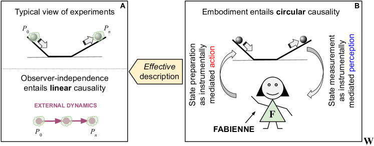
Figure 1: Effective seemingly observer-independent description of scientists doing experiments: (A) Experiments, and the world more generally, are typically viewed as observer-independent and so as instances of linear causality. (B) The instrumentally-mediated action-perception loop associated to an embodied scientist, Fabbiene (denoted by $F$), doing an experiment is usually considered an instance of circular causality. The circular causality of the instrumentally-mediated action-perception loop can indeed be effectively described in terms of a kind of linear causality (A)—the influence of the observer (green clouds) is effectively captured by describing the state of the system by a probability matrix that follows an imaginary-time quantum dynamics. However, here Fabbiene is described from the perspective of an external observer, Wigner (denoted by $W$—bottom right). Taking into account such an external observer can entail genuine real-time quantum dynamics.

A central theme in modern cognitive science is the idea that action and perception are circularly related and fundamentally inseparable varela2017embodied ; thompson2010mind ; di2017sensorimotor ; shapiro2019embodied ; djebbara2019sensorimotor ; wilson2002six ; bridgeman2011embodied . That is, action and perception co-determine each other, forming an action-perception loop—i.e., “a cycle in which perception leads to particular actions, which in turn create new perceptions, which then lead to new actions, and so on” shapiro2019embodied . Djebbara et al. djebbara2019sensorimotor recently reported experimental evidence for the existence of the action-perception loop. The idea that action and perception are somehow co-dependent has roots in a variety of fields wilson2002six , including Piaget’s developmental psychology, which holds that cognitive abilities somehow emerge from sensorimotor skills; Gibson’s ecological psychology, which sees perception in terms of potential interactions with the environment; and Merleau-Ponty’s phenomenology, which views perception not as something that happens inside an organism that passively receives information about the world, but as a process wherein the organism actively seeks out information and interprets it in terms of the bodily actions it enables.

The action-perception loop has been particularly emphasized in the research program of embodied cognition varela2017embodied ; thompson2010mind ; di2017sensorimotor ; shapiro2019embodied ; djebbara2019sensorimotor ; wilson2002six ; bridgeman2011embodied , which arose as a reaction against the view that “the mind and the world could be treated as separate and independent of each other, with the outside world mirrored by a representational model inside the head” thompson2010mind . In the traditional view, cognition begins with an input to the brain and ends with an output from the brain; so, traditional cognitive science can limit its investigations to processes within the head, without regard for the world outside the organism shapiro2019embodied .

In contrast, embodied cognition posits that “cognitive processes emerge from the nonlinear and circular causality of continuous sensorimotor interactions involving the brain, body, and environment” thompson2010mind In this view, perception does not result from passively sensing the physical world but from actively engaging with it in an ongoing reciprocal interaction between brain, body and world—such interactions could in principle be mediated by technologies that enhance motor and sensory capabilities. Again, we are involved in an action-perception loop, wherein we act to perceive and vice versa.

According to Varela et al. varela2017embodied , the overall concern of embodied cognition is “not to determine how some perceiver-independent world is to be recovered; it is, rather, to determine the common principles or lawful linkages between sensory and motor systems that explain how action can be perceptually guided in a perceiver-dependent world.” Along the same lines, more recently di Paolo et al. di2017sensorimotor say (comments within brackets are our own):

“Action in the world is always perceptually guided. And perception is always an active engagement with the world. The situated perceiver does not aim at extracting properties of the world as if these were pregiven, but at understanding the engagement of her body [possibly enhanced by technological devices] with her surroundings, usually in an attempt to bring about a desired change in relation between the two. To understand perception is to understand how these sensorimotor regularities or contingencies are generated by the coupling of body and world [possibly mediated by technologies that can enhance motor and sensory capabilities] and how they are used in the constitution of perceptual and perceptually guided acts.”

The action-perception loop is also emphasized in the theory of active inference, wherein an agent has a generative model of the external world and its motor systems suppress prediction errors through a dynamic interchange of prediction and action. In other words, “there are two ways to minimize prediction errors: to adjust predictions to fit the current sensory input and to adapt the unfolding of movement to make predictions come true. This is a unifying perspective on perception and action suggesting that action is both perceived by and caused by perception” djebbara2019sensorimotor .

According to Friston friston2013life , in active inference there is a circular causality analogous to the action-perception loop. Such circular causality means that “external states cause changes in internal states, via sensory states, while the internal states couple back to the external states through active states—such that internal and external states cause each other in a reciprocal fashion. This circular causality may be a fundamental and ubiquitous causal architecture for self-organization.”

While the research program of embodied cognition and related fields encompass a broad spectrum of views, among which there is still ongoing debate, we here focus only on the action-perception loop, which appears to be a rather uncontroversial feature. Moreover, as already mentioned, Djebbara et al. recently reported experimental evidence for the existence of the action-perception loop. Depending on the context and on the interest of the authors, the action-perception loop tends to be modeled with different tools and with different degrees of complexity. For instance, the enactive view of embodied cognition tends to emphasize dynamical systems, while active inference tends to emphasize variational Bayesian methods. Here we use tools from statistical physics to model the action-perception loop in a rather parsimonious way, focusing exclusively on its main feature: the circular causality between action and perception.

Now, in cognitive science it is routine to model human beings interacting with external systems. Here we investigate the particular case where the human beings are scientists and the external systems are experimental systems. That is, we model scientists performing scientific experiments. This reflexive application of science to itself brings up an interesting question. Indeed, the action-perception loop entails that humans play an active and constructive role in the information they perceive about the world. In contrast, scientists apparently manage to obtain a completely observer-independent view of the world, passively mirroring an external reality without influencing it in any way (see Fig. 1A). How do scientists achieve such a feat? Of course, technology enhances scientists’ capacities for perception and action, enabling them to transcend the limitations of their senses and to implement sophisticated interventions, e.g., at the sub-atomic level. However, while it is clear that technology can enable an enhanced, instrumentally-mediated action-perception loop, it is not at all clear that it can also change its circular topology. In other words, it is not clear that technology can break such an enhanced loop of instrumentally-mediated action and instrumentally-mediated perception (see Fig. 1B).

In brief, our approach allows us to ask: How can scientists establish an observer-independent science, even though this seems to defy the very notion of embodied cognition? In other words, how can scientists escape the action-perception loop? Of course, logical reasoning is another powerful tool that allows scientists to transcend their limitations. However, logical reasoning should be able to acknowledge the existence of the action-perception loop, if it exists, and tell us how is it that we escape it. From a different perspective, our approach could also be considered as a self-consistency check to materialism: instead of a priori neglecting the physics or embodiment of scientists, as if they were immaterial, we let a scientific analysis tells us a posteriori how is it that we can do so.

In principle, scientists differ from generic human beings in that they strive to achieve objectivity, which is often equated with observer-independence. Of course, we cannot start from the assumption of an observer-independent science since how this is established is precisely what we want to explore. Instead, we will use three conditions that, according to Velmans, characterize what in practice we may call a reliable science. These are velmans2009understanding (p. 219; see also Refs. varela2017embodied ; thompson2014waking ; bitbol2008consciousness ):

R1. Standardization: The procedures we used to investigate the world are standardized and explicit, so we clearly know what we are talking about.

R2. Intersubjectivity: The observations we do are intersubjective and repeatable, so we can mutually agree about the actual scientific facts.

R3. Truthfulness: Observers are dispassionate, accurate and truthful, for obvious reasons.

Again, we are not a priori equating the notion of reliability with that of objectivity in the sense of observer-independence. However this does not deny a priori either that an observer-independent science can be established. Indeed, the dynamics of our model is formally analogous to quantum dynamics. So, our approach is consistent with current scientific knowledge and could suggest a potential reconstruction of quantum theory Rovelli-1996 ; d2017quantum . Unlike current reconstructions, though, instead of working with an abstract notion of observer, our approach builds on general insights gained from the scientific investigation of actual observers—however, it is not necessarily restricted to a specific kind of them.

This work is outlined as follows. In Sec. II we discuss the circular dynamics of an embodied scientist interacting with an experimental system, which is similar to that of an action-perception loop friston2010free ; djebbara2019sensorimotor ; di2017sensorimotor . We show that this can entail a dynamics formally analogous to “imaginary-time” quantum dynamics. This is described by an Schrödinger’s equation without imaginary unit. While this is real-valued, genuine or “real-time” quantum dynamics is complex-valued. Somewhat analogous to RQM, in Sec. III we assume that a classical embodied scientist interacting with a classical experimental system must be described from the perspective of another scientist, which is ignored in traditional approaches to embodied cognition ($W$ in Fig. 1B). However, to be consistent we should also take into account who observes this new scientist. We escape the infinite regress that a naïve approach would entail in two steps. First, we assume that observers play complementary roles as both objects experienced by other observers and “subjects” that experience other objects. Here the word “subject” is used in a strict technical sense as the opposite of object. Second, like two mirrors reflecting each other as well as another object, we have to assume that two (sets of) observers mutually observe each other as well as the experimental system. This entails two coupled imaginary-time quantum dynamics that can be written as the imaginary and real parts of a genuine, real-time quantum dynamics. Finally, in Sec. IV we discuss some potential implications of our work.

II Embodiment and imaginary-time quantum dynamics

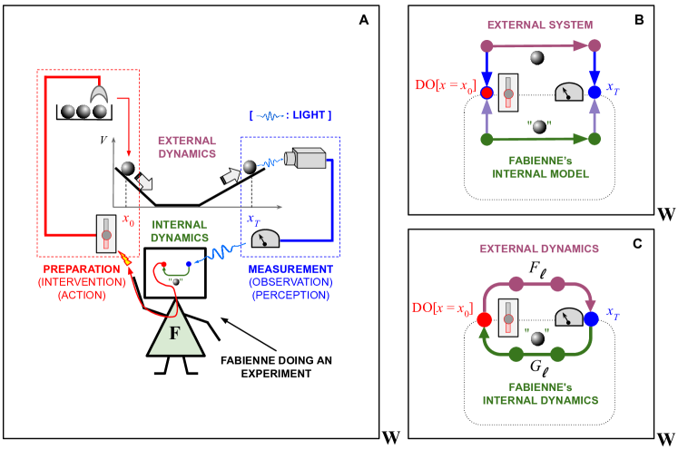
Figure 2: Experiments as circular processes: (A) A scientist (Fabbiene) doing an experiment. (B) Model of a scientist doing an experiment in the spirit of active inference. Fabbiene’s actions can always prepare the same initial state, $x=x_{0}$, effectively implementing a causal intervention (this is denoted here as $\textsc{do}[x=x0]$) (C) Enactive model of a scientist and an experimental system as two physical systems involved in a circular interaction (see Appendix B.2 and Fig. 10 therein). Arrows indicate the direction of the circular interaction, not conditional probabilities as in Bayesian networks. The internal factors, $G_{\ell}=F_{2n-1-\ell}$, can be considered as Fabienne’s physical correlates of the external factors, $F_{\ell}$—here $\ell=0,\dotsc,n$.

II.1 Embodied scientists doing experiments

Here we build on enactivism whose task is “to determine the common principles or lawful linkages between sensory and motor systems that explain how action can be perceptually guided in a perceiver-dependent world” varela2017embodied (p. 173) In Appendix B we provide a brief introduction to some aspects of embodied cognition.

Importantly, we neglect the long and painful learning stage, when scientists are engaged in the invention and fine-tuning of new protocols, devices, and even concepts (e.g., spacetime curvature) that enables them to couple to the world in ways that were not possible before, and thus to enact new kinds of lawful regularities. For instance, the kind of regularities associated to quantum and relativity theories, which are invisible to the naked eye, are enabled by sophisticated experimental protocols and devices, as well as conceptual frameworks, all developed by scientists themselves.

Figure 2A illustrates the dynamical coupling between an embodied scientist and an experimental system. This can be divided into four stages: (i) scientist’s interventions on the experimental system, e.g. via moving some knobs, for preparing the desired initial state—this requires the physical interaction between the knobs and the observer’s actuators; (ii) experimental system’s dynamics—this is the main process traditionally analyzed in physics; (iii) scientist’s measurement of the experimental system—this requires the physical interaction between the experimental system and the observer’s sensors via the measuring device; (iv) scientist’s internal dynamics which correlate with her experience of the experimental system.

In the related approach of active inference friston2010free ; schwobel2018active , experimental systems would be considered as generative processes which scientists can only access indirectly via the data generated in their sensorium (see Appendix B.1). Scientists can perturb such generative processes via their actions and have a generative model of their dynamics, including the effect of their own actions, which they can make as accurate as possible via learning. This is reflected in that, in Fig. 2B, the topology of the Bayesian network representing the scientist mirrors the topology of the Bayesian network representing the experimental system. In particular, both internal and external dynamics flow in the same direction (horizontal arrows in Fig. 2B; see Appendix B.1 and Fig. 9 therein).

Following enactivism varela2017embodied ; thompson2010mind ; di2017sensorimotor , instead, we give more relevance to the dynamical coupling between scientists and experimental systems. Learning scientific lawful regularities is not so much about extracting pre-existent properties of the world as about stabilizing this circular coupling and achieving “reliability” (conditions R1-R3 above). This may include the development of new technologies, protocols and concepts. The lawful regularities achieved in the post-learning stage are our focus here. So, our approach is independent of a specific theory of learning (see Fig. 2C; see also Appendix B.2 and Fig. 10 therein).

II.2 As simple as possible, but not simpler

Of course, the scientific process generally involves many scientists and technologies. However, much as the theory of relativity can be developed without modeling all types of realistic clocks, our approach aims at capturing some general underlying principles valid beyond the particular model investigated. For instance, we could also have a situation where, say, a scientist in the UK prepares a laser pulse to send to another scientist in the Netherlands who would then perform a measurement and send the result back to the former via email. Only after both scientists have communicated can they reach any scientific conclusions about any potential correlations between the initial and final states of the laser pulse. This would again be a circular process. Instead of two scientists we could have many and the fundamental process would still be circular. For simplicity, we focus here on a single scientist. However, experiments generally comprise the four stages above. So, ours can be considered as a model of a generic process of “reliable” observations—though ignoring relativistic considerations. This process is embodied because all scientists and technologies involved are so.

II.3 Experiments as circular processes

Here we setup the mathematical framework. Science is fundamentally concerned with causation, not with mere correlation. So, in general, a scientist do not passively observe the system to determine its initial state. Rather, she actively intervenes it to prepare a fixed initial state, runs the experiment and observes the final state. She repeats this enough times to determine the probability that, given that the initial state prepared is $x=x_{0}$, the final state observed is $x_{n}$. Using Pearl’s do-calculus, this probability can be denoted as $\overline{\mathcal{P}}(x_{n}|\textsc{do}[x=x_{0}])$, where $\textsc{do}[x=x_{0}]$ refers to the scientist’s intervention (notice the bar on $\overline{\mathcal{P}}$). Ideally, the scientist would prepare every possible initial state to compute the full probability distribution for any initial state, $x_{0}$ prepared—in practice this might be impossible, though. In principle, she can select each intervention with a given probability.

Unlike Pearl’s do-calculus, we explicitly model the scientist doing the causal intervention. So, instead of using the do operator, we can deal with such an intervention in a more direct manner, as we are about to see. As we mentioned earlier, we are considering only the post-learning stage, when the scientist is just repeating the experiment a statistically significant number of times. We model this as the stationary state, $\widetilde{\mathcal{P}}(\widetilde{\boldsymbol{x}})$, of a stochastic process on a cycle, which includes deterministic systems as a particular case (see Fig. 2C; notice the tildes on $\widetilde{\mathcal{P}}$ and $\widetilde{\boldsymbol{x}}$)—this allows us to establish a posteriori which is the case. Here $\widetilde{\mathbf{x}}=(x_{0},\dotsc,x_{k-1})$ denotes a closed path $x_{0}\to x_{1}\to\cdots\to x_{k-1}\to x_{0}$ which returns to $x_{k}=x_{0}$ due to the scientist’s causal interventions—as we said, experiments are not mere passive observations. This path could be divided into two open paths $x_{0}\to\cdots\to x_{n}$ and $x_{n}\to\cdots\to x_{k}$, with $x_{k}=x_{0}$, corresponding to the experimental system and the scientist, respectively. Furthermore, $\widetilde{\mathcal{P}}(\widetilde{\boldsymbol{x}})$ denotes the probability to observe a path $\widetilde{\mathbf{x}}$. As we said above, the scientist can in principle select each intervention with a given probability, so $\widetilde{\mathcal{P}}(\widetilde{\boldsymbol{x}})$ can be non-zero for paths with different values of $x_{0}$—again, causal interventions are reflected in the fact that paths are closed.

Since energy plays a key role in physics, we assume that the stationary state is characterized by an “energy” function $\mathcal{H}_{\ell}(x_{\ell+1},x_{\ell})$, where $0\leq\ell\leq k$ denotes the time step. For the case of a particle in a non-relativistic potential $V$ we have

$$\mathcal{H}_{\ell}(x_{\ell+1},x_{\ell})=\frac{m}{2}\left(\frac{x_{\ell+1}-x_{\ell}}{\epsilon}\right)^{2}+\frac{1}{2}\left[V(x_{\ell})+V(x_{\ell+1})\right].$$ (1)

for the external path ($\ell=0,\dotsc,n-1$)—in principle, the internal path ($\ell=n,\dotsc,k$) can have a different functional form (but see below). Unlike the traditional Hamiltonian function, $\mathcal{H}_{\ell}$ is written in terms of consecutive position variables, $x_{\ell}$ and $x_{\ell+1}$, rather than instantaneous position and momentum. The potential $V$ in Eq. (1) is symmetrized for convenience. We will discuss later on the case of more general, complex-valued, and so “non-stoquastic” Hamiltonians (see Sec. III.4.2 and Appendix A).

We derive $\widetilde{\mathcal{P}}$ using the principle of maximum path entropy presse2013principles , a general variational principle analogous to the free energy principle from which a wide variety of well-known stochastic models at, near, and far from equilibrium has been derived presse2013principles (see Appendix C.1). To do so, we use the assumption, common in statistical physics, that we only know the average energy on the cycle $E_{\rm av}=\left\langle\frac{\epsilon}{T}\sum_{\ell}\mathcal{H}_{\ell}\right\rangle_{\widetilde{\mathcal{P}}}$ (see below). Here $\epsilon\to 0$ is the time step size and $T=(k+1)\epsilon$ is the total duration of a cycle. This is known presse2013principles to yield a Boltzmann distribution (see Appendix C.1)

$$\widetilde{\mathcal{P}}\propto\exp\{-\epsilon\sum_{\ell}\mathcal{H}_{\ell}/{\Gamma}\},$$ (2)

where ${\Gamma}=T/\lambda$ and $\lambda$ is a Lagrange multiplier fixing the average energy $E_{\rm av}$ on the cycle (see Appendix C.1). We will investigate later on the potential sources of fluctuations characterized here by the temperature- or diffusion-like parameter $\Gamma$.

So, how can scientists escape their embodiment and obtain an observer-independent description of the world? Obviously, we cannot just forcefully neglect the scientist at this point. The proper way to ignore the scientist in our approach is by marginalizing $\widetilde{\mathcal{P}}$ over the degrees of freedom associated to her. So, following the tradition in physics, we now focus on the external system and ignore the scientist by marginalizing $\widetilde{\mathcal{P}}$ over the internal paths, i.e., over $(x_{n+1},\dotsc,x_{k-1})$. This yields (see Appendix C.1; notice the absence of tildes in the left-hand side)

$$\begin{split}\mathcal{P}(\mathbf{x})&=\sum_{x_{n+1},\dotsc,x_{k-1}}\widetilde{\mathcal{P}}(\widetilde{\mathbf{x}})\\ &=\frac{1}{Z}\widetilde{F}_{n}(x_{0}^{\prime},x_{n})\cdots F_{1}(x_{2},x_{1})F_{0}(x_{1},x_{0}),\end{split}$$ (3)

where $Z$ is the normalization constant and we have written $x_{0}^{\prime}=x_{0}$ for future convenience—here we use sums to indicate either sums or integrals depending on the context. The expression $\mathbf{x}=(x_{0},\dotsc,x_{n})$ denotes a path $x_{0}\to x_{1}\to\cdots\to x_{n}\to x_{0}$ which returns to $x_{0}$, but where we disregard how it does so. Furthermore,

$$\widetilde{F}_{n}(x_{0}^{\prime},x_{n})=\sum_{x_{n+1},\dotsc,x_{k-1}}F_{k-1}(x_{0}^{\prime},x_{k-1})\cdots F_{n}(x_{n+1},x_{n}),$$ (4)

summarizes the dynamics internal to the scientist, whose details we have disregarded, and

$$F_{\ell}(x^{\prime},x)=e^{-\epsilon\mathcal{H}_{\ell}(x^{\prime},x)/{\Gamma}}/Z_{\epsilon},$$ (5)

for $\ell=0,\dotsc,k$, where the constant $Z_{\epsilon}=\sqrt{2\pi\Gamma\epsilon/m}$ is introduced for convenience.

II.4 Circular causality and imaginary-time quantum dynamics

We now describe the relationship between our model of embodied scientists doing experiments (see Fig. 1B) and the typical view of experiments, and the world more generally (see Fig. 1A). We typically think of experiments and the world in terms of linear causality. That is, as external systems that have an observer-independent initial state that evolves forward in time according to some observer-independent dynamical law (see Fig. 1A). In contrast, the action-perception loop associated to an embodied scientist doing experiments is usually considered as an instance of circular causality (see Fig. 1B). Here we show that such a circular causality can be effectively described in terms of a kind of linear causality. That is, we will show that the circular dynamics entailed by the presence of the embodied scientist can be effectively described as if it were an observer-independent dynamics. The price to pay, however, is that the state of the system has to be described in terms of a probability matrix that follows a dynamics formally analogous to imaginary-time quantum dynamics (see Fig. 1).

II.4.1 Linear causality and Markov chains

First, notice that if we neglect the scientist, i.e., if we neglect the “energy” function associated to the internal paths, then $\widetilde{F}_{n}(x_{0},x_{n})$ becomes a constant. In this case the cycle in Fig. 2C turns into a chain and we recover the most parsimonious non-trivial dynamical model where the probability distribution in Eq. (3) is Markov with respect to a chain on variables $x_{\ell}$ pearl2009causality (p. 16; see Appendix C.2 herein)—a more parsimonious dynamical model would be memoryless.

In particular, by knowing only the initial marginal $p_{0}$ and the forward transition probabilities $\mathcal{P}_{\ell}^{+}$ from time step $\ell$ to $\ell+1$, for all $\ell$, we can readily obtain the probability for a path

$$\mathcal{P}_{\rm ch}(\mathbf{x})=p_{0}(x_{0})\mathcal{P}^{+}_{0}(x_{1}|x_{0})\cdots\mathcal{P}^{+}_{n-1}(x_{n}|x_{n-1}).$$ (6)

This implies in particular that we can obtain the marginal $p_{\ell+1}$ from the previous marginal $p_{\ell}$ via a Markovian update

$$p_{\ell+1}(x_{\ell+1})=\sum_{x_{\ell}}\mathcal{P}_{\ell}^{+}(x_{\ell+1}|x_{\ell})p_{\ell}(x_{\ell}).$$ (7)

That is, via a linear transformation specified by kernels $\mathcal{P}_{\ell}^{+}(x_{\ell+1}|x_{\ell})$ satisfying the Chapman-Kolmogorov equation—i.e., where the transition probability from $\ell$ to $\ell+2$, for instance, can be written as

$$\mathcal{P}_{\ell+2|\ell}^{+}(x_{\ell+2}|x_{\ell})=\sum_{x_{\ell+1}}\mathcal{P}_{\ell+1}^{+}(x_{\ell+2}|x_{\ell+1})\mathcal{P}_{\ell}^{+}(x_{\ell+1}|x_{\ell}).$$ (8)

This Markov chain describes the external system in terms of an observer-independent initial state $p_{\ell}$ that evolves forward in time according to an observer-independent dynamical law $\mathcal{P}_{\ell}^{+}$. In this sense, it could be considered as a paradigmatic example of linear causality.

II.4.2 Circular causality and imaginary-time quantum dynamics

In general, we cannot neglect the observer and we cannot write the probability of a closed path in terms of a Markov chain due to the loopy correlations. This implies in particular that we cannot obtain the marginal $p_{\ell+1}$ from the previous one $p_{\ell}$ via a Markovian update as above. Indeed, since conditioning on two variables, $x_{0}$ and $x_{n}$, turns the cycle into two chains (see Fig. 3), it is possible to show that Eq. (3) can be written as

$$\mathcal{P}(\mathbf{x})=p(x_{0},x_{n})\prod_{\ell=0}^{n-2}\mathcal{P}_{\ell}(x_{\ell+1}|x_{\ell},x_{0}),$$ (9)

which yields a Bernstein process where initial and final states must be specified Zambrini-1987 (here the two-variable marginal $p$ and the transition probability $\mathcal{P}_{\ell}$, respectively, plays the role of $m$ and $h$ in Eq. (2.7) therein).

However, we can recover an effective Markovian-like update on configuration space if, instead of marginals, we consider (real) probability matrices. Indeed, if we relax the condition $x_{0}^{\prime}=x_{0}$ in Eq. (3) and marginalize all other variables, then we obtain a probability matrix $P_{0}(x_{0}^{\prime},x_{0})=\sum_{x_{1},\dotsc,x_{n}}\mathcal{P}(\mathbf{x})$ whose diagonal $P_{0}(x_{0},x_{0})=p_{0}(x_{0})$ yields the actual probabilities. So, interpreting factors as matrix elements, Eq. (3) yields $P_{0}=\widetilde{F}_{n}\cdots F_{1}F_{0}/Z$. Similarly, for $\ell=1$ we get $P_{1}=F_{0}\widetilde{F}_{n}\cdots F_{1}/Z$ and $P_{1}(x_{1},x_{1})=p_{1}(x_{1})$. Here we have removed the prime from $x_{0}$ in Eq. (3), added a prime to $x_{1}$ in $F_{0}$, moved $F_{0}(x_{1}^{\prime},x_{0})$ to the beginning of Eq. (3), and done the marginalization over all other variables, $P_{1}(x_{1}^{\prime},x_{1})=\sum_{x_{0},x_{2},\dotsc,x_{n}}\mathcal{P}(\mathbf{x})$.

So, we can obtain the probability matrix $P_{1}=F_{0}\widetilde{F}_{n}\cdots F_{1}/Z$ from the previous one, $P_{0}=\widetilde{F}_{n}\cdots F_{1}F_{0}/Z$, via the cyclic permutation of matrix $F_{0}$. Iterating this process $\ell$ times yields

$$P_{\ell}=\frac{1}{Z}F_{\ell-1}\cdots F_{1}F_{0}\widetilde{F}_{n}\cdots F_{\ell+1}F_{\ell},$$ (10)

where $P_{\ell}(x,x)=p_{\ell}(x)$. If $F_{\ell}$ is invertible we can write (for simplicity, we are assuming the case of mixed states in Eq. (10), since pure states would be associated to non-invertible matrices $F_{\ell}$—however, we can make a mixed state as close as we want to a pure state)

$$P_{\ell+1}=F_{\ell}P_{\ell}F_{\ell}^{-1},$$ (11)

for $\ell=0,\dotsc,n-1$. This is an effective Markovian-like update in that it yields $P_{\ell+1}$ via a linear transformation of $P_{\ell}$ alone, where the kernels $F_{\ell}$ satisfy the analogue of Chapman-Kolmogorov equation—i.e., the factor between time steps $\ell$ and $\ell+2$, for instance, can be written as $F_{\ell+2|\ell}\equiv F_{\ell+1}F_{\ell}$. In this sense, the Markovian-like update above could be considered a paradigmatic example circular causality.

This shows that we can effectively sidestep the circular causality entailed by the embodied scientist. In other words, we can indeed describe experiments in the traditional way, i.e., in terms of an external causal chain that seems to be independent of the observer (see Fig. 1A). However, the price to pay is that the state of such an external system has to be described in terms of probability matrices instead of probability vectors. The off-diagonal elements of such matrices contain relevant dynamical information since, if we neglect them, we cannot build $P_{\ell+1}$ from $P_{\ell}$ and $F_{\ell}$ alone. Much as in quantum physics, the diagonal elements of such probability matrices yield the actual probabilities to observe the system in a particular state. We will now see that such probability matrices follow an imaginary-time quantum dynamics, i.e., they satisfy von Neumann equation in imaginary-time.

Indeed, when $\epsilon\to 0$, we can assume that variables $x_{\ell}$ and $x_{\ell+1}$ are typically close to each other. In other words, we can assume that

$$F_{\ell}={\rm 1\!\!I}+\epsilon J_{\ell}+O(\epsilon^{2}),$$ (12)

where ${\rm 1\!\!I}$ is the identity. For discrete variables, the dynamical matrix $J_{\ell}$ has non-negative off-diagonal elements. For continuous variables $J_{\ell}$ is actually an operator. For instance, for $\mathcal{H}_{\ell}$ in Eq. (1) we have $J_{\ell}\to-H/{\Gamma}$, when $\epsilon\to 0$, where

$$H=-\frac{{\Gamma}^{2}}{2m}\frac{\partial^{2}}{\partial x^{2}}+V(x),$$ (13)

is equivalent to the quantum Hamiltonian of a non-relativistic particle in a potential $V$, and ${\Gamma}$ plays the role of Planck’s constant.

We can see this by applying the corresponding factor $F_{\ell}$ to a generic and well-behaved test function $g$, i.e.,

$$[F_{\ell}g](x)=\int F_{\ell}(x,x^{\prime})g(x^{\prime})\mathrm{d}x^{\prime}.$$ (14)

Introducing Eq. (1) into Eq. (5), we have

$$F_{\ell}(x,x^{\prime})=\tfrac{1}{\sqrt{2\pi\sigma^{2}}}e^{-\frac{1}{2\sigma^{2}}(x-x^{\prime})^{2}}e^{-\frac{\epsilon}{2\Gamma}[V(x)+V(x^{\prime})]},$$ (15)

where $\sigma^{2}=\epsilon{\Gamma}/m$ is the variance of the Gaussian factor. When $\epsilon\to 0$, this Gaussian factor is exponentially small except in the region where ${|x-x^{\prime}|=O(\sqrt{{\Gamma}\epsilon/m})}$. So, we can estimate the integral in Eq. (14) to first order in $\epsilon$ by expanding $g(x^{\prime})$ around $x$ up to second order in ${x-x^{\prime}}$ and performing the corresponding Gaussian integrals. Consistent with this approximation to first order in $\epsilon$, we can also do $\exp{[-V(y)\epsilon/2{\Gamma}]}=1-V(x)\epsilon/2{\Gamma}+O(\epsilon^{2})$, for $y$ equal to either $x$ or $x^{\prime}$. This finally yields $[F_{\ell}g](x)=g(x)-Hg(x)/{\Gamma}+O(\epsilon^{2})$, i.e., $F_{\ell}={\rm 1\!\!I}-\epsilon H/{\Gamma}+O(\epsilon^{2})$, where $H$ is given by Eq. (13).

Either way, whether the variables are discrete or continuous, introducing Eq. (12) into Eq. (11) yields

$$\Delta{P}_{\ell}=\epsilon[J_{\ell},P_{\ell}]+O(\epsilon^{2}),$$ (16)

where $\Delta P_{\ell}=P_{\ell+1}-P_{\ell}$ and

$$[A,B]=AB-BA,$$ (17)

is the commutator between operators $A$ and $B$. To obtain Eq. (16) we have taken into account that

$$F_{\ell}^{-1}={\rm 1\!\!I}-\epsilon J_{\ell}+O(\epsilon^{2}),$$ (18)

when $F_{\ell}$ is invertible. Dividing by $\epsilon$ and taking the continuous-time limit ($\epsilon\to 0$), Eq. (16) yields $\partial P/\partial t=[J,P]$, or

$$-{\Gamma}\frac{\partial P}{\partial t}=[H,P],$$ (19)

where $t=\ell\epsilon$. This is von Neumann equation in imaginary time with $\Gamma$ playing the role of Planck’s constant. Indeed, the von Neumann equation is given by

$$i\hbar\frac{\partial\rho}{\partial t}=[H,\rho],$$ (20)

where $\rho$ is the density matrix and $i$ is the imaginary unit. Multiplying and dividing the left hand side of Eq. (20) by $i$ yields $-\hbar\partial\rho/\partial(it)=[H,\rho]$, which is equivalent to Eq. (19) if we replace $it$ by $t$ and $\hbar$ by ${\Gamma}$.

We will discuss below the results we have obtained up to now. But before doing so, we will show that the cavity method of statistical mechanics naturally leads to the imaginary-time versions of the wave function, $\psi(x)$, the Born rule, $p(x)=\psi(x)\psi^{\ast}(x)$, and Schrödinger’s equation

$$i\hbar\frac{\partial\psi}{\partial t}=H\psi,$$ (21)

which is equivalent to Von Neumann’s equation, Eq. (20), for pure states, i.e. for $\rho(x,x^{\prime})=\psi(x)\psi^{\ast}(x^{\prime})$.

II.4.3 Imaginary-time Schrödinger equation as belief propagation

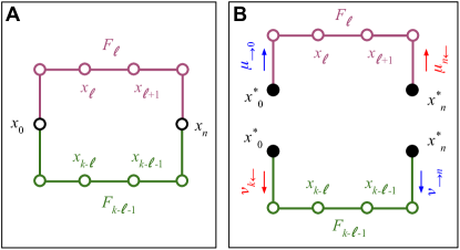
Figure 3: Belief propagation on cycles. (A) Factor graph with circular topology, in which belief propagation does not generally lead to the correct marginals Weiss-2000 . (B) By conditioning on $x_{0}$ and $x_{n}$ (black filled circles) we effectively turn the cycle into two chains—one “external” (purple) and another “internal” (green)—with $x_{0}$ and $x_{n}$ clamped to some given values $x_{0}^{\ast}$ and $x_{n}^{\ast}$. Such clamping can be implemented via initial and final marginals $p_{0}(x_{0})=\delta(x_{0}-x_{0}^{\ast})$ and $p_{n}(x_{n})=\delta(x_{n}-x_{n}^{\ast})$. More generally, we can fix generic marginals $p_{0}$ and $p_{n}$ and search for solutions consistent with them (see Appendix C.3).

Here we show that, using the cavity method of statistical mechanics, the dynamics of an embodied scientist performing an experiment can also be described in terms of the imaginary-time versions of the Schrödinger equation and the wave function, as well as their imaginary-time conjugates. The Born rule also arises naturally in this framework. We will focus only on the main points. In Appendix C.2 we provide a brief introduction to the cavity method.

The cavity method is exact on graphical models without loops. So, let us first neglect the term $\widetilde{F}_{n}$ in Eq. (3) to obtain a graphical model on a chain, consisting of factors $F_{0},\dotsc,F_{n-1}$, rather than on a cycle. We will return to the case of a cycle afterwards.

If we remove variable $x_{\ell}$, i.e., if we make a cavity to the graphical model, the original chain going from $x_{0}$ to $x_{n}$ would split into two chains: the “past” and “future” of $x_{\ell}$, so to speak, which contain variables $x_{0}$ and $x_{n}$, respectively. The cavity messages $\mu_{\to\ell}$ and $\mu_{\ell\leftarrow}$, respectively, summarize the influence on $x_{\ell}$ from the “past” and “future” chains, respectively, so that the probability marginal at time step $\ell$ is given by

$$p_{\ell}(x)=\mu_{\to\ell}(x)\mu_{\ell\leftarrow}(x).$$ (22)

This is a standard result of the cavity method Mezard-book-2009 (ch. 14; see also Eq. (145) in Appendix C.2 herein).

The cavity messages can be computed recursively via the cavity equations, i.e. Mezard-book-2009 (ch. 14; see also Eqs. (149) and (150) in Appendix C.2 herein),

$$\mu_{\to\ell+1} = F_{\ell}\mu_{\to\ell},$$ (23)

$$\mu_{\ell\leftarrow} = \mu_{\ell+1\leftarrow}F_{\ell},$$ (24)

which are valid for $\ell=0,\dotsc,n-1$. Here the factors $F_{\ell}$ are interpreted as matrices, the forward cavity messages $\mu_{\to\ell}$ as column vectors, the backward cavity messages $\mu_{\ell\leftarrow}$ as row vectors, and the right hand side of Eqs. (23) and (24) as dot products. Equations (23) and (24) propagate information from “past” to “future” and from “future” to “past”, respectively. The iteration of the cavity messages according to the cavity equations is called belief propagation (BP).

In the case of a chain, the initial cavity messages of the BP recursion, Eqs. (23) and (24), can always be selected equal to a constant, i.e., $\mu_{\to 0}(x)\propto 1$ and $\mu_{n\leftarrow}(x)\propto 1$, since there are no factors either before $x_{0}$ or after $x_{n}$. In principle, arbitrary initial probability distributions $p_{0}(x_{0})$ could be prepared via a suitable potential energy $V_{\rm prep}(x_{0})$ influencing only variable $x_{0}$.

Although the BP recursion is not exact on cycles, if we know the initial and final probability marginals, $p_{0}$ and $p_{n}$, we can effectively turn the cycle into two chains (see Fig. 3 and Appendix C.3)—we continue focusing only on the external chain. In this case we can then search for cavity messages that are consistent with both the BP recursion, Eqs. (23) and (24), as well as with the initial and final marginals, $p_{0}(x)=\mu_{\to 0}(x)\mu_{0\leftarrow}(x)$ and $p_{n}(x)=\mu_{\to n}(x)\mu_{n\leftarrow}(x)$. This yields a set of equations that turn out to be equivalent to those investigated in detail by Zambrini in the context of imaginary-time quantum dynamics zambrini1986stochastic (see Eqs. (2.6), (2.16), (2.22), and (2.23) therein; $\mu_{\to\ell}$, $\mu_{\ell\leftarrow}$, and $F_{\ell}$ here correspond, respectively, to $\theta^{\ast}$, $\theta$, and $h$ therein). Unlike with chains, the initial cavity messages of the BP recursion in a cycle, $\mu_{\to 0}$ and $\mu_{n\leftarrow}$, cannot generally be selected as constants anymore. This is because they now play a key role in effectively turning the cycle into two chains. So, cycles can entail a non-trivial BP dynamics with generic initial cavity messages. As we will now see, these dynamics are indeed described by the Schrödinger equation and its adjoint.

Introducing Eq. (12) into Eqs. (23) and (24) we get

$$\mu_{\to\ell+1}-\mu_{\ell} = \epsilon J_{\ell}\mu_{\to\ell}+O(\epsilon^{2}),$$ (25)

$$-(\mu_{\ell+1\leftarrow}-\mu_{\ell\leftarrow}) = \epsilon\mu_{\ell\leftarrow}J_{\ell}+O(\epsilon^{2}).$$ (26)

Taking the continuous-time limit, $\epsilon\to 0$ and $t=\ell\epsilon$, and writing $J_{\ell}=-H/{\Gamma}$ we get

$$-{\Gamma}\frac{\partial\mu_{\to}}{\partial t} = H\mu_{\to},$$ (27)

$${\Gamma}\frac{\partial\mu_{\leftarrow}}{\partial t} = \mu_{\leftarrow}H,$$ (28)

where $\mu_{\to}(t)=\mu_{\to\ell}$ and $\mu_{\leftarrow}(t)=\mu_{\ell\leftarrow}$ are considered as column and row vectors, respectively. Equations (27) and (28) are the imaginary-time Schrödinger equation and its adjoint, respectively, where ${\Gamma}$, $\mu_{\to}$ and $\mu_{\leftarrow}$ play the role of Planck’s constant, the imaginary-time wave function and its conjugate, respectively (cf. Eq. (21)). Indeed, Eqs. (27) and (28) are formally analogous to Eqs. (2.1) and (2.17) in Ref. Zambrini-1987 , where imaginary-time quantum dynamics is extensively discussed—the analogous of $\theta$ and $\theta^{\ast}$ therein are here $\mu_{\leftarrow}$ and $\mu_{\to}$, respectively. The analogue of the Born rule is naturally given by the continuous-time limit of the standard BP rule, Eq. (22).

II.4.4 Example: Two-slit experiment in imaginary time

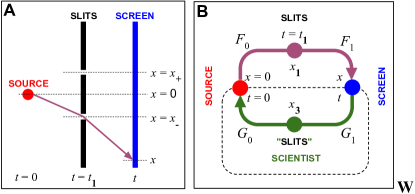
Figure 4: Two-slit experiment: (A) A classical particle initially at (vertical) position $x=0$ at time $t=0$ goes at time $t=t_{1}$ through a barrier with two slits, located at positions $x_{\pm}=\pm x_{\rm slit}$, and hits a screen at a generic position $x$ at a generic time $t$. Slits can be open or closed. (B) Factor graph associated to a scientist performing a two-slit experiment. The real non-negative factors $F_{0}$ and $F_{1}$ capture the “external” dynamics between the source and the slits, and between the slits and the screen, respectively. Factors $G_{0}$ and $G_{1}$ captures the dynamics “internal” to Wigner’s friend. Here $x_{3}$ refers to the “internal” physical correlate of the position of the slits. When only one slit is open, say the slit located at $x_{+}$, consistency requires that $x_{1}=x_{3}=x_{+}$. However, when both slits are open, $x_{1}$ does not have to equal $x_{3}$ anymore, which yields the imaginary-time version of quantum interference.

Here we consider the specific instance of a scientist doing a classical two-slit experiment (see Fig. 4). We will see that it coincides with the imaginary-time version of the standard quantum two-slit experiment. Consider a path $\widetilde{\mathbf{x}}=(x_{0},x_{1},x_{2},x_{3})$ that starts at the source located at $x_{0}=0$ at $t_{0}=0$ and goes through $x_{1}\in\{x_{+},x_{-}\}$, $x_{2}=x$, and $x_{3}$ at times $t_{1}$, $t_{2}=t$, and $t_{3}$, respectively, to return to $x_{4}=x_{0}=0$. Here $x_{3}$ is associated to the physical correlates of the slits “internal” to the scientist in Fig. 4, so $x_{3}\in\{x_{+},x_{-}\}$ too. With this notation, following Eq. (3), the probability associated to the path $\widetilde{\mathbf{x}}$ is

$$\widetilde{\mathcal{P}}(\widetilde{\mathbf{x}})=G_{0}(x_{4},x_{3})G_{1}(x_{3},x_{2})F_{1}(x_{2},x_{1})F_{0}(x_{1},x_{0}).$$ (29)

If one of the two slits is closed, the particle can only go through one of them at time $t_{1}$. That is, $x_{1}=x_{\pm}$ where the upper and lower sign denotes the situation where the particle goes through the upper and lower slit, respectively. In this case, the probability to find the particle at position $x_{2}=x$ at time $t_{2}=t$ is given by

$$\mathcal{P}_{\pm}(x,t)\equiv\tfrac{1}{Z_{\rm one}}\widetilde{\mathcal{P}}(0,x_{\pm},x,x_{\pm}),$$ (30)

where

$$Z_{\rm one}={Z_{\pm}}\equiv\int\mathcal{P}(0,x_{\pm},x,x_{\pm})\mathrm{d}x,$$ (31)

ensures that $\mathcal{P}_{\pm}$ is normalized. Due to the symmetry between slits, we have that $Z_{\pm}=Z_{\rm one}$ is the same for both $x_{\pm}$.

Following Eqs. (29) and (30) we can write

$$\tfrac{1}{\sqrt{Z_{\rm one}}}F_{0}(x_{\pm},0)F_{1}(x,x_{\pm}) = \sqrt{\mathcal{P}_{\pm}(x,t)}e^{S_{\pm}(x,t)},$$ (32)

$$\tfrac{1}{\sqrt{Z_{\rm one}}}G_{1}(x_{\pm},x)G_{0}(0,x_{\pm}) = \sqrt{\mathcal{P}_{\pm}(x,t)}e^{-S_{\pm}(x,t)},$$ (33)

which defines the imaginary-time phases $S_{\pm}$.

If the two slits are open, instead, then the probability for the particle to be located at position $x_{2}=x$ at time $t_{2}=t$ is given by

$$\begin{split}\mathcal{P}_{\rm both}(x,t)&\equiv\tfrac{1}{Z_{\rm both}}\sum_{x_{1},x_{3}\in\{x_{+},x_{-}\}}\mathcal{P}(0,x_{1},x,x_{3})\\ &=C\left\{\frac{1}{2}\left[\mathcal{P}_{+}(x,t)+\mathcal{P}_{-}(x,t)\right]+\mathcal{I}\right\}\\ \end{split}$$ (34)

where $Z_{\rm both}$ is a normalization constant, $C={2Z_{\rm one}}/{Z_{\rm both}}$, and

$$\mathcal{I}=\sqrt{\mathcal{P}_{+}(x,t)\mathcal{P}_{-}(x,t)}\cosh\left[\Delta S(x,t)\right]$$ (35)

with

$$\Delta S(x,t)=S_{+}(x,t)-S_{-}(x,t).$$ (36)

The first two terms in the second line of Eq. (34) come from the elements of the sum with $x_{1}=x_{3}=x_{\pm}$ (see Eq. (30)). The last term in the second line of Eq. (34), which is the imaginary-time interference term, comes from the elements of the sum with $x_{1}\neq x_{3}$, i.e.,

$$\widetilde{\mathcal{P}}(0,x_{+},x,x_{-}) = Z_{\rm one}\sqrt{\mathcal{P}_{+}(x,t)\mathcal{P}_{-}(x,t)}e^{\Delta S},$$ (37)

$$\widetilde{\mathcal{P}}(0,x_{-},x,x_{+}) = Z_{\rm one}\sqrt{\mathcal{P}_{+}(x,t)\mathcal{P}_{-}(x,t)}e^{-\Delta S}.$$ (38)

The right hand side of these equations is obtained by using Eqs. (32) and (33).

According to Eq. (34), the sum rule of classical probability theory, i.e.,

$$\mathcal{P}_{\rm both}(x,t)\neq\frac{1}{2}\left[\mathcal{P}_{+}(x,t)+\mathcal{P}_{-}(x,t)\right].$$ (39)

is not satisfied in this context. This is analogous to the phenomenon of quantum interference. Indeed, if we change the hyperbolic cosine in Eq. (35) for a cosine, i.e., doing $\cosh\to\cos$, Eq. (34) coincides exactly with the formula for the actual quantum two-slit experiment. In other words, Eq. (34) describes the imaginary-time version of quantum interference. Indeed, since the factors in Eqs. (32) and (33) are products of factors like those in Eqs. (5) in the main text, the phases $S_{\pm}(x,t)$ are proportional to the time step $\epsilon$. So, under a Wick rotation $\epsilon\to i\epsilon$ the right hand side of Eqs. (32) and (33) turn into complex wave functions and the hyperbolic cosine turns into a cosine, since $\cos(iz)=\cosh(z)$ for any $z$.

II.4.5 A few comments

To recap, we have shown that scientists can obtain a seemingly observer-independent view of the world at the price of describing it in terms of a real probability matrix that follows an imaginary-time quantum dynamics. This suggests the first property that observer’s should have, i.e.:

O1. Embodiment: The state of an observer explicitly described as a physical object, i.e., an “observer-as-object,” (see Sec. III.3.1 below) interacting with an experimental system is given by a real probability matrix $P_{\ell}$. The diagonal elements of $P_{\ell}$ are the probabilities for the different outcomes of the experiment to occur. $P_{\ell}$ follows a dynamics given by (see Eq. (16))

$$\Delta P_{\ell}=\epsilon[J_{s},P_{\ell}],$$ (40)

where $\Delta P_{\ell}=P_{\ell+1}-P_{\ell}$, $\ell$ denotes the time step and $\epsilon$ is the time step size.

Equivalently, scientists can also describe the world in terms of forward and backward BP cavity messages, which are formally analogous to imaginary-time wave functions and their conjugates. These forward and backward BP cavity messages, respectively, follow a BP dynamics described by the imaginary-time Schrödiner equation and its conjugate. However, we here focus on probability matrices because these directly yield probabilistic information, unlike BP messages that must be multiplied by another object—its “conjugate”—to do so.

Of course, scientists can also use standard probability distributions, if they prefer so. However, they cannot do it in terms of a single-variable marginal, on variables $x_{\ell}$, evolving according to a Markovian rule. Scientists would have to use a Bernstein process instead and would have to specify a two-variable marginal as initial state (see Eq. (9))—e.g., the probability for the initial and final states to have a certain value.

We have also shown how factor graph models with circular topology can be naturally described in terms of Markov-like chains formally analogous to imaginary-time quantum dynamics. These Markov-like chains are similar to the standard Markov chains, which naturally describe factor graph models with linear topology, except that the state of the system is described in terms of probability matrices rather than standard probability vectors. In this sense, Markov chains and imaginary-time quantum dynamics could be considered as instances of linear and circular causality, respectively.

Interestingly, imaginary-time quantum dynamics already displays some quantum-like features Zambrini-1987 . For instance, using our framework we have shown that a classical two-slit experiment can entail constructive interference. This provides a fresh perspective to think about quantum interference. When an embodied observer has information about which slit the particle goes through—e.g., when only one slit is open—this has to be reflected in the physical correlates of the experiment “internal” to her. So, the variable $x_{1}$ describing the slit, which is external to the observer, and the variable $x_{3}$, which is the corresponding physical correlate internal to the observer, must be equal, i.e., $x_{3}=x_{1}$ (see Fig. 4). In this view, the imaginary-time version of quantum interference arises because, when an embodied observer cannot access any information about which slit the particle goes through, the values of $x_{1}$ and $x_{3}$ do not have to coincide even though they refer to the same “thing” (i.e., the slits). This would be true no matter the reason for which the embodied observer lacks “which-way” information. Furthermore, our approach considers the whole experimental setup, or context, from beginning to end. So, it could also potentially take account of variations of the two-slit experiments, such as delay choice or quantum erasure experiments.

Following the tradition in physics, we have focused on the dynamics external to the scientist. However, similar results can be obtained if, following the tradition in cognitive science, we focus on the dynamics internal to the scientist, instead, and consider the external system as hidden to her—this could be done by marginalizing $\widetilde{\mathcal{P}}$ in Eq. (2) over the external paths instead of marinalizing it over the internal paths as we have done. That is, we could obtain an equation from $\ell=n\dotsc,k-1$, similar to Eq. (11), if we focus on the physical correlates of the experimental system, which are internal to the observer, rather than on the experimental system itself, which is external to the observer.

Up to now we have focused on the case of a well-known so-called “stoquastic” Hamiltonian $H$ (see Eq. (13). However, we will describe more general Hamiltonians later on.

It seems natural to wonder what about actual, real-time quantum dynamics. Up to now we have considered a scientist $F$ performing an experiment with a generic physical system $S$. However, $F$ is also a physical system. So, the combined system $S_{\rm coup}=F+S$ that we have modeled is also a physical system. In our previous analysis $S_{\rm coup}$ appears as an observer-independent physical system. Consistency would require that such an observer also be included in the action-perception loop. It turns out that properly dealing with this situation can lead to complex density matrices and real-time quantum dynamics. We will discuss this in Sec. III.

II.4.6 Internal and external dynamics are related by an “apparent time reversal”

Here we show that, if the dynamics external to the observer is described by the probability matrices $P_{\ell}$ and factors $F_{\ell}$, the internal dynamics is described by their transposed, i.e., $P_{\ell}^{T}$ and $F_{\ell}^{T}$. Indeed, in the example of the two-slit experiment we have an external variable, $x_{1}$, characterizing the slits and a corresponding internal variable, $x_{3}$, characterizing the scientist’s physical correlates associated to her perception of the slits (see Fig. 4). These two variables have the same domain, $x_{1},x_{3}\in\{x_{-},x_{+}\}$, because they refer to the same phenomenon, i.e., the slits. In a sense, variable $x_{3}$ is essentially the physical correlate of variable $x_{1}$.

If the scientist knows which slit the particle goes through, e.g., if one of the slits is closed, then these two variables have to coincide with the observed value, $x_{1}=x_{3}=x_{\rm obs}$. This constrain effectively reduces those two variables to one. Similarly, there is only one instance of the initial and final variables, $x_{0}$ and $x_{n}$ (here $n=2$), respectively, because the scientist in principle knows the initial state she prepares and the final state she measures. However, if the scientist does not know which slit the particle goes through, i.e., if variable $x_{1}$ is unobserved, $x_{1}$ and $x_{3}$ do not have to coincide and this can lead to the imaginary-time version of quantum interference.

We will write $y_{1}=x_{3}$ to emphasize that $x_{3}$ is the physical correlate of $x_{1}$. Similarly, $y_{0}=x_{2n}=x_{0}$ and $y_{n}=x_{n}$ (here $n=2$)—these are variables observed by $F$, so they are actually the same for the external and internal paths. With this notation the external and internal paths can be written as $x_{0}\to x_{1}\to x_{n}$ and $y_{n}\to y_{1}\to y_{0}$, respectively, which emphasizes that the internal and external dynamics flow in the opposite directions (see Fig. 2C). When the observer observes the slits we have that $y_{1}=x_{1}$ too; in this case the internal path is literally the time reversal of the external path.

The external and internal dynamics, respectively, are characterized by the chain of factors $F_{1}(x_{2},x_{1})F_{0}(x_{1},x_{0})$ and $G_{0}(y_{0},y_{1})G_{1}(y_{1},y_{2})$ (see Eq. (29)). Factors $G_{0}$ and $G_{1}$, respectively, can also be interpreted as the physical correlates of factors $F_{0}$ and $F_{1}$. The observer knows with certainty the functional form of factors $F_{\ell}$ since the Hamiltonian function, $\mathcal{H}$, which characterizes the experimental system, as well as the time parameter are known by her—the only physically relevant information that the observer can ignore in this example are the values of the variables associated to the slits. Hence, the two factors must essentially coincide.

Indeed, if the internal dynamics accurately reflect the external dynamics then the factors $G_{\ell}$, which characterizes the internal dynamics should equal the corresponding factors $F_{\ell}$ that characterizes the external dynamics, except for the fact that the two dynamics flow in opposite directions. That is, $G_{0}(y_{0},y_{1})=F_{0}(y_{1},y_{0})$ and $G_{1}(y_{1},y_{2})=F_{1}(y_{2},y_{1})$ or, in matrix notation, $G_{0}=F_{0}^{T}$ and $G_{1}=F_{1}^{T}$. The transpose appears because the internal and external paths are traversed in opposite directions. So, marginalizing over all variables, except $x_{0}$ and $y_{0}$, we get $P_{0}=F^{T}_{0}F_{1}^{T}F_{1}F_{0}$, which is symmetric. As we already know, the dynamics is obtained via the permutation of factors from right to left. Permuting factors yields $P_{1}=F_{0}F^{T}_{0}F_{1}^{T}F_{1}$, $P_{2}=F_{1}F_{0}F^{T}_{0}F_{1}^{T}$, which is also symmetric, and $P_{3}=F_{1}^{T}F_{1}F_{0}F^{T}_{0}=P_{1}^{T}$. Thus, if the external dynamics is described by the terms $P_{\ell}$ and $F_{\ell}$, the internal dynamics is described by their transposed, i.e., $P_{\ell}^{T}$ and $F_{\ell}^{T}$.

More generally, for every external unobserved variable, $x_{\ell}$ for $\ell=1,\dots n-1$, characterizing a given external phenomenon, there should be a corresponding internal variable characterizing the scientist’s physical correlates associated to her perception of such a phenomenon. So, the external and internal paths, $x_{0}\to x_{1}\to\cdots\to x_{n-1}\to x_{n}$ and $x_{n}\to x_{n+1}\to\cdots\to x_{k-1}\to x_{k}$, should be divided into the same number of time steps, i.e., $k=2n$. Furthermore, the internal path effectively runs from $x_{n}$ to $x_{k}=x_{0}$, which is the reverse direction of the external path, which runs from $x_{0}$ to $x_{n}$. So, for instance, the internal variable corresponding to the unobserved external variable $x_{n-1}$ is $y_{n-1}=x_{n+1}$. In general, the internal variable $y_{\ell}=x_{2n-\ell}$ corresponds to the unobserved external variable $x_{\ell}$.

The influence between the external variables $x_{\ell}$ and $x_{\ell+1}$ is characterized by the factor $F_{\ell}(x_{\ell+1},x_{\ell})$, for $\ell=0,\dotsc,n-1$. The influence between the corresponding internal variables $y_{\ell}=x_{2n-\ell}$ and $y_{\ell+1}=x_{2n-\ell-1}$ is characterized by the factor $G_{\ell}(y_{\ell+1},y_{\ell})$ for $\ell=0,\dotsc,n-1$. If the scientist have reached an accurate description of the experimental system, her physical correlates should perfectly reflect it. In other words, the internal and external dynamics should essentially mirror each other. That is,

$$G_{\ell}=F_{\ell}^{T}$$ (41)

for $\ell=0,\dotsc,n-1$. Using Eq. (41), Eq. (10) can be written as

$$\begin{split}P_{\ell}&=\frac{1}{Z}F_{\ell-1}\cdots F_{0}G_{0}\cdots G_{n-1}F_{n-1}\cdots F_{\ell}\\ &=\frac{1}{Z}F_{\ell-1}\cdots F_{0}F_{0}^{T}\cdots F_{n-1}^{T}F_{n-1}\cdots F_{\ell},\end{split}$$ (42)

for $\ell=0,\dotsc,n-1$. Further permuting factors we can obtain the dynamics from time $n$ on, which yields for time step $2n-\ell\geq 0$ (with $\ell=0,\dotsc,n-1$)

$$\begin{split}P_{2n-\ell}&=\frac{1}{Z}G_{\ell}\cdots G_{n-1}F_{n-1}\cdots F_{0}G_{0}\cdots G_{\ell+1}\\ &=\frac{1}{Z}F_{\ell}^{T}\cdots F_{n-1}^{T}F_{n-1}\cdots F_{0}F_{0}^{T}\cdots F_{\ell-1}^{T}=P_{\ell}^{T}.\end{split}$$ (43)

$P_{2n-\ell}$ describes the internal dynamics in the same order of the external dynamics, i.e., from $x_{k}=x_{0}$ to $x_{n}$. Equation (43) indicates that such dynamics is the transposed of the external dynamics. Therefore, since the external dynamics is given by Eq. (16), then the internal dynamics from $x_{0}$ to $x_{n}$ is given by its transpose, i.e., $\partial P^{T}/\partial t=-[J^{T},P^{T}]$. Notice that the initial and final probability matrices in this case are symmetric, i.e., $P_{0}=P_{0}^{T}$ and $P_{n}=P_{n}^{T}$.

III Reflexivity and real-time quantum dynamics

According to the analysis in Sec. II, summarized in observer property O1 (see Sec. II.4.5), scientists can in principle “escape” the action-perception loop and describe classical systems in an effective, seemingly observer-independent way by describing such systems in terms of real-valued probability matrices that follow an imaginary-time quantum dynamics. This suggests that the observer might indeed be key to the quantum formalism, as emphasized in QBism debrota2018faqbism ; mermin2018making ; fuchs2014introduction . However, the actual quantum formalism does not take place in imaginary time, but in real time.

Here we explore how real-time quantum dynamics might relate to our model of embodied scientists doing experiments. To do so, we first rewrite von Neumann equation, Eq. (20), which is complex valued, as a pair of real equations related to its imaginary and real parts. We then show that these equations are related to the equations associated to an embodied scientist doing an experiment, Eq. (19) and its transposed via a “swap”operation. We also show how such a swap operation can naturally arise when two mirrors mutually reflect each other.

This suggests that we can obtain real-time quantum dynamics by reflexively coupling two (sets of) observers mutually observing each other. In this sense, observers are relative to each other rather than to an external, unacknowledged observer. We discuss an analogy with mirrors and video-systems to highlight some properties that will help us build the reflexive coupling between observers. We identify other eight observer’s properties that, along with observer’s property O1, enable us to extend our work to the case of real-time quantum dynamics—in particular, we have to distinguish two complementary roles of observers: that of subjects who observe or experience and that of objects being experienced by other subjects. In short, two (sets of) embodied observers involved in a reflexive coupling can entail a dynamics formally analogous to genuine real-time quantum dynamics.

III.1 Von Neumann equation as a pair of real equations

Actual quantum systems are generally described by a complex-valued density matrix $\rho$ satisfying the von Neumann equation, Eq. (20). In order to explore how the actual quantum dynamics relates to the imaginary-time quantum dynamics that we have obtained, which is real-valued, here we will separate its real and imaginary parts. To do so, we use the fact that the density matrix and the Hamiltonian are Hermitian operators, i.e., they are equal to their adjoints: $\rho^{\dagger}=\rho$ and $H^{\dagger}=H$. We will focus here on the common case where the adjoint operation $\dagger$ is given by the combination of transpose $T$ and complex conjugate $\ast$ operations, e.g., $[\rho^{\dagger}](x,x^{\prime})=[\rho(x^{\prime},x)]^{\ast}$. In this case we can write

$$\rho=P_{s}+P_{a}/i,$$ (44)

where $P_{s}=P_{s}^{T}$ and $P_{a}=-P_{a}^{T}$ are, respectively, some generic real-valued symmetric and antisymmetric matrices. Without loss of generality, we can write $P_{s}=(P+P^{T})/2$ and $P_{a}=(P-P^{T})/2$ as the symmetric and antisymmetric parts of a generic real matrix $P$. Since the diagonal elements of $P$ and $P^{T}$ are the same, these are equal to the diagonal elements of $\rho$. That is, the diagonal elements of $P$ are the actual probabilities encoded in $\rho$. So, when the off-diagonal elements of $P$ are non-negative, $P$ is a probability matrix like those we use in Sec. II.

We can write an equation for the Hamiltonian similar to Eq. (44), i.e.,

$$H=-\hbar J_{s}-\hbar J_{a}/i,$$ (45)

where $J_{s}=(J+J^{T})/2$ and $J_{a}=(J-J^{T})/2$ are the symmetric and antisymmetric parts of a generic real matrix $J$. We write $H$ in terms of $J$ so we do not have to worry about $\hbar$ below. When $J$ can be interpreted in probabilistic terms as above, e.g., when $H$ is given by Eq. (13), it is a dynamical matrix, with non-negative off-diagonal entries, much like those we used in Sec. (II). This suggests that $P$ and $J$ might actually be the most suitable objects to explore the potential relationship between genuine, real-time quantum dynamics and our framework.

Introducing $\rho=P_{s}+P_{a}/i$ and $H=-\hbar J_{s}-\hbar J_{a}/i$ in von Neumann equation, Eq. (20), and separating the real and imaginary parts, we get a pair of real-valued equations for $P_{s}$ and $P_{a}$, i.e.

$$\frac{\partial P_{s}}{\partial t} = [J_{s},P_{a}]+[J_{a},P_{s}],$$ (46)

$$\frac{\partial P_{a}}{\partial t} = -[J_{s},P_{s}]+[J_{a},P_{a}].$$ (47)

Adding and subtracting Eqs. (46) and (47) we get an equivalent pair of equations for $P$ and $P^{T}$, i.e.,

$$\frac{\partial P}{\partial t} = -[J_{s},P^{T}]+[J_{a},P],$$ (48)

$$\frac{\partial P^{T}}{\partial t} = [J_{s},P]+[J_{a},P^{T}].$$ (49)

Notice that Eq. (49) is the transposed of Eq. (48).

If the terms $-[J_{s},P^{T}]$ in Eq. (48) and $[J_{s},P]$ in Eq. (49) were swapped, Eqs. (48) and (49) would become

$$\frac{\partial P_{\rm swap}}{\partial t} = [J,P_{\rm swap}],$$ (50)

$$\frac{\partial P^{T}_{\rm swap}}{\partial t} = -[J^{T},P^{T}_{\rm swap}],$$ (51)

since $J=J_{s}+J_{a}$, which are the imaginary-time von Neumann equation, Eq. (19), and its transpose. According to our previous results, the former can be associated to an embodied scientist doing an experiment and the latter to the time reversal process.

So, it seems that this swap operation might help us bridge our approach with real-time quantum mechanics. For simplicity, since this swap operation only involves the terms with $J_{s}$, we will first focus on these terms by doing $J_{a}=0$ for now. So, taking $J_{a}=0$, discretizing Eqs. (50) and (51) for convenience and dropping the subindex “swap”, we have

$$\Delta P_{\ell} = \epsilon[J_{s,\ell},P_{\ell}],$$ (52)

$$\Delta Q_{\ell} = -\epsilon[J_{s,\ell},Q_{\ell}],$$ (53)

where $Q_{\ell}=P_{\ell}^{T}$. Intuitively, Eqs. (52) and (53) are related by a time-reversal, $\epsilon\to-\epsilon$—i.e., if Eq. (52) describes the circular process in Fig. 2C in a clockwise direction, then Eq. (53) will describe it in a counter-clockwise direction. We will formalize this later on.

III.2 Reflexive coupling: An analogy with mirrors and video feedback

III.2.1 An analogy with mirrors

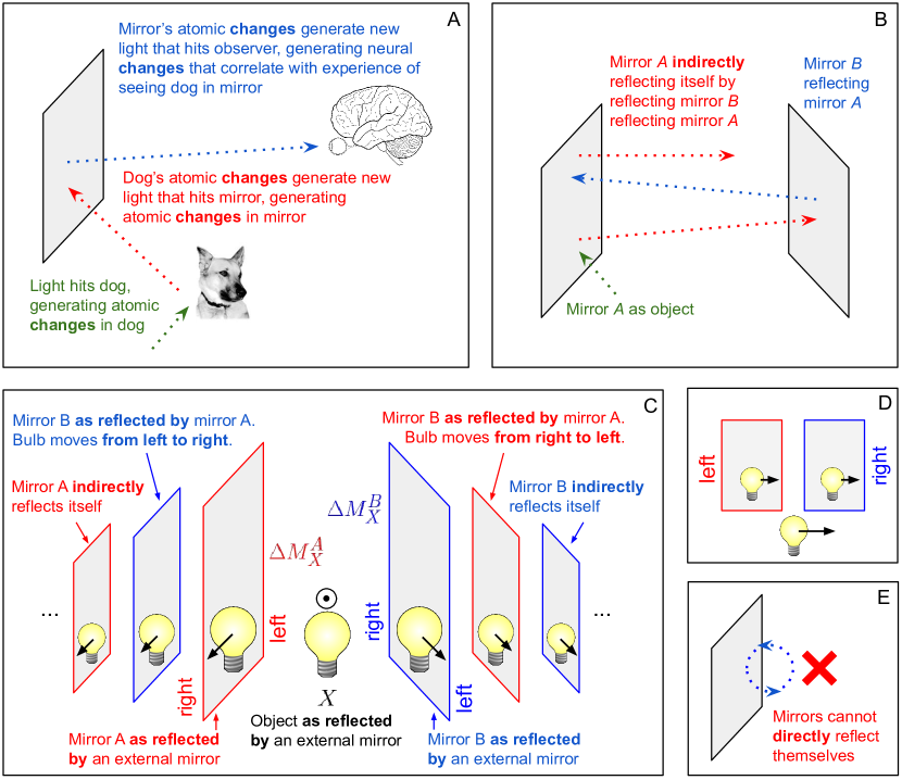
Figure 5: Some properties of mirrors: (A) How do mirrors reflect objects? When light hits an arbitrary object, say a dog, physical changes in the dog induce physical changes in the mirror which, through the observer’s eyes, induces changes in the observer’s neural patterns. These neural changes correlate with the experience of seeing the dog reflected in the mirror (see text). (B) Mirrors can indirectly reflect themselves. (C) If there is an object in between the two mutually reflecting mirrors (here a light bulb), they can reflect that object as well as each other reflecting that object. Mirrors $A$ and $B$ as well as the light bulb could also be a reflection in other mirror—say, the black rectangle in which the figure is framed. Importantly, if the object is moving, say, towards outside the page (denoted here by $\bigodot$) then it would appear to the (red) mirror $A$ as moving from left to right and to the (blue) mirror $B$ as moving from right to left instead. We refer to this as an “apparent time reversal.” (D) If there is no reflexive coupling between mirrors, i.e., if the mirrors are not facing each other, but are rather parallel to each other, there is no “apparent time reversal” as they reflect the object moving in the same direction. (E) Mirrors cannot directly reflect themselves.

We have seen that a swap operation turns genuine real-time quantum dynamics, given by Eqs. (48) and (49), into two independent imaginary-time quantum dynamics, given by Eqs. (50) and Eq. (51) which are formally analogous to the equation describing an embodied observer, Eq. (19), and its transposed. An analogous swap operation appears when studying reflexive systems such as mirrors. It will then be useful to discuss some aspects of mirror reflection.

In this analogy with mirrors, “reflection” is analogous to “experience” or “observation”. That is, mirrors reflecting objects are analogous to observers experiencing or observing phenomena. In a sense, observers could also “reflect” phenomena by communicating them either through language at the conscious level, which is supported by physical processes such as air vibration patterns or ink patterns on paper, or through bioelectric signals at the unconscious level. Untrained observers and trained scientists, respectively, would be analogous to stained and stainless mirrors. We will focus on the latter.

Let us begin with some basic physics of mirror reflection. Consider the process of seeing an arbitrary object on a mirror—say, a dog (see Fig. 5A). When light hits a dog, it induces some physical changes in the dog. Those changes can be energy changes—e.g., some atoms of the dog’s body absorb photons and get excited. Such changes produce other physical changes—e.g., the dog’s excited atoms can emit photons and relax. These changes in turn generates new light that hits the mirror inducing some physical changes—e.g., the mirror’s silver atoms absorb photons, get excited, and then re-emit those photons. Those changes produce more light which can hit the observer’s eyes producing some physical changes in the eye’s atoms. Finally, these changes can induce changes in the patterns of neural activity, changes that correlate with the experience of seeing the dog reflected on the mirror.

In summary, physical changes in the dog induce physical changes in the mirror which, through the observer’s eyes, induces changes in the observer’s neural patterns. These neural changes correlate with the experience of seeing the dog reflected in the mirror. In line with this, the first aspect of mirror reflection that we want to consider is the following:

M1. Mirrors reflect objects via physical changes—internal and external. A mirror reflects an object via the physical changes that light induces on the object. These changes, which are external to the mirror, generate light that induces physical changes on the mirror. These new changes, which are internal to the mirror, in turn generate light that induces physical changes on the observer. These latter changes correlate with the experience of seeing the object reflected on the mirror (see Fig. 5A). In directly reflecting an object, the mirror engages two rays of light: one incoming and one outgoing (red and blue arrows in Fig. 5A, respectively).

Accordingly, we will denote an arbitrary mirror $A$ reflecting a generic object $X$ as

$$\Delta M^{A}=\left.\Delta O^{X}\right|_{A}\equiv\boxed{\Delta O^{X}}_{A},$$ (54)

to emphasize that mirror reflection takes place via changes. Here the rectangle with subindex $A$ denotes mirror $A$. To avoid cluttering the paragraphs with rectangles, we have also introduced the alternative notation of a vertical bar with subindex $A$ (i.e., $\left.\right|_{A}$) to denote reflection in mirror $A$. We will use the same vertical bar to denote the analogue of reflection in other analogies, i.e., experience or observation in the case of observers, and recording-and-displaying in the case of video-systems.

So, mirrors can take objects as “input,” so to speak, and output their reflection. Importantly, an arbitrary mirror $A$ can also be the object being reflected by another arbitrary mirror $B\neq A$—this is denoted as $\Delta M^{B}=\left.\Delta M^{A}\right|_{B}$. In this sense, mirrors are analogous to computer programs or Turing machines. Indeed, computer programs not only take data as input, process them, but they (or, more precisely, their code) can also be the data that other computer programs take as the input to process. The former is an active role in that mirrors and computer programs perform a function—i.e., to reflect objects and to process data, respectively. The latter is a passive role in that mirrors and computer programs are just objects and data, respectively, that do not perform any function at all—rather, a function is performed on them. We can summarize this property of mirrors as follows:

M2. Mirrors play both active and passive roles. A mirror can both reflect other objects and be the object reflected by other mirrors. The latter is a passive role: mirror as object. The former is an active role: mirror as object-reflecting “subject,” so to speak—here “subject” is used in a strict technical sense as the opposite of object.

It is well known that two mirrors can recursively reflect each other, producing a so-called “infinite mirror” effect (see Fig. 5B). If there is an object in between the two mirrors, each mirror will reflect both the object and the other mirror reflecting the object (see Fig. 5C). In this way, mirrors can indirectly reflect themselves, even though they cannot directly do so (see Fig. 5E). Importantly, the infinite mirror effect appears due to the size distortion, each image appearing smaller than the previous one in the recursion. We do not expect a similar distortion to occur in the case of observers. This shall become more clear when we discuss an analogy with video-systems (see Sec. III.2.2).

This bring us to the next two properties of mirrors that we want to highlight:

M3. Mirrors can indirectly reflect themselves by reflexively coupling to other mirrors. According to M1, physical changes in mirror $A$ can induce changes in mirror $B\neq A$, which can in turn induce further changes in mirror $A$. At this point, mirror $A$ is reflecting an image of itself. However, in contrast to the direct reflection described in M1, here mirror $A$ engages four rays of light instead of two: two incoming and two outgoing (see Fig. 5B). In this sense, mirror $A$ indirectly reflects an image of itself. Moreover, this process of mutually reflecting the physical changes of each other continues ad infinitum, producing the well-known “infinite mirror” effect—this effect is due to size distortion and is not expected to occur in the case of observers. Importantly, each of these changes is external to one mirror and internal to the other; none of these changes can be both internal and external to the very same mirror (see Fig. 5B). If there is an object in between the two mirrors, each mirror will reflect both the object and the other mirror reflecting that same object (see Fig. 5C).

M4. Mirrors cannot directly reflect themselves. This would imply that the associated physical changes can simultaneously be both internal and external to the very same mirror, contradicting the situation described in M3 (see Fig. 5E). Similarly, a mirror cannot directly reflect its own internal changes because these are the very changes that allow the mirror to reflect any external changes at all—i.e., changes induced by light on objects external to the mirror. There is nothing mystical about this. This does not imply that the mirror is not a physical object; of course, it is. It only implies that the mirror’s internal changes are fundamentally inaccessible to the mirror itself, they will always remain implicit—of course, these changes can be accessed and reflected by another mirror (see Fig. 5 B).

Property M4 suggests that every perspective has a blindspot. The situation is analogous to that of an eye that can directly “see” any objects in its visual field, but it cannot directly see itself—of course, it can “see” an image of itself, say, in a mirror.

To formalize the situation illustrated in Fig. 5C, consider two mirrors $A$ and $B$ which are reflected by other mirrors, say $W$ and $W^{\prime}$, respectively. That is,

$$\Delta M^{W} = \left.\Delta M^{B}\right|_{W}\equiv\boxed{\Delta M^{B}}_{W},$$ (55)

$$\Delta M^{W^{\prime}} = \left.\Delta M^{A}\right|_{W^{\prime}}\equiv\boxed{\Delta M^{A}}_{W^{\prime}}.$$ (56)

In the particular case in which $W=A$ and $W^{\prime}=B$, Eqs. (55) and (56) describe the situation illustrated in Fig. 5C when mirrors $A$ and $B$ mutually reflect each other, i.e.,

$$\Delta M^{A} = \left.\Delta M^{B}\right|_{A}\equiv\boxed{\Delta M^{B}}_{A},$$ (57)

$$\Delta M^{B} = \left.\Delta M^{A}\right|_{B}\equiv\boxed{\Delta M^{A}}_{B}.$$ (58)

Equation (58) indicates that mirror $B$ is reflecting mirror $A$. Introducing this into Eq. (57) yields $\Delta M^{A}=\left.\left.\Delta M^{A}\right|_{B}\right|_{A}$. Similarly, Eq. (57) indicates that mirror $A$ is reflecting mirror $B$. Introducing this into Eq. (58) yields $\Delta M^{B}=\left.\left.\Delta M^{B}\right|_{A}\right|_{B}$. Continuing this process recursively yields the infinite-mirror effect, i.e.,

$$\Delta M^{A} = \boxed{\boxed{\boxed{\dots}_{A}}_{B}}_{A},$$ (59)

$$\Delta M^{B} = \boxed{\boxed{\boxed{\dots}_{B}}_{A}}_{B}.$$ (60)

Importantly, Eqs. (59) and (60) seems to describe a situation of two empty mirrors reflecting each other, but no other generic objects like the light bulb in Fig. 5C. However, this not so. It appears to be so because we have left the other generic object implicit to avoid cluttering the notation. We could make such a generic object $X$ explicit so that it becomes clear that mirrors $A$ and $B$ both reflect $X$ and reflect each other reflecting $X$. To do so, it is useful to make explicit that each of the two mirrors is reflecting two objects: (i) a generic object $X$—e.g., a light bulb; and (ii) the other mirror. This is analogous to a computer program having two input channels. To distinguish between these two kinds of objects we could simply write $\Delta M^{A}_{X}$ to denote a mirror $A$ reflecting a generic object $X$, and write $\Delta M^{A}_{X}=\left.\Delta M^{B}_{Y}\right|_{A}^{X}$ to denote a mirror $A$ which is reflecting both a generic object $X$ and another mirror $B$ that is directly reflecting a generic object $Y$. However, here we are interested only in the situation where there is only one and the same generic object $X$ being reflected by all mirrors, i.e., $Y=X$. So, we can just leave $X$ implicit.

Nevertheless, it will be useful to explicitly consider the case shown in Fig. 5C of two mirrors reflecting an object moving parallel to the mirrors towards outside the page (denoted in the figure by $\bigodot$). If mirror $A$ reflects the object as moving from its left to its right (see Fig. 5C), which is denoted as $\Delta M^{A}_{\to}$, then mirror $B$ reflects the object as moving in an opposite direction, i.e., from its right to its left, which is denoted as $\Delta M^{B}_{\leftarrow}$. In this case, the analogue of Eqs. (59) and (60) are

$$\Delta M^{A}_{\to} = \boxed{\overrightarrow{\boxed{\overrightarrow{{\boxed{\dotsc}_{A}}}}_{B}}}_{A},$$ (61)

$$\Delta M^{B}_{\leftarrow} = \boxed{\overleftarrow{\boxed{\overleftarrow{{\boxed{\dotsc}_{B}}}}_{A}}}_{B}.$$ (62)

Notice that if there is no reflexive coupling between mirrors, i.e., if the mirrors do not face each other, there is no arrow inversion (see Fig. 5D). This brings us to the next mirror property we want to highlight:

M5. Mirrors’ reflexive coupling involves an “apparent time-reversal”: Consider two reflexively coupled mirrors, $A$ and $B$, reflecting an external object. If the reflected object appears to move from left to right for mirror $A$, it would appear to move from right to left for mirror $B$. So, if from $A$’s perspective the object has velocity $v$, then from $B$’s perspective the object is moving with velocity $-v$. We will refer to this as an “apparent time-reversal.” Alternatively, if mirror $A$ registers a change in position $\Delta x^{A}=\epsilon v$ then mirror $B$ registers a change in position $\Delta x^{B}=-\epsilon v$—in this case we could also say that the “apparent time reversal” is manifested in the change $\epsilon\to-\epsilon$.

Of course, the object could move in a diagonal direction and only the horizontal component would be inverted. However, we have to keep in mind that this is only an analogy. We are taking into account only one dimension, the horizontal one, because in the reflexive coupling of observers there would be only one dimension too, the temporal labels.

The last mirror property we would like to highlight is that mirrors can only reflect relative changes. For instance, if in some frame of reference two reflexively coupled mirrors are moving with the same speed and in the same direction, they will reflect each other as being static (we are ignoring external objects for simplicity); it will not reflect the motion relative to that frame of reference—this is a simple instance of Galilean relativity. More precisely, we introduce the last mirror’s property:

M6. Mirrors can only reflect relative changes: Consider two reflexively coupled mirrors, $A$ and $B$, moving with velocities $v_{A|W}$ and $v_{B|W}$, respectively, relative to an external observer $W$—we ignore here external objects for simplicity. Mirrors $A$ and $B$ can “determine” their relative velocities, $v_{A|B}$ and $v_{B|A}$, but not the extrinsic velocity, $v_{C|W}$, of their centroid, $C$, relative to the external observer, $W$—the average or centroid velocity is $v_{C|W}=(v_{A|W}+v_{B|W})/2$. The corresponding velocities relative to the centroid are

$$v_{A|C} = v_{A|W}-v_{C|W},$$ (63)

$$v_{B|C} = v_{B|W}-v_{C|W}.$$ (64)

For $W$, the relative velocities between mirrors $A$ and $B$ are $v_{A|B}=2v_{A|C}$ and $v_{B|A}=2v_{B|C}$, respectively. So, mirrors $A$ and $B$ can “infer” the intrinsic velocities $v_{A|C}=-v_{B|C}$ by observing each other, but not the extrinsic velocity $v_{C|W}$ which only makes sense for $W$.

III.2.2 An analogy with video feedback

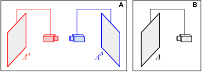
Figure 6: Video-feedback analogue of mirror-mirror reflection: (A) Two video-systems, $A$ and $B$, mutually recording-and-displaying each other. The video screens of systems $A$ and $B$ project images $\Lambda^{A}_{\ell}$ and $\Lambda^{B}_{\ell}$. (B) A single video-system can partially record-and-display itself. It cannot fully display itself, though; in particular, the camera cannot record itself.

To better understand the reflexive coupling between observers, we now resort to a more formal analogy with video-systems (see Fig. 6A). In this analogy, each mirror is analogous to a system composed of a video camera connected to a video screen. A mirror receiving light emitted by an object is analogous to the video camera of a video-system recording an object, and that same mirror reflecting the light received is analogous to the video screen displaying the object recorded by the video camera attached to it. In Fig. 6A the video camera of system $A$ records the video screen of system $B$ and vice versa. While the video camera of a single system can record the video screen of that same system (see Fig. 6B), the video camera cannot record itself. So, a video-system composed of both video camera and screen, which together are the analogue of a mirror, cannot completely record-and-display itself either.

Crutchfield crutchfield1984space analyzed the case shown in Fig. 6B, where only one video camera records the very same screen to which it is connected. He formalized the situation along the following lines: Let $\Lambda_{\ell}$ be the image displayed in the screen at time step $\ell$; that is, $\Lambda_{\ell}$ is a squared array of pixels, where each pixel can be any gray color, from white to black. The image at the next time step, $\ell+1$ is given by $\Lambda_{\ell+1}=\alpha\Lambda_{\ell}+\epsilon\mathcal{D}\left(\Lambda_{\ell}\right)$. The first term in the right hand side characterizes the memory of the system—when $\alpha=0$ the system does not remember the previous image. Here we are interested only in the case with $\alpha=1$. For this reason we will omit $\alpha$ from now on.

So, the video-system in Fig. 6B satisfies the equation

$$\Delta\Lambda_{\ell}=\epsilon\mathcal{D}\left(\Lambda_{\ell}\right).$$ (65)

Here $\Delta\Lambda_{\ell}\equiv\Lambda_{\ell+1}-\Lambda_{\ell}$, $\epsilon$ is the time step size and the function $\mathcal{D}$, characterizing the recording-and-displaying relation, can include, e.g., a rotation or a scaling of the image at time step $\ell$—i.e., by rotating or zooming in or out the video camera, respectively. The time step size, $\epsilon$, is introduced because we are interested in the limit $\epsilon\to 0$ when this difference equation becomes a differential equation.

As we already mentioned, the single video-system shown in Fig. 6B and described by Eq. (65) cannot record-and-display an image of itself since the video camera cannot record itself. A reflexive coupling between two video-systems, like two mirrors reflecting each other, can record-and-display an image of itself.

In analogy with mirrors, we can formalize the situation in Fig. 6A by first considering the situation in which a video-system $B$ record-and-display another video-system $A$, respectively. Let $\Lambda_{\ell}^{X}$ denote the state of video-system $X$ at time step $\ell$—here $X\in\{A,B\}$. At time step $\ell$ the states of the video-systems $A$ and $B$ are $\Lambda_{\ell}^{A}$ and $\Lambda_{\ell}^{B}$, respectively. Since the video-system $B$ is recording-and-displaying the video-system $A$, at time step $\ell+1$ the state of the video-system $B$ is $\Lambda^{B}_{\ell+1}=\Lambda^{B}_{\ell}+\epsilon\mathcal{D}_{B}\left(\Lambda_{\ell}^{A}\right)$ Importantly, the first term in the right hand side of this equation is $\Lambda_{\ell}^{B}$, not $\Lambda_{\ell}^{A}$, because this is a memory term—the video-system $B$ has memory about its own previous state, not about $A$’s. Similarly, the function $\mathcal{D}_{B}$ has the subindex $B$, not $A$, because it is the camera of video-system $B$ that captures and can transform (e.g., rotate or scale) an image of the video-system $A$. We can write this equation as

$$\Delta^{\rm i}\Lambda_{\ell}^{B}=\left.\Delta^{\rm e}\Lambda_{\ell}^{A}\right|_{B}^{\to}\equiv\epsilon\mathcal{D}_{B}\left(\Lambda_{\ell}^{A}\right),$$ (66)

where $\Delta^{\rm i}\Lambda_{\ell}^{B}=\Lambda_{\ell+1}^{B}-\Lambda_{\ell}^{B}$ are changes internal to the video-system $B$, as emphasized by the superindex “i.” In analogy with mirrors, we here denote by $\left.\Delta^{\rm e}\Lambda_{\ell}^{A}\right|_{B}^{\to}$ the changes in $A$ as recorded-and-displayed by the video-system $B$—these changes are external to the video-system $B$, as emphasized by the superindex “e.” In this case $\left.\Delta^{\rm e}\Lambda_{\ell}^{A}\right|_{B}$ is given by $\epsilon\mathcal{D}_{B}\left(\Lambda_{\ell}^{A}\right)$. Furthermore, the arrow $\to$ plays a role analogous to the arrow in Eq. (61), i.e., it indicates that Eq. (66) is one of a pair describing the reflexive coupling between video-systems $A$ and $B$. So, a reverse arrow $\leftarrow$ is analogous to the arrow in Eq. (62).

To complete the reflexive coupling we have to consider the case where $A$ and $B$ play the complementary roles of the “subject” that records-and-displays and the object being recorded-and-displayed. Agian, here the word “subject” is used in a strict sense to denote the opposite of object. In analogy with Eq. (66), this yields the equation

$$\Delta^{\rm i}\Lambda_{\ell}^{A}=\left.\Delta^{\rm e}\Lambda_{\ell}^{B}\right|_{A}^{\leftarrow}\equiv\epsilon\mathcal{D}_{A}\left(\Lambda_{\ell}^{B}\right).$$ (67)

Equations (66) and (67) are analogous to Eqs. (61) and (62) for mirrors. They implement the reflexive coupling between the video-systems $A$ and $B$.

We can now see more clearly that the infinite mirror effect appears due to a distortion in the size of the image. Indeed, consider the situation where both transformations $\left.\Delta^{\rm e}\Lambda^{B}_{\ell}\right|_{A}$ and $\left.\Delta^{\rm e}\Lambda^{A}_{\ell}\right|_{B}$ include only a scaling or zooming out of images by a factor $z\in[0,1]$, equal for both systems. An analogue of the infinite mirror effect would show up only when there is a non-zero scaling strictly less than one, i.e., $0<z<1$, because smaller images will recursively appear in the computer screen of systems $A$ and $B$. Indeed, iterating Eqs. (66) and (67) we obtain the analogues of Eqs. (61) and (62). However, when there is no scaling, $z=1$, this effect effectively disappears.

III.3 Reflexive coupling: Observers mutually observing each other

III.3.1 Scientists doing experiments are observed by other scientists

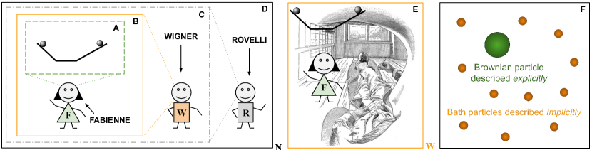
Figure 7: Escaping the infinite regress via the first-person perspective (figures A-D are nested): (A) Traditionally, physics focuses on the experimental system alone (inner green dashed box), effectively ignoring the observer. (B) Traditionally, cognitive science focuses on the observer (Fabbiene, Wigner’s friend) interacting with an experimental system (middle orange solid box), ignoring the external observer (Wigner) that observes the former. (C) Rovelli’s RQM Rovelli-1996 hints at the need to take explicit account of Wigner, as we do here. (D) However, this more relational perspective would still ignore the observer who is looking at Wigner. By adding another observer (Rovelli) we are headed to an infinite regress (cf. Fig. 5.1 in Ref. rovelli2007quantum ). One way to escape the infinite regress is by distinguishing between the first- and third-person perspectives, between observer-as-subject and observer-as-object (see text). (E) Please imagine that you take the role of Wigner in (C), so you are observing the situation depicted within the solid orange box from your own first-person perspective (1PP). The way you experience the situation is analogous to that of the gray man lying down in Mach self-portrait in (E). You can see Fabienne (and her experimental system), but you cannot see relevant aspects of yourself. Of course, you can see some aspects of yourself, e.g., parts of your body, but not the physical correlates associated to your experience of seeing Fabbiene, which are our focus here. We will represent the observer-as-subject with the rectangle within which the figure is framed; the letter in the bottom left of this rectangle indicates the observer-as-subject we are referring to. (F) The degrees of freedom of an observer-as-subject, represented by the man lying down in (E), are analogous to the degrees of freedom of a thermal bath in that they are inaccessible—however, the former are inaccessible in principle while the latter are inaccessible only in practice (see text). The degrees of freedom of an observer-as-object immersed in the field of experience of an observer-as-subject, so to speak, are analogous to those of a Brownian particle immersed in a thermal bath (see text).

Physical experiments are usually described as observer-independent systems (see Fig. 7A). This work aims at understanding how can scientists escape the action-perception loop to establish such a seemingly observer-independent science. To do so, we have been investigating the circular interaction between a scientist, Fabienne ($F$), and an external physical system, $S$ (see Fig. 7B; see also Figs. 1B and 2A). Now, not only $S$, but also Fabienne are physical systems. So, the coupled system, $S_{\rm coup}=F+S$, constituted by the scientist, $F$, interacting with the experimental system, $S$, can be considered as a physical system too.

This brings us back to the beginning of this work: we should not a priori describe any physical system—in particular $S_{\rm coup}$—as an observer-independent system. For our approach to be consistent we have to take into account the observer that observes $S_{\rm coup}$—let us call this observer Wigner ($W$; see Fig. 7C). That is, Wigner and $S_{\rm coup}$ are in principle also part of an action-perception loop. The role of Wigner is typically played by cognitive scientists who observe other human beings interact with the world—indeed, figures like Fig. 7B are common in the cognitive science literature. So, we need to ask: How can cognitive scientists too escape the action-perception loop and properly describe the coupled systems of humans and their surroundings as observer-independent systems? Indeed, much like experimental systems in physics, cognitive systems are often described in the literature as observer-independent.

Interestingly, this approach is in line with Rovelli’s relational interpretation of quantum mechanics (RQM), which posits that “the fact that a certain quantity $q$ has a value with respect to [an observer $F$] is a physical fact; as a physical fact, its being true, or not true, must be understood as relative to an observer, say $[W]$.” Rovelli-1996 (see Sec. II D therein). However, in RQM observers are considered as generic quantum system—i.e., as far as physics is concerned, there are no relevant differences between electrons and observers. In contrast, here we are treating observers as classical cognitive systems.

Figure 7C illustrates this. It shows a cognitive scientist (Wigner) looking at another scientist (Fabienne, Wigner’s friend) doing an experiment. In principle, we should build a model of Wigner interacting with his friend and the experimental system. But then again the coupled system $S^{\prime}_{\rm coup}=W+S_{\rm coup}$ of Wigner, his friend and the experimental system is also a physical system and would therefore be relative to another unacknowledged external observer. In principle, we could also make explicit such an additional external observer (Rovelli in Fig. 7D), but then we would be headed to an infinite regress. That is, we would have to keep on adding external observers ad infinitum.

This brings us to a potentially subtle point. One way to escape such an infinite regress involves two steps. First, we have to distinguish that observers, similar to mirrors, can play complementary roles as objects and as object-experiencing “subjects”—here the word “subject” is used in the strict technical sense of the opposite of object. Second, we have to implement a reflexive coupling between two (sets of) observers mutually observing each other.

Let us now describe the first of these two steps in more detail. Please look at Fig. 7E and imagine that you are experiencing the situation depicted in it—that is, imagine that you play the role of the man in Mach’s self-portrait. From a cognitive science perspective, when you look at the system $S_{\rm coup}=F+S$ depicted in Fig. 7E there is a physical interaction between you and $S_{\rm coup}$—e.g., light reflected from $S_{\rm coup}$ interacts with your eyes. Such a physical interaction generates physical processes inside you that correlate with your experience of observing $S_{\rm coup}$—e.g., the corresponding neural correlates of that experience. If there were no interaction between $S_{\rm coup}$ and you, it would not be possible for neural processes inside you to correlate with the experience of $S_{\rm coup}$. Such correlations are built through (direct or indirect) physical interactions.

Notice that your physical interaction with $S_{\rm coup}$ and the physical processes generated inside you remain unobservable or implicit to you, even though they play a key role in your ability to experience $S_{\rm coup}$. In other words, you cannot simultaneously observe both $S_{\rm coup}$ and the physical correlates associated to your experience of observing $S_{\rm coup}$. Let $\{S_{\rm coup}\}$ denote the latter. If you were to simultaneously observe both $S_{\rm coup}$ and $\{S_{\rm coup}\}$ you would not be observing $S_{\rm coup}$ anymore, but a different object, i.e., $S_{\rm coup}$+$\{S_{\rm coup}\}$, and there would be new physical correlates associated to this new experience, i.e., $\{S_{\rm coup}$+$\{S_{\rm coup}\}\}$. Please remember that here we do not want to jump ahead with assumptions, but to try to model things as explicitly as possible. So, we do not want to a priori neglect any physical processes associated to you in this example. Rather, we want to understand a posteriori how is it that we can do so, if indeed we can.

Thus, observers can play two different roles. One is the role that Fabienne, $F$, plays for you, dear reader, when you look at Fig. 7E: she appears to you as an explicit physical system, external to you, which therefore you can in principle model in full mechanical detail. In this sense, Fabienne plays the role of an object of observation for you, or from the perspective of any other observer different from Fabienne. This is analogous to the role a mirror plays when it is the object being reflected by another mirror—i.e. mirror as object (see mirror’s property M2).

Instead, like mirrors that cannot directly reflect themselves, observers cannot directly, simultaneously, fully observe themselves. When you observe an object, there are key physical processes associated to you, which enable you to experience the observed object, and yet remain unobservable or implicit to you. Those physical processes do not appear to you as an object of observation. So, we will technically say that the role you play for yourself is that of a “subject”—in the strict technical sense of the opposite of object, or not an object of observation for you. Of course, those physical processes can in principle appear to others as objects of observation, but not to you. There is nothing mysterious here. We have already described the mirror analogue of this in mirror properties M1 and M2.

In sum, from a third-person perspective (3PP), observers appear as objects of observation. From a first-person perspective (1PP), instead, observers cannot fully appear as objects of observation. There are physical processes that cannot be observed from a 1PP because they are the very processes that enable observers to experience any object at all. Let us summarize this in the following observer’s properties:

O2. Observer-as-object: this is how an observer appears to other observers—from a 3PP—i.e., as an explicit physical system or “object” that can be directly experienced by other observers. When referring to a particular observer-as-object Wigner we can say “Wigner-as-object” for short and denote it $W$, as usual.

O3. Observer-as-subject: this is how an observer appears to herself—from a 1PP—i.e., as an implicit physical system or “subject” that can directly experience objects, including other observers-as-objects, but cannot directly experience key physical processes associated to herself—e.g., she cannot directly experience both a dog and the physical correlates associated to her experience of that dog. However, in principle she can indirectly experience those key aspects of herself via, e.g., a picture of them. When referring to a particular observer-as-subject, say, Wigner, we can say “Wigner-as-subject” and denote it as $\text{\sout{$I$}}_{W}$—we will explain this notation below.

Let us now explain the notation $\text{\sout{$I$}}_{W}$ for an observer-as-subject $W$. Please imagine again that you, dear reader, take the role of observer-as-subject and look at $F$ in Fig. 7E from your own 1PP. You can refer to that experience as “I observe $F$”—here you are describing yourself from a 1PP as a subject, as an “I.” In contrast, if Wigner looks at you, while you observe $F$, you can be referred to by Wigner as “he observes $F$”—here you are being described from a 3PP as an “object,” as a “he.”

In analogy with this, we will use the word $I_{W}$ to refer to observer-as-subject $W$ or, more precisely, to $W$’s 1PP. However, to emphasize that an observer-as-subject cannot directly, fully appear to himself as an object of observation, we will cancel this expression, i.e., $\text{\sout{$I$}}_{W}$. This notation is inspired in Heidegger’s sous erasure. We can use the convention that the black rectangle on which Fig. 7E is framed refers to the observer-as-subject, i.e., $\boxed{{\color[rgb]{1,1,1}\cdot}}_{W}$, and neglect Mach’s self-portrait for simplicity. The letter $W$ at the bottom right of that rectangle makes explicit to which observer-as-subject we are referring to—so, $\text{\sout{$I$}}_{W}=\boxed{{\color[rgb]{1,1,1}\cdot}}_{W}$. Again, we should not fall into the trap of thinking that the rectangle is the observer-as-subject. Doing so would immediately turn the observer-as-subject into an object of observation, and we would fall back into the infinite regress of Figs. 7A-D. In this respect, the symbol $\text{\sout{$I$}}_{W}$, or the rectangle framing the figure, play a role analogous to that of the number $0$ in that it does not denote a thing but an absence of thing (cf. Ref. deacon2011incomplete ch. 0). Finally, we will use $\left[[\text{\sout{$I$}}_{W}\right]]$ to denote those physical processes that remain unobservable or implicit to observer-as-subject $\text{\sout{$I$}}_{W}$.

An analogy with consciousness neuroscience would help us be more precise. According to consciousness neuroscience a person, say Wigner, can process information about an external system, $S$, either consciously or unconsciously. In both cases Wigner has information about $S$ in the sense that $S$ “can be invariantly recognized and influence motor, semantic, and decision levels of processing” dehaene2017consciousness . For this to be possible, in both cases there must be physical correlates that allows Wigner to identify the system $S$, i.e., to discriminate $S$ as different from any other system $S^{\prime}\neq S$—let us denote these physical correlates as $[[S]]$. However, in the case of conscious processing Wigner additionally notices the presence of $S$ and can reliably report its identity–in the case of unconscious processing this does not happen. For this to be possible, besides $[[S]]$ there must be other physical correlates that allows Wigner to notice and report the identity of $S$. These are the so-called neural correlates of consciousness and are somewhat analogous to $[[\text{\sout{$I$}}_{W}]]$ here.

Perhaps a better analogy is with Thompson’s recent neurophenomenological perspective that, instead of the conscious/unconscious taxonomy, proposes to distinguish between experience-as-such—the mere potential to experience something—and the contents of experience thompson2014waking . Here $\text{\sout{$I$}}_{W}$ might be taken as the analogue of experience-as-such. Importantly, for Thompson experience-as-such cannot become a content of experience because it is the very precondition for experiencing any content at all. In a sense, it is always in the background. This is somewhat analogous to mirror’s property M4 and to the fundamental unobservability of $[[\text{\sout{$I$}}_{W}]]$.

In analogy with this, we assume that the physical correlates of an experience, $\{S\}=[[S]]+[[\text{\sout{$I$}}_{W}]]$ are of two kinds, those that allows us to discriminate a content of experience from any other content of experience, $[[S]]$, and those who allows us to experience any content at all, $[[\text{\sout{$I$}}_{W}]]$. In our approach what specifies the system $S$ and the corresponding physical correlates, $[[S]]$, is the Hamiltonian function, $\mathcal{H}$. In contrast, $[[\text{\sout{$I$}}_{W}]]$, which is present in any conscious experience, cannot be turned into an object of observation and so, as we will see, can be modeled implicitly as all-pervasive, irreducible fluctuations characterized by the analogue of Planck’s constant. Again, we do not want to jump ahead with assumptions and neglect $[[\text{\sout{$I$}}_{W}]]$ a priori. Of course, we can neglect it a posteriori if the analysis suggests so.

To summarize, when an observer-as-subject $\text{\sout{$I$}}_{W}$ observes an observer-as-object $F$ interact with an experimental system $S$, the degrees of freedom associated to $F$ and $S$ are in principle accessible to $\text{\sout{$I$}}_{W}$, but the degrees of freedom associated to $\left[[\text{\sout{$I$}}_{W}]\right]$ are not. The situation is somewhat analogous to that of a mass attached to a mechanical spring which is immersed in a gas. We can usually build an explicit mechanical model of the mass attached to the spring because the corresponding degrees of freedom are easily accessible. In this sense, the mass attached to the spring is analogous to $S_{\rm coup}=F+S$, which is directly accessible to an observer-as-subject. In contrast, the degrees of freedom associated to the gas are usually hard to access because there are too many molecules to track. In this sense, the gas is analogous to $\left[[\text{\sout{$I$}}_{W}]\right]$, which is also inaccessible to an observer-as-subject.

Physicists usually deal with this situation by modeling the gas as a thermal bath whose exchanges of energy with the mass and the spring are model statistically as random fluctuations, or noise, characterized by a temperature parameter. We could follow a similar strategy and model $\left[[\text{\sout{$I$}}_{W}]\right]$ as a kind of thermal bath whose exchanges of energy with $F$+$S$ are modeled statistically as random fluctuations, or noise, characterized by a temperature-like parameter. This suggests that the parameter $\Gamma$ in Eq. (5) can be interpreted precisely as this temperature-like parameter (see $W$ in Fig. 7E; cf. Fig. 7F).

The analogy is even closer if instead of a mass-spring system in a gas, we consider a Brownian particle immersed in a fluid. Here, again, we can build an explicit mechanical model of the Brownian particle—in this case, the model is simply that of a free particle that would move with constant velocity, except for its interactions with the fluid. In this sense, the Brownian particle is analogous to $F$+$S$. The fluid, like the gas, can be modeled as random fluctuations, or noise, that change the velocity of the Brownian particle and are characterized by a diffusion constant, $D$.

If the Brownian particle is at position $x$ at a given time step $t$, at the next time step, $t+\epsilon$, it would be in position $x^{\prime}$ with probability $\mathcal{P}_{\rm Brown}=e^{\left(x^{\prime}-x\right)/4D\epsilon}/Z$, where $\epsilon$ is the time step size and $Z$ is the normalization constant. Notice that $\mathcal{P}_{\rm Brown}$ have the exact same mathematical form as Eq. (5) for the case of a free particle—i.e., when $V(x)=0$ in Eq. (1). The role of $D$ is played by ${\Gamma}/2m$, where $m$ is the mass of the free particle. The analogy can be taken further if we notice that the diffusion coefficient can be written as $D=\kappa(T/\eta)/r$, where $r$ is the radius of the Brownian particle, while $T$ and $\eta$ are the temperature and viscosity of the fluid—$\kappa$ is a constant. So, $m$ is analogous to $r$ in that they both characterize the accessible degrees of freedom, and ${\Gamma}$ is analogous to $T/\eta$ in that they both characterize the inaccessible degrees of freedom.

There is an important difference, though, between the inaccessibility of the degrees of freedom of observer-as-subject $W$, i.e., $\left[[\text{\sout{$I$}}_{W}]\right]$, and the inaccessibility of the fluid’s molecular degrees of freedom in the case of a Brownian particle. Indeed, the latter are inaccessible only in practice, i.e., we could access them if we have powerful enough technologies. In contrast, Wigner’s own degrees of freedom are always inaccessible to him, i.e., they are fundamentally inaccessible to Wigner. Interestingly, this is in line with the idea that the randomness associated to quantum physics is irreducible, i.e., that it cannot be described in terms of lower level mechanisms—like the atomic collisions in the case of a Brownian particle.

Importantly, in spite of their irreducibility we can still in principle infer the influence of the inaccessible degrees of freedom on the accessible ones by measuring the random fluctuation of the latter. This is analogous to our ability to measure the temperature characterizing the influence of a thermal bath on a spring-mass system, or the diffusion coefficient characterizing the influence of a fluid on a Brownian particle, by measuring the random fluctuations on the spring, or on the Brownian particle.

Let us summarize this in the following observer’s property:

O4. Observers-as-subjects can be implicitly modeled as pervasive, irreducible fluctuations: The in-principle accessible degrees of freedom associated to objects, including observers-as-objects, can be modeled via explicit dynamical models. In contrast, the in-principle inaccessible degrees of freedom associated to an observer-as-subject can be modeled as a kind of thermal bath, or fluid, that induces noise in any object being observed by the observer-as-subject Such pervasive, irreducible fluctuations are characterized by the temperature- or diffusion-like parameter $\Gamma$.

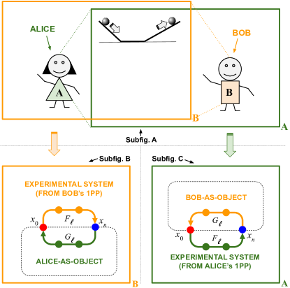
Figure 8: Reflexive coupling between observers: (A; top half) Alice and Bob mutually experience each other, while observing the same experimental system. In this case, Alice and Bob play complementary roles as both the objects being experienced by and the subjects who experience each other (top figure). (B,C) The bottom figures show the corresponding graphical models. Importantly, a change in perspective inverts the sense in which the dynamics flow. Indeed, from Bob’s first-person perspective (1PP), the dynamics of Alice-as-object interacting with the experimental system flow clockwise (B; bottom left). In contrast, from Alice’s 1PP, the dynamics of Bob-as-object interacting with the experimental system flows counter-clockwise (C; bottom right). We refer to this as an “apparent time reversal” (see observer’s property O5 and mirror’s property M5)

So, distinguishing between observer-as-object, $F$, and observer-as-subject, $\text{\sout{$I$}}_{W}$, allows us to stop the infinite regress because we do not need to keep on adding observers-as-objects ad infinitum. However, this step requires us to assume that observers play complementary roles as both subject and object. So, our description is still incomplete because we are taking account of $F$ as an object but not as a subject and of $W$ as a subject but not as an object (see Fig. 7E). We can take full account of these complementary roles that observers play by implementing a reflexive coupling where $F$ and $W$ mutually observe each other interact with the same experimental system $S$ (see Fig. 8 where we use names Alice and Bob instead to emphasize this more symmetric situation).

This is analogous to the situation of two mirrors mutually reflecting both each other and a light bulb. As described in M3, in this situation each mirror also plays complementary roles as the object being reflected by the other mirror and the object-reflecting “subject” that reflects the other mirror. As described in M5, if for one of the two mirrors engaged in a reflexive coupling the object reflected moves with (horizontal) velocity $v$, for the other mirror it moves with velocity $-v$. We have refer to this as an “apparent time reversal.” In the reflexive coupling between two observers there is also an “apparent time-reversal.” Before discussing the implementation of the reflexive coupling, let us discuss in more detail this “apparent time reversal.”

III.3.2 Constraints for a reliable science

In Sec. II.4.6 we argued that if the dynamics external to an embodied observer, Fabienne ($F$), is described by probability matrix $P_{\ell}$ and factors $F_{\ell}$, then the dynamics internal to Fabienne is described by their transposed, i.e., $P_{\ell}^{T}$ and $F_{\ell}^{T}$. This happens because there is an “apparent time reversal” in that the external dynamics flows from $x_{0}$ to $x_{n}$, while the internal dynamics flow from $x_{n}$ to $x_{0}$ (see Fig. 2C). This suggests that when we change from an external or third-person perspective (3PP) into an internal or first-person perspective (1PP) there is an “apparent time reversal” manifested as a transposed operation. Indeed, here we describe a similar “apparent time reversal” that arises when Fabienne and Wigner exchange perspectives, from observer-as-object to observer-as-subject. In doing so, we also point out how the reliability conditions R1-R3 in Sec. I might be incorporated in our framework.

In our relational approach what we consider the experimental system external to Fabienne does not exist in an absolute sense. Rather it is external to Fabienne in the sense that it can be experienced by other observer, Wigner ($W$), different from Fabienne—i.e., $W\neq F$. Figure 8B describes the situation we have been considering till now, wherein Wigner and his friend Fabienne play the role of subject and object, respectively. From Wigner’s 1PP, factors $F_{\ell}$ and $G_{\ell}$, respectively, correspond to Wigner’s experience of the experimental system, which we here denote as $[S]_{W}$, and Wigner’s experience of the physical correlates of Fabienne’s experience of the experimental system, which we denote as $[[S]_{F}]_{W}$—let us denote this situation as $[S]_{W}\sim F_{\ell}$ and $[[S]_{F}]_{W}\sim G_{\ell}$; here $\ell=0,\dotsc,n$.

Figure 8C shows the complementary situation wherein the roles of Wigner and his friend are reversed—i.e., now Wigner is the object being observed by Fabienne-as-subject. The reliability condition R1—standardization—requires that this situation be described in the same manner. That is, we should use the same factors $F_{\ell}$ and $G_{\ell}$. Now, from Fabienne’s 1PP, factors $F_{\ell}$ and $G_{\ell}$, respectively, correspond to Fabienne’s experience of the experimental system, $[S]_{F}$, and Fabienne’s experience of the physical correlates of Wigner’s experience of the experimental system, $[[S]_{W}]_{F}$—in short, $[S]_{F}\sim F_{\ell}$ and $[[S]_{W}]_{F}\sim G_{\ell}$.

The reliability condition R2—intersubjectivity—requires that, at each time step, what Wigner-as-subject considers as the experimental system, $[S]_{W}\sim F_{\ell}$, which is external to his friend, be the same as the experimental system that Wigner-as-object observes via the corresponding physical correlates $[[S]_{W}]_{F}\sim G_{\ell}$. Under an exchange of roles, the initial factor $F_{0}(x_{1},x_{0})$, for instance, characterizing the experimental system observed by Wigner-as-subject (see Fig. 8B), corresponds to the final factor $G_{0}\equiv F_{2n-1}(x_{0},x_{2n-1})$ characterizing the experimental system observed by Wigner-as-object performing the experiment (see Fig. 8C). However, the latter has to be transposed because it corresponds to paths traversed in the reversed direction. More generally, we have

$$G_{\ell}=F_{2n-\ell-1}=F^{T}_{\ell};$$ (68)

which is the same Eq. (41). Here $\ell=0,\dotsc,n$. So, here again the factors $F_{\ell}$ and $G_{\ell}$ are the same, except for the fact that they correspond to paths traversed in reverse directions. Reliability condition R3—truthfulness—requires that if the internal and external dynamics coincide, no observer reports to the contrary.

Importantly, under a change in perspective there is an “apparent time reversal” in that the processes referring to one and the same observer change direction. For instance, when Wigner plays the role of subject, the dynamics of the experimental system experienced by him, $[S]_{W}\sim F_{\ell}$, flows from $x_{0}$ to $x_{n}$. In contrast, when Wigner plays the role of object, the physical processes that refers to him are the physical correlates of his experience, $[[S]_{W}]_{F}\sim F_{\ell}^{T}$, which flow in the opposite direction. This “apparent time-reversal” is characterized by the transposed operation. Let us summarize this as follows:

O5. Observers’ reflexive coupling involves an “apparent time-reversal”: Consider two (sets of) of observers, say $F$ and $W$, engaged in a reflexive coupling. That is, $W$ and $F$ mutually observe each other being engaged in an action-perception loop with an experimental system. Assume that $W$ describes the loop associated to $F$ in a clockwise direction, via changes $\Delta P_{\ell}=\epsilon[J_{s},P_{\ell}]$. Then $F$ describes the loop associated to $W$ in a counter-clockwise direction, via the transposed changes $\Delta P^{T}_{\ell}=-\epsilon[J_{s},P^{T}_{\ell}]$. Alternatively, if $\Delta P^{F}_{\ell}=\epsilon[J_{s},P^{F}_{\ell}]$ are the changes associated to observer $F$, then $\Delta P^{W}_{\ell}=-\epsilon[J_{s},P^{W}_{\ell}]$ are the changes associated to observer $W$. The latter is a less restrictive assumption since the former also requires that $P^{W}_{\ell}=(P_{\ell}^{F})^{T}$. The latter assumption only requires the change $\epsilon\to-\epsilon$ due to the inversion of the temporal labels. Any one of the these two assumptions will be enough for our purposes.

III.3.3 Reflexive coupling and quantum dynamics with stoquastic Hamiltonians

Here we finally describe the reflexive coupling between two observers, $\textsc{Alice}=(\text{\sout{$I$}}_{A},A)$ and $\textsc{Bob}=(\text{\sout{$I$}}_{B},B)$. These new names and new notation highlight that from now on we consider the more symmetric situation wherein each observer plays the two complementary roles as both subject and object.

Intuitively, in line with observer’s property O5, the dynamics of Bob-as-object, as experienced by Alice-as-subject, is the transpose of the dynamics of Alice-as-object, as experienced by Bob-as-subject. The reflexive coupling between Alice and Bob couples these two transposed dynamics via a swap operation analogous to the one that connects Eqs. (48) and (49), which are equivalent to von Neumann equation, into Eqs. (50) and (51), which are formally analogous to the equations describing an embodied observer and its transposed. In this way, the reflexive coupling leads to a dynamics formally analogous to real-time quantum dynamics. However, in this section we are considering the case of symmetric dynamical matrices—i.e., $J_{a}=0$ so $J=J_{s}=J^{T}_{s}$. These correspond to so-called stoquastic Hamiltonians, $H=-\hbar J_{s}$—i.e., Hamiltonians with real, non-positive off-diagonal entries, which can be naturally interpreted in probabilistic terms. We discuss more general Hamiltonians in Sec. III.4 below. We now formalize these ideas.

Embodiment—observer’s property O1—entails that an observer-as-object interacting with an experimental system is described by a real probability matrix $P_{\ell}$ following a dynamics given by Eq. (40). This equation is analogous to that of a single video-feedback-system, Eq. (65), in that they both appear to describe a system on their own, in an absolute, non-relational way.

However, in our relational approach the dynamical changes in one observer-as-object, say Alice-as-object (or $A$), are relative to, or cognized by, another observer-as-subject, say Bob-as-subject (or $\text{\sout{$I$}}_{B}$). To make this explicit, in analogy with video-systems, we will denote this as $\left.\Delta^{\rm e}P_{\ell}^{A}\right|_{B}^{\to}=\epsilon[J_{s},P_{\ell}^{A}]$ (cf. Eq. (40)). Here the superindex “e” emphasizes that these changes are external to Bob—i.e., these are the changes of Alice-as-object described from a 3PP. Furthermore, the arrow $\to$ plays a role analogous to the arrow in Eq. (61), i.e., it emphasizes that this equation is one of a pair describing the reflexive coupling between Alice and Bob. In particular, the arrow $\to$ indicates the situation illustrated in Fig. 8B, where the circular dynamics flows clockwise. A reversed arrow $\leftarrow$ is analogous to the arrow in Eq. (62). That is, it indicates that, like in the case of mirrors (see property M5), there is an “apparent time reversal” when Alice and Bob exchange perspectives (see observer’s property O5)—in other words, it refers to the situation illustrated in Fig. 8C, where the dynamics flows counter-clockwise instead.

Since Bob is also a physical system, there are physical changes internal to him that correlate with his experience of the changes of Alice-as-object, $\left.\Delta^{\rm e}P_{\ell}^{A}\right|_{B}^{\to}$, which are external to him. Such internal physical changes should reflect the external ones. So, these changes should also be described in terms of a real probability matrix $P_{\ell}^{B}$ that describes Bob’s state at time step $\ell$. After experiencing these changes Bob’s state changes to $P_{\ell+1}^{B}=P_{\ell}^{B}+\left.\Delta^{\rm e}P_{\ell}^{A}\right|_{B}$. Importantly, like in the case of video-systems, the first term in the right hand side of this equation is $P_{\ell}^{B}$, not $P_{\ell}^{A}$, because Bob remembers his own previous state not Alice’s. In other words, before Bob experiences the changes $\left.\Delta^{\rm e}P_{\ell}^{A}\right|_{B}^{\to}$, he is in state $P^{B}_{\ell}$. Bob’s experience of the changes of Alice-as-object is supported by physical correlates $\Delta^{\rm i}P_{\ell}^{B}=\left.\Delta^{\rm e}P_{\ell}^{A}\right|_{B}^{\to}$—here the superindex “i” emphasizes that these changes are internal to Bob-as-subject. So, in analogy with mirror property M1, we introduce the following observer’s property:

O6. Embodied observers experience objects via physical changes—internal and external: In between any two time steps, $\ell$ and $\ell+1$, the change in state of an observer-as-object, $A$, interacting with an experimental system, as experienced by an observer-as-subject,  $\text{\sout{$I$}}_{B}$, is given by

$$\left.{\Delta^{\rm e}P_{\ell}^{A}}\right|_{B}^{\to}=\epsilon[J_{s},P_{\ell}^{A}].$$ (69)

These changes, which are external to $\text{\sout{$I$}}_{B}$ (as emphasized by superindex “e”), induce changes $\Delta^{\rm i}P_{\ell}^{B}$, which are internal to $\text{\sout{$I$}}_{B}$ (as emphasized by superindex “i”) and correlate with $\text{\sout{$I$}}_{B}$’s experience of observing those external changes. That is (cf. Eq. (55) and (66))

$$\Delta^{\rm i}P_{\ell}^{B}=\left.{\Delta^{\rm e}P_{\ell}^{A}}\right|_{B}^{\to},$$ (70)

In other words, since observer $\textsc{Bob}=(B,\text{\sout{$I$}}_{B})$ is itself a physical system there are physical changes, $\Delta^{\rm i}P^{B}_{\ell}$, implicit or unobservable to Bob that allows him to experience the observer-as-object  $A$.

Equation (70) ignores the role of Alice-as-subject as well as the role of Bob-as-object. We can take account of Alice’s and Bob’s complementary roles as both subject and object, without introducing any new observers, by implementing a reflexive coupling between them. In this way, Alice’s and Bob’s descriptions are relative to each other, rather than to an unacknowledged external observer. As discussed in Sec. III.3.1, introducing such an external observer would require us to introduce yet another observer that observes the former, which would result in an infinite regress.

To implement the reflexive coupling, we have to consider the case where Alice and Bob play the complementary roles of the subject who observes and the object being observed, respectively. In analogy with Eq. (70), this yields the equation $\Delta^{\rm i}P_{\ell}^{A}=\left.{\Delta^{\rm e}P_{\ell}^{B}}\right|_{A}^{\leftarrow}$. This equation is the analogue of Eq. (62) for mirrors. Again, the reverse arrow $\leftarrow$ indicates that there is an “apparent time reversal” (see observer’s property O5 and Figs. 8C; cf. the analogous mirror’s property M5). So, we introduce the following observer’s property:

O7. Reflexivity: To describe the world from within, without any reference to external observers, two (sets of) observers must implement a reflexive coupling where they mutually observe each other. In analogy with Eqs. (61) and (62), this is described by the pair of equations:

$$\Delta^{\rm i}P^{A}_{\ell} = \left.{\Delta^{\rm e}P^{B}_{\ell}}\right|_{A}^{\leftarrow},$$ (71)

$$\Delta^{\rm i}P^{B}_{\ell} = \left.{\Delta^{\rm e}P^{A}_{\ell}}\right|_{B}^{\to}.$$ (72)

So, the reflexive coupling implements a swap operation analogous to the one that turned Eqs. (48) and (49), which are equivalent to von Neumann equation, into Eqs. (50) and (51), which are formally analogous to the equations describing an embodied observer and its transposed—again, in this section we are considering the case of symmetric dynamical matrices, i.e., $J_{a}=0$ so $J=J_{s}=J^{T}_{s}$.

We will now explore in what sense Eqs. (71) and (72) are indeed formally analogous to von Neumann equation. To begin, the right hand side of Eq. (72), which is given by Eq. (69), describes a situation analogous to that illustrated in Fig. 8B, where Alice and Bob, respectively, play the role of object (like $F$ in Fig. 7E), and subject (like $W$ in Fig. 7E). With this convention, the right hand side of Eq. (71), $\left.\Delta P^{B}_{\ell}\right|_{A}^{\leftarrow}$, describes the complementary situation shown in Fig. 8C, where the roles of Alice and Bob are reversed. According to observer’s property O5, an exchange of roles entails an “apparent time reversal”, which manifests in the change $\epsilon\to-\epsilon$. That is,

$$\left.\Delta^{\rm e}P^{B}_{\ell}\right|_{A}^{\leftarrow}=-\epsilon\left[J_{s},P_{\ell}^{B}\right].$$ (73)

So, Eqs. (71) and (72) can be written as

$$P^{A}_{\ell+1} = P^{A}_{\ell}-\epsilon\left[J_{s},P^{B}\right],$$ (74)

$$P^{B}_{\ell+1} = P^{B}_{\ell}+\epsilon\left[J_{s},P^{A}_{\ell}\right].$$ (75)

If we can show that $P^{A}_{\ell}=(P^{B}_{\ell})^{T}=P_{\ell}$, for all $\ell$, then Eqs. (74) and (75) become $\Delta P_{\ell}=-\epsilon[J_{s},P_{\ell}^{T}]$ and $\Delta P_{\ell}^{T}=\epsilon[J_{s},P_{\ell}]$, respectively, which are equivalent to Eqs. (48) and (49) (again, with $J_{a}=0$), which are in turn formally analogous to von Neumann equation, Eq. (20). So, all that we need to show is that $P^{A}_{\ell}=(P^{B}_{\ell})^{T}$, for all $\ell$.

We will start with the base case, i.e.,

$$P_{0}^{A}=(P_{0}^{B})^{T}.$$ (76)

Indeed, according to Eqs. (42), the initial state of the dynamics of an embodied scientist is given by $P_{0}=\widetilde{F}_{n}\widetilde{F}_{n}^{T}=P_{0}^{T}$, which is symmetric. Since factors $F_{\ell}$ are the same for Alice and Bob (up to a transpose operation), it seems natural to assume that they have the same initial symmetric state $P_{0}^{A}=P_{0}=P_{0}^{T}=P_{0}^{B}$, in which case they are trivially related by a transpose operation. We summarize this in the following observer’s property:

O8. The initial states of two reflexively coupled observers is the same and symmetric: This is given by $P_{0}=\widetilde{F}_{n}\widetilde{F}_{n}^{T}=P_{0}^{T}$, which implies that the states of the two observers, Alice and Bob, are trivially related by a transposed operation, i.e., $P_{0}^{A}=P_{0}=P_{0}^{T}=P_{0}^{B}$—so, Eq. (76) is naturally satisfied. We will discuss the case of more general initial states in Sec. III.5 below.

We now show that with the base case expressed in Eq. (76) we have that $P_{\ell}^{A}=(P_{\ell}^{B})^{T}$, for all $\ell$, and so Eqs. (71) and (72) are formally analogous to von Neumann equation, Eq. (20). We will show this by induction, i.e., by showing that if $P_{\ell}^{A}=(P_{\ell}^{B})^{T}$ at time step $\ell$ then $P_{\ell+1}^{A}=(P_{\ell+1}^{B})^{T}$ at time step $\ell+1$. We already have the base case for $\ell=0$, as expressed in Eq. (76). So, let us assume that $P_{\ell}^{A}=(P_{\ell}^{B})^{T}$ at a generic time step $\ell$. Taking the transpose of Eq. (74) yields $(P^{A}_{\ell+1})^{T}=(P^{A}_{\ell})^{T}+[J_{s},(P^{B}_{\ell})^{T}]$ since $J_{s}=J_{s}^{T}$ is symmetric. This equation can be written as

$$(P^{A}_{\ell+1})^{T}=P^{B}_{\ell}+[J_{s},P^{A}_{\ell}],$$ (77)

since $(P_{\ell}^{A})^{T}=P_{\ell}^{B}$. Now, the right hand side of Eq. (77) equals the right hand side of Eq. (74). Therefore, the left hand sides of those same equations should be equal, i.e., $P_{\ell+1}^{B}=(P_{\ell+1}^{A})^{T}$. Thus, Eq. (74) is the transposed of Eq. (75) as we wanted to show.

Alternatively, we can obtain the same result if we assume that an “apparent time reversal” manifests as a transposed operation as discussed in observer’s property O5. In this way, Eq. (73) can be replaced with the equation

$$\left.\Delta^{\rm e}P^{B}_{\ell}\right|_{A}^{\leftarrow}=\left(\left.\Delta^{\rm e}P^{A}_{\ell}\right|_{B}^{\to}\right)^{T}=-\epsilon\left[J_{s},\left(P_{\ell}^{A}\right)^{T}\right].$$ (78)

It can be shown along the same lines that, under the condition expressed in Eq. (76), Eqs. (78) and (72) are also equivalent to von Neumann equation, Eq. (20).

So, this shows that the reflexive coupling between two embodied observers can entail a dynamics formally analogous to real-time quantum dynamics with an initial state given by a density matrix that is real, symmetric and has non-negative entries. We will discuss in Sec. III.5 below the situation of more general density matrices.

However, there is a technical assumption in the reflexive coupling that we now make more explicit. Equations (74) and (75) build on Eq. (40), describing the dynamics of an observer-as-object from the perspective of an observer-as-subject. However, Eqs. (74) and (75) entail a dynamics which is different, in general, to the dynamics entailed by Eq. (40). So, at time step $\ell$, the probability matrix $P_{\ell}$ entailed by Eqs. (74) and (75) can in principle be outside the domain of the dynamics described by Eq. (40)—e.g., $P_{\ell}$ might have negative off-diagonal entries due to the minus sign associated to the “apparent time reversal.”

So, we are implicitly assuming that Eq. (40) connects the dynamics in between any two consecutive time steps, even in such more general cases. That is, we have to relax the constrain that the off-diagonal elements have to be non-negative, while keeping the constraint that the diagonal elements are probabilities. This is somewhat analogous to one of the postulates Feynman used to derive his path-integral formulation of quantum mechanics. That is, that in between two consecutive time steps all paths are characterized by the corresponding classical action, even though most of those paths may not be the ones that a classical particle would follow. In our case, in between two consecutive time steps observers are characterized by the dynamics that an observer-as-object would follow, as described by another observer-as-subject, even though this is not the actual dynamics that observers follow after the reflexive coupling is made. The fact that, after a reflexive coupling, the diagonal of the probability matrices involved still represent probabilistic information suggests that an integrated approach that couples from the start both embodiment and reflexivity may help better formalize these ideas.

III.4 Quantum dynamics with more general Hamiltonians

Our discussion up to now has been restricted to symmetric dynamical matrices $J_{s}$ with non-negative off-diagonal entries, which can be interpreted in probabilistic terms via the corresponding factors $F_{\ell}={\rm 1\!\!I}+\epsilon J_{s}+O(\epsilon^{2})$. So, we have only considered real Hamiltonians, $H_{s}=-{\Gamma}J_{s}$, with non-positive off-diagonal entries (see Eq. (45))—here ${\Gamma}$ is the analogue of Planck constant. Genuine quantum dynamics does not seem to have this restriction, though, since general Hamiltonians, $H=H_{s}+H_{a}/i$, can also have positive and complex entries which, according to Eq. (45), can entail asymmetric dynamical matrices with negative entries, $J=-H_{s}/{\Gamma}-H_{a}/{\Gamma}$—here $H_{s}$ and $H_{a}$ are symmetric and anti-symmetric operators, respectively.

We now discuss how our approach can accommodate this more general situation. We do this from two different perspectives. First, we discuss a couple of examples to show that effective asymmetric dynamical matrices with off-diagonal negative entries can arise from approximations of systems described by symmetric dynamical matrices with non-negative off-diagonal entries. Second, we motivate the introduction of the last observer’s property which enables us to extend our results to dynamical matrices with a non-zero anti-symmetric part.

III.4.1 Effective non-stoquastic Hamiltonians as approximations of stoquastic ones

To begin, consider the well-known case of a (two-dimensional) two-level atom which arises after truncating the full (infinite dimensional) model of an atom interacting with a coherent radiation field haken2005physics (see Sec. 15.3 therein; see Appendix D herein). The full model consists of an electron, described by the momentum operator $i\hbar\nabla_{\mathbf{x}}$, moving in a potential $V(\mathbf{x})$ produced by the nucleus—here $\mathbf{x}$ and $\nabla_{\mathbf{x}}$ are the three-dimensional position vector and differential operator, respectively. So, the free atom—without the coherent radiation field—is characterized by the Hamiltonian

$$H_{0}=-\frac{\hbar^{2}}{2m}\nabla^{2}_{\mathbf{x}}+V(\mathbf{x})=\sum_{n=0}^{\infty}E_{n}\left|n\rangle\langle n\right|$$ (79)

The expression after the first equality is the three-dimensional version of Eq. (13). So, this example can be handled completely with the tools we have developed up to now. The coherent radiation field is characterized by a time-dependent potential energy $U(\mathbf{x},t)=\mathbf{r}\cdot\mathbf{D_{0}}\cos(\omega t)$, considered as a perturbation to $H_{0}$—here $\mathbf{D_{0}}$ is a suitable constant vector and $\omega$ is the frequency at which the coherent radiation field oscillates. The perturbed model can still be handled completely with the tools we have developed up to now by simply replacing $V(\mathbf{x})$ in Eq. (79) with $V(\mathbf{x})+U(\mathbf{x},t)$.

The expression after the second equality in Eq. (79) is the expansion in the eigenbasis of $H_{0}$. The two-level atom is obtained by assuming that the coherent radiation field is near resonance with two relevant energy levels—say, $E_{0}$ and $E_{1}$. Under this assumption we can keep only two terms in the series after the second equality in Eq. (79) and handle the coherent radiation field as a perturbation. The two-level atom so obtained is described by an effective Hamiltonian

$$H_{\rm eff}=\overline{E}{\rm 1\!\!I}_{2}-C\sigma_{Z}+D\cos(\omega t)\sigma_{X},$$ (80)

where $\overline{E}$, $C$, and $D$ are suitable constants, and ${\rm 1\!\!I}_{2}=\left|0\rangle\langle 0\right|+\left|1\rangle\langle 1\right|$, $\sigma_{Z}=\left|0\rangle\langle 0\right|-\left|1\rangle\langle 1\right|$ and $\sigma_{X}=\left|0\rangle\langle 1\right|+\left|1\rangle\langle 0\right|$, respectively, are the two-dimensional identity matrix, the Pauli matrix in the $Z$ direction, which is diagonal, and the Pauli matrix in the $X$ direction, which has zeros in the diagonal and ones in the off-diagonal. The factor $\cos(\omega t)$ multiplying $\sigma_{X}$ can have positive and negative values, depending on the value of $t$. So, the effective Hamiltonian described in Eq. (80) can have both negative and positive off-diagonal entries, even though the original Hamiltonian $H_{0}+U$ from which it is derived only has negative off-diagonal entries, given by the first term after the first equality in Eq. (79).

Now consider the case of more general complex Hamiltonians, $H_{\ell}=H_{s,\ell}+H_{a,\ell}/i$, which are associated to asymmetric dynamical matrices $J_{\ell}=J_{s,\ell}+J_{a,\ell}$ (see Eq. (45)). There are also examples where these kinds of Hamiltonians with complex entries can be obtained as approximations to real Hamiltonians with non-positive entries. For instance, Vinci and Lidar discuss the case of superconducting flux qubits described by a real Hamiltonian with non-positive off-diagonal entries given by a kinetic term of the form $-(E_{C}/2)\sum_{j}\partial^{2}/\partial\phi^{2}_{j}$, where $\phi_{j}$ refer to the magnetic fluxes trapped by the flux qubits, and $E_{C}$ represents a charging energy vinci2017non (see Eq. (1) therein). After some approximations Vinci and Lidar obtain an effective Hamiltonian that has a purely imaginary term, even though the original Hamiltonian is real and has non-positive off-diagonal entries vinci2017non (see Eq. (11) therein).

This invites the question of whether general Hamiltonians can be obtained as approximations of real Hamiltonians with non-positive entries, which can be accommodated in our approach. Trying to answer this question might help us better understand what is fundamental in quantum theory and what is simply approximation methods. Anyways, we now discuss the final observer’s property, which will enable us to obtain a class of Hamiltonians with complex entries.

III.4.2 Observers only experience relative changes

Now consider the case of a free particle given by the real Hamiltonian in Eq. (13) with $V=0$. This yields the Schrödinger equation

$$i\hbar\frac{\partial\psi}{\partial t}=-\frac{\hbar^{2}}{2m}\frac{\partial^{2}\psi}{\partial x^{2}},$$ (81)

whose classical analogue is the diffusion equation with zero drift, i.e., $\partial p/\partial x=D\partial^{2}p/\partial x^{2}$. Equation (81) acquires an imaginary part if we change to a reference frame moving with velocity $v$ padmanabhan2011nonrelativistic (see Eqs. (14)-(16) therein)

$$i\hbar\frac{\partial\psi}{\partial t}=-\frac{\hbar^{2}}{2m}\frac{\partial^{2}\psi}{\partial x^{2}}+i\hbar v\frac{\partial\psi}{\partial x}.$$ (82)

This is because the time derivative accordingly changes as $\partial/\partial t\to\partial/\partial t+v\partial/\partial x$, and the time derivative is multiplied by $i$. The classical analogue of this is a diffusion equation with non-zero drift $\partial p/\partial x=D\partial^{2}p/\partial x^{2}-v\partial p/\partial x$. Of course, the new term in Eq. (82) can be canceled by introducing the rule that the wave function also has to be multiplied by a suitable phase under a change of reference frame padmanabhan2011nonrelativistic (see Eqs. (21) and (22) therein). However, refraining from introducing this rule will help us illustrate the point we want to make.

So, the new Hamiltonian in the moving reference frame is $H_{\ell}=H_{s,\ell}+H_{a,\ell}/i$, with $H_{s,\ell}=-(\hbar^{2}/2m)\partial^{2}/\partial x^{2}$ and $H_{a,\ell}=\hbar v\partial/\partial x$, which according to Eqs. (48) and (49) yields

$$\Delta P_{\ell}-\epsilon[J_{a,\ell},P_{\ell}] = -\epsilon[J_{s,\ell},P^{T}_{\ell}],$$ (83)

$$\Delta P^{T}_{\ell}-\epsilon[J_{a,\ell},P^{T}_{\ell}] = \epsilon[J_{s,\ell},P_{\ell}],$$ (84)

where we have moved the term containing $J_{a,\ell}$ to the left hand side. Here $J_{s,\ell}=-H_{s,\ell}/\hbar$, $J_{a,\ell}=-H_{a,\ell}/\hbar$, and $\rho_{\ell}=(P_{\ell}+P_{\ell}^{T})/2+(P_{\ell}-P_{\ell}^{T})/2i$.

This situation is analogous to mirror’s property M6 since the anti-symmetric term here arises from a change of reference frame. The commutators in the left-hand side of Eqs. (83) and (84) could be considered as removing the motion common to the two observers in the reflexive coupling as well as to the object being observed. In this sense they are analogous to the term $v_{C|W}$ in Eqs. (63) and (64). We can capture this intuition in the following observer’s property (see mirror’s property M6):

O9. Observers involved in a reflexive coupling can only experience relative changes: Two (sets of) observers involved in a reflexive coupling cannot observe the part characterized by $J_{a,\ell}$, since this only exists relative to an observer external to them. So, when performing the reflexive coupling associated to a general dynamical matrix $J_{\ell}=J_{s,\ell}+J_{a,\ell}$, we first have to subtract the anti-symmetric part, precisely as in Eqs. (83) and (84).

Observer’s property O9 leads to the analogue of von Neumann equation with a class of non-stoquastic Hamiltonians with complex entries. For instance, consider the real Hamiltonian-like function

$$\mathcal{H}_{\rm EM}(\mathbf{x},\mathbf{x}^{\prime})=\frac{m}{2}\left(\frac{\mathbf{x}-\mathbf{x}^{\prime}}{\epsilon}\right)^{2}+V\left(\frac{\mathbf{x}+\mathbf{x}^{\prime}}{2},t\right)+\frac{e}{c}\left(\frac{\mathbf{x}-\mathbf{x}^{\prime}}{\epsilon}\right)\cdot\mathbf{A}\left(\frac{\mathbf{x}+\mathbf{x}^{\prime}}{2},t\right)+\frac{e^{2}}{mc^{2}}\left[\mathbf{A}\left(\frac{\mathbf{x}+\mathbf{x}^{\prime}}{2},t\right)\right]^{2}.$$ (85)

This leads to factors with an anti-symmetric component due to the third term in the right hand side, which is linear in $\mathbf{x}-\mathbf{x}^{\prime}$. Dealing with this anti-symmetric component according to observer’s property O9 leads to the Schrödinger equation of a quantum particle in an electromagentic field $\mathbf{A}$, i.e.,

$$\begin{split}i\hbar\frac{\partial\psi(\mathbf{x},t)}{\partial t}=&-\frac{\hbar^{2}}{2m}\left(\nabla-i\frac{e}{\hbar c}\mathbf{A}\right)^{2}\psi(\mathbf{x},t)\\ &+eV(\mathbf{x},t)\psi(\mathbf{x},t).\end{split}$$ (86)

We show this in Appendix A.

III.5 Generic initial quantum states and observables

Here we show how the previous results can be extended to more general initial density matrices and observables. In our approach the initial density matrix is given by $\rho_{0}=P_{0}=\widetilde{F}_{n}\widetilde{F}_{n}^{T}$, which is real and so symmetric. This is not necessarily a restriction, though. More general “initial” quantum states $\rho_{\rm prep}=U_{\rm prep}\rho_{0}U_{\rm prep}^{\dagger}$ can be prepared after applying a suitable quantum operation $U_{\rm prep}$ to $\rho_{0}$. In principle, we can write $U_{\rm prep}=U_{m}\cdots U_{0}$, for a suitable number of time steps $m$, where each $U_{\ell}={\rm 1\!\!I}-i\epsilon H_{\ell}/{\Gamma}$ is obtained from a factor $F_{\ell}={\rm 1\!\!I}+\epsilon J_{\ell}$ via $H_{\ell}=-{\Gamma}(J_{s,\ell}+J_{a,\ell}/i)$—here $\ell=0,\dotsc,m$.

Furthermore, we have mostly focused on one observable, i.e., position. However, according to Feynmann “all measurements of quantum-mechanical systems could be made to reduce eventually to position and time measurements (e.g., the position of the needle on a meter or the time of flight of a particle). Because of this possibility a theory formulated in terms of position measurements is complete enough in principle to describe all phenomena” feynman2010quantum (p. 96).

Indeed, this view aligns with our focus on modeling how science is actually performed in practice and how concepts are constructed out of this. For instance, the concept of momentum $p=-i\hbar\partial/\partial x$ of a particle is usually taken as existing in an abstract space. However, to actually measure momentum in practice we need to make the focus system interact with another system that serves as a measuring device. The measuring device can be the position $X$ of a probe particle that interacts with the focus system.

The concept of momentum can emerge out of the description of what actually happens in practice while measuring it. Indeed, let the initial state of the probe be a Gaussian, $\psi_{\rm dev}(X)\propto e^{-X^{2}/4\sigma^{2}}$, centered around zero, with $0<\sigma\ll 1$ characterizing the initial uncertainty on the probe’s position. Since $e^{ikx}$ are eigenfunctions of the momentum operator, with eigenvalues $\hbar k$, it is convenient to write the initial state of the system as $\psi_{\rm sys}(x)\propto\int c_{k}e^{ikx}\mathrm{d}k$, where $c_{k}$ are suitable coefficients. After a suitable interaction between the two particles, we can obtain the joint state $\Psi(x,X)\propto\int c_{k}e^{ikx}e^{-(X-a\hbar k)^{2}/4\sigma^{2}}\mathrm{d}x$, where $a$ is a constant, and the corresponding joint probability $\mathcal{P}(x,X)=|\Psi(x,X)|^{2}$ aharonov2008quantum (ch. 7-9).

However, in practice we are not interested in observing $x$, but on inferring the momentum of the system by observing only the probe. Marginalizing $x$ yields $\mathcal{P}_{\rm dev}(X)\approx\int{|c_{k}|^{2}}\delta(X-a\hbar k)\mathrm{d}k$ for $\sigma\ll 1$, where $\delta$ is the Dirac delta function. Thus with probability $\propto\,|c_{k}|^{2}$ the position of the probe, $X=a\hbar k$, is proportional to the momentum eigenstate $\hbar k$. This is the (projective) measurement postulate of quantum theory.

IV Discussion

So, how can scientists escape the action-perception loop and establish an observer-independent science? Our results suggest that scientists appear to do this by describing the world with the tools of quantum theory. This gives the impression that scientists can actually obtain an observer-independent description of the world—a world that just happens to be quantum for no reason. However, our results suggest that there is indeed a reason for why scientists have to use the tools of quantum theory: to effectively account for the observer and the experimental context.

This aligns with growing evidence suggesting that in quantum theory facts are relative brukner2020facts . Indeed, our approach shares some elements with the main interpretations of quantum theory that endorse relative facts Rovelli-1996 ; mermin2014physics ; debrota2018faqbism ; fuchs2013quantum ; pienaar2021qbism ; brukner2017quantum : Like QBism, our approach explicitly acknowledges the role of scientists in science mermin2014physics ; fuchs2013quantum ; debrota2018faqbism ; pienaar2021qbism . Like the (neo-)Copenhagen interpretation of quantum theory brukner2017quantum , our approach explicitly acknowledges the experimental context. Like RQM Rovelli-1996 ; rovelli2021helgoland , our approach acknowledges that the relation “an observer observes a phenomenon” is itself relative to another observer.

However, there are important differences too. To begin, QBism treats scientists as rather abstract agents immersed in a publicly shared physical universe. The quantum formalism is seen as a normative criterion debrota2018faqbism (see Sec. 18 therein) setting “the standard to which agents should strive to hold their expectations”. Such agents are betting, implicitly or explicitly, on their subsequent experiences, based on earlier ones, and the quantum formalism is a tool to help them place better bets mermin2018making (p. 8). Rovelli recently criticized QBism because it “sees the world reflected in the observer,” instead of seeing the observer as a part of the world rovelli2021helgoland (p. 68-69). For Rovelli, the crucial point that QBism disregards is that the observer himself can be observed. Rovelli is concerned that QBism “leaves behind naive materialism but ends up falling into an implicit form of idealism” rovelli2021helgoland (p. 69). However, unlike us, Rovelli treats observers as generic quantum systems—that is, as far as physics is concerned, for Rovelli there are no relevant differences between an electron and an observer.

Our approach suggests a middle way between QBism and RQM since we treat observers as physical systems with a dynamical role to play, but not as any kind of physical system. Instead of working with an abstract notion of what physicists might assume an observer is, however, our approach builds on general insights gained by the area of science dedicated to investigate actual observers, i.e., cognitive science. Moreover, we do not treat observers as quantum systems, but as classical cognitive systems. Importantly, non-trivial aspects of the quantum formalism emerge out of two key concepts: embodiment and reflexivity (see below). To clarify, observers can be described by other observers as quantum systems since they are physical systems too. However, our approach suggests that this is due to the relationalism between classical observers and classical experimental systems, which manifests as embodiment and reflexivity.

Our results suggests that the kind of relationalism associated to quantum theory is the circular co-dependence between perceiver and world, which, according to Varela et al. varela2017embodied (p. 172), allows embodied cognition to find a middle way between materialism and idealism. Indeed, in this approach neither the perceiver nor the world are primary, but they depend on each other like “two sheaves of reeds propping each other up.” More precisely, the kind of relationalism associated to our approach entails a double circularity, one associated to embodiment and another to reflexivity (see below)—a kind of “strange loop” hofstadter2013strange . In contrast, Rovelli conceives relationalism in terms of a generic network of relations, not in terms of circularity.

Our results suggest that the core message of quantum theory might be summarized in two core principles: (i) Observers are embodied; this is associated to observer’s property O1. (ii) The world must be described from within—that is, without any reference to external observers; this is effectively associated to observer’s properties O2-O9. Principles (i) and (ii) entail embodiment and reflexivity, respectively. Here embodiment refers to the idea that when scientists interact with an experimental system they are involved in an instrumentally-mediated action-perception loop (see Figs. 1B, 2A). Reflexivity refers to the idea that for scientists to describe the world without any reference to external observers, two (sets of) observers should mutually describe each other (see Fig. 8). Embodiment and reflexivity are rather generic concepts, and our model is rather minimal. So, our approach should not be restricted to a specific kind of observer.

As we said, in line with RQM, we assume that a scientist, say Fabienne, doing an experiment does not exist in an absolute sense, but she is relative to another external observer, say Wigner. In this case Fabienne plays the role of an object being observed by Wigner—this additional observer is typically neglected in cognitive science. Now, to be consistent, we should also take into account the observer that observes Wigner. Otherwise, Wigner would exist in an absolute, non-relational way. So, who does observe Wigner? If we added another observer, say Rovelli, so that Wigner becomes an object of observation for Rovelli, we would be headed into an infinite regress. Indeed, we can now ask: who does observe Rovelli? And so on.

We escaped this infinite regress in two steps. First, we assumed that observers play two complementary roles: as objects being observed by other observers and as “subjects” that can observe other objects, including other observers (see Fig. 7E). Here “subject” is used in the strict technical sense of the opposite of object, or not-an-object. For instance, in the example above Fabienne plays the role of an object for Wigner, but Wigner plays the role of a subject for himself in the sense that Wigner cannot completely become an object of observation for himself. This is analogous to a mirror that cannot directly reflect itself—though it can do so indirectly with the help of another mirror. Acknowledging that Wigner cannot become an object of observation for himself stops the chain of infinite regress since we do not need to keep on adding observers-as-objects ad infinitum. We acknowledge that there is something that cannot become an object of observation, a “subject.”

This may be a subtle point, so let us discuss it a bit more. Please imagine, for instance, that you observe a physical system $S$. Besides $S$, which is external to you, there are physical processes inside you that allow you to experience $S$, e.g., the neural correlates associated to your experience of $S$—denoted here as $\{S\}$. For $S$ and $\{S\}$ to be correlated, there has to be a physical interaction between them. Such a physical interaction may or may not be negligible; however, we do not want to a priori neglect it, but to determine a posteriori whether we can do so. While $\{S\}$ is key in allowing you to experience $S$, it is absent for you in the sense that you cannot simultaneously and directly experience both $S$ and $\{S\}$ as objects of observation. If you simultaneously and directly observe both $S$ and $\{S\}$ you are observing a different physical object, i.e., $S+\{S\}$, with associated physical correlates $\{S+\{S\}\}$, which you cannot directly observe at the same time that you observe $S+\{S\}$. Again, this is the analogue of a mirror that cannot directly reflect itself.

Now, when you play the role of a subject that observes a system $S$, you describe $S$ from your own first-person perspective (1PP)—you can refer to this as “I observe $S$.” In contrast, when somebody else observes you, while you observe $S$, you play the role of an object, you are being described from a third-person perspective (3PP)—the other observer can refer to you as “he observes $S$.” In analogy with this, we denoted an observer-as-subject, say Wigner, as $\text{\sout{$I$}}_{W}$. Here the symbol $I_{W}$ refers to Wigner’s 1PP, while the cancellation refers to its “absential nature” to use an expression by Deacon deacon2011incomplete (ch. 0)—this cancellation is inspired in Heidegger sous erasure. Here $\text{\sout{$I$}}_{W}$ is similar to the number zero in that it is a placeholder to indicate the absence of something.

Due to this “absential nature” we cannot directly access the degrees of freedom of the physical correlates of $\text{\sout{$I$}}_{W}$. So, we model such physical correlates indirectly in the same way that we model the inaccessible degrees of freedom of a thermal bath, i.e., as fluctuations or noise characterized by a temperature- or diffusion-like constant, ${\Gamma}$, which turned out to be the analogue Planck’s constant, $\hbar$. Such fluctuations are all-pervasive and irreducible since $\text{\sout{$I$}}_{W}$ is always present whenever an object is being observed and cannot be reduced to an object of observation like, e.g., the atoms of a thermal bath. These properties are analogous to the properties of actual quantum fluctuations, which are also all-pervasive and irreducible. If it turns out that ${\Gamma}=\hbar$, the bar in $\hbar$ could remind us of the “absential nature” of observers-as-subjects.

Here we built on an analogy with Thompson’s neurophenomenological perspective thompson2014waking which distinguish between contents of experience and experience as such—i.e., the mere capacity to experience any content at all from a first-person perspective (1PP). For Thompson, while contents of experience are objects of observation, experience as such cannot become an object of observation because it is the very precondition to experience any object at all—it is like an eye that can see objects in the visual field, but cannot see itself. In line with this, we distinguish between the physical correlates $[[S]]$, that allows a subject, say Wigner, to discriminate between $S$ and any other system $S^{\prime}\neq S$, and the physical correlates associated to the mere capacity to experience any system at all, which we refer to as $[[\text{\sout{$I$}}_{W}]]$ (see below). So, here $\{S\}=[[S]]+[[\text{\sout{$I$}}_{W}]]$. Clearly, $[[S]]$ can be inferred from $S$ because they both refer to the same object. In contrast $[[\text{\sout{$I$}}_{W}]]$ refers to the mere capacity to experience from a 1PP, not to any specific system. In line with Thompson, we assumed $[[\text{\sout{$I$}}_{W}]]$ to be fundamentally inaccessible to Wigner, and thus modeled it as noise.

Anyways, coming back to our previous discussion of Fabienne and Wigner, assuming that Wigner plays the role of a subject and Fabienne that of an object allows us to stop the infinite regress. However, the description is still incomplete because we are neglecting the role of Wigner as object and that of Fabienne as subject. This brings us to the second step to escape the infinite regress. We have to implement a reflexive coupling between Fabienne and Wigner where they play both roles as the subjects that observe each other from a 1PP, and the objects being observed by each other from a 3PP. So, while embodiment implements a kind of circular relationalism between observers-as-object and experimental system, reflexivity implements a kind of circular relationalism between between subject and object, between the 1PP and the 3PP. We could summarize this by saying that every experience has a physical correlate and that every physical phenomenon is an experience for someone—this does not imply that rocks have experiences, but that rocks are rocks for someone who experience them as such. This is analogous to what is sometimes referred to in the literature as “subject-object non-duality” thompson2014waking ; tang2015neuroscience —i.e., the interdependence between subject and object.

The prospects of a science that depends on the observer may be seen as something negative. However, we believe this possibility could also be seen in a positive light. To begin, if taking explicit account of the observer can entail the formalism of quantum theory, as our results suggest, this means that an observer-dependent science does not have to violate current scientific knowledge. It would only violate our assumption that we have the special status of understanding the world from a disembodied perspective, independent of our capacity to experience it, as if we were not part of the world. Indeed, we might learn something useful by rigorously investigating whether indeed we have this special status in the same way that our understanding of the universe advanced when we doubted our special status of being at the center of it.

Furthermore, the prospects of an observer-dependent science suggest a potential relationship between quantum physics and the areas of science that rigorously investigate observers, such as cognitive science and neurophenomenology. In particular, if the quantum formalism—the foundation on which the skyscraper of science stands—already integrates subject and object, the 1PP and the 3PP, the question of how subjective experience “emerges” out of physics might become more tractable. What would emerge is not experience as such but increasingly complex contents of experience. This would parallel the emergence of increasingly complex physical phenomena from the “basic constituents of matter.” Importantly, this also suggests new kinds of experiments, where the objective and subjective aspects of the observer can be part of the experimental setup. For instance, rigorous mind training techniques may allow scientists to directly experience, from a 1PP, the relational nature of the world. There have been reports about this even before the advent of science as we know it. We will discuss this and other potential links between our work and the philosophy of mind elsewhere.

Data availability: Data sharing not applicable to this article as no datasets were generated or analysed during the current study.

Appendix A Particle in an electromagnetic field via real non-negative kernels

Here we discuss the case of a quantum particle in a classical electromagnetic field, which is associated to a complex (and so non-stoquastic) Hamiltonian operator. We show that this can also be written in terms of non-negative real kernels. This adds further evidence that the non-negativity of the factors in our approach does not necessarily restrict it to stoquastic Hamiltonians.

The Schrödinger equation of a particle of charge $e$ interacting with an electromagnetic field can be written as

$$\begin{split}i\hbar\frac{\partial\psi(\mathbf{x},t)}{\partial t}=&-\frac{\hbar^{2}}{2m}\left(\nabla-i\frac{e}{\hbar c}\mathbf{A}\right)^{2}\psi(\mathbf{x},t)\\ &+eV(\mathbf{x},t)\psi(\mathbf{x},t),\\ \end{split}$$ (87)

where $\mathbf{x}$ denotes the position vector in three dimensional space, while $V$ and $\mathbf{A}$ denote the scalar and vector fields respectively. Notice that the Hamiltonian associated to Eq. (87) now contains an imaginary part given by the terms linear in $\mathbf{A}$ arising from the expansion of ${(\nabla-ie\mathbf{A}/\hbar c)^{2}\psi(\mathbf{x},t)}$.

We will show in a series of three theorems and a corollary that Eq. (87) can be written as a pair of equations analogous to Eqs. (48) and (49) in the main text with a non-negative real kernel. As we discussed in the main text, these pair of equations are equivalent to von Neumann equation.

In the first theorem and corollary, we show that Eq. (87) and the corresponding von Neumann equation can be written in terms of convolutions with a complex-valued kernel $\mathcal{C}\propto e^{-\epsilon\widetilde{\mathcal{H}}_{EM}/\hbar}$, where $\widetilde{\mathcal{H}}_{EM}$ is a complex-valued Hamiltonian-like function. Afterwards, in the second theorem, we show that $\mathcal{C}$ can be replaced by a real-valued kernel $\mathcal{W}\propto e^{-\epsilon\mathcal{Q}_{EM}/\hbar}$ in the limit when $\epsilon\to 0$. However, $\mathcal{Q}_{EM}$ depends on $\hbar$, unlike the Hamiltonian-like function in Eq. (1) in the main text, which is independent of $\hbar$. In the last theorem we show that in the limit $\epsilon\to 0$ it is possible to replace $\mathcal{W}$ by another real-valued kernel $\mathcal{K}\propto e^{-\epsilon\mathcal{H}_{EM}/\hbar}$, where $\mathcal{H}_{EM}$ is independent of $\hbar$. In this way we show that the von Neumann equation associated to Eq. (87) can be written as a pair of real-valued matrix equations, like Eqs. (48) and (49) in the main text, in terms of $\mathcal{K}$, which is real-valued and non-negative.

We begin by showing that Eq. (87) can be written in terms of a convolution with a complex-valued kernel in the following

Theorem 1.

The Schrödinger equation for a charged particle in an electromagnetic field, Eq. (87), is equivalent to

$$\epsilon\frac{\partial\psi}{\partial t}=i[\mathcal{C}\ast\psi-\psi],$$ (88)

in the limit $\epsilon\to 0$. Here

$$[\mathcal{C}\ast\psi](\mathbf{x})=\int\mathcal{C}(\mathbf{x}-\mathbf{x}^{\prime})\psi(\mathbf{x}^{\prime})\mathrm{d}^{3}\mathbf{x}$$ (89)

denotes the convolution between the wave function $\psi$ and the kernel

$$\mathcal{C}(\mathbf{x},\mathbf{x}^{\prime})=\frac{1}{\mathcal{Z}_{EM}}\exp{\left[-\frac{\epsilon}{\hbar}\widetilde{\mathcal{H}}_{EM}(\mathbf{x},\mathbf{x}^{\prime})\right]},$$ (90)

where

$$\begin{split}\widetilde{\mathcal{H}}_{EM}(\mathbf{x},\mathbf{x}^{\prime})=&\frac{m}{2}\left(\frac{\mathbf{x}-\mathbf{x}^{\prime}}{\epsilon}\right)^{2}+V\left(\frac{\mathbf{x}+\mathbf{x}^{\prime}}{2},t\right)\\ &-i\frac{e}{c}\left(\frac{\mathbf{x}-\mathbf{x}^{\prime}}{\epsilon}\right)\cdot\mathbf{A}\left(\frac{\mathbf{x}+\mathbf{x}^{\prime}}{2},t\right),\end{split}$$ (91)

and $\mathcal{Z}_{EM}=(2\pi\hbar\epsilon/m)^{3/2}$ is a normalization constant.

Proof.

We have to show that Eq. (88) is equivalent to Eq. (87) in the limit $\epsilon\to 0$. To do so, notice that the Gaussian factor in the complex kernel $\mathcal{C}$ defined in Eq. (90) associated to the kinetic term in Eq. (91) has a variance proportional to $\epsilon$, which allows us to expand the other factors in the integral in Eq. (89) around $\mathbf{x}$ up to second order in $|\mathbf{x}-\mathbf{x}^{\prime}|$ or to first order in $\epsilon$, since $\epsilon\to 0$. More precisely, by introducing the variable ${\mathbf{u}=\mathbf{x}-\mathbf{x}^{\prime}}$, so ${(\mathbf{x}+\mathbf{x}^{\prime})/2=\mathbf{x}-\mathbf{u}/2}$ as well as ${\mathbf{x}^{\prime}=\mathbf{x}-\mathbf{u}}$, we can write

$$[\mathcal{C}\ast\psi](\mathbf{x},t)=\left\langle f(\mathbf{x},\mathbf{u},t)\left[\psi(\mathbf{x},t)-\mathbf{u}\cdot\nabla\psi(\mathbf{x},t)+\frac{1}{2}\mathbf{u}\cdot\mathbf{H}\psi(\mathbf{x},t)\cdot\mathbf{u}\right]\right\rangle_{\mathbf{u}}+O(\epsilon^{2}),$$ (92)

where

$$\left\langle\cdots\right\rangle_{\mathbf{u}}=\frac{1}{|\mathcal{Z}_{EM}|}\int\exp\left(-\frac{m\mathbf{u}^{2}}{2\hbar\epsilon}\right)(\cdots),$$ (93)

denotes the Gaussian average associated to the kinetic term in Eq. (91), $\mathbf{H}\psi$ stands for the Hessian or matrix of second derivatives of $\psi$. Furthermore, the function

$$\begin{split}f(\mathbf{x},\mathbf{u},t)&=\exp\left[-\frac{\epsilon}{\hbar}V\left(\mathbf{x}-\mathbf{u}/2,t\right)+i\frac{\epsilon e}{\hbar c}\frac{\mathbf{u}}{\epsilon}\cdot\mathbf{A}\left(\mathbf{x}-\mathbf{u}/2,t\right)\right]\\ &=1-\frac{\epsilon}{\hbar}V(\mathbf{x},t)+i\frac{e}{\hbar c}\mathbf{u}\cdot\mathbf{A}(\mathbf{x},t)-i\frac{e}{2\hbar c}\mathbf{u}\cdot\nabla\mathbf{A}(\mathbf{x},t)\cdot\mathbf{u}-\frac{1}{2}\left[\frac{e}{\hbar c}\mathbf{u}\cdot\mathbf{A}(\mathbf{x},t)\right]^{2}+O(\epsilon^{2},\epsilon|\mathbf{u}|,|\mathbf{u}|^{3}),\end{split}$$ (94)

gathers all the interaction terms in $\mathcal{C}$, i.e., those containing $V$ and $\mathbf{A}$, but not the kinetic term. The expansion in the right hand side of Eq. (94) contains only those terms that give contribution up to first order in $\epsilon$ in the convolution $\mathcal{C}\ast\psi$, since the remaining terms vanish in the limit $\epsilon\to 0$.

Taking into account that the first two moments of $\mathbf{u}$ are

$$\left\langle u_{j}\right\rangle_{\mathbf{u}} = 0,$$ (95)

$$\left\langle u_{j}u_{k}\right\rangle_{\mathbf{u}} = \delta_{jk}\hbar\epsilon/m,$$ (96)

where $\langle\cdots\rangle_{\mathbf{u}}$ refers to the average taken with the Gaussian ${\exp(-m\mathbf{u}^{2}/2\hbar\epsilon)/\mathcal{Z}_{EM}}$ (see Eq. (93)), and that terms containing $\epsilon|\mathbf{u}|$ and $|\mathbf{u}|^{3}$ or higher can be neglected, the Gaussian average in Eq. (92) yields

$$[\mathcal{C}\ast\psi](\mathbf{x},t)=\left(1-\frac{\epsilon}{\hbar}V\right)\psi+\frac{\hbar\epsilon}{2m}\nabla^{2}\psi-i\frac{e\epsilon}{mc}\mathbf{A}\cdot\nabla\psi-i\frac{e\epsilon}{2mc}\nabla\cdot\mathbf{A}\psi-\frac{e^{2}\epsilon}{2\hbar mc^{2}}\mathbf{A}^{2}\psi$$ (97)

Furthermore, taking into account that

$$\begin{split}\left(\nabla-i\frac{e}{\hbar c}\mathbf{A}\right)^{2}\psi=&\nabla^{2}\psi-\left(\frac{e}{\hbar c}\right)^{2}\mathbf{A}^{2}\psi-\\ &i\frac{e}{\hbar c}\left[2\mathbf{A}\cdot\nabla\psi+(\nabla\cdot\mathbf{A})\psi\right],\end{split}$$ (98)

we can replace the last four terms in the right hand side of Eq. (97) by $(\hbar\epsilon/2m)\left(\nabla-i\frac{e}{\hbar c}\mathbf{A}\right)^{2}\psi$. So, Eq. (97) becomes

$$[\mathcal{C}\ast\psi](\mathbf{x},t)=\psi(\mathbf{x},t)+\frac{\epsilon}{\hbar}\left[\frac{\hbar^{2}}{2m}\left(\nabla-i\frac{e}{\hbar c}\mathbf{A}\right)^{2}\psi(\mathbf{x},t)-V(\mathbf{x},t)\psi(\mathbf{x},t)\right]+O(\epsilon^{2}).$$ (99)

Finally, introducing Eq. (99) into Eq. (88), multiplying by $i\hbar/\epsilon$, and taking the limit $\epsilon\to 0$ yields Eq. (87) as we wanted to prove. ∎

We now use this result to prove that the von Neumann equation of a charged particle in an electromagnetic field can be written in the usual way, replacing the Hamiltonian operator by the complex-valued kernel above. We do this in the following

Corollary 1.

The von Neumann equation of a charged particle in an electromagnetic field can be written as

$$\frac{\partial\rho}{\partial t}=\frac{i}{\epsilon}(\mathcal{C}\ast\rho-\rho\ast\mathcal{C})\equiv\frac{i}{\epsilon}[\mathcal{C},\rho],$$ (100)

where $\mathcal{C}$ is given in Eq. (90).

Proof.

For simplicity, we show this corollary for a pure density matrix ${\rho(\mathbf{x},\mathbf{x}^{\prime},t)=\psi(\mathbf{x},t)\psi^{\ast}(\mathbf{x}^{\prime},t)}$. The extension to more general density matrices is straightforward. Taking the time derivative of this density matrix yields

$$\frac{\partial\rho(\mathbf{x},\mathbf{x}^{\prime},t)}{\partial t}=\frac{\partial\psi(\mathbf{x},t)}{\partial t}\psi^{\ast}(\mathbf{x}^{\prime},t)+\psi(\mathbf{x},t)\frac{\partial\psi^{\ast}(\mathbf{x}^{\prime},t)}{\partial t};$$ (101)

now, replacing the time derivatives of the wave function $\psi$ and its conjugate $\psi^{\ast}$ in Eq. (101), respectively, by the right hand side of Eq. (88) and its conjugate we obtain

$$\frac{\partial\rho}{\partial t}=\frac{i}{\epsilon}\left(\mathcal{C}\ast\rho-\rho\right)-\frac{i}{\epsilon}\left(\mathcal{C}\ast\rho-\rho\right).$$ (102)

Clearly, the terms $\rho$ in the right hand side cancel out, which yields Eq. (100) as we wanted to prove. ∎

We now show that the von Neumann equation above can be written as a pair of real matrix equations like Eqs. (48) and (49) in the main text. We do this in the following

Theorem 2.

Equation (100), which is equivalent to the von Neumann equation for a charged particle in an electromagnetic field, is equivalent to the following pair of real equations (cf. Eqs. (48) and (49) in the main text):

$$\frac{\partial P}{\partial t} = -\frac{1}{\epsilon}[\mathcal{W}_{s},P^{T}]+\frac{1}{\epsilon}[\mathcal{W}_{a},P],$$ (103)

$$\frac{\partial P^{T}}{\partial t} = \frac{1}{\epsilon}[\mathcal{W}_{s},P]+\frac{1}{\epsilon}[\mathcal{W}_{a},P^{T}],$$ (104)

where

$$\mathcal{W}_{s}(\mathbf{x},\mathbf{x}^{\prime}) = \frac{1}{2}\left[\mathcal{W}(\mathbf{x},\mathbf{x}^{\prime})+\mathcal{W}(\mathbf{x}^{\prime},\mathbf{x})\right],$$ (105)

$$\mathcal{W}_{a}(\mathbf{x},\mathbf{x}^{\prime}) = \frac{1}{2}\left[\mathcal{W}(\mathbf{x},\mathbf{x}^{\prime})-\mathcal{W}(\mathbf{x}^{\prime},\mathbf{x})\right],$$ (106)

are the symmetric and antisymmetric parts of a real kernel

$$\mathcal{W}(\mathbf{x},\mathbf{x}^{\prime})=\frac{1}{\mathcal{Z}_{EM}}\exp{\left[-\frac{\epsilon}{\hbar}\mathcal{Q}_{\rm EM}(\mathbf{x},\mathbf{x}^{\prime})\right]}.$$ (107)

Here

$$\begin{split}\mathcal{Q}_{\rm EM}(\mathbf{x},\mathbf{x}^{\prime})=&\frac{m({\mathbf{x}-\mathbf{x}^{\prime}})^{2}}{2\epsilon^{2}}+V\left(\frac{\mathbf{x}+\mathbf{x}^{\prime}}{2},t\right)\\ &+\frac{e}{c}\left(\frac{\mathbf{x}-\mathbf{x}^{\prime}}{\epsilon}\right)\cdot\mathbf{A}\left(\frac{\mathbf{x}+\mathbf{x}^{\prime}}{2},t\right)\\ &+\frac{\epsilon}{\hbar}\left[\frac{e}{c}\left(\frac{\mathbf{x}-\mathbf{x}^{\prime}}{\epsilon}\right)\cdot\mathbf{A}\left(\frac{\mathbf{x}+\mathbf{x}^{\prime}}{2},t\right)\right]^{2}.\end{split}$$ (108)

Proof.

Equation (100) has the same form of von Neumann equation in the main text (see Eq. (20)). Furthermore, by separating its real and imaginary parts, the kernel $\mathcal{C}$ defined in Eq. (90) can be written as $\mathcal{C}=\widetilde{\mathcal{W}}_{s}+\widetilde{\mathcal{W}}_{a}/i$, where

$$\widetilde{\mathcal{W}}_{s}(\mathbf{x},\mathbf{x}^{\prime}) = \frac{1}{\mathcal{Z}_{EM}}e^{-{\epsilon}\mathcal{H}^{0}\left(\mathbf{x},\mathbf{x}^{\prime}\right)/{\hbar}}\cos(z),$$ (109)

$$\widetilde{\mathcal{W}}_{a}(\mathbf{x},\mathbf{x}^{\prime}) = -\frac{1}{\mathcal{Z}_{EM}}e^{-{\epsilon}\mathcal{H}^{0}\left(\mathbf{x},\mathbf{x}^{\prime}\right)/{\hbar}}\sin(z).$$ (110)

Here

$$\mathcal{H}^{0}(\mathbf{x},\mathbf{x}^{\prime})=\frac{m}{2}\frac{({\mathbf{x}-\mathbf{x}^{\prime}})^{2}}{\epsilon^{2}}+V\left(\frac{\mathbf{x}+\mathbf{x}^{\prime}}{2},t\right)$$ (111)

and

$$z=\frac{\epsilon}{\hbar}\frac{e}{c}\left(\frac{\mathbf{x}-\mathbf{x}^{\prime}}{\epsilon}\right)\cdot\mathbf{A}\left(\frac{\mathbf{x}+\mathbf{x}^{\prime}}{2},t\right).$$ (112)

The expressions $\widetilde{\mathcal{W}}_{s}$ and $\widetilde{\mathcal{W}}_{a}$ defined in Eqs. (109) and (110) are clearly symmetric and antisymmetric, respectively, under an exchange of $\mathbf{x}$ and $\mathbf{x}^{\prime}$ since $\cos(-z)=\cos z$ and $\sin(-z)=-\sin z$, where $z$ is given by Eq. (112). So, $\widetilde{\mathcal{W}}_{s}$ and $\widetilde{\mathcal{W}}_{a}$ can be considered the symmetric and antisymmetric parts of a kernel

$$\begin{split}\widetilde{\mathcal{W}}(\mathbf{x},\mathbf{x}^{\prime})&=\widetilde{\mathcal{W}}_{s}+\widetilde{\mathcal{W}}_{a}\\ &=\tfrac{1}{\mathcal{Z}_{EM}}e^{-{\epsilon}\mathcal{H}^{0}({\mathbf{x},\mathbf{x}^{\prime}})/{\hbar}}[\cos z-\sin z],\end{split}$$ (113)

Due to the very sharp Gaussian factor (since ${\epsilon\to 0}$), we can expand the sine and cosine functions up to second order in their argument since the rest gives contributions of order higher than $\epsilon$. Now, up to second order we have

$$\begin{split}\cos z-\sin z=&\exp(-z-z^{2})+O(z^{3})\\ &=1-z-\frac{z^{2}}{2}+O(z^{3}),\end{split}$$ (114)

So, we can safely replace $\cos z-\sin z$ by $\exp(-z-z^{2})$ in Eq. (113). That is, we can replace $\widetilde{\mathcal{W}}$ by the kernel

$$\mathcal{W}(\mathbf{x},\mathbf{x}^{\prime})=\tfrac{1}{\mathcal{Z}_{EM}}e^{-{\epsilon}\mathcal{H}^{0}({\mathbf{x},\mathbf{x}^{\prime}})/{\hbar}-z-z^{2}}.$$ (115)

Replacing $z$ in this equation by the right hand side of Eq. (112) we obtain Eq. (107) as we wanted to prove. ∎

However, the function $\mathcal{Q}_{EM}$ defined in Eq. (108) is not a standard Hamiltonian-like function. Indeed, the last term in the right hand side of Eq. (108) is proportional to $1/\hbar$. However, it is possible to replace $\mathcal{Q}_{EM}$ by a proper Hamiltonian-like function that does not depend on $\hbar$ according to the following

Theorem 3.

In the limit $\epsilon\to 0$, the kernel $\mathcal{W}$ defined in Eq. (107) can be replaced by the kernel

$$\mathcal{K}(\mathbf{x},\mathbf{x}^{\prime})=\frac{1}{\mathcal{Z}_{EM}}\exp{\left[-\frac{\epsilon}{\hbar}\mathcal{H}_{\rm EM}(\mathbf{x},\mathbf{x}^{\prime})\right]}$$ (116)

where the Hamiltonian-like function (with no tilde) is given by

$$\begin{split}\mathcal{H}_{\rm EM}(\mathbf{x},\mathbf{x}^{\prime})&=\frac{m}{2}\left(\frac{\mathbf{x}-\mathbf{x}^{\prime}}{\epsilon}\right)^{2}+V\left(\frac{\mathbf{x}+\mathbf{x}^{\prime}}{2},t\right)\\ &+\frac{e}{c}\left(\frac{\mathbf{x}-\mathbf{x}^{\prime}}{\epsilon}\right)\cdot\mathbf{A}\left(\frac{\mathbf{x}+\mathbf{x}^{\prime}}{2},t\right)\\ &+\frac{e^{2}}{mc^{2}}\left[\mathbf{A}\left(\frac{\mathbf{x}+\mathbf{x}^{\prime}}{2},t\right)\right]^{2}\end{split}$$ (117)

Proof.

The only difference between $\mathcal{Q}_{EM}$ and $\mathcal{H}_{EM}$ is the last terms in the right hand side of Eqs. (108) and (117), respectively. So, it is convenient to single out these terms in the convolutions $\mathcal{W}\ast\psi$ and $\mathcal{K}\ast\psi$. Let us start with the convolution $\mathcal{W}\ast\psi$. Using Eqs. (107) and (108) we can write

$$[\mathcal{W}\ast\psi](\mathbf{x})=\left\langle g(\mathbf{x},\mathbf{u})e^{-z^{2}}\right\rangle_{\mathbf{u}}$$ (118)

where we have introduced the change of variables $\mathbf{u}=\mathbf{x}-\mathbf{x}^{\prime}$, so that $(\mathbf{x}+\mathbf{x}^{\prime})/2=\mathbf{x}-\mathbf{u}/2$. Here $z$ is given in Eq. (112) and $\left\langle\cdots\right\rangle_{\mathbf{u}}$ denotes the Gaussian average associated to the kinetic term in Eq. (108) (see Eq. (93)). Furthermore,

$$g(\mathbf{x},\mathbf{u})=e^{-\epsilon V(\mathbf{x}-\mathbf{u}/2)/\hbar+e\mathbf{u}\cdot\mathbf{A}(\mathbf{x}-\mathbf{u}/2,t)/c\hbar}\psi(\mathbf{x}-\mathbf{u}),$$ (119)

denotes the remaining terms in the convolution $\mathcal{W}\ast\psi$. We can expand $e^{-z^{2}}=1-z^{2}+O(z^{4})$ in Eq. (118) up to first order in $z^{2}$ since terms $O(z^{4})$ give contributions of $O(\epsilon^{2})$. So,

$$[\mathcal{W}\ast\psi](\mathbf{x})=\left\langle g(\mathbf{x},\mathbf{u})\right\rangle_{\mathbf{u}}-g(\mathbf{x},\mathbf{x})\left\langle z^{2}\right\rangle_{\mathbf{u}}+O(\epsilon^{2})$$ (120)

where

$$\begin{split}\left\langle z^{2}\right\rangle_{\mathbf{u}}&=\left(\frac{e}{\hbar c}\right)^{2}\left\langle\left[\mathbf{u}\cdot\mathbf{A}\left(\mathbf{x}-\frac{\mathbf{u}}{2},t\right)\right]^{2}\right\rangle_{\mathbf{u}}\\ &=\left(\frac{e}{\hbar c}\right)^{2}\left\langle\mathbf{u}^{2}\right\rangle_{\mathbf{u}}\cdot[\mathbf{A}\left(\mathbf{x},t\right)]^{2}+O(\epsilon^{2})\\ &=\frac{\epsilon}{\hbar}\frac{e^{2}}{mc^{2}}[\mathbf{A}(\mathbf{x},t)]^{2}+O(\epsilon^{2}).\end{split}$$ (121)

Furthermore, we have done $\mathbf{A}(\mathbf{x}-\mathbf{u}/2,t)=\mathbf{A}(\mathbf{x},t)+O(|\mathbf{u}|)$ in Eq. (121) and $g(\mathbf{x},\mathbf{u})=g(\mathbf{x},\mathbf{x})+O(|\mathbf{u}|,\epsilon)$ in Eq. (120), respectively, because $\mathbf{A}(\mathbf{x},t)$ and $g(\mathbf{x},\mathbf{x})$ are the only terms that contribute to first order in $\epsilon$ since $\left\langle\mathbf{u}^{2}\right\rangle_{\mathbf{u}}$ is already $O(\epsilon)$ (see Eqs. (95) and (96))

Now, proceeding similarly with the convolution $\mathcal{K}\ast\psi$ we have

$$[\mathcal{K}\ast\psi](\mathbf{x})=\left\langle g(\mathbf{x},\mathbf{u})e^{-y}\right\rangle_{\mathbf{u}}$$ (122)

where $g(\mathbf{x},\mathbf{u})$ is defined in Eq. (119) and

$$y=\frac{\epsilon e^{2}}{\hbar mc^{2}}\left[\mathbf{A}\left(\mathbf{x}-\mathbf{u}/2,t\right)\right]^{2}.$$ (123)

Notice that $y$ is already of first order in $\epsilon$. So, we can neglect the dependency of $\mathbf{A}$ on $\mathbf{u}$ and do the expansion

$$e^{-y}=1-\frac{\epsilon e^{2}}{\hbar mc^{2}}\left[\mathbf{A}\left(\mathbf{x},t\right)\right]^{2}+O(\epsilon^{2},\epsilon|\mathbf{u}|),$$ (124)

where we have introduced the explicit value of $y$ in the right hand side, which is given in Eq. (123). So,

$$[\mathcal{K}\ast\psi](\mathbf{x})=\left\langle g(\mathbf{x},\mathbf{u})\right\rangle_{\mathbf{u}}-g(\mathbf{x},\mathbf{x})\frac{\epsilon e^{2}}{mc^{2}\hbar}\left[\mathbf{A}\left(\mathbf{x},t\right)\right]^{2}+O(\epsilon^{2})$$ (125)

Finally, introducing Eq. (121) into Eq. (120) and comparing to Eq. (125) we can see that $\mathcal{K}\ast\psi=\mathcal{W}\ast\psi+O(\epsilon^{2})$, that is $\mathcal{K}\ast\psi=\mathcal{W}\ast\psi$ in the limit $\epsilon\to 0$ as we wanted to prove. ∎

Appendix B Modeling scientists doing experiments

Here we discuss two well-known modeling frameworks in cognitive science, i.e., active inference (Appendix B.1) and enactive cognition (Appendix B.2), that are relevant for our purpose. However, we take a more relational approach than traditionally done in these two modeling frameworks. Indeed, somewhat analogous to the relational interpretation of quantum mechanics (RQM) Rovelli-1996 (see Appendix LABEL:s:wigner), the modeling of a scientist doing an experiment is done from the perspective of another scientist.

B.1 Active inference: world as a generative process, scientists as generative models

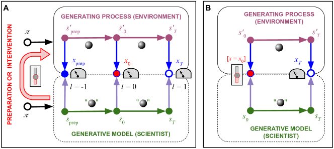
Figure 9: Active inference: (A) Graphical model characterizing active inference (cf. Figs. 1 and 2 in Ref. friston2017graphical as well as Figs. 2 and 3 in Ref. schwobel2018active ). The upper graphical model enclosed within a solid line is the generative process associated to the external system. The only accessible information about this generative process is the data it generates on the observer’s sensors. The lower graphical model enclosed within a dashed line is the generative model the observer has about the external world. (B) When the scientist performs the required actions to consistently transform the variable position $x_{\rm prep}$ into the same initial position $x_{0}$, she effectively removes all causal dependencies before the start of the experiment at time step $\ell=0$. This could be interpreted as a form of causal intervention on the system. We denote this here as $\textsc{do}[x=x_{0}]$.

Here we briefly discuss some aspects of active inference in the framework of a scientist carrying out an experiment. Although we present some technical details for the reader that may not be familiar with it, our main purpose is to highlight the main underlying concepts. In active inference the external world—an experimental system in this case—is considered as a generative process, while the organism—here a scientist—perceiving, interacting with, and learning about such an external world is considered as (or to have) a generative model (see Fig. 9; cf. Fig. 2 in Ref. friston2017graphical and Figs. 1 and 2 in Ref. schwobel2018active ). We discuss these in the next subsections, closely following Ref. schwobel2018active .

B.1.1 Experimental systems as generative processes

Following active inference, the scientist’s (controlled) environment, i.e. the experimental system, is considered hidden to her; she can only indirectly access it by the data it generates in her sensorium via her observations. In Fig. 9A we represent the environment by a Bayesian network enclosed within a solid rounded rectangle, which depends on the actions of the organism (external arrow pointing towards the solid rounded rectangle; cf. Fig. 2 in Ref. friston2017graphical ; see Sec. 2.1 in Ref. schwobel2018active ). Accordingly, the state of the environment at time step $\ell$ is described by hidden variables $s_{\ell}^{\prime}$ (top dark magenta circles) which can generate an observation $x_{\ell}$ (center blue and red circles) with a probability $\Omega_{\ell}(x_{\ell}|s_{\ell}^{\prime})$ (blue arrows pointing downwards).

The environment dynamics is specified by the transition probability $\Theta_{\ell}(s_{\ell+1}^{\prime}|s_{\ell}^{\prime},a_{\ell})$ that the environment is in state $s_{\ell+1}^{\prime}$ at time step $\ell+1$, given that at the previous time step its state was $s_{\ell}^{\prime}$ and the scientist performed action $a_{\ell}$, e.g., by moving some knobs. The dynamical dependency between hidden variables is represented in Fig. 9A by the top horizontal dark magenta arrows. The dependency of these dynamics on the scientist’s actions is represented by the black arrow external to the solid rounded rectangle and pointing towards it. This is to emphasize that the scientist can select a whole sequence of actions according to a behavioral policy schwobel2018active ; friston2017graphical , $\pi$, as discussed in the next subsection.

To keep the discussion at the minimal level of complexity required to illustrate the relevant concepts for our purpose, we focus here only on three time steps, $\ell=-1,0,1$ (see Fig. 9A). However, each transition from a time step $\ell$ to the next $\ell+1$ can be partitioned into as many time steps as desired schwobel2018active .

B.1.2 Scientists as generative models

Following active inference, the scientist is considered to be, or to have physically encoded in her neural system and perhaps body, a generative model of her (controlled) environment, i.e. of the experimental system. This generative model is represented in Fig. 9A by a Bayesian network within a dashed rounded rectangle, which mirrors the Bayesian network representing the environment. The generative model is defined as a joint probability distribution over observations $x_{\ell}$ (middle blue and red circles), internal “copies” $s_{\ell}$ of the environment’s hidden states $s_{\ell}^{\prime}$ (bottom green circles), which are encoded in the scientist’s neural system or body, and behavioral policies $\pi$ (black node external to the solid rounded square). The latter could be specified, for instance, by a sequence of control states $u_{\ell}$ (see Sec. 2.2 in Ref. schwobel2018active ), i.e. $\pi=(u_{-1},u_{0},u_{1})$, which denote a subjective abstraction of an action, such as a neuronal command to execute a specific action in the environment schwobel2018active . In Ref. schwobel2018active a one-to-one mapping is assumed between a selected control state $u_{\ell}$ and executed action $a_{\ell}$ in each time step $\ell$.

The generative model is represented in Fig. 9A by a Bayesian network within a dashed rounded rectangle, which mirrors the Bayesian network representing the environment. It can be written as schwobel2018active (see Eq. (2.4) therein)

$$\mathcal{P}^{\rm gen}(\mathbf{x},\mathbf{s},\pi)=p^{\rm pol}(\pi)p_{-1}(s_{-1})\prod_{\ell=0}^{1}\mathcal{P}^{\rm obs}_{\ell}(x_{\ell}|s_{\ell})\mathcal{P}_{\ell}^{\rm dyn}(s_{\ell}|s_{\ell-1},\pi),$$ (126)

where $\mathbf{x}=(x_{-1},x_{0},x_{1})$ and $\mathbf{s}=(s_{-1},s_{0},s_{1})$. Here $\mathcal{P}^{\rm dyn}$ (bottom horizontal green arrows in Fig. 9A) specifies the scientist’s model of the environment’s hidden dynamics, which can be affected by the actions the scientist performs according to the behavioral policy $\pi$. Furthermore, $\mathcal{P}_{\ell}^{\rm obs}$ (bottom purple arrows pointing upwards in Fig. 9A) specifies the model of how hidden states of the environment generate observations. Finally, $p_{-1}$ and $p^{\rm pol}$ are priors over the initial state of the environment and the policy, respectively.

Now, when carrying out an experiment a scientist first prepares the state of the experimental system at the start of the experiment, i.e., at time step $\ell=0$. Say the experimental system is a particle in a piece-wise linear potential (see Fig. 2A in the main text). This could be done, for instance, by performing a measurement at a previous time step, $\ell=-1$, say of the position of the particle $x_{-1}=x_{\rm prep}$ as displayed in a reading device—this would correspond to the first time step in Fig. 9A. Afterwards, the scientist can act on the system to consistently obtain a desired observation, $x_{0}=x_{0}^{\ast}$, at time step $\ell=0$ when the experiment starts.

For instance, the scientist can generate some commands that would lunch a mechanism that moves the particle an amount $x_{0}^{\ast}-x_{\rm prep}$ in such a way that the scientist consistently observes a given position, $x_{0}=x_{0}^{\ast}$, as displayed on a reading device, modulo experimental error. Different observations $x_{\rm prep}$ at time step $\ell=-1$ would lead to different actions. The aim of those actions is precisely that an observation at time step $\ell=0$ always yields the same result, $x_{0}=x_{0}^{\ast}$. Since the observation at time step $\ell=0$ yields consistently the same result, this effectively removes the dynamical dependencies before this time step, when the experiment starts. This amounts at a form of causal intervention. We denote this here as $\textsc{do}[x_{0}=x_{0}^{\ast}]$.

B.2 Enactivism: dynamical coupling between scientist and world

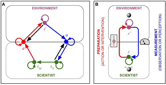
Figure 10: Enactivist framework: (A) Dependency graph of the enactive cognitive model described by Eqs. (127)-(131), as presented in Ref. di2017sensorimotor (see Ch. 3 and Fig. 3.5 therein; see also Ref. buhrmann2013dynamical ). Nodes represent variables. An arrow indicates that the variable it points to depends on the variable in its tail—in particular, circular arrows indicate recurrent dependencies. This dependency graph represents a circular interaction: scientist’s actions, $a$, influence the environment’s state, $s^{\prime}$; environment’s states influence the scientist’s sensor activity, $o$, via observations; sensor activity influences neural activity, $s_{N}$; neural activity influences motor activity, $s_{M}$, i.e. outflowing movement-producing signals; finally, motor activity influences scientist’s actions, which closes the interaction loop. Although, internal neural activity and environment’s states can influence back, respectively, sensor activity and scientist’s actions—e.g. by changing body configuration—the global dynamics is clockwise. (B) Simplified dependency graph that only shows the circular dependency between environment’s states, $s^{\prime}$, and scientist’s internal states, $s=(s_{M},s_{N})$. An action can prepare a desired state of the experimental system, e.g., a hand movement to turn a knob that places a particle in a desired location—in this sense it may be considered as a form of causal intervention. An observation can be mediated via a reading device, e.g. to determine the final position of the particle (see Fig. 2A in the main text).

Active inference, as briefly described above, still has a representationalist flavour in that the task of the scientist is to learn a model, i.e. a representation, as accurate as possible of the environment’s dynamics, including how her own actions affect it. The environment, which is described by the fixed probability distributions $\Theta_{\ell}$ and $\Omega_{\ell}$ in Sec. B.1.1, is considered as something externally given. This is reflected in that the topology of the Bayesian network representing the scientist mirrors the topology of the Bayesian network representing the environment. In particular, the internal and external dynamics (horizontal arrows in Fig. 9) flow in the same direction.

In contrast, the enactive approach varela2017embodied ; di2017sensorimotor ; gallagher2017enactivist puts a stronger emphasis on the dynamical coupling between scientist and environment buhrmann2013dynamical ; di2017sensorimotor . The focus is often on the particular sensor and motor systems of an individual like, e.g., a human or a robot. However, scientists manage to transcend their own sensorimotor limitations with the aid of technological devices that therefore enable them to couple to the world in “more fundamental” ways. For instance, the kind of manipulations and observations associated to light-matter interaction experiments are enabled by, e.g., lasers and electron microscopes. These kinds of couplings between scientists and world are hardly possible without such technologies. Such technologies are created by scientists themselves in their quest for lawful regularities. In this quest scientists have to learn how to build suitable experimental devices, how to stabilize the experimental system and achieve repeatability, how to obtain a decent measurement precision, etc. In general, how to achieve reliability—conditions R1-R3 in Sec. I in the main text. Our work is focused only on the post-learning stage, so it does not depend on a specific theory of learning.

From an enactive perspective, we could consider both the scientist and the environment as physical systems involved in a circular interaction possibly enabled by technological devices (see Fig. 10; cf. Fig. 3.5 in Ref. di2017sensorimotor ). However, to the best of our knowledge, the mathematical formalization of enactivism is not as well developed as that of active inference. Indeed, we are aware of only a couple of rather recent works buhrmann2013dynamical ; di2017sensorimotor that attempt to do that. Here we briefly discuss some of the main concepts underlying enactivism, closely following di2017sensorimotor (see Ch. 3 therein; see also Ref. buhrmann2013dynamical ).

For instance, the (controlled) environment or experimental system could be described by state variables $s^{\prime}$, e.g., the position of a particle in a piece-wise linear potential (see Fig. 2A in the main text). Similarly, we could use variables $a$ to represent actions the scientist perform on the experimental system, e.g. by moving her hand to turn a knob that puts the particle in a desired position—these kinds of actions could be considered effectively as state preparations or causal interventions. The dynamics of the environment can then be described by di2017sensorimotor

$$\frac{\mathrm{d}s^{\prime}}{\mathrm{d}t}=\mathcal{E}(s^{\prime},a),$$ (127)

where the function $\mathcal{E}$ captures the dependency of the environment’s current state on its previous state and the scientist’s previous actions.

The scientist’s sensor activity, here denoted by variables $o$, is influenced by the environment via her observations that stimulate her sensorium. Furthermore, in Refs. di2017sensorimotor ; buhrmann2013dynamical the scientist is assumed to have an internal neural dynamics, here described by variable $s_{N}$, which modulates the sensors activity. The scientist’s sensors’ dynamics can then be described by

$$\frac{\mathrm{d}o}{\mathrm{d}t}=\mathcal{O}(s^{\prime},s_{N}),$$ (128)

where the function $\mathcal{O}$ captures the dependency of the scientist’s sensor dynamics on the state of both the environment and the scientist’s internal neural dynamics.

The dynamics of neural activity is assumed to depend on sensor activity and on the neural activity itself, i.e.

$$\frac{\mathrm{d}s_{N}}{\mathrm{d}t}=\mathcal{N}(s,s_{N}),$$ (129)

where the function $\mathcal{N}$ captures such dependencies. Additionally, the scientist’s outflowing movement-producing signals, or motor activity, denoted here by $s_{M}$, is assumed to be influenced by the neural activity, $s_{N}$, i.e.

$$\frac{\mathrm{d}s_{M}}{\mathrm{d}t}=\mathcal{M}(s_{N}),$$ (130)

where the function $\mathcal{M}$ captures such an influence.

Finally, the interaction loop is closed by assuming the scientist’s actions, which can be implemented via body configurations, depend on the current actions she performs, on her internal motor activity, and on the state of the environment. So, the scientist’s actions dynamics can be described as

$$\frac{\mathrm{d}a}{\mathrm{d}t}=\mathcal{A}(a,s_{M},s^{\prime}),$$ (131)

where the function $\mathcal{A}$ captures such dependencies.

Appendix C Markov processes and imaginary-time quantum dynamics

Here we first discuss the principle of maximum dynamical entropy, or principle of maximum caliber. This is a general variational principle, similar to the free energy principle, from which a variety of models at, near, and far from equilibrium can be derived presse2013principles . We have used this principle in the main text to derive the form of the stationary distribution over the dynamical trajectories characterizing a scientist interacting with an experimental system. We here focus on chains for simplicity.

Afterwards, we show that the belief propagation (BP) algorithm, which is exact on chains, can be written in a way formally analogous to imaginary-time or Euclidean quantum dynamics Zambrini-1987 . More precisely, BP messages play the role of imaginary-time wave functions and the continuous-time limit of the BP iteration corresponds to the imaginary-time version of Schrödinger equation. However, in this case the BP messages on the leaves of the chain, which initiate the BP iteration, can always be chosen constant.

We then discuss the case of cycles which is more interesting. Indeed, the BP algorithm is not guaranteed to be exact anymore Weiss-2000 . However, we can choose initial and final conditions for the probability marginals to effectively turn the cycle into a chain. This yield the formal analogue of the general imaginary-time quantum dynamics considered in Ref. Zambrini-1987 .

C.1 Principle of maximum caliber and factor graphs

The principle of maximum entropy jaynes2003probability to derive some common equilibrium probability distributions in statistical physics can be extended to the so-called principle of maximum caliber to deal with non-equilibrium distributions on trajectories presse2013principles . In particular Markov chains and Markov processes can be derived from the principle of maximum caliber (see e.g. Sec. IX B in Ref. presse2013principles ). We introduce this principle here with an example relevant for our discussion.

Consider a probability distribution $\mathcal{P}_{\rm ch}(x_{1},\dotsc,x_{n})$ on (discretized) paths $(x_{1},\dotsc,x_{n})$, where $x_{\ell}$ refers to the position at time $t=\ell\epsilon$. Here we will consider the case of an open chain. Assume that we only have information about the average energy on the (discretized) paths given by

$$\mathcal{H}_{\rm av}[\mathcal{P}_{\rm ch}]=\left\langle\frac{1}{T}\sum_{\ell=0}^{n-1}\mathcal{H}_{\ell}(x_{\ell+1},x_{\ell})\epsilon\right\rangle_{\mathcal{P}_{\rm ch}},$$ (132)

where $T=n\epsilon$ is the total time duration of the path, and $\mathcal{H}_{\ell}$ is the “energy” or Hamiltonian-like function at time step $\ell$. Here

$$\left\langle f\right\rangle_{\mathcal{P}}=\int\mathcal{P}(x_{0},\dotsc,x_{n})f(x_{0},\dotsc,x_{n})\prod_{\ell=0}^{n-1}\mathrm{d}x_{\ell},$$ (133)

denotes the average value of a generic function $f$ of a path, with respect to a generic path probability distribution $\mathcal{P}$. For convenience, here we are using integrals instead of sums, as in the main text. However, our analysis is valid for discrete variables too by changing these integrals by sums, $\int\to\sum$.

The principle of maximum caliber tells us that among all possible probability distributions we should choose the one that both maximizes the entropy

$$\mathcal{S}[\mathcal{P}_{\rm ch}]=-\left\langle\ln\mathcal{P}_{\rm ch}(x_{0},\dotsc,x_{n})\right\rangle_{\mathcal{P}_{\rm ch}},$$ (134)

and is consistent with the information we have, i.e. $\mathcal{H}_{\rm av}[\mathcal{P}_{\rm ch}]=E_{\rm av}$, where $E_{\rm av}$ is the fixed value of the average energy. Introducing a Lagrange multiplier $\lambda$ to enforce the constraint on the average energy, the constrained maximization of $\mathcal{S}[\mathcal{P}_{\rm ch}]$ becomes equivalent to the maximization of the Lagrangian $\mathcal{S}[\mathcal{P}_{\rm ch}]-\lambda\mathcal{H}_{\rm av}[\mathcal{P}_{\rm ch}]$. The solution to this problem is the distribution

$$\mathcal{P}_{\rm ch}(x_{0},\dotsc,x_{n})=\frac{1}{\mathcal{Z}}\exp\left[-\frac{\lambda}{T}\sum_{\ell=0}^{n-1}\mathcal{H}_{\ell}(x_{\ell+1},x_{\ell})\epsilon\right],$$ (135)

where $\mathcal{Z}$ is the normalization factor.

Notice that $\mathcal{P}_{\rm ch}$ in Eq. (135) can be written as a product of factors

$$\mathcal{P}_{\rm ch}(x_{0},\dotsc,x_{n})=\frac{1}{Z}\prod_{\ell=0}^{n-1}F_{\ell}(x_{\ell+1},x_{\ell}).$$ (136)

Without loss of generality, we can choose the factors as

$$F_{\ell}(x_{\ell+1},x_{\ell})=\frac{1}{|\mathcal{A}|}\exp\left[-\frac{\lambda}{T}\mathcal{H}_{\ell}(x_{\ell+1},x_{\ell})\epsilon\right],$$ (137)

with $|\mathcal{A}|=\sqrt{2\pi T\epsilon/m\lambda}$, so $Z=\mathcal{Z}/|\mathcal{A}|^{n}$ in Eq. (136).

C.2 Quantum-like formulation of stochastic processes via the cavity method

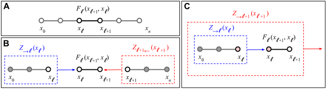
Figure 11: Cavity method. (A) Factor graph with the topology of a chain (see Eq. (136)). (B) Graphical expression for the pairwise marginal $\mathcal{P}_{\ell}(x_{\ell+1},x_{\ell})$ (see Eq. (138)); the partial partition functions $Z_{\to\ell}(x_{\ell})$ (blue; see Eq. (140)) and $Z_{\ell+1\leftarrow}(x_{\ell+1})$ (red; see Eq. (141)) correspond to the sum over all variables on the cavity graphs inside the dashed rectangles, except for $x_{\ell}$ and $x_{\ell+1}$ which are clamped to be able to recover the whole graphical model by multiplying for $F_{\ell}(x_{\ell+1},x_{\ell})$. (C) The partial partition function $Z_{\to\ell+1}(x_{\ell+1})$ (red) can be recursively computed by multiplying the partial function $Z_{\to\ell}(x_{\ell})$ and the factor $F_{\ell}(x_{\ell+1},x_{\ell})$ and tracing over $x_{\ell}$ (see Eq. (142)). This is the content of the belief propagation algorithm Mezard-book-2009 specified by Eqs. (142) and (143).

C.2.1 Cavity messages as imaginary-time wave functions

Here we show how the belief propagation algorithm obtained via the cavity method Mezard-book-2009 (ch. 14) can be formally written in terms of the imaginary-time Schrödinger equation and its conjugate. First, notice that by marginalizing the probability distribution defined in Eq. (136) over all variables except $x_{\ell}$ and $x_{\ell+1}$ we obtain

$$\mathcal{P}_{\ell}(x_{\ell+1},x_{\ell}) = \frac{1}{Z}F_{\ell}(x_{\ell+1},x_{\ell})Z_{\to\ell}(x_{\ell})Z_{\ell+1\leftarrow}(x_{\ell+1}),$$ (138)

$$p_{\ell}(x_{\ell}) = \sum_{x_{\ell+1}}\mathcal{P}_{\ell}(x_{\ell+1},x_{\ell})=\frac{1}{Z}Z_{\to\ell}(x_{\ell})Z_{\ell\leftarrow}(x_{\ell}),$$ (139)

where the partial partition functions $Z_{\to\ell}(x_{\ell})$ and $Z_{\ell\leftarrow}(x_{\ell})$ of the original factor graph are given by the partition functions of the modified factor graphs that contain all factors $F_{\ell^{\prime}}$ to the left (i.e. $\ell^{\prime}<\ell$) and to the right (i.e. $\ell^{\prime}\geq\ell$) of variable $x_{\ell}$, respectively; i.e. (see Fig. 11A,B; cf. Eq. (14.2) in Ref. Mezard-book-2009 ).

$$Z_{\to\ell}(x_{\ell}) = \int\prod_{\ell^{\prime}=0}^{\ell-1}F_{\ell^{\prime}}(x_{\ell^{\prime}+1},x_{\ell^{\prime}})\mathrm{d}x_{\ell^{\prime}},$$ (140)

$$Z_{\ell\leftarrow}(x_{\ell}) = \int\prod_{\ell^{\prime}=\ell}^{n-1}F_{\ell^{\prime}}(x_{\ell^{\prime}+1},x_{\ell^{\prime}})\mathrm{d}x_{\ell^{\prime}+1}.$$ (141)

$Z_{\to\ell}(x_{\ell})$ and $Z_{\ell\leftarrow}(x_{\ell})$ can be interpreted as information that arrives to variable $\ell$ from the left and from the right side of the graph, respectively.

By separating factor $F_{\ell-1}$ and $F_{\ell}$ in Eqs. (140) and (141), respectively, we can write these equations in a recursive way as (see Fig. 11C; cf. Eq. (14.5) in Ref. Mezard-book-2009 )

$$Z_{\to\ell}(x_{\ell}) = \int F_{\ell-1}(x_{\ell},x_{\ell-1})Z_{\to\ell-1}(x_{\ell-1})\mathrm{d}x_{\ell-1},$$ (142)

$$Z_{\ell\leftarrow}(x_{\ell}) = \int Z_{\ell+1\leftarrow}(x_{\ell+1})F_{\ell}(x_{\ell+1},x_{\ell})\mathrm{d}x_{\ell+1}.$$ (143)

These recursive equations are usually referred to as the belief propagation algorithm. Since the partial partition functions are typically exponentially large, Eqs. (142) and (143) are commonly written in terms of normalized cavity messages ${\nu_{\to\ell}(x)=Z_{\to\ell}(x)/Z_{\to\ell}}$ and ${\nu_{\ell\leftarrow}(x)=Z_{\ell\leftarrow}(x)/Z_{\ell\leftarrow}}$, where $Z_{\to\ell}$ and $Z_{\ell\leftarrow}$ are the corresponding normalization constants. This choice of normalization has at least two advantages: (i) it allows us to interpret the messages as probability distributions and (ii) it keeps the information traveling from left to right separated from the information traveling from right to left.

We will now show that a different choice of normalization, i.e.

$$\mu_{\to\ell}(x)=\frac{Z_{\to\ell}(x)}{\sqrt{Z}},\hskip 14.22636pt\mu_{\ell\leftarrow}(x)=\frac{Z_{\ell\leftarrow}(x)}{\sqrt{Z}},$$ (144)

which violates the features (i) and (ii) mentioned above, allows us to connect the BP equations, i.e. Eqs. (142) and (143), with those of Euclidean quantum mechanics. Indeed, let us write

$$\mu_{\to\ell}(x)\mu_{\ell\leftarrow}(x) = p_{\ell}(x),$$ (145)

$$\frac{\mu_{\to\ell}(x)}{\mu_{\ell\leftarrow}(x)} = e^{2\phi_{\ell}(x)},$$ (146)

where Eq. (145) comes from Eq. (139) and Eq. (146) is a definition of the “effective field” or “phase” $\phi_{\ell}$. Equations (145) and (146) imply that we can parametrize the cavity messages in terms of $p_{\ell}$ and $\phi_{\ell}$ as

$$\mu_{\to\ell}(x) = \sqrt{p_{\ell}(x)}e^{\phi_{\ell}(x)},$$ (147)

$$\mu_{\ell\leftarrow}(x) = \sqrt{p_{\ell}(x)}e^{-\phi_{\ell}(x)},$$ (148)

which are the analogue of a “wave function” in imaginary time.

C.2.2 Belief propagation as imaginary-time quantum dynamics

In terms of the messages $\mu_{\to\ell}$ and $\mu_{\ell\leftarrow}$ in Eq. (144), the belief propagation equations (142) and (143) become

$$\mu_{\to\ell}(x) = \int F_{\ell-1}(x,x^{\prime})\mu_{\to\ell-1}(x^{\prime})\mathrm{d}x^{\prime},$$ (149)

$$\mu_{\ell\leftarrow}(x) = \int\mu_{\ell+1\leftarrow}(x^{\prime})F_{\ell}(x^{\prime},x)\mathrm{d}x^{\prime},$$ (150)

where we have done $x_{\ell}=x$, $x_{\ell-1}=x^{\prime}$ in Eq. (149), and $x_{\ell+1}=x^{\prime}$ in Eq. (150). This contrasts with the standard formulation in terms of the $\nu$-messages described after Eq. (143), where the messages must be renormalized at each iteration of the belief propagation equations (cf. Eq. (14.2) in Ref. Mezard-book-2009 ). Such iterative renormalization is avoided here because the normalization constant $\sqrt{Z}$ is the same for all quantum-like cavity messages. Equations (149) and (150) are formally analogous to Eq. (2.16) in Ref. zambrini1986stochastic and its adjoint, respectively, which describe imaginary-time quantum dynamics.

For concreteness let us consider the energy function

$$\mathcal{H}_{\ell}(x,x^{\prime})=\frac{m}{2}\left(\frac{x-x^{\prime}}{\epsilon}\right)^{2}+V(x).$$ (151)

Due to the Gaussian term in the corresponding factors $F_{\ell}$ in Eq. (137), the integrals in Eqs. (149) and (150) can be approximated to first order in $\epsilon$. Indeed, since $\epsilon\to 0$, the real Gaussian factor associated to the quadratic term in Eq. (151) is exponentially small except in the region where ${|x-x^{\prime}|=O(\sqrt{\hbar\epsilon/m})}$. This allow us to estimate the integral to first order in $\epsilon$ by expanding the $\mu$ terms in Eqs. (149) and (150) around $x$ up to second order in ${x-x^{\prime}}$. Consistent with this approximation to first order in $\epsilon$, we can also do $\exp{[-V(x)\epsilon/\hbar]}=1-V(x)\epsilon/\hbar+O(\epsilon^{2})$ in factors $F_{\ell}$. In this way we get the equations

$$\mu_{\to\ell}(x) = \mu_{\ell-1}(x)-\frac{\lambda\epsilon}{T}V_{\ell}(x)\mu_{\to\ell}(x)+\frac{T\epsilon}{2m\lambda}\frac{\partial^{2}\mu_{\to\ell}(x)}{\partial x^{2}}+O(\epsilon^{2}),$$ (152)

$$\mu_{\ell\leftarrow}(x) = \mu_{\ell+1\leftarrow}(x)-\frac{\lambda\epsilon}{T}V_{\ell}(x)\mu_{\ell\leftarrow}(x)+\frac{T\epsilon}{2m\lambda}\frac{\partial^{2}\mu_{\ell\leftarrow}(x)}{\partial x^{2}}+O(\epsilon^{2}).$$ (153)

Now, to get the continuous-time limit, let ${\mu_{\to}(x,\ell\epsilon)=\mu_{\to\ell}(x)}$ and ${\mu_{\leftarrow}(x,\ell\epsilon)=\mu_{\ell\leftarrow}(x)}$, and expand ${\mu_{\to}(x,t-\epsilon)=\mu_{\to}(x,t)-\epsilon\dot{\mu}_{\to}}(x,t)$ as well as ${\mu_{\leftarrow}(x,t+\epsilon)=\mu_{\leftarrow}+\epsilon\dot{\mu}_{\leftarrow}(x,t)}$, where $t=\ell\epsilon$ and the dot operator stands for time derivative. So, taking $\epsilon\to 0$ we obtain

$$-\frac{T}{\lambda}\frac{\partial\mu_{\to}(x,t)}{\partial t} = -\frac{T^{2}}{2m\lambda^{2}}\frac{\partial^{2}\mu_{\to}(x,t)}{\partial x^{2}}+V(x,t)\mu_{\to}(x,t),$$ (154)

$$\frac{T}{\lambda}\frac{\partial\mu_{\leftarrow}(x,t)}{\partial t} = -\frac{T^{2}}{2m\lambda^{2}}\frac{\partial^{2}\mu_{\leftarrow}(x,t)}{\partial x^{2}}+V(x,t)\mu_{\leftarrow}(x,t),$$ (155)

which yields precisely the imaginary-time Schrödinger equation and its adjoint, with ${\Gamma}=T/\lambda$ playing the role of Planck constant $\hbar$. Indeed, Eqs. (154) and (155) are formally analogous to Eqs. (2.1) and (2.17) in Ref. Zambrini-1987 ; the analogous of $\theta$ and $\theta^{\ast}$ therein are here $\mu_{\leftarrow}$ and $\mu_{\to}$, respectively (but see Appendix C.3).

C.3 Euclidean quantum mechanics: From linear chains to cycles

Although Eqs. (154) and (155) look like imaginary-time quantum dynamics, things are not so interesting for chains. Indeed, the messages $\mu_{\to 0}$ and $\mu_{n\leftarrow}$, which correspond to the leaves of the chain and serve as the initial conditions for Eqs. (149) and (150), can always be chosen constant. The reason is that there are no factors before $F_{0}$ nor after $F_{n}$ The reason. In contrast, imaginary-time quantum dynamics involve more interesting initial and final conditions. Indeed, besides Eqs. (154) and (155), the imaginary-time quantum dynamics described in Ref. Zambrini-1987 is characterized by general initial and final conditions (see Eq. (2.14) therein).

We now show that, even though the BP algorithm is not exact on cycles Weiss-2000 , the dynamics can still be naturally formulated in terms of imaginary-time quantum dynamics. Assume that we know the initial and final single-variable marginals, $p_{0}$ and $p_{n}$. Conditioning on the initial and final variables turns the cycle into two chains (see Fig. 3 B): an “external” chain going from time step $0$ to time step $n$ (purple) and an “internal” chain going from time step $n$ to time step $k=2n$ (green). So, BP can become exact again on each chain, as long as the messages are consistent with the initial and final conditions. We will see that if the “external” dynamics are given by the probability matrix $P_{0}^{\rm ext}$ then the “internal” dynamics are given by the transposed matrix, i.e., $P_{\ell}^{\rm int}=\left[P_{\ell}^{\rm ext}\right]^{T}$. For generic initial and final conditions, we have that $P_{0}^{\rm ext}$ and $P_{n}^{\rm ext}$ are not necessarily symmetric and can be given by “pure states”, yet still satisfy an imaginary-time quantum dynamics. So, the results presented in the main text can in principle be extended to general probability matrices.

Indeed, we can formulate the dynamics on the “external” chain in terms of messages $\mu_{\to\ell}$ and $\mu_{\ell\leftarrow}$ satisfying Eqs. (149) and (150) as well as the initial and final conditions (cf. Eq. (2.14) in Ref. Zambrini-1987 )

$$p_{0}(x) = \mu_{\to 0}(x)\mu_{0\leftarrow}(x)$$ (156)

$$= \mu_{\to 0}(x)\int\mu_{n\leftarrow}(x^{\prime})\widetilde{F}_{0}(x^{\prime},x)\mathrm{d}x^{\prime},$$

$$p_{n}(x) = \mu_{\to n}(x)\mu_{n\leftarrow}(x)$$ (157)

$$= \left[\int\widetilde{F}_{0}(x,x^{\prime})\mu_{\to 0}(x^{\prime})\mathrm{d}x^{\prime}\right]\mu_{n\leftarrow}(x),$$

where $\widetilde{F}_{0}=F_{n-1}\cdots F_{0}$. In the continuous-time limit, this yields the formal analogue of the imaginary-time quantum dynamics presented in Ref. Zambrini-1987 .

We can also formulate the dynamics of the “internal” chain, which goes from time step $n$ to time step $k=2n$, in an analogous way. It is convenient to use $k-\ell$, with $\ell=0,\dots,n-1$, as time step index. The dynamics of the messages $\nu_{\to k-\ell}$ and $\nu_{k-\ell\leftarrow}$ for the “internal” chain satisfy

$$\nu_{\to k-\ell}(x) = \int{F}_{k-\ell-1}(x,x^{\prime})\nu_{\to k-\ell-1}(x^{\prime})\mathrm{d}x^{\prime},$$ (158)

$$\nu_{k-\ell\leftarrow}(x) = \int\nu_{k-\ell+1\leftarrow}(x^{\prime}){F}_{k-\ell}(x^{\prime},x)\mathrm{d}x^{\prime},$$ (159)

which are analogous to Eqs. (150) and (149). Furthermore, the $\nu$-messages must satisfy the boundary conditions

$$p_{n}(x) = \nu_{\to n}(x)\nu_{n\leftarrow}(x)$$ (160)

$$= \nu_{\to n}(x)\int\nu_{k\leftarrow}(x^{\prime})\widetilde{F}_{n}(x^{\prime},x)\mathrm{d}x^{\prime},$$

$$p_{k}(x) = \nu_{\to k}(x)\nu_{k\leftarrow}(x)$$ (161)

$$= \left[\int\widetilde{F}_{n}(x,x^{\prime})\nu_{\to n}(x^{\prime})\mathrm{d}x^{\prime}\right]\nu_{k\leftarrow}(x),$$

which are analogous to Eqs. (156) and (157). Here $\widetilde{F}_{n}=F_{k-1}\cdots F_{n}$ and $p_{k}=p_{0}$ as they refer to the same variable, $x_{0}$.

Now, taking into account that $F_{k-\ell-1}=F_{\ell}^{T}$ (see Eqs. (41) and (68) in the main text), Eqs. (158) and (159) become

$$\nu_{\to k-\ell}(x) = \int{F}_{\ell}^{T}(x,x^{\prime})\nu_{\to k-\ell-1}(x^{\prime})\mathrm{d}x^{\prime},$$

$$= \int\nu_{\to k-\ell-1}(x^{\prime}){F}_{\ell}(x^{\prime},x)\mathrm{d}x^{\prime}$$

$$\nu_{k-\ell\leftarrow}(x) = \int\nu_{k-\ell+1\leftarrow}(x^{\prime}){F}_{\ell-1}^{T}(x^{\prime},x)\mathrm{d}x^{\prime},$$

$$= \int{F}_{\ell-1}(x,x^{\prime})\nu_{k-\ell+1\leftarrow}(x^{\prime})\mathrm{d}x^{\prime}.$$

Equations (C.3) and (C.3) are equivalent to Eqs. (150) and (149), respectively. We can see this by doing (notice that arrows point in opposite directions)

$$\nu_{\to k-\ell} = \mu_{\ell\leftarrow},$$ (164)

$$\nu_{k-\ell\leftarrow} = \mu_{\to\ell}.$$ (165)

So, every solution to the “external” chain dynamics—characterized by a probability matrix $P^{\rm ext}_{\ell}(x,x^{\prime})=\mu_{\to\ell}(x)\mu_{\ell\leftarrow}(x^{\prime})$—yields, through Eqs. (164) and (165), a solution to the “internal” chain dynamics—characterized by a probability matrix $P^{\rm int}_{k-\ell}(x,x^{\prime})=\nu_{\to k-\ell}(x)\nu_{k-\ell\leftarrow}(x^{\prime})=P^{\rm ext}_{\ell}(x^{\prime},x)$. Using matrix notation, $P_{k_{\ell}}^{\rm int}=\left[P_{\ell}^{\rm ext}\right]^{T}$ is given by the transpose of $P_{\ell}^{\rm ext}$. In particular, $P_{k}^{\rm int}=\left[P_{0}^{\rm ext}\right]^{T}$ and $P_{n}^{\rm int}=\left[P_{n}^{\rm ext}\right]^{T}$. So, both solutions satisfy the corresponding boundary conditions since $p_{0}(x)=P^{\rm ext}_{0}(x,x)=P_{k}^{\rm int}(x,x)$ and $p_{n}(x)=P_{n}^{\rm ext}(x,x)=P_{n}^{\rm int}(x,x)$.

There are proofs of existence and uniqueness of the positive solutions of Eqs. (149) and (150) with the boundary conditions in Eqs. (156) and (157), for $p_{0}$ and $p_{n}$ without zeros, with various degrees of generality (see, e.g., Refs. zambrini1986stochastic ; Zambrini-1987 and references therein). Clearly, the same applies to Eqs (158) and (159) with the boundary conditions in Eqs. (160) and (161). In particular, they hold for the Hamiltonian in Eq. (13) in the main text.

Appendix D Hamiltonians with positive off-diagonal entries

Here we discuss the example of an infinite-dimensional quantum system described by factors with non-negative entries which, after truncation to its first two energy levels, turns into an effective system described by factors with negative off-diagonal entries. The latter is known as a two-level atom interacting with a coherent radiation field haken2005physics (see Sec. 15.3 therein).

Indeed, consider the Hamiltonian of an atom modeled as an electron, described by the momentum operator $i\hbar\nabla_{\mathbf{x}}$, moving in a potential field $V(\mathbf{x})$ produced by the nucleus,

$$H_{0}=-\frac{\hbar^{2}}{2m}\nabla_{\mathbf{x}}^{2}+V(\mathbf{x})=\sum_{n=0}^{\infty}E_{n}\left.|n\right\rangle\left\langle n\right|.$$ (166)

In the second equality we have expanded the Hamiltonian in terms of its eigenvalues $E_{n}$ and its eigenvectors $\left|n\right\rangle$, where $n$ is an integer, $n\geq 0$.

Now consider a perturbation

$$U(\mathbf{x},t)=e\mathbf{x}\cdot\mathbf{E}(t)=e\mathbf{x}\cdot\mathbf{E}_{0}\cos(\omega t),$$ (167)

so the perturbed Hamiltonian becomes ${H=H_{0}+U}$. Notice that the full Hamiltonian operator, $H$, can be derived via a path integral with Lagrangian

$$L=\frac{m}{2}\dot{\mathbf{x}}^{2}-V(\mathbf{x})-U(\mathbf{x},t).$$ (168)

We can also derive $H$ via a real non-negative factors or kernels (cf. Eq. (5))

$$\mathcal{K}_{\epsilon}(\mathbf{x}^{\prime},\mathbf{x})=e^{-\epsilon\mathcal{H}(\mathbf{x}^{\prime},\mathbf{x})/\hbar}\geq 0,$$ (169)

where

$$\mathcal{H}(\mathbf{x}^{\prime},\mathbf{x})=\frac{m}{2}\left(\frac{\mathbf{x}^{\prime}-\mathbf{x}}{\epsilon}\right)^{2}+V\left(\frac{|\mathbf{x}^{\prime}+\mathbf{x}|}{2}\right)+U(t).$$ (170)

We will now see that, after a standard truncation of the full Hamiltonian $H=H_{0}+U$ (see Eqs. (166) and (167)) into an effective two-level system, we lose the equivalence with the positive kernel given by Eqs. (169) and (170). Indeed, in the derivation of the Hamiltonian of a two-level atom it is usually assumed that the perturbation defined in Eq. (167) is near resonance with two relevant energy levels of the Hamiltonian $H_{0}$, say $E_{0}$ and $E_{1}$, i.e. $|\omega-\omega_{0}|\lll\omega_{0}$, where ${\hbar\omega_{0}=E_{1}-E_{0}}$. In this case, it is usually assumed that only the dynamics of these two energy levels matter. So, we can write

$$\begin{split}H=&E_{0}\left|0\right\rangle\left\langle 0\right|+E_{1}\left|1\right\rangle\left\langle 1\right|+U_{01}\left(\left|0\right\rangle\left\langle 1\right|+\left|1\right\rangle\left\langle 0\right|\right)\\ &+H_{\mathcal{R}},\end{split}$$ (171)

where the first three terms in the right hand side of Eq. (171) correspond to the transitions taking place within the subspace spanned by $\{\left|0\right\rangle,\left|1\right\rangle\}$, and

$$\begin{split}H_{\mathcal{R}}=&\sum_{n=2}^{\infty}E_{n}\left.|n\right\rangle\left\langle n\right|\\ &+\sum_{m=0}^{\infty}\sum_{n>m,n\neq 0,1}^{\infty}\left(U_{mn}\left|m\right\rangle\left\langle n\right|+U_{nm}\left|n\right\rangle\left\langle m\right|\right),\end{split}$$ (172)

collects all the remaining transitions. Here we have written

$$U_{mn}=U_{nm}^{\ast}=\left\langle m\right|U(t)\left|n\right\rangle,$$ (173)

for $m,n$ integers, $m,n\geq 0$. For the sake of illustration, we are restricting here to the case where $U_{01}=U^{\ast}_{01}$ can be chosen to be real and $U_{00}=U_{11}=0$ haken2005physics (see Sec. 15.3 therein); this explains the form of Eq. (171).

At this point it is argued that we can neglect $H_{\mathcal{R}}$ since the system is near resonance. This yields the effective two-level Hamiltonian

$$H_{\rm eff}=\overline{E}{\rm 1\!\!I}^{(01)}-\frac{\hbar\omega_{0}}{2}\sigma_{Z}^{(01)}+D\cos(\omega t)\sigma_{X}^{01},$$ (174)

where $\overline{E}=(E_{0}+E_{1})/2$, $D=\left\langle 0\right|\mathbf{r}\cdot\mathbf{E}_{0}\left|1\right\rangle$, and

$${\rm 1\!\!I}^{(01)} = \left|0\right\rangle\left\langle 0\right|+\left|1\right\rangle\left\langle 1\right|,$$ (175)

$$\sigma_{X}^{(01)} = \left|0\right\rangle\left\langle 1\right|+\left|1\right\rangle\left\langle 0\right|,$$ (176)

$$\sigma_{Z}^{(01)} = \left|0\right\rangle\left\langle 0\right|-\left|1\right\rangle\left\langle 1\right|.$$ (177)

If we now try to write this as a real factor

$$F_{\rm eff}={\rm 1\!\!I}+\epsilon J_{\rm eff},$$ (178)

with $J_{\rm eff}=-H_{\rm eff}/\hbar$, we end up with off-diagonal negative entries due to the factor $\cos(\omega t)$ accompanying $\sigma_{X}$ in Eq. (174). So, the full Hamiltonian $H=H_{0}+U$ in Eq. (171) can be represented in terms of the real positive kernel given by Eqs. (169) and (170), but the truncated effective Hamiltonian $H_{\rm eff}$ in Eq. (174) cannot. What happened? The full factor $F={\rm 1\!\!I}-\epsilon H/\hbar$ associated to kernel $\mathcal{K}_{\epsilon}$ (see Eqs. (169) and (171)), which has only non-negative entries, can be written as

$$F=\mathcal{R}+F_{\rm eff}.$$ (179)

So, even though the effective factor $F_{\rm eff}$ in Eq. (178) can have negative off-diagonal entries, those would be “corrected” by the “reference” term $\mathcal{R}=-\epsilon H_{\mathcal{R}}/\hbar$ yielding only positive quantities with a clear probabilistic interpretation.

References

- (1) F. J. Varela, E. Thompson, and E. Rosch, The embodied mind: Cognitive science and human experience (revised edition). MIT press, 2017.
- (2) E. Thompson, Mind in life. Harvard University Press, 2010.
- (3) E. Di Paolo, T. Buhrmann, and X. Barandiaran, Sensorimotor life: An enactive proposal. Oxford University Press, 2017.
- (4) L. Shapiro, Embodied cognition. Routledge, 2019.
- (5) Z. Djebbara, L. B. Fich, L. Petrini, and K. Gramann, “Sensorimotor brain dynamics reflect architectural affordances,” Proceedings of the National Academy of Sciences, vol. 116, no. 29, pp. 14769–14778, 2019.
- (6) M. Wilson, “Six views of embodied cognition,” Psychonomic bulletin & review, vol. 9, no. 4, pp. 625–636, 2002.
- (7) B. Bridgeman and P. Tseng, “Embodied cognition and the perception–action link,” Physics of life reviews, vol. 8, no. 1, pp. 73–85, 2011.
- (8) K. Friston, “Life as we know it,” Journal of the Royal Society Interface, vol. 10, no. 86, p. 20130475, 2013.
- (9) M. Velmans, Understanding consciousness. Routledge, 2009.
- (10) E. Thompson, Waking, dreaming, being: Self and consciousness in neuroscience, meditation, and philosophy. Columbia University Press, 2014.
- (11) M. Bitbol, “Is consciousness primary?,” NeuroQuantology, vol. 6, pp. 53–71, 2008.
- (12) C. Rovelli, “Relational quantum mechanics,” International Journal of Theoretical Physics, vol. 35, p. 1637, 1996.
- (13) G. M. D’Ariano, G. Chiribella, and P. Perinotti, Quantum theory from first principles: An informational approach. Cambridge University Press, 2017.
- (14) K. Friston, “The free-energy principle: a unified brain theory?,” Nature Reviews Neuroscience, vol. 11, no. 2, pp. 127–138, 2010.
- (15) S. Schwöbel, S. Kiebel, and D. Marković, “Active inference, belief propagation, and the bethe approximation,” Neural Computation, vol. 30, no. 9, pp. 2530–2567, 2018.
- (16) S. Pressé, K. Ghosh, J. Lee, and K. A. Dill, “Principles of maximum entropy and maximum caliber in statistical physics,” Reviews of Modern Physics, vol. 85, no. 3, p. 1115, 2013.
- (17) J. Pearl, Causality. Cambridge university press, 2009.
- (18) J. C. Zambrini, “Euclidean quantum mechanics,” Physical Review A, vol. 35, pp. 3631–3649, May 1987.
- (19) Y. Weiss, “Correctness of local probability propagation in graphical models with loops,” Neural Computation, vol. 12, pp. 1–41, 2000.
- (20) M. Mezard and A. Montanari, Information, Physics, and Computation. Oxford Graduate Texts, Oxford University Press, USA, 2009.
- (21) J. Zambrini, “Stochastic mechanics according to E. Schrödinger,” Physical Review A, vol. 33, no. 3, p. 1532, 1986.
- (22) J. B. DeBrota and B. C. Stacey, “FAQBism,” arXiv preprint arXiv:1810.13401, 2018.
- (23) N. D. Mermin, “Making better sense of quantum mechanics,” Reports on Progress in Physics, vol. 82, no. 1, p. 012002, 2018.
- (24) C. A. Fuchs, N. D. Mermin, and R. Schack, “An introduction to qbism with an application to the locality of quantum mechanics,” American Journal of Physics, vol. 82, no. 8, pp. 749–754, 2014.
- (25) J. P. Crutchfield, “Space-time dynamics in video feedback,” Physica D: Nonlinear Phenomena, vol. 10, no. 1-2, pp. 229–245, 1984.
- (26) C. Rovelli, Quantum gravity. Cambridge university press, 2007.
- (27) T. W. Deacon, Incomplete nature: How mind emerged from matter. WW Norton & Company, 2011.
- (28) S. Dehaene, H. Lau, and S. Kouider, “What is consciousness, and could machines have it?,” Science, vol. 358, no. 6362, pp. 486–492, 2017.
- (29) H. Haken and H. C. Wolf, The physics of atoms and quanta: introduction to experiments and theory, vol. 1439. Springer Science & Business Media, 2005.
- (30) W. Vinci and D. A. Lidar, “Non-stoquastic hamiltonians in quantum annealing via geometric phases,” npj Quantum Information, vol. 3, no. 1, p. 38, 2017.
- (31) H. Padmanabhan and T. Padmanabhan, “Nonrelativistic limit of quantum field theory in inertial and noninertial frames and the principle of equivalence,” Physical Review D, vol. 84, no. 8, p. 085018, 2011.
- (32) R. Feynman, A. Hibbs, and D. Styer, Quantum mechanics and path integrals—Emended edition. Dover Books on Physics, Dover Publications, 2010.
- (33) Y. Aharonov and D. Rohrlich, Quantum paradoxes: quantum theory for the perplexed. John Wiley & Sons, 2008.
- (34) Č. Brukner, “Facts are relative,” Nature Physics, vol. 16, no. 12, pp. 1172–1174, 2020.
- (35) N. D. Mermin, “Physics: Qbism puts the scientist back into science,” Nature, vol. 507, no. 7493, pp. 421–423, 2014.
- (36) C. A. Fuchs and R. Schack, “Quantum-bayesian coherence,” Reviews of Modern Physics, vol. 85, no. 4, p. 1693, 2013.
- (37) J. Pienaar, “Qbism and relational quantum mechanics compared,” Foundations of Physics, vol. 51, no. 5, pp. 1–18, 2021.
- (38) Č. Brukner, “On the quantum measurement problem,” in Quantum [Un] Speakables II, pp. 95–117, Springer, 2017.
- (39) C. Rovelli, Helgoland: Making Sense of the Quantum Revolution. Penguin, 2021.
- (40) D. R. Hofstadter, I am a strange loop. Basic books, 2013.
- (41) Y.-Y. Tang, B. K. Hölzel, and M. I. Posner, “The neuroscience of mindfulness meditation,” Nature Reviews Neuroscience, vol. 16, no. 4, pp. 213–225, 2015.
- (42) K. J. Friston, T. Parr, and B. de Vries, “The graphical brain: belief propagation and active inference,” Network Neuroscience, vol. 1, no. 4, pp. 381–414, 2017.
- (43) T. Buhrmann, E. A. Di Paolo, and X. Barandiaran, “A dynamical systems account of sensorimotor contingencies,” Frontiers in Psychology, vol. 4, p. 285, 2013.
- (44) S. Gallagher, Enactivist interventions: Rethinking the mind. Oxford University Press, 2017.
- (45) E. T. Jaynes, Probability theory: the logic of science. Cambridge University Press, 2003.