Channel Estimation for Hybrid Massive MIMO Systems with Adaptive-Resolution ADCs

Abstract

Achieving high channel estimation accuracy and reducing hardware cost as well as power dissipation constitute substantial challenges in the design of massive multiple-input multiple-output (MIMO) systems. To resolve these difficulties, sophisticated pilot designs have been conceived for the family of energy-efficient hybrid analog-digital (HAD) beamforming architecture relying on adaptive-resolution analog-to-digital converters (RADCs). In this paper, we jointly optimize the pilot sequences, the number of RADC quantization bits and the hybrid receiver combiner in the uplink of multiuser massive MIMO systems. We solve the associated mean square error (MSE) minimization problem of channel estimation in the context of correlated Rayleigh fading channels subject to practical constraints. The associated mixed-integer problem is quite challenging due to the nonconvex nature of the objective function and of the constraints. By relying on advanced fractional programming (FP) techniques, we first recast the original problem into a more tractable yet equivalent form, which allows the decoupling of the fractional objective function. We then conceive a pair of novel algorithms for solving the resultant problems for codebook-based and codebook-free pilot schemes, respectively. To reduce the design complexity, we also propose a simplified algorithm for the codebook-based pilot scheme. Our simulation results confirm the superiority of the proposed algorithms over the relevant state-of-the-art benchmark schemes.

I Introduction

Massive multiple-input multiple-output (MIMO) systems rely on a large number of base station (BS) antennas for simultaneously serving a few dozens of users, while striking an attractive spectral efficiency (SE) vs. energy efficiency (EE) trade-off [1, 2, 3]. However, a large number of antennas inevitably lead to an excessive radio-frequency (RF) hardware cost and energy consumption. Hence, a hardware-efficient hybrid analog-digital (HAD) beamforming architecture has been proposed as an alternative to the fully digital beamformer for practical implementation. Explicitly, this architecture relies on an analog beamformer in the RF domain combined with a low-dimensional digital beamformer in the baseband, hence allowing a significant reduction in the number of RF chains required. This in turn provides increased design flexibility for striking an attractive performance vs. complexity trade-off. The receiver’s power dissipation is dominated by that of the analog-to-digital converters (ADCs), since it increases exponentially with the number of quantization bits [4],[5]. Hence, low-resolution ADCs (LADCs) have been advocated for the RF chains of HAD receivers.

I-A Related Work

Extensive research efforts have been invested in the design and performance evaluation of hybrid beamformers [7, 8, 9, 10, 11, 12, 13, 14]. Basically, the existing hybrid beamforming architectures can be mainly divided into the static partially-connected structure [8, 9, 10], the static fully-connected structure [8, 9, 11], and the dynamic partially-connected or fully-connected structure [12, 13, 14]. The authors of [8] considered a single-user millimeter wave (mmWave) MIMO system and treated the hybrid beamforming weight design as a matrix factorization problem. Efficient alternating optimization algorithms were developed for both static partially-connected and static fully-connected structures. As a further exploration, the authors of [9] proposed heuristic algorithms for the design of static partially-connected and fully-connected HAD beamformers, permitting to maximize the overall SE of a broadband orthogonal frequency-division multiplexing (OFDM)-based system. Besides, the proposed algorithm in [9] for the fully-connected structure can achieve SE close to that of the optimal fully-digital solution with much less number of RF chains. Moreover, to dynamically adapt to the spatial channel covariance matrix and improve the system performance, [12, 13, 14] proposed to design the dynamic-connected HAD beamforming architecture to realize a flexible analog beamforming matrix. In [12], a dynamic sub-array approach was considered for OFDM systems, and a greedy algorithm to optimize the array partition based on the long-term channel characteristics was suggested. Different from the partially-adaptive-connected structure in [12], the authors in [13] proposed to implement the hybrid precoder with a fully-adaptive-connected structure. A joint optimization of switch-controlled connections and the hybrid precoders was formulated as a large-scale mixed-integer nonconvex problem with high dimensional power constraints. By modifying the on-off states of switch-controlled connections, this fully-adaptive-connected structure can realize a fully-connected structure or any possible sub-connected structure. Furthermore, the HAD beamforming strategy has also been investigated in the context of novel relay-aided systems [15, 16] and in Terahertz communications [17]. Since employing LADCs in the massive MIMO regime has become indispensable for reducing the power consumption and hardware cost, it has catalyzed substantial interest in the recent literature. The authors of [18] analyzed the performance for transmission over flat-fading MIMO channel using single-bit ADC and derived the capacity upper-bound both at infinite and finite signal-to-noise ratios (SNR). The impact of the spatial correlation of antennas on the rate loss caused by the coarse quantization of LADCs was further studied in [19], where the authors concluded that LADCs can achieve a sum rate performance much closer to the case of ideal ADCs under spatially correlated channels.

On account of the benefits provided by HAD beamformers and LADCs, a number of studies have been proposed to characterize the performance of massive MIMO systems relying on the HAD beamforming architecture using LADCs. The pioneering contribution of [20] proposed a generalized hybrid architecture using LADCs and verified that the achievable rate is comparable to that obtained by high-precision ADC based receivers at low and medium SNRs, which provides valuable insights for future research. Intensive research efforts have also been dedicated to analog/digital beamforming design [21, 22], to SE/EE optimization [23, 24, 25], to channel estimation [26] and to signal detection [27].

However, previous research on HAD beamforming using LADCs has mainly considered uniform quantizers having a fixed, predetermined number of bits, which limited the performance of these systems due to coarse quantization. As a further advance, it was shown that a variable-resolution ADC or adaptive-resolution ADC (RADC) architecture is preferable [28, 29]. In [28], the authors investigated a mixed-ADC structure designed for cloud radio access networks (C-RAN). In particular, they developed an ADC-resolution selection algorithm for maximizing either the SE or EE based on an approximation of the generalized mutual information in the low-SNR regime. In [29], the authors developed a pair of ADC bit allocation strategies for minimizing the quantization error effects under a total ADC power constraint, thereby achieving an improved performance. However, the separate design of the ADC quantization bit allocation and hybrid beamforming matrices tends to suffer from performance degradation. Hence, the authors of [30] jointly optimized both the on/off modes of the RF processing chains and the number of ADC quantization bits.

As a further development, the authors of [31] aimed for jointly optimizing the sampling resolution of ADCs and the hybrid beamforming matrices, which results in energy efficient solutions for point-to-point mmWave MIMO systems. In light of [31], the authors of [32] extended the joint design to multiuser systems, hence achieving a significantly improved EE compared to the existing schemes. The potential advantages of RADCs in the context of various practical systems have also been reported in [33, 34, 35]. The authors of [33] focused their attention on the uplink of mmWave systems using RADCs and investigated the associated joint resource allocation and user scheduling problem. In [35] the design of the reconfigurable intelligent surface (RIS) aided mmWave uplink system relying on RADCs was investigated, demonstrating that an RIS is capable of mitigating the performance erosion imposed by RADCs.

Nevertheless, the aforementioned studies are mainly based on perfect instantaneous channel state information (CSI), which is assumed to be known at the BS. In practice, the acquisition of perfect CSI cannot be achieved in massive MIMO systems due to the inevitable channel estimation errors [36]. Therefore, how to efficiently design the pilot signals for improving the precision of channel estimation is of paramount importance. In practice a codebook-based pilot scheme is preferred, where orthogonal pilot sequences are chosen from a given codebook as a benefit of its low-complexity implementation and low feedback overhead [37, 38]. However, allocating mutually orthogonal pilot sequences to a large number of users for avoiding interference during channel estimation would require excessive pilot lengths and their orthogonality would still be destroyed upon convolution with the dispersive channel impulse response (CIR). For this reason, the carefully constructed reuse of a limited set of orthogonal pilot sequences for different users for example is of paramount importance for high-precision channel estimation. Further design alternatives were proposed for massive MIMO systems for example in [38, 39], which dispense with a codebook, hence they may be termed as codebook-free solutions. However, they tend to require a higher feedback overhead for attaining a high channel estimation accuracy.

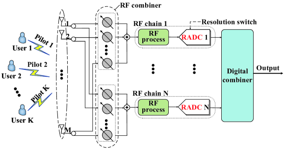
Figure 1: A multiuser massive MIMO uplink system adopting hybrid combiners with adaptive-resolution ADCs.

I-B Main Contributions

Despite the above advances, there is a paucity of research contributions on jointly optimizing the pilot sequences, the number of ADC quantization bits, and the HAD combiner for achieving high-precision channel estimation in the uplink of a multiuser massive MIMO system employing RADCs. Hence our inspiration is to fill this knowledge-gap. In particular, both codebook-based and codebook-free pilot schemes are investigated, where for each scheme, we aim to minimize the mean square error (MSE) of the channel estimate subject to a transmit power constraint, to the constant-modulus constraint imposed on the elements of the analog combining matrix, and to the additional constraints on the number of quantization bits. In a nutshell, the main contributions of this paper over the existing literature lie in the following:

• We focus on jointly optimizing the pilot sequences, the HAD combiners and the RADC bit allocation in the presence of a correlated Rayleigh fading channel model. The channel estimation mean square error (MSE) minimization problem is formulated, which only requires the knowledge of channel statistics under practical operating conditions.

• We first transform the highly nonconvex optimization problem into an equivalent but more tractable form by introducing auxiliary variables and employing fractional programming (FP) techniques. Then, we develop a new block coordinate descent (BCD) based algorithm for a codebook-free channel estimation scheme and a penalty dual decomposition (PDD) based algorithm for a codebook-based channel estimation scheme. Both of these iterative algorithms ensure convergence to the set of stationary solutions of the original optimization problem. Furthermore, the computational complexity of the proposed algorithms is analyzed.

• A simplified low-complexity algorithm is also presented for the codebook-based channel estimation scheme, which solves the MSE minimization problem suboptimally but efficiently.

• To characterize the benefits of our proposed algorithms, we provide exhaustive simulation results in terms of the MSE, sum rate and feedback overhead for a range of pertinent system settings. We demonstrate that through the coordinated allocation of bits to the RADCs, the proposed algorithms can beneficially exploit the knowledge of channel statistics to accomplish the pilot design, while minimizing interference and improving the channel estimation accuracy.

I-C Organization and Notation

This paper is organized as follows. In Section II and III, we introduce the investigated system model and formulate the optimization problem for the constrained channel estimation, respectively. In Section IV and V, we propose efficient algorithms by solving the formulated problems for the codebook-free and codebook-based pilot schemes, respectively. Section VI provides simulation results to appraise the performance of the proposed algorithms. The paper is concluded in Section VII, whilst proofs and detailed derivations appear in the Appendices.

Notations: For a matrix $\mathbf{M}$, $(\mathbf{M})^{T}$, $(\mathbf{M})^{*}$, $(\mathbf{M})^{H}$, and $\mathrm{vec}(\mathbf{M})$ denote its transpose, conjugate, conjugate transpose and vectorization, respectively. $\mathbf{M}(i,j)$ denotes the element at the intersection of row $i$ and column $j$. For a square matrix $\mathbf{M}$, $\mathrm{Tr}(\mathbf{M})$, $\mathbf{M}^{-1}$, and $\|\mathbf{M}\|_{F}$ represents its trace, inverse and Frobenius norm, respectively. $\mathrm{diag}(\mathbf{M})$ denotes a diagonal matrix consisting of the diagonal elements of $\mathbf{M}$. $\mathbf{I}$ denotes an identity matrix. For a vector $\mathbf{m}$, $\mathrm{diag}(\mathbf{m})$ denotes a diagonal matrix with $\mathbf{m}$ along its main diagonal and $\|\mathbf{m}\|$ denotes the Euclidean norm of vector $\mathbf{m}$. The symbol $\otimes$ denotes the Kronecker product. $\Re\{\cdot\}$ and $|\cdot|$ respectively denote the real and magnitude parts of a complex number. $\lfloor x\rfloor$ denotes the largest integer less than or equal to $x$ and $\lceil x\rceil$ denotes the smallest integer greater than or equal to $x$. We let $\mathbb{C}^{m\times n}$ ($\mathbb{R}^{m\times n}$) denote $m\times n$ complex (real) space. $\mathbb{E}[\cdot]$ denotes the expectation and $\mathcal{CN}(0,\sigma^{2})$ denotes the circularly symmetric complex Gaussian distribution with mean 0 and variance $\sigma^{2}$.

II System Model

As shown in Fig. 1, we consider a multiuser massive MIMO uplink system that adopts a static fully-connected hybrid AD combining structure with RADCs at the BS. The BS which is equipped with $M>1$ antennas and $N\ll M$ RF chains, serves $K$ single-antenna users simultaneously. The baseband output of each RF chain is fed to a dedicated RADC that employs variable bit resolution to quantize the real and imaginary parts of each analog signal. Moreover, we assume that the BS and users are fully time-synchronized.

II-A Channel Model

Without loss of generality, we consider a narrowband correlated channel model. Let $\mathbf{h}_{k}\in\mathbb{C}^{M\times 1}$ represent the uplink channel from user $k\in\mathcal{K}\triangleq\{1,\ldots,K\}$ to the BS. Then, the channel vector $\mathbf{h}_{k}$ can be expressed as

$$\mathbf{h}_{k}=\mathbf{R}_{k}^{\frac{1}{2}}\mathbf{g}_{k},$$ (1)

where $\mathbf{g}_{k}\in\mathbb{C}^{M\times 1}$ is a vector with independent and identically distributed (i.i.d.) elements distributed as $\mathcal{CN}(0,1)$, and $\mathbf{R}_{k}=\mathbb{E}[\mathbf{h}_{k}\mathbf{h}_{k}^{H}]$ denotes the channel covariance matrix for user $k$. $\mathbf{R}_{k}$ describes the spatial correlation properties of the channel due to macroscopic effects of propagation, including path-loss and shadowing. When the users are quasi-stationary, the path-loss and shadowing can be readily obtained based on the distance between the BS and user $k$ and stored at the BS as a priori [40],[41].

$$\mathrm{vec}(\mathbf{y}_{k})= (\mathbf{s}_{k}\otimes\mathbf{v}_{k}\mathbf{Q}_{\alpha}\mathbf{U})\mathbf{h}_{k}+\sum_{i\neq k}^{K}(\mathbf{s}_{i}\otimes\mathbf{v}_{k}\mathbf{Q}_{\alpha}\mathbf{U})\mathbf{h}_{i}\!+\!(\mathbf{I}_{\tau}\otimes\mathbf{v}_{k}\mathbf{Q}_{\alpha}\mathbf{U})\mathrm{vec}(\mathbf{Z})\!+\!(\mathbf{I}_{\tau}\otimes\mathbf{v}_{k})\mathrm{vec}(\mathbf{Z}_{q}).$$ (9)

II-B Pilot Sequences

In this work, we focus on two types of pilot sequences, i.e., the codebook-free and codebook-based pilots. For ease of exposition, we denote as $\mathbf{s}_{k}\in\mathbb{C}^{\tau\times 1}$ as the pilot sequence transmitted by user $k\in\mathcal{K}$, where $\tau<K$ is the length of the pilot sequence during each coherence interval. It is noteworthy that $\tau$ is predetermined based on the coherence budget.

1) Codebook-free pilots: As in previous works [38],[42], we assume that each pilot sequence $\mathbf{s}_{k}$ can be arbitrarily selected from the $\tau$-dimensional space under the power constraint:

$$\mathbf{s}_{k}\in\mathbb{C}^{\tau\times 1}\quad\text{with}\quad\|\mathbf{s}_{k}\|^{2}\leq P_{k}^{\textrm{max}},$$ (2)

where $P_{k}^{\textrm{max}}$ denotes the transmit power budget for user $k$.

2) Codebook-based pilots: We denote the available codebook as $\Upsilon=\{\bm{\upsilon}_{1},\bm{\upsilon}_{2},\cdots,\bm{\upsilon}_{\tau}\}$, where $\bm{\upsilon}_{\iota}\in\mathbb{C}^{\tau\times 1}$ denotes the $\iota$-th ($\iota\in\mathcal{T}\triangleq\{1,\ldots,\tau\}$) potential pilot sequence. It is assumed that the different pilot sequences meet the orthonormality conditions, i.e., $\bm{\upsilon}_{\iota}^{H}\bm{\upsilon}_{\iota^{\prime}}=0$, $\forall\iota\neq\iota^{\prime}$ and $\|\bm{\upsilon}_{\iota}\|^{2}=1,\forall\iota$. Then, the pilot sequence of user $k$ is constructed as

$$\mathbf{s}_{k}=\sqrt{p_{k}}\bm{\varrho}_{k}\quad\text{with}\quad\|\mathbf{s}_{k}\|^{2}\leq P_{k}^{\textrm{max}},$$ (3)

where $p_{k}$ denotes the transmit power of user $k$ and $\bm{\varrho}_{k}\in\Upsilon$ denotes the codebook sequence allocated to user $k$.

II-C Uplink Training

In the uplink training phase, the BS estimates the uplink channels based on the pilot sequences simultaneously transmitted from the users. Focusing on the $k$-th user, the received pilot signal at the BS can be expressed as

$$\mathbf{Y}=\mathbf{h}_{k}\mathbf{s}_{k}^{T}+\sum_{i\neq k}^{K}\mathbf{h}_{i}\mathbf{s}_{i}^{T}+\mathbf{Z},$$ (4)

where the first term represents the desired contribution from user $k$, the second term represents multiuser interference, and $\mathbf{Z}\in\mathbb{C}^{M\times\tau}$ denotes the additive complex Gaussian noise matrix with i.i.d. entries following the distribution $\mathcal{CN}(0,\sigma^{2})$.

An analog combining matrix $\mathbf{U}\in\mathbb{C}^{N\times M}$ is employed to process the received signal $\mathbf{Y}$ at the BS with the goal of suppressing interference from the other users. In the HAD architecture, the analog combiner is typically implemented using phase shifters [9], which imposes constant-modulus constraints on the elements of the matrix $\mathbf{U}$. The output of the analog combiner is given by

$$\bar{\mathbf{Y}}=\mathbf{U}(\mathbf{h}_{k}\mathbf{s}_{k}^{T}+\sum_{i\neq k}^{K}\mathbf{h}_{i}\mathbf{s}_{i}^{T}+\mathbf{Z}).$$ (5)

We employ RADCs to quantize $\bar{\mathbf{Y}}$ as shown in Fig. 1, which enables flexible quantization bit allocation for each baseband channel according to the radio propagation characteristics. Such a refined design can efficiently mitigate the quantization errors and greatly improve the system performance with reduced hardware cost and power consumption. Let integer $b_{n}$ denote the number of available quantization bits of RADC $n$. Assuming that the gain of automatic gain control is appropriately set, the additive quantization noise model (AQNM) can be employed to reformulate the quantized signal [29]. Then, based on the AQNM, the quantized output is specialized to

$$\mathbf{Y}_{q}=\mathcal{F}(\bar{\mathbf{Y}})=\mathbf{Q}_{\alpha}\bar{\mathbf{Y}}+\mathbf{Z}_{q},$$ (6)

where $\mathcal{F}(\cdot)$ is the element-wise quantization function, $\mathbf{Q}_{\alpha}=\mathrm{diag}(\alpha_{1},\cdots,\alpha_{N})\in\mathbb{R}^{N\times N}$ is a diagonal gain matrix. Here, the quantization gain $\alpha_{n}$ is a function of the number of quantization bit $b_{n}$ and defined as $\alpha_{n}=1-\beta_{n}$, where $\beta_{n}$ is a normalized quantization error. For $b_{n}\leq 5$, $\beta_{n}$ can be expressed exactly in terms of $b_{n}$ [29], while for $b_{n}>5$, they can be approximated by $\beta_{n}\approx\frac{\pi\sqrt{3}}{2}2^{-2b_{n}}$. $\mathbf{Z}_{q}$ is the additive quantization noise which is independent of $\bar{\mathbf{Y}}$. To facilitate analytical derivations, we vectorize $\mathbf{Y}_{q}$ and obtain $\mathrm{vec}(\mathbf{Y}_{q})=(\mathbf{I}_{\tau}\otimes\mathbf{Q}_{\alpha})\mathrm{vec}(\bar{\mathbf{Y}})+\mathrm{vec}(\mathbf{Z}_{q})$. $\mathrm{vec}(\mathbf{Z}_{q})$ obeys the complex Gaussian distribution with zero mean and covariance matrix

$$\mathbf{R}_{qq} =\mathbb{E}[\mathrm{vec}(\mathbf{Z}_{q})\mathrm{vec}(\mathbf{Z}_{q})^{H}]$$ (7)

$$=(\mathbf{I}_{\tau}\otimes\mathbf{Q}_{\alpha})(\mathbf{I}_{\tau}\otimes\mathbf{Q}_{\beta})\mathrm{diag}(\mathbb{E}[\mathrm{vec}(\bar{\mathbf{Y}})\mathrm{vec}(\bar{\mathbf{Y}})^{H}]),$$

where $\mathbf{Q}_{\beta}=\mathrm{diag}(\beta_{1},\cdots,\beta_{N})\in\mathbb{R}^{N\times N}$ and $\mathbb{E}[\mathrm{vec}(\bar{\mathbf{Y}})\mathrm{vec}(\bar{\mathbf{Y}})^{H}]=\sum_{i}(\mathbf{s}_{i}\otimes\mathbf{U})\mathbf{R}_{i}(\mathbf{s}_{i}\otimes\mathbf{U})^{H}+\sigma^{2}\mathbf{I}_{\tau}\otimes\mathbf{U}\mathbf{U}^{\mathbf{H}}$.

Finally, we leverage the digital processing techniques for quantization loss mitigation and interference cancellation. Specifically, the retrieved signal of user $k$ at the output of the digital combiner $\mathbf{v}_{k}\in\mathbb{C}^{1\times N}$ is expressed as

$$\mathbf{y}_{k}=\mathbf{v}_{k}\mathbf{Q}_{\alpha}\mathbf{U}(\mathbf{h}_{k}\mathbf{s}_{k}^{T}+\sum_{i\neq k}^{K}\mathbf{h}_{i}\mathbf{s}_{i}^{T}+\mathbf{Z})+\mathbf{v}_{k}\mathbf{Z}_{q}.$$ (8)

III Problem Statement

In this section, we first introduce the minimum MSE (MMSE)-based estimator and then formulate the problem under investigation.

III-A MMSE Channel Estimation

The BS aims to estimate the channel $\mathbf{h}_{k}$ based on the received pilot signal $\mathbf{y}_{k}$. To facilitate analytical derivations and achieve the estimation of the desired channel $\mathbf{h}_{k}$ using the MMSE estimator [42], we vectorize $\mathbf{y}_{k}$ in (8) and obtain $\mathrm{vec}(\mathbf{y}_{k})$ shown at the top of this page.

Defining $\hat{\mathbf{h}}_{k}$ as the MMSE estimate of the channel $\mathbf{h}_{k}$, we have

$$\hat{\mathbf{h}}_{k}=\mathbf{A}_{k}^{H}\mathbf{B}_{k}^{-1}\mathrm{vec}(\mathbf{y}_{k}),$$ (10)

where we define $\mathbf{x}_{k}\triangleq\mathbf{v}_{k}\mathbf{Q}_{\alpha}\mathbf{U}$, $\mathbf{Q}\triangleq\mathbf{Q}_{\alpha}\mathbf{Q}_{\beta}$, $\mathbf{A}_{k}\triangleq\mathbf{s}_{k}\mathbf{x}_{k}\mathbf{R}_{k}$ and $\mathbf{B}_{k}\triangleq\sum_{i}\mathbf{s}_{i}\mathbf{x}_{k}\mathbf{R}_{i}\mathbf{x}_{k}^{H}\mathbf{s}_{i}^{H}+\sigma^{2}\mathbf{x}_{k}\mathbf{x}_{k}^{H}\mathbf{I}_{\tau}+(\mathbf{I}_{\tau}\otimes\mathbf{v}_{k}\mathbf{Q})\mathrm{diag}\Big{(}\sum_{i}(\mathbf{s}_{i}\otimes\mathbf{U})\mathbf{R}_{i}(\mathbf{s}_{i}\otimes\mathbf{U})^{H}+\sigma^{2}\mathbf{I}_{\tau}\otimes\mathbf{U}\mathbf{U}^{\mathbf{H}}\Big{)}(\mathbf{I}_{\tau}\otimes\mathbf{v}_{k}^{H}).$ We note that matrix $\mathbf{B}_{k}$ is positive definite and therefore invertible. The corresponding MSE of user $k$ is given by

$$\mathrm{MSE}_{k}\triangleq\mathbb{E}[\|\hat{\mathbf{h}}_{k}-\mathbf{h}_{k}\|^{2}]=\mathrm{tr}(\mathbf{R}_{k}-\mathbf{A}_{k}^{H}\mathbf{B}_{k}^{-1}\mathbf{A}_{k}).$$ (11)

The detailed derivations of $\hat{\mathbf{h}}_{k}$ and $\mathrm{MSE}_{k}$ are shown in Appendix A. Then, the total MSE for the estimation of all the user channels can be expressed as

$$\mathrm{MSE}=\sum_{k=1}^{K}\mathrm{MSE}_{k}=\sum_{k=1}^{K}\mathrm{tr}(\mathbf{R}_{k}-\mathbf{A}_{k}^{H}\mathbf{B}_{k}^{-1}\mathbf{A}_{k}).$$ (12)

III-B Problem Formulation

We note that the effectiveness of hybrid beamforming mainly depends on the accuracy of CSI. In this work, we concentrate on the joint design of the pilot sequence, HAD combiner, and the allocation of ADC quantization bits, aiming to minimize the total MSE (12) for the given system model. To simplify notations, we introduce $\mathbf{S}\triangleq[\mathbf{s}_{1},\cdots,\mathbf{s}_{K}]\in\mathbb{C}^{\tau\times K}$, $\mathbf{V}\triangleq[\mathbf{v}_{1}^{T},\cdots,\mathbf{v}_{k}^{T}]^{T}\in\mathbb{C}^{K\times N}$, and $\mathbf{b}\triangleq[b_{1},\cdots,b_{N}]^{T}\in\mathbb{R}^{N\times 1}$. Since the matrices $\mathbf{R}_{k}$ in (12) do not depend on the optimization variables $\mathbf{b},\mathbf{U},\mathbf{V}$, and $\mathbf{S}$, minimizing the $\mathrm{MSE}$ is equivalent to maximizing $\sum_{k=1}^{K}\mathrm{tr}(\mathbf{A}_{k}^{H}\mathbf{B}_{k}^{-1}\mathbf{A}_{k})$. Hence, we consider the following optimization problem

$$\underset{\mathbf{b},\mathbf{U},\mathbf{V},\mathbf{S}}{\max}\quad f(\mathbf{b},\mathbf{U},\mathbf{V},\mathbf{S})\triangleq\sum_{k=1}^{K}\mathrm{tr}(\mathbf{A}_{k}^{H}\mathbf{B}_{k}^{-1}\mathbf{A}_{k})$$ (13a)

s.t. $$\|\mathbf{s}_{k}\|^{2}\leq P_{k}^{\textrm{max}},\quad\forall{k},$$ (13b)

$$|\mathbf{U}(n,m)|=\frac{1}{\sqrt{M}},\quad\forall{n,m},$$ (13c)

$$\check{b}_{n}\leq b_{n}\leq\hat{b}_{n},\quad\forall{n},$$ (13d)

$$\sum_{n=1}^{N}b_{n}\leq N\bar{b},$$ (13e)

where $\check{b}_{n}$ and $\hat{b}_{n}$ respectively denote the minimum and maximum number of quantization bits ($\check{b}_{n}\leq\hat{b}_{n}$), $\bar{b}$ denotes the average number of quantization bits and $N\bar{b}$ is provided as the total budget of quantization bits at the BS. Constraint (13c) is imposed to enforce constant-modulus on the elements of analog combining matrix $\mathbf{U}$. Constraint (13d) limits the range of the quantization bits for each RADC, while constraint (13e) gives a threshold on the total ADC quantization bits at the BS.

It should be emphasized that problem (13) is extremely difficult to solve due to the constant-modulus constraints, the nonconvex mixed-integer feasible set, and the highly nonconvex objective function with matrix ratio term $\mathbf{A}_{k}^{H}\mathbf{B}_{k}^{-1}\mathbf{A}_{k}$. To be specific, in the matrix fractional structure of the objective function, continuous variables $\mathbf{S},\mathbf{U},\mathbf{V}$ and discrete variable $\mathbf{b}$ appear in both the denominator and the numerator, which makes the problem intractable.

IV Proposed BCD-Based Algorithm for the Codebook-Free Pilot Scheme

In this section, we focus on the codebook-free channel estimation where the pilot sequences $\mathbf{s}_{k}$ meet condition (2). We first convert problem (13) into an equivalent and mathematically tractable one based on the FP method. Then, an efficient BCD-based joint design algorithm is proposed to solve the resulting problem, where a series of subproblems can be tackled via alternating optimization.

IV-A Problem Transformation

With the aid of the advanced matrix FP techniques [43], we employ the ratio-decoupling approach to transform problem (13) into a more tractable yet equivalent form. To this end, we first introduce the auxiliary variable $\mathbf{\Gamma}_{k}$ for each ratio term $\mathbf{A}_{k}^{H}\mathbf{B}_{k}^{-1}\mathbf{A}_{k}$. Then problem (13) can be converted into the equivalent problem

$$\underset{\mathbf{b},\mathbf{U},\mathbf{V},\mathbf{S},\{\mathbf{\Gamma}_{k}\}}{\max} f_{0}(\mathbf{b},\mathbf{U},\mathbf{V},\mathbf{S},\{\mathbf{\Gamma}_{k}\})$$

$$\triangleq\sum_{k=1}^{K}\mathrm{tr}(2\Re\{\mathbf{A}_{k}^{H}\mathbf{\Gamma}_{k}\}\!-\!\mathbf{\Gamma}_{k}^{H}\mathbf{B}_{k}\mathbf{\Gamma}_{k})$$ (14a)

s.t. $$(\ref{P1B})-(\ref{P1E}),$$ (14b)

$$\mathbf{\Gamma}_{k}\in\mathbb{C}^{\tau\times M},\quad\forall{k}.$$ (14c)

It is observed that the constraint regarding to $\mathbf{\Gamma}_{k}$ in problem (14) are separable with respect to the other variables, i.e., $\mathbf{S},\mathbf{U},\mathbf{V},\mathbf{b}$. When these variables are fixed, each auxiliary variable $\mathbf{\Gamma}_{k}$ can be optimally determined as follows:

$$\mathbf{\Gamma}_{k}^{\star}=\mathbf{B}_{k}^{-1}\mathbf{A}_{k}.$$ (15)

The detailed proofs of the equivalence between problem (13) and problem (14), as well as of the optimal solution (15) for $\mathbf{\Gamma}_{k}$ are deferred to Appendix B. Using the matrix quadratic transformation, where the cost function in (13a) is replaced by that in (14a), we effectively decouple the numerator and denominator in each term $\mathbf{A}_{k}^{H}\mathbf{B}_{k}^{-1}\mathbf{A}_{k}$ and avoid the difficulties posed by the nonconvex fractional objective function.

In light of (15), it remains to optimize the other variables, i.e., $\mathbf{S},\mathbf{U},\mathbf{V},\mathbf{b}$ , of the converted problem (14). In the next subsection, we will specify how to obtain optimal solutions for these variables.

IV-B Proposed BCD-Based Algorithm

Note that the constraints (13b)-(13e) in problem (14) are uncoupled with respect to the variables $\mathbf{b},\mathbf{U},\mathbf{V},\mathbf{S}$, i.e., each one of the constraints involve only one of these variables at a time. Hence, to reach a solution, we can decompose (14) into several independent subproblems each involving a single variable and solve problem (14) by means of the BCD algorithm. The corresponding developments are elaborated in further details below.

1) Optimization of $\mathbf{b}$: In order to cope with the difficulties posed by the discrete integer variables $b_{n}$, we first relax $b_{n}$ into a continuous value $\tilde{b}_{n}$, solve the resulting problem for $\tilde{b}_{n}$, and finally round each optimal continuous value $\tilde{b}_{n}^{\star}$ to the nearest integer [32]. To determine the best integer quantization bits and efficiently control quantization error, we employ the following criterion for $\forall n$:

$$b_{n}^{\star}=\left\{\begin{aligned} &\lfloor\tilde{b}_{n}^{\star}\rfloor,\quad\text{if}\quad\tilde{b}_{n}^{\star}-\lfloor{\tilde{b}_{n}^{\star}}\rfloor\leq\epsilon\quad(0\leq\epsilon\leq 1),\\ &\lceil\tilde{b}_{n}^{\star}\rceil,\quad\text{otherwise},\\ \end{aligned}\right.$$ (16)

where $\epsilon\in[0,1]$ is properly chosen so that $\sum_{n=1}^{N}b_{n}^{\star}\leq N\bar{b}$ is satisfied. Notice that simple rounding to $\lfloor\tilde{b}_{n}^{\star}\rfloor$ with $\epsilon=1$ can always satisfy constraint (13e) and reduce the power consumption while increasing the MSE and quantization errors. On the other hand, rounding to $\lceil\tilde{b}_{n}^{\star}\rceil$ with $\epsilon=0$ may violate the constraint (13e), i.e., $\sum_{n=1}^{N}b_{n}^{\star}\geq N\bar{b}$. Hence, considering (16), we apply the bisection method to find the optimal value of $\epsilon$ [44] and consequently, determine the optimal allocation of the quantization bits, which greatly achieves the quantization error control.

We denote as $\tilde{\mathbf{b}}=[\tilde{b}_{1},\cdots,\tilde{b}_{N}]^{T}\in\mathbb{R}^{N\times 1}$ the vector of continuous variables after relaxation, to be used in (14) in place of $\mathbf{b}$. With the remaining variables being fixed, the subproblem for $\tilde{\mathbf{b}}$ is formulated as

$$\underset{\tilde{\mathbf{b}}}{\max}\quad f_{1}(\tilde{\mathbf{b}},\mathbf{U},\mathbf{V},\mathbf{S},\{\mathbf{\Gamma}_{k}\})$$ (17a)

s.t. $$\check{b}_{n}\leq\tilde{b}_{n}\leq\hat{b}_{n},\quad\forall{n},$$ (17b)

$$\sum_{n=1}^{N}\tilde{b}_{n}\leq N\bar{b},$$ (17c)

where the objective function is expressed as

$$f_{1} (\tilde{\mathbf{b}},\mathbf{U},\mathbf{V},\mathbf{S},\{\mathbf{\Gamma}_{k}\})$$

$$= \sum_{k}\bigg{(}\mathrm{tr}(2\Re\{\mathbf{R}_{k}\mathbf{x}_{k}^{H}\mathbf{s}_{k}^{H}\mathbf{\Gamma}_{k}\})-\!\sum_{i}\mathrm{tr}(\mathbf{\Gamma}_{k}^{H}\mathbf{s}_{i}\mathbf{x}_{k}\mathbf{R}_{i}\mathbf{x}_{k}^{H}\mathbf{s}_{i}^{H}\mathbf{\Gamma}_{k})\!$$

$$\!-\!\sum_{i}\mathrm{tr}(\mathrm{diag}(\mathbf{s}_{k}\mathbf{s}_{k}^{H})\mathbf{\Gamma}_{k}\mathbf{\Gamma}_{k}^{H})\mathbf{v}_{k}\mathbf{Q}\mathrm{diag}(\mathbf{U}\mathbf{R}_{i}\mathbf{U}^{H})\mathbf{v}_{k}^{H}$$

$$-\!\sigma^{2}\mathrm{tr}(\mathbf{\Gamma}_{k}\mathbf{\Gamma}_{k}^{H})(\mathbf{v}_{k}\mathbf{Q}\mathrm{diag}(\mathbf{U}\mathbf{U}^{H})\mathbf{v}_{k}^{H}\!+\!\mathbf{x}_{k}\mathbf{x}_{k}^{H})\bigg{)}.$$ (18)

It is rather challenging to globally solve a nonconcave optimization problem such as (17), due to the nature of the objective function. To address this difficulty, we therefore resort to successively solving a sequence of strongly concave approximate problems. Specifically, by virtue of the successive concave approximation (SCA) method [33], we construct a concave surrogate function in lieu of the objective function (IV-B) at each iteration. The surrogate function used at iteration $t$ takes the form

$$\bar{f}^{t}(\tilde{\mathbf{b}})\!=\!f_{1}(\tilde{\mathbf{b}}^{t})\!+\!\nabla_{\tilde{\mathbf{b}}}^{T}f_{1}(\tilde{\mathbf{b}}^{t})(\tilde{\mathbf{b}}\!-\!\tilde{\mathbf{b}}^{t})\!-\!\zeta\|\tilde{\mathbf{b}}\!-\!\tilde{\mathbf{b}}^{t}\|^{2},$$ (19)

where $\nabla_{\tilde{\mathbf{b}}}f_{1}(\tilde{\mathbf{b}}^{t})$ is the gradient of $f_{1}(\tilde{\mathbf{b}})$ with respect to $\tilde{\mathbf{b}}$ at the current point $\tilde{\mathbf{b}}^{t}$ (which is calculated based on the chain rule), $\zeta$ is a positive constant, and the term $\zeta\|\tilde{\mathbf{b}}-\tilde{\mathbf{b}}^{t}\|^{2}$ is used to ensure the strong concavity of $\bar{f}^{t}(\tilde{\mathbf{b}})$. Therefore, at the $t$-th iteration of the SCA algorithm, we need to solve the following linearly constrained quadratic surrogate problem to update $\tilde{\mathbf{b}}^{t+1}$:

$$\tilde{\mathbf{b}}^{t+1}= \arg\underset{\tilde{\mathbf{b}}}{\max}\quad\bar{f}^{t}(\tilde{\mathbf{b}})$$ (20a)

$$\mbox{s.t.}\quad(\ref{sub_b_1}),(\ref{sub_b_2}),$$ (20b)

whose solution can be efficiently obtained using the off-the-shelf CVX solver [45]. Accordingly, we can find the optimal $\tilde{\mathbf{b}}^{\star}$ in an iterative fashion, and finally apply the procedure in (16) to obtain the desired integer solution $\mathbf{b}^{\star}$.

2) Optimization of $\mathbf{U}$: By keeping the other variables fixed, the subproblem for $\mathbf{U}$ becomes a quadratic optimization problem with constant-modulus constraints, which is given by

$$\underset{\mathbf{U}}{\max} \quad f_{1}(\tilde{\mathbf{b}},\mathbf{U},\mathbf{V},\mathbf{S},\{\mathbf{\Gamma}_{k}\})$$ (21a)

s.t. $$\quad|\mathbf{U}(n,m)|=\frac{1}{\sqrt{M}},\forall{n,m}.$$ (21b)

To handle the nontrivial constant-modulus constraints resulting from the analog combiner, we use the one-iteration BCD-type algorithm [46] to recursively solve problem (21). The detailed derivation is shown in Appendix C.

3) Optimization of $\mathbf{V}$: Similarly, the corresponding unconstrained subproblem for $\mathbf{V}$ is given by

$$\underset{\mathbf{V}}{\max}\quad f_{1}(\tilde{\mathbf{b}},\mathbf{U},\mathbf{V},\mathbf{S},\{\mathbf{\Gamma}_{k}\})=\sum_{k}f_{1_{k}}(\tilde{\mathbf{b}},\mathbf{U},\mathbf{V},\mathbf{S},\{\mathbf{\Gamma}_{k}\}),$$ (22)

where each term in the sum only involve the corresponding vector $\mathbf{v}_{k}$. Therefore, problem (22) can be further decomposed into a sequence of simple per-user cases, each one being a quadratic optimization problem. These per-user subproblems can be efficiently solved by the first order condition $\partial f_{1_{k}}/\partial v_{k}=0$. Specifically, the optimal value of $\mathbf{v}_{k}$ can be derived as

$$\mathbf{v}_{k}^{\star}= \mathbf{s}_{k}^{H}\mathbf{\Gamma}_{k}\mathbf{R}_{k}\mathbf{U}^{H}\mathbf{Q}_{\alpha}\Bigg{(}\sum_{i}\mathbf{s}_{i}^{H}\mathbf{\Gamma}_{k}\mathbf{\Gamma}_{k}^{H}\mathbf{s}_{i}\mathbf{R}_{i}\mathbf{U}^{H}\mathbf{Q}_{\alpha}$$

$$+\sigma^{2}\mathrm{tr}(\mathbf{\Gamma}_{k}\mathbf{\Gamma}_{k}^{H})(\mathbf{Q}_{\alpha}\mathbf{U}\mathbf{U}^{H}\mathbf{Q}_{\alpha}\!+\!\mathbf{Q}\mathrm{diag}(\mathbf{U}\mathbf{U}^{H}))$$

$$+\sum_{i}\mathrm{tr}(\mathrm{diag}(\mathbf{s}_{k}\mathbf{s}_{k}^{H})\mathbf{\Gamma}_{k}\mathbf{\Gamma}_{k}^{H})\mathbf{Q}\mathrm{diag}(\mathbf{U}\mathbf{R}_{i}\mathbf{U}^{H})\Bigg{)}^{-1}.$$ (23)

4) Optimization of $\mathbf{S}$: We now turn to the optimization of the pilot matrix $\mathbf{S}$ while fixing the other variables $\mathbf{U},\mathbf{V},\tilde{\mathbf{b}},\{\mathbf{\Gamma}_{k}\}$. In this case, the key step is to rewrite the objective function (14a) in a quadratic form with respect to $\mathbf{s}_{k}$, which results into

$$f_{2} (\tilde{\mathbf{b}},\mathbf{U},\mathbf{V},\mathbf{S},\{\mathbf{\Gamma}_{k}\})$$

$$= \sum_{k}\mathrm{tr}(2\Re\{\mathbf{\Gamma}_{k}\mathbf{R}_{k}\mathbf{x}_{k}^{H}\mathbf{s}_{k}^{H}\})-\sum_{k}\mathbf{s}_{k}^{H}\mathbf{T}_{k}\mathbf{s}_{k}$$

$$-\sum_{k}\sum_{i}\mathrm{tr}(\mathbf{\Gamma}_{i}^{H}\mathbf{s}_{k}\mathbf{x}_{i}\mathbf{R}_{k}\mathbf{x}_{i}^{H}\mathbf{s}_{k}^{H}\mathbf{\Gamma}_{i})+\mathrm{c},$$ (24)

where

$$\mathbf{T}_{k}=\sum_{r=1}^{N}\begin{pmatrix}\mathbf{c}_{k}^{r}\mathbf{d}_{11}^{r}&\cdots&\mathbf{c}_{k}^{r}\mathbf{d}_{1\tau}^{r}\\ \vdots&\ddots&\vdots\\ \mathbf{c}_{k}^{r}\mathbf{d}_{\tau 1}^{r}&\cdots&\mathbf{c}_{k}^{r}\mathbf{d}_{\tau\tau}^{r}\\ \end{pmatrix}$$ (25)

with $\mathbf{c}_{k}^{r}$ being the $r$th row vector of the matrix $\mathbf{C}_{k}=\mathbf{U}\mathbf{R}_{k}\mathbf{U}^{H}$, and $\mathbf{d}_{lj}^{r}$ being the $l$th $N\times 1$ vector on the $[r+(j-1)N]$ column of $\mathbf{D}=\sum_{i}\mathrm{diag}((\mathbf{I}_{\tau}\otimes\mathbf{v}_{i}^{H})\mathbf{\Gamma}_{i}\mathbf{\Gamma}_{i}^{H}(\mathbf{I}_{\tau}\otimes\mathbf{v}_{i}\mathbf{Q}))$, and $\mathrm{c}$ is a constant term independent of variable $\mathbf{S}$. Therefore, the subproblem for the codebook-free pilot matrix $\mathbf{S}$ is given by

$$\underset{\mathbf{S}}{\max}\quad f_{2}(\tilde{\mathbf{b}},\mathbf{U},\mathbf{V},\mathbf{S},\{\mathbf{\Gamma}_{k}\})$$

s.t. $$(\ref{P1B}),$$ (26)

which can be solved by the Lagrange multiplier method. By associating the Lagrange multiplier $\lambda_{k}$ to the corresponding power budget constraint $\|\mathbf{s}_{k}\|^{2}\leq P_{k}^{\textrm{max}}$, the Lagrange function for (26) is given by

$$\mathcal{L}(\mathbf{S},\bm{\lambda})=f_{2}(\tilde{\mathbf{b}},\mathbf{U},\mathbf{V},\mathbf{S},\{\mathbf{\Gamma}_{k}\})-\sum_{k}\lambda_{k}(\|\mathbf{s}_{k}\|^{2}-P_{k}^{\textrm{max}}).$$ (27)

By examing the first order optimality condition for $\mathcal{L}(\mathbf{S},\bm{\lambda})$, the optimal value of $\mathbf{s}_{k}$ can be derived as

1 Initialization: Set all the variables to feasible values and define the tolerance of accuracy $\varepsilon_{1}>0$;

2 repeat

3       Update the auxiliary variable $\mathbf{\Gamma}_{k}$’s according to (15);

4       Update variable $\tilde{\mathbf{b}}$ by solving (17);

5       Update variable $\mathbf{U}$ by solving (21);

6       Update variable $\mathbf{v}_{k}$’s (i.e., $\mathbf{V}$) according to (23);

7       Update variable $\mathbf{s}_{k}$’s (i.e., $\mathbf{S}$) according to (28) along with the Lagrangian multiplier $\lambda_{k}$’s in (29);

8      

9until the increment on the value of the objective function in (13a) is less than $\varepsilon_{1}>0$;

Rounding: Round each optimal continuous value $\tilde{b}_{n}^{\star}$ according to (16) and obtain the optimal $\mathbf{b}^{\star}$.

Algorithm 1 Proposed BCD-Based Algorithm (RADC Codebook-Free Scheme)

$$\mathbf{s}_{k}^{\star}=\left(\sum_{i}\mathbf{x}_{i}\mathbf{R}_{k}\mathbf{x}_{i}^{H}\mathbf{\Gamma}_{i}\mathbf{\Gamma}_{i}^{H}+\mathbf{T}_{k}+\lambda_{k}\mathbf{I}_{\tau}\right)^{-1}\mathbf{\Gamma}_{k}\mathbf{R}_{k}\mathbf{x}_{k}^{H},$$ (28)

where $\lambda_{k}\geq 0$ should be optimally determined as

$$\lambda_{k}^{\star}=\left\{\begin{aligned} &0,\quad\text{if}\ \|\mathbf{s}_{k}\|^{2}\leq P_{k}^{\textrm{max}},\\ &\lambda_{k}>0\ \text{with}\ \|\mathbf{s}_{k}\|^{2}=P_{k}^{\textrm{max}},\ \text{otherwise},\\ \end{aligned}\right.\forall{k}.$$ (29)

Note that (28) and (29) can be readily solved via the bisection search; ultimately, we substitute the optimal $\lambda_{k}^{\star}$ into (28) and obtain the optimal $\mathbf{s}_{k}^{\star}$.

The corresponding BCD-based algorithm is summarized in Algorithm 1.

IV-C Convergence Analysis and Computational Complexity

This subsection establishes the local convergence of Algorithm 1 to stationary solutions and presents its detailed computational complexity analysis. First, we introduce a key lemma, which can be readily proved according to [43].

Lemma 1

The objective functions $f(\cdot)$ (13a) and $f_{0}(\cdot)$ (14a) satisfy

$$f(\mathbf{b},\mathbf{U},\mathbf{V},\mathbf{S})\geq f_{0}(\mathbf{b},\mathbf{U},\mathbf{V},\mathbf{S},\{\mathbf{\Gamma}_{k}\}),$$ (30)

with equality if and only if $\mathbf{\Gamma}_{k}$ satisfies (15).

By invoking Lemma 1, the convergence of Algorithm 1 can be demonstrated. This property is summarized as Theorem 1 below, and its proof can be found in Appendix D.

Theorem 1

Algorithm 1 is guaranteed to converge, with the objective function $f(\mathbf{b},\mathbf{U},\mathbf{V},\mathbf{S})$ monotonically nondecreasing after each iteration. The solution after convergence is a stationary point of problem (13).

In the following, we analyze the computational complexity of Algorithm 1. We use the number of multiplications as a measure of complexity and assume that $M\gg N\geq K$. Updating the auxiliary variables $\mathbf{\Gamma}_{k}$ in (15) involves the calculation of $\mathbf{A}_{k}$, $\mathbf{B}_{k}$ and the inverse of $\mathbf{B}_{k}$ based on Gauss-Jordan elimination with an overall complexity $\mathcal{O}(M^{2}K^{2}N\tau+MK^{2}N^{2}\tau^{2})$. According to the proposed one-iteration BCD type algorithm [46], updating all the entries of $\mathbf{U}$ once has a complexity of $\mathcal{O}(M^{2}N^{2})$. Furthermore, the overall computational complexity of $\mathbf{V}$ is on the order of $\mathcal{O}(M^{2}K^{2}N+MK^{2}N^{2})$. The computational complexity of optimizing $\mathbf{b}$ is dominated by computing the Jacobian matrix of $\sum_{k}\nabla_{\tilde{\mathbf{b}}}f_{1_{k}}(\tilde{\mathbf{b}}^{t})$ with respect to $\tilde{\mathbf{b}}$. Thus, the complexity for updating $\mathbf{b}$ is $\mathcal{O}(I_{b}(M^{2}KN+MKN^{2}))$, where $I_{b}$ denotes the number of iterations of the SCA method. As for the pilot matrix $\mathbf{S}$, using the bisection method to search each Lagrangian parameter $\lambda_{k}$ requires $\log_{2}(\frac{\vartheta_{0}}{\vartheta_{s}})$ iterations to achieve a desired accuracy, where $\vartheta_{0}$ is the initial interval size and $\vartheta_{s}$ is the tolerance. Hence, the overall computational complexity of updating $\mathbf{S}$ over all the users is $\mathcal{O}(K\tau\log_{2}(\frac{\vartheta_{0}}{\vartheta_{s}})+M^{2}NK+MK^{2}\tau^{2})$. By retaining dominant terms, the overall complexity of the proposed Algorithm 1 is $\mathcal{O}(I_{1}(M^{2}(N^{2}+K^{2}N\tau)+MK^{2}N^{2}\tau^{2}+K\tau\log_{2}(\frac{\vartheta_{0}}{\vartheta_{s}})))$, where $I_{1}$ denotes the number of iterations.

V Proposed PDD-Based Algorithm for the Codebook-Based Pilot Scheme

In this section, we focus on the codebook-based channel estimation where pilot sequences are chosen from the codebook $\Upsilon$. Under this setup, we first recast the corresponding problem (14) from Section IV into a resource allocation problem with discrete binary codeword indicator variables. Subsequently, we introduce a set of auxiliary variables and propose an innovative PDD-based algorithm to solve the optimization problem.

$$\underset{\bm{\eta}_{\iota}}{\max}\quad \sum_{k}\bigg{(}\sqrt{p_{k}}\mathbf{e}_{k}^{T}\bm{\eta}_{\iota}\mathrm{tr}(2\Re\{\mathbf{\Gamma}_{k}\mathbf{R}_{k}\mathbf{x}_{k}^{H}\bm{\upsilon}_{\iota}^{H}\})\!-\!p_{k}\bm{\eta}_{\iota}^{T}\mathbf{e}_{k}\mathbf{e}_{k}^{T}\bm{\eta}_{\iota}\bm{\upsilon}_{\iota}^{H}\mathbf{T}_{k}\bm{\upsilon}_{\iota}-p_{k}\mathbf{e}_{k}^{T}\bm{\eta}_{\iota}(\bm{\upsilon}_{\iota}^{H}\mathbf{T}_{k}\mathbf{a}+\mathbf{a}^{H}\mathbf{T}_{k}\bm{\upsilon}_{\iota})$$

$$\!-\!\sum_{i}p_{k}\bm{\eta}_{\iota}^{T}\mathbf{e}_{k}\mathbf{e}_{k}^{T}\bm{\eta}_{\iota}\mathrm{tr}(\mathbf{\Gamma}_{i}^{H}\bm{\upsilon}_{\iota}\mathbf{x}_{i}\mathbf{R}_{k}\mathbf{x}_{i}^{H}\bm{\upsilon}_{\iota}^{H}\mathbf{\Gamma}_{i})-\sum_{i}p_{k}\mathbf{e}_{k}^{T}\bm{\eta}_{\iota}\mathrm{tr}(2\Re\{\mathbf{\Gamma}_{i}^{H}\bm{\upsilon}_{\iota}\mathbf{x}_{i}\mathbf{R}_{k}\mathbf{x}_{i}^{H}\mathbf{a}^{H}\mathbf{\Gamma}_{i}\})$$

$$-\frac{1}{2\rho}\big{(}|\bm{\eta}_{\iota}^{T}\mathbf{e}_{k}-\hat{\eta}_{k\iota}+\rho\tilde{\lambda}_{k\iota}|^{2}+|\bm{\eta}_{\iota}^{T}\mathbf{e}_{k}(\hat{\eta}_{k\iota}-1)+\rho\bar{\lambda}_{k\iota}|^{2}+|\sum_{\iota}\bm{\eta}_{\iota}^{T}\mathbf{e}_{k}-1+\rho\hat{\lambda}_{k}|^{2}\big{)}\bigg{)},$$ (36)

$$\bm{\eta}_{\iota}^{\star}= \bigg{(}\sum_{k}\big{(}2\rho\sum_{i}p_{k}\mathrm{tr}(\mathbf{\Gamma}_{i}^{H}\bm{\upsilon}_{\iota}\mathbf{x}_{i}\mathbf{R}_{k}\mathbf{x}_{i}^{H}\bm{\upsilon}_{\iota}^{H}\mathbf{\Gamma}_{i})+2\rho p_{k}\bm{\upsilon}_{\iota}^{H}\mathbf{T}_{k}\bm{\upsilon}_{\iota}+(\hat{\eta}_{k\iota}-1)^{2}+2\big{)}\mathbf{e}_{k}\mathbf{e}_{k}^{T}\bigg{)}^{-1}$$

$$\times\Big{(}\sum_{k}\big{(}\rho\sqrt{p_{k}}\mathrm{tr}(2\Re\{\mathbf{\Gamma}_{k}\mathbf{R}_{k}\mathbf{x}_{k}^{H}\bm{\upsilon}_{\iota}^{H}\})-\rho(\tilde{\lambda}_{k\iota}+\bar{\lambda}_{k\iota}\hat{\eta}_{k\iota}-\bar{\lambda}_{k\iota}+\hat{\lambda}_{k})-\sum_{\iota^{\prime}\neq\iota}\bm{\eta}_{\iota^{\prime}}^{T}\mathbf{e}_{k}$$

$$+\hat{\eta}_{k\iota}+1-\rho\sum_{i}p_{k}\mathrm{tr}(2\Re\{\mathbf{\Gamma}_{i}^{H}\bm{\upsilon}_{\iota}\mathbf{x}_{i}\mathbf{R}_{k}\mathbf{x}_{i}^{H}\mathbf{a}^{H}\mathbf{\Gamma}_{i}\})-\rho p_{k}(\bm{\upsilon}_{\iota}^{H}\mathbf{T}_{k}\mathbf{a}+\mathbf{a}^{H}\mathbf{T}_{k}\bm{\upsilon}_{\iota})\big{)}\mathbf{e}_{k}\Big{)}.$$ (37)

V-A Proposed PDD-Based Algorithm

Since $\mathbf{s}_{k}$ is herein structured as $\mathbf{s}_{k}=\sqrt{p_{k}}\bm{\varrho}_{k}$ where $\bm{\varrho}_{k}$ is chosen from the codebook $\Upsilon$, the codebook-based pilot design can be regarded as a pilot resource allocation problem. Consequently, how to allocate the limited orthogonal pilot in $\Upsilon$ to the different users to reduce the channel estimation error is of great importance. We introduce $\eta_{k\iota}\in\{0,1\}$ as the allocation indicator, where $\eta_{k\iota}=1$ signifies that the best orthogonal pilot $\bm{\upsilon}_{\iota}$ is assigned to user $k$; otherwise, we have $\eta_{k\iota}=0$. Hence, using $\eta_{k\iota}$ we can write $\bm{\varrho}_{k}=\sum_{\iota=1}^{\tau}\eta_{k\iota}\bm{\upsilon}_{\iota}$ and $\mathbf{s}_{k}=\sqrt{p_{k}}\sum_{\iota=1}^{\tau}\eta_{k\iota}\bm{\upsilon}_{\iota}$.

With each $\mathbf{s}_{k}$ expressed in terms of $(p_{k},\eta_{k\iota})$, problem (14) can be equivalently converted to the following problem:

$$\underset{\mathcal{Z},\{\eta_{k\iota}\}}{\max} f_{3}(\mathcal{Z},\{\eta_{k\iota}\})\!=\!f_{0}(\mathbf{b},\mathbf{U},\mathbf{V},\mathbf{S},\{\mathbf{\Gamma}_{k}\})\mid_{\mathbf{s}_{k}=\sqrt{p_{k}}\sum_{\iota=1}^{\tau}\eta_{k\iota}\bm{\upsilon}_{\iota}}$$ (31a)

s.t. $$(\ref{P1B})-(\ref{P1E}),(\ref{P2B}),$$ (31b)

$$\sum_{\iota=1}^{\tau}\eta_{k\iota}=1,\forall k,$$ (31c)

$$\eta_{k\iota}\in\{0,1\},\forall k,\iota,$$ (31d)

where $\mathcal{Z}\triangleq\{\mathbf{U},\mathbf{V},\mathbf{b},\mathbf{p},\{\mathbf{\Gamma}_{k}\}\}$ with $\mathbf{p}=[p_{1},\ldots,p_{K}]^{T}$ represents the search variables, and constraint (31c) guarantees that each user is associated with a single pilot sequence.

To address the difficulty posed by discrete binary constraints (31c) and (31d), we introduce the auxiliary variables $\{\hat{\eta}_{k\iota}\}$, in terms of which these constraints can be equivalently expressed as

$$\quad 0\leq\hat{\eta}_{k\iota}\leq 1,$$ (32)

$$\sum_{\iota=1}^{\tau}\bm{\eta}_{\iota}^{T}\mathbf{e}_{k}=1,\quad\bm{\eta}_{\iota}^{T}\mathbf{e}_{k}=\hat{\eta}_{k\iota},\quad\bm{\eta}_{\iota}^{T}\mathbf{e}_{k}(\hat{\eta}_{k\iota}-1)=0,$$ (33)

where $\bm{\eta}_{\iota}\triangleq[\eta_{1\iota},\cdots,\eta_{K\iota}]^{T}$ and $\mathbf{e}_{k}$ is the $k$-th column of identity matric $\mathbf{I}_{K}$. Then problem (31) is then equivalent to

$$\underset{\mathcal{Z},\{\eta_{k\iota}\},\{\hat{\eta}_{k\iota}\}}{\max}\quad f_{3}(\mathcal{Z},\{\eta_{k\iota}\})$$ (34a)

s.t. $$(\ref{P1B})-(\ref{P1E}),(\ref{P2B}),(\ref{binary_constraint}),(\ref{equal_constraint}),$$ (34b)

where importantly, the variables $\eta_{k\iota}$ are no longer limited to binary values. To solve problem (34), we next introduce the proposed PDD-based algorithm which exhibits a double-loop structure to solve problem (34). Based on the PDD framework [47, 48], we first add a penalized version of the equality constraints in (33) to the objective function (34a), thereby obtaining the following augmented Lagrangian (AL) problem

$$\underset{\mathcal{Z},\{\eta_{k\iota}\},\{\hat{\eta}_{k\iota}\}}{\max} f_{3}(\mathcal{Z},\{\eta_{k\iota}\})-\frac{1}{2\rho}\sum_{k=1}^{K}\sum_{\iota=1}^{\tau}|\bm{\eta}_{\iota}^{T}\mathbf{e}_{k}-\hat{\eta}_{k\iota}+\rho\tilde{\lambda}_{k\iota}|^{2}$$

$$-\frac{1}{2\rho}\sum_{k=1}^{K}\sum_{\iota=1}^{\tau}|\bm{\eta}_{\iota}^{T}\mathbf{e}_{k}(\hat{\eta}_{k\iota}-1)+\rho\bar{\lambda}_{k\iota}|^{2}$$

$$-\frac{1}{2\rho}\sum_{k=1}^{K}|\sum_{\iota=1}^{\tau}\bm{\eta}_{\iota}^{T}\mathbf{e}_{k}-1+\rho\hat{\lambda}_{k}|^{2}$$ (35a)

s.t. $$(\ref{P1B})-(\ref{P1E}),(\ref{P2B}),(\ref{binary_constraint}),$$ (35b)

where $\{\tilde{\lambda}_{k\iota}\},\{\bar{\lambda}_{k\iota}\},\{\hat{\lambda}_{k}\}$, $k\in\mathcal{K}$, $\iota\in\mathcal{T}$ denote the Lagrange multipliers and $\rho\in\mathbb{R}_{+}$ denotes the penalty coefficient. We note that problems (34) and (35) are equivalent in the limit $\rho\rightarrow 0$, which is at the hearth of the PDD method. Specifically, in the PDD-based algorithm, the inner loop solves the AL problem with fixed AL multipliers and penalty coefficient, while the outer loop aims to update the dual variables while reducing the penalty coefficient in light of the constraint violation.

Since the constraints in problem (35) are separable, we can address the AL problem (35) in the inner loop with the BCD method. Particularly, the subproblems for $\mathbf{b}$, $\mathbf{U}$ and $\mathbf{V}$ are the same as problems (17), (21) and (22) discussed in Section IV-B, respectively, and can therefore be solved using the same methods. The optimization of the remaining variables in the inner loop, i.e. $\{\bm{\eta}_{\iota}\},\{\hat{\eta}_{k\iota}\}$, and $\mathbf{p}$, is explained in further detail below.

1) Optimization of $\{\bm{\eta}_{\iota}\}$: We optimize $\{\bm{\eta}_{\iota}\}$ in parallel for $\iota=1,...,\tau$, with the remaining variables being fixed. The subproblem of optimizing $\bm{\eta}_{\iota}$ can be simplified as the unconstrained problem in (V) shown at the top of this page, where $\mathbf{a}\triangleq\sum_{\iota^{\prime}\neq\iota}\bm{\eta}_{\iota^{\prime}}^{T}\mathbf{e}_{k}\bm{\upsilon}_{\iota^{\prime}}$. By examining the first-order optimality condition of (V), we derive the closed-form solution of $\bm{\eta}_{\iota}$ shown in (V) at the top of this page. Finally, we use the one-iteration BCD method to update $\{\bm{\eta}_{\iota}\}$ based on (V).

2) Optimization of $\{\hat{\eta}_{k\iota}\}$: We optimize $\{\hat{\eta}_{k\iota}\}$ in parallel with the other variables fixed. The corresponding subproblem for $\hat{\eta}_{k\iota}$ can be expressed as

$$\underset{\hat{\eta}_{k\iota}}{\min}\quad \frac{1}{2\rho}(|\bm{\eta}_{\iota}^{T}\mathbf{e}_{k}-\hat{\eta}_{k\iota}+\rho\tilde{\lambda}_{k\iota}|^{2}+|\bm{\eta}_{\iota}^{T}\mathbf{e}_{k}(\hat{\eta}_{k\iota}-1)+\rho\bar{\lambda}_{k\iota}|^{2})$$

s.t. $$(\ref{binary_constraint}).$$ (38)

Problem (V-A) features a scalar quadratic objective function of $\hat{\eta}_{k\iota}$, for which we can directly obtain the unconstrained minimizer as

$$\hat{\eta}_{k\iota}^{{}^{\prime}}=\frac{\rho\tilde{\lambda}_{k\iota}+\eta_{k\iota}-\rho\eta_{k\iota}\bar{\lambda}_{k\iota}+\eta_{k\iota}^{2}}{1+\eta_{k\iota}^{2}}.$$ (39)

According to constraint (32), $\hat{\eta}_{k\iota}$ must satisfy $0\leq\hat{\eta}_{k\iota}\leq 1$, we can obtain the optimal solution of the constrained problem (V-A) as follows:

$$\hat{\eta}_{k\iota}^{\star}=\left\{\begin{aligned} &0,\quad\hat{\eta}_{k\iota}^{{}^{\prime}}\leq 0,\\ &\hat{\eta}_{k\iota}^{{}^{\prime}},\quad 0<\hat{\eta}_{k\iota}^{{}^{\prime}}<1,\\ &1,\quad\hat{\eta}_{k\iota}^{{}^{\prime}}\geq 1,\\ \end{aligned}\right.\quad\forall{k,\iota}.$$ (40)

3) Optimization of $\mathbf{p}$: By fixing the other variables, the corresponding subproblem for variable $p_{k}$ can be expressed as

$$\underset{p_{k}}{\max}\quad f_{p_{k}}= \sqrt{p_{k}}\mathrm{tr}(2\Re\{\mathbf{\Gamma}_{k}\mathbf{R}_{k}\mathbf{x}_{k}^{H}\bm{\varrho}_{k}^{H}\})$$

$$\!-\!p_{k}\sum_{i}\!\mathrm{tr}(\mathbf{\Gamma}_{i}^{H}\bm{\varrho}_{k}\mathbf{x}_{i}\mathbf{R}_{k}\mathbf{x}_{i}^{H}\bm{\varrho}_{k}^{H}\mathbf{\Gamma}_{i})\!-\!p_{k}\bm{\varrho}_{k}^{H}\mathbf{T}_{k}\bm{\varrho}_{k}$$

s.t. $$\|\sqrt{p_{k}}\|^{2}\leq P_{k}^{\textrm{max}},$$ (41)

where $\bm{\varrho}_{k}=\sum_{\iota=1}^{\tau}\eta_{k\iota}\bm{\upsilon}_{\iota}$. The variable $p_{k}$ can be determined uniquely by solving the first-order equation $\partial f_{p_{k}}/\partial{p_{k}}=0$, which yields

$$p_{k}^{\star}\!=\!\min\left\{P_{k}^{\textrm{max}},\left(\frac{\mathrm{tr}(\Re\{\mathbf{\Gamma}_{k}\mathbf{R}_{k}\mathbf{x}_{k}^{H}\bm{\varrho}_{k}^{H}\})}{\!\sum_{i}\!\mathrm{tr}(\mathbf{\Gamma}_{i}^{H}\bm{\varrho}_{k}\mathbf{x}_{i}\mathbf{R}_{k}\mathbf{x}_{i}^{H}\bm{\varrho}_{k}^{H}\mathbf{\Gamma}_{i})\!+\!\bm{\varrho}_{k}^{H}\mathbf{T}_{k}\bm{\varrho}_{k}}\right)^{2}\right\}.$$ (42)

In the outer iteration of the PDD-based algorithm, the dual variables $\{\tilde{\lambda}_{k\iota}\},\{\bar{\lambda}_{k\iota}\},\{\hat{\lambda}_{k}\}$, $\forall k\in\mathcal{K}$, $\iota\in\mathcal{T}$, can be updated according to

$$\tilde{\lambda}_{k\iota}^{r+1}=\tilde{\lambda}_{k\iota}^{r}+(\bm{\eta}_{\iota}^{T}\mathbf{e}_{k}-\hat{\eta}_{k\iota})/\rho^{r},$$ (43a)

$$\bar{\lambda}_{k\iota}^{r+1}=\bar{\lambda}_{k\iota}^{r}+(\bm{\eta}_{\iota}^{T}\mathbf{e}_{k}(\hat{\eta}_{k\iota}-1))/\rho^{r},$$ (43b)

$$\hat{\lambda}_{k}^{r+1}=\hat{\lambda}_{k}^{r}+(\sum_{\iota=1}^{\tau}\bm{\eta}_{\iota}^{T}\mathbf{e}_{k}-1)/\rho^{r},$$ (43c)

where superscript $r$ refers to the iteration number of the outer loop. As for the penalty parameter $\rho$, it is decremented according to $\rho^{r+1}=a\rho^{r+1}$, where $0<a<1$. To measure the violation of the equality constraints, we adopt the constraint violation indicator $\delta$ , which is defined as

$$\delta=\underset{k,\iota}{\max}\left\{|\bm{\eta}_{\iota}^{T}\mathbf{e}_{k}-\hat{\eta}_{k\iota}|,|\bm{\eta}_{\iota}^{T}\mathbf{e}_{k}(\hat{\eta}_{k\iota}-1)|,|\sum_{\iota=1}^{\tau}\bm{\eta}_{\iota}^{T}\mathbf{e}_{k}-1|\right\}.$$ (44)

When $\delta\leq\varepsilon_{2}$, where $\varepsilon_{2}$ denotes the tolerance on the constraint violation, the algorithm terminates. The corresponding PDD-based algorithm is summarized in Algorithm 2.

1 Initialization: Dual variables $\{\tilde{\lambda}_{k\iota},\bar{\lambda}_{k\iota},\hat{\lambda}_{k}\}^{0}$, primal variables $\{\mathbf{U},\mathbf{V},\mathbf{b},\mathbf{p},\{\eta_{k\iota}\},\{\hat{\eta}_{k\iota}\},\{\mathbf{\Gamma}_{k}\}\}^{0}$, tolerances $\varepsilon_{2}>0$ and $\varepsilon_{3}>0$, penalty factor $\rho^{0}>0$, $0<a<1$, $\hat{\varepsilon}^{0}>0$, $r=0$ ;

2 repeat

3      repeat

4             Update the auxiliary variable $\mathbf{\Gamma}_{k}$’s according to (15);

5             Update variable $\tilde{\mathbf{b}}$ by solving (17);

6             Update variable $\mathbf{U}$ by solving (21);

7             Update variable $\mathbf{v}_{k}$’s (i.e., $\mathbf{V}$) according to (23);

8             Update variable $\bm{\eta}_{\iota}$’s according to (V);

9             Update variable $\hat{\eta}_{k\iota}$’s according to (40);

10             Update variable $\mathbf{p}$ according to (42);

11      until the increment on the value of the objective function in (35a) is less than $\varepsilon_{3}$;

12      Calculate the constraint violation $\delta$ according to (44);

13       if $\delta\leq\hat{\varepsilon}^{r}$ then

14            Update dual variables according to (43);

15      else

16            Set $\rho^{r+1}=a\rho^{r}$;

17       end if

18      Set $\hat{\varepsilon}^{r+1}=a\delta$, and $r=r+1$;

19      

20until the termination criterion is met: $\delta\leq\varepsilon_{2}$;

Rounding: Round each optimal continuous value $\tilde{b}_{n}^{\star}$ according to (16) and obtain the optimal $\mathbf{b}^{\star}$.

Algorithm 2 Proposed PDD-Based Algorithm (RADC Codebook-Based Scheme)

V-B Convergence Analysis and Computational Complexity

Based on the discussion of [47, 48], the proposed PDD-based Algorithm 2 is guaranteed to converge to a stationary point of problem (34). Since there is no relaxation or approximation during the transformation from the original problem in (31) to problem (34), problem (31) and problem (34) share the same stationary solution. Therefore, Algorithm 2 is guaranteed to converge to the stationary point of problem (31).

As for the computational complexity of Algorithm 2, the inner loop procedure is similar to Algorithm 1 except for the optimization of pilot sequences. The complexity of optimizing $\{\bm{\eta}_{\iota}\},\{\hat{\eta}_{k\iota}\}$ and $\mathbf{p}$ in Algorithm 2 is $\mathcal{O}((M^{2}N+MN)K\tau+K^{3})$. Thus, the overall computational complexity of the proposed Algorithm 2 is $\mathcal{O}(I_{2}I_{3}(M^{2}(N^{2}+K^{2}N\tau)+MK^{2}N^{2}\tau^{2}))$, where $I_{2}$ and $I_{3}$ are the numbers of iterations in the outer and inner loops, respectively.

1 Initialization: Set all the variables to feasible values and define the tolerance of accuracy $\varepsilon_{4}>0$;

2 Apply the SGPA method to achieve codebook-based pilot allocation [37];

3 repeat

4       Update the auxiliary variable $\mathbf{\Gamma}_{k}$’s according to (15);

5       Update variable $\tilde{\mathbf{b}}$ by solving (17);

6       Update variable $\mathbf{U}$ by solving (21);

7       Update variable $\mathbf{v}_{k}$’s (i.e., $\mathbf{V}$) according to (23);

8       Update variable $\mathbf{p}$ according to (42);

9      

10until the increment on the value of the objective function in (45a) is less than $\varepsilon_{4}>0$;

Rounding: Round each optimal continuous value $\tilde{b}_{n}^{\star}$ according to (16) and obtain the optimal $\mathbf{b}^{\star}$.

Algorithm 3 Proposed Simplified Algorithm (Simplified Scheme)

VI Simplified Algorithm for the Codebook-Based Pilot Scheme

To reduce the computational complexity, we propose a simplified algorithm based on the statistical greedy pilot allocation (SGPA) method [37] for the codebook-based channel estimation. The main idea of the SGPA method is that the channel covariance matrices of the users who reuse the pilots should be as orthogonal as possible. We define the orthogonality between two channel covariance matrices as $\pi=\frac{\mathrm{tr}(\mathbf{R}_{k}^{H}\mathbf{R}_{k^{\prime}})}{\|\mathbf{R}_{k}\|_{F}\|\mathbf{R}_{k^{\prime}}\|_{F}}\in[0,1]$, where $\pi=0$ indicates that these two channel covariance matrices are orthogonal. Smaller $\pi$ means stronger orthogonality and weaker similarity. The SGPA process can be divided into two steps: 1) we first assign $\tau$ orthogonal pilots of the available codebook $\Upsilon$ to $\tau$ users with similar channel covariance matrices; 2) we then allocate the best pilot to each of the remained $K-\tau$ users so that the channel covariance matrices of the users who reuse the pilots are as orthogonal as possible. Additional details about SGPA method can be found in [37, Algorithm 1]. Hence, we firstly employ the SGPA method to allocate pilot sequences among users to achieve pilot reuse. Then, with the allocated pilot $\bm{\varrho}_{k},\forall k$, the original problem reduces to the following problem:

$$\underset{\mathcal{Z}}{\max}\quad f_{4}(\mathcal{Z})=f_{0}(\mathbf{b},\mathbf{U},\mathbf{V},\mathbf{S},\{\mathbf{\Gamma}_{k}\})\mid_{\mathbf{s}_{k}=\sqrt{p_{k}}\bm{\varrho}_{k}}$$ (45a)

s.t. $$(\ref{P1B})-(\ref{P1E}),(\ref{P2B}).$$ (45b)

We can solve this problem using the BCD approach with guaranteed convergence, and the updates of $\mathbf{U},\mathbf{V},\mathbf{b},\mathbf{p},\{\mathbf{\Gamma}_{k}\}$ are obtained using the same method shown in the PDD-based algorithm in Section V-A.

Overall, the simplified algorithm is presented in Algorithm 3 with a complexity order of $\mathcal{O}(I_{4}(\!M^{2}N^{2}+M^{2}K^{2}N\tau+MK^{2}N^{2}\tau^{2})+M^{2}K^{3})$, where $I_{4}$ denotes the number of iterations. It is worth noting that the complexity of the simplified algorithm is much lower than that of the proposed PDD-based algorithm, since it only has one loop. However, its performance is not as good as the performance of the PDD-based algorithm, which will be verified by simulation results. Consequently, our proposed PDD-based algorithm for the codebook-based pilot scheme therefore offers a practical trade-off between complexity and performance, while the simplified algorithm for the codebook-based pilot scheme solves problem (14) suboptimally but with reduced complexity.

VII Simulation Results

In this section, simulations are conducted to validate the effectiveness of our proposed algorithms. We consider a single cell scenario with a cell radius $r_{d}=300$ m. The BS, which is located in the center of the cell, is equipped with $M=64$ antennas and $N=12$ RF chains. A total of $K=12$ users are uniformly distributed within the cell area. The pathloss of user $k$ is calculated as $30.6+36.7\log_{10}(d_{k})$ in dB [49], where $d_{k}$ is the distance in meters between that user and the BS. The log-normal shadow fading, i.e., the corresponding loss in dB, follows a Gaussian distribution with zero mean and variance $\sigma_{s}^{2}=8$ dB. We set the maximum transmit power level $P_{k}^{\mathrm{max}}$ as $20$ dBm and the system bandwidth as 10 MHz. The background noise power spectral density is set as $-169$ dBm/Hz [50]. We adopt a geometry-based spatially correlated channel model with a half-wavelength space uniform linear array for simulations [24]. Specifically, the channel vector between the BS and user $k$ is modeled as $\mathbf{h}_{k}=\sum_{i=1}^{L_{p}}\gamma_{k,i}\mathbf{a}(\theta_{k,i})$, where $L_{p}=5$ is the number of channel paths for each user, $\mathbf{a}(\theta)$ is the array response vector with generic expression given by $\mathbf{a}(\theta)=\frac{1}{\sqrt{M}}[1,e^{j\pi\sin{\theta}},\ldots,e^{j\pi(N-1)\sin{\theta}}]$, $\theta_{k,i}$ are the angles of arrival, independently generated with a Laplace distribution with an angle spread $\sigma_{AS}=10$, and $\gamma_{k,i}$ are the complex path gains following the $\mathcal{CN}(0,\sigma_{k,i}^{2})$ distribution. The $\sigma_{k,i}^{2}$ are randomly generated from an exponential distribution and normalized such that $\sum_{i=1}^{L_{p}}\sigma_{k,i}^{2}=G_{k}$, where $G_{k}$ is the desired average channel gain. For simplicity, we set $\check{b}_{n}=\check{b}=1$, $\hat{b}_{n}=\hat{b}=8$, and $\bar{b}=3$ [32].

We utilize the normalized MSE (NMSE) to evaluate the channel estimation performance of the proposed schemes [51]. Specifically, we define $\mathrm{NMSE}_{k}=\frac{1}{N}\sum_{n=1}^{N}\frac{\|\hat{\mathbf{h}}_{k}^{n}-\mathbf{h}_{k}^{n}\|^{2}}{\|\mathbf{h}_{k}^{n}\|^{2}}$, where $\hat{\mathbf{h}}_{k}^{n}$ is the MMSE estimate of the $k$-th user’s channel $\mathbf{h}_{k}^{n}$ obtained in the $n$-th Monte Carlo trial and $N=1000$ is the total number of such trials, and we let $\mathrm{NMSE}=\sum_{k=1}^{K}\mathrm{NMSE}_{k}$.

For comparison, the following three benchmarks are also considered in the simulations:

• Random pilot (RP) scheme [38]: The pilot sequences are generated independently and randomly, with entries following the complex Gaussian distribution under the maximum power constraint.

• Random allocation (RA) scheme [38]: A subset of $\tau$ users are randomly selected and assigned mutually orthogonal pilots, while the remaining users are randomly allocated pilots in the codebook $\Upsilon$.

• Uniform quantization (UQ) schemes [24]: For both the codebook-free and codebook-based cases, LADCs with fixed and identical number of quantization bits are implemented at the BS (marked as ‘UQ codebook-free scheme’ and ‘UQ codebook-based scheme’). These schemes serve as benchmarks to investigate how the RADCs influence the system performance.

Let us commence by examining the convergence behavior of the proposed algorithms. The NMSE performance versus number of iterations for the proposed BCD-based algorithm and PDD-based algorithm are presented in Fig. 2 and Fig. 3(a); in addition, Fig. 3(b) shows the constraint violation for the proposed PDD-based algorithm. It is observed that for both proposed algorithms, the NMSE converges fast within a few iterations. In particular, it indicates that the penalty terms in the PDD-based algorithm decrease to a value below $10^{-8}$ after 50 iterations in Fig. 3(b). These results verify the ability of the proposed algorithms to effectively handle problem (13).

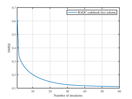
Figure 2: NMSE versus number of iterations for the proposed BCD-based algorithm ($M=64$, $K=12$, $\tau=8$, and $\bar{b}=3$).

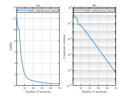
Figure 3: NMSE (a) and constraint violation (b) versus number of outer iterations for the proposed PDD-based algorithm ($M=64$, $K=12$, $\tau=8$, and $\bar{b}=3$).

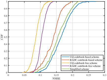
Figure 4: Cumulative distribution function of the NMSE ($M=64$, $K=12$, $\tau=10$, and $\bar{b}=3$).

In Fig. 4, we take a closer look at the cumulative distribution function (CDF) of the NMSE for different schemes. Remarkably, the proposed RADC codebook-free scheme outperforms that of the other competing schemes at any percentile, while the transition of its CDF from 0 to 1 occurs over a smaller range. The results also illustrate that the RADC codebook-based scheme and the simplified scheme yield better NMSE performance than the UQ codebook-based scheme. However, the simplified scheme achieves a suboptimal performance compared to the RADC codebook-based scheme, due to the fact that the pilots are heuristically allocated in advance in the simplified algorithm.

Fig. 5 compares the NMSE of the proposed RADC schemes and the UQ schemes (which fundamentally differ in their bit allocation strategy) as the average number of quantization bits $\bar{b}$ increases. It can be seen for both codebook-free and codebook-based cases, the NMSE of the two schemes coincides for small and large values of $\bar{b}$. However, when $\bar{b}$ (i.e., $3\leq\bar{b}\leq 5$) is moderate, our proposed schemes significantly outperform their corresponding UQ scheme. This fact can be explained as follows: 1) For small values of $\bar{b}$, there is no additional freedom for adapting the allocation of quantization bits to various users’ propagation conditions; 2) For intermediate values of $\bar{b}$, thanks to adaptive quantization bit allocation, the proposed RADC schemes offer added flexibility to select different resolutions to improve channel estimation accuracy; 3) As $\bar{b}$ becomes sufficiently large, the quantization errors caused by the ADCs become less important, and no longer represent the main performance bottleneck of our proposed system.

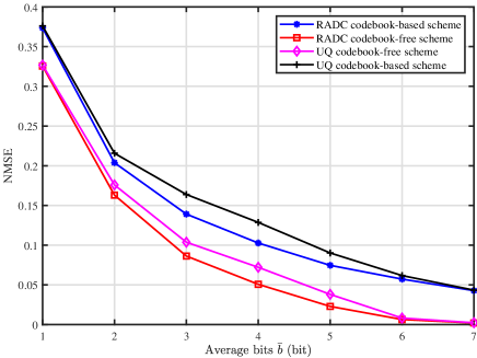
Figure 5: NMSE performance versus the average number of quantization bits $\bar{b}$ ($M=64$, $K=12$, and $\tau=10$).

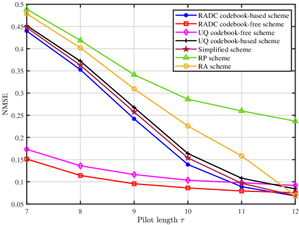
Figure 6: NMSE performance versus the length of pilot sequence $\tau$ ($M=64$, $K=12$, and $\bar{b}=3$).

The effect of the length of pilot sequences $\tau$ on the NMSE performance of different schemes is illustrated in Fig. 6. It can be seen that our proposed RADC codebook-free design yields the best performance among the competing schemes when $\tau\in[7,11]$, while the RADC codebook-based scheme and the simplified scheme provide the lowest NMSE (almost identical) when $\tau=12$. This result is expected because in this case, there are orthogonal pilots to allocate among all the $K=12$ users, which allows significantly better channel estimation accuracy. In general, as the pilot length increases, a noticeable decrease of the channel estimation error can be observed in both RADC schemes. However, the RADC codebook-free scheme holds distinct advantages when short pilots are used, which is of crucial importance for applications with stringent constraints on pilot length.

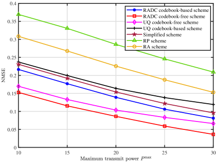
Figure 7: NMSE performance versus the maximum transmit power $P^{\text{max}}$ ($M=64$, $K=12$, $\tau=10$, and $\bar{b}=3$).

Fig. 7 presents the NMSE performance of different schemes versus the maximum transmit power $P^{\text{max}}$. We observe that the NMSE achieved by all schemes is monotonically decreasing with the maximum transmit power. In particular, thanks to the RADC architecture, our proposed RADC codebook-free scheme outperforms its UQ counterpart by a significant margin as the maximum transmit power increases. Furthermore, from the figure, the superiority of the proposed RADC codebook-based and simplified schemes are demonstrated once again. These results validate the effectiveness of the proposed design approach based on the channel estimation minimization.

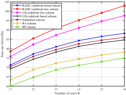
Figure 8: Sum rate performance versus the number users ($M=64$, $\tau=10$, and $\bar{b}=3$).

In Fig. 8, we investigate the sum rate (bits/s/Hz) performance of the various schemes, which is evaluated with the aid of the celebrated precoding algorithm in [52]. As shown in this figure, our proposed RADC codebook-free scheme outperforms the other schemes significantly, which confirms its superiority in serving multiple users. Besides, the RADC codebook-based scheme achieves better performance in transmission than the simplified scheme and the conventional RA scheme, showing that it can strike a better trade-off between transmission rate and complexity.

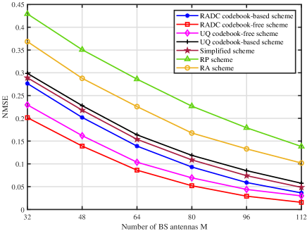
Figure 9: NMSE performance versus the number of antennas at BS ($K=12$, $\tau=10$, and $\bar{b}=3$).

Fig. 9 further shows the NMSE of the channel estimation versus the number of BS antennas $M$. While the NMSE value of all the schemes decreases as the number of BS antennas increases, it is clear that the best performance is achieved by the RADC codebook-free scheme. Moreover, the performance gap between the proposed RADC codebook-based and codebook-free schemes shrinks dramatically as more antennas are being added at the BS. Hence, the proposed joint algorithms for pilot sequence design, bit allocation and hybrid combiner optimization are especially suitable for use in massive MIMO systems with a large number of antennas $M$. The reason is that our proposed scheme can provide significant flexibility over the ADCs with different channel gains and the joint design framework can exploit the difference in channel quality among links for mitigating the multiuser interference as $M$ increases, thereby supporting more favorable uplink training and channel estimation in a cost-effective manner.

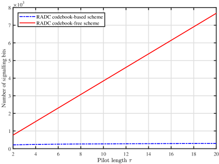
Figure 10: The number of signalling bits versus the length of pilot sequence $\tau$ ($K=24$).

Next, we compare the number of required signalling bits for the feedback of the optimal pilot sequences, for the proposed RADC codebook-based and codebook-free schemes. Let $B$ denotes the number of quantization bits for each element of the codebook-free pilot matrix and of the power vector in the codebook-based pilot scheme. Thus, the number of signalling bits of the RADC codebook-free scheme is given by $2BK\tau$ and that of the RADC codebook-based scheme is $(\lceil\log_{2}\tau\rceil+B)K$, where $\lceil\log_{2}\tau\rceil$ denotes the number of signalling bits required for the codebook feedback of each user. Fig. 10 illustrates the number of signalling bits versus the length $\tau$ of the pilot sequences, where we employ $B=8$ and $K=24$. We can see that the proposed RADC codebook-based scheme can significantly reduce the system feedback overhead compared to the RADC codebook-free scheme. In particular, signalling overhead gap between these two schemes enlarges with the increase of pilot length.

TABLE I: Comparison of Average Mutual Coherence of the Optimal Pilot Sequences in Codebook-Free Schemes.

User	1	2	3	4	5	6	7	8	9	10	11	12
RADC Scheme	0.1327	0.2018	0.2151	0.3563	0.4029	0.5501	0.5322	0.6041	0.6866	0.6736	0.6898	0.6905
UQ Scheme	0.2731	0.5068	0.5626	0.5906	0.6538	0.6282	0.7356	0.7514	0.7673	0.7765	0.7814	0.7818

The average mutual coherence of different users’ pilot sequences obtained in the RADC codebook-free and UQ codebook-free schemes is shown in Table I. We use the factor $\mathrm{c}_{k,i}\triangleq\frac{|\mathbf{s}_{k}^{H}\mathbf{s}_{i}|}{|\mathbf{s}_{k}||\mathbf{s}_{i}|}$ as a measure of the mutual coherence, which reveals the degree of orthogonality among pilot sequences of different users. We label the users based on the strength of channel pathloss, specifically: user 1 encounters the largest pathloss and user 12 encounters the smallest one. It is observed from Table I that both the RADC codebook-free and UQ codebook-free schemes tend to allocate more orthogonal pilots to the users with large pathloss, while assigning less orthogonal pilots to the users with small pathloss. This is reasonable since users with weak channel gain are more easily affected by interference. These results show that codebook-free schemes can take advantage of the knowledge of statistical CSI to in online pilot design in order to enhance the accuracy of channel estimation.

VIII Conclusions

In this paper, we investigated the problem of channel estimation in the uplink massive MIMO systems using RADCs at the BS. We aimed for minimizing the MSE of the Rayleigh fading channel estimates by jointly optimizing the pilot sequences, HAD combiners, and the allocation of ADC quantization bits under practical constraints. To solve such a challenging nonconvex problem, we harnessed the FP technique and introduced some auxiliary variables for transforming the original problem into an equivalent but more manageable form. Then, we developed new BCD-based and PDD-based algorithms for solving the resultant equivalent problem for codebook-free and codebook-based pilot schemes, respectively. Furthermore, we proposed a simplified algorithm for the codebook-based pilot scheme with much reduced complexity. Our simulation results demonstrated the efficiency of the proposed algorithms and their superiority in terms of the MSE and sum rate over the benchmark schemes. It was shown that the RADC codebook-free scheme generally provides better performance than the RADC codebook-based scheme, although the latter entails lower feedback overhead. Hence, the RADC codebook-based scheme is particularly suitable for application scenarios associated with low overhead requirement, while the RADC codebook-free scheme is recommended for applications requiring support for large-scale user access, high channel estimation accuracy and relaxed overhead requirements.

-A Computation of $\hat{\mathbf{h}}_{k}$ in (10) and $\mathrm{MSE}_{k}$ in (11)

The estimate $\hat{\mathbf{h}}_{k}$ of the original channel $\mathbf{h}_{k}$ is obtained by means of the MMSE estimation method based on the observation of $\mathbf{y}_{k}$. Hence, it follows from the standard result in estimation theory [53] that:

$$\hat{\mathbf{h}}_{k}=\mathbb{E}[\mathbf{h}_{k}\mathrm{vec}(\mathbf{y}_{k})^{H}](\mathbb{E}[\mathrm{vec}(\mathbf{y}_{k})\mathrm{vec}(\mathbf{y}_{k})^{H}])^{-1}\mathrm{vec}(\mathbf{y}_{k}).$$ (46)

Substituting (9) into (46), and after some mathematical manipulations, we obtain $\hat{\mathbf{h}}_{k}$ in (10). Denoting the channel estimation error at the BS as $\bm{\varpi}_{k}=\hat{\mathbf{h}}_{k}-\mathbf{h}_{k}$, the corresponding $\mathrm{MSE}_{k}$ is given by $\mathrm{MSE}_{k}=\mathbb{E}[\|\bm{\varpi}_{k}\|^{2}]=\mathbb{E}[\|\hat{\mathbf{h}}_{k}-\mathbf{h}_{k}\|^{2}]$. Thus, using (9), (10) and after some mathematical manipulations, one can obtain

$$\mathrm{MSE}_{k}=\mathrm{tr}(\mathbf{R}_{k}-\mathbf{A}_{k}^{H}\mathbf{B}_{k}^{-1}\mathbf{A}_{k}),$$ (47)

where $\mathbf{A}_{k}=\mathbf{s}_{k}\mathbf{x}_{k}\mathbf{R}_{k}$, and $\mathbf{B}_{k}=\sum_{i}\mathbf{s}_{i}\mathbf{x}_{k}\mathbf{R}_{i}\mathbf{x}_{k}^{H}\mathbf{s}_{i}^{H}+\sigma^{2}\mathbf{x}_{k}\mathbf{x}_{k}^{H}\mathbf{I}_{\tau}+(\mathbf{I}_{\tau}\otimes\mathbf{v}_{k}\mathbf{Q})\mathrm{diag}\Big{(}\sum_{i}(\mathbf{s}_{i}\otimes\mathbf{U})\mathbf{R}_{i}(\mathbf{s}_{i}\otimes\mathbf{U})^{H}+\sigma^{2}\mathbf{I}_{\tau}\otimes\mathbf{U}\mathbf{U}^{\mathbf{H}}\Big{)}(\mathbf{I}_{\tau}\otimes\mathbf{v}_{k}^{H})\succ 0$.

-B Proof of the equivalence between problems (13) and (14) and of the solution $\mathbf{\Gamma}_{k}^{\star}$ in (15)

To prove the equivalence between problem (13) and problem (14), we first introduce
$f_{0_{k}}(\mathbf{b},\mathbf{U},\mathbf{V},\mathbf{S},\bm{\Gamma}_{k})=\!\mathrm{tr}(2\Re\{\mathbf{A}_{k}^{H}\mathbf{\Gamma}_{k}\}\!-\!\mathbf{\Gamma}_{k}^{H}\mathbf{B}_{k}\mathbf{\Gamma}_{k})$. With fixed $\mathbf{b},\mathbf{U},\mathbf{V},\mathbf{S}$ (that is, fixed $\mathbf{A}_{k},\mathbf{B}_{k}$), $f_{0_{k}}$ is concave over the auxiliary variable $\mathbf{\Gamma}_{k}$ and is also a quadratic function of $\mathbf{\Gamma}_{k}$. By applying the first order optimality condition, we can obtain the closed-form solution of problem (14), written as $\mathbf{\Gamma}_{k}^{\star}\!=\!\mathbf{B}_{k}^{-1}\mathbf{A}_{k}$. Upon substitution of $\mathbf{\Gamma}_{k}^{\star}$ into (14), we arrive at the equivalence of problem (13) and problem (14).

$$\mu_{nm} \hat{\mathbf{U}}(n,m)\!=\!\sum_{k}\!\Bigg{(}\!\!(\bar{\mathbf{\Psi}}(n,n)\!+\!\hat{\mathbf{\Psi}}(n,n))\hat{\mathbf{U}}(n,m)\!+\!\sum_{i}\!(\tilde{\mathbf{\Psi}}(n,n)\!+\!\mathbf{\Psi}_{i}(n,n))\hat{\mathbf{U}}(n,m)\mathbf{R}_{i}(m,m)\!\!\Bigg{)}.$$ (54)

$$\varphi_{nm}\!=\!\sum_{k}\!\Bigg{(}\!(\bar{\mathbf{\Psi}}(n,n)\!+\!\hat{\mathbf{\Psi}}(n,n))\hat{\mathbf{U}}(n,m)\!+\!\sum_{i}(\tilde{\mathbf{\Psi}}(n,n)\!+\!\mathbf{\Psi}_{i}(n,n))\hat{\mathbf{U}}(n,m)\mathbf{R}_{i}(m,m)\!\Bigg{)}\!+\!\mathbf{\Phi}(n,m).$$ (55)

-C Quadratic optimization problem with constant-modulus constraints for $\mathbf{U}$

We provide an iterative algorithm to solve the following constant-modulus constrained quadratic optimization problem

$$\underset{\mathbf{U}}{\max} \quad f_{1}(\tilde{\mathbf{b}},\mathbf{U},\mathbf{V},\mathbf{S},\{\mathbf{\Gamma}_{k}\}).$$ (48a)

s.t. $$\quad\ |\mathbf{U}(n,m)|=\frac{1}{\sqrt{M}},\forall{n,m}.$$ (48b)

By introducing $\mathbf{M}=\mathrm{diag}(\mathbf{v}_{k}^{H})$, the cost function $f_{1}(\tilde{\mathbf{b}},\mathbf{U},\mathbf{V},\mathbf{S},\{\mathbf{\Gamma}_{k}\})$ can be rewritten as

$$f_{1} (\tilde{\mathbf{b}},\mathbf{U},\mathbf{V},\mathbf{S},\{\mathbf{\Gamma}_{k}\})$$

$$= \sum_{k}\bigg{(}\mathrm{tr}(2\Re\{\mathbf{R}_{k}\mathbf{x}_{k}^{H}\mathbf{s}_{k}^{H}\mathbf{\Gamma}_{k}\})-\sum_{i}\mathrm{tr}(\mathbf{\Gamma}_{k}^{H}\mathbf{s}_{i}\mathbf{x}_{k}\mathbf{R}_{i}\mathbf{x}_{k}^{H}\mathbf{s}_{i}^{H}\mathbf{\Gamma}_{k})$$

$$-\sum_{i}\mathrm{tr}(\mathrm{diag}(\mathbf{s}_{k}\mathbf{s}_{k}^{H})\mathbf{\Gamma}_{k}\mathbf{\Gamma}_{k}^{H})\mathrm{tr}(\mathbf{Q}\mathbf{U}\mathbf{R}_{i}\mathbf{U}^{H}\mathbf{M}\mathbf{M}^{H})$$

$$-\sigma^{2}\mathrm{tr}(\mathbf{\Gamma}_{k}\mathbf{\Gamma}_{k}^{H})(\mathrm{tr}(\mathbf{Q}\mathbf{U}\mathbf{U}^{H}\mathbf{M}\mathbf{M}^{H})+\mathbf{x}_{k}\mathbf{x}_{k}^{H})\bigg{)}.$$ (49)

We utilize the BCD-type algorithm to tackle problem (48), which is guaranteed to converge to a stationary solution [54]. Specifically, we update each entry of $\mathbf{U}$ once at a time, while keeping the other entries fixed in each step. The function $f_{1}(\tilde{\mathbf{b}},\mathbf{U},\mathbf{V},\mathbf{S},\{\mathbf{\Gamma}_{k}\})$ restricted to a particular entry $\mathbf{U}(n,m)$ can be represented as a quadratic function of $\mathbf{U}(n,m)$ in the form of $\hat{f}(\mathbf{U}(n,m))=2\Re\{\varphi_{nm}^{*}\mathbf{U}(n,m)\}-\mu_{nm}|\mathbf{U}(n,m)|^{2}$, for some complex number $\varphi_{nm}$ and real number $\mu_{nm}$. Then, the problem of maximizing $\hat{f}(\mathbf{U}(n,m))$ with respect to $\mathbf{U}(n,m)$ subject to the constant-modulus constraint is given by

$$\underset{|\mathbf{U}(n,m)|=\frac{1}{\sqrt{M}}}{\max}\quad\hat{f}(\mathbf{U}(n,m)).\\$$ (50)

Considering that $|\mathbf{U}(n,m)|=1/\sqrt{M}$, problem (50) reduces to

$$\underset{|\mathbf{U}(n,m)|=\frac{1}{\sqrt{M}}}{\max}\Re\{\varphi_{nm}^{*}\mathbf{U}(n,m)\}.\\$$ (51)

It follows that the optimal solution of $\mathbf{U}(n,m)$ is given by $\varphi_{nm}/\sqrt{M}|\varphi_{nm}|$. Apparently, we only need to know the value of $\varphi_{nm}$ when updating $\mathbf{U}(n,m)$; below, we show how to obtain $\varphi_{nm}$. On the one hand, we have [55]

$$\left.\frac{\partial{\hat{f}(\mathbf{U}(n,m))}}{\partial{\mathbf{U}^{*}(n,m)}}\right|_{\mathbf{U}(n,m)=\hat{\mathbf{U}}(n,m)}=\varphi_{nm}-\mu_{nm}\hat{\mathbf{U}}(n,m).$$ (52)

On the other hand, let us introduce the following matrix [55]

$$\mathbf{\Phi} =\left.\frac{\partial{f_{1}(\tilde{\mathbf{b}},\mathbf{U},\mathbf{V},\mathbf{S},\{\mathbf{\Gamma}_{k}\})}}{\partial{\mathbf{U}^{*}}}\right|_{\mathbf{U}\!=\!\hat{\mathbf{U}}}$$

$$\!=\!\!\sum_{k}\!\Big{(}\!\mathbf{Q}_{\alpha}\mathbf{v}_{k}^{H}\mathbf{s}_{k}^{H}\mathbf{\Gamma}_{k}\mathbf{R}_{k}\!\Big{)}\!\!-\!\!\sum_{k}\!\Big{(}(\bar{\mathbf{\Psi}}\!+\!\hat{\mathbf{\Psi}})\hat{\mathbf{U}}\!+\!\sum_{i}\!(\tilde{\mathbf{\Psi}}\!+\!\mathbf{\Psi}_{i})\hat{\mathbf{U}}\mathbf{R}_{i}\Big{)},$$ (53)

where $\bar{\mathbf{\Psi}}\!\triangleq\!\sigma^{2}\mathrm{tr}(\mathbf{\Gamma}_{k}\mathbf{\Gamma}_{k}^{H})\mathbf{Q}_{\alpha}\mathbf{v}_{k}^{H}\mathbf{v}_{k}\mathbf{Q}_{\alpha}$, $\hat{\mathbf{\Psi}}\!\triangleq\!\sigma^{2}\mathrm{tr}(\mathbf{\Gamma}_{k}\mathbf{\Gamma}_{k}^{H})\mathbf{M}\mathbf{M}^{H}\mathbf{Q}$, $\tilde{\mathbf{\Psi}}\!\triangleq\!\mathrm{tr}(\mathrm{diag}(\mathbf{s}_{k}\mathbf{s}_{k}^{H})\mathbf{\Gamma}_{k}\mathbf{\Gamma}_{k}^{H})\mathbf{M}\mathbf{M}^{H}\mathbf{Q}$, and $\mathbf{\Psi}_{i}\triangleq\mathbf{Q}_{\alpha}\mathbf{v}_{k}^{H}\mathbf{s}_{i}^{H}\mathbf{\Gamma}_{k}\mathbf{\Gamma}_{k}^{H}\mathbf{s}_{i}\mathbf{v}_{k}\mathbf{Q}_{\alpha}$. Combining (52) and (-C), we obtain $\mathbf{\Phi}(n,m)=\varphi_{nm}-\mu_{nm}\hat{\mathbf{U}}(n,m)$. By expanding $[(\bar{\mathbf{\Psi}}\!+\!\hat{\mathbf{\Psi}})\hat{\mathbf{U}}\!+\!\!\sum_{i}(\tilde{\mathbf{\Psi}}+\mathbf{\Psi}_{i})\hat{\mathbf{U}}\mathbf{R}_{i}](n,m)$ and examining the coefficient of $\hat{\mathbf{U}}(n,m)$, we find (54) displayed at the top of this page. Therefore, the value of $\varphi_{nm}$ is determined as (55), shown at the top of this page.

-D Proof of Theorem 1

We focus on the proof of Theorem 1, i.e., the convergence of Algorithm 1. It is seen that each subproblem in the proposed BCD-based Algorithm 1 is guaranteed to converge to its stationary point. Specifically, the subproblem with respect to $\mathbf{U}$, $\mathbf{V}$ and $\mathbf{S}$ can be globally solved, respectively, and the solutions satisfy the optimality conditions. As for the subproblem for $\tilde{\mathbf{b}}$ (the relaxation variable of $\mathbf{b}$), we leverage the SCA method and construct the concave surrogate function $\bar{f}^{t}(\tilde{\mathbf{b}})$ to approximate the nonconcave objective function $f_{1}(\tilde{\mathbf{b}})$. Then, the complex nonconcave optimization subproblem (17) is transformed into a concave subproblem (20) with guaranteed convergence. The valid surrogate function $\bar{f}^{t}(\tilde{\mathbf{b}})$ and $f_{1}(\tilde{\mathbf{b}})$ have the same value and gradient at point $\tilde{\mathbf{b}}^{t}$ which follows from the SCA theory [56]. Consequently, subproblem (17) and subproblem (20) will share the same stationary point.

With objective function value of each subproblem nondecreasing and guaranteed to converge to its stationary point and according to Proposition 2.7.1 (Convergence of BCD) in [54], Algorithm 1 is guaranteed to converge to a stationary point of problem (14). Furthermore, based on Lemma 1, problem (13) and problem (14) can share the same stationary points. Therefore, Algorithm 1 is guaranteed to converge to a stationary point of problem (13).

References

- [1] T. L. Marzetta, “Noncooperative cellular wireless with unlimited numbers of base station antennas,” IEEE Trans. Wireless Commun., vol. 9, no. 11, pp. 3590-3600, Nov. 2010.
- [2] F. Rusek, D. Persson, B. K. Lau, E. G. Larsson, T. L. Marzetta, and F. Tufvesson, “Scaling up MIMO: Opportunities and challenges with very large arrays,” IEEE Signal Process. Mag., vol. 30, no. 1, pp. 40-60, Jan. 2013.
- [3] L. Lu, G. Y. Li, A. L. Swindlehurst, A. Ashikhmin, and R. Zhang, “An overview of massive MIMO: Benefits and challenges,” IEEE J. Sel. Topics Signal Process., vol. 8, no. 5, pp. 742-758, Oct. 2014.
- [4] R. H. Walden, “Analog-to-digital converter survey and analysis,” IEEE J. Sel. Areas Commun., vol. 17, no. 4, pp. 539-550, Apr. 1999.
- [5] L. Bin, T. W. Rondeau, J. H. Reed, and C. W. Bostian, “Analog-to-digital converters,” IEEE Signal Process. Mag., vol. 22, no. 6, pp. 69-77, Nov. 2005.
- [6] I. Ahmed, H. Khammari, A. Shahid, A. Musa, K. S. Kim, E. De Poorter, and I. Moerman, “A survey on hybrid beamforming techniques in 5G: Architecture and system model perspectives,” IEEE Commun. Surveys Tuts., vol. 20, no. 4, pp. 3060-3097, 4th Quart., 2018.
- [7] C. Huang, L. Liu, C. Yuen, and S. Sun, “Iterative channel estimation using LSE and sparse message passing for mmwave MIMO systems,” IEEE Trans. Signal Process., vol. 67, no. 1, pp. 245-259, Jan. 2019.
- [8] X. Yu, J. Shen, J. Zhang, and K. B. Letaief, “Alternating minimization algorithms for hybrid precoding in millimeter wave MIMO systems,” IEEE J. Sel. Topics Signal Process., vol. 10, no. 3, pp. 485-500, Apr. 2016.
- [9] F. Sohrabi and W. Yu, “Hybrid analog and digital beamforming for OFDM-based large-scale MIMO systems,” in Proc. IEEE 17th Int. Workshop Signal Process. Adv. Wireless Commun., Edinburgh, U.K., 2016, pp. 1-5.
- [10] X. Gao, L. Dai, S. Han, C. L. I, and R. W. Heath, “Energy-efficient hybrid analog and digital precoding for mmwave MIMO systems with large antenna arrays,” IEEE J. Sel. Areas Commun., vol. 34, no. 4, pp. 998-1009, Apr. 2016.
- [11] G. Zhu, K. Huang, V. K. N. Lau, B. Xia, X. Li, and S. Zhang, “Hybrid beamforming via the Kronecker decomposition for the millimeter-wave massive MIMO systems,” IEEE J. Sel. Areas Commun., vol. 35, no. 9, pp. 2097-2114, Sep. 2017.
- [12] X. Yu, J. Zhang, and K. B. Letaief, “A hardware-efficient analog network structure for hybrid precoding in millimeter wave systems,” IEEE J. Sel. Topics Signal Process., vol. 12, no. 2, pp. 282-297, May 2018.
- [13] X. Xue, Y. Wang, L. Yang, J. Shi, and Z. Li, “Energy-efficient hybrid precoding for massive MIMO mmWave systems with a fully-adaptive-connected structure,” IEEE Trans. Commun., vol. 68, no. 6, pp. 3521-3535, Jun. 2020.
- [14] X. Zhu, Z. Wang, L. Dai, and Q. Wang, “Adaptive hybrid precoding for multiuser massive MIMO,” IEEE Commun. Lett., vol. 20, no. 4, pp. 776-779, Apr. 2016.
- [15] X. Xue, Y. Wang, L. Dai, and C. Masouros, “Relay hybrid precoding design in millimeter-wave massive MIMO systems,” IEEE Trans. Signal Process., vol. 66, no. 8, pp. 2011-2026, Apr. 2018.
- [16] Y. Cai, Y. Xu, Q. Shi, B. Champagne, and L. Hanzo, “Robust joint hybrid transceiver design for millimeter wave full-duplex MIMO relay systems,” IEEE Trans. Wireless Commun., vol. 18, no. 2, pp. 1199-1215, Feb. 2019.
- [17] C. Lin and G. Y. Li, “Terahertz communications: An array-of-subarrays solution,” IEEE Commun. Mag., vol. 54, no. 12, pp. 124-131, Dec. 2016.
- [18] J. Mo and R. W. Heath, “Capacity analysis of one-bit quantized MIMO systems with transmitter channel state information,” IEEE Trans. Signal Process., vol. 63, no. 20, pp. 5498-5512, Oct. 2015.
- [19] P. Dong, H. Zhang, W. Xu, G. Y. Li, and X. You, “Performance analysis of multiuser massive MIMO with spatially correlated channels using low-precision ADC,” IEEE Commun. Lett., vol. 22, no. 1, pp. 205-208, Jan. 2018.
- [20] J. Mo, A. Alkhateeb, S. Abu-Surra, and R. W. Heath, “Hybrid architectures with few-bit ADC receivers: Achievable rates and enrgy-rate tradeoffs,” IEEE Trans. Wireless Commun., vol. 16, no. 4, pp. 2274-2287, Apr. 2017.
- [21] Y. Wang, X. Chen, Y. Cai, and L. Hanzo, “Stochastic hybrid combining design for quantized massive MIMO systems,” IEEE Trans. Veh. Technol., vol. 69, no. 12, pp. 16224-16229, Dec. 2020.
- [22] J. Choi, G. Lee, and B. L. Evans, “Two-stage analog combining in hybrid beamforming systems with low-resolution ADCs,” IEEE Trans. Signal Process., vol. 67, no. 9, pp. 2410-2425, May 2019.
- [23] K. Roth and J. A. Nossek, “Achievable rate and energy efficiency of hybrid and digital beamforming receivers with low resolution ADC,” IEEE J. Sel. Areas Commun., vol. 35, no. 9, pp. 2056-2068, Sept. 2017.
- [24] H. Sheng, X. Chen, K. Shen, X. Zhai, A. Liu, and M. Zhao, “Energy efficiency optimization for beamspace massive MIMO systems with low-resolution ADCs,” in Proc. IEEE Wireless Commun. Netw. Conf. (WCNC), Seoul, Korea, May 2020, pp. 1-7.
- [25] K. Roth, H. Pirzadeh, A. L. Swindlehurst, and J. A. Nossek, “A comparison of hybrid beamforming and digital beamforming with low-resolution ADCs for multiple users and imperfect CSI,” IEEE J. Sel. Topics Signal Process., vol. 12, no. 3, pp. 484-498, Jun. 2018.
- [26] A. Kaushik, E. Vlachos, J. Thompson, and A. Perelli, “Efficient channel estimation in millimeter wave hybrid MIMO systems with low resolution ADCs,” in 26th European Signal Processing Conference (EUSIPCO), Rome, 2018, pp. 1825-1829.
- [27] H. He, C. Wen, and S. Jin, “Bayesian optimal data detector for hybrid mmWave MIMO-OFDM systems with low-resolution ADCs,” IEEE J. Sel. Topics Signal Process., vol. 12, no. 3, pp. 469-483, Jun. 2018.
- [28] J. Park, S. Park, A. Yazdan, and R. W. Heath, “Optimization of mixed-ADC multi-antenna systems for Cloud-RAN deployments,” IEEE Trans. Commun., vol. 65, no. 9, pp. 3962-3975, Sept. 2017.
- [29] J. Choi, B. L. Evans, and A. Gatherer, “Resolution-adaptive hybrid MIMO architectures for millimeter wave communications,” IEEE Trans. Signal Process., vol. 65, no. 23, pp. 6201-6216, Dec. 2017.
- [30] K. Nguyen, Q. Vu, L. Tran, and M. Juntti, “Energy-efficient bit allocation for resolution-adaptive ADC in multiuser large-scale MIMO systems: Global optimality,” in IEEE Int. Conf. Acoust., Speech, and Signal Process.(ICASSP), Barcelona, Spain, 2020, pp. 5130-5134.
- [31] A. Kaushik, C. Tsinos, E. Vlachos, and J. Thompson, “Energy efficient ADC bit allocation and hybrid combining for millimeter wave MIMO systems,” in 2019 IEEE Global Communications Conference (GLOBECOM), 2019, pp. 1-6.
- [32] H. Sheng, X. Chen, X. Zhai, A. Liu, and M. Zhao, “Energy efficiency optimization for millimeter wave system with resolution-adaptive ADCs,” IEEE Wireless Commun. Lett, vol. 9, no. 9, pp. 1519-1523, Sept. 2020.
- [33] X. Chen, Y. Cai, A. Liu, and L. Hanzo, “Joint user scheduling and resource allocation for millimeter wave systems relying on adaptive-resolution ADCs,” [Online]. Available: https://arxiv.org/abs/2009.12482
- [34] Y. Xiong, “Achievable rates for massive MIMO relaying systems with variable-bit ADCs/DACs,” IEEE Commun. Lett., vol. 24, no. 5, pp. 991-994, May 2020.
- [35] Y. Xiu, J. Zhao, E. Basar, M. Di Renzo, W. Sun, G. Gui, and N. Wei, “Uplink achievable rate maximization for reconfigurable intelligent surface aided millimeter wave systems with resolution-adaptive ADCs,” IEEE Wireless Commun. Lett, vol. 10, no. 8, pp. 1608-1612, Aug. 2021.
- [36] H. V. Cheng, E. Björnson, and E. G. Larsson, “Optimal pilot and payload power control in single-cell massive MIMO systems,” IEEE Trans. Signal Process., vol. 65, no. 9, pp. 2363-2378, May 2017.
- [37] L. You, X. Gao, X. G. Xia, N. Ma, and Y. Peng, “Pilot reuse for massive MIMO transmission over spatially correlated Rayleigh fading channels,” IEEE Trans. Wireless Commun., vol. 14, no. 6, pp. 3352-3366, Jun. 2015.
- [38] K. Shen, H. V. Cheng, X. Chen, Y. C. Eldar, and W. Yu, “Enhanced channel estimation in massive MIMO via coordinated pilot design,” IEEE Trans. Commun., vol. 68, no. 11, pp. 6872-6885, Nov. 2018.
- [39] S. Park, O. Simeone, Y. C. Eldar, and E. Erkip, “Optimizing pilots and analog processing for channel estimation in cell-free massive MIMO with one-bit ADCs,” in IEEE Workshop Signal Process. Advances Wireless Commun. (SPAWC), 2018, pp. 1-5.
- [40] X. Chen, A. Liu, W. Yu, H. V. Cheng, K. Shen, and M. Zhao, “Distributed pilot design for massive connectivity in cellular networks,” in IEEE Global Commun. Conf. (GLOBECOM), HI, USA, 2019, pp. 1-6.
- [41] Z. Chen, F. Sohrabi, and W. Yu, “Sparse activity detection for massive connectivity,” IEEE Trans. Signal Process., vol. 66, no. 7, pp. 1890-1904, Apr. 2018.
- [42] S. S. Ioushua and Y. C. Eldar, “Pilot sequence design for mitigating pilot contamination with reduced RF chains,” IEEE Trans. Commun., vol. 68, no. 6, pp. 3536-3549, Jun. 2020.
- [43] K. Shen, W. Yu, L. Zhao, and D. P. Palomar, “Optimization of MIMO device-to-device networks via matrix fractional programming: A minorization-maximization approach,” IEEE/ACM Trans. Netw., vol. 27, no. 5, pp. 2164-2177, Oct. 2019.
- [44] L. Liu and R. Zhang, “Optimized uplink transmission in multi-antenna C-RAN with spatial compression and forward,” IEEE Trans. Signal Process., vol. 63, no. 19, pp. 5083-5095, Oct. 2015.
- [45] M. Grant and S. Boyd, “CVX: Matlab software for disciplined convex programming, version 2.1,” http://cvxr.com/cvx, Mar. 2014.
- [46] Q. Shi and M. Hong, “Spectral efficiency optimization for mmWave multiuser MIMO systems,” IEEE J. Sel. Toptics Signal Process., vol. 12, no. 3, pp. 455-468, Jun. 2018.
- [47] Q. Shi and M. Hong, “Penalty dual decomposition method for nonsmooth nonconvex optimization-Part I: Algorithms and convergence analysis,” IEEE Trans. Signal Process., vol. 68, pp. 4108-4122, Jun. 2020.
- [48] F. Cui, Y. Cai, Z. Qin, M. Zhao, and G. Y. Li, “Multiple access for mobile-UAV enabled networks: Joint trajectory design and resource allocation,” IEEE Trans. Commun., vol. 67, no. 7, pp. 4980-4994, Jul. 2019.
- [49] Technical Specification Group Radio Access Network: Further Advancements for E-UTRA Physical Layer Aspects, 3GPP TR 36.814. [Online]. Available: http://www.3gpp.org
- [50] E. Björnson, M. Matthaiou, A. Pitarokoilis, and M. Debbah, “Distributed massive MIMO in cellular networks: Impact of imperfect hardware and number of oscillators,” in Proc. 23rd Eur. Signal Process. Conf., Sept. 2015, pp. 2436-2440.
- [51] L. Wei, C. Huang, G. C. Alexandropoulos, C. Yuen, Z. Zhang, and M. Debbah, “Channel estimation for RIS-empowered multi-user MISO wireless communications,” IEEE Trans. Commun., vol. 69, no. 6, pp. 4144-4157, Jun. 2021.
- [52] Q. Shi, M. Razaviyayn, Z.-Q. Luo, and C. He, “An iteratively weighted MMSE approach to distributed sum-utility maximization for a MIMO interfering broadcast channel,” IEEE Trans. Signal Process., vol. 59, no. 9, pp. 4331-4340, Sept. 2011.
- [53] T. Kailath, A. H. Sayed, and B. Hassibi, Linear Estimation. Prentice Hall, 2000.
- [54] D. Bertsekas, Nonlinear Programming, 2nd ed. Belmont, MA: Athena Scientific, 1999.
-
[55]
K. B. Petersen and M. S. Pedersen, “The matrix cookbook,” Nov. 2012. [Online].
Available:https://www.math.uwaterloo.ca/hwolkowi/matrixcookbook.pdf - [56] M. Razaviyayn, “Successive convex approximation: Analysis and applications,” Ph.D. dissertation, University of Minnesota, 2014.