$C^{1}$-VEM for some variants of the Cahn-Hilliard equation: a numerical exploration

Abstract

We consider the $C^{1}$-Virtual Element Method (VEM) for the conforming numerical approximation of some variants of the Cahn-Hilliard equation on polygonal meshes. In particular, we focus on the discretization of the advective Cahn-Hilliard problem and the Cahn-Hilliard inpainting problem. We present the numerical approximation and several numerical results to assess the efficacy of the proposed methodology.

Keywords: Virtual element method, Polytopal meshes, Fourth order problems, Cahn-Hilliard equation, Impainting, Parallel computing.

1 Introduction

The Cahn-Hilliard equation, which is a fourth-order nonlinear parabolic problem, was initially introduced as a diffusive interface model to characterize the phase segregation of binary alloys at constant temperature [30]. Compared to sharp-interface models, where the individual interfaces need to be explicitly tracked, the advantage of a diffuse-interface approach is that topological changes are automatically handled, since interfaces are treated in a diffuse manner thanks to the introduction of a parameter which, varying continuously, accounts for the different material phases and/or the concentration of the different components. Since the seminal paper by Cahn and Hilliard, several different variants have been studied (see, e.g., the book [67] and the references therein) covering a wide spectrum of applications. Here we mention, for example, the modeling and simulation of solidification processes, spinodal decomposition, coarsening of precipitate phases, shape memory effects, re-crystallisation, dislocation dynamics [33, 41, 68, 74], wettability [47], diblock copolymer [75, 73], tumor growth [2, 48, 53, 78, 31], image inpainting [23, 22], crystal growth [37, 42, 76, 51] and crack propagation [66, 60, 24].

In the last decades, different numerical techniques have been utilized to solve the Cahn-Hilliard equation and its variants, including finite difference, finite element, and spectral methods. A crucial difficulty in designing numerical schemes is that these equations typically involve spatial differential operators that are higher than second-order. Therefore, standard conforming $C^{0}$ Finite Element Methods (FEMs) are ruled out and approximation spaces with higher regularity are required. However, the construction of such approximation spaces with higher regularity is deemed a difficult task because it requires a set of basis functions with such a global regularity. Examples in this direction can be found all along the history of finite elements: from the oldest works in the sixties of the last century, e.g., [9, 21, 35] to the most recent attempts in [79, 80, 56, 55]. Despite its intrinsic difficulty, designing approximations with global $C^{1}$ or higher regularity is still a major research topic. In the literature there is a limited number of works addressing the solution of the Cahn-Hilliard equation by the $C^{1}$-FEM, see [40, 39]. To circumvent the well known difficulty met in the implementation of $C^{1}$-FEMs, another possibility is the use of non-conforming (see, e.g., [38]) or discontinuous (see, e.g., [77, 43]) methods; obviously in such cases the discrete solution will not satisfy $C^{1}$ regularity.

Alternatively, the Cahh-Hilliard problem can be split into a coupled of lower-order differential equations and mixed formulation can be employed for discretization at the expense of introducing additional unknowns, see, e.g., [46, 58, 10, 62, 32, 64]. Recently, in [52] isogeometric analysis has been employed to discretize the Cahn-Hilliard problem, whereas in [63] the same approach has been used to discretize the advective Cahn-Hilliard equation. A remarkable feature of this methodology is that the approximation spaces exhibit higher-order continuity properties, thus avoiding the use of mixed formulations. More recently, in [6] the $C^{1}$-Virtual Element Method (VEM) has been employed to discretize the Cahn-Hilliard equation on polygonal meshes, employing highly regular conforming approximation spaces, thus circumventing the introduction of additional variables typical of mixed formulations.

Roughly speaking, the VEM is a Galerkin-type projection method that generalize the finite element method, which was originally designed for simplicial and quadrilateral/hexahedral meshes, to polygonal/polyhedral (polytopal, for short) meshes. The VEM has been originally introduced in [13] and does not require the explicit knowledge of the basis functions spanning the approximation space. The functions that belong to such approximation spaces are dubbed as “virtual” as they are never really computed, with the noteworthy exception of a subspace of polynomials that are indeed used in the formulation and implementation of the method. The virtual element functions are uniquely characterized by a set of values, the so called degrees of freedom. The VEM can then be implemented using only the degrees of freedom and the polynomial part of the approximation space. The crucial idea behind the VEM is that the elemental approximation space is defined elementwise as the solution of a partial differential equation. Then the global approximation space is obtained by globally “gluing” the local spaces in an arbitrary highly regular conforming way. Thus, the virtual element “paradigm” provides a major breakthrough as it allows to obtain highly-regular Galerkin methods, and the construction of numerical approximation sof any order of accuracy on unstructured two-dimensional and three-dimensional meshes made by general polytopal elements.

The first works proposing a $C^{1}$-regular conforming VEM addressed the classical plate bending problems [29, 34], second-order elliptic problems [16, 17], and the nonlinear Cahn-Hilliard equation [6]. More recently, highly regular virtual element spaces were considered for the von Kármán equation modeling the deformation of very thin plates [65], geostrophic equations [70] and fourth-order subdiffusion equations [61], two-dimensional plate vibration problems of Kirchhoff plates [69], transmission eigenvalue problems [71], and fourth-order plate buckling eigenvalue problems [72]. In [8] the highly-regular conforming VEM for the two-dimensional polyharmonic problem $(-\Delta)^{p_{1}}u=f$, $p_{1}\geq 1$ has been proposed. The VEM is based on an approximation space that locally contains polynomials of degree $r\geq 2p_{1}-1$ and has a global $H^{p_{1}}$ regularity. In [7], this formulation has been extended to a virtual element space that can have arbitrary regularity $p_{2}\geq p_{1}\geq 1$ and contains polynomials of degree $r\geq p_{2}$. VEMs for three-dimensional problems are also available for the fourth-order linear elliptic equations [15] (see also [26]), and highly-regular conforming VEM in any dimension has been proposed in [57].

In this paper, hinging upon the use of $C^{1}$-VEM, we study the conforming virtual element approximation on polygonal meshes of two variants of the Cahn-Hilliard equation, namely the Advective Cahn-Hilliard (ACH) problem and the Cahn-Hilliard Inpainting problem (CHI). Those variants have been selected both for their relevance in applications and for the presence, with respect to the classical Cahn-Hilliard equation, of the additional convective term in the ACH problem and the reaction term in the CHI problem. The numerical treatment of those terms is new in the context of the conforming virtual element discretization of Cahn-Hilliard equations. It is also worth mentioning that the numerical treatment of the advective Cahn-Hilliard represents an important preliminary step to tackle in future works the virtual element approximation of more complicated problems, as the convective nonlocal Cahn-Hilliard (see, e.g., [36]) or the Navier-Stokes-Cahn-Hilliard problem (see, e.g., [49, 50] and [12, 45, 59]).

The paper is organized as follows. In Section 2 we introduce the continuous problems, whereas in Section 3 we present their conforming virtual element approximation. In Section 4 we collect and discuss several numerical results to show the efficacy of our discretization methodology. Finally, in Section 5 we draw some conclusions.

Notation. Throughout the paper, we will follow the usual notation for Sobolev spaces and norms [1]. Hence, for an open bounded domain $\omega$, the norms in the spaces $W^{s}_{p}(\omega)$ and $L^{p}(\omega)$ are denoted by $\|{\cdot}\|_{W^{s}_{p}(\omega)}$ and $\|{\cdot}\|_{L^{p}(\omega)}$, respectively. The norm and seminorm in $H^{s}(\omega)$, $s\geq 1$, are denoted by $\|{\cdot}\|_{s,\omega}$ and $|{\cdot}|_{s,\omega}$, respectively. The $L^{2}$-inner product and the $L^{2}$-norm are denoted by $(\cdot,\cdot)_{\omega}$ and $\|\cdot\|_{\omega}$, respectively. The subscript $\omega$ may be omitted when $\omega$ is the whole computational domain $\Omega$. We denote with $\boldsymbol{x}=(x_{1},\,x_{2})$ the independent variable. With the usual notation the symbols $\nabla$, $\Delta$, $\Delta^{2}$, $D^{2}$ denote the gradient, the laplacian, the bilaplacian and the Hessian for (regular enough) scalar functions, whereas $\partial_{t}$ denotes the derivative with respect to the time variable.

2 Continuous problems

In this Section we introduce the two variants of the classical Cahn-Hilliard problem, whose numerical discretization will be addressed in the sequel of this paper. More specifically, we consider the Advective Cahn-Hilliard problem and the Cahn-Hilliard Impainting problem. For each variant, we provide the weak formulation that will the basis for the construction of the virtual element discretization.

Let $\Omega\subset\mathbb{R}^{2}$ be an open bounded domain. Let $\psi:\mathbb{R}\to\mathbb{R}$ with $\psi(x)=(1-x^{2})^{2}/4$ and let $\phi(x)=\psi^{\prime}(x)$, we consider the following two variants of the Cahn-Hilliard problem, where $\gamma\in{\mathbb{R}}^{+}$, $0<\gamma\ll 1$, represents the interface parameter.

Advective Cahn-Hilliard problem. For a given final time $T>0$, find $c(x,t):\Omega\times[0,T]\rightarrow{\mathbb{R}}$ such that:

$$\left\{\begin{aligned} &\partial_{t}c-\frac{1}{\text{Pe}}\Delta\big{(}\phi(c)-\gamma^{2}\Delta c\big{)}+{\rm div}(\boldsymbol{u}c)=0&&\textrm{ in }\Omega\times(0,T],\\ &c(\cdot,0)=c_{0}(\cdot)&&\textrm{ in }\Omega,\\ &\partial_{\bf n}c={\partial_{\bf n}}\big{(}\phi(c)-\gamma^{2}\Delta c\big{)}=0&&\textrm{ on }\partial\Omega\times(0,T],\end{aligned}\right.$$ (1)

where $\partial_{\boldsymbol{n}}$ denotes the (outward) normal derivative and Pe is a positive constant. We note that on the boundary of the domain we impose no-flux type condition both on $c$ and on the so-called chemical potential $\phi(c)-\gamma^{2}\Delta c$. Finally, $\boldsymbol{u}\in H({\rm div},\Omega)\cap[C^{0}(\Omega)]^{2}$ is a given function such that ${\rm div}\boldsymbol{u}=0$ in $\Omega$ and $\boldsymbol{u}\cdot\boldsymbol{n}=0$ on $\partial\Omega$. Here

$$H({\rm div},\Omega)=\{\boldsymbol{v}\in[L^{2}(\Omega)]^{2}:{\rm div}\boldsymbol{v}\in L^{2}(\Omega)\}\,.$$

Cahn-Hilliard inpainting problem. Let $f$ be a given binary image and $D\subset\Omega$ be the inpainting domain. For a given final time $T>0$, find $c(x,t):\Omega\times[0,T]\rightarrow{\mathbb{R}}$ such that:

$$\left\{\begin{aligned} &\partial_{t}c-\Delta\big{(}\frac{1}{\gamma}\phi(c)-\gamma\Delta c\big{)}+\lambda(x)(f-c)=0&&\textrm{ in }\Omega\times(0,T],\\ &c(\cdot,0)=c_{0}(\cdot)&&\textrm{ in }\Omega,\\ &\partial_{\bf n}c={\partial_{\bf n}}\big{(}\frac{1}{\gamma}\phi(c)-\gamma\Delta c\big{)}=0&&\textrm{ on }\partial\Omega\times(0,T],\end{aligned}\right.$$ (2)

where

$$\lambda(x)=\left\{\begin{aligned} &\lambda_{0},\quad&\boldsymbol{x}\in\Omega\setminus D,\\ &0,\quad&\boldsymbol{x}\in D,\end{aligned}\right.$$

$\lambda_{0}$ being a positive parameter. See, e.g., [23, 22] for more details on the model.

We now briefly introduce the variational formulations of (1) and (2) that will be used to derive the virtual element discretizations. To this aim, we preliminary define the following bilinear forms

$$a^{D^{2}}(v,w)=\int_{\Omega}(D^{2}v):(D^{2}w)\,{\rm d}\Omega \forall v,w\in H^{2}(\Omega),$$ (3)

$$a^{0}(v,w)=\int_{\Omega}v\,w\,{\rm d}\Omega \forall v,w\in L^{2}(\Omega),$$

$$b(v,w)=\int_{\Omega}{\bf u}\cdot\nabla v\ w\,{\rm d}\Omega \forall v,w\in H^{1}(\Omega),$$

and the semi-linear forms

$$l(f;v,w)=\int_{\Omega}\lambda(f-v)w\,{\rm d}\Omega \forall v,w\in L^{2}(\Omega)\,,$$ (4)

$$r(z;v,w)=\int_{\Omega}\phi^{\prime}(z)\nabla v\cdot\nabla w\,{\rm d}\Omega \forall z,v,w\in H^{2}(\Omega)\,.$$

Finally, we introduce the space

$$V=\big{\{}v\in H^{2}(\Omega)\>:\>\partial_{\bf n}{v}=0\textrm{ on }\partial\Omega\big{\}}.$$ (5)

The weak formulation of problem (1) reads as follows: find $c(\cdot,t)\in V$ s.t.

$$\left\{\begin{aligned} &a^{0}(\partial_{t}c,v)+\frac{\gamma^{2}}{\text{Pe}}a^{D^{2}}(c,v)+\frac{1}{\text{Pe}}r(c;c,v)+b(c,v)=0\quad\forall v\in V,\\ &c(\cdot,0)=c_{0}\,.\end{aligned}\right.$$ (6)

Similarly, the weak formulation of problem (2) reads as follows: find $c(\cdot,t)\in V$ s.t.

$$\left\{\begin{aligned} &a^{0}(\partial_{t}c,v)+{\gamma}a^{D^{2}}(c,v)+\frac{1}{\gamma}r(c;c,v)+l(f;c,v)=0\quad\forall v\in V,\\ &c(\cdot,0)=c_{0}\,.\end{aligned}\right.$$ (7)

3 Virtual element discretization

In this Section we describe the virtual element discretization of problems (6)-(7) on computational meshes made of general polygons. In particular, in Section 3.1 we introduce the assumptions on the regularity of the polygonal mesh together with the definition of crucial projector operators that will be fundamental in the construction of the virtual element discretization. In Section 3.2 we describe the $C^{1}$-Virtual Element spaces that will of paramount importance to guarantee a conforming approximation of the Cahn-Hilliard problems. Finally, in Section 3.4 we introduce the semi-discrete in space virtual element discretization of (6)-(7) together with a fully discrete scheme based on the use of the backward Euler method for time discretization.

3.1 Mesh assumptions and polynomial projections

From now on, we will denote with $E$ a general polygon, having $n_{e}$ edges $e$, moreover $|E|$ and $h_{E}$ will denote the area and the diameter of $E$, respectively. Let $\{\Omega_{h}\}_{h}$ be a sequence of decompositions of $\Omega$ into general polygons $E$, where the granularity $h$ is defined as $h=\sup_{E\in\Omega_{h}}h_{E}$. We suppose that $\{\Omega_{h}\}_{h}$ fulfills the following assumption:
(A1) Mesh assumption. There exists a positive constant $\rho$ such that for any $E\in\{\Omega_{h}\}_{h}$

• Any $E\in\{\Omega_{h}\}_{h}$ is star-shaped with respect to a ball $B_{E}$ of radius $\geq\,\rho\,h_{E}$;

• Any edge $e$ of any $E\in\{\Omega_{h}\}_{h}$ has length $\geq\,\rho\,h_{E}$.

We remark that the hypotheses above, though not too restrictive in many practical cases, could possibly be further relaxed, combining the present analysis with the studies in [20, 25, 27].

Referring to Problem (7), we assume that for any $h$ there exists $D_{h}\subseteq\Omega_{h}$ such that $D_{h}$ is a decomposition of $D$, i.e. $\Omega_{h}$ matches with the subdivision of $\Omega$ into $D$ and $\Omega\setminus D$.

We denote with $\Sigma_{h}$ the set of all the mesh edges and for any $E\in\Omega_{h}$ we denote with $\Sigma_{h}^{E}$ the set of the edges of $E$. Furthermore for any mesh vertex $\boldsymbol{\xi}$ we denote with $h_{\boldsymbol{\xi}}$ the average of the diameters of the elements having $\boldsymbol{\xi}$ as a vertex. The total number of vertexes, edges and elements in the decomposition $\Omega_{h}$ are denoted by $N_{V}$, $N_{e}$ and $N_{P}$, respectively.

Using standard VEM notations, for any mesh object $\omega\in\Omega_{h}\cup\Sigma_{h}$ and for any $n\in\mathbb{N}$ let us introduce the space $\mathbb{P}_{n}(\omega)$ to be the space of polynomials defined on $\omega$ of degree $\leq n$ (with the extended notation $\mathbb{P}_{m}(\omega)=\{0\}$ for any negative integer $m$). Moreover, $\widehat{\mathbb{P}}_{n\setminus m}(\omega)=\mathbb{P}_{n}(\omega)\setminus\mathbb{P}_{m}(\omega)$, for $m<n$, denotes the polynomials in $\mathbb{P}_{n}(\omega)$ with monomials of degree strictly greater than $m$. Finally, we introduce the broken polynomial space

$$\mathbb{P}_{n}(\Omega_{h})=\{q\in L^{2}(\Omega)\quad\text{s.t.}\quad q|_{E}\in\mathbb{P}_{n}(E)\quad\text{for all $E\in\Omega_{h}$}\}\,.$$

For any non-negative $s\in\mathbb{R}$ let us introduce the broken space:

$$H^{s}(\Omega_{h})=\{v\in L^{2}(\Omega)\quad\text{s.t.}\quad v|_{E}\in H^{s}(E)\quad\text{for all $E\in\Omega_{h}$}\}\,.$$

Furthermore, we introduce the following notation: let $\{\mathcal{X}^{E}\}_{E\in\Omega_{h}}$ be a family of forms $\mathcal{X}^{E}\colon\prod_{j=1}^{\ell}H^{s_{j}}(E)\to\mathbb{R}$, then we define

$$\mathcal{X}\colon\prod_{j=1}^{\ell}H^{s_{j}}(\Omega_{h})\to\mathbb{R}\,,\quad\mathcal{X}(u_{1},\dots,u_{\ell})=\sum_{E\in\Omega_{h}}\mathcal{X}^{E}(u_{1},\dots,u_{\ell})\,,$$ (8)

for any $u_{j}\in H^{s_{j}}(\Omega_{h})$, and $j=1,\dots,\ell$.

For any $E\in\Omega_{h}$, let us introduce the following polynomial projections:

• the $\boldsymbol{L^{2}}$-projection $\Pi_{n}^{0,E}\colon L^{2}(E)\to\mathbb{P}_{n}(E)$, given by

  $$\int_{E}q_{n}(v-\,{\Pi}_{n}^{0,E}v)\,{\rm d}E=0\qquad\text{for all $v\in L^{2}(E)$ and $q_{n}\in\mathbb{P}_{n}(E)$,}$$ (9)

  with obvious extension for vector functions $\Pi^{0,E}_{n}\colon[L^{2}(E)]^{2}\to[\mathbb{P}_{n}(E)]^{2}$ and tensor functions $\Pi^{0,E}_{n}\colon[L^{2}(E)]^{2\times 2}\to[\mathbb{P}_{n}(E)]^{2\times 2}$;

• the $\boldsymbol{H^{2}}$-seminorm projection ${\Pi}_{n}^{D^{2},E}\colon H^{2}(E)\to\mathbb{P}_{n}(E)$, defined by

  $$\left\{\begin{aligned} &\int_{E}D^{2}q_{n}:D^{2}(v-\,{\Pi}_{n}^{D^{2},E}v)\,{\rm d}E=0\quad\text{for all $v\in H^{2}(E)$ and $q_{n}\in\mathbb{P}_{n}(E)$,}\\ &\int_{\partial E}(v-\,{\Pi}_{n}^{D^{2},E}v)\,{\rm d}s=0\,,\\ &\int_{\partial E}\partial_{\boldsymbol{n}}(v-\,{\Pi}_{n}^{D^{2},E}v)\,{\rm d}s=0\,.\end{aligned}\right.$$ (10)

The global counterparts of the previous projections

$$\Pi_{n}^{0}\colon L^{2}(\Omega_{h})\to\mathbb{P}_{n}(\Omega_{h})\,,\quad{\Pi}_{n}^{D^{2}}\colon H^{2}(\Omega_{h})\to\mathbb{P}_{n}(\Omega_{h})$$

are defined for all $E\in\Omega_{h}$ by

$$(\Pi_{n}^{0}v)|_{E}=\Pi_{n}^{0,E}v\,,\qquad(\Pi_{n}^{D^{2}}v)|_{E}=\Pi_{n}^{D^{2},E}v\,.$$ (11)

In the following the symbol $\lesssim$ will denote a bound up to a generic positive constant, independent of the mesh size $h$, but which may depend on $\Omega$, on the “polynomial” order of the method $k$ and on the regularity constant appearing in the mesh assumption (A1).

3.2 Virtual Element space

In the present Section we outline an overview of the $H^{2}$-conforming Virtual Element space [28, 6, 7] combined with the construction proposed in [3] in order to define the “enhanced” version of such space such that the “full” $L^{2}$-projection $\Pi_{k}^{0,E}$ is computable by the degrees of freedom (DoFs).

Let $k\geq 2$ be the “polynomial” order of the method. We thus consider on each polyhedral element $E\in\Omega_{h}$ the “enhanced” virtual space

$$V_{h}(E)=\biggl{\{}v\in C^{1}(\overline{E})\,\,\,\text{s.t.}\,\,\,(i) \,\,\Delta^{2}v\in\mathbb{P}_{k}(E)\,,$$ (12)

$$(ii) \,\,v_{|e}\in\mathbb{P}_{\widetilde{k}}(e)\,\,\,\forall e\in\Sigma^{E}_{h}\,,$$

$$(iii) \,\partial_{\boldsymbol{n}}v_{|e}\in\mathbb{P}_{k-1}(e)\,\,\,\forall e\in\Sigma^{E}_{h},$$

$$(iv) \,\int_{E}\bigl{(}v-\Pi^{D^{2},E}_{k}v)\widehat{p}_{k}\,{\rm d}E=0\,\,\,\text{$\forall\widehat{p}_{k}\in\widehat{\mathbb{P}}_{k\setminus k-4}(E)$}\,\,\biggr{\}}\,,$$

where $\widetilde{k}=\max\{3,k\}$. We here summarize the main properties of the space $V_{h}(E)$ (we refer to [28, 3] for a deeper analysis).

• Polynomial inclusion: $\mathbb{P}_{k}(E)\subseteq V_{h}(E)$;

• Degrees of freedom: the following linear operators $\mathbf{D_{V}}$ constitute a set of DoFs for $V_{h}(E)$:

  • the value of $v(\boldsymbol{\xi})$ at any vertex $\boldsymbol{\xi}$ of the polygon $E$,

  • the value of $h_{\boldsymbol{\xi}}\partial_{x_{1}}v(\boldsymbol{\xi})$ and $h_{\boldsymbol{\xi}}\partial_{x_{2}}v(\boldsymbol{\xi})$ at any vertex $\boldsymbol{\xi}$ of the polygon $E$,

  • the values of $v$ at $k_{e}=\max\{0,k-3\}$ distinct points of every edge $e\in\Sigma_{h}^{E}$,

  • the values of $h_{e}\partial_{\boldsymbol{n}}v$ at $k_{\boldsymbol{n}}=\max\{0,k-2\}$ distinct points of every edge $e\in\Sigma_{h}^{E}$,

  • the moments of $v$ against a polynomial basis $\{m_{i}\}_{i}$ of $\mathbb{P}_{k-4}(E)$ with $\|m_{i}\|_{L^{\infty}(E)}=1$:

    $$\frac{1}{|E|}\int_{E}v\,m_{i}\,{\rm d}E\,.$$

  Therefore the dimension of $V_{h}(E)$ is

  $$\dim(V_{h}(E))=(3+k_{e}+k_{\boldsymbol{n}})n_{e}+\max\left\{0,\frac{(k-3)(k-2)}{2}\right\}\,.$$

• Polynomial projections: the DoFs $\mathbf{D_{V}}$ allow us to compute the following linear operators:

  $$\Pi^{0,E}_{k-2}\colon D^{2}V_{h}(E)\to[\mathbb{P}_{k-2}(E)]^{2\times 2}\,,$$

  $$\Pi^{0,E}_{k-2}\colon\Delta V_{h}(E)\to\mathbb{P}_{k-2}(E)\,,$$

  $$\Pi^{0,E}_{k-1}\colon\nabla V_{h}(E)\to[\mathbb{P}_{k-1}(E)]^{2}\,,$$

  $$\Pi^{0,E}_{k}\colon V_{h}(E)\to\mathbb{P}_{k}(E)\,.$$

The global space $V_{h}(\Omega_{h})$ is defined by gluing the local spaces with the obvious associated sets of global DoFs:

$$V_{h}(\Omega_{h})=\{v\in V\quad\text{s.t.}\quad v_{|E}\in V_{h}(E)\quad\text{for all $E\in\Omega_{h}$}\}\,,$$ (13)

with dimension

$$\dim(V_{h}(E))=3\,N_{V}+(k_{e}+k_{\boldsymbol{n}})N_{e}+\max\left\{0,\frac{(k-3)(k-2)}{2}\right\}N_{P}\,.$$

We now recall the optimal approximation properties for the space $V_{h}(\Omega_{h})$ (see, for instance, [28, 6]).

Proposition 1 (Approximation property of $V_{h}(\Omega_{h})$)

Under the Assumption (A1) for any $v\in V_{h}(\Omega_{h})\cap H^{s}(\Omega_{h})$ there exists $v_{\mathcal{I}}\in V_{h}(\Omega_{h})$ such that for all $E\in\Omega_{h}$ it holds

$$\|v-v_{\mathcal{I}}\|_{0,E}+h_{E}|v-v_{\mathcal{I}}|_{1,E}+h_{E}^{2}|v-v_{\mathcal{I}}|_{2,E}\lesssim h_{E}^{s}|v|_{s,E}\,,$$

where $2<s\leq k+1$.

3.3 Virtual Element forms

The next step in the construction of our method is to define a discrete version of the continuous forms in (3) and (4). It is clear that for an arbitrary functions in $V_{h}(\Omega_{h})$ the forms are not computable since the discrete functions are not known in closed form. Therefore, following the usual procedure in the VEM setting, we need to construct discrete forms that are computable by the DoFs.

In the light of property (P3) for any $v_{h}$, $w_{h}\in V_{h}(E)$ we define the computable local discrete bilinear forms:

$$a_{h}^{D^{2},E}(v_{h},w_{h})=\int_{E}(\Pi_{k-2}^{0,E}D^{2}v_{h}):(\Pi_{k-2}^{0,E}D^{2}w_{h})\,{\rm d}E+h_{E}^{-2}\mathcal{S}^{E}(v_{h},w_{h})\,,$$ (14)

$$a_{h}^{0,E}(v_{h},w_{h})=\int_{E}(\Pi_{k}^{0,E}v_{h})(\Pi_{k}^{0,E}w_{h})\,{\rm d}E+h_{E}^{2}\mathcal{S}^{E}(v_{h},w_{h})\,,$$

$$b_{h}^{E}(v_{h},w_{h})=\int_{E}{\bf u}\cdot(\Pi_{k-1}^{0,E}\nabla v_{h})\ (\Pi_{k}^{0,E}w_{h})\,{\rm d}E\,,$$

and for any $v_{h}$, $w_{h}$, $z_{h}\in V_{h}(E)$ the semi-linear forms

$$l_{h}^{E}(f;v_{h},w_{h})=\int_{E}\lambda(f-\Pi^{0,E}_{k}v_{h})\Pi^{0,E}_{k}w_{h}\,{\rm d}E\,,$$ (15)

$$r_{h}^{E}(z_{h};v_{h},w_{h})=\int_{E}\phi^{\prime}(\Pi^{0,E}_{k}z_{h})(\Pi^{0,E}_{k-1}\nabla v_{h})\cdot(\Pi^{0,E}_{k-1}\nabla w_{h})\,{\rm d}E\,.$$

The VEM stabilizing term in (14) is given by

$$\mathcal{S}^{E}(v_{h},w_{h})=S^{E}\bigl{(}(I-\Pi^{0,E}_{k})v_{h},\,(I-\Pi^{0,E}_{k})w_{h}\bigr{)}\,,$$ (16)

where $S^{E}(\cdot,\cdot)\colon V_{h}(E)\times V_{h}(E)\to\mathbb{R}$ is a computable symmetric discrete form satisfying for all $v_{h}\in V_{h}(E)\cap\ker(\Pi^{0,E}_{k})$ the following bounds

$$\begin{gathered}|v_{h}|^{2}_{2,E}\lesssim h_{E}^{-2}S^{E}(v_{h},v_{h})\lesssim|v_{h}|^{2}_{2,E}\,,\\ \|v_{h}\|^{2}_{0,E}\lesssim h_{E}^{2}S^{E}(v_{h},v_{h})\lesssim\|v_{h}\|^{2}_{0,E}\,.\end{gathered}$$ (17)

Many examples of such stabilization can be found in the VEM literature [18, 19, 14, 28]. In the present paper we consider the so-called dofi-dofi stabilization defined as follows: let $\vec{v}_{h}$ and $\vec{w}_{h}$ denote the real valued vectors containing the values of the local degrees of freedom associated to $v_{h}$, $w_{h}$ in the space $V_{h}(E)$ then

$$S^{E}(v_{h},w_{h})=\vec{v}_{h}\cdot\vec{w}_{h}\,.$$ (18)

In particular we notice that the linear operators $\mathbf{D_{V}}$ in property (P2) are properly scaled to recover the bounds (17).

The global forms can be derived by (14) and (15), employing the notation in (8).

3.4 Virtual Element problem

Referring to the space (13) the discrete bilinear forms (14) and the discrete semi-linear forms (15), we can state the following semi-discrete problems.

Advective Cahn-Hilliard VEM problem: find $c_{h}(\cdot,t)\in V_{h}(\Omega_{h})$ s.t.

$$\left\{\begin{aligned} &a_{h}^{0}(\partial_{t}c_{h},v_{h})+\frac{\gamma^{2}}{\text{Pe}}a_{h}^{D^{2}}(c_{h},v_{h})+\frac{1}{\text{Pe}}r_{h}(c_{h};c_{h},v_{h})+b_{h}(c_{h},v_{h})=0\quad\forall v_{h}\in V_{h}(\Omega_{h}),\\ &c_{h}(\cdot,0)=c_{0,h}\,.\end{aligned}\right.$$ (19)

Cahn-Hilliard inpainting VEM problem: find $c_{h}(\cdot,t)\in V_{h}(\Omega_{h})$ s.t.

$$\left\{\begin{aligned} &a_{h}^{0}(\partial_{t}c_{h},v_{h})+{\gamma}a_{h}^{D^{2}}(c_{h},v_{h})+\frac{1}{\gamma}r_{h}(c_{h};c_{h},v_{h})+l_{h}(f;c_{h},v_{h})=0\quad\forall v_{h}\in V_{h}(\Omega_{h}),\\ &c_{h}(\cdot,0)=c_{0,h}\,.\end{aligned}\right.$$ (20)

In problems (19) and (20) the discrete initial datum $c_{0,h}\in V_{h}(\Omega_{h})$ is the DoFs interpolant of $c_{0}$, i.e. $\mathbf{D_{V}}(c_{0,h}-c_{0})=\boldsymbol{0}$.

In the next step we formulate a fully discrete version of problems (19) and (20). We introduce a sequence of time steps $t_{n}=n\tau$, $n=0,\dots,N$, with time step size $\tau$. Next, we define $v_{h,\tau}^{n}\approx v_{h}(\cdot,t_{n})$ as the approximation of the function $v_{h}(\cdot,t)\in V_{h}(\Omega_{h})$ at time $t_{n}$, $n=0,\dots,N$. Here we chose the backward Euler method. The fully discrete systems consequently reads as follows.

Advective Cahn-Hilliard discrete problem.

$$\left\{\begin{aligned} &\text{given $c_{h,\tau}^{0}=c_{0,h}$, find $c_{h,\tau}^{n}$ with $n=1,\dots,N$ s.t. $\forall v_{h}\in V_{h}(\Omega_{h})$ it holds:}\\ &\frac{1}{\tau}a_{h}^{0}(c_{h,\tau}^{n}-c_{h,\tau}^{n-1},v_{h})+\frac{\gamma^{2}}{\text{Pe}}a_{h}^{D^{2}}(c_{h,\tau}^{n},v_{h})+\frac{1}{\text{Pe}}r_{h}(c_{h,\tau}^{n};c_{h,\tau}^{n},v_{h})+b_{h}(c_{h,\tau}^{n},v_{h})=0\,.\end{aligned}\right.$$ (21)

Cahn-Hilliard inpainting discrete problem.

$$\left\{\begin{aligned} &\text{given $c_{h,\tau}^{0}=c_{0,h}$, find $c_{h,\tau}^{n}$ with $n=1,\dots,N$ s.t. $\forall v_{h}\in V_{h}(\Omega_{h})$ it holds:}\\ &\frac{1}{\tau}a_{h}^{0}(c_{h,\tau}^{n}-c_{h,\tau}^{n-1},v_{h})+{\gamma}a_{h}^{D^{2}}(c_{h,\tau}^{n},v_{h})+\frac{1}{\gamma}r_{h}(c_{h,\tau}^{n};c_{h,\tau}^{n},v_{h})+l_{h}(f;c_{h,\tau}^{n},v_{h})=0\,.\end{aligned}\right.$$ (22)

4 Numerical results

In this section, we numerically explore the efficacy of the conforming virtual element discretizations (21) and (22). In particular, the results of the approximation of the advective Cahn-Hilliard problem are reported in Section 4.1, while the ones obtained with the Cahn-Hilliard inpainting problem are collected in Section 4.2.

We remark that the resulting nonlinear systems (21) and (22) at each time step are solved by the Newton method, using the $l^{2}$-norm of the relative residual as a stopping criterion, with tolerance 1e-6. Except otherwise stated, the Jacobian linear system is solved by GMRES, preconditioned by a Block-Jacobi preconditioner, using the $l^{2}$-norm of the relative residual as a stopping criterion, with tolerance 1e-8.

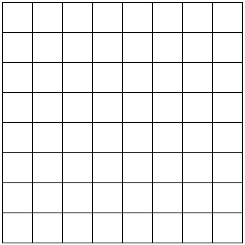
(a) Cartesian (QUAD) mesh

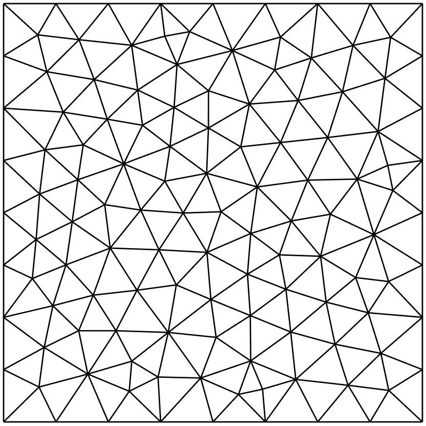
(b) Triangular (TRI) mesh

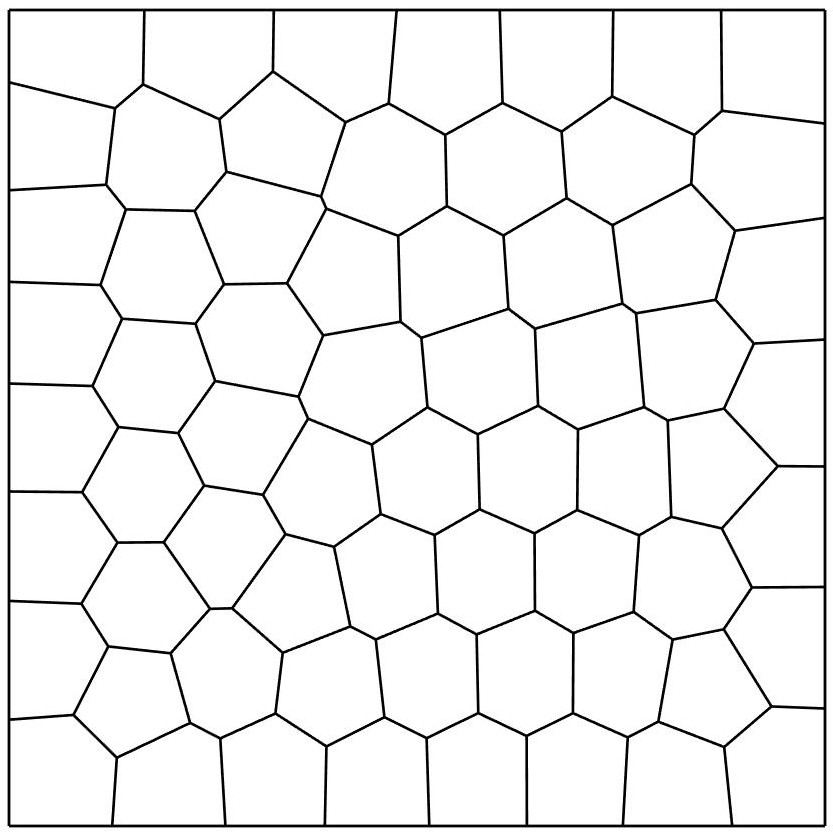
(c) CVT (CVT) mesh

Figure 1: Example of polygonal meshes used in the numerical tests.

mesh	$1/h$	# elements	# nodes	# DoFs
QUAD	128	16384	16641	49923
TRI	128	56932	28723	86169
CVT	128	16384	32943	98829

Table 1: Mesh size parameter $h$, number of elements, number of nodes and number of degrees of freedom (DoFs) of the polygonal meshes used in the numerical tests.

For the computational mesh, we consider three different mesh families, i.e., quadrilateral (QUAD), triangular (TRI) and central Voronoi tessellation (CVT) meshes. An example of a mesh of each family is shown in Figure 1. The corresponding number of elements, number of nodes, and number of degrees of freedom of the meshes used in all tests (except Test 4.1.1) are reported in Table 1.

Finally, the simulations have been performed using an in-house Fortran90 parallel code based on the PETSc library [11]. Except otherwise stated, the parallel tests were run on 32 cores of the INDACO linux cluster at the University of Milan (indaco.unimi.it).

4.1 Advective Cahn-Hilliard problem

We consider two scenarios: the evolution of a cross (Tests 1 and 2, Figure 2) and a spinoidal decomposition (Test 3, Figure 3). In both cases, the convective field $\mathbf{u}$ is taken from [58], i.e.

$$\mathbf{u}(x,y)=f(r)(2y-1,1-2x)^{T},\quad(x,y)\in\Omega=(0,1)^{2}$$

where

$$f(r)=\frac{1}{2}\left(1+\tanh\left(\beta\left(\frac{1}{2}-\epsilon-r\right)\right)\right)\quad\mbox{ and }\quad r=\sqrt{\left(x-\frac{1}{2}\right)^{2}+\left(y-\frac{1}{2}\right)^{2}},$$

with $\beta=200$ and $\epsilon=0.1$. The parameters Pe and $\gamma$ in system (1) are set to 100 and 0.01, respectively.

Advective Cahn-Hilliard problem, evolution of a cross
QUAD mesh with 147456 elements, DoFs = 444675
$p$	Mumps		BJ			GAMG			bAMG
	nit	$T_{sol}$	nit	it	$T_{sol}$	nit	it	$T_{sol}$	nit	it	$T_{sol}$
1	2.2	67.8	2.2	14.7	15.5	2.2	11.5	27.8	2.2	13.3	36.7
2	2.2	39.4	2.2	33.9	10.9	2.2	13.8	19.4	2.2	13.4	21.1
4	2.2	24.4	2.2	37.4	8.6	2.2	13.8	10.1	2.2	13.8	12.9
8	2.2	21.6	2.2	45.8	11.7	2.2	14.2	12.7	2.2	14.0	13.3
16	2.2	14.3	2.2	46.2	6.4	2.2	14.4	7.3	2.2	14.0	8.1
32	2.2	7.8	2.2	45.0	1.1	2.2	14.4	1.7	2.2	14.1	2.3
48	2.2	7.2	2.2	43.7	0.82	2.2	14.8	1.3	2.2	14.2	1.7
CVT mesh with 147456 elements, DoFs = 884814
$p$	Mumps		BJ			GAMG			bAMG
	nit	$T_{sol}$	nit	it	$T_{sol}$	nit	it	$T_{sol}$	nit	it	$T_{sol}$
1	OoM	OoM	2.2	32.2	44.9	2.2	18.9	88.7	2.2	21.1	135.7
2	2.2	202.1	2.2	79.6	36.1	2.2	25.6	67.8	2.2	24.1	172.2
4	2.2	123.9	2.2	95.9	27.6	2.2	28.5	59.8	2.2	25.6	125.3
8	2.2	85.4	2.2	107.4	23.9	2.2	30.4	45.9	2.2	26.9	74.6
16	2.2	53.2	2.2	110.6	14.6	2.2	30.7	39.6	2.2	27.2	38.1
32	2.2	32.4	2.2	109.7	4.7	2.2	31.2	34.3	2.2	27.1	18.1
48	2.2	27.2	2.2	108.3	3.2	2.2	30.8	30.5	2.2	27.2	12.9

Table 2: Strong scaling test on QUAD and CVT meshes, Advective Cahn-Hilliard, evolution of a cross. $p$=number of procs; nit=average Newton iterations per time step; it=average GMRES iterations per Newton iteration; $T_{sol}$=average CPU time in seconds per time step; OoM=out of memory.

4.1.1 Test 1: parallel performance of the solver

We first study the performance of the parallel solver by comparing four different methods:

• Mumps: the Jacobian system at each Newton iteration is solved by the parallel direct solver Mumps [4, 5];

• BJ: the Jacobian system at each Newton iteration is solved by the Block-Jacobi preconditioner implemented in the PETSc object PCBJACOBI;

• GAMG: the Jacobian system at each Newton iteration is solved by the Algebraic Multigrid preconditioner implemented in the PETSc object PCGAMG, with default settings;

• bAMG: the Jacobian system at each Newton iteration is solved by the Algebraic Multigrid preconditioner boomerAMG [54] of the HYPRE library [44].

The initial datum $c_{0}$ is a piecewise constant function whose jump set has the shape of a cross, see Figure 2, Panels (a-e-i). The time step size considered is $\tau=2e-5$ and the simulation is run for 50 time steps, up to $T=1e-3$. The unit square domain is discretized by a QUAD mesh of 147456 elements ($1/h=384$, DoFs = 444675) and a CVT mesh of 147456 elements ($1/h=384$, DoFs = 884814); see Table 2. We increase the number of processors from 1 to 48, keeping fixed the global number of DoFs, thus performing a strong scaling test. The code is run on the Galileo100 cluster of CINECA laboratory (www.cineca.it).

The results show that the four parallel solvers are all scalable, since the CPU times reduce when the number of processors increase. As expected, the Algebraic Multigrid preconditioners exhibit a scalable behavior of GMRES iterations, which remain almost constant with respect to the number of processors. The BJ preconditioner shows an initial increase in terms of iterations, but after 8-16 processors they remain stable. We believe that this scalable behavior of the BJ preconditioner is due to the dominant effect of the mass matrix, which improves the conditioning of the Jacobian linear system. Indeed, the most effective solver results to be the BJ preconditioner, which in case of the CVT mesh is about 9 times as fast as Mumps, 10 times as fast as GAMG and 4 times as fast as bAMG.

QUAD mesh

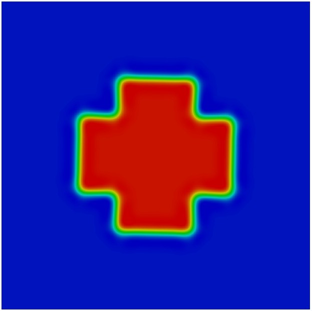
(a) $t=0.01$

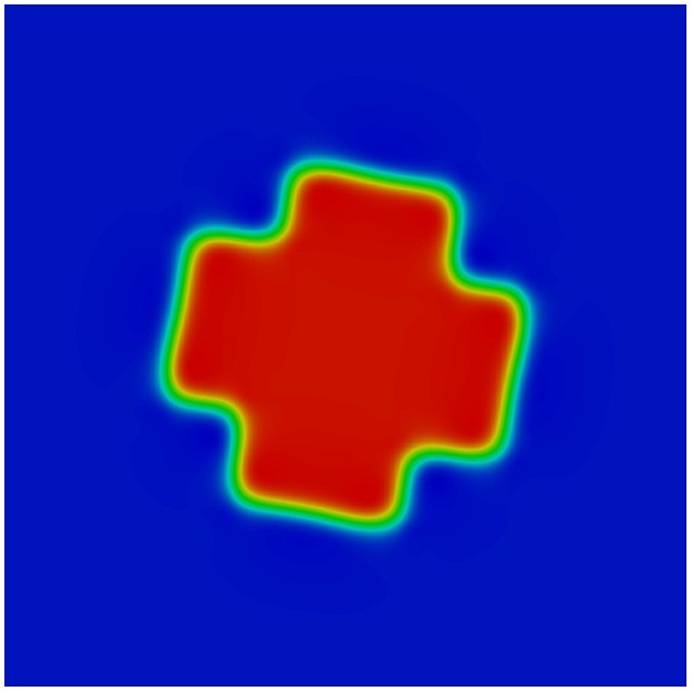
(b) t = 0.1

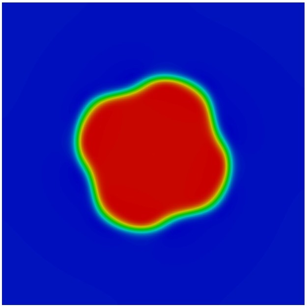
(c) $t=1$

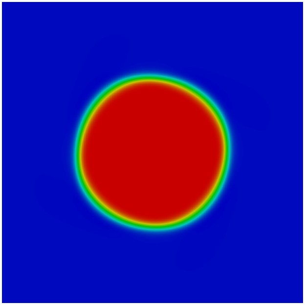
(d) $t=10$

TRI mesh

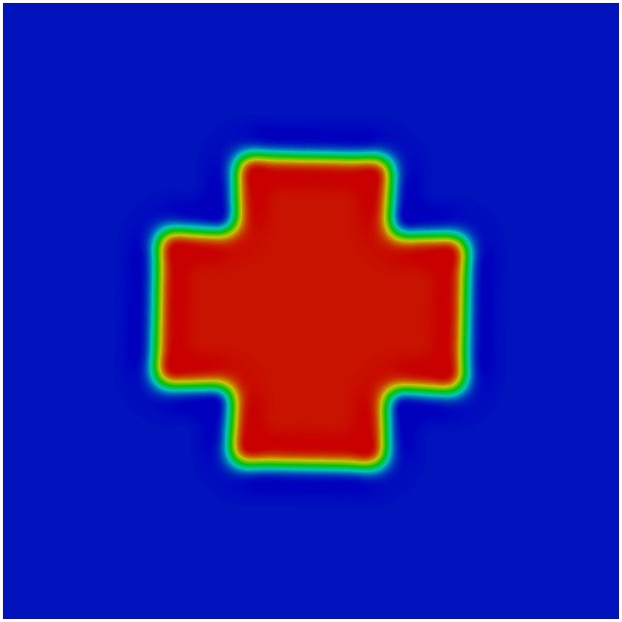
(e) $t=0.01$

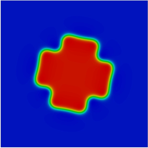
(f) t = 0.1

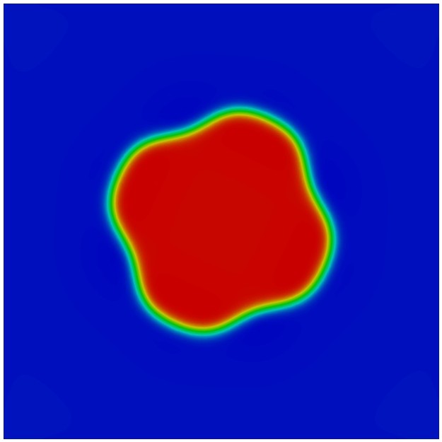
(g) $t=1$

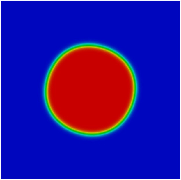
(h) $t=10$

CVT mesh

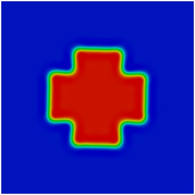
(i) $t=0.01$

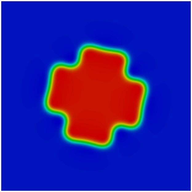
(j) t = 0.1

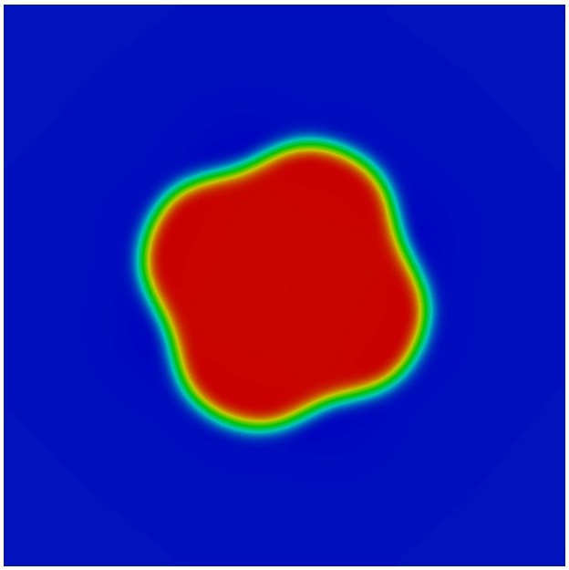
(k) $t=1$

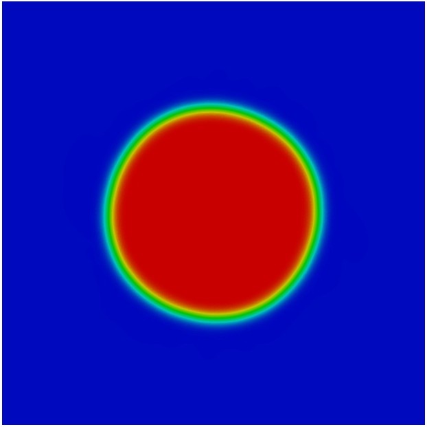
(l) $t=10$

Figure 2: Test 2, evolution of a cross with convection on the unit square, $\gamma=1/100$, $\text{Pe}=100$. The mesh parameters are reported in Table 1.

4.1.2 Test 2: evolution of a cross under convection

As in the previous test, the initial datum $c_{0}$ is again a piecewise constant function whose jump set has the shape of a cross. The time step size considered is $\tau=2e-5$ and the simulation is run for $500000$ time steps, up to $T=10$. The evolution of the cross simulated on the three computational meshes with data reported in Table 1 is displayed in Figure 2. The cross, rotating under the convective field, evolves towards a circle.

QUAD mesh

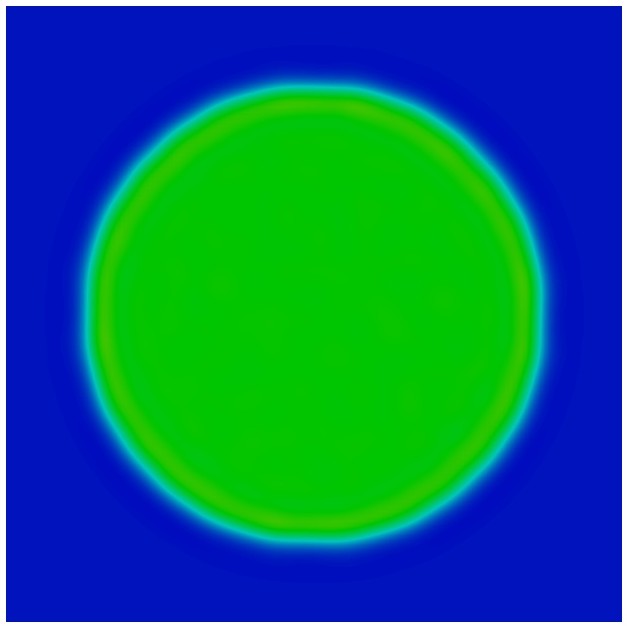
(a) $t=0.01$

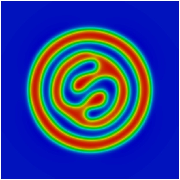
(b) $t=1$

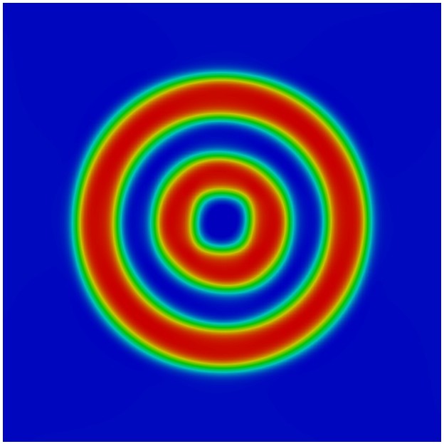
(c) $t=5$

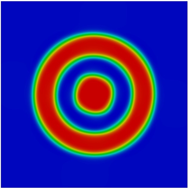
(d) $t=10$

TRI mesh

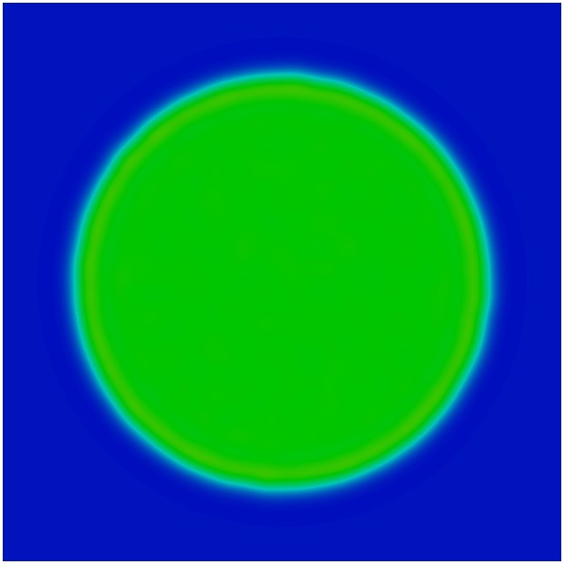
(e) $t=0.01$

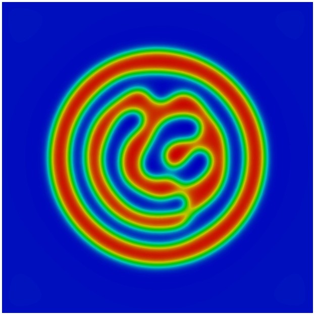
(f) $t=1$

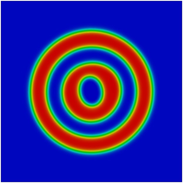
(g) $t=5$

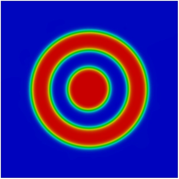
(h) $t=10$

CVT mesh

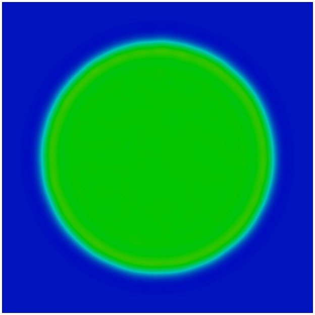
(i) $t=0.01$

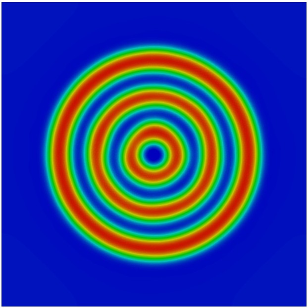
(j) $t=1$

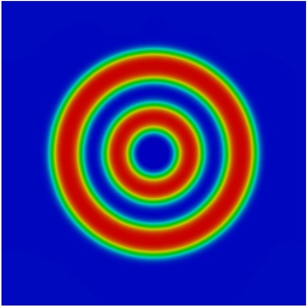
(k) $t=5$

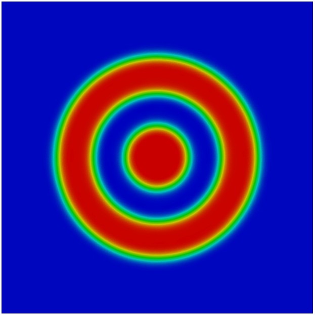
(l) $t=10$

Figure 3: Test 3, spinoidal decomposition of a random disk with convection on the unit square, $\gamma=1/100$, $\text{Pe}=100$. The mesh parameters are reported in Table 1.

4.1.3 Test 3: evolution of spinodal decomposition under convection

The initial datum is now a small uniformly distributed random perturbation about zero, within a circle; see Figure 3, Panels (a-e-i). The time step size considered is $\tau=2e-5$ and the simulation is run for $500000$ time steps, up to $T=10$. The evolution of the spinoidal decomposition on the three computational meshes is displayed in Figure 3. The initial random distribution evolves very quickly into bulk regions. Then, the convective term makes the bulk regions to form concentric circles, which tends very slowly to a central circular bulk region.

4.2 Cahn-Hilliard inpainting problem

We consider three scenarios: inpainting of a double stripe (Test 4, Figure 4), inpaiting of a cross (Test 5, Figure 5) and inpaiting of a circle (Test 6, Figure 6). The time step size considered is $\tau=2e-5$ and the simulation is run for 50 time steps, up to $T=1e-3$. The parameters $\gamma$ and $\lambda_{0}$ are set to 0.01 and 50000, respectively. In all next tests, the time step size considered is $\tau=2e-5$ and the simulation is run for $1000$ time steps, up to $T=0.02$.

QUAD mesh

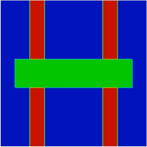
(a) $t=0$

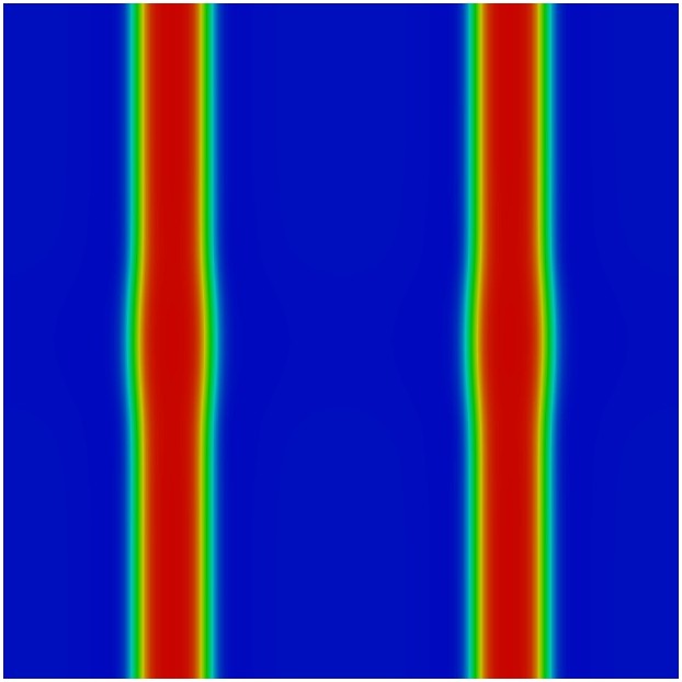
(b) $t=0.02$

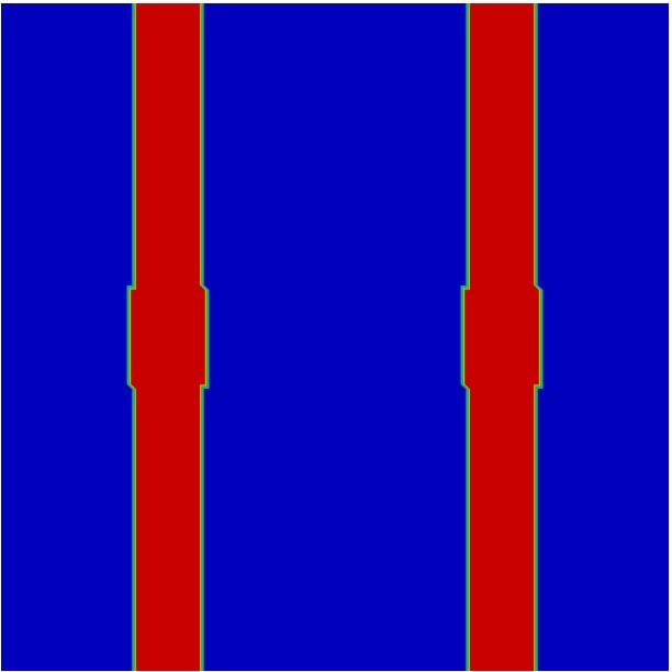
(c) $t=0.02$(binary)

TRI mesh

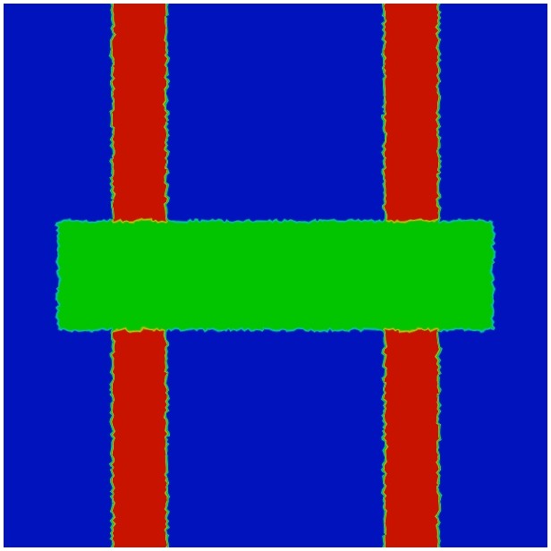
(d) $t=0$

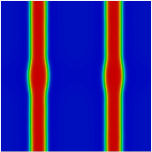
(e) $t=0.02$

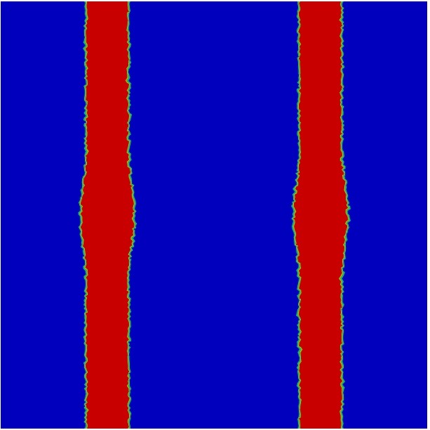
(f) $t=0.02$(binary)

CVT mesh

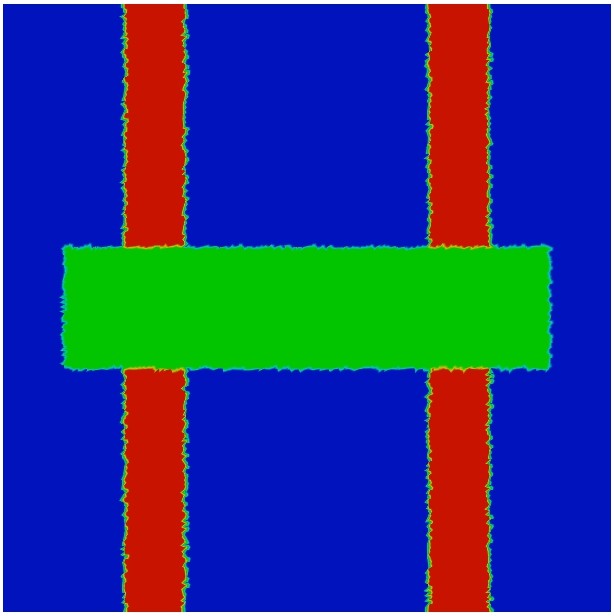
(g) $t=0$

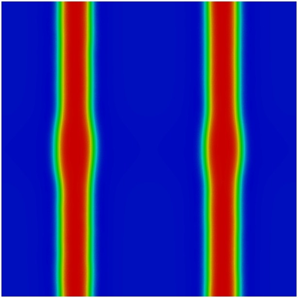
(h) $t=0.02$

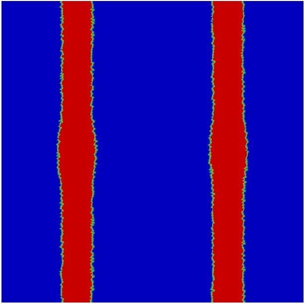
(i) $t=0.02$(binary)

Figure 4: Test 4, impainting of a double stripe. The mesh parameters are reported in Table 1. Left: initial configuration ($t=0$). Middle: final configuration ($t=T=0.02$). Right: final configuration ($t=T=0.02$) without smoothing effects, projecting the solution $c$ to 0.95 if $c>0$ and to $-0.95$ if $c<0$.

4.2.1 Test 4: inpainting of a double stripe

In this test, the initial configuration consists of two vertical stripes with a central horizontal damage, see Figure 4. At the final instant $t=T=0.02$, the correct double stripe configuration is recovered, for all mesh configurations. We show also the final configuration without smoothing effects, projecting the solution $c$ to 0.95 if $c>0$ and to $-0.95$ if $c<0$ (binary).

QUAD mesh

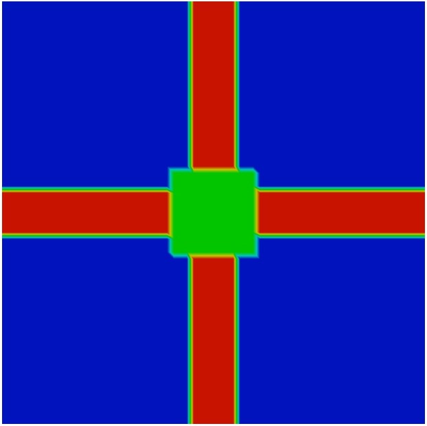
(a) $t=0$

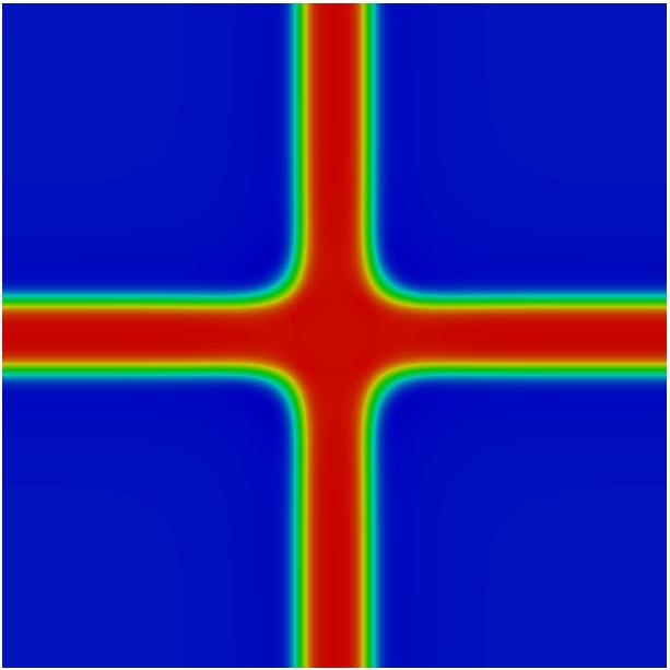
(b) $t=0.02$

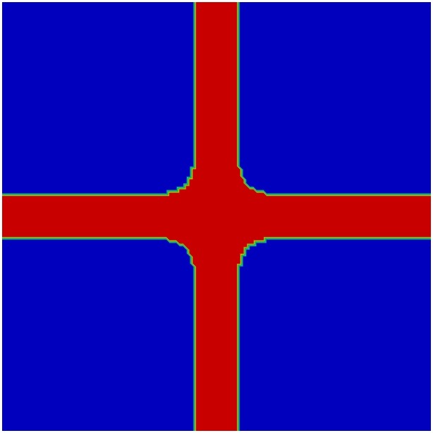
(c) $t=0.02$(binary)

TRI mesh

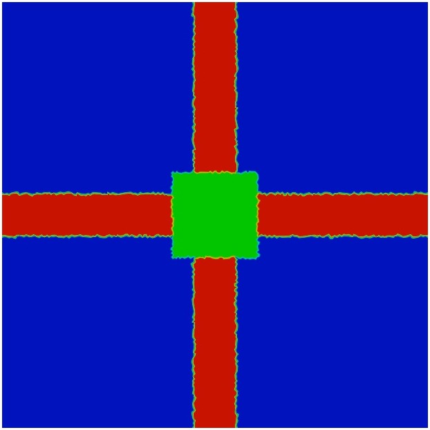
(d) $t=0$

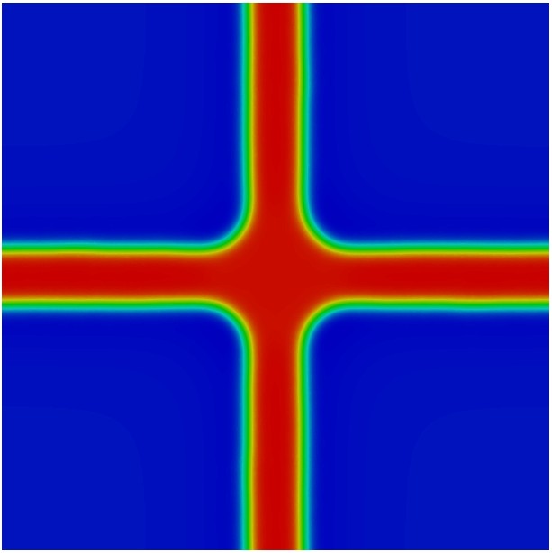
(e) $t=0.02$

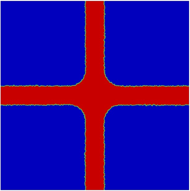
(f) $t=0.02$(binary)

CVT mesh

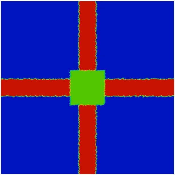
(g) $t=0$

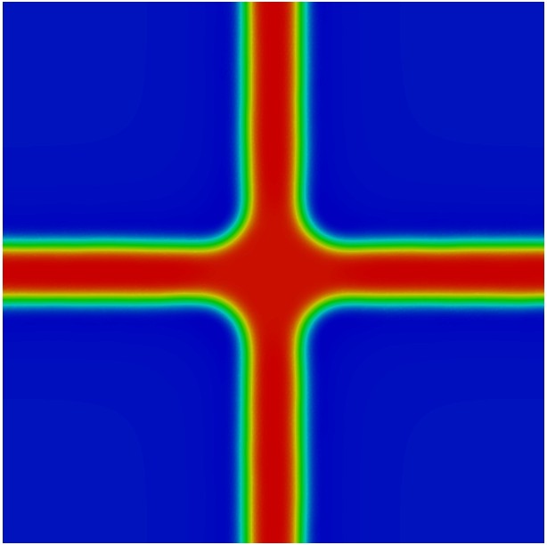
(h) $t=0.02$

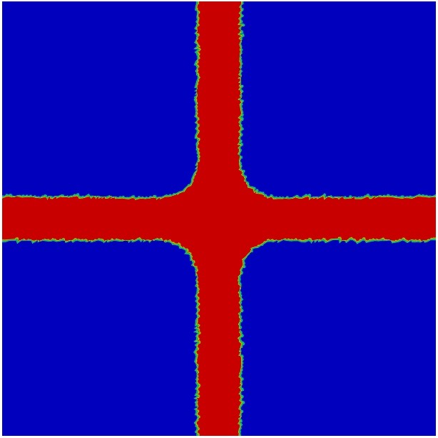
(i) $t=0.02$(binary)

Figure 5: Test 5, impainting of a cross. The mesh parameters are reported in Table 1. Left: initial configuration ($t=0$). Middle: final configuration ($t=T=0.02$). Right: final configuration ($t=T=0.02$) without smoothing effects, projecting the solution $c$ to 0.95 if $c>0$ and to $-0.95$ if $c<0$.

4.2.2 Test 5: inpainting of a cross

Here, the initial configuration consists of two stripes, one vertical and one horizontal, crossing at the center of the domain, with a central square damage, see Figure 5. At the final instant $T=0.02$, the correct cross configuration is recovered. As before, we also report the final configuration without smoothing effects, projecting the solution $c$ to 0.95 if $c>0$ and to $-0.95$ if $c<0$ (binary).

QUAD mesh

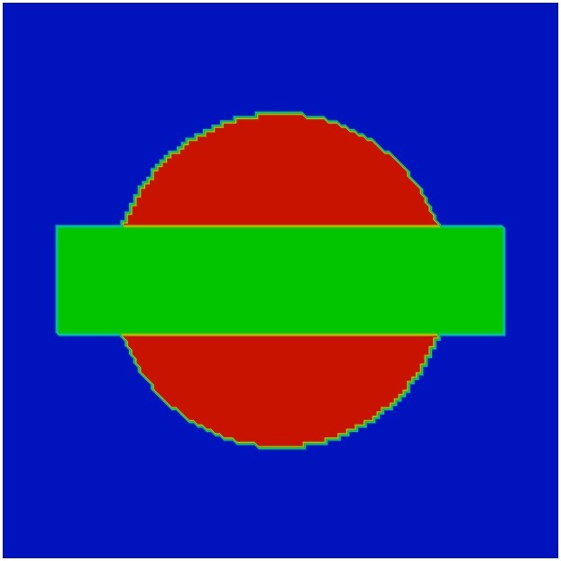
(a) $t=0$

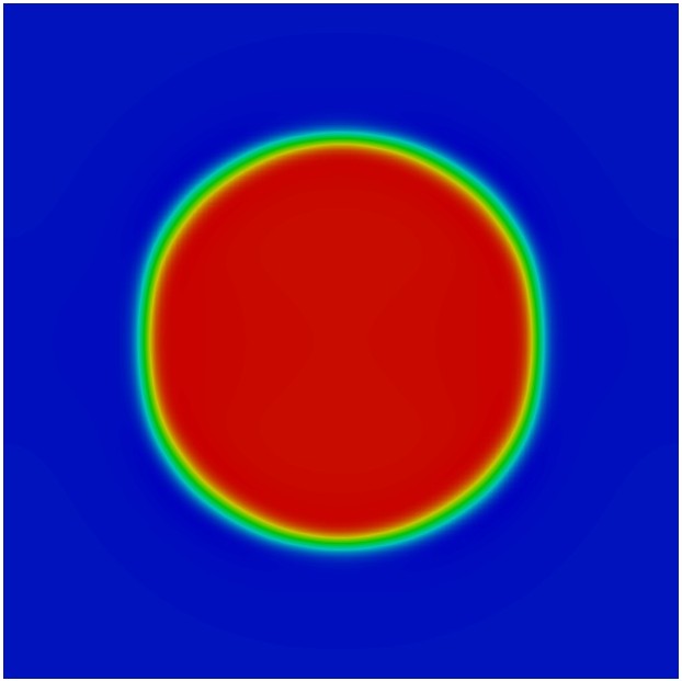
(b) $t=0.02$

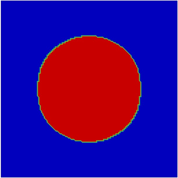
(c) $t=0.02$ (binary)

TRI mesh

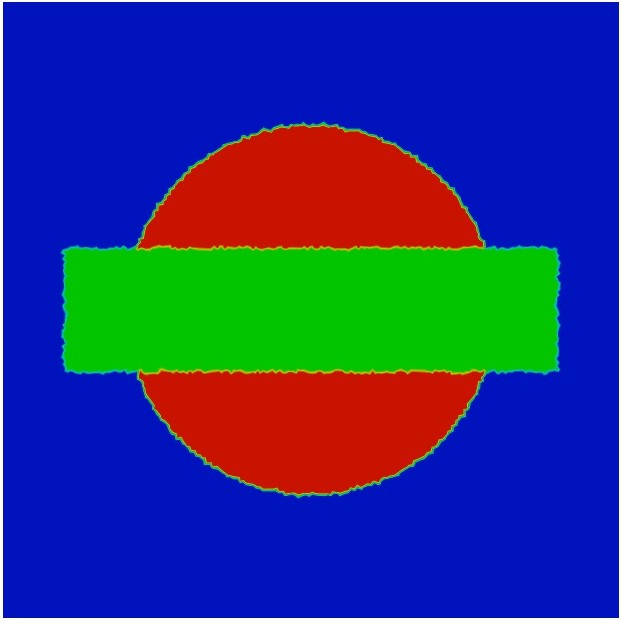
(d) $t=0$

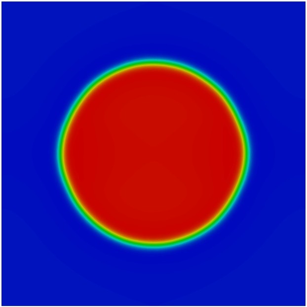
(e) $t=0.02$

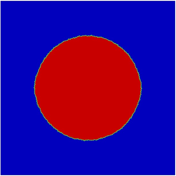
(f) $t=0.02$(binary)

CVT mesh

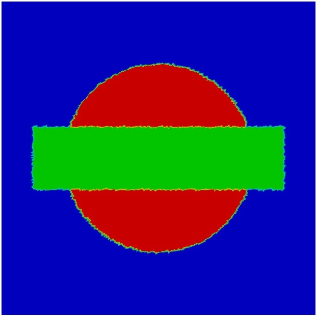
(g) $t=0$

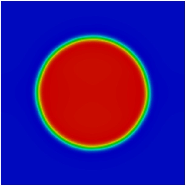
(h) $t=0.02$

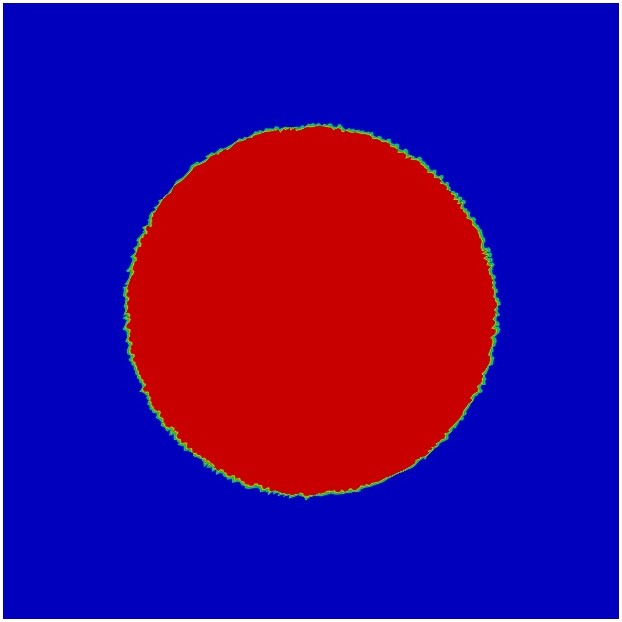
(i) $t=0.02$(binary)

Figure 6: Test 6, impainting of a circle. The mesh parameters are reported in Table 1. Left: initial configuration ($t=0$). Middle: final configuration ($t=T=0.02$). Right: final configuration ($t=T=0.02$) without smoothing effects, projecting the solution $c$ to 0.95 if $c>0$ and to $-0.95$ if $c<0$.

4.2.3 Test 6: inpainting of a circle

In the final test, the initial configuration is a circle with a horizontal central damage, see Figure 6. At the final instant $T=0.02$, the correct circle configuration is recovered, for all mesh configurations. This can be appreciated also from Figure 6 (right panel) where we report the final configuration (binary plot) projecting the solution $c$ to 0.95 if $c>0$ and to $-0.95$ if $c<0$.

5 Conclusions

In this paper we considered the $C^{1}$-Virtual Element conforming approximation on polygonal meshes of some variants of the Cahn-Hilliard equation. In particular, we focused on the advective Cahn-Hilliard problem and the Cahn-Hilliard impainting problem. In the first part of the paper we introduced the continuous problems and we gave a detailed description of the virtual element discretizations, while in the second part we numerically explored the efficacy of the proposed methodology through a wide campaign of numerical experiments.

References

- [1] R. A. Adams. Sobolev spaces, volume 65 of Pure and Applied Mathematics. Academic Press, New York-London, 1975.
- [2] A. Agosti, P.F. Antonietti, P. Ciarletta, M. Grasselli, and M. Verani. A Cahn-Hilliard–type equation with application to tumor growth dynamics. Mathematical Methods in the Applied Sciences, 40(18):7598–7626, 2017.
- [3] B. Ahmad, A. Alsaedi, F. Brezzi, L. D. Marini, and A. Russo. Equivalent projectors for virtual element methods. Comput. Math. Appl., 66(3):376–391, 2013.
- [4] P. R. Amestoy, I. S. Duff, J.-Y. L’Excellent, and J. Koster. A fully asynchronous multifrontal solver using distributed dynamic scheduling. SIAM J. Matr. Anal. Appl., 23(1):15–41, 2001.
- [5] P. R. Amestoy, A. Guermouche, J.-Y. L’Excellent, and S. Pralet. Hybrid scheduling for the parallel solution of linear systems. Paral. Comput., 32(2):136–156, 2006.
- [6] P. F. Antonietti, L. Beirão da Veiga, S. Scacchi, and M. Verani. A virtual element method for the Cahn-Hilliard equation with polygonal meshes. SIAM J. Numer. Anal., 54(1):34–56, 2016.
- [7] P. F. Antonietti, G. Manzini, S. Scacchi, and M. Verani. A review on arbitrarily regular virtuale element methods for elliptic partial differential equations. Math. Models Methods Appl. Sci., 2021. in press.
- [8] P. F. Antonietti, G. Manzini, and M. Verani. The conforming virtual element method for polyharmonic problems. Comput. Math. Appl., 79(7):2021–2034, 2020.
- [9] J. H. Argyris, I. Fried, and D. W. Scharpf. The TUBA family of plate elements for the matrix displacement method. Aeronaut. J. R. Aeronaut. Soc., 72:701–709, 1968.
- [10] A.C. Aristotelous, O. Karakashian, and S.M. Wise. A mixed discontinuous galerkin, convex splitting scheme for a modified Cahn-Hilliard equation and an efficient nonlinear multigrid solver. Discrete and Continuous Dynamical Systems - Series B, 18(9):2211–2238, 2013.
- [11] S. Balay, S. Abhyankar, M. F. Adams, J. Brown, P. Brune, K. Buschelman, L. Dalcin, V. Eijkhout, W. D. Gropp, D. Kaushik, M. G. Knepley, D. A. May, L. C. McInnes, R. T. Mills, T. Munson, K. Rupp, P. Sanan, B. F. Smith, S. Zampini, H. Zhang, and H. Zhang. PETSc users manual. Technical Report ANL-95/11 - Revision 3.14, Argonne National Laboratory, 2020.
- [12] K. Bao, Y. Shi, S. Sun, and X.-P. Wang. A finite element method for the numerical solution of the coupled Cahn-Hilliard and navier-stokes system for moving contact line problems. Journal of Computational Physics, 231(24):8083–8099, 2012.
- [13] L. Beirão da Veiga, F. Brezzi, A. Cangiani, G. Manzini, L. D. Marini, and A. Russo. Basic principles of virtual element methods. Math. Models Methods Appl. Sci., 23(1):199–214, 2013.
- [14] L. Beirão da Veiga, F. Dassi, and A. Russo. High-order virtual element method on polyhedral meshes. Comput. Math. Appl., 74(5):1110–1122, 2017.
- [15] L. Beirão da Veiga, F. Dassi, and A. Russo. A virtual element method on polyhedral meshes. Comput. Math. Appl., 79(7):1936–1955, 2020.
- [16] L. Beirão da Veiga and G. Manzini. A virtual element method with arbitrary regularity. IMA J. Numer. Anal., 34(2):782–799, 2014.
- [17] L. Beirão da Veiga and G. Manzini. Residual a posteriori error estimation for the virtual element method for elliptic problems. ESAIM Math. Model. Numer. Anal., 49(2):577–599, 2015.
- [18] L. Beirão da Veiga, F. Brezzi, A. Cangiani, G. Manzini, L. D. Marini, and A. Russo. Basic principles of virtual element methods. Math. Models Methods Appl. Sci., 23(1):199–214, 2013.
- [19] L. Beirão da Veiga, F. Brezzi, L. D. Marini, and A. Russo. The Hitchhiker’s Guide to the Virtual Element Method. Math. Models Methods Appl. Sci., 24(8):1541–1573, 2014.
- [20] L. Beirão da Veiga, C. Lovadina, and A. Russo. Stability analysis for the virtual element method. Math. Mod.and Meth. in Appl. Sci., 27(13):2557–2594, 2017.
- [21] K. Bell. A refined triangular plate bending finite element. Int. J. Numer. Meth. Eng., 1(1):101–122, 1969. cited By 156.
- [22] A. Bertozzi, S. Esedoǧlu, and A. Gillette. Analysis of a two-scale Cahn-Hilliard model for binary image inpainting. Multiscale Modeling and Simulation, 6(3):913–936, 2007.
- [23] A.L. Bertozzi, S. Esedoglu, and A. Gillette. Inpainting of binary images using the Cahn-Hilliard equation. IEEE Transactions on Image Processing, 16(1):285–291, 2007.
- [24] M.J. Borden, C.V. Verhoosel, M.A. Scott, T.J.R. Hughes, and C.M. Landis. A phase-field description of dynamic brittle fracture. Computer Methods in Applied Mechanics and Engineering, 217-220:77–95, 2012.
- [25] S. C. Brenner, Q. Guan, and L. Y. Sung. Some estimates for virtual element methods. Comput. Methods Appl. Math., 17(4):553–574, 2017.
- [26] S. C. Brenner and L.-Y. Sung. Virtual enriching operators. Calcolo, 56(4):1–25, 2019.
- [27] S. C. Brenner and L.Y. Sung. Virtual element methods on meshes with small edges or faces. Math. Models Methods Appl. Sci., 28(7):1291–1336, 2018.
- [28] F. Brezzi and L. D. Marini. Virtual element method for plate bending problems. Comput. Methods Appl. Mech. Engrg., 253:455–462, 2013.
- [29] F. Brezzi and L. D. Marini. Virtual element methods for plate bending problems. Comput. Methods Appl. Mech. Engrg., 253:455–462, 2013.
- [30] J. W. Cahn and J. E. Hilliard. Free energy of a nonuniform system. I. Interfacial free energy. The Journal of Chemical Physics, 28:258–0, 1958.
- [31] C. Chatelain, T. Balois, P. Ciarletta, and M. Ben Amar. Emergence of microstructural patterns in skin cancer: A phase separation analysis in a binary mixture. New Journal of Physics, 13, 2011.
- [32] F. Chave, D.A. Di Pietro, F. Marche, and F. Pigeonneaux. A hybrid high-order method for the Cahn-Hilliard problem in mixed form. SIAM Journal on Numerical Analysis, 54(3):1873–1898, 2016.
- [33] L.-Q. Chen. Phase-field models for microstructure evolution. Annual Review of Materials Science, 32:113–140, 2002.
- [34] C. Chinosi and L. D. Marini. Virtual element method for fourth order problems: -estimates. Comput. Math. Appl., 72(8):1959–1967, 2016.
- [35] R. W. Clough and J. L. Tocher, editors. Finite element stiffness matrices for analysis of plates in bending. Proceedings of the Conference on Matrix Methods in Structural Mechanics, 1965.
- [36] F. Della Porta and M. Grasselli. Convective nonlocal Cahn-Hilliard equations with reaction terms. Discrete and Continuous Dynamical Systems - Series B, 20(5):1529–1553, 2015.
- [37] K.R. Elder, M. Katakowski, M. Haataja, and M. Grant. Modeling elasticity in crystal growth. Physical Review Letters, 88(24):2457011–2457014, 2002.
- [38] C. M. Elliott and D. A. French. A nonconforming finite-element method for the two-dimensional Cahn-Hilliard equation. SIAM J. Numer. Anal., 26(4):884–903, 1989.
- [39] C.M. Elliott and D.A. French. Numerical studies of the Cahn-Hilliard equation for phase separation. IMA Journal of Applied Mathematics (Institute of Mathematics and Its Applications), 38(2):97–128, 1987.
- [40] C.M. Elliott and Z. Songmu. On the Cahn-Hilliard equation. Archive for Rational Mechanics and Analysis, 96(4):339–357, 1986.
- [41] H. Emmerich. Advances of and by phase-field modelling in condensed-matter physics. Advances in Physics, 57(1):1–87, 2008.
- [42] H. Emmerich, L. Gránásy, and H. Löwen. Selected issues of phase-field crystal simulations. European Physical Journal Plus, 126(10):1–18, 2011.
- [43] G. Engel, K. Garikipati, T.J.R. Hughes, M.G. Larson, L. Mazzei, and R.L. Taylor. Continuous/discontinuous finite element approximations of fourth-order elliptic problems in structural and continuum mechanics with applications to thin beams and plates, and strain gradient elasticity. Computer Methods in Applied Mechanics and Engineering, 191(34):3669–3750, 2002.
- [44] R. D. Falgout and U. M. Yang. hypre: A library of high performance preconditioners. In P. M. A. Sloot, A. G. Hoekstra, C. J. K. Tan, and J. J. Dongarra, editors, Computational Science — ICCS 2002, pages 632–641, Berlin, Heidelberg, 2002. Springer Berlin Heidelberg.
- [45] X. Feng. Fully discrete finite element approximations of the navier-stokes-cahn- hilliard diffuse interface model for two-phase fluid flows. SIAM Journal on Numerical Analysis, 44(3):1049–1072, 2006.
- [46] X. Feng and A. Prohl. Error analysis of a mixed finite element method for the Cahn-Hilliard equation. Numerische Mathematik, 99(1):47–84, 2004.
- [47] F. Frank, C. Liu, A. Scanziani, F.O. Alpak, and B. Riviere. An energy-based equilibrium contact angle boundary condition on jagged surfaces for phase-field methods. Journal of Colloid and Interface Science, 523:282–291, 2018.
- [48] S. Frigeri, M. Grasselli, and E. Rocca. On a diffuse interface model of tumour growth. European Journal of Applied Mathematics, 26(2):215–243, 2015.
- [49] C.G. Gal and M. Grasselli. Asymptotic behavior of a Cahn-Hilliard-navier-stokes system in 2d. Annales de l’Institut Henri Poincare (C) Analyse Non Lineaire, 27(1):401–436, 2010.
- [50] C.G. Gal, M. Grasselli, and A. Miranville. Cahn–hilliard–navier–stokes systems with moving contact lines. Calculus of Variations and Partial Differential Equations, 55(3), 2016.
- [51] M. Grasselli and M. Pierre. Energy stable and convergent finite element schemes for the modified phase field crystal equation. ESAIM: Mathematical Modelling and Numerical Analysis, 50(5):1523–1560, 2016.
- [52] H. Gómez, V.M. Calo, Y. Bazilevs, and T.J.R. Hughes. Isogeometric analysis of the Cahn-Hilliard phase-field model. Computer Methods in Applied Mechanics and Engineering, 197(49-50):4333–4352, 2008.
- [53] A. Hawkins-Daarud, K.G. van der Zee, and J. Tinsley Oden. Numerical simulation of a thermodynamically consistent four-species tumor growth model. International Journal for Numerical Methods in Biomedical Engineering, 28(1):3–24, 2012.
- [54] V. E. Henson and U. M. Yang. BoomerAMG: A parallel algebraic multigrid solver and preconditioner. Appl. Numer. Math., 41:155–177, 2002.
- [55] J. Hu, T. Lin, and Q. Wu. A construction of conforming finite element spaces in any dimension, 2021. arXiv:2103.14924.
- [56] J. Hu and S. Zhang. The minimal conforming finite element spaces on rectangular grids. Math. Comp., 84(292):563–579, 2015.
- [57] X. Huang. -conforming virtual elements in arbitrary dimension, 2021. arXiv:2105.12973.
- [58] D. Kay, V. Styles, and E. Süli. Discontinuous Galerkin finite element approximation of the Cahn-Hilliard equation with convection. SIAM J. Numer. Anal., 47(4):2660–2685, 2009.
- [59] D. Kay, V. Styles, and R. Welford. Finite element approximation of a Cahn-Hilliard-Navier-Stokes system. Interfaces and Free Boundaries, 10(1):15–43, 2008.
- [60] C. Kuhn and R. Müller. A continuum phase field model for fracture. Engineering Fracture Mechanics, 77(18):3625–3634, 2010.
- [61] M. Li, J. Zhao, C. Huang, and S. Chen. Conforming and nonconforming vems for the fourth-order reaction–subdiffusion equation: a unified framework. IMA J. Numer. Anal., 2021.
- [62] C. Liu, F. Frank, and B.M. Rivière. Numerical error analysis for nonsymmetric interior penalty discontinuous galerkin method of cahn–hilliard equation. Numerical Methods for Partial Differential Equations, 35(4):1509–1537, 2019.
- [63] Ju Liu, Luca Dedè, John A. Evans, Micheal J. Borden, and Thomas J. R. Hughes. Isogeometric analysis of the advective Cahn-Hilliard equation: spinodal decomposition under shear flow. J. Comput. Phys., 242:321–350, 2013.
- [64] X. Liu, Z. He, and Z. Chen. A fully discrete virtual element scheme for the cahn–hilliard equation in mixed form. Computer Physics Communications, 246, 2020.
- [65] Carlo Lovadina, David Mora, and Iván Velásquez. A virtual element method for the von Kármán equations. ESAIM Math. Model. Numer. Anal., 55(2):533–560, 2021.
- [66] C. Miehe, F. Welschinger, and M. Hofacker. Thermodynamically consistent phase-field models of fracture: Variational principles and multi-field fe implementations. International Journal for Numerical Methods in Engineering, 83(10):1273–1311, 2010.
- [67] Alain Miranville. The Cahn-Hilliard equation, volume 95 of CBMS-NSF Regional Conference Series in Applied Mathematics. Society for Industrial and Applied Mathematics (SIAM), Philadelphia, PA, 2019. Recent advances and applications.
- [68] N. Moelans, B. Blanpain, and P. Wollants. An introduction to phase-field modeling of microstructure evolution. Calphad: Computer Coupling of Phase Diagrams and Thermochemistry, 32(2):268–294, 2008.
- [69] D. Mora, G. Rivera, and I. Velásquez. A virtual element method for the vibration problem of Kirchhoff plates. ESAIM Math. Model. Numer. Anal., 52(4):1437–1456, 2018.
- [70] D. Mora and A. Silgado. A virtual element method for the stationary quasi-geostrophic equations of the ocean. Comput. Math. Appl., 2021.
- [71] D. Mora and I. Velásquez. A virtual element method for the transmission eigenvalue problem. Math. Models Methods Appl. Sci., 28(14):2803–2831, 2018.
- [72] D. Mora and I. Velásquez. Virtual element for the buckling problem of Kirchhoff-Love plates. Comput. Methods Appl. Mech. Engrg., 360:112687, 22, 2020.
- [73] F. Regazzoni, N. Parolini, and M. Verani. Topology optimization of multiple anisotropic materials, with application to self-assembling diblock copolymers. Computer Methods in Applied Mechanics and Engineering, 338:562–596, 2018.
- [74] I. Steinbach. Phase-field models in materials science. Modelling and Simulation in Materials Science and Engineering, 17(7), 2009.
- [75] E.L. Thomas, D.M. Anderson, C.S. Henkee, and D. Hoffman. Periodic area-minimizing surfaces in block copolymers. Nature, 334(6183):598–601, 1988.
- [76] C. Wang and S.M. Wise. An energy stable and convergent finite-difference scheme for the modified phase field crystal equation. SIAM Journal on Numerical Analysis, 49(3):945–969, 2011.
- [77] G.N. Wells, E. Kuhl, and K. Garikipati. A discontinuous galerkin method for the Cahn-Hilliard equation. Journal of Computational Physics, 218(2):860–877, 2006.
- [78] S.M. Wise, J.S. Lowengrub, H.B. Frieboes, and V. Cristini. Three-dimensional multispecies nonlinear tumor growth-i. model and numerical method. Journal of Theoretical Biology, 253(3):524–543, 2008.
- [79] S. Zhang. A family of 3D continuously differentiable finite elements on tetrahedral grids. Appl. Numer. Math., 59(1):219–233, 2009.
- [80] S. Zhang. A family of differentiable finite elements on simplicial grids in four space dimensions. Math. Numer. Sin., 38(3):309–324, 2016.