A Theoretical Understanding of Gradient Bias in Meta-Reinforcement Learning

Abstract

Gradient-based Meta-RL (GMRL) refers to methods that maintain two-level optimisation procedures wherein the outer-loop meta-learner guides the inner-loop gradient-based reinforcement learner to achieve fast adaptations. In this paper, we develop a unified framework that describes variations of GMRL algorithms and points out that existing stochastic meta-gradient estimators adopted by GMRL are actually biased. Such meta-gradient bias comes from two sources: 1) the compositional bias incurred by the two-level problem structure, which has an upper bound of $\mathcal{O}\big{(}K\alpha^{K}\hat{\sigma}_{\text{In}}|\tau|^{-0.5}\big{)}$ w.r.t. inner-loop update step $K$, learning rate $\alpha$, estimate variance $\hat{\sigma}^{2}_{\text{In}}$ and sample size $|\tau|$, and 2) the multi-step Hessian estimation bias $\hat{\Delta}_{H}$ due to the use of autodiff, which has a polynomial impact $\mathcal{O}\big{(}(K-1)(\hat{\Delta}_{H})^{K-1}\big{)}$ on the meta-gradient bias. We study tabular MDPs empirically and offer quantitative evidence that testifies our theoretical findings on existing stochastic meta-gradient estimators. Furthermore, we conduct experiments on Iterated Prisoner’s Dilemma and Atari games to show how other methods such as off-policy learning and low-bias estimator can help fix the gradient bias for GMRL algorithms in general.

1 Introduction

Meta Learning, also known as learning to learn, is proposed to equip intelligent agents with meta knowledge for fast adaptations [30]. Meta-Reinforcement Learning (RL) algorithms aim to train RL agents that can adapt to new tasks with only few examples [5, 10, 16]. For example, MAML-RL [10], a typical Meta-RL algorithm, learns the initial parameters of an agent’s policy so that the agent can rapidly adapt to new environments with a limited number of policy-gradient updates. Recently, Meta-RL algorithms have been further developed beyond the scope of learning fast adaptations. An important direction is to conduct online meta-gradient learning for adaptively tuning algorithmic hyper-parameters [39, 41] or designing intrinsic reward [42] during training in one single task. Besides, there are Meta-RL developments that manage to discover new RL algorithms by learning algorithmic components or other fundamental concepts in RL, such as the policy gradient objective [26] or the TD-target [40], which can generalise to solve a distribution of different tasks.

In general, gradient-based Meta-RL (GMRL) tasks can be formulated by a two-level optimisation procedure. This procedure optimises the parameters of an outer-loop meta-learner, whose objective is dependent on a $K$-step policy update process (e.g., stochastic gradient descent) conducted by an inner-loop learner. Formally, this procedure can be written as:

$$\max_{\boldsymbol{\phi}}J^{K}(\boldsymbol{\phi}):=J^{\text{Out}}(\boldsymbol{\phi},\boldsymbol{\theta}^{K}),$$ (1)

         s.t. $$\boldsymbol{\theta}^{i+1}=\boldsymbol{\theta}^{i}+\alpha\nabla_{\boldsymbol{\theta}^{i}}J^{\text{In}}(\boldsymbol{\phi},\boldsymbol{\theta}^{i}),i\in\{0,1\ldots K-1\},$$

where $\boldsymbol{\theta}$ are inner-loop policy parameters, $\boldsymbol{\phi}$ are meta parameters, $\alpha$ is the learning rate, $J^{\text{In}}$ and $J^{\text{Out}}$ are value functions for the inner and the outer-loop learner. In solving Eq. (1), estimating the meta-gradient of $\nabla_{\boldsymbol{\phi}}J^{K}(\boldsymbol{\phi})$ from a two-level optimisation process is non-trivial; how to conduct accurate estimation on $\nabla_{\boldsymbol{\phi}}J^{K}(\boldsymbol{\phi})$ has been a critical yet challenging research problem [23, 29, 33].

In this paper, we point out that the meta-gradient estimators adopted by many recent GMRL methods [26, 40] are in fact biased. We conclude that such bias comes from two sources: (1) the compositional bias and (2) the multi-step Hessian bias. The compositional bias origins from the discrepancy between the sampled policy gradient $\nabla_{\boldsymbol{\theta}}\hat{J}^{\text{In}}$ and expected policy gradient $\nabla_{\boldsymbol{\theta}}J^{\text{In}}$, and the multi-step Hessian estimation bias occurs due to the biased Hessian estimation $\nabla_{\boldsymbol{\theta}}^{2}\hat{J}^{\text{In}}$ resulting from the employment of automatic differentiation in modern GMRL implementations.

There are very few prior work that investigates the bias in GMRL, most of them limited to the Hessian estimation bias in the MAML-RL setting [29, 33]. Our paper investigates the above two biases in a broader setting and applies on generic meta-gradient estimators. For the compositional bias term, we offer the first theoretical analysis on its quantity, based on which we then investigate current mitigation solutions. For the multi-step Hessian bias, we provide rigorous analysis in GMRL settings particularly for those GMRL tasks where complex inner-loop optimisations are involved.

For the rest of the paper, we first introduce a unified Meta-RL framework that can describe variations of existing GMRL algorithms. Building on this framework, we offer two theoretical results that 1) the compositional bias has an upper bound of $\mathcal{O}\big{(}K\alpha^{K}\hat{\sigma}_{\text{In}}|\tau|^{-0.5}\big{)}$ with respect to the inner-loop update step $K$, the learning rate $\alpha$, the estimate variance $\hat{\sigma}^{2}_{\text{In}}$ and the sample size $|\tau|$, and 2) the multi-step Hessian bias $\hat{\Delta}_{H}$ has a polynomial impact of $\mathcal{O}\big{(}(K-1)(\hat{\Delta}_{H})^{K-1}\big{)}$. To validate our theoretical insights on these two biases, we conduct a comprehensive list ablation studies. Experiments over tabular MDP with MAML-RL [10] and LIRPG [42] demonstrate how quantitatively these two biases influence the estimation accuracy, which consolidates our theories.

Furthermore, our theoretical results help understand to what extent existing methods can mitigate theses two bias empirically. For the compositional bias, we show that off-policy learning methods can reduce the inner-loop policy gradient variance and the resulting compositional bias. For the multi-step Hessian bias, we study how the low-variance curvature technique based on Rothfuss et al. [29] can help correct the Hessian bias for general GMRL problems. We test these solutions on environments including iterated Prisoner’s Dilemma with off-policy corrected LOLA-DiCE [13], and eight Atari games based on MGRL [39] with the multi-step Hessian correction technique. Experimental results confirm that those bias-correction methods can substantially decrease the meta-gradients bias and improve the overall performance on rewards.

2 Related Work

A pioneering work that studies meta-gradient estimation is Al-Shedivat et al. [1] who discussed the biased estimation problem of MAML and proposed the E-MAML sample based formulation to fix the meta-gradient bias. Following work includes Rothfuss et al. [29], Liu et al. [23], Tang et al. [33] that tried to fix the meta-gradient estimation error by reducing the estimation variance so as to improve the performance. Moreover, Foerster et al. [12], Farquhar et al. [8], Mao et al. [24] discussed the higher-order gradient estimation in RL. Recently, Bonnet et al. [4], Vuorio et al. [36] proposed algorithms to balance the bias-variance trade-off for meta-gradient estimates. Within theoretical context of GMRL, most theoretical analysis focuses on convergence to stationary points. Fallah et al. [6] established convergence guarantees of gradient-based meta-learning algorithms for supervised learning with one-step inner-loop update. Ji et al. [18] extended the analysis to multi-step inner loop updates. Fallah et al. [7] established convergence for the E-MAML formulation. Our work is different from all the above prior work from three folds: (1) we study the additional bias term (the compositional bias) (2) we consider different formulation (expected update while sample-based update in [36], refer to Appendix B for more discussions) (3) we study a broader scope of applications that include different GMRL algorithm instantiations and settings.

In the following part, we review existing GMRL algorithms and categorise them into four research topics. We offer one typical example for each topic in Table 1 and further discussed their relationship and how they can be unified into one framework in Sec. 3. We also provide a more self-contained explanation for each topic in Appendix A for readers that are not familiar with GMRL.

Few-shot RL. The idea of few-shot RL is to enable RL agent with fast learning ability. Specifically, the RL agent is only allowed to interact with the environment for a few trajectory to conduct task-specific adaptation. Conducting few-shot RL has two approaches: gradient based and context based. Context based Meta-RL involves works [5, 15, 27, 37], which uses neural network to embed the information from few-shot interactions so as to obtain task-relevant context. Gradient based few-shot RL [1, 23, 29] focus on meta-learning the model’s initial parameters through meta-gradient descent.

Opponent Shaping. Foerster et al. [13], Letcher et al. [22], Kim et al. [19] explicitly models the learning process of opponents in multi-agent learning problems, which can be thought of as GMRL problems since meta-gradient estimation in these works involve differentiation over opponent’s policy updates. By modelling opponents’ learning process, the multi-agent learning process can reach better social welfare [13, 22] or the ego agent can adapt to a new peer agent [19].

Single-lifetime Meta-gradient RL. This line of research focuses on learning online adaptation over algorithmic hyper-parameters to enhance the performance of an RL agent in one single task, such as discount factor [39, 41], intrinsic reward generator [42], auxiliary loss [34], reward shaping mechanism [17], and value correction [44]. The main feature of online meta-gradient RL is that they are under single-lifetime setting [40], meaning that the algorithm only iterates through the whole RL learning procedure in one task rather a distribution of tasks.

Multi-lifetime Meta-gradient RL. Compared to the previous single-lifetime settings, “multi-lifetime" refers to settings where agents learn to adapt on a distribution of tasks or environments.The meta-learning target includes policy gradient or TD learning objectives [3, 20, 26], intrinsic reward [43], target value function [40], options in hierarchical RL [35], and recently the design of curriculum in multi-agent learning [9].

3 A Unified Framework for Meta-gradient Estimation

In this section, we derive a general formulation for meta-gradient estimation in GMRL. This formulation enables us to conduct general analysis about meta-gradient estimation and we will show how algorithms in the four research topics mentioned in Sec. 2 can be described through it.

We propose that a general GMRL objective with $K$-step inner-loop policy gradient update can be written as the following objective

$$\vspace{-0.1pt}\max_{\boldsymbol{\phi}}J^{K}(\boldsymbol{\phi}):=J^{\text{Out}}(\boldsymbol{\phi},\boldsymbol{\theta}^{K}),\boldsymbol{\theta}^{K}=\boldsymbol{\theta}^{0}+\alpha\sum_{i=0}^{K-1}\nabla_{\boldsymbol{\theta}^{i}}J^{\text{In}}(\boldsymbol{\phi},\boldsymbol{\theta}^{i}).\vspace{-0.1pt}$$ (2)

We denote the meta-parameters as $\boldsymbol{\phi}$, and the pre- and post-adapt inner parameters as $\boldsymbol{\theta}$ and $\boldsymbol{\theta}^{K}$, respectively. The meta objective as $J^{\text{Out}}$, the inner loop objective as $J^{\text{In}}$. The general objective for GMRL is to maximise the meta objective $J^{\text{Out}}(\boldsymbol{\phi},\boldsymbol{\theta}^{K})$, where the inner-loop post-adapt parameters are obtained by taking $K$ policy gradient steps. Note that all inner-loop updates refer to an expected policy gradient (EPG) and all bias term we discuss hereafter is the bias w.r.t the exact meta-gradient in this $K$-step EPG inner-loop setting. We discuss the truncated $K$-step EPG setting in Appendix B. The form of exact meta-gradient $\nabla_{\boldsymbol{\phi}}J^{K}(\boldsymbol{\phi})$ is given by the following proposition via the chain rule.

Proposition 3.1 ($K$-step Meta-Gradient).

The exact meta-gradient to the objective in Eq. (2) can be written as:

$$\nabla_{\boldsymbol{\phi}}J^{K}(\boldsymbol{\phi})=\nabla_{\boldsymbol{\phi}}J^{\text{Out}}(\boldsymbol{\phi},\boldsymbol{\theta}^{K})+\alpha\nabla_{\boldsymbol{\phi}}\boldsymbol{\theta}^{K}\nabla_{\boldsymbol{\theta}^{K}}J^{\text{Out}}(\boldsymbol{\phi},\boldsymbol{\theta}^{K}),$$ (3)

$$\nabla_{\boldsymbol{\phi}}\boldsymbol{\theta}^{K}=\sum_{i=0}^{K-1}\nabla_{\boldsymbol{\phi}}\nabla_{\boldsymbol{\theta}^{i}}J^{\text{In}}(\boldsymbol{\phi},\boldsymbol{\theta}^{i})\prod_{j=i+1}^{K-1}\left(I+\alpha\nabla^{2}_{\boldsymbol{\theta}^{j}}J^{\text{In}}(\boldsymbol{\phi},\boldsymbol{\theta}^{j})\right).\vspace{-10pt}$$

The derivation of the above proposition is in Appendix E.1.

For each topic mentioned in Sec. 2, we pick one GMRL algorithm example to illustrate how they can be fit into this framework. To describe meta-gradient estimation in RL, we start with basic notations. Consider a discrete-time finite horizon Markov Decision Process (MDP) defined by $\langle\mathcal{S},\mathcal{A},p,r,\gamma,H\rangle$. At each time step $t$, the RL agent observes a state $\boldsymbol{s}_{t}\in\mathcal{S}$, takes an action $\boldsymbol{a}_{t}\in\mathcal{A}$ based on the policy $\pi_{\boldsymbol{\theta}}(\boldsymbol{a}_{t}|\boldsymbol{s}_{t})$ parametrised with $\boldsymbol{\theta}\in\mathbb{R}^{d}$, transits to the next state $\boldsymbol{s}_{t+1}\in\mathcal{S}$ according to the transition function $p(\boldsymbol{s}_{t+1}|\boldsymbol{s}_{t},\boldsymbol{a}_{t})$ and receives the reward $r(\boldsymbol{s}_{t},\boldsymbol{a}_{t})$ . We define the return $\mathcal{R}(\boldsymbol{\tau})=\sum_{t=0}^{H}\gamma^{t}r(\boldsymbol{s}_{t},\boldsymbol{a}_{t})$ as the discounted sum of rewards along a trajectory $\boldsymbol{\tau}:=(\boldsymbol{s}_{0},\boldsymbol{a}_{0},\ldots,\boldsymbol{s}_{H-1},\boldsymbol{a}_{H-1},\boldsymbol{s}_{H})$ sampled by agent policy. The objective for the RL agent is to maximise the expected discounted sum of rewards $V(\boldsymbol{\theta})=\mathbb{E}_{\boldsymbol{\tau}\sim p(\boldsymbol{\tau};\boldsymbol{\theta})}[\mathcal{R}(\boldsymbol{\tau})]$. Then the RL agent updates parameter $\boldsymbol{\theta}$ using policy gradient given by $\nabla_{\boldsymbol{\theta}}V(\boldsymbol{\theta})=\mathbb{E}_{\boldsymbol{\tau}\sim p(\boldsymbol{\tau};\boldsymbol{\theta})}\left[\nabla_{\boldsymbol{\theta}}\log\pi_{\boldsymbol{\theta}}(\boldsymbol{\tau})\mathcal{R}(\boldsymbol{\tau})\right]$ where $\nabla_{\boldsymbol{\theta}}\log\pi_{\boldsymbol{\theta}}(\boldsymbol{\tau})=\sum_{t=0}^{H}\nabla_{\boldsymbol{\theta}}\log\pi_{\boldsymbol{\theta}}(\boldsymbol{a}_{t}|\boldsymbol{s}_{t})$. For two-agent RL problems, we can extend the MDP to two-agent MDP (or, Stochastic games [31]) defined by $\langle\mathcal{S}_{1},\mathcal{S}_{2},\mathcal{A}_{1},\mathcal{A}_{2},P,r_{1},r_{2},\gamma,H\rangle$, the learning objective for agent $i$ is to maximise its value function of $V_{i}(\boldsymbol{\theta})=\mathbb{E}_{\boldsymbol{\tau}_{i}\sim p(\boldsymbol{\tau}_{i};\boldsymbol{\theta}_{i})}\left[\mathcal{R}_{i}(\boldsymbol{\tau}_{i})\right]$.

Table 1: Four typical gradient-based Meta-RL (GMRL) algorithms.

Category	Algorithms	Meta parameter $\phi$	Inner parameter $\theta$
Few-shot RL	MAML [10]	Initial Parameter	Initial Parameter
Opponent Shaping	LOLA [13]	Ego-agent Policy	Other-agent Policy
Single-lifetime MGRL	MGRL [39]	Discount Factor	RL Agent Policy
Multi-lifetime MGRL	LPG [26]	LSTM Network	RL Agent Policy

MAML. Finn et al. [10] optimized over meta initial parameters to maximize the return of one-step adapted policy: $\boldsymbol{\theta}^{1}=\boldsymbol{\theta}+\alpha\nabla_{\boldsymbol{\theta}}V(\boldsymbol{\theta})$. In MAML-RL, $J^{\text{Out}}(\boldsymbol{\phi},\boldsymbol{\theta}^{1})$ degenerates to $V(\boldsymbol{\theta}^{1})$ and $\boldsymbol{\phi}$ and $\boldsymbol{\theta}$ represent the same initial parameters. The meta-gradient can be derived in the form of Eq. (3): $\nabla_{\boldsymbol{\theta}}\boldsymbol{\theta}^{1}\nabla_{\boldsymbol{\theta}^{1}}V(\boldsymbol{\theta}^{1})$, where $\nabla_{\boldsymbol{\theta}}\boldsymbol{\theta}^{1}=I+\alpha\nabla_{\boldsymbol{\theta}}^{2}V(\boldsymbol{\theta}).$

LOLA. Foerster et al. [13] proposed a new learning objective by including an additional term that accounts for the impact of the ego policy to the anticipated opponent’s gradient update. For LOLA-agent with parameters $\boldsymbol{\phi}$, it will optimise its return over one-step-lookahead opponent parameters $\boldsymbol{\theta}^{1}$. The meta-gradient can be shown as: $\nabla_{\boldsymbol{\phi}}V_{1}(\boldsymbol{\phi},\boldsymbol{\theta}^{1})+\nabla_{\boldsymbol{\phi}}\boldsymbol{\theta}^{1}\nabla_{\boldsymbol{\theta}^{1}}V_{1}(\boldsymbol{\phi},\boldsymbol{\theta}^{1})$, where $\nabla_{\boldsymbol{\phi}}\boldsymbol{\theta}^{1}=\alpha\nabla_{\boldsymbol{\phi}}\nabla_{\boldsymbol{\theta}}V_{2}(\boldsymbol{\phi},\boldsymbol{\theta})$

MGRL. Xu et al. [39] proposed to tune the discount factor $\gamma$ and bootstrapping parameter $\lambda$ in an online manner. The main feature of MGRL is to conduct inner-loop RL policy $\boldsymbol{\theta}$ update and outer-loop meta parameters $\boldsymbol{\phi}=(\gamma,\lambda)$ alternately. In MGRL, $J^{\text{Out}}(\boldsymbol{\phi},\boldsymbol{\theta}^{1})$ degenerates to $V(\boldsymbol{\theta}^{1})$. The meta-gradient takes the form: $\nabla_{\boldsymbol{\phi}}\boldsymbol{\theta}^{1}\nabla_{\boldsymbol{\theta}^{1}}V(\boldsymbol{\theta}^{1}),\nabla_{\boldsymbol{\phi}}\boldsymbol{\theta}^{1}=\alpha\nabla_{\boldsymbol{\phi}}\nabla_{\boldsymbol{\theta}}V(\boldsymbol{\phi},\boldsymbol{\theta})$.

LPG. Oh et al. [26] aimed to learn a neural network based RL algorithm, by which a RL agent can be properly trained. In LPG, $\boldsymbol{\theta}$ represents the RL agent policy parameters and $\boldsymbol{\phi}$ is the meta-parameter of neural LSTM RL algorithm, $J^{\text{In}}(\boldsymbol{\phi},\boldsymbol{\theta})$ denotes $f(\boldsymbol{\phi},\boldsymbol{\theta})$, which is the output of meta-network $\boldsymbol{\phi}$ for conducting inner-loop neural policy gradients. The meta-gradient can be shown as: $\nabla_{\boldsymbol{\phi}}\boldsymbol{\theta}^{1}\nabla_{\boldsymbol{\theta}^{1}}V(\boldsymbol{\theta}^{1}),\nabla_{\boldsymbol{\phi}}\boldsymbol{\theta}^{1}=\alpha\nabla_{\boldsymbol{\phi}}\nabla_{\boldsymbol{\theta}}f(\boldsymbol{\phi},\boldsymbol{\theta})$.

Remark. The analytical form of exact meta-gradient given in Eq. (3) involves computation of first-order gradient $\nabla_{\boldsymbol{\theta}}J^{\text{In }}$, $\nabla_{\boldsymbol{\phi}}J^{\text{Out }}$ and$\nabla_{\boldsymbol{\theta}}J^{\text{Out }}$, Jacobian $\nabla_{\boldsymbol{\phi}}\nabla_{\boldsymbol{\theta}}J^{\text{In}}$ and Hessian $\nabla^{2}_{\boldsymbol{\theta}}J^{\text{In}}$. In practice, these four quantities can be estimated by random samples from inner-loop update step $0$ to $K-1$, which denoted by ${\boldsymbol{\tau}}^{0:K-1}_{0},{\boldsymbol{\tau}}^{0:K-1}_{1},{\boldsymbol{\tau}}^{0:K-1}_{2},{\boldsymbol{\tau}}_{3}$. As a result, the estimated gradient $\nabla_{\boldsymbol{\phi}}\hat{J}^{K}(\boldsymbol{\phi})$ can be derived as:

$$\nabla_{\boldsymbol{\phi}}\hat{J}^{K}(\boldsymbol{\phi})=\nabla_{\boldsymbol{\phi}}\hat{J}^{\text{Out }}(\boldsymbol{\phi},\hat{\boldsymbol{\theta}}^{K},\boldsymbol{\tau}_{3})+\alpha\nabla_{\boldsymbol{\phi}}\hat{\boldsymbol{\theta}}^{K}\nabla_{\hat{\boldsymbol{\theta}}^{K}}\hat{J}^{\text{Out}}(\boldsymbol{\phi},\hat{\boldsymbol{\theta}}^{K},\boldsymbol{\tau}_{3}),$$ (4)

$$\nabla_{\boldsymbol{\phi}}\hat{\boldsymbol{\theta}}^{K}=\sum_{i=0}^{K-1}\nabla_{\boldsymbol{\phi}}\nabla_{\hat{\boldsymbol{\theta}}^{i}}J^{\text{In}}(\boldsymbol{\phi},\hat{\boldsymbol{\theta}}^{i},\boldsymbol{\tau}^{i}_{1})\prod_{j=t+1}^{K-1}\left(I+\alpha\nabla^{2}_{\hat{\boldsymbol{\theta}}^{j}}J^{\text{In}}(\boldsymbol{\phi},\hat{\boldsymbol{\theta}}^{j},\boldsymbol{\tau}^{j}_{2})\right).$$

The post-adapt inner parameter estimate takes the form $\hat{\boldsymbol{\theta}}^{K}=\boldsymbol{\theta}^{0}+\alpha\sum_{i=0}^{K-1}\nabla_{\hat{\boldsymbol{\theta}}^{i}}\hat{J}^{\text{In}}(\boldsymbol{\phi},\hat{\boldsymbol{\theta}}^{i},\boldsymbol{\tau}^{i}_{0})$.

4 Theoretical Analysis of Meta-gradient Estimators

In this section, we systematically discuss and theoretically analyse the bias and variance terms for meta-gradient estimations in the current GMRL literature. We highlight two important sources of biases in meta-gradient estimations: the compositional bias and the multi-step Hessian bias. Our analysis builds on the following three assumptions:

Assumption 4.1 (Lipschitz continuity).

The outer-loop objective function $J^{\text{Out }}$ satisfies that $J^{\text{Out }}(\cdot,\boldsymbol{\theta})$ and $J^{\text{Out }}(\boldsymbol{\phi},\cdot)$ are Lipschitz continuous with constants $m_{\boldsymbol{\theta}}$ and $m_{\boldsymbol{\phi}}$ respectively, $m_{1}=\max_{\boldsymbol{\theta}}m_{\boldsymbol{\theta}}$, $m_{2}=\max_{\boldsymbol{\phi}}m_{\boldsymbol{\phi}}$. $\nabla_{\boldsymbol{\phi}}J^{\text{Out }}(\cdot,\boldsymbol{\theta})$ and $\nabla_{\boldsymbol{\theta}}J^{\text{Out }}(\boldsymbol{\phi},\cdot)$ are Lipschitz continuous with constants $\mu_{\boldsymbol{\theta}}$ and $\mu_{\boldsymbol{\phi}}$ respectively, $\mu_{1}=\max_{\boldsymbol{\theta}}\mu_{\boldsymbol{\theta}}$, $\mu_{2}=\max_{\boldsymbol{\phi}}\mu_{\boldsymbol{\phi}}$. The inner-loop objective function $J^{\text{In }}$ satisties that $\nabla_{\boldsymbol{\theta}}J^{\text{In}}(\cdot,\boldsymbol{\theta})$and $\nabla_{\boldsymbol{\theta}}J^{\text{In}}(\boldsymbol{\phi},\cdot)$ are Lipschitz continuous with constants $c_{\boldsymbol{\theta}}$ and $c_{\boldsymbol{\phi}}$ respectively, $c_{1}=\max_{\boldsymbol{\theta}}c_{\boldsymbol{\theta}}$, $c_{2}=\max_{\boldsymbol{\phi}}c_{\boldsymbol{\phi}}$. $\nabla_{\boldsymbol{\theta}}^{2}J^{\text{In}}(\boldsymbol{\phi},\cdot)$ is Lipschitz continuous with constants $\rho_{\boldsymbol{\phi}}$, $\rho_{2}=\max_{\boldsymbol{\phi}}m_{\boldsymbol{\phi}}$.

Assumption 4.2 (Bias of estimators).

Outer-loop stochastic gradient estimator $\nabla_{\boldsymbol{\phi}}\hat{J}^{\text{Out }}(\boldsymbol{\phi},\boldsymbol{\theta},\boldsymbol{\tau})$ and $\nabla_{\boldsymbol{\theta}}\hat{J}^{\text{Out }}(\boldsymbol{\phi},\boldsymbol{\theta},\boldsymbol{\tau})$ are unbiased estimator of $\nabla_{\boldsymbol{\phi}}J^{\text{Out }}(\boldsymbol{\phi},\boldsymbol{\theta})$ and $\nabla_{\boldsymbol{\theta}}J^{\text{Out }}(\boldsymbol{\phi},\boldsymbol{\theta})$. Inner-loop stochastic gradient estimator $\nabla_{\boldsymbol{\theta}}\hat{J}^{\text{In}}(\boldsymbol{\phi},\boldsymbol{\theta},\boldsymbol{\tau})$ is unbiased estimator of $\nabla_{\boldsymbol{\theta}}J^{\text{In}}(\boldsymbol{\phi},\boldsymbol{\theta})$.

Assumption 4.3 (Variance of estimators).

The outer-loop stochastic gradient estimator $\nabla_{\boldsymbol{\phi}}\hat{J}^{\text{Out }}(\boldsymbol{\phi},\boldsymbol{\theta},\boldsymbol{\tau})$ and $\nabla_{\boldsymbol{\theta}}\hat{J}^{\text{Out }}(\boldsymbol{\phi},\boldsymbol{\theta},\boldsymbol{\tau})$ has bounded variance, i.e., $\mathbb{E}_{\tau}[\|\nabla_{\boldsymbol{\phi}}\hat{J}^{\text{Out}}(\boldsymbol{\phi},\cdot,\boldsymbol{\tau})-\nabla_{\boldsymbol{\phi}}J^{\text{Out }}(\boldsymbol{\phi},\cdot)\|^{2}]\leq(\sigma_{1})^{2}$, and $\mathbb{E}_{\tau}[\|\nabla_{\boldsymbol{\theta}}\hat{J}^{\text{Out }}(\boldsymbol{\phi},\cdot,\boldsymbol{\tau})-\nabla_{\boldsymbol{\theta}}J^{\text{Out }}(\boldsymbol{\phi},\cdot)\|^{2}]\leq(\sigma_{2})^{2}$.

The above three assumptions are all common ones adopted by existing work [6, 7, 18]. We futher discussed the limitation of assumptions, which are presented in Appendix D.

4.1 The Compositional Bias

Recall the $K$-step inner-loop meta-gradient estimate in Eq. (4), existing GMRL methods usually get unbiased outer-loop gradient estimator $\nabla_{\boldsymbol{\phi}}\hat{J}^{\text{Out }}(\boldsymbol{\phi},\hat{\boldsymbol{\theta}}^{K},\boldsymbol{\tau}_{3})$ and $\nabla_{\hat{\boldsymbol{\theta}}^{K}}\hat{J}^{\text{Out }}(\boldsymbol{\phi},\hat{\boldsymbol{\theta}}^{K},\boldsymbol{\tau}_{3})$, then the algorithm can get unbiased meta-gradient estimation by plugging in unbiased inner-loop gradient estimation ${\small\hat{\boldsymbol{\theta}}^{K}}$, where $\mathbb{E}[\hat{\boldsymbol{\theta}}^{K}]=\boldsymbol{\theta}^{K}$. However, this is not true because of the compositional optimisation structure.

Consider a non-linear compositional scalar objective ${\small f(\boldsymbol{\theta}^{K})}$, the gradient estimation bias comes from the fact that

$$f(\boldsymbol{\theta}^{K})=f(\mathbb{E}[\hat{\boldsymbol{\theta}}^{K}])\neq\mathbb{E}[f(\hat{\boldsymbol{\theta}}^{K})].$$

If one substitutes the non-linear function $f(\boldsymbol{\theta}^{K})$ with $\nabla_{\boldsymbol{\theta}^{K}}J^{\text{Out }}(\boldsymbol{\phi},\boldsymbol{\theta}^{K})$ and $\nabla_{\boldsymbol{\phi}}J^{\text{Out }}(\boldsymbol{\phi},\boldsymbol{\theta}^{K})$, then a typical meta-gradient estimation in GMRL introduces compositional bias:

$$\mathbb{E}[\nabla_{\hat{\boldsymbol{\theta}}^{K}}\hat{J}^{\text{Out}}(\boldsymbol{\phi},\hat{\boldsymbol{\theta}}^{K},\tau_{3})]=\mathbb{E}[\nabla_{\hat{\boldsymbol{\theta}}^{K}}J^{\text{Out}}(\boldsymbol{\phi},\hat{\boldsymbol{\theta}}^{K})]\neq\nabla_{\boldsymbol{\theta}^{K}}J^{\text{Out }}(\boldsymbol{\phi},\boldsymbol{\theta}^{K}),$$ (5)

$$\mathbb{E}[\nabla_{\boldsymbol{\phi}}\hat{J}^{\text{Out }}(\boldsymbol{\phi},\hat{\boldsymbol{\theta}}^{K},\tau_{3})]=\mathbb{E}[\nabla_{\boldsymbol{\phi}}J^{\text{Out}}(\boldsymbol{\phi},\hat{\boldsymbol{\theta}}^{K})]\neq\nabla_{\boldsymbol{\phi}}J^{\text{Out }}(\boldsymbol{\phi},\boldsymbol{\theta}^{K}),$$

which leads to meta-gradient estimation bias. The following lemma characterises compositional bias.

Lemma 4.4 (Compositional Bias).

Suppose that Assumption 4.1 and 4.2 hold, let $\hat{\Delta}_{C}=\mathbb{E}[\|f(\hat{\boldsymbol{\theta}}^{K})-f(\boldsymbol{\theta}^{K})\|]$ be the compositional bias and $C_{0}$ the Lipschitz constant of $f(\cdot)$, $|\boldsymbol{\tau}|$ denote number of trajectories used to estimate inner-loop gradient in each inner-loop update step, $\alpha$ the learning rate, then we have,

$$\hat{\Delta}_{C}\leq C_{0}\mathbb{E}[\|\hat{\boldsymbol{\theta}}^{K}-\boldsymbol{\theta}^{K}\|]\leq C_{0}\left((1+\alpha c_{2})^{K}-1\right)\frac{\hat{\sigma}_{\text{In}}}{c_{2}\sqrt{|\boldsymbol{\tau}|}},$$ (6)

where $\hat{\sigma}_{\text{In}}=\max_{i}\sqrt{\mathbb{V}[\nabla_{\boldsymbol{\theta}^{i}}\hat{J}^{\text{In}}(\boldsymbol{\phi},\boldsymbol{\theta}^{i},\boldsymbol{\tau}_{0}^{i})]}$, $i\in\{0,..,K-1\}$.

Proof.

See Appendix F.1 for a detailed proof. ∎

Lemma 4.4 indicates that the compositional bias comes from the inner-loop policy gradient estimate, concerning the learning rate $\alpha$, the sample size $|\boldsymbol{\tau}|$ and the variance of policy gradient estimator $\hat{\sigma}_{\text{In}}$. This is a fundamental issue in many existing GMRL algorithms [13, 39] since applying stochastic policy gradient update can introduce estimation errors, possibly due to large sampling variance, therefore $\hat{\boldsymbol{\theta}}^{K}\neq\boldsymbol{\theta}^{K}$. It also implies that the bias issue becomes more serious under the multi-step formulation since each policy gradient step introduces estimation error, resulting in composite biases.

4.2 The Multi-step Hessian Bias

Recall the analytical form of the exact meta-gradient in Eq. (3), estimating $\nabla_{\boldsymbol{\phi}}\boldsymbol{\theta}^{K}$ involves computing Hessian $\nabla^{2}_{\boldsymbol{\theta}^{j}}J^{\text{In}}(\boldsymbol{\phi},\boldsymbol{\theta}^{j})$. In Eq. (4), the Hessian term is estimated by $\nabla^{2}_{\hat{\boldsymbol{\theta}}^{j}}J^{\text{In}}(\boldsymbol{\phi},\hat{\boldsymbol{\theta}}^{j},\tau^{j}_{2})$ where $j\in\{1,\ldots,K-1\}$. Hessian estimation is a non-trivial problem in GMRL, biased Hessian estimation issue has been brought up in various MAML-RL papers[23, 29, 33], we offer a brief summary in Appendix C due to page limit. Beyond MAML-RL, many recent GMRL work suffers from the same bias due to applying direct automatic differentiation. For example, existing work such as Eq. (3) in Oh et al. [26], Eq. (4) in Zheng et al. [43], Eq. (12), (13), (14) in Xu et al. [39] and Eq. (5), (6), (7) in Xu et al. [40] suffers from this issue. Interestingly, most of them are coincidentally unbiased if they only conduct only one-step policy gradient update in the inner-loop. For $K$-step GMRL when $K=1$, $\nabla_{\boldsymbol{\phi}}\boldsymbol{\theta}^{1}$ in meta-gradient writes as:

$$\nabla_{\boldsymbol{\phi}}\boldsymbol{\theta}^{1}=\nabla_{\boldsymbol{\phi}}\nabla_{\boldsymbol{\theta}^{1}}J^{\text{In}}(\boldsymbol{\phi},\boldsymbol{\theta}^{1}).$$ (7)

We can see from Eq. (7) that it would not involve Hessian $\nabla^{2}J^{\text{In }}$ computation if $\boldsymbol{\phi}\neq\boldsymbol{\theta}$. To further illustrate, in one-step MGRL, we can show that the estimation of $\nabla_{\boldsymbol{\phi}}\boldsymbol{\theta}^{1}$ are unbiased because it takes derivatives w.r.t meta-parameters $\boldsymbol{\phi}=(\gamma,\lambda)$ which don’t have gradient dependency on the trajectory distribution. However, when it takes more than one-step inner-loop policy gradient updates, the meta-gradient estimation will get the hessian estimation bias. As a result, for the reason that when $K>1$ in $K$-step GMRL, the $\nabla_{\boldsymbol{\phi}}\boldsymbol{\theta}^{K}$ in meta-gradient takes the form:

$$\nabla_{\boldsymbol{\phi}}\boldsymbol{\theta}^{K}=\sum_{i=0}^{K-1}\nabla_{\boldsymbol{\phi}}\nabla_{\boldsymbol{\theta}^{i}}J^{\text{In}}\left(\boldsymbol{\phi},\boldsymbol{\theta}^{i}\right)\prod_{j=t+1}^{K-1}\left(I+\alpha\nabla^{2}_{\boldsymbol{\theta}^{j}}J^{\text{In}}\left(\boldsymbol{\phi},\boldsymbol{\theta}^{j}\right)\right).$$ (8)

This is the reason why we name it by multi-step Hessian bias.

4.3 Theoretical Bias-Variance Analysis

Based on Lemma 4.4 and the discussion in Sec. 4.2, we can derive the upper bound on the bias and variance of the meta-gradient with $K$-step inner-loop updates.

Theorem 4.5 (Upper bound for the bias and the variance).

Suppose that Assumption 4.1 and 4.2 and 4.3 hold. Let $J_{\boldsymbol{\phi},\boldsymbol{\theta}}$ denote $\nabla_{\boldsymbol{\phi}}\nabla_{\boldsymbol{\theta}}J^{\text{In}}$, $H_{\boldsymbol{\theta},\boldsymbol{\theta}}$ denote $\nabla^{2}_{\boldsymbol{\theta}}J^{\text{In}}$, $\hat{\Delta}^{K}=\|\mathbb{E}[\nabla_{\boldsymbol{\phi}}\hat{J}^{K}(\boldsymbol{\phi})]-\nabla_{\boldsymbol{\phi}}J^{K}(\boldsymbol{\phi})\|$ be the meta-gradient estimation bias, set $B=1+\alpha c_{2}$. Then the bound of bias hold:

$$\hat{\Delta}^{K}\leq\mathcal{O}\bigg{(}(B+\hat{\Delta}_{H})^{K-1}\left(\mathbb{E}[\|\hat{\boldsymbol{\theta}}^{K}-\boldsymbol{\theta}^{K}\|]+\hat{\Delta}_{J}+(K-1)\right)\bigg{)}.$$ (9)

Let $(\hat{\sigma}^{K})^{2}=\mathbb{V}\left[\nabla_{\boldsymbol{\phi}}\hat{J}^{K}(\boldsymbol{\phi})\right]$ be the meta-gradient estimation variance, set $V_{1}=(1+\alpha c_{2})^{2}$, $V_{2}=2\alpha^{2}(m^{2}_{1}+3\sigma_{2}^{2})$ the estimation variance is given by

$$(\hat{\sigma}^{K})^{2}\leq\mathcal{O}\Bigg{(}(V_{1}+\hat{\Delta}^{2}_{H})^{K-1}\left(\mathbb{E}[\|\hat{\boldsymbol{\theta}}^{K}-\boldsymbol{\theta}^{K}\|^{2}]+(K-1)\right)$$ (10)

$$\qquad\qquad+\left(V_{2}+(V_{1}+\hat{\Delta}^{2}_{H}+\hat{\sigma}^{2}_{H})^{K-1}-(V_{1}+\hat{\Delta}^{2}_{H})^{K-1}\right)(\hat{\Delta}^{2}_{J}+\hat{\sigma}^{2}_{J})\Bigg{)}.$$

where $\hat{\Delta}_{J}=\max_{\boldsymbol{\phi}\times\boldsymbol{\theta}}\|\mathbb{E}[\hat{J}_{\boldsymbol{\phi},\boldsymbol{\theta}}]-J_{\boldsymbol{\phi},\boldsymbol{\theta}}\|$. $\hat{\Delta}_{H}=\max_{\boldsymbol{\theta}}\|\mathbb{E}[\hat{H}_{\boldsymbol{\theta},\boldsymbol{\theta}}]-H_{\boldsymbol{\theta},\boldsymbol{\theta}}\|$. $(\hat{\sigma}_{J})^{2}=\frac{\max_{\boldsymbol{\phi}\times\boldsymbol{\theta}}\mathbb{V}[\hat{J}_{\boldsymbol{\phi},\boldsymbol{\theta}}]}{|\tau|}$. $(\hat{\sigma}_{H})^{2}=\frac{\max_{\boldsymbol{\theta}}\mathbb{V}[\hat{H}_{\boldsymbol{\theta},\boldsymbol{\theta}}]}{|\tau|}$.

Proof.

See Appendix G.1 for a detailed proof. ∎

Theorem 4.5 shows that the upper bound of bias and variance consists of two parts: the first term indicates compositional bias $\mathbb{E}[\|\hat{\boldsymbol{\theta}}^{K}-\boldsymbol{\theta}^{K}\|]$ in Lemma 4.4, while the second term refers to the second-order estimation bias ($\hat{\Delta}_{J},\hat{\Delta}_{H}$) and the variance ($\hat{\sigma}_{J},\hat{\sigma}_{H}$). Several observations can be made based on Theorem 4.5: 1) the compositional bias exists in both upper bound of bias and variance; 2) the multi-step Hessian bias has polynomial impact on the upper bound of bias and variance; 3) most importantly, many existing GMRL algorithms suffer from the compositional bias; moreover, the Hessian bias can significantly increase meta-gradient bias in the multi-step inner-loop setting.

4.4 Understanding Existing Mitigations for Meta-gradient Biases

Based on the above theoretical analysis, we now try to explore and understand how existing methods can handle these two estimation biases.

Off-policy Learning. From the Lemma 4.4 and the discussion in Sec. 4.1, we know that the compositional bias is caused by the estimation error between $\hat{\theta}_{t}^{K}$ and $\theta_{t}^{K}$. In this case, a simple idea is that one can leverage off-policy learning technique [32] to handle the compositional bias problem by reusing samples $\tau^{i}_{0:t-1,0}$ together with $\tau^{i}_{t,0}$ to approximate $\theta_{t}^{K}$, we want $\hat{\theta}_{t}^{K}$ to stay close to $\theta_{t}^{K}$. The intuition behind this correction is to enlarge the sample size $|\boldsymbol{\tau}|$ so that the compositional bias can be minimised according to Lemma 4.4. Specifically, we can apply importance sampling technique to correct the compositional bias, i.e., $\mathbb{E}_{\boldsymbol{\tau}\sim p(\boldsymbol{\tau};\boldsymbol{\theta})}\left[\sum_{t=0}^{H-1}\frac{\pi_{\theta}(\boldsymbol{a}_{t}|\boldsymbol{s}_{t})}{\mu(\boldsymbol{a}_{t}|\boldsymbol{s}_{t})}\mathcal{R}_{\boldsymbol{\phi}}(\boldsymbol{\tau})\right].$ In practice, we also need to manually control the level of off-policyness to prevent the variance introduced by the importance sampling process from increasing the estimation variance conversely.

Multi-step Hessian Estimator. From the theoretical analysis in Sec. 4.3, we can know that the Hessian estimation bias can significantly increase the meta-gradient estimation bias in the multi-step inner-loop setting. Many low-bias hessian estimator have been proposed in the scope of MAML-RL. However, the effect of them have never been verified in the general GMRL context. Here we have a second look at the Low Variance Curvature (LVC) method [29], one can replace the original log-likelihood with the LVC operator in the policy gradient step. As such, the Hessian estimator $\nabla^{2}_{\theta}J^{\text{In}}_{\text{LVC}}(\boldsymbol{\phi},\boldsymbol{\theta})=$ takes the form: $\nabla_{\theta}\mathbb{E}_{\boldsymbol{\tau}\sim p(\boldsymbol{\tau};\boldsymbol{\theta})}\left[\sum_{t=0}^{H-1}\frac{\nabla_{\boldsymbol{\theta}}\pi_{\boldsymbol{\theta}}(\boldsymbol{a}_{t}|\boldsymbol{s}_{t})}{\perp\pi_{\boldsymbol{\theta}}(\boldsymbol{a}_{t}|\boldsymbol{s}_{t})}\mathcal{R}_{\boldsymbol{\phi}}(\boldsymbol{\tau})\right]$ where $\perp$ is the stop-gradient operation which detaches the gradient dependency from the computation graph. As shown in [29], the LVC operator will ensure an unbiased first-order policy gradient and low-biased low-variance second-order policy gradient. Essentially, this operator only corrects the meta-gradient update and leaves the inner-loop gradient estimation formula untouched.

5 Experiments

In this section we conduct empirical evaluation of our proposed bias analysis and the proposed methods to mitigate the biases, and our experiments cover all 3 GMRL fields listed in Table 1. In particular, we conduct a tabular MDP experiment to show the existence of two biases discussed in Sec. 4 using MAML [10] and LIRPG [42]. In order to show how the proposed methods can mitigate the compositional bias, we consider a Iterated Prisoner Dilemma (IPD) problem and use LOLA [13] with off-policy corrections in Sec. 4.4; Similarly, we conduct evaluations on Atari games using MGRL [39] with LVC corrections in Sec. 4.4 to mitigate the Hessian estimation bias. We open source our code at https://github.com/Benjamin-eecs/Theoretical-GMRL.

5.1 Investigate the correlation and bias of meta-gradient estimators

Firstly, we conduct experiments to study different meta-gradient estimators using a tabular example using MAML and LIRPG. To align with existing works in the literature, we adopt the settings of random MDPs in [33] with the focus on meta-gradient estimation. We refer readers to Appendix I.1.1 for more experimental details.

MAML-RL. Recall that the meta-gradient in MAML is $\nabla_{\boldsymbol{\theta}^{0}}J^{\text{Out}}(\boldsymbol{\theta}^{K})$. To control the effect of gradient estimations, we use the three estimators to estimate following three terms: (I) inner-loop policy gradient $\nabla_{\boldsymbol{\theta}}J^{\text{In}}(\boldsymbol{\theta})$; (II) Jacobian/Hessian $\nabla_{\boldsymbol{\theta}}^{2}J^{\text{In}}(\boldsymbol{\theta})$; (III) outer-loop policy gradient $\nabla_{\boldsymbol{\theta}^{K}}J^{\text{Out}}(\boldsymbol{\theta}^{K})$. Refer to Appendix I.1.2 for the implementation of decomposing meta-gradient estimation with different estimators.

To show how the estimation is biased, we use a stochastic estimator denoted as S, and exact analytic calculator denoted as E, for all three derivative terms. Thus, we can have 7 valid permutations in the experiment to validate the estimation, where the rest EEE estimator is the exact gradient.

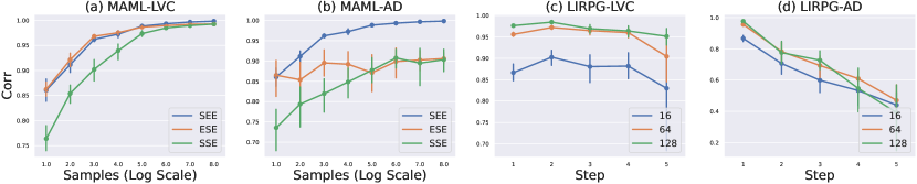
Figure 1: (a, b) Ablation study on sample size and estimators in MAML-RL. “S" is for stochastic estimation while “E" is for exact solution. AD refers to automatic differentiation. (c,d) Ablation study on sample size, steps and estimators in LIRPG.

Firstly, we conduct our ablation studies by comparing the correlation between of meta-gradient with the exact one. The correlation metric, which is determined by bias and variance, can show how the final estimation quality is influenced by these two bias terms. As the quality of stochastic estimators vary from many factors, we conduct this ablation study under extensive combinations of estimation algorithms (including DiCE [12], Loaded-DiCE [8], LVC [29], and pure automatic differentiation in original MAML [10]), learning rates, sample sizes, .etc. Due to the page limit, the results illustrated in Fig. 1(a,b) only include ablation study on sample size using LVC/automatic differentiation and estimation using exact gradients for (III), the outer-loop policy gradient. For the rest ablation study and more evaluation metrics (variance of estimation), refer to Appendix I.1.3.

We start our evaluation by increasing the sample size. For simplicity, we only conduct one inner step here. In Fig. 1(a), we leverage the LVC [29] estimator. We can see that a correct inner-loop policy estimation and/or a Hessian estimation can significantly improve the estimation quality (as $\mathrm{SEE}\approx\mathrm{ESE}>\mathrm{SSE}$ in low sample size case). By increasing the sample size, we can see the gap between them is shrinking, which verifies the finding in Lemma 4.4. In this case the compositional bias correction shares the same importance with the Hessian bais correction ($\mathrm{SEE}\approx\mathrm{ESE}$). We also compare it with the original yet biased gradient estimator of MAML in Fig. 1(b), in which $\mathrm{SEE}>\mathrm{ESE}$ in all sample size settings. In fact, since the gradient estimation is biased, only SEE achieves near $1.0$ correlation provided sufficient samples, again confirms the importance of Hessian bias corrections in Sec. 4.2.

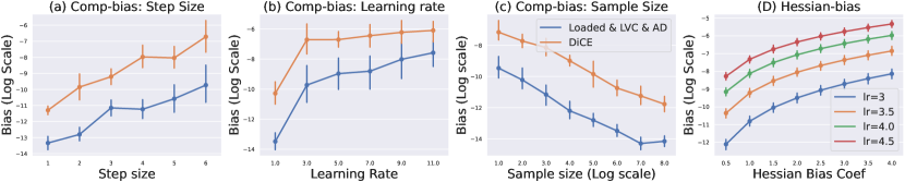
Figure 2: (a, b, c) Ablation study of meta-gradient bias due to the compositional bias in different estimators, step sizes, learning rates. Loaded-DiCE, LVC and AD achieve exactly the same compositional bias because they have the same first-order gradient, (d) Ablation study of meta-gradient bias due to the Hessian bias in different learning rates and Hessian bias coefficients.

Beside the correlation result above, we also add additional experimental results in Fig. 2 over the pure meta-gradient bias term introduced by compositional bias and Hessian bias. It can also be regarded as an empirical verification of our Lemma 4.4 and Theorem 4.5. In Fig. 2 (a, b, c), we mainly study How (a) the inner-loop step size, (b) learning rate and (c) sample size influence final meta-gradient bias. It successfully validates our Lemma 4.4 ($\mathcal{O}\big{(}K\alpha^{K}\hat{\sigma}_{\text{In}}|\tau|^{-0.5}\big{)}$) about the exponential impact from the inner-loop step $K$ (approximately linear relationship between log-scale bias and step size in (a)), the polynomial impact from the learning rate $\alpha$ (approximately Concave downward relationship between log-scale bias and learning rate in (b)) and the polynomial impact from the sample size $\alpha$ (approximately negative linear relationship between log-scale bias and log-scale sample size in (c)). In the second MAML-Hessian experiment, we conduct experiments to verify the polynomial impact $\mathcal{O}\big{(}(K-1)(\hat{\Delta}_{H})^{K-1}\big{)}$ on the meta-gradient bias introduced by the multi-step Hessian estimation bias $\hat{\Delta}_{H}$ (The Concave downward relationship in (d)). In our implementation, we manually add the Hessian bias error into the estimation and control the quantity of it by multiplying different coefficients.

LIRPG. In this setting, we follow the algorithm of intrinsic reward generator presented in [42]. In tabular MDP, we have an additional meta intrinsic reward matrix $\phi$. Starting from $\boldsymbol{\theta}^{0}$, the inner-loop process takes policy gradient based on the new reward matrix $R_{\text{new}}=R+\boldsymbol{\phi}$: $\boldsymbol{\theta}^{i+1}=\boldsymbol{\theta}^{i}+\alpha\nabla_{\boldsymbol{\theta}^{i}}J^{\text{In}}(\boldsymbol{\theta}^{i},\phi),i\in\{0,1...K-1\}$. The meta-gradient estimation of the intrinsic reward matrix $\nabla_{\boldsymbol{\phi}}J^{\text{Out}}(\boldsymbol{\theta}^{K})$ is needed in this case. Note that in the outer loss we use the original reward matrix $R$ so the outer loss is $J^{\text{Out}}(\boldsymbol{\theta}^{K})$ rather than $J^{\text{Out}}(\boldsymbol{\phi},\boldsymbol{\theta}^{K})$. Compared with MAML-RL, the object of meta-update (intrinsic matrix) and the object of inner-update (policy parameters) are different, which help us identify the problem mentioned in Sec. 4.2.

In this case, we choose the LVC and AD estimator. We conduct ablation study on inner-step and sample size shown in Fig. 1(c,d). With more sample size and less step size, the correlation increases for both estimator. Two important features are: (1) With 1-step inner-loop setting, both estimator performs similarly in the correlation. (2) With multi-step inner-loop setting, LVC based estimator can still reach relatively high correlation while MAML-biased estimator directly reaches low correlation after 5-step inner-loop. The phenomenon shown here corresponds exactly to the Hessian estimation issue we discuss in Sec. 4.2 and the bias issue will be more severe with multi-step inner-loop setting.

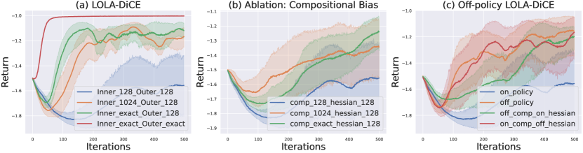
Figure 3: Experiment result of LOLA-DiCE over 10 seeds. The Inner$\_A\_$Outer$\_B$ legend means we use $A$ samples to estimate inner-loop gradient while $B$ samples to estimate outer-loop gradient. The ’exact’ means we use analytical solution of policy gradient instead of estimation.

5.2 Compositional bias/off-policy learning in LOLA

In this subsection, we conduct three experiments on Iterated Prisoner Dilemma (IPD) with the LOLA algorithm to show: (1) The effect brought by different inner/outer estimators. (2) The effect brought compisitional bias (Sec. 4.1) (3) How off-policy correction (Sec. 4.4) can help the LOLA algorithm. Please refer to Appendix I.2.1, I.2.2 for more experimental setting and results.

Ablation on LOLA-DiCE inner/outer estimation. We report the result of conducting ablation study for different inner/outer-loop estimation of LOLA-DiCE in the Fig. 3(a). Here the inner-loop estimation refers to $\nabla_{\boldsymbol{\theta}}J^{\mathrm{In}}(\boldsymbol{\phi},\boldsymbol{\theta})$ while outer-loop estimation refers to $\nabla_{\boldsymbol{\theta}^{1}}J^{\mathrm{Out}}(\boldsymbol{\phi},\boldsymbol{\theta}^{1})$ and $\nabla_{\boldsymbol{\phi}}J^{\mathrm{Out}}(\boldsymbol{\phi},\boldsymbol{\theta}^{1})$. The return shown in Fig. 3(a) reveals us two findings: 1) The inner-loop gradient estimation plays an important role for making LOLA work—the default batch size 128 fails while the batch size 1024 succeeds. 2) The outer-loop gradient estimation is also crucial to the performance of LOLA-Exact. Furthermore, we continue conducting ablation studies on the inner-loop gradient update.

Ablation on compositional bias. Since the unbiased DiCE estimator is used in LOLA-DiCE algorithm, there is no Hessian estimation bias in the LOLA algorithm. Thus, we mainly discuss the problem of compositional bias brought in Fig. 3(b). We also apply the implementation in Sec. 5.1 to decompose meta-gradient estimation with different estimators. Fig. 3(b) show us the ablation study over compositional bias, which reveals that: compositional bias may decrease the performance and by adding more samples or using analytical solution, the performance can start to improve.

Off-policy DiCE and ablation study. We use the off-policy learning to conduct inner-loop update and keep the outer-loop gradient same as before. By combing DiCE and off-policy learning, we have off-policy DiCE $J^{\mathrm{OFF-DICE}}$: $\mathbb{E}_{\boldsymbol{\tau}}\left[\sum_{t=0}^{H-1}\left(\prod_{t^{\prime}=0}^{t}\frac{\pi_{\phi}(\boldsymbol{a}_{t^{\prime}}^{1}\mid\boldsymbol{s}_{t^{\prime}}^{1})\pi_{\theta}(\boldsymbol{a}_{t^{\prime}}^{2}\mid\boldsymbol{s}_{t^{\prime}}^{2})}{\mu_{1}(\boldsymbol{a}_{t^{\prime}}^{1}\mid\boldsymbol{s}_{t^{\prime}}^{1})\mu_{2}(\boldsymbol{a}_{t^{\prime}}^{2}\mid\boldsymbol{s}_{t^{\prime}}^{2})}\right)R_{t}\right],$ where $\phi,\theta$ refer to the current policy, $\mu_{1},\mu_{2}$ refer the behaviour policy for agent 1 and agent 2, respectively. H is the trajectory length and $R$ refers to the reward for agent. Note that the off-policy DiCE here can not only lower the compositional bias by lowering the first-order policy gradient error, but also helps lower the Hessian variance theoretically. By the decomposition trick, we conduct experiments by traversing over all learning settings for (off-off/off-on/on-off/on-on), which are shown at Fig. 3(d). Comparisons between different settings verify that off-policy DiCE can increase performance by either lowering the compositional bias, or the hessian variance, or both.

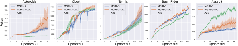
Figure 4: Experimental results on Atari game over 5 random seeds.

5.3 Multi-step Hessian correction on MGRL

Finally, we conduct experiment over MGRL [39]. See Appendix I.3.1 and I.3.2 for experimental settings. When applying the LVC estimator in MGRL, we get the new inner-loop update equation: $\mathbb{E}_{\boldsymbol{\tau}\sim p(\boldsymbol{\tau};\boldsymbol{\theta})}\left[\sum_{t=0}^{H-1}\frac{\nabla_{\boldsymbol{\theta}}\pi_{\boldsymbol{\theta}}(\boldsymbol{a}_{t}|\boldsymbol{s}_{t})}{\perp\pi_{\boldsymbol{\theta}}(\boldsymbol{a}_{t}|\boldsymbol{s}_{t})}\left(g_{\boldsymbol{\phi}}(\boldsymbol{\tau})-v_{\boldsymbol{\theta}}(\boldsymbol{s}_{t})\right)\right],$ where $\boldsymbol{\phi}=(\gamma,\lambda)$ refer to meta-paramters and $\theta$ refers to the RL policy, $g_{\boldsymbol{\phi}}(\tau)$ denotes $\lambda$-return, $v_{\boldsymbol{\theta}}(s_{t})$ denotes value prediction. We conduct experiment on eight environments of Atari games. We follow previous work [4] to use the "discard" strategy in which we conduct multiple virtual inner-loop updates for meta gradient estimation. This strategy is designed to keep the inner learning update unchanged.

In Fig. (4), we show five environments comparing three variants of algorithm: 1) Baseline Advantage Actor-critic(A2C) algorithm [25]; 2) 3-step MGRL + A2C; 4) 3-step MGRL + A2C + LVC correction. The "3-step" means we take 3 inner-loop RL virtual updates for calculating meta-gradient. Refer to Appendix I.3.3 for experimental results on all eight environments. Compared with 3-step MGRL, the MGRL with LVC correction can substantially improves the performance, which validates the effectiveness of the multi-step Hessian correction in Sec. 4.4 for handling meta-gradient estimation bias and bring in better hyperparameter-tuning in RL. Note that the fact that A2C algorithms can achieve better results compared with 3-step MGRL is consistent with the results in [39].

6 Conclusion

In this paper, we introduce a unified framework for studying generic meta-gradient estimations in gradient-based Meta-RL. Based on this framework, we offer two theoretical insights that 1) the compositional bias has an upper bound of $\mathcal{O}\big{(}K\alpha^{K}\hat{\sigma}_{\text{In}}|\tau|^{-0.5}\big{)}$ with respect to the inner-loop update step $K$, the learning rate $\alpha$, the estimate variance $\hat{\sigma}^{2}_{\text{In}}$ and the sample size $|\tau|$, and 2) the multi-step Hessian bias $\hat{\Delta}_{H}$ has a polynomial impact of $\mathcal{O}\big{(}(K-1)(\hat{\Delta}_{H})^{K-1}\big{)}$. To validate our theoretical discoveries, we conduct a comprehensive list of ablation studies. Empirical results over tabular MDP, LOLA-DiCE and MGRL validate our theories and the effectiveness of correction methods. We believe our work can inspire more future work on unbiased meta-gradient estimations in GMRL.

Checklist

1. For all authors…

   1. Do the main claims made in the abstract and introduction accurately reflect the paper’s contributions and scope? [Yes]

   2. Did you describe the limitations of your work? [Yes] See Appendix B.

   3. Did you discuss any potential negative societal impacts of your work? [N/A]

   4. Have you read the ethics review guidelines and ensured that your paper conforms to them? [Yes]

2. If you are including theoretical results…

   1. Did you state the full set of assumptions of all theoretical results? [Yes] See Sec. 4

   2. Did you include complete proofs of all theoretical results? [Yes] See Appendix F and Appendix G

3. If you ran experiments…

   1. Did you include the code, data, and instructions needed to reproduce the main experimental results (either in the supplemental material or as a URL)? [Yes]

   2. Did you specify all the training details (e.g., data splits, hyperparameters, how they were chosen)? [Yes] , See Appendix I

   3. Did you report error bars (e.g., with respect to the random seed after running experiments multiple times)? [Yes] , See Fig. 1, 3, 4.

   4. Did you include the total amount of compute and the type of resources used (e.g., type of GPUs, internal cluster, or cloud provider)? [Yes] See Appendix I

4. If you are using existing assets (e.g., code, data, models) or curating/releasing new assets…

   1. If your work uses existing assets, did you cite the creators? [Yes]

   2. Did you mention the license of the assets? [Yes]

   3. Did you include any new assets either in the supplemental material or as a URL? [No]

   4. Did you discuss whether and how consent was obtained from people whose data you’re using/curating? [N/A]

   5. Did you discuss whether the data you are using/curating contains personally identifiable information or offensive content? [Yes]

5. If you used crowdsourcing or conducted research with human subjects…

   1. Did you include the full text of instructions given to participants and screenshots, if applicable? [N/A]

   2. Did you describe any potential participant risks, with links to Institutional Review Board (IRB) approvals, if applicable? [N/A]

   3. Did you include the estimated hourly wage paid to participants and the total amount spent on participant compensation? [N/A]

Supplementary Material

The supplementary material is organized as follows. Appendix A offers more algorithm illustration for the 4 topics we discuss in Sec. 3. In Appendix B we discuss our choice for EPG formulation and the truncated setting in GMRL. In Appendix C we briefly summarise biased Hessian estimation issue in MAML-RL mentioned in Section 4.2, In Appendix D we illustrate how realistic are Assumption 4.1-4.3 of Section 4. Appendices E, F and G contain the proofs for the results presented in the paper. In Appendix H we provide statements and proofs for some auxiliary lemmas which are instrumental for the main results. For convenience of the reader, before each proof we also restate the corresponding theorem. Finally, in Appendix I we present additional experiments results.

Appendix A More topics on GMRL

A.1 Few-shot Reinforcement Learning

One important research field in Meta Reinforcement Learning is few-shot Reinforcement Learning. The main objective of this research field is to enable Reinforcement Learning agent with fast adaptation ability. Instead of thousands of interactions in traditional Reinforcement Learning algorithms, agent in few-shot setting is only allowed to interact with the new environment for a few trajectories. One of the most classical gradient based algorithms in this field is Model Agnostic Meta Learning (MAML-RL). [10] aims at learning neural network’s initial parameters for fast adaptation on new environments. It assumes distribution $\rho(\mathcal{T})$ over RL environment $\mathcal{T}$ and tries to optimise $\boldsymbol{\theta}$ which leads to high-performing updated policy $\boldsymbol{\theta}^{\prime}$. The objective equation for one-step MAML-RL can be shown as follows:

$$J(\boldsymbol{\theta})=\mathbb{E}_{\mathcal{T}\sim\rho(\mathcal{T})}\left[\mathbb{E}_{\boldsymbol{\boldsymbol{\tau}}^{\prime}\sim P_{\mathcal{T}}\left(\boldsymbol{\boldsymbol{\tau}}^{\prime}\mid\boldsymbol{\theta}^{\prime}\right)}\left[R\left(\boldsymbol{\boldsymbol{\tau}}^{\prime}\right)\right]\right]\quad$$ (11)

$$\text{ with }\quad\boldsymbol{\theta}^{\prime}=\boldsymbol{\theta}+\alpha\nabla_{\boldsymbol{\theta}}\mathbb{E}_{\boldsymbol{\boldsymbol{\tau}}\sim P_{\mathcal{T}}(\boldsymbol{\boldsymbol{\tau}}\mid\boldsymbol{\theta})}[R(\boldsymbol{\boldsymbol{\tau}})]$$

where in practice we use the limited trajectories sampled from the new environment to estimate $\nabla_{\boldsymbol{\theta}}\mathbb{E}_{\boldsymbol{\boldsymbol{\tau}}\sim P_{\mathcal{T}}(\boldsymbol{\boldsymbol{\tau}}\mid\boldsymbol{\theta})}[R(\boldsymbol{\boldsymbol{\tau}})]$. During training, by estimating meta policy gradient $\nabla_{\boldsymbol{\theta}}J(\boldsymbol{\theta})$, MAML can conduct meta update on the initial policy parameters.

In the scope of Eq. (2), MAML-RL optimizes over meta initial parameters to maximize the return of one-step adapted policy: $\boldsymbol{\theta}^{\prime}=\boldsymbol{\theta}+\alpha\nabla_{\boldsymbol{\theta}}J^{\text{In}}(\boldsymbol{\theta})$. In MAML-RL, $J^{\text{Out}}(\boldsymbol{\phi},\boldsymbol{\theta}^{\prime})$ degenerates to $J^{\text{Out}}(\boldsymbol{\theta}^{\prime})$ and $\boldsymbol{\phi}$ and $\boldsymbol{\theta}$ represent the same initial parameters. The meta-gradient can be derived with the following equation:

$$\nabla_{\boldsymbol{\theta}}J(\boldsymbol{\theta})=\nabla_{\boldsymbol{\theta}}\boldsymbol{\theta}^{\prime}\nabla_{\boldsymbol{\theta}^{\prime}}J^{\text{Out }}\left(\boldsymbol{\theta}^{\prime}\right),\nabla_{\boldsymbol{\theta}}\boldsymbol{\theta}^{\prime}=I+\alpha\nabla_{\boldsymbol{\theta}}^{2}J^{\text{In}}(\boldsymbol{\theta})$$ (12)

A.2 Meta-gradient in Opponent Shaping

Opponent shaping [11, 19, 22] is a powerful tool in multi-agent learning process for different purposes. For instance, Foerster et al. [11] and Letcher et al. [22] have shown that putting other-players learning dynamic into self-learning process can bring in cooperation behaviors, which may help to reach better social welfare compared with purely independent learning. Meta-gradient estimation is needed when ego-agent takes derivatives of other-agent policy gradient step. Learning with Opponent-Learning Awareness (LOLA) [11] proposed a new learning objective by including an additional term accounting for the impact of ego policy to the anticipated opponent gradient update. Specifically, in the two-player setting, with agent 1 policy $\boldsymbol{\phi}$ and agent 2 policy $\boldsymbol{\theta}$, the traditional independent learning (IL) and 1-step LOLA algorithm can result in different updates for agent 1:

$$\boldsymbol{\phi}^{\prime}_{\text{IL}}=\boldsymbol{\phi}+\beta\nabla_{\boldsymbol{\phi}}J^{\text{Out}}(\boldsymbol{\phi},\boldsymbol{\theta})$$ (13)

$$\boldsymbol{\phi}^{\prime}_{\text{LOLA}}=\boldsymbol{\phi}+\beta\nabla_{\boldsymbol{\phi}}J^{\text{Out}}(\boldsymbol{\phi},\boldsymbol{\theta}^{\prime})$$

$$\text{where }\boldsymbol{\theta}^{\prime}=\boldsymbol{\theta}+\alpha\nabla_{\boldsymbol{\theta}}J^{\text{In}}(\boldsymbol{\phi},\boldsymbol{\theta})$$

Where $\beta$ refers to the outer learning rate and $J^{\text{In/Out}}$ refers to the value function for agent 2 and agent 1 respectively. For meta-agent 1 with parameters $\boldsymbol{\phi}$, it will optimise its return over one-step-lookahead opponent parameters $\boldsymbol{\theta}^{\prime}$. Thus the meta-gradient of meta-agent corresponds exactly to Eq. (2) with $\nabla_{\boldsymbol{\phi}}{\boldsymbol{\theta}^{\prime}}=\alpha\nabla_{\boldsymbol{\phi}}\nabla_{\boldsymbol{\theta}}J^{\text{In}}(\boldsymbol{\phi},\boldsymbol{\theta})$. Note that this one-step-lookahead is a just virtual update considered in the optimisation of agent 1. Agent 2 can also choose this LOLA update by conducting one-step-lookahead over agent 1.

A.3 Single-lifetime Meta-gradient RL

In this setting, the main objective is to self-tune the meta parameters ($\gamma$ in [39]) or meta models (intrinsic model in [42]) along with the underlying normal RL updates. It is called online because it only involves one single RL life-time. This research field is also related with online hyperparameter optimisation in supervised learning such as [2, 14]. Xu et al. [39] proposed meta-gradient reinforcement learning (MGRL) to tune the discount factor $\gamma$ and bootstrapping parameter $\lambda$ in an online manner. It tries to differentiate through one RL inner update to optimize the meta-parameters and maximise one-step policy return.

$$\max_{\boldsymbol{\eta}}V^{\pi_{\boldsymbol{\theta}^{\prime}}}, \text{where }\boldsymbol{\theta}^{\prime}=\boldsymbol{\theta}+\alpha\nabla_{\boldsymbol{\theta}}J(\boldsymbol{\tau},\boldsymbol{\theta},\boldsymbol{\eta}),\text{and}$$ (14)

$$\nabla_{\boldsymbol{\theta}}J(\boldsymbol{\tau},\boldsymbol{\theta},\boldsymbol{\eta}) =\left(g_{\boldsymbol{\eta}}(\boldsymbol{\tau})-v_{\boldsymbol{\theta}}(S)\right)\nabla_{\boldsymbol{\theta}}\log\pi_{\boldsymbol{\theta}}(A\mid S)$$

$$+\left(g_{\boldsymbol{\eta}}(\boldsymbol{\tau})-v_{\boldsymbol{\theta}}(S)\right)\nabla_{\boldsymbol{\theta}}v_{\boldsymbol{\theta}}(S)$$

$$+\nabla_{\boldsymbol{\theta}}H\left(\pi_{\boldsymbol{\theta}}(\cdot\mid S)\right)$$

where $\eta$ refers to $(\gamma,\lambda)$, $\boldsymbol{\tau}$ refers to trajectories, $g_{\boldsymbol{\eta}}$, $v_{\boldsymbol{\theta}}$, H represent GAE estimation, value function and entropy respectively. Eq. (14) combines actor loss, critic loss and entropy loss, which are commonly used in typical Actor-Critic [25] algorithms. Specifically, the meta parameters $(\gamma,\lambda)$ corresponds to $\boldsymbol{\phi}$ in Eq. (2) . After the policy parameters $\boldsymbol{\theta}$ take one policy gradient update to become $\boldsymbol{\theta}^{\prime}$($\boldsymbol{\theta}^{\prime}=\boldsymbol{\theta}+\alpha\nabla_{\boldsymbol{\theta}}J^{\text{In}}(\boldsymbol{\theta},\boldsymbol{\phi})$), we can calculate the meta-gradient by backpropogating from $J^{\text{Out}}$ to meta parameters. In MGRL, $J^{\text{Out}}(\boldsymbol{\phi},\boldsymbol{\theta}^{\prime})$ degenerates to $J^{\text{Out}}(\boldsymbol{\theta}^{\prime})$. The meta-gradient can be shown as:

$$\nabla_{\boldsymbol{\phi}}J(\boldsymbol{\phi})=\nabla_{\boldsymbol{\phi}}\boldsymbol{\theta}^{\prime}\nabla_{\boldsymbol{\theta}^{\prime}}J^{\text{Out }}\left(\boldsymbol{\theta}^{\prime}\right),\nabla_{\boldsymbol{\phi}}\boldsymbol{\theta}^{\prime}=\alpha\nabla_{\boldsymbol{\phi}}\nabla_{\boldsymbol{\theta}}J^{\text{In}}(\boldsymbol{\theta},\boldsymbol{\phi})$$ (15)

Here for simplicity we omit the critic and entropy loss. Usually work in this research field only conduct one-step inner-loop update before taking meta update. Some recent works such as [34, 4] have also shown that multi-step online meta-gradient can achieve better performance.

A.4 Multi-lifetime Meta-gradient RL

Existing work like [26, 43, 40, 9] are trying to learn some fundamental/generalizable meta module across different environments such as a neural RL algorithm in [26](LPG). An important feature of multi-lifetime Meta-gradient RL is that it inherently needs multi-step inner-loop to account for the effect of fundamental meta module over the RL process. The objective of LPG is to learn a neural network based RL algorithm, by which a RL agent can be properly trained. The mathmatical formulation can be shown as follows:

$$J(\boldsymbol{\phi})=\mathbb{E}_{\mathcal{T}\sim\rho(\mathcal{T})}\left[\mathbb{E}_{\boldsymbol{\tau}^{K}\sim P_{\mathcal{T}}\left(\boldsymbol{\tau}^{K}\mid\theta^{K}\right)}\left[R\left(\boldsymbol{\tau}^{K}\right)\right]\right],\text{with}$$ (16)

$$\theta^{i}=\theta^{i-1}+\alpha\nabla_{\theta^{i-1}}\mathbb{E}_{\boldsymbol{\tau}\sim P_{\mathcal{T}}(\boldsymbol{\tau}\mid\theta^{i-1})}[f_{\boldsymbol{\phi}}(\boldsymbol{\tau})]$$ (17)

where $f_{\boldsymbol{\phi}}(\boldsymbol{\tau})$ is the output of meta-network $\boldsymbol{\phi}$ for conducting inner-loop neural policy gradient and $k$ can be large to show the long-range impact brought by neural RL algorithm. We omit the kl inner loss used in [26] for simplicity. In the scope of Eq. (1), $J^{\text{In/Out}}$ refers to the value function, $\boldsymbol{\theta}$ represents the RL agent policy parameters and $\boldsymbol{\phi}$ is the meta-parameter of neural RL algorithm. Most of works are under a multi-task/environment (or a distribution over environment) and multi-lifetime setting. [40] is a special case in these work because it is also under the online setting. We believe the main reason is that the training iterations/sample complexity in [40] is real large (1e9) and makes it become a special case of ’multi-lifetime’ setting.

Appendix B Discussion of expected policy gradient (EPG) formulation and truncated setting

We discuss 4 research topics in Section 3: few-shot RL(MAML-RL), opponent shaping(LOLA-DiCE), online meta gradient RL(MGRL) and meta gradient based inverse design(LPG). And we need to discuss how this multi-step EPG inner-loop formulation differs in these topics. Though they all need meta policy gradient estimation, the differences between setting and final objective require us to discuss them separately.

Different setting: MAML-RL and most inverse design algorithms are under multi-lifetime setting which can renew an environment and restart the RL training from the very beginning. Work in online meta gradient RL/LOLA only happen in a single lifetime RL process. There only exists one RL training process.

Different objectives: For MAML-RL, the main objective is to maximise the return of few-step adapted policy. Thus the objective corresponds exactly to few-step inner-loop formulation. However, for topics beyond few-shot RL, in most case they need to measure the influence of meta module over RL final (after thousands of steps) performance.

There are two important issues in this EPG formulation. The first one is that it assumes an expected policy gradient inner-loop update. And the second one is because we only consider few-step inner-loop update so they are under a truncated estimation setting which might bring in bias. Recently, one work [36] argues that: (1) the general unbiased meta gradient for MAML-RL ([10]) and Online Meta Gradient ([39],[42]) should be the K-sample inner-loop meta gradient shown in E-MAML [1] rather than the expected policy gradient inner-loop meta gradient used in many recent work [23, 29, 33]. (2) The gradient estimator in online meta gradient utilise truncated optimization and the unbiased meta gradient should be the one in untruncated setting.

Overall we agree that: (1) The K-sample inner-loop meta gradient estimator is unbiased for MAML-RL problem when sampled policy gradient are used. (2) To learn an schedule (rather than a global meta module) of meta-parameter/meta-module for MGRL or to learn some fundamental concepts in inverse-design, the gradient estimator in untruncated setting is unbiased. However, we argue that (1) For MAML-related problem, the variance of sampling correction term in K-sample inner-loop meta gradient estimator is large because it needs to sum up all $k$ terms and that is why [36] proposes to use one coefficient to control. The EPG can achieve lower variance estimation and perform better empirically [29] (2) For meta gradient based inverse design with multi-lifetime, the few-step meta gradient estimation under truncated setting is biased.

However, in online meta gradient setting (MGRL) or online opponent modelling (LOLA) with single-lifetime, things are completely different thus a direct transform of K-sample inner-loop formulation from MAML to MGRL might not be that straightforward. There exists a large gap between the implementation of online meta gradient algorithm and the final objective (meta-module/hyperparameters schedule) we may wish. First, it’s an online setting so the multiple lifetime setting where the algorithm can restart from the very beginning and reiterate the whole process is banned here. This makes the estimation of unbiased meta gradient impossible because the algorithm cannot access to the future dynamic for gradient estimation. The experiments with multi-lifetime training in [36] is in fact out of the scope of online meta gradient setting and are more like meta gradient based inverse design. Second, in implementation of MGRL they only maintain one running $\gamma$ or intrinsic model rather than multiple meta modules as a real schedule needs. Also, recently there exist one work [4] discussing multi-step MGRL and use one fixed meta parameters rather than a schedule for multi-step inner-loop, which may show a different understanding about untruncated gradient. In all, we believe that what online meta algorithm/opponent shaping like MGRL or LOLA optimizes and what the best they can achieve in such online setting are still open questions and remain to be further explored. It is really hard to simply formulate the unbiased meta gradient since the gap between implementation and objective is still not clear.

Thus, in our paper, we still focuses on the previous work (MAML/MGRL and LOLA) objectives with EPG inner-loop setting and use its meta gradient as our target gradient. All bias term we discuss is the bias w.r.t. the expected meta gradient in this EPG inner-loop and truncated setting. That is our work’s limitation and we leave more things for future work: (1)The gap between EPG inner-loop meta gradient and K-sample inner-loop meta gradient in MAML-RL related problem. (2) The gap between truncated EPG inner-loop meta gradient and what the best gradient estimation we can get in online meta gradient/opponent shaping. (3) The gap between truncated EPG inner-loop meta gradient and the untruncated gradient in meta gradient based inverse design.

Appendix C Brief summary on biased Hessian estimation in MAML-RL

We will briefly introduce the reasons of biased Hessian estimation with automatic differentiation in one-step MAML-RL. Firstly, we can derive the analytic form of $\boldsymbol{\theta}^{1}$ and $\nabla_{\boldsymbol{\theta}^{0}}\boldsymbol{\theta}^{1}$

$$\boldsymbol{\theta}^{1}=\boldsymbol{\theta}^{0}+\alpha\mathbb{E}_{\boldsymbol{\tau}\sim p(\boldsymbol{\tau};\boldsymbol{\theta}^{0})}[\nabla_{\boldsymbol{\theta}^{0}}\log\pi(\boldsymbol{\tau})\mathcal{R}(\boldsymbol{\tau})]$$ (18)

$$\nabla_{\boldsymbol{\theta}^{0}}\boldsymbol{\theta}^{1}=I+\mathbb{E}_{\boldsymbol{\tau}\sim p(\boldsymbol{\tau};\boldsymbol{\theta}^{0})}\left[\mathcal{R}(\boldsymbol{\tau})\left(\nabla_{\boldsymbol{\theta}^{0}}^{2}\log\pi_{\boldsymbol{\theta}^{0}}(\boldsymbol{\tau})+\nabla_{\boldsymbol{\theta}^{0}}\log\pi_{\boldsymbol{\theta}^{0}}(\boldsymbol{\tau})\nabla_{\boldsymbol{\theta}^{0}}\log\pi_{\boldsymbol{\theta}^{0}}(\boldsymbol{\tau})^{\top}\right)\right]$$ (19)

Typically we need to use trajectory samples $\boldsymbol{\tau}_{n}$ to estimate the policy gradient, we can get the adapted policy estimate.

$$\hat{\boldsymbol{\theta}}^{1}=\boldsymbol{\theta}^{0}+\alpha\frac{1}{N}\sum_{\boldsymbol{\tau}_{n}}\sum_{t=0}^{H-1}\nabla_{\boldsymbol{\theta}}\log\pi_{\boldsymbol{\theta}}(\boldsymbol{a}^{n}_{t}\mid\boldsymbol{s}^{n}_{t})\left(\sum_{t^{\prime}=0}^{H}\gamma^{t}r\left(\boldsymbol{s}^{n}_{t^{\prime}},\boldsymbol{a}^{n}_{t^{\prime}}\right)\right)$$ (20)

Finally, implementation of MAML-RL derives the gradient estimate by automatic differentation. The corresponding estimation is biased:

$$\mathbb{E}[\nabla_{\boldsymbol{\theta}^{0}}\hat{\boldsymbol{\theta}}^{1}] =I+\alpha\mathbb{E}_{\boldsymbol{\tau}\sim p(\boldsymbol{\tau};\boldsymbol{\theta}^{0})}\left[\frac{1}{N}\sum_{\boldsymbol{\tau}_{n}}\sum_{t=0}^{H-1}\nabla_{\boldsymbol{\theta}^{0}}^{2}\log\pi_{\boldsymbol{\theta}^{0}}(\boldsymbol{a}^{n}_{t}\mid\boldsymbol{s}^{n}_{t})\left(\sum_{t^{\prime}=0}^{H}\gamma^{t}r(\boldsymbol{s}^{n}_{t^{\prime}},\boldsymbol{a}^{n}_{t^{\prime}})\right)\right]$$ (21)

$$=I+\alpha\mathbb{E}_{\boldsymbol{\tau}\sim p(\boldsymbol{\tau};\boldsymbol{\theta}^{0})}\left[\mathcal{R}(\boldsymbol{\tau})\nabla_{\boldsymbol{\theta}}^{2}\log\pi_{\boldsymbol{\theta}^{0}}(\boldsymbol{\tau})\right]\not=\nabla_{\boldsymbol{\theta}^{0}}\boldsymbol{\theta}^{1}$$

The main reason of biased Hessian estimation is that automatic differentiation tools only consider the dependency of $\boldsymbol{\theta}$ in $\nabla_{\boldsymbol{\theta}}\log\pi_{\boldsymbol{\theta}}$ while ignoring the dependency in expectation $\mathbb{E}_{\boldsymbol{\tau}\sim p(\boldsymbol{\tau};\boldsymbol{\theta}^{0})}$. In practice, the $\mathbb{E}_{\boldsymbol{\tau}\sim p(\boldsymbol{\tau};\boldsymbol{\theta}^{0})}$ is represented by trajectory sampling so the gradient term $\nabla_{\boldsymbol{\theta}}\mathbb{E}_{\boldsymbol{\tau}\sim p(\boldsymbol{\tau};\boldsymbol{\theta}^{0})}$ is 0 using automatic differentiation. We need to add additional terms to further derive the gradient $\nabla_{\boldsymbol{\theta}}\mathbb{E}_{\boldsymbol{\tau}\sim p(\boldsymbol{\tau};\boldsymbol{\theta}^{0})}$ brought by sampling dependency.

Appendix D Limitations on Assumptions

Assumption 4.1-4.3 are standard assumptions used in various theoretical MAML-RL papers [6, 7, 18]. The Lipschitz continuity assumptions in Assumption 4.1 make sure we can work with nonconvex inner and outer objectives. The unbiased first-order gradient estimators assumptions in Assumption 4.2 can highlight our findings on two source of biases, which is also a plausible assumption in GMRL settings. As typically adopted in the analysis for stochastic optimization, we make the bounded-variance assumption in Assumption 4.3. Assumption 4.1-4.3 can be conveniently verified for e.g., inner-loop RL optimization in tabular MDP settings (finite state space and action space) with soft-max parameterisation of the policy, where $\pi_{\boldsymbol{\theta}}(\boldsymbol{a}\mid\boldsymbol{s})\propto\exp(\boldsymbol{\theta}(\boldsymbol{s},\boldsymbol{a}))$ with parameter $\boldsymbol{\theta}={\boldsymbol{\theta}(\boldsymbol{s},\boldsymbol{a})}$. But in large-scale RL settings like atari games, Assumption 4.1-4.3 will not hold anymore.

Appendix E Proof of Proposition in Section 3

In this section, we provide the proof for Proposition 3.1 in Section 3.

E.1 Proof of Proposition 3.1

See 3.1

Proof.

According to post-update inner parameters $\boldsymbol{\theta}^{K}=\boldsymbol{\theta}^{0}+\alpha\sum_{i=0}^{K-1}\nabla_{\boldsymbol{\theta}^{i}}J^{\text{In}}(\boldsymbol{\phi},\boldsymbol{\theta}^{i})$ and the fact that $\nabla_{\boldsymbol{\theta}^{i}}J^{\text{In}}(\boldsymbol{\phi},\boldsymbol{\theta}^{i})$ is differentiable w.r.t. $\boldsymbol{\phi}$, we can treat $\boldsymbol{\theta}^{K}$ as a differentiable function w.r.t. $\boldsymbol{\phi}$. Based on the chain rule, we can get

$$\nabla_{\boldsymbol{\phi}}J^{K}(\boldsymbol{\phi}) =\nabla_{\boldsymbol{\phi}}J^{\text{Out}}(\boldsymbol{\phi},\boldsymbol{\theta}^{K})+\nabla_{\boldsymbol{\phi}}\boldsymbol{\theta}^{K}\nabla_{\boldsymbol{\theta}^{K}}J^{\text{Out }}(\boldsymbol{\phi},\boldsymbol{\theta}^{K})$$ (22)

Based on the iterative updates that $\boldsymbol{\theta}^{i+1}=\boldsymbol{\theta}^{i}+\alpha\nabla_{\boldsymbol{\theta}^{i}}J^{In}(\boldsymbol{\phi},\boldsymbol{\theta}^{i})$, for $i=0,\ldots,K-1$ and similarly treat $\boldsymbol{\theta}^{i}$ as a differentiable function w.r.t. $\boldsymbol{\phi}$, we have

$$\nabla_{\boldsymbol{\phi}}\boldsymbol{\theta}^{i+1}= \nabla_{\boldsymbol{\phi}}\boldsymbol{\theta}^{i}+\alpha\nabla_{\boldsymbol{\phi}}\nabla_{\boldsymbol{\theta}^{i}}J^{\text{In}}(\boldsymbol{\phi},\boldsymbol{\theta}^{i})+\alpha\nabla_{\boldsymbol{\phi}}\boldsymbol{\theta}^{i}\nabla^{2}_{\boldsymbol{\theta}^{i}}J^{\text{In}}(\boldsymbol{\phi},\boldsymbol{\theta}^{i})$$ (23)

$$= \nabla_{\boldsymbol{\phi}}\boldsymbol{\theta}^{i}\left(I+\alpha\nabla^{2}_{\boldsymbol{\theta}^{i}}J^{\text{In}}(\boldsymbol{\phi},\boldsymbol{\theta}^{i})\right)+\alpha\nabla_{\boldsymbol{\phi}}\nabla_{\boldsymbol{\theta}^{i}}J^{\text{In}}(\boldsymbol{\phi},\boldsymbol{\theta}^{i})$$

Telescoping the above equality over $i$ from 0 to $K-1$, we can get

$$\nabla_{\boldsymbol{\phi}}\boldsymbol{\theta}^{K}= \nabla_{\boldsymbol{\phi}}\boldsymbol{\theta}^{0}\prod_{i=0}^{K-1}\left(I+\alpha\nabla^{2}_{\boldsymbol{\theta}^{i}}J^{\text{In}}(\boldsymbol{\phi},\boldsymbol{\theta}^{i})\right)+\alpha\sum_{i=0}^{K-1}\nabla_{\boldsymbol{\phi}}\nabla_{\boldsymbol{\theta}^{i}}J^{\text{In}}(\boldsymbol{\phi},\boldsymbol{\theta}^{i})\prod_{j=i+1}^{K-1}\left(I+\alpha\nabla^{2}_{\boldsymbol{\theta}^{j}}J^{\text{In}}(\boldsymbol{\phi},\boldsymbol{\theta}^{j})\right)$$ (24)

$$= \alpha\sum_{i=0}^{K-1}\nabla_{\boldsymbol{\phi}}\nabla_{\boldsymbol{\theta}^{i}}J^{\text{In}}(\boldsymbol{\phi},\boldsymbol{\theta}^{i})\prod_{j=i+1}^{K-1}\left(I+\alpha\nabla^{2}_{\boldsymbol{\theta}^{j}}J^{\text{In}}(\boldsymbol{\phi},\boldsymbol{\theta}^{j})\right)$$

Combining Eq. (22) and Eq. (24) finishes the proof of Proposition 3.1. ∎

Appendix F Proof of Lemma in Section 4

F.1 Proof of Lemma 4.4

See 4.4

Proof.

In expected policy gradient inner-loop update setting, the iterative updates takes the form

$$\boldsymbol{\theta}^{i+1}=\boldsymbol{\theta}^{i}+\alpha\nabla_{\boldsymbol{\theta}^{i}}J^{\text{In}}(\boldsymbol{\phi},\boldsymbol{\theta}^{i}),\text{ }i=0,\ldots,K-1$$ (25)

In Eq. (4), $\boldsymbol{\theta}^{i+1}$ are estimated using samples $\boldsymbol{\tau}^{0:i}_{0}$, then we have

$$\hat{\boldsymbol{\theta}}^{i+1}=\hat{\boldsymbol{\theta}}^{i}+\alpha\nabla_{\hat{\boldsymbol{\theta}}^{i}}\hat{J}^{\text{In}}(\boldsymbol{\phi},\hat{\boldsymbol{\theta}}^{i},\boldsymbol{\tau}^{i}_{0}),\text{ }\hat{\boldsymbol{\theta}}^{0}=\boldsymbol{\theta}^{0},\text{ }i=0,\ldots,K-1$$ (26)

According to the assumption that non-linear compositional vector-valued $f(\cdot)$ is Lipschitz continuous with constant $C_{0}$, we can get

$$\mathbb{E}_{\boldsymbol{\tau}^{0:K-1}_{0}}[\|f(\hat{\boldsymbol{\theta}}^{K})-f(\boldsymbol{\theta}^{K})\|]\leq C_{0}\mathbb{E}_{\boldsymbol{\tau}^{0:K-1}_{0}}\left[\left\|\hat{\boldsymbol{\theta}}^{K}-\boldsymbol{\theta}^{K}\right\|\right]$$ (27)

Based on Eq. (25) and Eq. (26), we can get

$$\mathbb{E}_{\boldsymbol{\tau}^{0:K-1}_{0}}\left[\left\|\hat{\boldsymbol{\theta}}^{K}-\boldsymbol{\theta}^{K}\right\|\right]$$ (28)

$$= \mathbb{E}_{\boldsymbol{\tau}^{0:K-1}_{0}}\left[\bigg{\|}\hat{\boldsymbol{\theta}}^{K-1}-\boldsymbol{\theta}^{K-1}+\alpha\nabla_{\boldsymbol{\theta}^{K-1}}J^{\text{In}}(\boldsymbol{\phi},\boldsymbol{\theta}^{K-1})-\alpha\nabla_{\hat{\boldsymbol{\theta}}^{K-1}}\hat{J}^{\text{In}}(\boldsymbol{\phi},\hat{\boldsymbol{\theta}}^{K-1},\boldsymbol{\tau}^{K-1}_{0})\bigg{\|}\right]$$

$$\overset{(i)}{\leq} \mathbb{E}_{\boldsymbol{\tau}^{0:K-1}_{0}}\left[\bigg{\|}\hat{\boldsymbol{\theta}}^{K-1}-\boldsymbol{\theta}^{K-1}\bigg{\|}\right]+\alpha\mathbb{E}_{\boldsymbol{\tau}^{0:K-1}_{0}}\left[\bigg{\|}\nabla_{\boldsymbol{\theta}^{K-1}}J^{\text{In}}(\boldsymbol{\phi},\boldsymbol{\theta}^{K-1})-\mathbb{E}_{\boldsymbol{\tau}^{K-1}_{0}}[\nabla_{\hat{\boldsymbol{\theta}}^{K-1}}\hat{J}^{\text{In}}(\boldsymbol{\phi},\hat{\boldsymbol{\theta}}^{K-1},\boldsymbol{\tau}^{K-1}_{0})]\bigg{\|}\right]+$$

$$\alpha\mathbb{E}_{\boldsymbol{\tau}^{0:K-1}_{0}}\left[\bigg{\|}\mathbb{E}_{\boldsymbol{\tau}^{K-1}_{0}}[\nabla_{\hat{\boldsymbol{\theta}}^{K-1}}\hat{J}^{\text{In}}(\boldsymbol{\phi},\hat{\boldsymbol{\theta}}^{K-1},\boldsymbol{\tau}^{K-1}_{0})]-\nabla_{\hat{\boldsymbol{\theta}}^{K-1}}\hat{J}^{\text{In}}(\boldsymbol{\phi},\hat{\boldsymbol{\theta}}^{K-1},\boldsymbol{\tau}^{K-1}_{0})\bigg{\|}\right]$$

$$\leq \mathbb{E}_{\boldsymbol{\tau}^{0:K-1}_{0}}\left[\bigg{\|}\hat{\boldsymbol{\theta}}^{K-1}-\boldsymbol{\theta}^{K-1}\bigg{\|}\right]+\alpha c_{2}\mathbb{E}_{\boldsymbol{\tau}^{0:K-1}_{0}}\left[\bigg{\|}\hat{\boldsymbol{\theta}}^{K-1}-\boldsymbol{\theta}^{K-1}\bigg{\|}\right]+$$

$$\alpha\mathbb{E}_{\boldsymbol{\tau}^{0:K-1}_{0}}\left[\bigg{\|}\mathbb{E}_{\boldsymbol{\tau}^{K-1}_{0}}[\nabla_{\hat{\boldsymbol{\theta}}^{K-1}}\hat{J}^{\text{In}}(\boldsymbol{\phi},\hat{\boldsymbol{\theta}}^{K-1},\boldsymbol{\tau}^{K-1}_{0})]-\nabla_{\hat{\boldsymbol{\theta}}^{K-1}}\hat{J}^{\text{In}}(\boldsymbol{\phi},\hat{\boldsymbol{\theta}}^{K-1},\boldsymbol{\tau}^{K-1}_{0})\bigg{\|}\right]$$

$$\leq (1+\alpha c_{2})\mathbb{E}_{\boldsymbol{\tau}^{0:K-1}_{0}}\left[\bigg{\|}\hat{\boldsymbol{\theta}}^{K-1}-\boldsymbol{\theta}^{K-1}\bigg{\|}\right]+$$

$$\alpha\mathbb{E}_{\boldsymbol{\tau}^{0:K-2}_{0}}\Bigg{[}\mathbb{E}_{\boldsymbol{\tau}^{K-1}_{0}}\left[\bigg{\|}\mathbb{E}_{\boldsymbol{\tau}^{K-1}_{0}}[\nabla_{\hat{\boldsymbol{\theta}}^{K-1}}\hat{J}^{\text{In}}(\boldsymbol{\phi},\hat{\boldsymbol{\theta}}^{K-1},\boldsymbol{\tau}^{K-1}_{0})]-\nabla_{\hat{\boldsymbol{\theta}}^{K-1}}\hat{J}^{\text{In}}(\boldsymbol{\phi},\hat{\boldsymbol{\theta}}^{K-1},\boldsymbol{\tau}^{K-1}_{0})\bigg{\|}\mid\boldsymbol{\tau}^{0:K-2}_{0}\right]\Bigg{]}$$

$$\leq (1+\alpha c_{2})\mathbb{E}_{\boldsymbol{\tau}^{0:K-1}_{0}}\left[\left\|\hat{\boldsymbol{\theta}}^{K-1}-\boldsymbol{\theta}^{K-1}\right\|\right]+\alpha\mathbb{E}_{\boldsymbol{\tau}^{0:K-2}_{0}}\left[\sqrt{\frac{\mathbb{V}\left[\nabla_{\hat{\boldsymbol{\theta}}^{K-1}}\hat{J}^{\text{In}}\left(\boldsymbol{\phi},\hat{\boldsymbol{\theta}}^{K-1},\boldsymbol{\tau}^{K-1}_{0}\right)\mid\boldsymbol{\tau}^{0:K-2}_{0}\right]}{|\boldsymbol{\tau}^{K-1}_{0}|}}\right]$$

where $(i)$ follows from Lemma H.3 and Assumption 4.2.

Let $\hat{\sigma}_{\text{In}}=\max_{i}\sqrt{\mathbb{V}[\nabla_{\hat{\boldsymbol{\theta}}^{i}}\hat{J}^{\text{In}}(\boldsymbol{\phi},\hat{\boldsymbol{\theta}}^{i},\tau_{0}^{i})]}$, $|\boldsymbol{\tau}|=|\tau_{0}^{i}|$, $i\in\{0,\ldots,K-1\}$

$$\mathbb{E}_{\boldsymbol{\tau}^{0:K-1}_{0}}\left[\left\|\hat{\boldsymbol{\theta}}^{K}-\boldsymbol{\theta}^{K}\right\|\right]\\ \leq(1+\alpha c_{2})\mathbb{E}_{\boldsymbol{\tau}^{0:K-1}_{0}}\left[\left\|\hat{\boldsymbol{\theta}}^{K-1}-\boldsymbol{\theta}^{K-1}\right\|\right]+\alpha\frac{\hat{\sigma}_{\text{In}}}{\sqrt{|\boldsymbol{\tau}|}}$$ (29)

Iteratively, we can get

$$\mathbb{E}_{\boldsymbol{\tau}^{0:K-1}_{0}}\left[\left\|\hat{\boldsymbol{\theta}}^{K}-\boldsymbol{\theta}^{K}\right\|\right] \leq\left(1+\ldots+(1+\alpha c_{2})^{K-1}\right)\alpha\frac{\hat{\sigma}_{\text{In}}}{\sqrt{|\boldsymbol{\tau}|}}$$ (30)

$$=\left((1+\alpha c_{2})^{K}-1\right)\frac{\hat{\sigma}_{\text{In}}}{c_{2}\sqrt{|\boldsymbol{\tau}|}}$$

which concludes the proof of Lemma 4.4. ∎

Appendix G Proof of Theorem in Section 4

G.1 Proof of Theorem 4.5

See 4.5

Proof.

According to Proposition 3.1, exact meta-gradient $\nabla_{\boldsymbol{\phi}}J^{\text{K}}(\boldsymbol{\phi})$ takes the form

$$\nabla_{\boldsymbol{\phi}}J^{\text{Out }}(\boldsymbol{\phi},\boldsymbol{\theta}^{K})+\alpha\sum_{i=0}^{K-1}\nabla_{\boldsymbol{\phi}}\nabla_{\boldsymbol{\theta}^{i}}J^{\text{In}}(\boldsymbol{\phi},\boldsymbol{\theta}^{i})\prod_{j=i+1}^{K-1}\left(I+\alpha\nabla^{2}_{\boldsymbol{\theta}^{j}}J^{\text{In}}(\boldsymbol{\phi},\boldsymbol{\theta}^{j})\right)\nabla_{\boldsymbol{\theta}^{K}}J^{\text{Out }}(\boldsymbol{\phi},\boldsymbol{\theta}^{K})$$ (31)

where

$$\boldsymbol{\theta}^{i+1}=\boldsymbol{\theta}^{i}+\alpha\nabla_{\boldsymbol{\theta}^{i}}J^{\text{In}}(\boldsymbol{\phi},\boldsymbol{\theta}^{i}),\text{ }i=0,\ldots,K-1$$ (32)

Acoordingly, in Eq. (4), $K$-step meta-gradient estimator $\nabla_{\boldsymbol{\phi}}\hat{J}^{\text{K}}(\boldsymbol{\phi})$ takes the form

$$\nabla_{\boldsymbol{\phi}}\hat{J}^{\text{Out }}(\boldsymbol{\phi},\hat{\boldsymbol{\theta}}^{K},\boldsymbol{\tau}_{3})+\alpha\sum_{i=0}^{K-1}\nabla_{\boldsymbol{\phi}}\nabla_{\hat{\boldsymbol{\theta}}^{i}}\hat{J}^{\text{In}}(\boldsymbol{\phi},\hat{\boldsymbol{\theta}}^{i},\boldsymbol{\tau}^{i}_{1})\prod_{j=i+1}^{K-1}\left(I+\alpha\nabla^{2}_{\hat{\boldsymbol{\theta}}^{j}}\hat{J}^{\text{In}}(\boldsymbol{\phi},\hat{\boldsymbol{\theta}}^{j},\boldsymbol{\tau}^{j}_{2})\right)\nabla_{\hat{\boldsymbol{\theta}}^{K}}\hat{J}^{\text{Out }}(\boldsymbol{\phi},\hat{\boldsymbol{\theta}}^{K},\tau_{3})$$ (33)

where

$$\hat{\boldsymbol{\theta}}^{i+1}=\hat{\boldsymbol{\theta}}^{i}+\alpha\nabla_{\hat{\boldsymbol{\theta}}^{i}}\hat{J}^{\text{In}}(\boldsymbol{\phi},\hat{\boldsymbol{\theta}}^{i},\boldsymbol{\tau}^{i}_{0}),\text{ }\hat{\boldsymbol{\theta}}^{0}=\boldsymbol{\theta}^{0},\text{ }i=0,\ldots,K-1$$ (34)

Hence the expectation of meta-gradient estimator takes the form

$$\mathbb{E}_{\boldsymbol{\tau}^{0:K-1}_{0},\boldsymbol{\tau}^{0:K-1}_{1},\boldsymbol{\tau}^{1:K-1}_{2},\boldsymbol{\tau}_{3}}[\nabla_{\boldsymbol{\phi}}\hat{J}^{\text{K}}(\boldsymbol{\phi})]$$ (35)

$$= \mathbb{E}_{\boldsymbol{\tau}^{0:K-1}_{0}}\Bigg{[}\mathbb{E}_{\boldsymbol{\tau}_{3}}[\nabla_{\boldsymbol{\phi}}\hat{J}^{\text{Out }}(\boldsymbol{\phi},\hat{\boldsymbol{\theta}}^{K},\boldsymbol{\tau}_{3})\mid\boldsymbol{\tau}^{0:K-1}_{0}]+\alpha\sum_{i=0}^{K-1}\mathbb{E}_{\boldsymbol{\tau}^{i}_{1}}[\nabla_{\boldsymbol{\phi}}\nabla_{\hat{\boldsymbol{\theta}}^{i}}\hat{J}^{\text{In}}(\boldsymbol{\phi},\hat{\boldsymbol{\theta}}^{i},\boldsymbol{\tau}^{i}_{1})\mid\boldsymbol{\tau}^{0:i-1}_{0}]\times$$

$$\prod_{j=i+1}^{K-1}\mathbb{E}_{\boldsymbol{\tau}^{j}_{2}}[I+\alpha\nabla^{2}_{\hat{\boldsymbol{\theta}}^{j}}\hat{J}^{\text{In}}(\boldsymbol{\phi},\hat{\boldsymbol{\theta}}^{j},\boldsymbol{\tau}^{j}_{2})\mid\boldsymbol{\tau}^{0:j-1}_{0}]\times\mathbb{E}_{\boldsymbol{\tau}_{3}}[\nabla_{\hat{\boldsymbol{\theta}}^{K}}\hat{J}^{\text{Out }}(\boldsymbol{\phi},\hat{\boldsymbol{\theta}}^{K},\tau_{3})\mid\boldsymbol{\tau}^{0:K-1}_{0}]\Bigg{]}$$

we can then derive meta-gradient bias in $K$-step expected policy gradient setting,

$$\left\|\mathbb{E}_{\boldsymbol{\tau}^{0:K-1}_{0},\boldsymbol{\tau}^{0:K-1}_{1},\boldsymbol{\tau}^{0:K-1}_{2},\boldsymbol{\tau}_{3}}[\nabla_{\boldsymbol{\phi}}\hat{J}^{\text{K}}(\boldsymbol{\phi})]-\nabla_{\boldsymbol{\phi}}J^{\text{K}}(\boldsymbol{\phi})\right\|$$ (36)

$$\leq \mathbb{E}_{\boldsymbol{\tau}^{0:K-1}_{0}}\Bigg{[}\bigg{\|}\mathbb{E}_{\boldsymbol{\tau}_{3}}[\nabla_{\boldsymbol{\phi}}\hat{J}^{\text{Out }}(\boldsymbol{\phi},\hat{\boldsymbol{\theta}}^{K},\boldsymbol{\tau}_{3})\mid\boldsymbol{\tau}^{0:K-1}_{0}]+\alpha\sum_{i=0}^{K-1}\mathbb{E}_{\boldsymbol{\tau}^{i}_{1}}[\nabla_{\boldsymbol{\phi}}\nabla_{\hat{\boldsymbol{\theta}}^{i}}\hat{J}^{\text{In}}(\boldsymbol{\phi},\hat{\boldsymbol{\theta}}^{i},\boldsymbol{\tau}^{i}_{1})\mid\boldsymbol{\tau}^{0:i-1}_{0}]\times$$

$$\prod_{j=i+1}^{K-1}\mathbb{E}_{\boldsymbol{\tau}^{j}_{2}}[I+\alpha\nabla^{2}_{\hat{\boldsymbol{\theta}}^{j}}\hat{J}^{\text{In}}(\boldsymbol{\phi},\hat{\boldsymbol{\theta}}^{j},\boldsymbol{\tau}^{j}_{2})\mid\boldsymbol{\tau}^{0:i-1}_{0}]\times\mathbb{E}_{\boldsymbol{\tau}_{3}}[\nabla_{\hat{\boldsymbol{\theta}}^{K}}\hat{J}^{\text{Out }}(\boldsymbol{\phi},\hat{\boldsymbol{\theta}}^{K},\tau_{3})\mid\boldsymbol{\tau}^{0:K-1}_{0}]-$$

$$\nabla_{\boldsymbol{\phi}}J^{\text{Out }}(\boldsymbol{\phi},\boldsymbol{\theta}^{K})-\alpha\sum_{i=0}^{K-1}\nabla_{\boldsymbol{\phi}}\nabla_{\boldsymbol{\theta}^{i}}J^{\text{In}}(\boldsymbol{\phi},\boldsymbol{\theta}^{i})\prod_{j=i+1}^{K-1}\left(I+\alpha\nabla^{2}_{\boldsymbol{\theta}^{j}}J^{\text{In}}(\boldsymbol{\phi},\boldsymbol{\theta}^{j})\right)\nabla_{\boldsymbol{\theta}^{K}}J^{\text{Out }}(\boldsymbol{\phi},\boldsymbol{\theta}^{K})\bigg{\|}\Bigg{]}$$

$$\leq \mathbb{E}_{\boldsymbol{\tau}^{0:K-1}_{0}}\Bigg{[}\bigg{\|}\mathbb{E}_{\boldsymbol{\tau}_{3}}[\nabla_{\boldsymbol{\phi}}\hat{J}^{\text{Out }}(\boldsymbol{\phi},\hat{\boldsymbol{\theta}}^{K},\boldsymbol{\tau}_{3})\mid\boldsymbol{\tau}^{0:K-1}_{0}]-\nabla_{\boldsymbol{\phi}}J^{\text{Out }}(\boldsymbol{\phi},\boldsymbol{\theta}^{K})\bigg{\|}\Bigg{]}$$ (37)

$$+\mathbb{E}_{\boldsymbol{\tau}^{0:K-1}_{0}}\Bigg{[}\bigg{\|}\alpha\sum_{i=0}^{K-1}\mathbb{E}_{\boldsymbol{\tau}^{i}_{1}}[\nabla_{\boldsymbol{\phi}}\nabla_{\hat{\boldsymbol{\theta}}^{i}}\hat{J}^{\text{In}}(\boldsymbol{\phi},\hat{\boldsymbol{\theta}}^{i},\boldsymbol{\tau}^{i}_{1})\mid\boldsymbol{\tau}^{0:i-1}_{0}]\times\prod_{j=i+1}^{K-1}\mathbb{E}_{\boldsymbol{\tau}^{j}_{2}}[I+\alpha\nabla^{2}_{\hat{\boldsymbol{\theta}}^{j}}\hat{J}^{\text{In}}(\boldsymbol{\phi},\hat{\boldsymbol{\theta}}^{j},\boldsymbol{\tau}^{j}_{2})\mid\boldsymbol{\tau}^{0:i-1}_{0}]$$

$$\times\mathbb{E}_{\boldsymbol{\tau}_{3}}[\nabla_{\hat{\boldsymbol{\theta}}^{K}}\hat{J}^{\text{Out }}(\boldsymbol{\phi},\hat{\boldsymbol{\theta}}^{K},\tau_{3})\mid\boldsymbol{\tau}^{0:K-1}_{0}]$$

$$-\alpha\sum_{i=0}^{K-1}\nabla_{\boldsymbol{\phi}}\nabla_{\boldsymbol{\theta}^{i}}J^{\text{In}}(\boldsymbol{\phi},\boldsymbol{\theta}^{i})\prod_{j=i+1}^{K-1}\left(I+\alpha\nabla^{2}_{\boldsymbol{\theta}^{j}}J^{\text{In}}\left(\boldsymbol{\phi},\boldsymbol{\theta}^{j}\right)\right)\nabla_{\boldsymbol{\theta}^{K}}J^{\text{Out}}(\boldsymbol{\phi},\boldsymbol{\theta}^{K})\bigg{\|}\Bigg{]}$$

$$\overset{(i)}{\leq} \mathbb{E}_{\boldsymbol{\tau}^{0:K-1}_{0}}\Bigg{[}\bigg{\|}\nabla_{\boldsymbol{\phi}}J^{\text{Out}}(\boldsymbol{\phi},\hat{\boldsymbol{\theta}}^{K})-\nabla_{\boldsymbol{\phi}}J^{\text{Out}}(\boldsymbol{\phi},\boldsymbol{\theta}^{K})\bigg{\|}\mid\boldsymbol{\tau}^{0:K-1}_{0}\Bigg{]}$$

$$+\mathbb{E}_{\boldsymbol{\tau}^{0:K-1}_{0}}\Bigg{[}\bigg{\|}\alpha\sum_{i=0}^{K-1}\mathbb{E}_{\boldsymbol{\tau}^{i}_{1}}[\nabla_{\boldsymbol{\phi}}\nabla_{\hat{\boldsymbol{\theta}}^{i}}\hat{J}^{\text{In}}(\boldsymbol{\phi},\hat{\boldsymbol{\theta}}^{i},\boldsymbol{\tau}^{i}_{1})\mid\boldsymbol{\tau}^{0:i-1}_{0}]\times\prod_{j=i+1}^{K-1}\mathbb{E}_{\boldsymbol{\tau}^{j}_{2}}[I+\alpha\nabla^{2}_{\hat{\boldsymbol{\theta}}^{j}}\hat{J}^{\text{In}}(\boldsymbol{\phi},\hat{\boldsymbol{\theta}}^{j},\boldsymbol{\tau}^{j}_{2})\mid\boldsymbol{\tau}^{0:i-1}_{0}]$$

$$\times\mathbb{E}_{\boldsymbol{\tau}_{3}}[\nabla_{\hat{\boldsymbol{\theta}}^{K}}\hat{J}^{\text{Out }}(\boldsymbol{\phi},\hat{\boldsymbol{\theta}}^{K},\tau_{3})\mid\boldsymbol{\tau}^{0:K-1}_{0}]-$$

$$\alpha\sum_{i=0}^{K-1}\nabla_{\boldsymbol{\phi}}\nabla_{\boldsymbol{\theta}^{i}}J^{\text{In}}(\boldsymbol{\phi},\boldsymbol{\theta}^{i})\prod_{j=i+1}^{K-1}\left(I+\alpha\nabla^{2}_{\boldsymbol{\theta}^{j}}J^{\text{In}}\left(\boldsymbol{\phi},\boldsymbol{\theta}^{j}\right)\right)\nabla_{\boldsymbol{\theta}^{K}}J^{\text{Out }}(\boldsymbol{\phi},\boldsymbol{\theta}^{K})\bigg{\|}\Bigg{]}$$

where $(i)$ follows from Assumption 4.2.

$$\overset{(ii)}{\leq} \mu_{1}\mathbb{E}_{\boldsymbol{\tau}^{0:K-1}_{0}}\Bigg{[}\bigg{\|}\hat{\boldsymbol{\theta}}^{K}-\boldsymbol{\theta}^{K}\bigg{\|}\mid\boldsymbol{\tau}^{0:K-1}_{0}\Bigg{]}$$ (38)

$$+\mathbb{E}_{\boldsymbol{\tau}^{0:K-1}_{0}}\Bigg{[}\bigg{\|}\alpha\sum_{i=0}^{K-1}\mathbb{E}_{\boldsymbol{\tau}^{i}_{1}}[\nabla_{\boldsymbol{\phi}}\nabla_{\hat{\boldsymbol{\theta}}^{i}}\hat{J}^{\text{In}}(\boldsymbol{\phi},\hat{\boldsymbol{\theta}}^{i},\boldsymbol{\tau}^{i}_{1})\mid\boldsymbol{\tau}^{0:i-1}_{0}]\times\prod_{j=i+1}^{K-1}\mathbb{E}_{\boldsymbol{\tau}^{j}_{2}}[I+\alpha\nabla^{2}_{\hat{\boldsymbol{\theta}}^{j}}\hat{J}^{\text{In}}(\boldsymbol{\phi},\hat{\boldsymbol{\theta}}^{j},\boldsymbol{\tau}^{j}_{2})\mid\boldsymbol{\tau}^{0:i-1}_{0}]$$

$$\times\mathbb{E}_{\boldsymbol{\tau}_{3}}[\nabla_{\hat{\boldsymbol{\theta}}^{K}}\hat{J}^{\text{Out }}(\boldsymbol{\phi},\hat{\boldsymbol{\theta}}^{K},\tau_{3})\mid\boldsymbol{\tau}^{0:K-1}_{0}]-\alpha\sum_{i=0}^{K-1}\nabla_{\boldsymbol{\phi}}\nabla_{\boldsymbol{\theta}^{i}}J^{\text{In}}(\boldsymbol{\phi},\boldsymbol{\theta}^{i})\prod_{j=i+1}^{K-1}\left(I+\alpha\nabla^{2}_{\boldsymbol{\theta}^{j}}J^{\text{In}}\left(\boldsymbol{\phi},\boldsymbol{\theta}^{j}\right)\right)\nabla_{\boldsymbol{\theta}^{K}}J^{\text{Out }}(\boldsymbol{\phi},\boldsymbol{\theta}^{K})\bigg{\|}\Bigg{]}$$

where $(ii)$ follows from Assumption 4.1 on Lipschitz Continuity of $\nabla_{\boldsymbol{\phi}}J^{\text{Out}}$

$$\overset{(iii)}{\leq} \mu_{1}\mathbb{E}_{\boldsymbol{\tau}^{0:K-1}_{0}}\Bigg{[}\bigg{\|}\hat{\boldsymbol{\theta}}^{K}-\boldsymbol{\theta}^{K}\bigg{\|}\mid\boldsymbol{\tau}^{0:K-1}_{0}\Bigg{]}$$ (39)

$$+\alpha\sum_{i=0}^{K-1}\mathbb{E}_{\boldsymbol{\tau}^{0:K-1}_{0}}\Bigg{[}\bigg{\|}\mathbb{E}_{\boldsymbol{\tau}^{i}_{1}}[\nabla_{\boldsymbol{\phi}}\nabla_{\hat{\boldsymbol{\theta}}^{i}}\hat{J}^{\text{In}}(\boldsymbol{\phi},\hat{\boldsymbol{\theta}}^{i},\boldsymbol{\tau}^{i}_{1})\mid\boldsymbol{\tau}^{0:i-1}_{0}]\times$$

$$\prod_{j=i+1}^{K-1}\mathbb{E}_{\boldsymbol{\tau}^{j}_{2}}[I+\alpha\nabla^{2}_{\hat{\boldsymbol{\theta}}^{j}}\hat{J}^{\text{In}}(\boldsymbol{\phi},\hat{\boldsymbol{\theta}}^{j},\boldsymbol{\tau}^{j}_{2})\mid\boldsymbol{\tau}^{0:i-1}_{0}]\times\mathbb{E}_{\boldsymbol{\tau}_{3}}[\nabla_{\hat{\boldsymbol{\theta}}^{K}}\hat{J}^{\text{Out }}(\boldsymbol{\phi},\hat{\boldsymbol{\theta}}^{K},\tau_{3})\mid\boldsymbol{\tau}^{0:K-1}_{0}]-$$

$$\nabla_{\boldsymbol{\phi}}\nabla_{\boldsymbol{\theta}^{i}}J^{\text{In}}(\boldsymbol{\phi},\boldsymbol{\theta}^{i})\prod_{j=i+1}^{K-1}\left(I+\alpha\nabla^{2}_{\boldsymbol{\theta}^{j}}J^{\text{In}}\left(\boldsymbol{\phi},\boldsymbol{\theta}^{j}\right)\right)\nabla_{\boldsymbol{\theta}^{K}}J^{\text{Out }}(\boldsymbol{\phi},\boldsymbol{\theta}^{K})\bigg{\|}\Bigg{]}$$

where $(iii)$ follows from Lemma H.3. Using the similar add-minus trick in the proof of Lemma 4.4, we can have

$$\overset{(iv)}{\leq} \mu_{1}\mathbb{E}_{\boldsymbol{\tau}^{0:K-1}_{0}}\Bigg{[}\bigg{\|}\hat{\boldsymbol{\theta}}^{K}-\boldsymbol{\theta}^{K}\bigg{\|}\mid\boldsymbol{\tau}^{0:K-1}_{0}\Bigg{]}$$ (40)

$$+\alpha\sum_{i=0}^{K-1}\mathbb{E}_{\boldsymbol{\tau}^{0:K-1}_{0}}\Bigg{[}\bigg{\|}\prod_{j=i+1}^{K-1}\mathbb{E}_{\boldsymbol{\tau}^{j}_{2}}[I+\alpha\nabla^{2}_{\hat{\boldsymbol{\theta}}^{j}}\hat{J}^{\text{In}}(\boldsymbol{\phi},\hat{\boldsymbol{\theta}}^{j},\boldsymbol{\tau}^{j}_{2})\mid\boldsymbol{\tau}^{0:i-1}_{0}]\times\mathbb{E}_{\boldsymbol{\tau}_{3}}[\nabla_{\hat{\boldsymbol{\theta}}^{K}}\hat{J}^{\text{Out }}(\boldsymbol{\phi},\hat{\boldsymbol{\theta}}^{K},\tau_{3})\mid\boldsymbol{\tau}^{0:K-1}_{0}]-$$

$$\prod_{j=i+1}^{K-1}\left(I+\alpha\nabla^{2}_{\boldsymbol{\theta}^{j}}J^{\text{In}}\left(\boldsymbol{\phi},\boldsymbol{\theta}^{j}\right)\right)\nabla_{\boldsymbol{\theta}^{K}}J^{\text{Out }}(\boldsymbol{\phi},\boldsymbol{\theta}^{K})\bigg{\|}\Bigg{]}\times\|\nabla_{\boldsymbol{\phi}}\nabla_{\boldsymbol{\theta}^{i}}J^{\text{In}}(\boldsymbol{\phi},\boldsymbol{\theta}^{i})\|+$$

$$\mathbb{E}_{\boldsymbol{\tau}^{0:K-1}_{0}}\Bigg{[}\bigg{\|}\mathbb{E}_{\boldsymbol{\tau}^{i}_{1}}[\nabla_{\boldsymbol{\phi}}\nabla_{\hat{\boldsymbol{\theta}}^{i}}\hat{J}^{\text{In}}(\boldsymbol{\phi},\hat{\boldsymbol{\theta}}^{i},\boldsymbol{\tau}^{i}_{1})\mid\boldsymbol{\tau}^{0:i-1}_{0}]-\nabla_{\boldsymbol{\phi}}\nabla_{\boldsymbol{\theta}^{i}}J^{\text{In}}(\boldsymbol{\phi},\boldsymbol{\theta}^{i})\bigg{\|}\Bigg{]}\times$$

$$\Bigg{\|}\mathbb{E}_{\boldsymbol{\tau}^{0:K-1}_{0}}\bigg{[}\prod_{j=i+1}^{K-1}\mathbb{E}_{\boldsymbol{\tau}^{j}_{2}}[I-\nabla^{2}_{\hat{\boldsymbol{\theta}}^{j}}\hat{J}^{\text{In}}(\boldsymbol{\phi},\hat{\boldsymbol{\theta}}^{j},\boldsymbol{\tau}^{j}_{2})\mid\boldsymbol{\tau}^{0:i-1}_{0}]\times\mathbb{E}_{\boldsymbol{\tau}_{3}}[\nabla_{\hat{\boldsymbol{\theta}}^{K}}\hat{J}^{\text{Out }}(\boldsymbol{\phi},\hat{\boldsymbol{\theta}}^{K},\tau_{3})\mid\boldsymbol{\tau}^{0:K-1}_{0}]\bigg{]}\Bigg{\|}$$

Based on Assumption 4.1 and Assumption 4.2, we can change the expectation of unbiased first-order stochastic estimator to respective first-order gradient function, then we can replace it with Lipschitz constants.

$$\leq \mu_{1}\mathbb{E}_{\boldsymbol{\tau}^{0:K-1}_{0}}\Bigg{[}\bigg{\|}\hat{\boldsymbol{\theta}}^{K}-\boldsymbol{\theta}^{K}\bigg{\|}\mid\boldsymbol{\tau}^{0:K-1}_{0}\Bigg{]}$$ (41)

$$+\alpha\sum_{i=0}^{K-1}\Bigg{[}\mathbb{E}_{\boldsymbol{\tau}^{0:K-1}_{0}}\bigg{[}\bigg{\|}\prod_{j=i+1}^{K-1}\mathbb{E}_{\boldsymbol{\tau}^{j}_{2}}[I+\alpha\nabla^{2}_{\hat{\boldsymbol{\theta}}^{j}}\hat{J}^{\text{In}}(\boldsymbol{\phi},\hat{\boldsymbol{\theta}}^{j},\boldsymbol{\tau}^{j}_{2})\mid\boldsymbol{\tau}^{0:i-1}_{0}]-\prod_{j=i+1}^{K-1}\left(I+\alpha\nabla^{2}_{\boldsymbol{\theta}^{j}}J^{\text{In}}\left(\boldsymbol{\phi},\boldsymbol{\theta}^{j}\right)\right)\bigg{\|}\bigg{]}\times$$

$$\bigg{\|}\nabla_{\boldsymbol{\theta}^{K}}J^{\text{Out}}(\boldsymbol{\phi},\boldsymbol{\theta}^{K})\bigg{\|}+\mathbb{E}_{\boldsymbol{\tau}^{0:K-1}_{0}}\Bigg{[}\bigg{\|}\mathbb{E}_{\boldsymbol{\tau}_{3}}[\nabla_{\hat{\boldsymbol{\theta}}^{K}}\hat{J}^{\text{Out }}(\boldsymbol{\phi},\hat{\boldsymbol{\theta}}^{K},\tau_{3})\mid\boldsymbol{\tau}^{0:K-1}_{0}]-\nabla_{\boldsymbol{\theta}^{K}}J^{\text{Out}}(\boldsymbol{\phi},\boldsymbol{\theta}^{K})\bigg{\|}\Bigg{]}\times$$

$$\bigg{\|}\mathbb{E}_{\boldsymbol{\tau}^{0:K-1}_{0}}\bigg{[}\prod_{j=i+1}^{K-1}\mathbb{E}_{\boldsymbol{\tau}^{j}_{2}}[I+\alpha\nabla^{2}_{\hat{\boldsymbol{\theta}}^{j}}\hat{J}^{\text{In}}(\boldsymbol{\phi},\hat{\boldsymbol{\theta}}^{j},\boldsymbol{\tau}^{j}_{2})\mid\boldsymbol{\tau}^{0:i-1}_{0}]\bigg{]}\bigg{\|}\Bigg{]}\times\|\nabla_{\boldsymbol{\phi}}\nabla_{\boldsymbol{\theta}^{i}}J^{\text{In}}(\boldsymbol{\phi},\boldsymbol{\theta}^{i})\|+$$

$$\mathbb{E}_{\boldsymbol{\tau}^{0:K-1}_{0}}\Bigg{[}\bigg{\|}\mathbb{E}_{\boldsymbol{\tau}^{i}_{1}}[\nabla_{\boldsymbol{\phi}}\nabla_{\hat{\boldsymbol{\theta}}^{i}}\hat{J}^{\text{In}}(\boldsymbol{\phi},\hat{\boldsymbol{\theta}}^{i},\boldsymbol{\tau}^{i}_{1})\mid\boldsymbol{\tau}^{0:i-1}_{0}]-\nabla_{\boldsymbol{\phi}}\nabla_{\boldsymbol{\theta}^{i}}J^{\text{In}}(\boldsymbol{\phi},\boldsymbol{\theta}^{i})\bigg{\|}\Bigg{]}\times$$

$$\mathbb{E}_{\boldsymbol{\tau}^{0:K-1}_{0}}\bigg{[}\Bigg{\|}\prod_{j=i+1}^{K-1}\mathbb{E}_{\boldsymbol{\tau}^{j}_{2}}[I+\alpha\nabla^{2}_{\hat{\boldsymbol{\theta}}^{j}}\hat{J}^{\text{In}}(\boldsymbol{\phi},\hat{\boldsymbol{\theta}}^{j},\boldsymbol{\tau}^{j}_{2})\mid\boldsymbol{\tau}^{0:i-1}_{0}]\Bigg{\|}\times\Bigg{\|}\mathbb{E}_{\boldsymbol{\tau}_{3}}[\nabla_{\hat{\boldsymbol{\theta}}^{K}}\hat{J}^{\text{Out }}(\boldsymbol{\phi},\hat{\boldsymbol{\theta}}^{K},\tau_{3})\mid\boldsymbol{\tau}^{0:K-1}_{0}]\Bigg{\|}\bigg{]}$$

$$\leq \mu_{1}\mathbb{E}_{\boldsymbol{\tau}^{0:K-1}_{0}}\Bigg{[}\bigg{\|}\hat{\boldsymbol{\theta}}^{K}-\boldsymbol{\theta}^{K}\bigg{\|}\Bigg{]}$$ (42)

$$+\alpha\sum_{i=0}^{K-1}c_{1}\Bigg{[}m_{2}\mathbb{E}_{\boldsymbol{\tau}^{0:K-1}_{0}}\bigg{[}\bigg{\|}\prod_{j=i+1}^{K-1}\mathbb{E}_{\boldsymbol{\tau}^{j}_{2}}[I+\alpha\nabla^{2}_{\hat{\boldsymbol{\theta}}^{j}}\hat{J}^{\text{In}}(\boldsymbol{\phi},\hat{\boldsymbol{\theta}}^{j},\boldsymbol{\tau}^{j}_{2})\mid\boldsymbol{\tau}^{0:i-1}_{0}]-\prod_{j=i+1}^{K-1}\left(I+\alpha\nabla^{2}_{\boldsymbol{\theta}^{j}}J^{\text{In}}\left(\boldsymbol{\phi},\boldsymbol{\theta}^{j}\right)\right)\bigg{\|}\bigg{]}$$

$$+\mu_{2}\mathbb{E}_{\boldsymbol{\tau}^{0:K-1}_{0}}\Bigg{[}\bigg{\|}\hat{\boldsymbol{\theta}}^{K}-\boldsymbol{\theta}^{K}\bigg{\|}\Bigg{]}\times\bigg{\|}\mathbb{E}_{\boldsymbol{\tau}^{0:K-1}_{0}}\bigg{[}\prod_{j=i+1}^{K-1}\mathbb{E}_{\boldsymbol{\tau}^{j}_{2}}[I+\alpha\nabla^{2}_{\hat{\boldsymbol{\theta}}^{j}}\hat{J}^{\text{In}}(\boldsymbol{\phi},\hat{\boldsymbol{\theta}}^{j},\boldsymbol{\tau}^{j}_{2})\mid\boldsymbol{\tau}^{0:i-1}_{0}]\bigg{]}\bigg{\|}\Bigg{]}+$$

$$\mathbb{E}_{\boldsymbol{\tau}^{0:K-1}_{0}}\Bigg{[}\bigg{\|}\mathbb{E}_{\boldsymbol{\tau}^{i}_{1}}[\nabla_{\boldsymbol{\phi}}\nabla_{\hat{\boldsymbol{\theta}}^{i}}\hat{J}^{\text{In}}(\boldsymbol{\phi},\hat{\boldsymbol{\theta}}^{i},\boldsymbol{\tau}^{i}_{1})\mid\boldsymbol{\tau}^{0:i-1}_{0}]-\nabla_{\boldsymbol{\phi}}\nabla_{\boldsymbol{\theta}^{i}}J^{\text{In}}(\boldsymbol{\phi},\boldsymbol{\theta}^{i})\bigg{\|}\Bigg{]}\times$$

$$m_{2}\Bigg{\|}\mathbb{E}_{\boldsymbol{\tau}^{0:K-1}_{0}}\bigg{[}\prod_{j=i+1}^{K-1}\mathbb{E}_{\boldsymbol{\tau}^{j}_{2}}[I+\alpha\nabla^{2}_{\hat{\boldsymbol{\theta}}^{j}}\hat{J}^{\text{In}}(\boldsymbol{\phi},\hat{\boldsymbol{\theta}}^{j},\boldsymbol{\tau}^{j}_{2})\mid\boldsymbol{\tau}^{0:i-1}_{0}]\bigg{]}\Bigg{\|}$$

$$\leq \mu_{1}\mathbb{E}_{\boldsymbol{\tau}^{0:K-1}_{0}}\Bigg{[}\bigg{\|}\hat{\boldsymbol{\theta}}^{K}-\boldsymbol{\theta}^{K}\bigg{\|}\Bigg{]}$$ (43)

$$+\alpha\sum_{i=0}^{K-1}c_{1}m_{2}\underbrace{\mathbb{E}_{\boldsymbol{\tau}^{0:K-1}_{0}}\bigg{[}\bigg{\|}\prod_{j=i+1}^{K-1}\mathbb{E}_{\boldsymbol{\tau}^{j}_{2}}[I+\alpha\nabla^{2}_{\hat{\boldsymbol{\theta}}^{j}}\hat{J}^{\text{In}}(\boldsymbol{\phi},\hat{\boldsymbol{\theta}}^{j},\boldsymbol{\tau}^{j}_{2})\mid\boldsymbol{\tau}^{0:i-1}_{0}]-\prod_{j=i+1}^{K-1}\left(I+\alpha\nabla^{2}_{\boldsymbol{\theta}^{j}}J^{\text{In}}\left(\boldsymbol{\phi},\boldsymbol{\theta}^{j}\right)\right)\bigg{\|}\bigg{]}}_{\textbf{Term (i)}}$$

$$+\Bigg{[}c_{1}\mu_{2}\mathbb{E}_{\boldsymbol{\tau}^{0:K-1}_{0}}\Bigg{[}\bigg{\|}\hat{\boldsymbol{\theta}}^{K}-\boldsymbol{\theta}^{K}\bigg{\|}\Bigg{]}+m_{2}\underbrace{\mathbb{E}_{\boldsymbol{\tau}^{0:K-1}_{0}}\Bigg{[}\bigg{\|}\mathbb{E}_{\boldsymbol{\tau}^{i}_{1}}[\nabla_{\boldsymbol{\phi}}\nabla_{\hat{\boldsymbol{\theta}}^{i}}\hat{J}^{\text{In}}(\boldsymbol{\phi},\hat{\boldsymbol{\theta}}^{i},\boldsymbol{\tau}^{i}_{1})\mid\boldsymbol{\tau}^{0:i-1}_{0}]-\nabla_{\boldsymbol{\phi}}\nabla_{\boldsymbol{\theta}^{i}}J^{\text{In}}(\boldsymbol{\phi},\boldsymbol{\theta}^{i})\bigg{\|}\Bigg{]}}_{\textbf{Term (ii)}}\Bigg{]}\times$$

$$\underbrace{\Bigg{\|}\mathbb{E}_{\boldsymbol{\tau}^{0:K-1}_{0}}\bigg{[}\prod_{j=i+1}^{K-1}\mathbb{E}_{\boldsymbol{\tau}^{j}_{2}}[I+\alpha\nabla^{2}_{\hat{\boldsymbol{\theta}}^{j}}\hat{J}^{\text{In}}(\boldsymbol{\phi},\hat{\boldsymbol{\theta}}^{j},\boldsymbol{\tau}^{j}_{2})\mid\boldsymbol{\tau}^{0:i-1}_{0}]\bigg{]}\Bigg{\|}}_{\textbf{Term (iii)}}$$

Let $J_{\boldsymbol{\phi},\boldsymbol{\theta}}$ denote $\nabla_{\boldsymbol{\phi}}\nabla_{\boldsymbol{\theta}}J^{\text{In}}$, $H_{\boldsymbol{\theta},\boldsymbol{\theta}}$ denote $\nabla^{2}_{\boldsymbol{\theta}}J^{\text{In}}$ ,$\hat{\Delta}_{J}=\max\|\mathbb{E}[\hat{J}_{\boldsymbol{\phi},\boldsymbol{\theta}}]-J_{\boldsymbol{\phi},\boldsymbol{\theta}}\|$. $\hat{\Delta}_{H}=\max\|\mathbb{E}[\hat{H}_{\boldsymbol{\theta},\boldsymbol{\theta}}]-H_{\boldsymbol{\theta},\boldsymbol{\theta}}\|$. $(\hat{\sigma}_{J})^{2}=\frac{\max\mathbb{V}[\hat{J}_{\boldsymbol{\phi},\boldsymbol{\theta}}]}{|\tau|}$. $(\hat{\sigma}_{H})^{2}=\frac{\max\mathbb{V}[\hat{H}_{\boldsymbol{\theta},\boldsymbol{\theta}}]}{|\tau|}$. We upper bound terms (i)-(ii) in Eq. (43) respectively, that is,

Term (i). According to

$$\mathbb{E}_{\boldsymbol{\tau}^{0:K-1}_{0}}\bigg{[}\bigg{\|}\prod_{j=i+1}^{K-1}\mathbb{E}_{\boldsymbol{\tau}^{j}_{2}}[I+\alpha\nabla^{2}_{\hat{\boldsymbol{\theta}}^{j}}\hat{J}^{\text{In}}(\boldsymbol{\phi},\hat{\boldsymbol{\theta}}^{j},\boldsymbol{\tau}^{j}_{2})\mid\boldsymbol{\tau}^{0:i-1}_{0}]-\prod_{j=i+1}^{K-1}\left(I+\alpha\nabla^{2}_{\boldsymbol{\theta}^{j}}J^{\text{In}}\left(\boldsymbol{\phi},\boldsymbol{\theta}^{j}\right)\right)\bigg{\|}\bigg{]}$$ (44)

$$\leq \mathbb{E}_{\boldsymbol{\tau}^{0:K-1}_{0}}\bigg{[}\prod_{j=i+1}^{K-2}(I+\alpha c_{2}+\alpha\hat{\Delta}_{H})\bigg{]}\bigg{(}\alpha\hat{\Delta}_{H}+\alpha\rho_{2}\left((1+\alpha c_{2})^{K-1}-1\right)\frac{\hat{\sigma}_{\text{In}}}{c_{2}\sqrt{|\boldsymbol{\tau}|}}\bigg{)}$$

$$+(1+\alpha c_{2})\times$$

$$\mathbb{E}_{\boldsymbol{\tau}^{0:K-1}_{0}}\bigg{[}\bigg{\|}\prod_{j=i+1}^{K-2}\mathbb{E}_{\boldsymbol{\tau}^{j}_{2}}[I+\alpha\nabla_{\hat{\boldsymbol{\theta}}^{j}}^{2}\hat{J}^{In}(\boldsymbol{\phi},\hat{\boldsymbol{\theta}}^{j},\boldsymbol{\tau}^{j}_{2})\mid\boldsymbol{\tau}^{0:i-1}_{0}]-\prod_{j=i+1}^{K-2}\left(I+\alpha\nabla_{\boldsymbol{\theta}^{j}}^{2}J^{In}\left(\boldsymbol{\phi},\boldsymbol{\theta}^{j}\right)\right)\bigg{\|}\bigg{]}$$

$$\leq \alpha\bigg{[}(1+\alpha c_{2}+\alpha\hat{\Delta}_{H})^{K-i-1}-(1+\alpha c_{2})^{K-i-1}\bigg{]}$$

$$+\frac{\rho_{2}}{c_{2}}\left((1+\alpha c_{2}+\alpha\hat{\Delta}_{H})^{K-i-1}-1\right)(1+\alpha c_{2})^{K-1}\frac{\hat{\sigma}_{\text{In}}}{c_{2}\sqrt{|\boldsymbol{\tau}|}}$$

Term (ii).

$$\mathbb{E}_{\boldsymbol{\tau}^{0:K-1}_{0}}\Bigg{[}\bigg{\|}\mathbb{E}_{\boldsymbol{\tau}^{i}_{1}}[\nabla_{\boldsymbol{\phi}}\nabla_{\hat{\boldsymbol{\theta}}^{i}}\hat{J}^{\text{In}}(\boldsymbol{\phi},\hat{\boldsymbol{\theta}}^{i},\boldsymbol{\tau}^{i}_{1})\mid\boldsymbol{\tau}^{0:i-1}_{0}]-\nabla_{\boldsymbol{\phi}}\nabla_{\boldsymbol{\theta}^{i}}J^{\text{In}}(\boldsymbol{\phi},\boldsymbol{\theta}^{i})\bigg{\|}\Bigg{]}$$ (45)

$$\leq \mathbb{E}_{\boldsymbol{\tau}^{0:K-1}_{0}}\Bigg{[}\bigg{\|}\mathbb{E}_{\boldsymbol{\tau}^{i}_{1}}[\nabla_{\boldsymbol{\phi}}\nabla_{\hat{\boldsymbol{\theta}}^{i}}\hat{J}^{\text{In}}(\boldsymbol{\phi},\hat{\boldsymbol{\theta}}^{i},\boldsymbol{\tau}^{i}_{1})\mid\boldsymbol{\tau}^{0:i-1}_{0}]-\nabla_{\boldsymbol{\phi}}\nabla_{\hat{\boldsymbol{\theta}}^{i}}J^{\text{In}}(\boldsymbol{\phi},\hat{\boldsymbol{\theta}}^{i})\bigg{\|}\Bigg{]}+$$

$$\mathbb{E}_{\boldsymbol{\tau}^{0:K-1}_{0}}\Bigg{[}\bigg{\|}\nabla_{\boldsymbol{\phi}}\nabla_{\hat{\boldsymbol{\theta}}^{i}}J^{\text{In}}(\boldsymbol{\phi},\hat{\boldsymbol{\theta}}^{i})-\nabla_{\boldsymbol{\phi}}\nabla_{\boldsymbol{\theta}^{i}}J^{\text{In}}(\boldsymbol{\phi},\boldsymbol{\theta}^{i})\mid\boldsymbol{\tau}^{0:i-1}_{0}]\bigg{\|}\Bigg{]}$$

$$\mathbb{E}_{\boldsymbol{\tau}^{0:K-1}_{0}}\Bigg{[}\bigg{\|}\mathbb{E}_{\boldsymbol{\tau}^{i}_{1}}[\nabla_{\boldsymbol{\phi}}\nabla_{\hat{\boldsymbol{\theta}}^{i}}\hat{J}^{\text{In}}(\boldsymbol{\phi},\hat{\boldsymbol{\theta}}^{i},\boldsymbol{\tau}^{i}_{1})\mid\boldsymbol{\tau}^{0:i-1}_{0}]-\nabla_{\boldsymbol{\phi}}\nabla_{\boldsymbol{\theta}^{i}}J^{\text{In}}(\boldsymbol{\phi},\boldsymbol{\theta}^{i})\bigg{\|}\Bigg{]}$$ (46)

$$\leq \mathbb{E}_{\boldsymbol{\tau}^{0:K-1}_{0}}\bigg{[}\hat{\Delta}_{J}\bigg{]}+\lambda_{2}\mathbb{E}_{\boldsymbol{\tau}^{0:K-1}_{0}}\Bigg{[}\bigg{\|}\hat{\boldsymbol{\theta}}^{i}-\boldsymbol{\theta}^{i}\bigg{\|}\Bigg{]}$$

$$\leq \hat{\Delta}_{J}+\lambda_{2}\mathbb{E}_{\boldsymbol{\tau}^{0:K-1}_{0}}\Bigg{[}\bigg{\|}\hat{\boldsymbol{\theta}}^{i}-\boldsymbol{\theta}^{i}\bigg{\|}\Bigg{]}$$

Term (iii).

$$\Bigg{\|}\mathbb{E}_{\boldsymbol{\tau}^{0:K-1}_{0}}\bigg{[}\prod_{j=i+1}^{K-1}\mathbb{E}_{\boldsymbol{\tau}^{j}_{2}}[I+\alpha\nabla^{2}_{\hat{\boldsymbol{\theta}}^{j}}\hat{J}^{\text{In}}(\boldsymbol{\phi},\hat{\boldsymbol{\theta}}^{j},\boldsymbol{\tau}^{j}_{2})\mid\boldsymbol{\tau}^{0:i-1}_{0}]\bigg{]}\Bigg{\|}$$ (47)

$$\leq \mathbb{E}_{\boldsymbol{\tau}^{0:K-1}_{0}}\bigg{[}\prod_{j=i+1}^{K-1}\bigg{(}I+\alpha\bigg{\|}\mathbb{E}_{\boldsymbol{\tau}^{j}_{2}}[\nabla^{2}_{\hat{\boldsymbol{\theta}}^{j}}\hat{J}^{\text{In}}(\boldsymbol{\phi},\hat{\boldsymbol{\theta}}^{j},\boldsymbol{\tau}^{j}_{2})\mid\boldsymbol{\tau}^{0:i-1}_{0}]-\nabla^{2}_{\hat{\boldsymbol{\theta}}^{j}}\hat{J}^{\text{In}}(\boldsymbol{\phi},\hat{\boldsymbol{\theta}}^{j})\bigg{\|}+\alpha\bigg{\|}\nabla^{2}_{\hat{\boldsymbol{\theta}}^{j}}\hat{J}^{\text{In}}(\boldsymbol{\phi},\hat{\boldsymbol{\theta}}^{j})\bigg{\|}\bigg{)}\bigg{]}$$

$$\Bigg{\|}\mathbb{E}_{\boldsymbol{\tau}^{0:K-1}_{0}}\bigg{[}\prod_{j=i+1}^{K-1}\mathbb{E}_{\boldsymbol{\tau}^{j}_{2}}[I+\alpha\nabla^{2}_{\hat{\boldsymbol{\theta}}^{j}}\hat{J}^{\text{In}}(\boldsymbol{\phi},\hat{\boldsymbol{\theta}}^{j},\boldsymbol{\tau}^{j}_{2})\mid\boldsymbol{\tau}^{0:i-1}_{0}]\bigg{]}\Bigg{\|}$$ (48)

$$\leq \mathbb{E}_{\boldsymbol{\tau}^{0:K-1}_{0}}\bigg{[}\prod_{j=i+1}^{K-1}(1+\alpha c_{2}+\alpha\hat{\Delta}_{H})\mid\boldsymbol{\tau}^{0:i-1}_{0}]\bigg{]}$$

$$\leq (1+\alpha c_{2}+\alpha\hat{\Delta}_{H})^{K-i-1}$$

Then combine terms (i)-(iii) together, that is

$$\left\|\mathbb{E}_{\boldsymbol{\tau}^{0:K-1}_{0},\boldsymbol{\tau}^{0:K-1}_{1},\boldsymbol{\tau}^{0:K-1}_{2},\boldsymbol{\tau}_{3}}[\nabla_{\boldsymbol{\phi}}\hat{J}^{\text{K}}(\boldsymbol{\phi})]-\nabla_{\boldsymbol{\phi}}J^{\text{K}}(\boldsymbol{\phi})\right\|$$ (49)

$$\leq \mu_{1}\left((1+\alpha c_{2})^{K}-1\right)\frac{\hat{\sigma}_{\text{In}}}{c_{2}\sqrt{|\boldsymbol{\tau}|}}$$

$$+\alpha\sum_{i=0}^{K-1}\alpha c_{1}m_{2}\bigg{[}(1+\alpha c_{2}+\alpha\hat{\Delta}_{H})^{K-i-1}-(1+\alpha c_{2})^{K-i-1}\bigg{]}$$

$$+c_{1}m_{2}\frac{\rho_{2}}{c_{2}}\left((1+\alpha c_{2}+\hat{\Delta}_{H})^{K-i-1}-1\right)(1+\alpha c_{2})^{K-1}\frac{\hat{\sigma}_{\text{In}}}{c_{2}\sqrt{|\boldsymbol{\tau}|}}$$

$$+(1+\alpha c_{2}+\hat{\Delta}_{H})^{K-i-1}\Bigg{[}c_{1}\mu_{2}\left((1+\alpha c_{2})^{K}-1\right)\frac{\hat{\sigma}_{\text{In}}}{c_{2}\sqrt{|\boldsymbol{\tau}|}}+m_{2}\hat{\Delta}_{J}+m_{2}\lambda_{2}\left((1+\alpha c_{2})^{i}-1\right)\frac{\hat{\sigma}_{\text{In}}}{c_{2}\sqrt{|\boldsymbol{\tau}|}}\Bigg{]}$$

$$\leq (\mu_{1}+\alpha(c_{1}m_{2}\frac{\rho_{2}}{c_{2}}+c_{1}\mu_{2}+m_{2}\lambda_{2}))\left(((1+\alpha c_{2})^{K}-1\right)\left((1+\alpha c_{2}+\alpha\hat{\Delta}_{H})^{K-1}-1\right)\frac{\hat{\sigma}_{In}}{c_{2}\sqrt{|\boldsymbol{\tau}|}}$$

$$+(\alpha m_{2})\left((1+\alpha c_{2}+\alpha\hat{\Delta}_{H})^{K-1}-1\right)\hat{\Delta}_{J}$$

$$+(\alpha^{2}c_{1}m_{2})\left((1+\alpha c_{2}+\alpha\hat{\Delta}_{H})^{K-1}-(1+\alpha c_{2})^{K-1}\right)$$

$$\left\|\mathbb{E}_{\boldsymbol{\tau}^{0:K-1}_{0},\boldsymbol{\tau}^{0:K-1}_{1},\boldsymbol{\tau}^{0:K-1}_{2},\boldsymbol{\tau}_{3}}[\nabla_{\boldsymbol{\phi}}\hat{J}^{\text{K}}(\boldsymbol{\phi})]-\nabla_{\boldsymbol{\phi}}J^{\text{K}}(\boldsymbol{\phi})\right\|$$ (50)

$$\leq \mathcal{O}\bigg{(}(1+\alpha c_{2}+\alpha\hat{\Delta}_{H})^{K-1}\left(\mathbb{E}[\|\hat{\boldsymbol{\theta}}^{K}-\boldsymbol{\theta}^{K}\|]+\hat{\Delta}_{J}+(K-1)\right)\bigg{)}$$

which concludes the proof of upper bound of meta-gradient bias.

According to Lemma H.7,

$$\mathbb{V}\left[\nabla_{\boldsymbol{\phi}}\hat{J}^{\text{K}}(\boldsymbol{\phi})\right]=\underbrace{\mathbb{V}\left[\mathbb{E}_{\boldsymbol{\tau}^{0:K-1}_{1},\boldsymbol{\tau}^{1:K-1}_{2},\boldsymbol{\tau}_{3}}\left[\nabla_{\boldsymbol{\phi}}\hat{J}^{\text{K}}(\boldsymbol{\phi})\mid\boldsymbol{\tau}^{0:K-1}_{0}\right]\right]}_{\textbf{Term (i)}}+\underbrace{\mathbb{E}_{\boldsymbol{\tau}^{0:K-1}_{0}}\left[\mathbb{V}\left[\nabla_{\boldsymbol{\phi}}\hat{J}^{\text{K}}(\boldsymbol{\phi})\mid\boldsymbol{\tau}^{0:K-1}_{0}\right]\right]}_{\textbf{Term (ii)}}$$ (51)

We upper bound terms (i)-(ii) in Eq. (51) respectively, that is,

Term (i).

$$\mathbb{V}\left[\mathbb{E}_{\boldsymbol{\tau}^{0:K-1}_{1},\boldsymbol{\tau}^{1:K-1}_{2},\boldsymbol{\tau}_{3}}\left[\nabla_{\boldsymbol{\phi}}\hat{J}^{\text{K}}(\boldsymbol{\phi})\mid\boldsymbol{\tau}^{0:K-1}_{0}\right]\right]$$ (52)

$$= \mathbb{E}_{\boldsymbol{\tau}^{0:K-1}_{0}}\left[\left\|\mathbb{E}_{\boldsymbol{\tau}^{0:K-1}_{1},\boldsymbol{\tau}^{1:K-1}_{2},\boldsymbol{\tau}_{3}}\left[\nabla_{\boldsymbol{\phi}}\hat{J}^{\text{K}}(\boldsymbol{\phi})\mid\boldsymbol{\tau}^{0:K-1}_{0}\right]-\mathbb{E}_{\boldsymbol{\tau}^{0:K-1}_{0},\boldsymbol{\tau}^{0:K-1}_{1},\boldsymbol{\tau}^{1:K-1}_{2},\boldsymbol{\tau}_{3}}\left[\nabla_{\boldsymbol{\phi}}\hat{J}^{\text{K}}(\boldsymbol{\phi})\right]\right\|^{2}\right]$$

$$\leq \mathbb{E}_{\boldsymbol{\tau}^{0:K-1}_{0}}\left[\left\|\mathbb{E}_{\boldsymbol{\tau}^{0:K-1}_{1},\boldsymbol{\tau}^{1:K-1}_{2},\boldsymbol{\tau}_{3}}\left[\nabla_{\boldsymbol{\phi}}\hat{J}^{\text{K}}(\boldsymbol{\phi})\mid\boldsymbol{\tau}^{0:K-1}_{0}\right]-\nabla_{\boldsymbol{\phi}}J^{\text{K}}(\boldsymbol{\phi})\right\|^{2}\right]$$

According to proof of upper bound of bias term, together with Lemma H.5 (ii).

$$\left\|\mathbb{E}_{\boldsymbol{\tau}^{0:K-1}_{0},\boldsymbol{\tau}^{0:K-1}_{1},\boldsymbol{\tau}^{0:K-1}_{2},\boldsymbol{\tau}_{3}}[\nabla_{\boldsymbol{\phi}}\hat{J}^{\text{K}}(\boldsymbol{\phi})]-\nabla_{\boldsymbol{\phi}}J^{\text{K}}(\boldsymbol{\phi})\right\|$$ (53)

$$\leq \mu_{1}\left((1+\alpha c_{2})^{K}-1\right)\frac{\hat{\sigma}_{\text{In}}}{c_{2}\sqrt{|\boldsymbol{\tau}|}}$$

$$+\alpha\sum_{i=0}^{K-1}\alpha c_{1}m_{2}\bigg{[}(1+\alpha c_{2}+\hat{\Delta}_{H})^{K-i-1}-(1+\alpha c_{2})^{K-i-1}\bigg{]}$$

$$+c_{1}m_{2}\frac{\rho_{2}}{c_{2}}\left((1+\alpha c_{2}+\hat{\Delta}_{H})^{K-i-1}-1\right)(1+\alpha c_{2})^{K-1}\frac{\hat{\sigma}_{\text{In}}}{c_{2}\sqrt{|\boldsymbol{\tau}|}}$$

$$+(1+\alpha c_{2}+\hat{\Delta}_{H})^{K-i-1}\Bigg{[}c_{1}\mu_{2}\left((1+\alpha c_{2})^{K}-1\right)\frac{\hat{\sigma}_{\text{In}}}{c_{2}\sqrt{|\boldsymbol{\tau}|}}+m_{2}\hat{\Delta}_{J}+m_{2}\lambda_{2}\left((1+\alpha c_{2})^{i}-1\right)\frac{\hat{\sigma}_{\text{In}}}{c_{2}\sqrt{|\boldsymbol{\tau}|}}\Bigg{]}$$

$$\mathbb{V}\left[\mathbb{E}_{\boldsymbol{\tau}^{0:K-1}_{1},\boldsymbol{\tau}^{1:K-1}_{2},\boldsymbol{\tau}_{3}}\left[\nabla_{\boldsymbol{\phi}}\hat{J}^{\text{K}}(\boldsymbol{\phi})\mid\boldsymbol{\tau}^{0:K-1}_{0}\right]\right]$$ (54)

$$\leq 4^{K}\left(2\mu^{2}_{1}+2K\alpha^{2}(c_{1}m_{2}\frac{\rho_{2}}{c_{2}}+c_{1}\mu_{2}+m_{2}\lambda_{2})^{2}\right)\times$$

$$\bigg{(}\left((1+\alpha c_{2})^{2}+\alpha^{2}c^{2}_{2}\right)^{K}-1\bigg{)}\bigg{(}\left((1+\alpha c_{2})^{2}+\alpha^{2}(\hat{\Delta}_{H})^{2}\right)^{K-1}-1\bigg{)}\frac{(\hat{\sigma}_{\text{In}})^{2}}{c^{2}_{2}|\boldsymbol{\tau}|}$$

$$+(2K\alpha^{2}m^{2}_{2})\bigg{(}\left((1+\alpha c_{2})^{2}+\alpha^{2}(\hat{\Delta}_{H})^{2}\right)^{K-1}-1\bigg{)}(\hat{\Delta}_{J})^{2}$$

$$+(2K\alpha^{4}c^{2}_{1}m^{2}_{2})\bigg{(}\left((1+\alpha c_{2})^{2}+\alpha^{2}(\hat{\Delta}_{H})^{2}\right)^{K-1}-\left((1+\alpha c_{2})^{2}+\alpha^{2}c^{2}_{2}\right)^{K-1}\bigg{)}$$

Term (ii).

$$\mathbb{E}_{\boldsymbol{\tau}^{0:K-1}_{0}}\left[\mathbb{V}\left[\nabla_{\boldsymbol{\phi}}\hat{J}^{\text{K}}(\boldsymbol{\phi})\mid\boldsymbol{\tau}^{0:K-1}_{0}\right]\right]$$ (55)

$$= \mathbb{E}_{\boldsymbol{\tau}^{0:K-1}_{0}}\left[\mathbb{E}_{\boldsymbol{\tau}^{0:K-1}_{1},\boldsymbol{\tau}^{1:K-1}_{2},\boldsymbol{\tau}_{3}}\left[\left\|\nabla_{\boldsymbol{\phi}}\hat{J}^{\text{K}}(\boldsymbol{\phi})-\mathbb{E}_{\boldsymbol{\tau}^{0:K-1}_{1},\boldsymbol{\tau}^{1:K-1}_{2},\boldsymbol{\tau}_{3}}\left[\nabla_{\boldsymbol{\phi}}\hat{J}^{\text{K}}(\boldsymbol{\phi})\right]\right\|^{2}\mid\boldsymbol{\tau}^{0:K-1}_{0}\right]\right]$$

$$\leq \mathbb{E}_{\boldsymbol{\tau}^{0:K-1}_{0}}\Bigg{[}2\mathbb{E}_{\boldsymbol{\tau}^{0:K-1}_{1},\boldsymbol{\tau}^{1:K-1}_{2},\boldsymbol{\tau}_{3}}\bigg{[}\bigg{\|}\nabla_{\boldsymbol{\phi}}\hat{J}^{\text{Out }}(\boldsymbol{\phi},\hat{\boldsymbol{\theta}}^{K},\boldsymbol{\tau}_{3})-\mathbb{E}_{\boldsymbol{\tau}_{3}}[\nabla_{\boldsymbol{\phi}}\hat{J}^{\text{Out }}(\boldsymbol{\phi},\hat{\boldsymbol{\theta}}^{K},\boldsymbol{\tau}_{3})]\bigg{\|}^{2}\bigg{]}+$$

$$2\alpha^{2}\mathbb{E}_{\boldsymbol{\tau}^{0:K-1}_{1},\boldsymbol{\tau}^{1:K-1}_{2},\boldsymbol{\tau}_{3}}\bigg{[}\bigg{\|}\sum_{i=0}^{K-1}\nabla_{\boldsymbol{\phi}}\nabla_{\hat{\boldsymbol{\theta}}^{i}}\hat{J}^{\text{In}}(\boldsymbol{\phi},\hat{\boldsymbol{\theta}}^{i},\boldsymbol{\tau}^{i}_{1})\prod_{j=i+1}^{K-1}\left(I+\alpha\nabla^{2}_{\hat{\boldsymbol{\theta}}^{j}}\hat{J}^{\text{In}}(\boldsymbol{\phi},\hat{\boldsymbol{\theta}}^{j},\boldsymbol{\tau}^{j}_{2})\right)\nabla_{\hat{\boldsymbol{\theta}}^{K}}\hat{J}^{\text{Out }}(\boldsymbol{\phi},\hat{\boldsymbol{\theta}}^{K},\tau_{3})$$

$$-\sum_{i=0}^{K-1}\mathbb{E}_{\boldsymbol{\tau}^{i}_{1}}[\nabla_{\boldsymbol{\phi}}\nabla_{\hat{\boldsymbol{\theta}}^{i}}\hat{J}^{\text{In}}(\boldsymbol{\phi},\hat{\boldsymbol{\theta}}^{i},\boldsymbol{\tau}^{i}_{1})]\prod_{j=i+1}^{K-1}\mathbb{E}_{\boldsymbol{\tau}^{j}_{2}}[I+\alpha\nabla^{2}_{\hat{\boldsymbol{\theta}}^{j}}\hat{J}^{\text{In}}(\boldsymbol{\phi},\hat{\boldsymbol{\theta}}^{j},\boldsymbol{\tau}^{j}_{2})]\mathbb{E}_{\boldsymbol{\tau}_{3}}[\nabla_{\hat{\boldsymbol{\theta}}^{K}}\hat{J}^{\text{Out }}(\boldsymbol{\phi},\hat{\boldsymbol{\theta}}^{K},\tau_{3})]\bigg{\|}^{2}\bigg{]}\mid\boldsymbol{\tau}^{0:K-1}_{0}\Bigg{]}$$

$$\leq \mathbb{E}_{\boldsymbol{\tau}^{0:K-1}_{0}}\Bigg{[}2(\sigma_{1})^{2}+2K\alpha^{2}\sum_{i=0}^{K-1}\bigg{\|}\nabla_{\boldsymbol{\phi}}\nabla_{\hat{\boldsymbol{\theta}}^{i}}\hat{J}^{\text{In}}(\boldsymbol{\phi},\hat{\boldsymbol{\theta}}^{i},\boldsymbol{\tau}^{i}_{1})\bigg{\|}^{2}\times$$

$$\mathbb{E}_{\boldsymbol{\tau}^{0:K-1}_{1},\boldsymbol{\tau}^{1:K-1}_{2},\boldsymbol{\tau}_{3}}\bigg{[}\bigg{\|}\prod_{j=i+1}^{K-1}\left(I-\alpha\nabla^{2}_{\hat{\boldsymbol{\theta}}^{j}}\hat{J}^{\text{In}}(\boldsymbol{\phi},\hat{\boldsymbol{\theta}}^{j},\boldsymbol{\tau}^{j}_{2})\right)\nabla_{\hat{\boldsymbol{\theta}}^{K}}\hat{J}^{\text{Out }}(\boldsymbol{\phi},\hat{\boldsymbol{\theta}}^{K},\tau_{3})-$$

$$\prod_{j=i+1}^{K-1}\mathbb{E}_{\boldsymbol{\tau}^{j}_{2}}[I+\alpha\nabla^{2}_{\hat{\boldsymbol{\theta}}^{j}}\hat{J}^{\text{In}}(\boldsymbol{\phi},\hat{\boldsymbol{\theta}}^{j},\boldsymbol{\tau}^{j}_{2})]\mathbb{E}_{\boldsymbol{\tau}_{3}}[\nabla_{\hat{\boldsymbol{\theta}}^{K}}\hat{J}^{\text{Out }}(\boldsymbol{\phi},\hat{\boldsymbol{\theta}}^{K},\tau_{3})]\bigg{\|}^{2}\bigg{]}+$$

$$\bigg{\|}\prod_{j=i+1}^{K-1}\mathbb{E}_{\boldsymbol{\tau}^{j}_{2}}[I+\alpha\nabla^{2}_{\hat{\boldsymbol{\theta}}^{j}}\hat{J}^{\text{In}}(\boldsymbol{\phi},\hat{\boldsymbol{\theta}}^{j},\boldsymbol{\tau}^{j}_{2})]\mathbb{E}_{\boldsymbol{\tau}_{3}}[\nabla_{\hat{\boldsymbol{\theta}}^{K}}\hat{J}^{\text{Out }}(\boldsymbol{\phi},\hat{\boldsymbol{\theta}}^{K},\tau_{3})]\bigg{\|}^{2}$$

$$\mathbb{E}_{\boldsymbol{\tau}^{0:K-1}_{1},\boldsymbol{\tau}^{1:K-1}_{2},\boldsymbol{\tau}_{3}}\bigg{[}\bigg{\|}\nabla_{\boldsymbol{\phi}}\nabla_{\hat{\boldsymbol{\theta}}^{i}}\hat{J}^{\text{In}}(\boldsymbol{\phi},\hat{\boldsymbol{\theta}}^{i},\boldsymbol{\tau}^{i}_{1})-\mathbb{E}_{\boldsymbol{\tau}^{i}_{1}}[\nabla_{\boldsymbol{\phi}}\nabla_{\hat{\boldsymbol{\theta}}^{i}}\hat{J}^{\text{In}}(\boldsymbol{\phi},\hat{\boldsymbol{\theta}}^{i},\boldsymbol{\tau}^{i}_{1})]\bigg{\|}^{2}\bigg{]}\mid\boldsymbol{\tau}^{0:K-1}_{0}\Bigg{]}$$

$$\leq \mathbb{E}_{\boldsymbol{\tau}^{0:K-1}_{0}}\Bigg{[}2(\sigma_{1})^{2}+2K\alpha^{2}\sum_{i=0}^{K-1}\Bigg{[}\bigg{\|}\nabla_{\hat{\boldsymbol{\theta}}^{K}}\hat{J}^{\text{Out }}(\boldsymbol{\phi},\hat{\boldsymbol{\theta}}^{K},\tau_{3})\bigg{\|}^{2}\bigg{\|}\nabla_{\boldsymbol{\phi}}\nabla_{\hat{\boldsymbol{\theta}}^{i}}\hat{J}^{\text{In}}(\boldsymbol{\phi},\hat{\boldsymbol{\theta}}^{i},\boldsymbol{\tau}^{i}_{1})\bigg{\|}^{2}\times$$ (56)

$$\mathbb{E}_{\boldsymbol{\tau}^{0:K-1}_{1},\boldsymbol{\tau}^{1:K-1}_{2},\boldsymbol{\tau}_{3}}\bigg{[}\bigg{\|}\prod_{j=i+1}^{K-1}\left(I+\alpha\nabla^{2}_{\hat{\boldsymbol{\theta}}^{j}}\hat{J}^{\text{In}}(\boldsymbol{\phi},\hat{\boldsymbol{\theta}}^{j},\boldsymbol{\tau}^{j}_{2})\right)-\prod_{j=i+1}^{K-1}\mathbb{E}_{\boldsymbol{\tau}^{j}_{2}}[I+\alpha\nabla^{2}_{\hat{\boldsymbol{\theta}}^{j}}\hat{J}^{\text{In}}(\boldsymbol{\phi},\hat{\boldsymbol{\theta}}^{j},\boldsymbol{\tau}^{j}_{2})]\bigg{\|}^{2}\bigg{]}+$$

$$(\sigma_{2})^{2}\bigg{\|}\prod_{j=i+1}^{K-1}\mathbb{E}_{\boldsymbol{\tau}^{j}_{2}}[I+\alpha\nabla^{2}_{\hat{\boldsymbol{\theta}}^{j}}\hat{J}^{\text{In}}(\boldsymbol{\phi},\hat{\boldsymbol{\theta}}^{j},\boldsymbol{\tau}^{j}_{2})]\bigg{\|}^{2}\bigg{\|}\nabla_{\boldsymbol{\phi}}\nabla_{\hat{\boldsymbol{\theta}}^{i}}\hat{J}^{\text{In}}(\boldsymbol{\phi},\hat{\boldsymbol{\theta}}^{i},\boldsymbol{\tau}^{i}_{1})\bigg{\|}^{2}\Bigg{]}+$$

$$m^{2}_{2}\bigg{\|}\prod_{j=i+1}^{K-1}\mathbb{E}_{\boldsymbol{\tau}^{j}_{2}}[I+\alpha\nabla^{2}_{\hat{\boldsymbol{\theta}}^{j}}\hat{J}^{\text{In}}(\boldsymbol{\phi},\hat{\boldsymbol{\theta}}^{j},\boldsymbol{\tau}^{j}_{2})]\bigg{\|}^{2}\times$$

$$\mathbb{E}_{\boldsymbol{\tau}^{0:K-1}_{1},\boldsymbol{\tau}^{1:K-1}_{2},\boldsymbol{\tau}_{3}}\bigg{[}\bigg{\|}\nabla_{\boldsymbol{\phi}}\nabla_{\hat{\boldsymbol{\theta}}^{i}}\hat{J}^{\text{In}}(\boldsymbol{\phi},\hat{\boldsymbol{\theta}}^{i},\boldsymbol{\tau}^{i}_{1})-\mathbb{E}_{\boldsymbol{\tau}^{i}_{1}}[\nabla_{\boldsymbol{\phi}}\nabla_{\hat{\boldsymbol{\theta}}^{i}}\hat{J}^{\text{In}}(\boldsymbol{\phi},\hat{\boldsymbol{\theta}}^{i},\boldsymbol{\tau}^{i}_{1})]\bigg{\|}^{2}\bigg{]}\mid\boldsymbol{\tau}^{0:K-1}_{0}\Bigg{]}$$

$$\leq \mathbb{E}_{\boldsymbol{\tau}^{0:K-1}_{0}}\Bigg{[}2(\sigma_{1})^{2}+2K\alpha^{2}\sum_{i=0}^{K-1}\Bigg{[}\bigg{(}2m^{2}_{2}+2(\sigma_{2})^{2}\bigg{)}\times\bigg{\|}\nabla_{\boldsymbol{\phi}}\nabla_{\hat{\boldsymbol{\theta}}^{i}}\hat{J}^{\text{In}}(\boldsymbol{\phi},\hat{\boldsymbol{\theta}}^{i},\boldsymbol{\tau}^{i}_{1})\bigg{\|}^{2}\times$$ (57)

$$\underbrace{\mathbb{E}_{\boldsymbol{\tau}^{0:K-1}_{1},\boldsymbol{\tau}^{1:K-1}_{2},\boldsymbol{\tau}_{3}}\bigg{[}\bigg{\|}\prod_{j=i+1}^{K-1}\left(I+\alpha\nabla^{2}_{\hat{\boldsymbol{\theta}}^{j}}\hat{J}^{\text{In}}(\boldsymbol{\phi},\hat{\boldsymbol{\theta}}^{j},\boldsymbol{\tau}^{j}_{2})\right)-\prod_{j=i+1}^{K-1}\mathbb{E}_{\boldsymbol{\tau}^{j}_{2}}[I+\alpha\nabla^{2}_{\hat{\boldsymbol{\theta}}^{j}}\hat{J}^{\text{In}}(\boldsymbol{\phi},\hat{\boldsymbol{\theta}}^{j},\boldsymbol{\tau}^{j}_{2})]\bigg{\|}^{2}\bigg{]}}_{\text{Part (I)}}+$$

$$(\sigma_{2})^{2}\bigg{\|}\prod_{j=i+1}^{K-1}\mathbb{E}_{\boldsymbol{\tau}^{j}_{2}}[I+\alpha\nabla^{2}_{\hat{\boldsymbol{\theta}}^{j}}\hat{J}^{\text{In}}(\boldsymbol{\phi},\hat{\boldsymbol{\theta}}^{j},\boldsymbol{\tau}^{j}_{2})]\bigg{\|}^{2}\times\underbrace{\bigg{\|}\nabla_{\boldsymbol{\phi}}\nabla_{\hat{\boldsymbol{\theta}}^{i}}\hat{J}^{\text{In}}(\boldsymbol{\phi},\hat{\boldsymbol{\theta}}^{i},\boldsymbol{\tau}^{i}_{1})\bigg{\|}^{2}}_{\text{Part (II)}}+$$

$$m^{2}_{2}\underbrace{\bigg{\|}\prod_{j=i+1}^{K-1}\mathbb{E}_{\boldsymbol{\tau}^{j}_{2}}[I+\alpha\nabla^{2}_{\hat{\boldsymbol{\theta}}^{j}}\hat{J}^{\text{In}}(\boldsymbol{\phi},\hat{\boldsymbol{\theta}}^{j},\boldsymbol{\tau}^{j}_{2})]\bigg{\|}^{2}}_{\text{Part (III)}}\times$$

$$\mathbb{E}_{\boldsymbol{\tau}^{0:K-1}_{1},\boldsymbol{\tau}^{1:K-1}_{2},\boldsymbol{\tau}_{3}}\bigg{[}\bigg{\|}\nabla_{\boldsymbol{\phi}}\nabla_{\hat{\boldsymbol{\theta}}^{i}}\hat{J}^{\text{In}}(\boldsymbol{\phi},\hat{\boldsymbol{\theta}}^{i},\boldsymbol{\tau}^{i}_{1})-\mathbb{E}_{\boldsymbol{\tau}^{i}_{1}}[\nabla_{\boldsymbol{\phi}}\nabla_{\hat{\boldsymbol{\theta}}^{i}}\hat{J}^{\text{In}}(\boldsymbol{\phi},\hat{\boldsymbol{\theta}}^{i},\boldsymbol{\tau}^{i}_{1})]\bigg{\|}^{2}\bigg{]}\mid\boldsymbol{\tau}^{0:K-1}_{0}\Bigg{]}$$

Part (I) According to

$$\mathbb{E}_{\boldsymbol{\tau}^{0:K-1}_{1},\boldsymbol{\tau}^{1:K-1}_{2},\boldsymbol{\tau}_{3}}\bigg{[}\bigg{\|}\prod_{j=i+1}^{K-1}\left(I+\alpha\nabla^{2}_{\hat{\boldsymbol{\theta}}^{j}}\hat{J}^{\text{In}}(\boldsymbol{\phi},\hat{\boldsymbol{\theta}}^{j},\boldsymbol{\tau}^{j}_{2})\right)-\prod_{j=i+1}^{K-1}\mathbb{E}_{\boldsymbol{\tau}^{j}_{2}}[I+\alpha\nabla^{2}_{\hat{\boldsymbol{\theta}}^{j}}\hat{J}^{\text{In}}(\boldsymbol{\phi},\hat{\boldsymbol{\theta}}^{j},\boldsymbol{\tau}^{j}_{2})]\bigg{\|}^{2}\bigg{]}$$ (58)

$$\leq 2\prod_{j=i+1}^{K-2}\Bigg{(}3(1+\alpha c_{2})^{2}+3\alpha^{2}(\hat{\Delta}_{H})^{2}+3\alpha^{2}(\hat{\sigma}_{H})^{2}\Bigg{)}\times\alpha^{2}(\hat{\sigma}_{H})^{2}+$$

$$4\Bigg{(}(1+\alpha c_{2})^{2}+\alpha^{2}(\hat{\Delta}_{H})^{2}\Bigg{)}\times$$

$$\mathbb{E}_{\boldsymbol{\tau}^{1:K-1}_{2}}\bigg{[}\bigg{\|}\Bigg{(}\prod_{j=i+1}^{K-2}\left(I+\alpha\nabla^{2}_{\hat{\boldsymbol{\theta}}^{j}}\hat{J}^{\text{In}}(\boldsymbol{\phi},\hat{\boldsymbol{\theta}}^{j},\boldsymbol{\tau}^{j}_{2})\right)-\prod_{j=i+1}^{K-2}\mathbb{E}_{\boldsymbol{\tau}^{j}_{2}}[I+\alpha\nabla^{2}_{\boldsymbol{\theta}}\hat{J}^{\text{In}}(\boldsymbol{\phi},\hat{\boldsymbol{\theta}}^{j},\boldsymbol{\tau}^{j}_{2})]\Bigg{)}\bigg{\|}^{2}\bigg{]}$$

$$\leq 6^{K-i-1}\bigg{[}\left((1+\alpha c_{2})^{2}+\alpha^{2}(\hat{\Delta}_{H})^{2}+\alpha^{2}(\hat{\sigma}_{H})^{2}\right)^{K-i-1}-\left((1+\alpha c_{2})^{2}+\alpha^{2}(\hat{\Delta}_{H})^{2}\right)^{K-i-1}\bigg{]}$$

Part (II) According to the supporting Lemma

$$\left\|\nabla_{\boldsymbol{\phi}}\nabla_{\boldsymbol{\theta}^{0}}\hat{J}^{\text{In}}(\boldsymbol{\phi},\boldsymbol{\theta}^{0},\tau_{1})\right\|^{2}$$ (59)

$$\leq \bigg{\|}\nabla_{\boldsymbol{\phi}}\nabla_{\hat{\boldsymbol{\theta}}^{i}}J^{\text{In}}(\boldsymbol{\phi},\hat{\boldsymbol{\theta}}^{i})-\nabla_{\boldsymbol{\phi}}\nabla_{\hat{\boldsymbol{\theta}}^{i}}J^{\text{In}}(\boldsymbol{\phi},\hat{\boldsymbol{\theta}}^{i})+\mathbb{E}_{\boldsymbol{\tau}^{i}_{1}}[\nabla_{\boldsymbol{\phi}}\nabla_{\hat{\boldsymbol{\theta}}^{i}}\hat{J}^{\text{In}}\left(\boldsymbol{\phi},\hat{\boldsymbol{\theta}}^{i},\boldsymbol{\tau}^{i}_{1}\right)]$$

$$-\mathbb{E}_{\boldsymbol{\tau}^{i}_{1}}[\nabla_{\boldsymbol{\phi}}\nabla_{\hat{\boldsymbol{\theta}}^{i}}\hat{J}^{\text{In}}(\boldsymbol{\phi},\hat{\boldsymbol{\theta}}^{i},\boldsymbol{\tau}^{i}_{1})]+\nabla_{\boldsymbol{\phi}}\nabla_{\hat{\boldsymbol{\theta}}^{i}}\hat{J}^{\text{In}}(\boldsymbol{\phi},\hat{\boldsymbol{\theta}}^{i},\boldsymbol{\tau}^{i}_{1})\bigg{\|}^{2}$$

$$\leq 3c^{2}_{1}+3\left((\hat{\Delta}_{J})^{2}+(\hat{\sigma}_{J})^{2}\right)$$

$$\left\|\nabla_{\boldsymbol{\phi}}\nabla_{\boldsymbol{\theta}^{0}}\hat{J}^{\text{In}}(\boldsymbol{\phi},\boldsymbol{\theta}^{0},\boldsymbol{\tau}^{i}_{1})\right\|^{2}\leq 3c^{2}_{1}+3\left((\hat{\Delta}_{J})^{2}+(\hat{\sigma}_{J})^{2}\right)$$ (60)

Part (III)

$$\bigg{\|}\prod_{j=i+1}^{K-1}\mathbb{E}_{\boldsymbol{\tau}^{j}_{2}}[I+\alpha\nabla^{2}_{\hat{\boldsymbol{\theta}}^{j}}\hat{J}^{\text{In}}(\boldsymbol{\phi},\hat{\boldsymbol{\theta}}^{j},\boldsymbol{\tau}^{j}_{2})]\bigg{\|}^{2}$$ (61)

$$\leq \prod_{j=i+1}^{K-1}\bigg{\|}I-\alpha\nabla^{2}_{\hat{\boldsymbol{\theta}}^{j}}J^{\text{In}}(\boldsymbol{\phi},\hat{\boldsymbol{\theta}}^{j})+\alpha\nabla^{2}_{\hat{\boldsymbol{\theta}}^{j}}J^{\text{In}}(\boldsymbol{\phi},\hat{\boldsymbol{\theta}}^{j})-\alpha\mathbb{E}_{\boldsymbol{\tau}^{j}_{2}}[\nabla^{2}_{\hat{\boldsymbol{\theta}}^{j}}\hat{J}^{\text{In}}(\boldsymbol{\phi},\hat{\boldsymbol{\theta}}^{j},\boldsymbol{\tau}^{j}_{2})]\bigg{\|}^{2}$$

$$\leq \left((1+\alpha c_{2})^{2}+\alpha^{2}(\hat{\Delta}_{H})^{2}\right)^{K-i-1}$$

$$\mathbb{E}_{\boldsymbol{\tau}^{0:K-1}_{0}}\left[\mathbb{V}\left[\nabla_{\boldsymbol{\phi}}\hat{J}^{\text{K}}(\boldsymbol{\phi})\mid\boldsymbol{\tau}^{0:K-1}_{0}\right]\right]$$ (62)

$$\leq \mathbb{E}_{\boldsymbol{\tau}^{0:K-1}_{0}}\Bigg{[}2(\sigma_{1})^{2}+2K\alpha^{2}\sum_{i=0}^{K-1}\Bigg{[}\bigg{(}2m^{2}_{2}+2\sigma_{2}^{2}\bigg{)}\times\bigg{(}3c^{2}_{1}+3\left((\hat{\Delta}_{J})^{2}+(\hat{\sigma}_{J})^{2}\right)\bigg{)}\times$$

$$6^{K-i-1}\bigg{[}\left((1+\alpha c_{2})^{2}+\alpha^{2}(\hat{\Delta}_{H})^{2}+\alpha^{2}(\hat{\sigma}_{H})^{2}\right)^{K-i-1}-\left((1+\alpha c_{2})^{2}+\alpha^{2}(\hat{\Delta}_{H})^{2}\right)^{K-i-1}\bigg{]}+$$

$$(\sigma_{2})^{2}\left((1+\alpha c_{2})^{2}+\alpha^{2}(\hat{\Delta}_{H})^{2}\right)^{K-i-1}\times\bigg{(}3c^{2}_{1}+3\left((\hat{\Delta}_{J})^{2}+(\hat{\sigma}_{J})^{2}\right)\bigg{)}+$$

$$m^{2}_{2}\left((1+\alpha c_{2})^{2}+\alpha^{2}(\hat{\Delta}_{H})^{2}\right)^{K-i-1}\times(\hat{\sigma}_{J})^{2}\mid\boldsymbol{\tau}^{0:K-1}_{0}\Bigg{]}$$

$$\leq 2(\sigma_{1})^{2}$$

$$+(6K\alpha^{2}\sigma^{2}_{2})\bigg{(}\left((1+\alpha c_{2})^{2}+\alpha^{2}(\hat{\Delta}_{H})^{2}\right)^{K-1}-1\bigg{)}\left(c^{2}_{1}+(\hat{\Delta}_{J})^{2}+(\hat{\sigma}_{J})^{2}\right)$$

$$+(2K\alpha^{2}m^{2}_{2})\bigg{(}\left((1+\alpha c_{2})^{2}+\alpha^{2}(\hat{\Delta}_{H})^{2}\right)^{K-1}-1\bigg{)}(\hat{\sigma}_{J})^{2}$$

$$+2\alpha^{2}(m^{2}_{1}+3\sigma_{2}^{2})\left(c^{2}_{1}+(\hat{\Delta}_{J})^{2}+(\hat{\sigma}_{J})^{2}\right)$$

$$+(6^{K}K\alpha^{2}(12m^{2}_{2}+12\sigma_{2}^{2}))\left(c^{2}_{1}+(\hat{\Delta}_{J})^{2}+(\hat{\sigma}_{J})^{2}\right)\times$$

$$\bigg{(}\left((1+\alpha c_{2})^{2}+\alpha^{2}(\hat{\Delta}_{H})^{2}+\alpha^{2}(\hat{\sigma}_{H})^{2}\right)^{K-1}-\left((1+\alpha c_{2})^{2}+\alpha^{2}(\hat{\Delta}_{H})^{2}\right)^{K-1}\bigg{)}$$

Then combine terms (i)-(ii) together, that is

$$\mathbb{V}\left[\nabla_{\boldsymbol{\phi}}\hat{J}^{\text{K}}(\boldsymbol{\phi})\right]$$ (63)

$$\leq \mathcal{O}\Bigg{(}(V_{1}+\hat{\Delta}^{2}_{H})^{K-1}\left(\mathbb{E}[\|\hat{\boldsymbol{\theta}}^{K}-\boldsymbol{\theta}^{K}\|^{2}]+(K-1)\right)$$

$$+\left(V_{2}+(V_{1}+\hat{\Delta}^{2}_{H}+\hat{\sigma}^{2}_{H})^{K-1}-(V_{1}+\hat{\Delta}^{2}_{H})^{K-1}\right)(\hat{\Delta}^{2}_{J}+\hat{\sigma}^{2}_{J})\Bigg{)}$$

which concludes the proof of Theorem 4.5. ∎

Appendix H Supporting Lemmas

In this section, we present the supporting lemmas.

Definition H.1.

Let $X$ be a random vector in $\mathbb{R}^{d}$. Then the norm of $X$ is

$$\|X\|:=\sqrt{\sum_{i}X_{i}^{2}}$$ (64)

Lemma H.2.

Let $X$ be a random vector in $\mathbb{R}^{d}$ with finite second moment, where $\mathbb{E}[\|X\|^{2}]\leq+\infty$. Then $\|\mathbb{E}[X]\|\leq\mathbb{E}[\|X\|]$, $\|\mathbb{E}[X]\|^{2}\leq\mathbb{E}[\|X\|^{2}]$.

Proof.

Due to the convexity of norm operator, we can have $\|\mathbb{E}[X]\|\leq\mathbb{E}[\|X\|]$ using Jensen’s inequality. Further we can get $\|\mathbb{E}[X]\|^{2}\leq(\mathbb{E}[\|X\|^{2}])^{2}\leq\mathbb{E}[\|X\|^{2}]$ and the statement follows. ∎

Lemma H.3.

Let $X$ and $Y$ be two random variables in $\mathbb{R}^{d}$ with finite second moment. Then $\mathbb{E}[\|X+Y\|]\leq\mathbb{E}[\|X\|]+\mathbb{E}[\|Y\|]$.

Proof.

According to Minkowski’s inequality that $(\mathbb{E}[\|X+Y\|^{p}])^{1/p}\leq(\mathbb{E}[\|X\|^{p}])^{1/p}+(\mathbb{E}[\|Y\|^{p}])^{1/p}$, set $p=1$ and the statement follows. ∎

Definition H.4.

Let $X$ be a random vector with values in $\mathbb{R}^{d}$. Then the variance of $X$ is

$$\mathbb{V}[X]:=\mathbb{E}[\|X-\mathbb{E}[X]\|^{2}]$$ (65)

Lemma H.5 (Properties of the variance).

Let $X$ and $Y$ be two independent random variables in $\mathbb{R}^{d}$. We also assume that $X,Y$, have finite second moment. Then the following hold.

1. $\mathbb{V}[X]=\mathbb{E}[\|X\|^{2}]-\|\mathbb{E}[X]\|^{2}$,

2. For every $x\in\mathbb{R}^{d}$, $\mathbb{E}[\|X-x\|^{2}]=\mathbb{V}[X]+\|\mathbb{E}[X]-x\|^{2}$. Hence, $\mathbb{V}[X]=\min_{x\in\mathbb{R}^{d}}\mathbb{E}[\|X-x\|^{2}]$,

3. $\mathbb{V}[X+Y]=\mathbb{V}[X]+\mathbb{V}[Y]$.

Proof.

(i)-(ii): Let $x\in\mathbb{R}^{d}$. Then, $\|X-x\|^{2}=\|X-\mathbb{E}[X]\|^{2}+\|\mathbb{E}[X]-x\|^{2}+2(X-\mathbb{E}[X])^{\top}(\mathbb{E}[X]-x)$. Hence, taking the expectation we get $\mathbb{E}[\|X-x\|^{2}]=\mathbb{V}[X]+\|\mathbb{E}[X]-x\|^{2}$. Therefore, $\mathbb{E}[\|X-x\|^{2}]\geq\mathbb{V}[X]$ and for $x=\mathbb{E}[X]$ we get $\mathbb{E}[\|X-x\|^{2}]=\mathbb{V}[X]$. Finally, for $x=0$ we get (i).

(iii): Let $\bar{X}:=\mathbb{E}[X]$ and $\bar{Y}:=\mathbb{E}[Y]$, we have

$$\mathbb{V}[X+Y] =\mathbb{E}[\|X-\bar{X}+Y-\bar{Y}\|^{2}]$$

$$=\mathbb{E}[\|X-\bar{X}\|^{2}]+\mathbb{E}[\|Y-\bar{Y}\|^{2}]+2\mathbb{E}[X-\bar{X}]^{\top}\mathbb{E}[Y-\bar{Y}]$$

$$=\mathbb{E}[\|X-\bar{X}\|^{2}]+\mathbb{E}[\|Y-\bar{Y}\|^{2}]$$

Recalling the definition of $\mathbb{V}[X]$ the statement follows. ∎

Definition H.6.

(Conditional Variance). Let $X$ be a random variable with values in $\mathbb{R}^{d}$ and $Y$ be a random variable with values in a measurable space $\mathcal{Y}$. We call conditional variance of $X$ given $Y$ the quantity

$$\mathbb{V}[X\mid Y]:=\mathbb{E}[\|X-\mathbb{E}[X\mid Y]\|^{2}\mid Y].$$

Lemma H.7.

(Law of total variance) Let $X$ and $Y$ be two random variables, we can prove that

$$\mathbb{V}[X]=\mathbb{E}[\mathbb{V}[X\mid Y]]+\mathbb{V}[\mathbb{E}[X\mid Y]]$$ (66)

Proof.

$$\mathbb{V}[X] =\mathbb{E}[\|X-\mathbb{E}[X]\|^{2}]$$

$$=\mathbb{E}[\|X\|^{2}]-\|\mathbb{E}[X]\|^{2}$$

$$=\mathbb{E}[\mathbb{E}[\|X\|^{2}\mid Y]]-\|\mathbb{E}[\mathbb{E}[X\mid Y]]\|^{2}$$

$$=\mathbb{E}[\mathbb{V}[X\mid Y]+\|\mathbb{E}[X\mid Y]\|^{2}]-\|\mathbb{E}[\mathbb{E}[X\mid Y]]\|^{2}$$

$$=\mathbb{E}[\mathbb{V}[X\mid Y]]+\left(\mathbb{E}[\|\mathbb{E}[X\mid Y]\|^{2}]-\|\mathbb{E}[\mathbb{E}[X\mid Y]]\|^{2}\right)$$

recognizing that the term inside the parenthesis is the conditional variance of $\mathbb{E}[X|Y]$ gives the result. ∎

Lemma H.8.

Let $\zeta$ and $\eta$ be two independent random variables with values in $\mathcal{Z}$ and $\mathcal{Y}$ respectively. Let $\psi\colon\mathcal{Y}\to\mathbb{R}^{m\times n},\phi\colon\mathcal{Z}\to\mathbb{R}^{n\times p}$, and $\varphi\colon\mathcal{Y}\to\mathbb{R}^{p\times q}$ matrix-valued measurable functions. Then

$$\mathbb{E}[\psi(\eta)(\phi(\zeta)-\mathbb{E}[\phi(\zeta)])\varphi(\eta)]=0$$ (67)

Proof.

Since, for every $y\in\mathcal{Y}$, $B\mapsto\psi(y)B\varphi(y)$ is linear and $\zeta$ and $\eta$ are independent, we have

$$\mathbb{E}[\psi(\eta)(\psi(\zeta)-\mathbb{E}[\psi(\zeta)])\varphi(\eta)\,|\eta]=\psi(\eta)\mathbb{E}\big{[}\phi(\zeta)-\mathbb{E}[\phi(\zeta)]\big{]}\varphi(\eta)=0.$$

Taking the expectation the statement follows. ∎

Appendix I Experiment

Computational resources.

For compute resources, We used one internal compute servers which consists consisting of $2x$ Tesla A100 cards and $256$ CPUs, however each model is trained on at most 1 card.

I.1 Tabular MDP

I.1.1 Experimental Settings

We adopt the tabular random MDP setting presented in [33]. The dimension is 20 for state space and 5 for action space, so we have the reward matrix $R\in\mathbb{R}^{20\times 5}$. The transition probability matrix is generated from independent Dirichlet distributions. The policy is a matrix $\theta^{0}\in\mathbb{R}^{20\times 5}$. The final policy $\pi_{\theta}$ is obtained by adopting Softmax activation on this policy matrix: $\pi_{\theta}(a\mid s)=\exp(\theta(s,a))/\sum_{b}\exp(\theta(s,b))$. We set the initial policy as the uniform policy (by setting $\theta^{0}$ as zero matrix) in MAML and LIRPG experiment. We conduct the inner-loop update stating from the same point for several times when estimating the meta-gradient correlation and variance. For accuracy measurement between estimation $x\in\mathbb{R}^{L}$ and ground truth $y\in\mathbb{R}^{L}$, we use the following equation:

$$\operatorname{Acc}(x,y):=\frac{x^{T}y}{\sqrt{x^{T}x}\sqrt{y^{T}y}}.$$ (68)

I.1.2 Implementation for decomposing Gradient estimation

To decompose the gradient estimation effects brought by different sources, such as outer estimation variance and inner estimation bias (compositional bias, hessian estimation error), we utilise the following implementation trick: Using estimator I to estimate $\theta_{c}^{\prime}=\theta+\alpha\nabla J(\theta)$, estimator II to estimate $\theta_{h}^{\prime}=\theta+\alpha\nabla J(\theta)$ and finally combine them with: $\theta^{\prime}=\perp\theta_{c}^{\prime}+\theta_{h}^{\prime}-\perp\theta_{h}^{\prime}$, where $\perp$ is the "stop gradient" operator. By this implementation trick, we can have the following property: $\theta^{\prime}\rightarrow\theta_{c}^{\prime}$ and $\nabla_{\theta}\theta^{\prime}=\nabla_{\theta}\theta_{h}^{\prime}$, where $\rightarrow$ is the "evaluates to" operator. "Evaluates to" operator $\rightarrow$ is in contrast with =, which also brings the equality of gradients. By "Evaluates to" operator, the "stop gradient" operator means that $\perp\left(f_{\theta}(x)\right)\rightarrow f_{\theta}(x)$ but $\nabla_{\theta}\perp\left(f_{\theta}(x)\right)\rightarrow 0$. This property guarantee that the compositional bias is only influenced by estimator I while hessian estimation error is controlled by estimator II. Besides estimator I and estimator II, an extra estimator III is used for outer-loop policy gradient $\nabla_{\theta^{k}}J^{\text{out}}(\pi^{k})$ estimation, which helps us understand the effect of outer-loop policy gradient.

I.1.3 Additional Experimental Results on Tabular MAML-RL

We offer additional experimental results on more estimators (DiCE/ Loaded-DiCE)/settings (All 7 permutations)/metrics (variance of Meta-gradient estimation).

Ablation study on sample size and estimator. Additional experimental results are shown in Fig. 5. The comparison between $SSS,SES,ESS$ and $SSE,SEE,ESE$ reveals the importance of the outer-loop gradient estimation. Accurate outer-loop policy gradient estimation brings more significant improvement over the correlation compared with the correction of Hessian error or compositional bias. In addition, with estimated outer-loop policy gradient, the correction of these two terms also helps ($EES>SES>ESS>SSS$).

Next we discuss the comparison between different estimators. The DiCE estimator have real high variance on first-order and second-order, and its first-order gradient corresponds to the REINFORCE algorithm [38] while the rest 3 estimators’ first-order gradient corresponds to the Actor-critic algorithm. That is why DiCE performs the worst in all cases. With stochastic outer-loop estimation, the LVC and Loaded-DiCE estimator have comparable correlation while the variance of LVC is smaller than Loaded-DiCE. The AD estimator performs worse than LVC and Loaded-DiCE when the Hessian is estimated (SSE, ESE, SSS, ESS). This corresponds to the conclusion in [29] that the LVC estimator introduces low-bias and low-variance Hessian estimation while AD estimator has large-bias and low-varaince Hessian estimation. With exact outer-loop estimation, the LVC has relatively great Hessian estimation so the correction of compositional bias has the same effect with Hessian correction ($ESE=SEE>SSE$), while the Hessian correction is still important in Loaded-DiCE ($SEE>ESE>SSE$).

Ablation study on inner learning rate, step and estimator. Additional ablation study on inner learning rate and number of steps are shown in Fig. 6, 7. The results show that: With more steps and larger learning rates, the inner-loop estimation can become more important than outer-loop policy gradient (the correlation decreases a lot in $SSE$ in all estimators). Also in multi-step and large learning rate setting, the importance of Hessian estimation and compositional bias become comparable in LVC and Loaded-DiCE ($SEE\approx ESE,SES\approx ESS$).

Meta-gradient variance In all three plots Fig. 5, 6, 7, we report additional metric on variance of the meta-gradient estimation. We observe that the correction of compositional bias increases the variance especially when outer-loop policy gradient estimator is poor (estimator III uses stochastic samples) or Hessian variance is large (in DiCE and Loaded-DiCE). Only with low Hessian variance (LVC/AD) and great outer-loop policy gradient (estimator III uses analytical solution), the correction of compositional bias can decrease the variance.

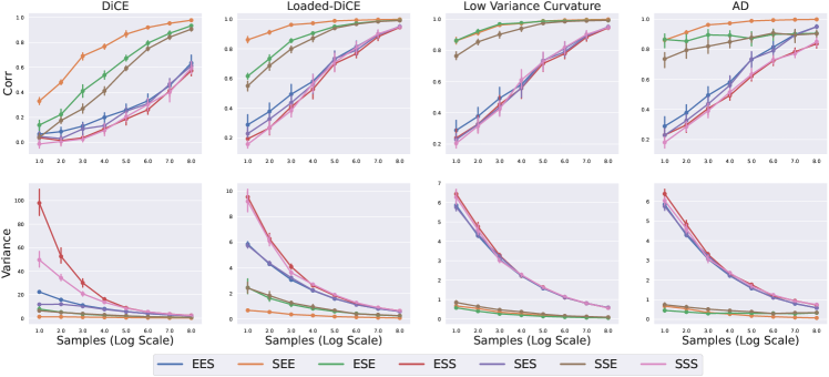
Figure 5: Ablation study on sample size and estimator in 1-step inner-loop setting. (1) Outer-loop policy gradient is important for estimation (2) Compositional bias correction helps increase the correlation (3) The LVC and Loaded-DiCE can achieve higher correlation compared with AD when the Hessian matrix is estimated.

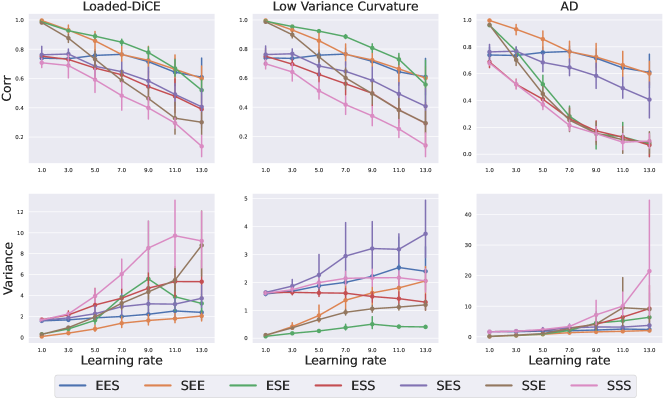
Figure 6: Ablation study on inner learning rate and estimator. (1) In Loaded-DiCE and LVC, With larger learning rate, the compositional bias basically shares the same importance with Hessian estimation error. (2) With larger learning rate, the Hessian estimation problem in AD largely decreases the correlation.

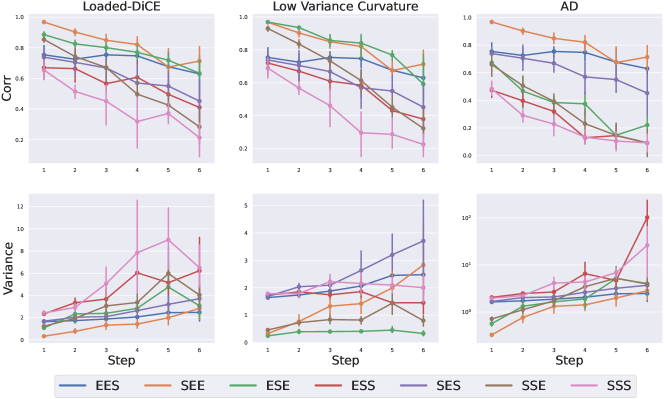
Figure 7: Ablation study on inner step and estimator. Results of larger steps show similar phenomenon with larger inner-loop learning rate.

I.1.4 Additional Experimental Results on Tabular LIRPG

In Fig. 8 we offer additional experimental Results on estimation variance. Basically the AD based estimation in LIRPG setting tend to have higher variance.

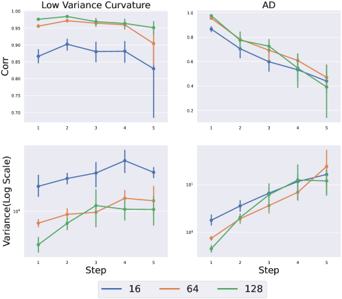
Figure 8: Additional experiment results on. Different color refers to different trajectory sample size.

I.1.5 Hyperparameters

We offer the hyperparameter settings for our Tabular MDP experiment in Table 2.

Table 2: Hyper-parameter settings for Tabular MDP.

Settings	Value	Description
Trajectory length	20	RL trajecotry length
Discount factor	0.8	Learning rate for meta-solver updates
Inner learning rate	10	Learning rate for inner-loop update
Inner step	1	step number of inner-update
Independent trials	10	Number of independent trials on environments
Same trials	20	number of independent trials on the same point
Dimension of state	20	dimension of state
Dimension of action	5	Dimension of action
Noise coefficient	1.0	Noise factor for simulating estimated value function
Density	0.001	Parameters of Dirichilet Distribution

I.2 LOLA-DiCE on Iterated Prisoner Dilemma (IPD)

I.2.1 Experimental Settings

In Iterated Prisoner Dilemma, the Prisoner Dilemma game is played repeatedly by the same players. The payoffs of Prisoner Dilemma for players are shown as follows.

$$\mathbf{R}^{1}=\left[\begin{matrix}-2&0\\ -3&-1\end{matrix}\right]\quad\mathbf{R}^{2}=\left[\begin{matrix}-2&-3\\ 0&-1\end{matrix}\right],$$

where the action 0 (correpsonds to column/row 0) as "cooperation" (don’t confess) and the action 1 (correpsonds to column/row 1) as "defection" (confess). Agent in Iterated Prisoner Dilemma aims at maximising the cumulative Discounted reward. By LOLA-DiCE algorithm, it is possible for both agent to reach social welfare: (-1, -1). Refer to Appendix A.2 for how the algorithm is formulated.

We conduct our experiment by adapting code from the official codebase. The official code only conducts the experiment using one fixed seed and the performance is highly sensitive to different random seeds using default hyperparameters. To evaluate the performance reliably, we conduct all the experiments for 10 random seeds and report the average result.

I.2.2 Additional Experimental Results

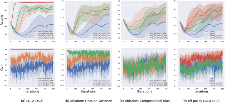
Figure 9: Experiment result of LOLA-DiCE. (a) Poor inner-loop estimation can fail the LOLA-DiCE algorithm. (b) Hessian estimation variance is the main problem in LOLA-DiCE. (c) The correction of compositional bias also helps increase the average return. (d) The off-policy correction can both decrease the compositional bias and Hessian estimation variance, which largely increases the final return.

Ablation on LOLA-DiCE inner/outer estimation. We report the correlation result of conducting ablation study for different inner/outer-loop estimation of LOLA-DiCE in the Fig. 9(a). Higher correlation does not guarantee higher return. The bonus brought by setting inner-loop as exact solution have a really large improvement over correlation (from 0.7 to 1.0) but have limited improvement on return. We believe it is because the outer-loop gradient estimation becomes the main issue when inner-loop estimation is really well.

Ablation on LOLA-DiCE Hessian variance and compositional bias. We show additional experimental result in Fig. 9(c). An interesting thing is that we find out the gradient correlation of these three settings are comparable. An possible explanation is that the main issue here is the hessian variance and this is why the performance gain by lowering hessian variance is larger that lowering compositional bias. Though by correcting compositional bias LOLA can have better estimation with performance gain, the gain is not obvious in the aspect of gradient correlation because the hessian variance is still large.

Off-policy DiCE and ablation study The correlation gain for off-policy comp$\&$on-policy hessian is still limited like that in Fig. 9(c). But the performance gain verifies the bonus brought by correcting compositional bias.

I.2.3 Hyperparameters

We offer the hyperparameter settings for our LOLA experiment in Table 3.

Table 3: Hyper-parameter settings for LOLA-DiCE.

Settings	Value	Description
Outer Learning rate	0.1	Outer Learning rate
Inner Learning rate	0.3	Inner Learning rate
Discount factor	0.96	Discount factor
Update	500	step number of meta-update
Rollout Length	100	Length of IPD rollout
Inner step	1	number of virtual inner-step look-ahead
Value function learning rate	0.1	Value function learning rate
Off-policy buffer size	1024	Buffer size
Sample batch size	128	Comp/Hessian/Outer sample batch size

I.3 MGRL on Atari games

I.3.1 Experimental setting

We reimplement the MGRL algorithm based on A2C baseline. In this case, Meta-parameters $\phi$ involves 4 hyperparameters: Discount factor, value loss coefficient, entropy loss coefficient and GAE ratio. The procedures of ’discard’ strategy we use is summarized as follows: Starting from the inner-policy parameters $\theta^{0}$, we utilise take 3 A2C updates and get the 3-step updated policy $\theta^{3}$. Then we can calculate the meta-gradient by backpropogating from $R(\theta^{3})$ to the meta parameters. Finally we reset the inner-loop policy parameters back to $\theta^{1}$ so the rest 2 updates are in fact virtual update. It is only used for the meta-gradient estimation.

I.3.2 Discussion on the ’Discard’ strategy

In the MGRL experiment, we follow previous work [4] for conducting multi-step MGRL. So the inner-loop policy will take multi-step virtual updates for meta-parameters update. As mentioned in Section 4.2 in their paper, this strategy can only keep the RL update times unchanged among different algorithms and is not particularly sample efficient because they need to take virtual look-ahead for the update of meta-parameters. However, one benefit of adopting such strategy is that we can keep the amount of meta-update large enough to verify the effect brought by the LVC correction. We also take some experiments on another setting where we take meta-update after each 3-step inner-loop update. Note that they are no longer virtual inner-loop updates. However, we find out that in many environment this setting largely decrease the meta-update times and make the comparison of different meta-gradient estimation less meaningful.

I.3.3 Additional Experimental results

We offer the full experiments results on all 8 Atari games: Asteroids, Qbert, Tennis, BeamRider, Alien, Assault, DoubleDunk, Seaquest. The reward performance is shown in Fig. 10. We also offer trajectories for all 4 meta-parameters on these experiments in Fig. 11. From Fig. 10 it can show that MGRL with LVC correction can achieve comparable or better performance in almost all 8 environments. Note that we need to clarify that in some RL experiments the MGRL cannot achieve better performance compared with A2C baseline. This also corresponds to the experimental results in original MGRL paper [39]. However, since our main comparison only happens between MGRL and MGRL with LVC correction, it is still a fair comparison to verify the effectiveness of LVC hessian correction. Fig. 11 reveals that even we have only 4 meta-parameters, different meta-gradient estimation can still results in large gap between the meta optimisation trajectory and final GMRL performance.

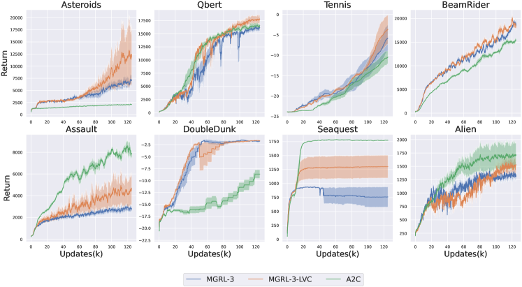
Figure 10: Experimental results on Atari game over 5 seeds. 3-step MGRL with LVC correction can achieve at least the same performance compared with 3-step MGRL in basically all environments.

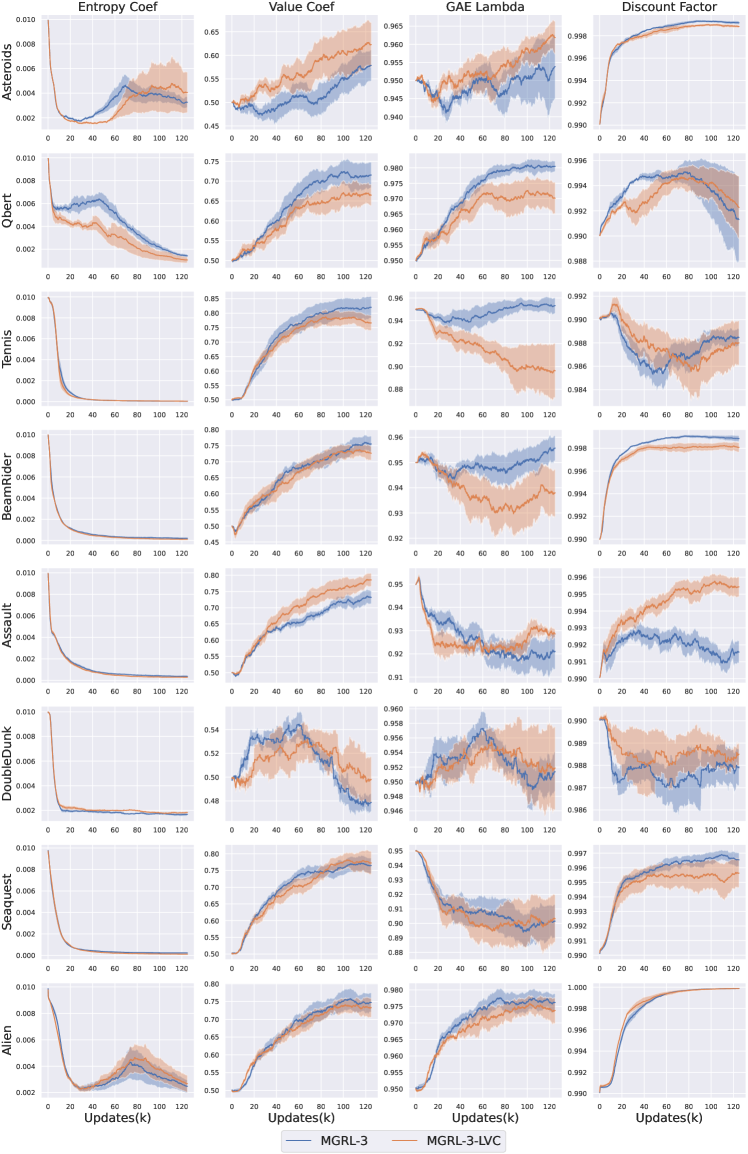
Figure 11: 4 Meta parameters trajectories on Atari game for 3-step MGRL and 3-step MGRL with LVC correction.

I.3.4 Implementations and hyperparameters

We adopt the codebase of A2C from [21] and differentiable optimization library [28] to implement MGRL algorithms. We use a shared CNN network (3 Conv layers and one fully connected (FC) layer) for the policy network and critic network. The (out-channel, filters, stride) for each Conv layer is (32, $8\times 8$, 4), (64, $4\times 4$, 2) and (64, $3\times 3$, 1) respectively while the hidden size is 512 for the FC layer. For the training loss, we adopt additional entropy regularisation for policy loss and Mean Square Error (MSE) for the value loss. We adopt the Generalized Advantage estimation (GAE) for advantage estimation. We offer the hyperparameter settings for our experiment in Table 4. We tun our algorithm for 125k inner updates, which corresponds to 40M environment steps for baseline A2C.

Table 4: Hyper-parameter settings for MGRL.

Settings	Value	Description
Inner Learning rate	7e-4	Inner Learning rate
Learning rate Scheduling	Linear decay	linearly decrease to 0
Discount factor	0.99	Discount factor
GAE LAMBDA	0.95	ratio of generalized advantage estimation
Value coef	0.5	coefficient of value loss
entropy coef	0.01	coefficient of entropy loss
Update	125k	number of inner update
Number of process	64	number of multi process
number of step per update	5	number of step per update
Meta update	3	number of inner-update for conducting meta-update
Meta learning rate	0.001	meta learning rate
Inner optimizer	Adam	Inner-loop optimizer
Outer optimizer	Adam	Outer-loop optimizer

Appendix J Author contribution

We summarise the main contributions from each of the authors as follows:

Bo Liu: Algorithm design, main theoretical proof, some code implementation and experiments running (on tabular MDP and MGRL), and paper writing.

Xidong Feng: Idea proposing, algorithm design, part of theoretical proof, main code implementation and experiments running (on tabular MDP, LOLA and MGRL), and paper writing.

Jie Ren: Code implementation and experiments running for MGRL.

Luo Mai: Project discussion and paper writing.

Rui Zhu: Project discussion and paper writing.

Jun Wang: Project discussion and overall project supervision.

Yaodong Yang: Project lead, idea proposing, experiment supervision, and whole manuscript writing.

References

- Al-Shedivat et al. [2017] Maruan Al-Shedivat, Trapit Bansal, Yuri Burda, Ilya Sutskever, Igor Mordatch, and Pieter Abbeel. Continuous adaptation via meta-learning in nonstationary and competitive environments. arXiv preprint arXiv:1710.03641, 2017.
- Baydin et al. [2017] Atilim Gunes Baydin, Robert Cornish, David Martinez Rubio, Mark Schmidt, and Frank Wood. Online learning rate adaptation with hypergradient descent. arXiv preprint arXiv:1703.04782, 2017.
- Bechtle et al. [2021] Sarah Bechtle, Artem Molchanov, Yevgen Chebotar, Edward Grefenstette, Ludovic Righetti, Gaurav Sukhatme, and Franziska Meier. Meta learning via learned loss. In 2020 25th International Conference on Pattern Recognition (ICPR), pages 4161–4168. IEEE, 2021.
- Bonnet et al. [2021] Clément Bonnet, Paul Caron, Thomas Barrett, Ian Davies, and Alexandre Laterre. One step at a time: Pros and cons of multi-step meta-gradient reinforcement learning. arXiv preprint arXiv:2111.00206, 2021.
- Duan et al. [2016] Yan Duan, John Schulman, Xi Chen, Peter L Bartlett, Ilya Sutskever, and Pieter Abbeel. Rl: Fast reinforcement learning via slow reinforcement learning. arXiv preprint arXiv:1611.02779, 2016.
- Fallah et al. [2020] Alireza Fallah, Aryan Mokhtari, and Asuman Ozdaglar. On the convergence theory of gradient-based model-agnostic meta-learning algorithms. In International Conference on Artificial Intelligence and Statistics, pages 1082–1092. PMLR, 2020.
- Fallah et al. [2021] Alireza Fallah, Kristian Georgiev, Aryan Mokhtari, and Asuman Ozdaglar. On the convergence theory of debiased model-agnostic meta-reinforcement learning. Advances in Neural Information Processing Systems, 34:3096–3107, 2021.
- Farquhar et al. [2019] Gregory Farquhar, Shimon Whiteson, and Jakob Foerster. Loaded dice: trading off bias and variance in any-order score function estimators for reinforcement learning. arXiv preprint arXiv:1909.10549, 2019.
- Feng et al. [2021] Xidong Feng, Oliver Slumbers, Ziyu Wan, Bo Liu, Stephen McAleer, Ying Wen, Jun Wang, and Yaodong Yang. Neural auto-curricula in two-player zero-sum games. Advances in Neural Information Processing Systems, 34, 2021.
- Finn et al. [2017] Chelsea Finn, Pieter Abbeel, and Sergey Levine. Model-agnostic meta-learning for fast adaptation of deep networks. In International Conference on Machine Learning, pages 1126–1135. PMLR, 2017.
- Foerster et al. [2018a] Jakob Foerster, Richard Y Chen, Maruan Al-Shedivat, Shimon Whiteson, Pieter Abbeel, and Igor Mordatch. Learning with opponent-learning awareness. In Proceedings of the 17th International Conference on Autonomous Agents and MultiAgent Systems, pages 122–130, 2018a.
- Foerster et al. [2018b] Jakob Foerster, Gregory Farquhar, Maruan Al-Shedivat, Tim Rocktäschel, Eric Xing, and Shimon Whiteson. Dice: The infinitely differentiable monte carlo estimator. In International Conference on Machine Learning, pages 1529–1538. PMLR, 2018b.
- Foerster et al. [2017] Jakob N Foerster, Richard Y Chen, Maruan Al-Shedivat, Shimon Whiteson, Pieter Abbeel, and Igor Mordatch. Learning with opponent-learning awareness. arXiv preprint arXiv:1709.04326, 2017.
- Franceschi et al. [2017] Luca Franceschi, Michele Donini, Paolo Frasconi, and Massimiliano Pontil. Forward and reverse gradient-based hyperparameter optimization. In International Conference on Machine Learning, pages 1165–1173. PMLR, 2017.
- Fu et al. [2020] Haotian Fu, Hongyao Tang, Jianye Hao, Chen Chen, Xidong Feng, Dong Li, and Wulong Liu. Towards effective context for meta-reinforcement learning: an approach based on contrastive learning. arXiv preprint arXiv:2009.13891, 2020.
- Gupta et al. [2018] Abhishek Gupta, Russell Mendonca, YuXuan Liu, Pieter Abbeel, and Sergey Levine. Meta-reinforcement learning of structured exploration strategies. Advances in Neural Information Processing Systems, 31:5302–5311, 2018.
- Hu et al. [2020] Yujing Hu, Weixun Wang, Hangtian Jia, Yixiang Wang, Yingfeng Chen, Jianye Hao, Feng Wu, and Changjie Fan. Learning to utilize shaping rewards: A new approach of reward shaping. Advances in Neural Information Processing Systems, 33, 2020.
- Ji et al. [2020] Kaiyi Ji, Junjie Yang, and Yingbin Liang. Multi-step model-agnostic meta-learning: Convergence and improved algorithms. CoRR, abs/2002.07836, 2020.
- Kim et al. [2020] Dong-Ki Kim, Miao Liu, Matthew Riemer, Chuangchuang Sun, Marwa Abdulhai, Golnaz Habibi, Sebastian Lopez-Cot, Gerald Tesauro, and Jonathan P How. A policy gradient algorithm for learning to learn in multiagent reinforcement learning. arXiv preprint arXiv:2011.00382, 2020.
- Kirsch et al. [2019] Louis Kirsch, Sjoerd van Steenkiste, and Juergen Schmidhuber. Improving generalization in meta reinforcement learning using learned objectives. In International Conference on Learning Representations, 2019.
- Kostrikov [2018] Ilya Kostrikov. Pytorch implementations of reinforcement learning algorithms. https://github.com/ikostrikov/pytorch-a2c-ppo-acktr-gail, 2018.
- Letcher et al. [2018] Alistair Letcher, Jakob Foerster, David Balduzzi, Tim Rocktäschel, and Shimon Whiteson. Stable opponent shaping in differentiable games. In International Conference on Learning Representations, 2018.
- Liu et al. [2019] Hao Liu, Richard Socher, and Caiming Xiong. Taming maml: Efficient unbiased meta-reinforcement learning. In International Conference on Machine Learning, pages 4061–4071. PMLR, 2019.
- Mao et al. [2019] Jingkai Mao, Jakob Foerster, Tim Rocktäschel, Maruan Al-Shedivat, Gregory Farquhar, and Shimon Whiteson. A baseline for any order gradient estimation in stochastic computation graphs. In International Conference on Machine Learning, pages 4343–4351. PMLR, 2019.
- Mnih et al. [2016] Volodymyr Mnih, Adria Puigdomenech Badia, Mehdi Mirza, Alex Graves, Timothy Lillicrap, Tim Harley, David Silver, and Koray Kavukcuoglu. Asynchronous methods for deep reinforcement learning. In International conference on machine learning, pages 1928–1937. PMLR, 2016.
- Oh et al. [2020] Junhyuk Oh, Matteo Hessel, Wojciech M Czarnecki, Zhongwen Xu, Hado van Hasselt, Satinder Singh, and David Silver. Discovering reinforcement learning algorithms. arXiv preprint arXiv:2007.08794, 2020.
- Rakelly et al. [2019] Kate Rakelly, Aurick Zhou, Chelsea Finn, Sergey Levine, and Deirdre Quillen. Efficient off-policy meta-reinforcement learning via probabilistic context variables. In International conference on machine learning, pages 5331–5340. PMLR, 2019.
- Ren et al. [2022] Jie Ren, Xidong Feng, Bo Liu, Xuehai Pan, Luo Mai, and Yaodong Yang. Torchopt. https://github.com/metaopt/torchopt, 2022.
- Rothfuss et al. [2019] Jonas Rothfuss, Dennis Lee, Ignasi Clavera, Tamim Asfour, and Pieter Abbeel. Promp: Proximal meta-policy search. In 7th International Conference on Learning Representations, ICLR 2019, New Orleans, LA, USA, May 6-9, 2019. OpenReview.net, 2019.
- Schmidhuber [1987] Jürgen Schmidhuber. Evolutionary principles in self-referential learning, or on learning how to learn: the meta-meta-… hook. PhD thesis, Technische Universität München, 1987.
- Shapley [1953] Lloyd S Shapley. Stochastic games. Proceedings of the national academy of sciences, 39(10):1095–1100, 1953.
- Sutton and Barto [2018] Richard S Sutton and Andrew G Barto. Reinforcement learning: An introduction. MIT press, 2018.
- Tang et al. [2021] Yunhao Tang, Tadashi Kozuno, Mark Rowland, Remi Munos, and Michal Valko. Unifying gradient estimators for meta-reinforcement learning via off-policy evaluation. Advances in Neural Information Processing Systems, 34, 2021.
- Veeriah et al. [2019] Vivek Veeriah, Matteo Hessel, Zhongwen Xu, Richard Lewis, Janarthanan Rajendran, Junhyuk Oh, Hado van Hasselt, David Silver, and Satinder Singh. Discovery of useful questions as auxiliary tasks. arXiv preprint arXiv:1909.04607, 2019.
- Veeriah et al. [2021] Vivek Veeriah, Tom Zahavy, Matteo Hessel, Zhongwen Xu, Junhyuk Oh, Iurii Kemaev, Hado van Hasselt, David Silver, and Satinder Singh. Discovery of options via meta-learned subgoals. arXiv preprint arXiv:2102.06741, 2021.
- Vuorio et al. [2021] Risto Vuorio, Jacob Austin Beck, Gregory Farquhar, Jakob Nicolaus Foerster, and Shimon Whiteson. No DICE: An investigation of the bias-variance tradeoff in meta-gradients. In Deep RL Workshop NeurIPS 2021, 2021.
- Wang et al. [2016] Jane X Wang, Zeb Kurth-Nelson, Dhruva Tirumala, Hubert Soyer, Joel Z Leibo, Remi Munos, Charles Blundell, Dharshan Kumaran, and Matt Botvinick. Learning to reinforcement learn. arXiv preprint arXiv:1611.05763, 2016.
- Williams [1992] Ronald J Williams. Simple statistical gradient-following algorithms for connectionist reinforcement learning. Machine learning, 8(3-4):229–256, 1992.
- Xu et al. [2018] Zhongwen Xu, Hado van Hasselt, and David Silver. Meta-gradient reinforcement learning. arXiv preprint arXiv:1805.09801, 2018.
- Xu et al. [2020] Zhongwen Xu, Hado van Hasselt, Matteo Hessel, Junhyuk Oh, Satinder Singh, and David Silver. Meta-gradient reinforcement learning with an objective discovered online. arXiv preprint arXiv:2007.08433, 2020.
- Zahavy et al. [2020] Tom Zahavy, Zhongwen Xu, Vivek Veeriah, Matteo Hessel, Junhyuk Oh, Hado van Hasselt, David Silver, and Satinder Singh. A self-tuning actor-critic algorithm. arXiv preprint arXiv:2002.12928, 2020.
- Zheng et al. [2018] Zeyu Zheng, Junhyuk Oh, and Satinder Singh. On learning intrinsic rewards for policy gradient methods. Advances in Neural Information Processing Systems, 31:4644–4654, 2018.
- Zheng et al. [2020] Zeyu Zheng, Junhyuk Oh, Matteo Hessel, Zhongwen Xu, Manuel Kroiss, Hado Van Hasselt, David Silver, and Satinder Singh. What can learned intrinsic rewards capture? In International Conference on Machine Learning, pages 11436–11446. PMLR, 2020.
- Zhou et al. [2020] Wei Zhou, Yiying Li, Yongxin Yang, Huaimin Wang, and Timothy Hospedales. Online meta-critic learning for off-policy actor-critic methods. Advances in Neural Information Processing Systems, 33, 2020.