A new phase in the Lorentzian type IIB matrix model and the emergence of continuous space-time

Abstract

The Lorentzian type IIB matrix model is a promising candidate for a non-perturbative formulation of superstring theory. In previous studies, Monte Carlo calculations provided interesting results indicating the spontaneous breaking of SO(9) to SO(3) and the emergence of (3+1)-dimensional space-time. However, an approximation was used to avoid the sign problem, which seemed to make the space-time structure singular. In this talk, we report our results obtained by using the complex Langevin method to overcome the sign problem instead of using this approximation. In particular, we discuss the emergence of continuous space-time in a new phase, which we discovered recently.

1 Introduction

Superstring theory is the most promising candidate for a unified theory of all interactions, including gravity. The theory is consistently defined in ten-dimensional space-time, and the extra six dimensions need to be small enough to be consistent with current observations. One mechanism that leads to phenomenologically acceptable scenarios is the compactification of the extra dimensions into small compact internal spaces. These scenarios have been investigated perturbatively on D-brane backgrounds and result in a vast number of vacua, leading to the so-called string landscape. It is therefore interesting to see what happens when one includes nonperturbative effects and whether these play an essential role in determining the true vacuum of the theory.

In 1996, the type IIB, or IKKT, matrix model was proposed as a nonperturbative formulation of superstring theory [1]. The model is obtained by dimensionally reducing the action of the ten-dimensional ${\cal N}=1$ Super Yang-Mills (SYM) to zero dimensions. The resulting matrix model has maximal ${\cal N}=2$ supersymmetry (SUSY) and the translations of the SUSY algebra is realized by the shifts $A_{\mu}\to A_{\mu}+\alpha_{\mu}\mathbf{1}$, $\mu=0,\ldots,9$. The eigenvalues of the bosonic matrices $A_{\mu}$ are considered to define space-time; therefore, although space-time does not exist a priori in the model, it emerges from the dynamics of the theory. The model has the potential to provide a nonperturbative mechanism for dynamical compactification of the extra dimensions in superstring theory. Such a scenario has been shown to be realized in the model’s Euclidean version. In this case, dynamical compactification is realized by the Spontaneous Symmetry Breaking (SSB) of the SO(10) rotational symmetry down to SO(3), resulting in a three-dimensional macroscopic universe. This was shown by applying the Gaussian Expansion Method (GEM) [2, 3, 4, 5], which is a systematic expansion yielding nonperturbative information, and by Monte Carlo calculations [6, 7, 8, 9].

Those results provide a strong motivation to study the model in its original, Lorentzian version. A straightforward Monte Carlo calculation is not possible because the model has a strong complex action problem. This led the authors in [10] to use an approximation that completely removes the complex action problem. They found that the model features a dynamically emerging continuous time, and that space is expanding from Planck scale to a macroscopic three dimensional universe. This happens by SSB the SO(9) rotational symmetry of space down to SO(3). Following works showed that this expansion has the potential to be phenomenologically viable, being exponential at short times and power like at late times [11, 12, 13, 14]. At late times, the dominant configurations can be approximated by classical solutions representing an expanding space that contain phenomenologically consistent matter content at low energies [15, 16, 17, 18, 19, 20, 21, 22, 23, 24, 25, 26, 27].

Recent work shows that the expansion is driven by singular configurations associated with the Pauli matrices, in which only two eigenvalues are large [28]. This behavior is due to the approximation used to avoid the complex action problem; therefore it becomes necessary to perform calculations in the full Lorentzian model. In that case, the partition function is not well defined, and in [29] it was proposed to perform two independent world-sheet and target space Wick rotations, parameterized by two parameters $s$ and $k$, respectively, and then take an appropriate $s,k\to 0$ limit. Even after this deformation, the model suffers from a severe complex action problem, which the authors overcame by using the Complex Langevin Method (CLM) [30, 31]. The CLM has been known to yield wrong results in many interesting cases, but by applying new techniques, and correct convergence criteria [32, 33, 34, 35, 36, 37, 38], it is possible to use the method successfully. Recently, the CLM has been applied to the Euclidean IIB matrix model, yielding results that are in agreement with GEM calculations [8, 9].

This work applies the CLM to a simplified version of the IIB matrix model, where the fermionic degrees of freedom are quenched (bosonic IIB). The model is deformed by the Wick rotations mentioned above, and we are able to study $(s,k)$ deformations for $k=0$, $-1\leq s\leq 0$. The $s=-1$ model is the one studied in [10] and the $s=0$ model is the bosonic Lorentzian IIB matrix model. The simulations are successful, and we observe a transition from the singular “Pauli Matrix” dominated phase to a new, continuous phase. We observe that the dominant configurations are continuous, non-expanding space-times. As in the case of the Euclidean model, we expect that SUSY plays an essential role in the SSB of the rotational symmetry of space. We expect to report results in this direction in future work.

2 The Model

The Lorentzian type IIB matrix model is given by

$$Z=\int\mathcal{D}A\mathcal{D}\Psi e^{-S(A,\Psi)},$$ (1)

$$S(A,\Psi)=iN\beta\left\{\frac{1}{4}{\rm Tr}\left[A_{\mu},A_{\nu}\right]^{2}+\frac{1}{2}{\rm Tr}\left(\Psi_{\alpha}(\mathcal{C}\Gamma^{\mu})_{\alpha\beta}\left[A_{\mu},\Psi_{\beta}\right]\right)\right\},$$ (2)

where $A_{\mu}$ and $\Psi_{\alpha}$ are $N\times N$ Hermitian matrices. $\Gamma^{\mu}$ and $\mathcal{C}$ are 10–dimensional gamma matrices and the charge conjugation matrix, respectively, which are obtained after the Weyl projection. The index $\mu$ runs from $0$ to $9$, and $\alpha$ runs from $1$ to $16$. This model has an SO(9,1) Lorentz symmetry, under which $A_{\mu}$ and $\Psi_{\alpha}$ transform as a 10-dimensional Lorentz vector and a Majorana-Weyl spinor, respectively. Since the numerical cost for the evaluation of the fermionic part is very high, we neglect the fermionic contribution hereafter. Namely, we omit the second term of eq. (2).

We consider the world-sheet and target space Wick rotations proposed in [29], parameterized by the real parameters $(s,k)$

$$Z=\int\mathcal{D}Ae^{-\bar{S}_{\rm b}(A)},$$ (3)

$$\bar{S}_{\rm b}(A)=-iN\beta e^{is\pi/2}\left\{\frac{1}{2}e^{-ik\pi}{\rm Tr}\left[A_{0},A_{i}\right]^{2}-\frac{1}{4}{\rm Tr}\left[A_{i},A_{j}\right]^{2}\right\}.$$ (4)

The values of $(s,k)$ must be such that the real part of $\bar{S}_{\rm b}(A)$ is positive. When $(s,k)=(0,0)$ we have the Lorentzian bosonic version of the IIB matrix model, whereas when $(s,k)=(1,1)$ we obtain the Euclidean bosonic version of the IIB matrix model. For simplicity, we refer to those models as the “Lorentzian” and the “Euclidean” models. The case $(s,k)=(-1,0)$ corresponds to the model first studied in [10]. Therefore, the model defined in (4) interpolates continuously between these three cases.

We also introduce the IR constraints

$$\frac{1}{N}{\rm Tr}\left(A_{0}\right)^{2}=\kappa\,,\qquad\frac{1}{N}{\rm Tr}\left(A_{i}\right)^{2}=1\,,$$ (5)

in order to reduce the fluctuations of the zero modes in eq. (3).

One of the non-trivial features of the model is the emergence of continuous time from its dynamics. If we choose the SU($N$) basis which diagonalizes the $A_{0}$ such that

$$\begin{split}A_{0}={\rm diag}\left(\alpha_{1},\alpha_{2},...,\alpha_{N}\right)\,,\qquad\alpha_{1}\leq\alpha_{2}\leq\cdots\leq\alpha_{N},\end{split}$$ (6)

then, in the model studied in [10], the spatial matrices exhibit a band-diagonal structure, where $|(A_{i})_{\nu+p,\nu+q}|\ll 1$ for $p^{2}+q^{2}<n^{2}$. We call $n$ the band width, and we define the $n\times n$ block matrices

$$\left(\bar{A_{i}}\right)_{ab}(t)=\left(A_{i}\right)_{\nu+a,\nu+b},$$ (7)

where $t$ is defined by

$$t=\sum_{a=1}^{n}\left(A_{0}\right)_{\nu+a,\nu+a}=\sum_{a=1}^{n}\alpha_{\nu+a}.$$ (8)

It is natural to consider that the matrices $\bar{A}_{i}(t)$ represent (fuzzy) space at time $t$.

3 The Complex Langevin Method

The complex Langevin method (CLM) was introduced by Klauder and Parisi independently as one of the methods to overcome the notorious sign problem [30, 31]. The idea of the CLM is complexifying the dynamical variable to evaluate the complex Boltzmann weight correctly. In this section, we briefly explain the CLM.

Consider the case of a complex-valued action $S(x)\in\mathbb{C}$ with a set of real-valued dynamical variables $x\in\mathbb{R}^{n}$. The partition function is given by

$$Z=\int dx\ e^{-S(x)}.$$ (9)

Since $e^{-S(x)}$ is complex, in most interesting cases, the usual Monte Carlo methods are not applicable. In the CLM, we complexify the dynamical variables as

$$x\in\mathbb{R}^{n}\to z\in\mathbb{C}^{n}.$$ (10)

Then the partition function is given by

$$Z=\int dz\ e^{-S(z)},$$ (11)

and the complex Langevin equation is obtained as

$$\frac{dz_{i}}{dt_{\rm L}}=-\frac{\partial S}{\partial z_{i}}+\eta_{i}(t_{\rm L}),$$ (12)

where $t_{\rm L}$ is the (fictitious) Langevin time, the $\eta_{i}(t_{\rm L})$ can be chosen to be real Gaussian noise, which satisfies

$$\Braket{\eta_{i}(t_{\rm L})\eta_{j}(t_{\rm L}^{\prime})}_{\eta}=2\delta_{i,j}\delta_{t_{\rm L},t_{\rm L}^{\prime}},$$ (13)

and $\frac{\partial S(z)}{\partial z_{i}}$ is the drift term. The drift term $\frac{\partial S(z)}{\partial z_{i}}$ is obtained from $\frac{\partial S(x)}{\partial x_{i}}$ by analytic continuation.

It is known that the CLM might yield wrong results. Fortunately, a criterion for the solutions of (12) to give the expectation values of the model defined by the partition function (9) was proposed quite recently [33, 37]. The criterion is that the distribution of the drift term values should be suppressed exponentially or faster for a large magnitude of its values. The assumption of holomorphicity is crucial for the correctness of the method.

The first step is to make a change of variables to realize the order of the eigenvalues of $A_{0}$ [29]. We introduce new variables $\tau_{i}$ as

$$\alpha_{a}=\sum_{i=1}^{a-1}e^{\tau_{i}},$$ (14)

and we treat the $\tau_{i}$ as the dynamical variables, which are complexified in the CLM. Then the order (6) is automatically realized.

Next we apply the CLM to the model. The complex Langevin equation is the following:

$$\begin{split}\frac{d\tau_{a}}{dt_{\rm L}}&=-\frac{\partial\bar{S}_{\rm eff}}{\partial\tau_{a}}+\eta_{a}(t_{\rm L}),\\ \frac{d(A_{i})_{ab}}{dt_{\rm L}}&=-\frac{\partial\bar{S}_{\rm eff}}{\partial(A_{i})_{ba}}+(\eta_{i})_{ab}(t_{\rm L}),\end{split}$$ (15)

where $t_{\rm L}$ is the Langevin time, and $\eta$ is the Gaussian noise. The matrices $(\eta_{i})_{ab}(t_{\rm L})$ are chosen to be Hermitian. The effective action $\bar{S}_{\rm eff}$ is obtained from $\bar{S}_{\rm b}$, by adding the appropriate gauge fixing and change of variable terms, as well as terms that enforce the constraints (5). In the original model, the drift terms $\frac{\partial\bar{S}_{\rm eff}}{\partial\tau_{a}}$ and $\frac{\partial\bar{S}_{\rm eff}}{\partial(A_{i})_{ba}}$ are defined for real variables $\tau_{a}$ and Hermitian matrices $(A_{i})_{ba}$. In the CLM, we perform an analytic continuation by taking complex ${\tau_{a}}$ and general complex matrices $(A_{i})_{ba}$.

4 Results

First we show the result for $(s,k)=(-1,0)$ case, which corresponds to the approximation used in [16, 28]. Then we try to approach $(s,k)=(0,0)$, which corresponds to the Lorentzian model.

4.1 $(s,k)=(-1,0)$ case

In order to study the SSB of the the SO(9) spatial symmetry, we define “the moment of inertia tensor" as

$$T_{ij}(t)\equiv{\rm tr}\left(\bar{X}_{i}(t)\bar{X}_{j}(t)\right),$$ (16)

where $\bar{X}_{i}(t)$ is defined as

$$\bar{X}_{i}(t)=\frac{1}{2}\left(\bar{A}_{i}(t)+\bar{A}^{\dagger}_{i}(t)\right),$$ (17)

and “${\rm tr}$" means the trace over the block matrices. When the space is SO(9) symmetric, the 9 eigenvalues have the same large–$N$ limit. In Figure 1 (Left), we plot the eigenvalues of $T_{ij}(t)$ against time $t$. At early times, the 9 eigenvalues are almost the same. On the other hand, 3 out of 9 eigenvalues start to grow at some time. This behavior indicates that SO(9) symmetry is spontaneously broken at this time, and a macroscopic SO(3) symmetric space emerges.

Next, to study the structure of the space, we define $Q(t)$ as

$$Q(t)\equiv\sum_{i=1}^{9}\left(\bar{X}_{i}(t)\right)^{2},$$ (18)

whose eigenvalues describe how space spreads into the radial direction. If the space is smooth, the spectrum of the eigenvalues is continuous. In Figure 1 (Right), we plot the eigenvalues of $Q(t)$ against time $t$. Only 2 eigenvalues start to grow at some point, which corresponds to when the SO(3) symmetric space starts to expand. This behavior means that the expansion of space is realized by only two isolated points at large distance. Therefore, space is not continuous [28].

Figure 1: Results for the bosonic model with $(s,k)=(-1,0),\ N=128,\ \beta=8.0,\ \kappa=0.04$. (Left) The eigenvalues of $T_{ij}(t)$ against time $t$. We find that only 3 out of 9 eigenvalues grow as time increases. (Right) The eigenvalues of $Q(t)$ against time $(t)$. Only 2 eigenvalues grow as time increases.

4.2 approaching $(s,k)=(0,0)$

We try to approach $(s,k)=(0,0)$ by using the CLM. We fix $k=0$ and do the simulations for various values of $s$. In Figure 2, we plot results for 3 different values of $s$. The (Left), (Center), and (Right) plots correspond to $s=-0.8,\ -0.6,\ {\rm and}\ 0$ respectively. The expansion behavior changes as $s$ approaches $0$. When $s\approx-0.8$, a bell-shaped expansion appears. If $s$ gets closer to $0$, at some point the expansion disappears ($s\approx-0.6$), and finally a parabola-shaped expansion appears at $s=0$. This parabola-shaped expansion is consistent with typical classical solutions [26].

In Figure 3, we plot the eigenvalues of $T_{ij}(t)$ against time $t$ for the $(s,k)=(0,0)$ case. We observe that the 9 eigenvalues do not indicate an SSB pattern, even at late times. Therefore the SSB of SO(9) does not occur in this case.

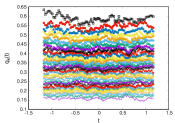
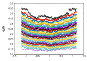
Figure 2: The eigenvalues of $Q(t)$ are plotted against time $t$. (Left) The $(s,k)=(-0.8,0)$ case. (Center) The $(s,k)=(-0.6,0)$ case. (Right) The $(s,k)=(0,0)$ case. The other parameters are common, namely $N=128,\ \beta=2.5,\ \kappa=0.8$.

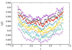
Figure 3: Result for $(s,k)=(0,0),\ N=128,\ \beta=2.5,$ and $\kappa=0.8$. The eigenvalues $\lambda_{i}(t)$ of $T_{ij}(t)$ are plotted against time $t$.

5 Summary and discussion

We applied the complex Langevin method (CLM) to the bosonic version of the type IIB matrix model to overcome the sign problem. As in [29], we introduced the two parameters $s$ and $k$, related to the Wick rotation on the world sheet and target space-time, respectively. The CLM was applied successfully, and we could simulate the model even at $s=k=0$. In this work, we explored the $k=0$, $-1\leq s\leq 0$ line, and we found a new phase in which the continuous space emerges as $s$ approaches $0$. In this phase, the expansion behavior changes and is consistent with the one found for the classical solutions obtained in [26]. However, the SSB of the SO(9) rotational symmetry is not observed.

In [39], we discuss the relation between the Lorentzian ($s=k=0$) and the Euclidean ($s=k=1$) case. We have found that the behavior at the new phase is equivalent to the behavior obtained in the Euclidean model. This paper also discusses possible scenarios for emergent Lorentzian space-time at late times.

It is known that supersymmetry plays a central role in realizing the SSB of the SO(10) to SO(3) rotational symmetry in the Euclidean model [9], and by neglecting the effects of the fermions, the SSB does not occur. Therefore, we expect that supersymmetry will play an essential role in realizing the SSB of the SO(9) symmetry, leading to an expanding space and a promising matrix model cosmology.

References

- [1] N. Ishibashi, H. Kawai, Y. Kitazawa and A. Tsuchiya, A Large N reduced model as superstring, Nucl. Phys. B 498 (1997) 467 [hep-th/9612115].
- [2] J. Nishimura and F. Sugino, Dynamical generation of four-dimensional space-time in the IIB matrix model, JHEP 05 (2002) 001 [hep-th/0111102].
- [3] H. Kawai, S. Kawamoto, T. Kuroki, T. Matsuo and S. Shinohara, Mean field approximation of IIB matrix model and emergence of four-dimensional space-time, Nucl. Phys. B 647 (2002) 153 [hep-th/0204240].
- [4] T. Aoyama and H. Kawai, Higher order terms of improved mean field approximation for IIB matrix model and emergence of four-dimensional space-time, Prog. Theor. Phys. 116 (2006) 405 [hep-th/0603146].
- [5] J. Nishimura, T. Okubo and F. Sugino, Systematic study of the SO(10) symmetry breaking vacua in the matrix model for type IIB superstrings, JHEP 10 (2011) 135 [1108.1293].
- [6] K.N. Anagnostopoulos, T. Azuma and J. Nishimura, Monte Carlo studies of the spontaneous rotational symmetry breaking in dimensionally reduced super Yang-Mills models, JHEP 11 (2013) 009 [1306.6135].
- [7] K.N. Anagnostopoulos, T. Azuma and J. Nishimura, Monte Carlo studies of dynamical compactification of extra dimensions in a model of nonperturbative string theory, PoS LATTICE2015 (2016) 307 [1509.05079].
- [8] K.N. Anagnostopoulos, T. Azuma, Y. Ito, J. Nishimura and S.K. Papadoudis, Complex Langevin analysis of the spontaneous symmetry breaking in dimensionally reduced super Yang-Mills models, JHEP 02 (2018) 151 [1712.07562].
- [9] K.N. Anagnostopoulos, T. Azuma, Y. Ito, J. Nishimura, T. Okubo and S. Kovalkov Papadoudis, Complex Langevin analysis of the spontaneous breaking of 10D rotational symmetry in the Euclidean IKKT matrix model, JHEP 06 (2020) 069 [2002.07410].
- [10] S.-W. Kim, J. Nishimura and A. Tsuchiya, Expanding (3+1)-dimensional universe from a Lorentzian matrix model for superstring theory in (9+1)-dimensions, Phys. Rev. Lett. 108 (2012) 011601 [1108.1540].
- [11] Y. Ito, S.-W. Kim, J. Nishimura and A. Tsuchiya, Monte Carlo studies on the expanding behavior of the early universe in the Lorentzian type IIB matrix model, PoS LATTICE2013 (2014) 341 [1311.5579].
- [12] Y. Ito, S.-W. Kim, Y. Koizuka, J. Nishimura and A. Tsuchiya, A renormalization group method for studying the early universe in the Lorentzian IIB matrix model, PTEP 2014 (2014) 083B01 [1312.5415].
- [13] Y. Ito, J. Nishimura and A. Tsuchiya, Power-law expansion of the Universe from the bosonic Lorentzian type IIB matrix model, JHEP 11 (2015) 070 [1506.04795].
- [14] Y. Ito, J. Nishimura and A. Tsuchiya, Large-scale computation of the exponentially expanding universe in a simplified Lorentzian type IIB matrix model, PoS LATTICE2015 (2016) 243 [1512.01923].
- [15] S.-W. Kim, J. Nishimura and A. Tsuchiya, Expanding universe as a classical solution in the Lorentzian matrix model for nonperturbative superstring theory, Phys. Rev. D 86 (2012) 027901 [1110.4803].
- [16] S.-W. Kim, J. Nishimura and A. Tsuchiya, Late time behaviors of the expanding universe in the IIB matrix model, JHEP 10 (2012) 147 [1208.0711].
- [17] A. Chaney, L. Lu and A. Stern, Matrix Model Approach to Cosmology, Phys. Rev. D 93 (2016) 064074 [1511.06816].
- [18] A. Stern and C. Xu, Signature change in matrix model solutions, Phys. Rev. D 98 (2018) 086015 [1808.07963].
- [19] H. Steinacker, Emergent Geometry and Gravity from Matrix Models: an Introduction, Class. Quant. Grav. 27 (2010) 133001 [1003.4134].
- [20] A. Chatzistavrakidis, H. Steinacker and G. Zoupanos, Orbifolds, fuzzy spheres and chiral fermions, JHEP 05 (2010) 100 [1002.2606].
- [21] A. Chatzistavrakidis, H. Steinacker and G. Zoupanos, Intersecting branes and a standard model realization in matrix models, JHEP 09 (2011) 115 [1107.0265].
- [22] H.C. Steinacker, Quantized open FRW cosmology from Yang–Mills matrix models, Phys. Lett. B 782 (2018) 176 [1710.11495].
- [23] H. Aoki, Chiral fermions and the standard model from the matrix model compactified on a torus, Prog. Theor. Phys. 125 (2011) 521 [1011.1015].
- [24] H. Aoki, J. Nishimura and A. Tsuchiya, Realizing three generations of the Standard Model fermions in the type IIB matrix model, JHEP 05 (2014) 131 [1401.7848].
- [25] M. Honda, Matrix model and Yukawa couplings on the noncommutative torus, JHEP 04 (2019) 079 [1901.00095].
- [26] K. Hatakeyama, A. Matsumoto, J. Nishimura, A. Tsuchiya and A. Yosprakob, The emergence of expanding space–time and intersecting D-branes from classical solutions in the Lorentzian type IIB matrix model, PTEP 2020 (2020) 043B10 [1911.08132].
- [27] H.C. Steinacker, Gravity as a Quantum Effect on Quantum Space-Time, 2110.03936.
- [28] T. Aoki, M. Hirasawa, Y. Ito, J. Nishimura and A. Tsuchiya, On the structure of the emergent 3d expanding space in the Lorentzian type IIB matrix model, PTEP 2019 (2019) 093B03 [1904.05914].
- [29] J. Nishimura and A. Tsuchiya, Complex Langevin analysis of the space-time structure in the Lorentzian type IIB matrix model, JHEP 06 (2019) 077 [1904.05919].
- [30] G. Parisi, ON COMPLEX PROBABILITIES, Phys. Lett. B 131 (1983) 393.
- [31] J.R. Klauder, Coherent State Langevin Equations for Canonical Quantum Systems With Applications to the Quantized Hall Effect, Phys. Rev. A 29 (1984) 2036.
- [32] G. Aarts, F.A. James, E. Seiler and I.-O. Stamatescu, Adaptive stepsize and instabilities in complex Langevin dynamics, Phys. Lett. B 687 (2010) 154 [0912.0617].
- [33] G. Aarts, E. Seiler and I.-O. Stamatescu, The Complex Langevin method: When can it be trusted?, Phys. Rev. D 81 (2010) 054508 [0912.3360].
- [34] G. Aarts, F.A. James, E. Seiler and I.-O. Stamatescu, Complex Langevin: Etiology and Diagnostics of its Main Problem, Eur. Phys. J. C 71 (2011) 1756 [1101.3270].
- [35] J. Nishimura and S. Shimasaki, New Insights into the Problem with a Singular Drift Term in the Complex Langevin Method, Phys. Rev. D 92 (2015) 011501 [1504.08359].
- [36] K. Nagata, J. Nishimura and S. Shimasaki, Justification of the complex Langevin method with the gauge cooling procedure, PTEP 2016 (2016) 013B01 [1508.02377].
- [37] K. Nagata, J. Nishimura and S. Shimasaki, Argument for justification of the complex Langevin method and the condition for correct convergence, Phys. Rev. D 94 (2016) 114515 [1606.07627].
- [38] Y. Ito and J. Nishimura, The complex Langevin analysis of spontaneous symmetry breaking induced by complex fermion determinant, JHEP 12 (2016) 009 [1609.04501].
- [39] K.N. Anagnostopoulos, T. Azuma, K. Hatakeyama, M. Hirasawa, Y. Ito, J. Nishimura et al., Relationship between the Euclidean and Lorentzian versions of type IIB matrix model, PoS LATTICE2021 (2021) 341.