Efficient Single Image Super-Resolution Using Dual Path Connections with Multiple Scale Learning

Abstract.

Deep convolutional neural networks have been demonstrated to be effective for single image super-resolution in recent years. On the one hand, residual connections and dense connections have been used widely to ease forward information and backward gradient flows to boost performance. However, current methods use residual connections and dense connections separately in most network layers in a sub-optimal way. On the other hand, although various networks and methods have been designed to improve computation efficiency, save parameters, or utilize training data of multiple scale factors for each other to boost performance, it either do super-resolution in HR space to have a high computation cost or can not share parameters between models of different scale factors to save parameters and inference time. To tackle these challenges, we propose an efficient single image super-resolution network using dual path connections with multiple scale learning named as EMSRDPN. By introducing dual path connections inspired by Dual Path Networks into EMSRDPN, it uses residual connections and dense connections in an integrated way in most network layers. Dual path connections have the benefits of both reusing common features of residual connections and exploring new features of dense connections to learn a good representation for SISR. To utilize the feature correlation of multiple scale factors, EMSRDPN shares all network units in LR space between different scale factors to learn shared features and only uses a separate reconstruction unit for each scale factor, which can utilize training data of multiple scale factors to help each other to boost performance, meanwhile which can save parameters and support shared inference for multiple scale factors to improve efficiency. Experiments show EMSRDPN achieves better performance and comparable or even better parameter and inference efficiency over state-of-the-art methods. Code will be available at https://github.com/yangbincheng/EMSRDPN.

1. Introduction

Single image super-resolution (SISR) (Freeman and Pasztor, 1999) is the task of recovering one high-resolution (HR) image from one low-resolution (LR) image. It has tremendous applications such as medical imaging (Shi et al., 2013), satellite imaging (Liebel and Körner, 2016), surveillance (Zou and Yuen, 2010) to object recognition (Sajjadi et al., 2017), which require a lot of image details to help post-precessing. It is an ill-posed problem which has no unique solution because the LR image can be produced from many different HR images. Due to lacking of the prior knowledge of the HR image, it is difficult to recover the HR image from one single LR image.

HR

Bicubic

LapSRN

MDSR

D-DBPN

RDN

RCAN

MSRN

SAN

HAN

NLSN

EMSRDPN

Figure 1. Zoomed visual results of “img011” from Urban100 dataset for $\times{4}$. Our method reconstructs more high frequency details and less artifacts.

Many methods have been proposed to tackle this difficult problem, which can be classed into three categories: interpolation based methods (Allebach and Wong, 1996; Li and Orchard, 2001; Zhang and Wu, 2006), model based methods (Dong et al., 2011; Zhang et al., 2012) and example based learning methods (Freeman et al., 2002; Chang et al., 2004; Sun et al., 2008; Glasner et al., 2009; Yang et al., 2010; Dong et al., 2016b; Zhang et al., 2018b). Because of the ineffectiveness of interpolation methods for large scale factors and the computation complexity of optimization processes in the prior dependent model based methods, example based learning methods have attracted huge attention to learn a direct mapping from LR image to HR image these years. Especially deep CNN based methods have been demonstrated to be able to learn the mapping from LR image to HR image effectively.

Since the pioneer work of Dong et al. (Dong et al., 2016b) first uses a CNN (SRCNN) to solve SISR problem, a lot of deep networks have been proposed to tackle this problem. On the one hand, residual and dense connections are used widely to ease the forward information and backward gradient flows of current deep CNN based methods, which have shown great progress in the reconstruction quality of SISR task. VDSR (Kim et al., 2016a), DRCN (Kim et al., 2016b), RED (Mao et al., 2016), DRRN (Tai et al., 2017a), LapSRN (Lai et al., 2017), SRGAN/SRResNet (Ledig et al., 2017), EDSR/MDSR (Lim et al., 2017b), RCAN (Zhang et al., 2018a) and SAN (Dai et al., 2019) use residual connections global-wise, block-wise, or layer-wise, SRDenseNet (Tong et al., 2017), MemNet (Tai et al., 2017b) and RDN (Zhang et al., 2018b) also use dense connections between layers in one block or between different blocks in a network. Although the success of residual and dense connections in SISR networks, they mostly utilize the residual and dense connections separately in most network layers, in this manner which leverage residual and dense connections in a sub-optimal way. On the other hand, how to improve computation efficiency, save parameters, or use training data of multiple scale factors for each other to boost performance is also well studied. Some networks such as VDSR (Kim et al., 2016a), DRCN (Kim et al., 2016b), DRRN (Tai et al., 2017a) and MemNet (Tai et al., 2017b) use interpolated LR image as input while sharing all the parameters between different scale factors to leverage training data of multiple scale factors for each other, but they can not do super resolution of multiple scale factors in one pass because of different interpolated inputs for different scale factors and have high computation and memory cost because they do super resolution in interpolated HR space. Other networks such as EDSR (Lim et al., 2017b), RDN (Zhang et al., 2018b) and RCAN (Zhang et al., 2018a) use LR image as input directly to train separate models for different scale factors to save computation and memory cost, and use transfer learning to fine-tune large scale factor models from a specific small scale factor model to leverage training data of the specific small scale factor for large scale factors, but they can not share parameters between different scale factors and must do super resolution for different scale factors separately using different models, meanwhile they can not fully leverage training data of multiple scale factors for each other, especially training data of large scale factors for small scale factors.

To overcome these drawbacks, we propose a novel network design named as EMSRDPN by introducing dual path connections and multiple scale training and inference into a very deep convolutional neural network. Through dual path connections, EMSRDPN uses residual and dense connections in an integrated way in most convolutional layers to leverage both residual connections to reuse common features and dense conncetions to explore new features to learn a good representation for SISR. Meanwhile, by sharing most parameters between different scale factors to use training data of different scale factors for each other to utilize feature correlation during training and amortize most parameters and computation between different scale factors during inference, EMSRDPN has benefits of both achieving better performance as shown in Figure 1 and improving parameter efficiency and inference time of network.

Figure 2. Network architecture of EMSRDPN for scale factors $\times{2}$, $\times{3}$, and $\times{4}$.

EMSRDPN includes four parts as shown in Figure 2, the first part is the feature extraction block (FEB), which extracts low level features from downsampled LR image, the second part is multiple stacked dual path blocks (DPBs) to learn rich hierarchial features from the low level features, each DPB is made of several cascading dual path units (DPUs) and one transition unit, the third part is hierarchical feature integration block (HFIB), which fuses rich hierarchical feature maps output by all the DPBs and FEB both making information forward-propagation direct and alleviating gradient vanishing/exploding problem, the last part is multiple parallel reconstruction blocks (RBs) for different scale factors respectively. FEB, DPBs and HFIB are shared between different scale factors. EMSRDPN is a multi-task super-resolution learning and inference network for multiple scale factors, which can use training data of super-resolution tasks of different scale factors to utilize feature correlation to help each other to improve performance while saving number of parameters and inference time of the model. The key component of network is the dual path unit, which integrates residual connection and dense connections in one layer seamlessly. As pointed by Chen et al. (Chen et al., 2017), this design can both exploit common features and explore new features to learn rich hierarchical features from low level features, which is beneficial to learn a good representation for SISR. In order to build a deep network, we add a transition unit in every dual path block to fuse residual and dense features to keep computational cost and memory consumption under control.

A preliminary version of this work was presented as a conference paper (Yang, 2019), the model in which is named as SRDPN. We incorporate additional improvements in significant ways in current work:

• We propose more efficient dual path units (DPUs) to utilize dual path connections to learn a good representation for SISR, and improve network architecture to do SISR in LR space to save computation and memory cost, these two improvements benefit the efficiency of network and form a base for multiple scale learning.

• We propose a multiple scale training and inference architecture of network to utilize the feature correlation between multiple scale factors by sharing most of network parameters between different scale factors to make use of training data of multiple scale factors for each other during training and amortize parameters and computation between different scale factors during inference, which has benefits of both achieving better performance and improving parameter efficiency and inference time of network. The improved model in this work is named as EMSRDPN.

• Extensive experiments on standard benchmark datasets demonstrate the effectiveness of our EMSRDPN model, which achieves better performance and comparable or even better parameter efficiency and inference time compared to state-of-the-art methods.

2. Related Work

A lot of methods (Allebach and Wong, 1996; Li and Orchard, 2001; Zhang and Wu, 2006; Freeman et al., 2002; Yang et al., 2010; Sun et al., 2008; Tai et al., 2010; Chang et al., 2004; Dong et al., 2011; Zhang et al., 2012; Timofte et al., 2014; Zeyde et al., 2010; Yang and Yang, 2013; Glasner et al., 2009; Wang et al., 2015; Zhang et al., 2018c) have been proposed to solve classic SISR problem for decades. We focus on recent CNN based methods for SISR in this section. We first introduce development of CNN based methods for SISR. Second we discuss current use of residual and dense connections in CNN based methods, their limitation and our motivation. Thirdly, we discuss multiple scale training and inference strategies of current CNN based methods, their limitations and our motivation.

2.1. CNN Based Methods for SISR

The pioneer work of Dong et al. (Dong et al., 2016b) first uses a CNN (SRCNN) to solve SISR problem which processes interpolated LR image and learns feature extraction, feature mapping and HR image reconstruction jointly. Furthermore, Dong et al. (Dong et al., 2016a) improve SRCNN by designing a deeper network architecture (FSRCNN) which directly processes LR image and uses a deconvolution layer to do upscaling. To improve the computation efficiency further, Shi et al. (Shi et al., 2016) introduce an efficient sub-pixel convolution layer to do HR image reconstruction (ESPCN). From a human perception view, Johnson et al. (Johnson et al., 2016) propose a perceptual loss function based on IMAGENET (Deng et al., 2009) pre-trained features. To use one model to handle SISR for different scale factors, Kim et al. (Kim et al., 2016a) propose a $20$-layer convolution network (VDSR) to leverage large context regions, and use residual learning and adjustable gradient clipping to ease training process. Moreover, to improve the model parameter efficiency, they also propose a deeply-recursive convolutional network (DRCN) (Kim et al., 2016b) using recursive supervision and skip connections. Afterwards, Tai et al. (Tai et al., 2017a) adopt both global and local residual leaning into recursive network (DRRN) to mitigating training difficulty of network while reducing the model complexity. Also to implement a single model which can process multiple scale factors, Lai et al. (Lai et al., 2017) propose a Laplacian Pyramid Super Resolution Network (LapSRN) to progressively reconstruct sub-bands of the HR image, it can produce HR images of different scale factors in one pass. To leverage relations between SISR tasks of different scale factors, Lim et al. (Lim et al., 2017b) first propose enhanced deep residual networks (EDSR) for SISR which remove unnecessary blocks in residual networks and adopt residual scaling, then they use transfer learning from small scale factor models to large scale factor models. Moreover, to exploit inter-task correlation of different scale factors, they design a multi-scale architecture (MDSR) based on EDSR which uses the common network trunk and different network heads and tails for SISR tasks of different scale factors. From different points of view, Hui et al. (Hui et al., 2018) design an information distillation network (IDN) to reduce computation cost and memory consumption, Haris et al. (Haris et al., 2018) propose a deep convolutional neural network (DBPN) to implement iterative back projection algorithm (Irani and Peleg, 1991), Li et al. (Li et al., 2018) design a multi-scale residual network (MSRN) to detect features at different scales and combine them to boost performance, and Qiu et al. propose a novel embedded block residual network (EBRN) (Qiu et al., 2019) which uses different modules to restore information of different frequencies.

Some networks focus on using residual connections and dense connections to boost performance. Mao et al. (Mao et al., 2016) use a symmetric convolution-deconvolution architecture (RED) and skip connections to recursively learn the residual of HR image and LR image. Then Ledig et al. (Ledig et al., 2017) first use adversarial learning to generate HR image (SRGAN) based on a residual network based generator network (SRResNet), which uses residual blocks and global residual learning to reconstruct HR image. On the other hand, Tong et al. (Tong et al., 2017) introduce dense connections to a very deep network for SISR (SRDenseNet), both enabling an effective way to combine features and alleviating the gradient vanishing/exploding problem. Moreover, Tai et al. (Tai et al., 2017b) propose a persist memory network design (MemNet) to leverage long-term and short-term memories, which uses dense connections among big blocks in a global way. Afterwards, Zhang et al. (Zhang et al., 2018b) propose residual dense network (RDN) to better exploit multi-level features in the network, which uses dense connections among the layers in local blocks and residual connections in blocks and globally. And Anwar et al. (Anwar and Barnes, 2022) propose densely connected residual blocks and an attention network (DRLN) to utilize residual connection, dense connection and attention for SISR.

Attention mechanisms and non-local operations have also been introduced into deep CNN based methods to improve perfomance further. Zhang et al. further introduce attention mechanism in convolutional network (RCAN) (Zhang et al., 2018a) to solve SISR, which uses skip connections in multiple levels. After that, Dai et al. propose a second-order attention network (SAN) (Dai et al., 2019) with residual connections for more powerful feature expression and feature correlation learning. Then Zhang et al. propose kernel attention network (Zhang et al., 2020a) for SISR by dynamically selecting appropriate kernel size to adjust receipt field size, Niu et al. (Niu et al., 2020) propose HAN to model the holistic interdependencies among layers, channels and positions, Li et al. propose a lightweight dense connection distillation network (Li et al., 2021) by incorporating contrast-aware channel attention. Since Liu et al. (Liu et al., 2018) first introduce non-local operations into a recurrent neural network (NLRN) to capture feature correlation and improve parameter efficiency for image restoration, Zhang et al. (Zhang et al., 2019) propose RNAN to use local and non-local attention blocks to capture long-range dependency and attend to challenging parts and Mei et al. (Mei et al., 2021) combine non-local operation and sparse representation into deep networks (NLSN) to boost performance and efficiency.

2.2. Residual and Dense Connections Used in SISR Networks

Skip connections, especially residual connections and dense connections, are adopted widely to make use of hierarchical features and ease training of very deep networks. On the one hand, VDSR (Kim et al., 2016a), DRCN (Kim et al., 2016b), DRRN (Tai et al., 2017a), MemNet (Tai et al., 2017b), EDSR(Lim et al., 2017b), LapSRN (Lai et al., 2017), DBPN (Haris et al., 2018), RED (Mao et al., 2016), SRResNet (Ledig et al., 2017), RDN (Zhang et al., 2018b), RCAN (Zhang et al., 2018a) and SAN (Dai et al., 2019) all use residual connections to ease forward information flow and backward gradient flow of networks to boost performance. On the other hand, MemNet (Tai et al., 2017b), DBPN (Haris et al., 2018), SRDenseNet (Tong et al., 2017) and RDN (Zhang et al., 2018b) also use dense connections to leverage multi-level features and alleviate the gradient vanishing/exploding problem to improve performance.

Although residual connections and dense connections have been used to boost the SR performance of deep CNN based methods effectively, the current methods only use residual connections and dense connections in a separate way in most network layers. To learn a good representation for single image super-resolution by using residual connections and dense connections in a better way, we introduce dual path connections inspired by (Chen et al., 2017) into a very deep neural network, which has the benefits of both residual connections to reuse common features and dense connections to explore new features to learn good features.

2.3. Multiple scale Training and Inference for SISR Networks

Since VDSR (Kim et al., 2016a) first uses the interpolated LR image as input to the network to leverage training data of multiple scale factors for each other and share model parameters between different scale factors, DRCN (Kim et al., 2016b), DRRN (Tai et al., 2017a) and MemNet (Tai et al., 2017b) all follow this strategy. Although this kind of strategy has the benefits of both exploiting correlation between SISR task of different scale factors to boost performance and sharing one model for different scale factors to improve parameter efficiency, it has two limitations. First, this strategy does super resolution in the HR space which has high computation and memory cost. Second, it can not do multi-scale super resolution because the interpolated inputs to the network for different scale factors will be different, leading to multiple passes of inference for different scale factors. On the other hand, EDSR (Lim et al., 2017b), RDN (Zhang et al., 2018b) and RCAN (Zhang et al., 2018a) use transfer learning to fine-tune model parameters of large scale factors from model parameters of a specific small scale factor. Although this kind of strategy somehow utilizes the knowledge of small scale factor task to boost the performance of large scale factor tasks, it has some limitations. First, the training data of different scale factors can not be utilized for each other, especially training data of large scale factors for small scale factors. Second, the parameters thereafter models can not be shared between different scale factors impacting the parameter efficiency because the parameters are different for different scale factors after fine-tuning. At last, this strategy can not do multi-scale super resolution either because different scale factors have different parameters and models although the inputs to different models can be the same. Besides these two main kind of strategies, a variety of EDSR (Lim et al., 2017b) model named MDSR (Lim et al., 2017b) utilizes shared parameters of network trunk between different scale factors and uses training data of different scale factors to help each other, but it has limitation. Although the parameters of network trunk are shared, MDSR has different pre-processing and upsampling modules for different scale factors, leading to which can not do multiple scale super resolution because there will be different input feature maps to shared network trunk after pre-processing by different pre-processing modules during inference. LapSRN (Lai et al., 2017) and MS-LapSRN (Lai et al., 2018) also use training data of different scale factors to help each other and share parameters between different scale factors, their strategy is different from ours which need more inference stages therefore more parameter, computation and memory budgets for large scale factors.

To overcome these drawbacks and utilize feature correlation between multiple scale factors, we propose a multiple scale training and inference architecture of network which share most of network parameters and use only different parameters in network tails for different scale factors, which have benefits of shared parameters and shared inference in most of network to boost efficiency and using training data of different scale factors to train shared features to boost performance.

3. Method

In this section, we describe network architecture and components of EMSRDPN in detail.

3.1. Network Architecture

The proposed EMSRDPN, as shown in Figure 2, consists of four parts: a feature extraction block (FEB), multiple stacked dual path blocks (DPBs), a hierarchical feature integration block (HFIB), and finally multiple parallel reconstruction blocks (RBs) for different scale factors. Let’s denote $x$ as the input and $\hat{y_{s}}$ as the output of the network for scale factor $s$, which is arbitrary one of the different scale factors of network without loss of generality. First, we use two convolution layers in FEB to extract low level features from network input $x$,

(1) $$B_{0}=f_{FEB}(x),$$

where $f_{FEB}$ denotes function of FEB, $B_{0}$ denotes the extracted features to be sent to the first DPB and $x$ denotes downsampled LR image which will be upscaled. Second, we use multiple stacked DPBs to learn rich hierarchical features from low level features. Suppose $D$ blocks are stacked, we have

(2) $$B_{d}=f_{DPB,d}(f_{DPB,d-1}(...(f_{DPB,1}(B_{0}))...)),d=1,2,...,D,$$

where $f_{DPB,d}$ denotes the function of $d$-th DPB, $B_{d}$ denote the output feature maps of the $d$-th DPB. Afterwards, we integrate rich hierarchical feature maps output by all the DPBs and FEB using HFIB,

(3) $${H}=f_{HFIB}(B_{-1},[B_{1},B_{2},...,B_{D}]),$$

where $B_{-1}$ denotes the output of first convolution layer of FEB, $f_{HFIB}$ denotes the function of HFIB and $H$ denotes the output of HFIB. Finally we use integrated features output by HFIB as input to RB specific to scale factor $s$ to reconstruct the HR image $y_{s}$,

(4) $$\hat{y_{s}}=g_{s}(x)=f_{RB_{s}}({H}),$$

where $f_{RB_{s}}$ denotes the function of the RB for scale factor $s$ and $g_{s}$ denotes the function of EMSRDPN for scale factor $s$ respectively. (In this paper, either $[B_{1},B{2},...,B_{D}]$ denotes the concatenation of feature maps along feature dimension when used on the right-side of formulae or as the arguments of functions, or $[B_{1},B{2},...,B_{D}]$ denotes the split of feature maps along feature dimension when used on the left-side of formulae.)

Given a set of training image pairs $\{x^{(k)}_{s},y^{(k)}\}^{M}_{k=1},s\in S$ for a set of scale factors $S$, the network is used to minimize the following Mean Absolute Error (MAE) loss for every scale factor $s\in S$ alternately:

(5) $$L(\Theta_{s})=\frac{1}{M}\sum^{M}_{k=1}||y^{(k)}-\hat{y}^{(k)}_{s}||_{1},$$

where $\Theta_{s}$ is the parameters of EMSRDPN for scale factor $s$, which includes shared parameters in FEB, DPBs, HFIB for all the different scale factors and private parameters in RB corresponding to scale factor $s$. Note that we have only one HR image and different LR images for different scale factors during training using standard training datasets but we can infer multiple SR images from one LR image during testing.

In the following subsections, we will describe feature extraction block (FEB), dual path block (DPB), hierarchical feature integration block (HFIB), and reconstruction block (RB) in detail.

3.2. Feature Extraction Block

The FEB uses two ${3\times 3}$ convolution layers to extract low level features from the LR image $x$. To be consistent with DPBs, we also take it’s output as two parts, the residual part and the dense part,

(6) $$B_{-1}=W^{1}_{F}(x),$$

(7) $$f_{FEB}(x)=B_{0}=W^{2}_{F}(B_{-1}),$$

(8) $$[R^{0}_{1},D^{0}_{1}]=B_{0},$$

where $W^{1}_{F}$ and $W^{2}_{F}$ denote the wights of the first and second convolution layer in FEB (we omit bias for simplicity in this section and following sections), $B_{-1}$ denotes the output of first convolution layer in FEB, $B_{0}$ denotes the output of second convolution layer in FEB, $R^{0}_{1}$ and $D^{0}_{1}$ denote the residual part and the dense part of output $B_{0}$ after splitting along feature dimension which will be the input to the first DPB.

3.3. Dual Path Block

As shown in Figure 3, each DPB is composed of several cascading dual path units (DPUs) and one transition unit (TU). Let’s assume our network has $D$ DPBs and each DPB has $C$ DPUs. The input feature maps of $d$th DPB is the output feature maps of $(d-1)$th DPB or the output feature maps of FEB when $d=1$. Let’s denote $R^{c}_{d}$ and $D^{c}_{d}$ as the residual part and the dense part of output feature maps of $c$th DPU in $d$th DPB or the residual part and the dense part of output feature maps of TU in $(d-1)$th DPB when $c=0$, $d\neq 1$ or the residual part and the dense part of output feature maps of FEB when $c=0$, $d=1$.

Figure 3. The structure of $d$th DPB.

3.3.1. Dual Path Unit

DPU is shown in Figure 4. Each DPU takes it’s input feature maps as two parts, the residual part and the dense part. The input of first DPU in $d$th DPB is the output of transition unit in $(d-1)$th DPB or the output of FEB when $d=1$, which is denoted as $R^{0}_{d}$ and $D^{0}_{d}$. The input of $c$th DPU except the first DPU in $d$th DPB is the output of $(c-1)$th DPU in $d$th DPB.

Figure 4. The structure of $c$th DPU.

Each DPU first concatenates the residual part and the dense part of its input feature maps, then does non-linear transform to the concatenated input feature maps because we adopt the “pre-activation” design of residual network (He et al., 2016), at last it uses a bottleneck design which includes a $1\times 1$ convolution layer followed by a $3\times 3$ convolution layer to learn a residual function and new dense features while keeping the computation and memory budget low,

(9) $$C^{c}_{d}=W^{c}_{d}(\sigma(T^{c}_{d}(\sigma([R^{c-1}_{d},D^{c-1}_{d}])))),$$

where $T^{c}_{d}$ and $W^{c}_{d}$ denote the weights of the $1\times 1$ convolution layer and $3\times 3$ convolution layer of $c$th DPU in $d$th DPB, $\sigma$ denotes nonlinear function, $C^{c}_{d}$ denotes the output of the $3\times 3$ convolution layer in this DPU. Next it splits the output into two parts, a residual function to be added to the residual part of input and new dense features to be concatenated to the dense part of input,

(10) $$[F^{c}_{d},G^{c}_{d}]=C^{c}_{d},$$

where $F^{c}_{d}$ denotes the residual function to be added to the residual part of input feature maps and $G^{c}_{d}$ denotes newly produced dense features to be concatenated to the dense part of input feature maps. Finally, it add the residual function to the residual part of input feature maps to form “residual path”,

(11) $$R^{c}_{d}=R^{c-1}_{d}+F^{c}_{d},$$

and concatenate the newly learned dense features to the dense part of the input feature maps to form “dense path”,

(12) $$D^{c}_{d}=[D^{c-1}_{d},G^{c}_{d}].$$

These two paths of feature maps are used as input to the next DPU in current DPB or as input to the TU in current DPB when this DPU is the last DPU in current DPB. Batch normalization layer is removed according to (Lim et al., 2017b) and and non-linearity transform is changed to ReLU to improve computation and memory efficiency in this work compared to SRDPN.

Figure 5. The structure of TU.

3.3.2. Transition Unit

Because the dense path of each DPU in every DPB will concatenate dense part of it’s output to dense part of it’s input feature maps, which is all the dense parts of outputs of previous DPUs and dense part of input of the first DPU in current DPB. Assuming the input feature maps to first DPU has $G_{r}$ residual path features and $G_{d}$ dense path features, and the grow rate of dense path of each DPU is $G$, after the $C$th DPU of $d$th DPB, we have $G_{r}$ residual path features and $(G_{d}+C\times{G})$ dense path features which are the input of $(d+1)$ DPB. In order to build deeper EMSRDPN and make computation complexity and memory consumption under control, we add a transition unit in the tail of each DPB to transform all the $(G_{r}+G_{d}+C\times{G})$ output features of current DPB to $(G_{r}+G_{d})$ features to be the input to the first DPU of next DPB. Each transition unit also takes its input feature maps as two parts, the residual part and the dense part, which are output by the last DPU in current DPB. The structure of TU is shown in Figure 5, the function of TU in $d$th DPB is formulated as follows:

(13) $$f_{DPB,d}(B_{d-1})=B_{d}=W^{T}_{d}([R^{C}_{d-1},D^{C}_{d-1}]),$$

(14) $$[R^{0}_{d+1},D^{0}_{d+1}]=B_{d},$$

where $W^{T}_{d}$ denotes the weights of $1\times 1$ convolutional layer in TU, $B_{d}$ denotes the output of convolution layer in TU, $R^{0}_{d+1}$ and $D^{0}_{d+1}$ denote the residual part and dense part of output feature maps of TU after splitting along feature dimension, which are the input of first DPU in next DPB. The output of $d$th DPB is the output of the TU in $d$th DPB.

3.4. Hierarchical Feature Integration Block

In hierarchical feature integration block, we first concatenate outputs of all the DPBs in order to use rich hierarchical features learned by multiple stacked DPBs,

(15) $$F=[B_{1},B_{2},...,B_{D}],$$

then use a $1\times 1$ convolution layer to transform the feature space to low dimensionality to reduce computation cost and memory consumption, and finally use a $3\times 3$ convolution layer to learn a global residual function to be added to the output of the first convolution layer in FEB of network (denoted as $B_{-1}$) to improve forward information and backward gradient flows further following the strategy of Zhang et al. (Zhang et al., 2018b),

(16) $$H=f_{HFIB}(B_{-1},F)=W^{2}_{H}(W^{1}_{H}(F))+B_{-1},$$

where $W^{1}_{H}$ and $W^{2}_{H}$ denote the weights of $1\times 1$ convolution layer and $3\times 3$ convolution layer in HFIB respectively, $H$ denotes the output of HFIB.

3.5. Reconstruction Block

In order to use training data of multiple scale factors for each other to utilize featrue correlation to boost performance and improve parameter efficiency and inference time of the proposed model further, we use multiple parallel RBs for different scale factors respectively and shared FEB, DPBs and HFIB for different scale factors in EMSRDPN, which can produce HR images of different scale factors in one pass. The number of and corresponding scale factors of RBs can be configured flexibly according to availability of training data and requirements of applications. In the reconstruction block (RB) for a specific scale factor $s$, we use the output of hierarchical feature integration block (HFIB) shared by different scale factors as the input to an efficient sub-pixel convolution layer proposed by (Shi et al., 2016) followed by a $3\times 3$ convolution layer to reconstruct the HR image for scale factor $s$,

(17) $$\hat{y_{s}}=f_{RB_{s}}(H)=W^{2}_{R_{s}}(W^{1}_{R_{s}}(H)),$$

where $W^{1}_{R_{s}}$ and $W^{2}_{R_{s}}$ denote the weights of efficient sub-pixel convolution layer and $3\times 3$ convolution layer in RB for scale factor $s$ respectively.

4. Experiments

In this section, we first discuss training and testing data sets and metrics for performance evaluation. Next we describe implementation details of the proposed EMSRDPN. Then we study effects to reconstruction performance of different number of scale factors for training. Furthermore, we compare the performance of EMSRDPN with the state-of-the-art CNN based SISR methods. Finally, we investigate the model complexity and inference time of EMSRDPN.

4.1. Datasets and Evaluation Metrics

Following the setting in (Haris et al., 2018; Zhang et al., 2020b), we use DIV2K (Agustsson and Timofte, 2017) and Flickr2K (Lim et al., 2017a) as the training sets, five standard benchmark data sets, Set5 (Bevilacqua et al., 2012), Set14 (Zeyde et al., 2010), BSD100 (Martin et al., 2001), Urban100 (Huang et al., 2015) and Manga109 (Fujimoto et al., 2016), are used for performance evaluation. Becuase some methods only use DIV2K (Agustsson and Timofte, 2017) as the training set, we also train a model denoted as EMSRDPN-D using only DIV2K (Agustsson and Timofte, 2017) for reference and comparison. DIV2K and Flickr2K datasets provide corresponding HR images and LR images which are downsampled based on bicubic interpolation. We do two kinds of data augmentation during training: 1) Rotate the images of 90, 180, 270 degrees; 2) Flip the images vertically. We use peak signal-to-noise ratio (PSNR) and structural similarity index (SSIM) as evaluation metrics. We train the network using all three RGB channels and test the network from Y channel of YCbCr color space of images following the strategy of most state-of-the-art methods.

4.2. Implementation Details

We construct a network with ($D=16$) DPBs and each DPB has ($C=4$) DPUs. The width of residual path of network is set to ($G_{r}=64$), the width of basic dense path of network is set to ($G_{d}=64$) which is the width of dense part of TU and FEB, and the grow rate for the dense path of network is set to ($G=64$) which is the width of dense part of DPU. The width of output feature maps of convolutional layers in FEB and RBs is set to ($G_{r}+G_{d}$), except that the output of the last $3\times 3$ convolutional layers in RBs is multiple reconstructed HR color images corresponding to different scale factors. All layers use $3\times 3$ convolutional kernels except transition layers in DPUs, TUs and HFIB, which use $1\times 1$ convolutional kernels to fuse features and reduce computation and memory cost. Compared to SRDPN, rectifier linear unit (Xu et al., 2016) is used as non-linear function of our network and batch normalization (Ioffe and Szegedy, 2015) is removed before non-linearity. We implement our EMSRDPN with PyTorch framework. Mini-batch size is set to $16$ due to memory limit. We use $48\times 48$ LR image patches and corresponding HR image patches for $\times 2$, $\times 3$, $\times 4$ and $\times 8$ scale factors to train our models. At each iteration of training EMSRDPN, we randomly sample a scale factor uniformly to sample mini-batch training pairs of this scale factor to update shared parameters in FEB, DPBs, HFIB and private parameters in RB for the sampled scale factor. For a sampled specific scale factor, we first uniformly sample an image pair from all pairs of corresponding HR and LR images, then uniformly sample a training patch pair from the sampled image pair. Adam optimizer (Kingma and Ba, 2015) is used to learn the network weights, learning rate is initialized to $1\times 10^{-4}$. We train our network for about $1\times 10^{6}$ iterations on average for each scale factor in set of all training scale factors, the learning rate is step-decayed by $2$ after about number of training scale factors times $2\times 10^{5}$ of iterations for multiple scale training. We implement our method using PyTorch framework, train our models using NVIDIA Tesla V100 GPUs and test our models using NVIDIA TITAN Xp GPUs.

Table 1. Average PSNR/SSIM Metrics for Scale Factors $\times 2$, $\times 3$, $\times 4$, $\times 8$ of EMSRDPN Using Different Number of Training Scale Factors. Best is Highlighted, and Second Best is Underlined.

Method	Scale	Set5		Set14		B100		Urban100		Manga109
		PSNR	SSIM	PSNR	SSIM	PSNR	SSIM	PSNR	SSIM	PSNR	SSIM
EMSRDPN-2	$\times 2$	38.24	0.9658	33.96	0.9291	32.35	0.9115	32.95	0.9407	39.38	0.9801
EMSRDPN-23	$\times 2$	38.23	0.9658	34.17	0.9311	32.39	0.9118	33.20	0.9424	39.48	0.9804
EMSRDPN-234	$\times 2$	38.28	0.9660	34.33	0.9316	32.42	0.9122	33.34	0.9439	39.53	0.9802
EMSRDPN-2348	$\times 2$	38.22	0.9659	34.26	0.9309	32.40	0.9120	33.23	0.9436	39.46	0.9800
EMSRDPN-3	$\times 3$	34.67	0.9374	30.60	0.8614	29.26	0.8270	28.85	0.8762	34.29	0.9526
EMSRDPN-23	$\times 3$	34.69	0.9376	30.61	0.8624	29.30	0.8276	29.01	0.8790	34.52	0.9536
EMSRDPN-234	$\times 3$	34.77	0.9381	30.68	0.8634	29.33	0.8284	29.16	0.8816	34.62	0.9541
EMSRDPN-2348	$\times 3$	34.80	0.9380	30.71	0.8637	29.31	0.8282	29.17	0.8818	34.61	0.9541
EMSRDPN-348	$\times 3$	34.80	0.9381	30.70	0.8630	29.32	0.8278	29.12	0.8810	34.53	0.9537
EMSRDPN-4	$\times 4$	32.50	0.9083	28.88	0.8048	27.74	0.7607	26.78	0.8188	31.28	0.9221
EMSRDPN-48	$\times 4$	32.56	0.9090	28.91	0.8059	27.78	0.7618	26.88	0.8220	31.36	0.9221
EMSRDPN-348	$\times 4$	32.62	0.9090	28.96	0.8067	27.80	0.7623	26.98	0.8246	31.45	0.9232
EMSRDPN-2348	$\times 4$	32.62	0.9093	28.93	0.8069	27.79	0.7627	26.99	0.8253	31.50	0.9233
EMSRDPN-234	$\times 4$	32.59	0.9090	28.95	0.8063	27.79	0.7622	26.96	0.8240	31.51	0.9237
EMSRDPN-8	$\times 8$	27.21	0.7827	25.15	0.6512	24.91	0.6040	22.77	0.6407	25.03	0.7958
EMSRDPN-48	$\times 8$	27.28	0.7844	25.28	0.6542	24.95	0.6055	23.00	0.6494	25.27	0.8011
EMSRDPN-348	$\times 8$	27.32	0.7839	25.25	0.6538	24.96	0.6058	23.05	0.6517	25.32	0.8020
EMSRDPN-2348	$\times 8$	27.34	0.7858	25.29	0.6547	24.96	0.6066	23.05	0.6525	25.30	0.8025

Table 2. Parameters and Inference Overhead for a $256\times 256$ Image of EMSRDPN Using Different Number of Training Scale Factors. SSI: Single Scale Inference, MSI: Multiple Scale Inference.

Method	Params	Total Memory (MB)					Total Flops (T)
		SSI				MSI	SSI				MSI
		$\times 2$	$\times 3$	$\times 4$	$\times 8$	$\times 2$$\times 3$$\times 4$$\times 8$	$\times 2$	$\times 3$	$\times 4$	$\times 8$	$\times 2$$\times 3$$\times 4$$\times 8$
EMSRDPN-2	13,231,875	10627	✗	✗	✗	✗	0.87	✗	✗	✗	✗
EMSRDPN-3	13,969,795	✗	10951	✗	✗	✗	✗	0.92	✗	✗	✗
EMSRDPN-4	13,822,211	✗	✗	11660	✗	✗	✗	✗	1.03	✗	✗
EMSRDPN-8	14,412,547	✗	✗	✗	15792	✗	✗	✗	✗	1.66	✗
EMSRDPN-2348	17,522,188	10627	10951	11660	15792	17926	0.87	0.92	1.03	1.66	1.98

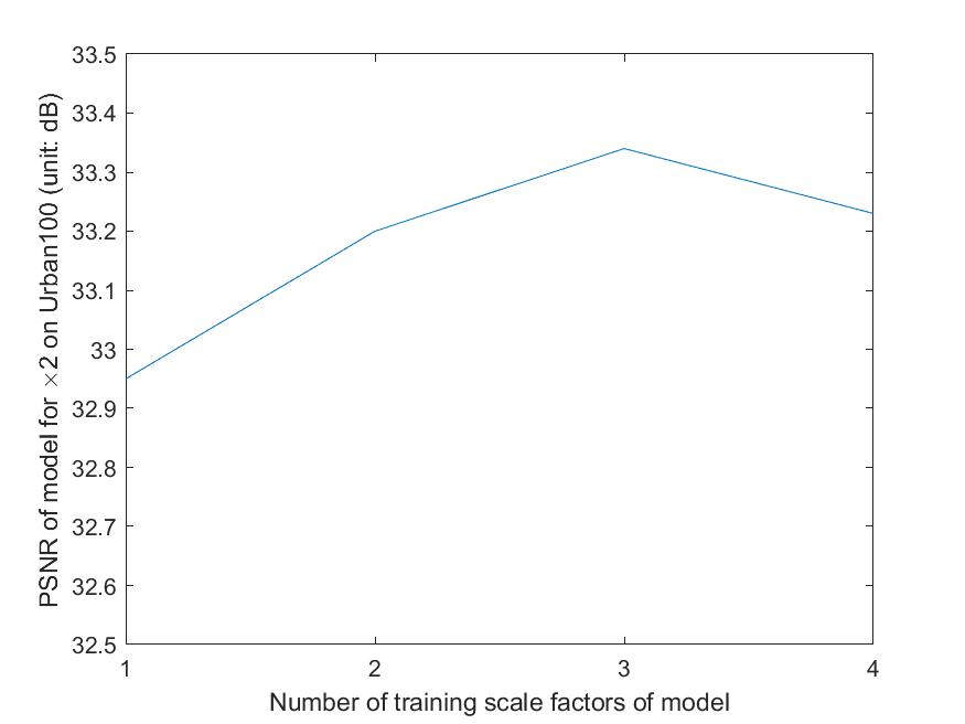
(a) Performance trend of models for $\times 2$

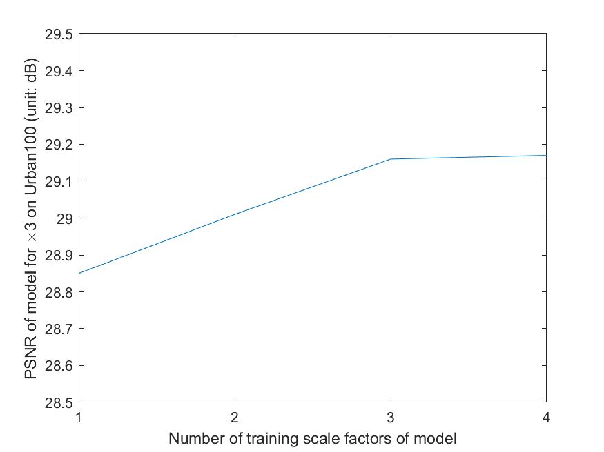
(b) Performance trend of models for $\times 3$

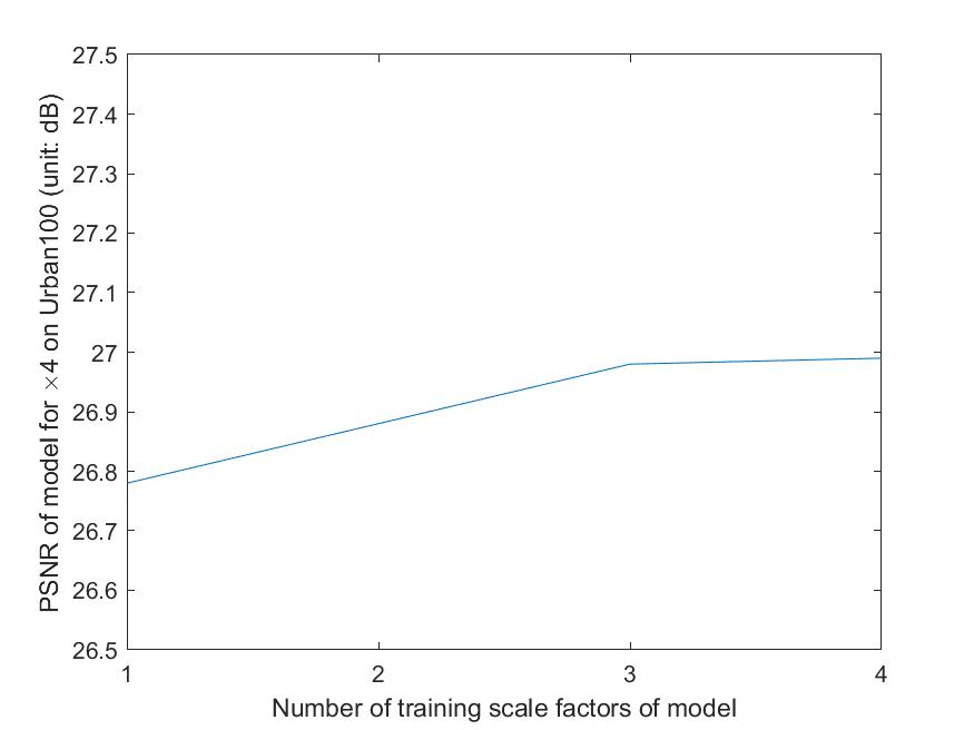
(c) Performance trend of models for $\times 4$

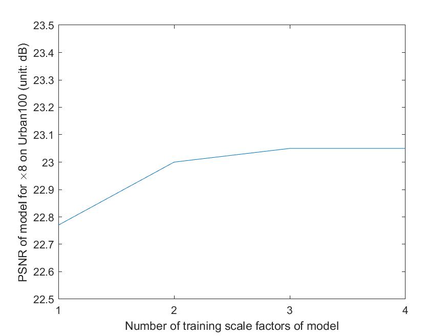
(d) Performance trend of models for $\times 8$

Figure 6. Illustration of effects to reconstruction performance of number of training scale factors. (a) Performance trend of models in group 2 for $\times 2$. (b) Performance trend of models in group 2 for $\times 3$. (c) Performance trend of models in group 3 for $\times 4$. (d) Performance trend of models in group 3 for $\times 8$.

4.3. Ablation Study

4.3.1. Effects of Multiple Scale Learning

In this subsection, we study the effects to performance of multiple scale training and the benefits to efficiency of multiple scale inference of our EMSRDPN model. We design three groups of experiments to study the effects to performance indices of number of training scale factors. First, we train four models each with only one RB tail for a different specific scale factor in set of scale factors $\times 2$, $\times 3$, $\times 4$ and $\times 8$, denoted as EMSRDPN-2, EMSRDPN-3, EMSRDPN-4, EMSRDPN-8. Second, we start with single scale model of scale factor $\times 2$, add one more scale factor each time according to the order of $\times 3$, $\times 4$, $\times 8$ to train model of two scale factors, three scale factors, four scale factors, denoted as EMSRDPN-2, EMSRDPN-23, EMSRDPN-234, EMSRDPN-2348. Third, we start with single scale model of scale factor $\times 8$, add one more scale factor each time according to the order of $\times 4$, $\times 3$, $\times 2$ to train model of two scale factors, three scale factors, four scale factors, denoted as EMSRDPN-8, EMSRDPN-48, EMSRDPN-348, EMSRDPN-2348. The same models in different groups are trained only once.

The performance comparison are shown in Table 1 and Figure 6. We have two observations. First, $\times 3$, $\times 4$, $\times 8$ all benefit from multiple scale training, the performance is increasing with the number of training scale factors. Second, $\times 2$ benefits from multiple scale training up to three training scale factors, including EMSRDPN-23, EMSRDPN-234 models, but the performance indices drop a little for the model of four training scale factors, i.e. EMSRDPN-2348. We argue that it is because patterns of LR images of large scale factor of $\times 8$ are much different from patterns of LR images of small scale factor of $\times 2$ which deteriorates the feature correlation of these two scale factors. According to these observations and analysis, we choose EMSRDPN-2348 as our final model abbreviated as EMSRDPN to compare to state-of-the-art SISR methods to achieve a good tradeoff between reconstruction performance and parameter and inference efficiency.

We also investigate the benefits to efficiency of multiple scale inference of our EMSRDPN model. As shown in Table 2, the multiple scale inference capability of our EMSRDPN model can amortize the parameters, memory consumption and computation flops between multiple scale factors. Our EMSRDPN model only add marginal parameters compared to a single scale model such as EMSRDPN-8, and only add marginal memory consumption and marginal computation flops to do inference of four scale factors compared to do inference of a single scale factor such as $\times 8$ using EMSRDPN-8. The overhead of multiple scale inference of our EMSRDPN model is only fourth of overhead of multiple scale inference using single scale models.

Table 3. Average PSNR/SSIM Metrics for Scale Factor $\times 4$ of EMSRDPN-Res-4, EMSRDPN-Dense-4 and EMSRDPN-4. Best is Highlighted, and Second Best is Underlined.

Method	Scale	Set5		Set14		B100		Urban100		Manga109
		PSNR	SSIM	PSNR	SSIM	PSNR	SSIM	PSNR	SSIM	PSNR	SSIM
EMSRDPN-Res-4	$\times 4$	32.52	0.9082	28.89	0.8050	27.73	0.7604	26.71	0.8179	31.17	0.9213
EMSRDPN-Dense-4	$\times 4$	32.52	0.9084	28.87	0.8049	27.74	0.7605	26.76	0.8186	31.28	0.9215
EMSRDPN-4	$\times 4$	32.50	0.9083	28.88	0.8048	27.74	0.7607	26.78	0.8188	31.28	0.9221

Table 4. Network Configuration and Inference Overhead for a $256\times 256$ Image of EMSRDPN-Res-4, EMSRDPN-Dense-4 and EMSRDPN-4. SSI: Single Scale Inference, MSI: Multiple Scale Inference.

Method	$G_{r}$	$G_{d}$	$G$	$G_{r}+G_{d}$	$D$	$C$	Params	Total Memory (MB)		Total Flops (T)
								SSI ($\times 4$)	MSI	SSI ($\times 4$)	MSI
EMSRDPN-Res-4	135	0	0	135	16	4	13,915,803	10677	✗	1.05	✗
EMSRDPN-Dense-4	0	122	122	122	16	4	13,748,671	12578	✗	1.01	✗
EMSRDPN-4	64	64	64	128	16	4	13,822,211	11660	✗	1.03	✗

4.3.2. Effects of Dual Path Connections

In this subsection, we study the effects of dual path connections proposed in our EMSRDPN model. Because residual connections and dense connections are special cases of the proposed dual path connections, we can simply set $G_{d}$ and $G$ to $0$ to form a model with a residual net structure or set $G_{r}$ to $0$ to form a model with a dense net structure. In this way, we can study the effects of dual path structure compared to pure residual net structure and dense net structure by limiting the models of three structures have similar number of parameters and similar number of network units thereof network depth. In this ablation study, we only train use models of different structure for $\times 4$ scale factor. Table 4 shows the network configuration of models of three structures, we use EMSRDPN-Res-4 to denote the model with only a residual net structure and EMSRDPN-Dense-4 to denote the model with only a dense net structure. Table 3 shows the performance comparisons for models of three structure. Table 4 also includes the total memory and total flops of models with different structures during inference to compare memory and computation overheads.

As shown in Table 3, EMSRDPN-4 has comparable even better performance compared to EMSRDPN-Res-4 and EMSRDPN-Dense-4. As shown in Table 4, the memory consumption of EMSRDPN-4 is less than EMSRDPN-Dense-4 and the computation flops of EMSRDPN-4 are less than EMSRDPN-Res-4. These observations demonstrate dual path structure can achieve a good trade-off between performance, memory consumption and computation overhead.

4.4. Comparisons with State-of-the-art Methods

Table 5. Average PSNR/SSIM Metrics for Scale Factors $\times 2$, $\times 3$, $\times 4$, $\times 8$ of Compared Methods. Best is Highlighted, and Second Best is Underlined.

Method	Scale	Set5		Set14		B100		Urban100		Manga109
		PSNR	SSIM	PSNR	SSIM	PSNR	SSIM	PSNR	SSIM	PSNR	SSIM
Bicubic	$\times 2$	33.66	0.9299	30.24	0.8688	29.56	0.8431	26.88	0.8403	30.80	0.9339
SRCNN (Dong et al., 2016b)	$\times 2$	36.66	0.9542	32.45	0.9067	31.36	0.8879	29.50	0.8946	35.60	0.9663
FSRCNN (Dong et al., 2016a)	$\times 2$	37.05	0.9560	32.66	0.9090	31.53	0.8920	29.88	0.9020	36.67	0.9710
VDSR (Kim et al., 2016a)	$\times 2$	37.53	0.9590	33.05	0.9130	31.90	0.8960	30.77	0.9140	37.22	0.9750
LapSRN (Lai et al., 2017)	$\times 2$	37.52	0.9591	33.08	0.9130	31.08	0.8950	30.41	0.9101	37.27	0.9740
MemNet (Tai et al., 2017b)	$\times 2$	37.78	0.9597	33.28	0.9142	32.08	0.8978	31.31	0.9195	37.72	0.9740
EDSR (Lim et al., 2017b)	$\times 2$	38.11	0.9602	33.92	0.9195	32.32	0.9013	32.93	0.9351	39.10	0.9773
SRMDNF (Zhang et al., 2018c)	$\times 2$	37.79	0.9601	33.32	0.9159	32.05	0.8985	31.33	0.9204	38.07	0.9761
D-DBPN (Haris et al., 2018)	$\times 2$	38.09	0.9600	33.85	0.9190	32.27	0.9000	32.55	0.9324	38.89	0.9775
RDN (Zhang et al., 2018b)	$\times 2$	38.24	0.9614	34.01	0.9212	32.34	0.9017	32.89	0.9353	39.18	0.9780
RCAN (Zhang et al., 2018a)	$\times 2$	38.27	0.9614	34.12	0.9216	32.41	0.9027	33.34	0.9384	39.44	0.9786
NLRN (Liu et al., 2018)	$\times 2$	38.00	0.9603	33.46	0.9159	32.19	0.8992	31.81	0.9249	-	-
MSRN (Li et al., 2018)	$\times 2$	38.08	0.9605	33.74	0.9170	32.23	0.9013	32.22	0.9326	38.82	0.9868
SAN (Dai et al., 2019)	$\times 2$	38.31	0.9620	34.07	0.9213	32.42	0.9028	33.10	0.9370	39.32	0.9792
HAN (Niu et al., 2020)	$\times 2$	38.27	0.9614	34.16	0.9217	32.41	0.9027	33.35	0.9385	39.46	0.9785
NLSN (Mei et al., 2021)	$\times 2$	38.34	0.9618	34.08	0.9231	32.43	0.9027	33.42	0.9394	39.59	0.9789
EMSRDPN-D	$\times 2$	38.23	0.9658	33.92	0.9289	32.33	0.9112	32.96	0.9408	39.11	0.9795
EMSRDPN	$\times 2$	38.22	0.9659	34.26	0.9309	32.40	0.9120	33.23	0.9436	39.46	0.9800
EMSRDPN+	$\times 2$	38.28	0.9660	34.31	0.9317	32.44	0.9124	33.45	0.9448	39.61	0.9804
Bicubic	$\times 3$	30.39	0.8682	27.55	0.7742	27.21	0.7385	24.46	0.7349	26.95	0.8556
SRCNN (Dong et al., 2016b)	$\times 3$	32.75	0.9090	29.30	0.8215	28.41	0.7863	26.24	0.7989	30.48	0.9117
FSRCNN (Dong et al., 2016a)	$\times 3$	33.18	0.9140	29.37	0.8240	28.53	0.7910	26.43	0.8080	31.10	0.9210
VDSR (Kim et al., 2016a)	$\times 3$	33.67	0.9210	29.78	0.8320	28.83	0.7990	27.14	0.8290	32.01	0.9340
LapSRN (Lai et al., 2017)	$\times 3$	33.82	0.9227	29.87	0.8320	28.82	0.7980	27.07	0.8280	32.21	0.9350
MemNet (Tai et al., 2017b)	$\times 3$	34.09	0.9248	30.00	0.8350	28.96	0.8001	27.56	0.8376	32.51	0.9369
EDSR (Lim et al., 2017b)	$\times 3$	34.65	0.9280	30.52	0.8462	29.25	0.8093	28.80	0.8653	34.17	0.9476
SRMDNF (Zhang et al., 2018c)	$\times 3$	34.12	0.9254	30.04	0.8382	28.97	0.8025	27.57	0.8398	33.00	0.9403
RDN (Zhang et al., 2018b)	$\times 3$	34.71	0.9296	30.57	0.8468	29.26	0.8093	28.80	0.8653	34.13	0.9484
RCAN (Zhang et al., 2018a)	$\times 3$	34.74	0.9299	30.65	0.8482	29.32	0.8111	29.09	0.8702	34.44	0.9499
NLRN (Liu et al., 2018)	$\times 3$	34.27	0.9266	30.16	0.8374	29.06	0.8026	27.93	0.8453	-	-
SAN (Dai et al., 2019)	$\times 3$	34.75	0.9300	30.59	0.8476	29.33	0.8112	28.93	0.8671	34.30	0.9494
HAN (Niu et al., 2020)	$\times 3$	34.75	0.9299	30.67	0.8483	29.32	0.8110	29.10	0.8705	34.48	0.9500
NLSN (Mei et al., 2021)	$\times 3$	34.85	0.9306	30.70	0.8485	29.34	0.8117	29.25	0.8726	34.57	0.9508
EMSRDPN-D	$\times 3$	34.74	0.9376	30.57	0.8619	29.26	0.8271	28.91	0.8775	34.24	0.9526
EMSRDPN	$\times 3$	34.80	0.9380	30.71	0.8637	29.31	0.8282	29.17	0.8818	34.61	0.9541
EMSRDPN+	$\times 3$	34.85	0.9384	30.78	0.8645	29.36	0.8289	29.31	0.8836	34.82	0.9550
Bicubic	$\times 4$	28.42	0.8104	26.00	0.7027	25.96	0.6675	23.14	0.6577	24.89	0.7866
SRCNN (Dong et al., 2016b)	$\times 4$	30.48	0.8628	27.50	0.7513	26.90	0.7101	24.52	0.7221	27.58	0.8555
FSRCNN (Dong et al., 2016a)	$\times 4$	30.72	0.8660	27.61	0.7550	26.98	0.7150	24.62	0.7280	27.90	0.8610
VDSR (Kim et al., 2016a)	$\times 4$	31.35	0.8830	28.02	0.7680	27.29	0.0726	25.18	0.7540	28.83	0.8870
LapSRN (Lai et al., 2017)	$\times 4$	31.54	0.8850	28.19	0.7720	27.32	0.7270	25.21	0.7560	29.09	0.8900
MemNet (Tai et al., 2017b)	$\times 4$	31.74	0.8893	28.26	0.7723	27.40	0.7281	25.50	0.7630	29.42	0.8942
EDSR (Lim et al., 2017b)	$\times 4$	32.46	0.8968	28.80	0.7876	27.71	0.7420	26.64	0.8033	31.02	0.9148
SRMDNF (Zhang et al., 2018c)	$\times 4$	31.96	0.8925	28.35	0.7787	27.49	0.7337	25.68	0.7731	30.09	0.9024
D-DBPN (Haris et al., 2018)	$\times 4$	32.47	0.8980	28.82	0.7860	27.72	0.7400	26.38	0.7946	30.91	0.9137
RDN (Zhang et al., 2018b)	$\times 4$	32.47	0.8990	28.81	0.7871	27.72	0.7419	26.61	0.8028	31.00	0.9151
RCAN (Zhang et al., 2018a)	$\times 4$	32.63	0.9002	28.87	0.7889	27.77	0.7436	26.82	0.8087	31.22	0.9173
NLRN (Liu et al., 2018)	$\times 4$	31.92	0.8916	28.36	0.7745	27.48	0.7306	25.79	0.7729	-	-
MSRN (Li et al., 2018)	$\times 4$	32.07	0.8903	28.60	0.7751	27.52	0.7273	26.04	0.7896	30.17	0.9034
SAN (Dai et al., 2019)	$\times 4$	32.64	0.9003	28.92	0.7888	27.78	0.7436	26.79	0.8068	31.18	0.9169
HAN (Niu et al., 2020)	$\times 4$	32.64	0.9002	28.90	0.7890	27.80	0.7442	26.85	0.8094	31.42	0.9177
NLSN (Mei et al., 2021)	$\times 4$	32.59	0.9000	28.87	0.7891	27.78	0.7444	26.96	0.8109	31.27	0.9184
EMSRDPN-D	$\times 4$	32.50	0.9080	28.85	0.8052	27.74	0.7609	26.79	0.8198	31.20	0.9216
EMSRDPN	$\times 4$	32.62	0.9093	28.93	0.8069	27.79	0.7627	26.99	0.8253	31.50	0.9233
EMSRDPN+	$\times 4$	32.70	0.9101	29.02	0.8081	27.84	0.7637	27.14	0.8279	31.74	0.9252
Bicubic	$\times 8$	24.40	0.6580	23.10	0.5660	23.67	0.5480	20.74	0.5160	21.47	0.6500
SRCNN (Dong et al., 2016b)	$\times 8$	25.33	0.6900	23.76	0.5910	24.13	0.5660	21.29	0.5440	22.46	0.6950
FSRCNN (Dong et al., 2016a)	$\times 8$	20.13	0.5520	19.75	0.4820	24.21	0.5680	21.32	0.5380	22.39	0.6730
SCN (Wang et al., 2015)	$\times 8$	25.59	0.7071	24.02	0.6028	24.30	0.5698	21.52	0.5571	22.68	0.6963
VDSR (Kim et al., 2016a)	$\times 8$	25.93	0.7240	24.26	0.6140	24.49	0.5830	21.70	0.5710	23.16	0.7250
LapSRN (Lai et al., 2017)	$\times 8$	26.15	0.7380	24.35	0.6200	24.54	0.5860	21.81	0.5810	23.39	0.7350
MemNet (Tai et al., 2017b)	$\times 8$	26.16	0.7414	24.38	0.6199	24.58	0.5842	21.89	0.5825	23.56	0.7387
MSLapSRN (Lai et al., 2018)	$\times 8$	26.34	0.7530	24.57	0.6290	24.65	0.5920	22.06	0.5980	23.90	0.7590
EDSR (Lim et al., 2017b)	$\times 8$	26.96	0.7762	24.91	0.6420	24.81	0.5985	22.51	0.6221	24.69	0.7841
D-DBPN (Haris et al., 2018)	$\times 8$	27.21	0.7840	25.13	0.6480	24.88	0.6010	22.73	0.6312	25.14	0.7987
RCAN (Zhang et al., 2018a)	$\times 8$	27.31	0.7878	25.23	0.6511	24.98	0.6058	23.00	0.6452	25.24	0.8029
MSRN (Li et al., 2018)	$\times 8$	26.59	0.7254	24.88	0.5961	24.70	0.5410	22.37	0.5977	24.28	0.7517
SAN (Dai et al., 2019)	$\times 8$	27.22	0.7829	25.14	0.6476	24.88	0.6011	22.70	0.6314	24.85	0.7906
HAN (Niu et al., 2020)	$\times 8$	27.33	0.7884	25.24	0.6510	24.98	0.6059	22.98	0.6437	25.20	0.8011
EMSRDPN-D	$\times 8$	27.28	0.7836	25.18	0.6514	24.93	0.6049	22.88	0.6456	25.09	0.7972
EMSRDPN	$\times 8$	27.34	0.7858	25.29	0.6547	24.96	0.6066	23.05	0.6525	25.30	0.8025
EMSRDPN+	$\times 8$	27.41	0.7873	25.37	0.6564	25.01	0.6078	23.18	0.6566	25.50	0.8067

B100 ($\times 4$)
78004

HR
PSNR/SSIM

Bicubic
24.47/0.6480

LapSRN
26.19/0.7422

MDSR
27.00/0.7681

D-DBPN
26.92/0.7642

RDN
27.14/0.7755

RCAN
27.40/0.7795

MSRN
26.92/0.7621

SAN
27.18/0.7748

HAN
27.51/0.7801

NLSN
27.29/0.7760

EMSRDPN
27.51/0.7833

Manga109 ($\times 4$)
OL_Lunch

HR
PSNR/SSIM

Bicubic
20.79/0.8335

LapSRN
27.04/0.9449

MDSR
28.09/0.9524

D-DBPN
27.45/0.9511

RDN
28.05/0.9527

RCAN
27.96/0.9529

MSRN
27.51/0.9481

SAN
28.24/0.9537

HAN
27.42/0.9473

NLSN
28.50/0.9554

EMSRDPN
28.43/0.9560

Figure 7. Visual comparison for $\times 4$ on B100 and Manga109 datasets.

Urban100 ($\times 8$)
img028

HR
PSNR/SSIM

Bicubic
25.44/0.7179

LapSRN
27.02/0.7787

D-DBPN
27.14/0.7804

RCAN
27.74/0.7961

MSRN
27.16/0.7782

HAN
27.66/0.7948

EMSRDPN
28.07/0.8032

Urban100 ($\times 8$)
img092

HR
PSNR/SSIM

Bicubic
15.43/0.3268

LapSRN
15.80/0.3983

D-DBPN
16.18/0.4417

RCAN
16.35/0.4374

MSRN
15.83/0.4002

HAN
16.38/0.4420

EMSRDPN
16.74/0.4771

Manga109 ($\times 8$)
MisutenaideDaisy

HR
PSNR/SSIM

Bicubic
22.61/0.7747

LapSRN
26.14/0.9018

D-DBPN
27.33/0.9242

RCAN
27.58/0.9254

MSRN
26.62/0.9093

HAN
27.49/0.9245

EMSRDPN
27.65/0.9269

Figure 8. Visual comparison for $\times 8$ on Urban100 and Manga109 datasets.

In this subsection, we compare our method with SRCNN (Dong et al., 2016b), FSRCNN (Dong et al., 2016a), VDSR (Kim et al., 2016a), LapSRN (Lai et al., 2017), MemNet (Tai et al., 2017b), EDSR (Lim et al., 2017b), SRMDNF (Zhang et al., 2018c), D-DBPN (Haris et al., 2018), RDN (Zhang et al., 2018b), RCAN (Zhang et al., 2018a), MSRN (Li et al., 2018), NLRN (Liu et al., 2018), SAN (Dai et al., 2019), HAN (Niu et al., 2020) and NLSN (Mei et al., 2021) to validate the effectiveness of EMSRDPN. Following the literature, self-ensemble strategy (Lim et al., 2017b) is also adopted to improve EMSRDPN and self-ensembled EMSRDPN is denoted as EMSRDPN+. Table 5 shows the peak signal-to-noise ratio (PSNR) and the structural similarity index measure (SSIM) metrics on five benchmark datasets. Our method achieves comparable even better performance over state-of-the-art methods on almost all combinations of benchmark datasets and scale factors.

Figure 7, 8 show visual comparisons. As shown in image $78004$ from B100, images $img028$ and $img092$ from Urban100, our method reconstructs more textures, less blurring and ring effects of images than other state-of-the-art methods. As shown in images $OLLunch$ and $MisutenaideDaisy$ from Manga109, our method reconstructs clearer edges and less artifacts of images than other state-of-the-art methods. Visual comparisons show our method reconstructs more high frequency details such as edges and textures of images and has less artifacts.

4.5. Model Complexity and Inference Time

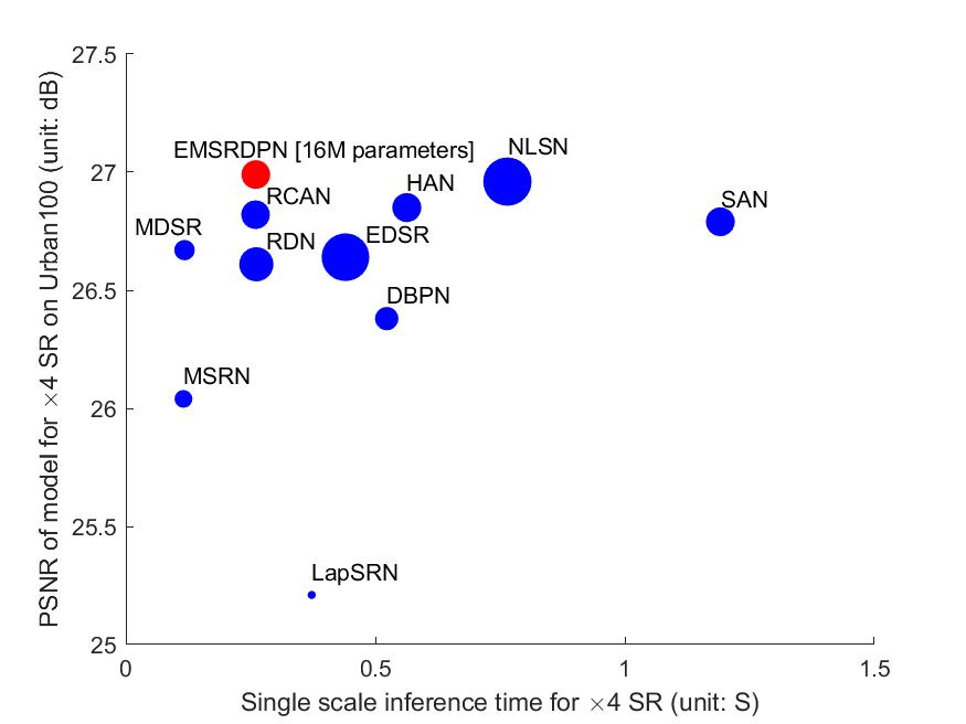
(a) Comparison for single scale inference

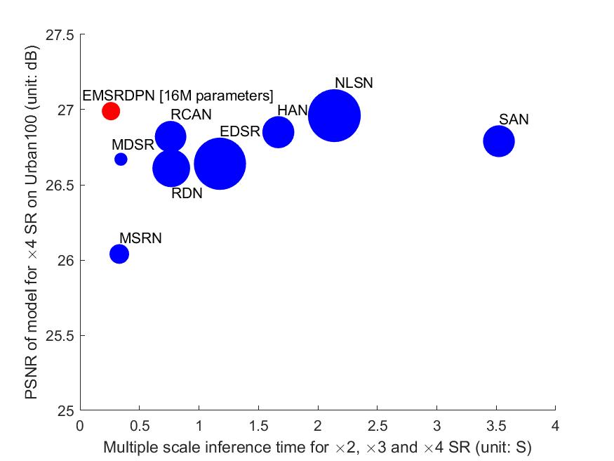
(b) Comparison for multiple scale inference

Figure 9. Comparison of the performance, number of parameters and inference time of models, the inference time is tested using a $256\times 256$ image on a NVIDIA TITAN Xp GPU. (a) Comparison for single scale inference of $\times 4$, the size of solid circle is proportional to number of parameters of model for $\times 4$. (b) Comparison for multiple scale inference of $\times 2$, $\times 3$, and $\times 4$, the size of solid circle is proportional to number of parameters of models for $\times 2$, $\times 3$ and $\times 4$.

In this subsection, we compare number of parameters and inference time of our EMSRDPN model with state-of-the-art methods. For single scale inference such as $\times 4$ as shown in Figure 9(a), our method has more parameters or inference time than LapSRN (Lai et al., 2017), MDSR (Lim et al., 2017b), MSRN (Li et al., 2018) and DBPN (Haris et al., 2018) but it has much better reconstruction performance, meanwhile, our method has comparable even much less parameters and inference time than other state-of-the-art methods except that it has better reconstruction performance than these state-of-the-art methods. The efficiency of our method is much obvious especially for multiple scale inference such as $\times 2$, $\times 3$, and $\times 4$ as shown in Figure 9(b), our method has comparable parameters and inference time to MDSR (Lim et al., 2017b) and MSRN (Li et al., 2018) and much less parameters and inference time than other state-of-the-art methods, but it has much better reconstruction performance than MDSR (Lim et al., 2017b) and MSRN (Li et al., 2018) and better reconstruction performance than other state-of-the-art methods. It is worth noting that the additional multiple scale inference time of $\times 2$, $\times 3$, and $\times 4$ is only marginal compared to the single scale inference time of $\times 4$, because the most computation can be shared between different scale factors during inference, which is consistent with results in Table 2 and Section 4.3.1. The statistics of number of parameters and inference time in this subsection and reconstruction performance in previous subsection show that our method can achieve a good trade-off between number of parameters, inference time and reconstruction performance.

5. Conclusion and Future Work

In this work, we propose an efficient single image super-resolution network using dual path connections with multiple scale learning named as EMSRDPN to boost reconstruction performance, save parameters and improve computation efficiency for SISR. First, we introduce efficient dual path connections into a very deep convolutional neural network, which have the benefits of both residual connections to reuse common features and dense connections to explore new features to learn a good representation for SISR. Second, based on the improved network architecture to do SISR in LR space to save computation and memory cost, we propose a multiple scale training and inference architecture of network by sharing most of network parameters between different scale factors to make use of training data of multiple scale factors for each other to utilize feature correlation during training and amortize most parameters and computation between multiple scale factors during inference, which has benefits of both achieving better performance and improving parameter efficiency and inference time of network. Experiments show that our new model achieves better performance and improved visual effects can be seen in the results compared to state-of-the-art methods. Meanwhile, our method has comparable or even better parameter efficiency and inference time compared to state-of-the-art methods. We believe the proposed multiple scale training and inference strategy is generally applicable to various network designs to boost performance and efficiency of SISR and dual path connections could also be useful to other multimedia tasks than SISR.

References

- (1)
- Agustsson and Timofte (2017) Eirikur Agustsson and Radu Timofte. 2017. NTIRE 2017 Challenge on Single Image Super-Resolution: Dataset and Study. 2017 IEEE Conference on Computer Vision and Pattern Recognition Workshops (CVPRW) (2017), 1122–1131.
- Allebach and Wong (1996) Jan P. Allebach and Ping Wah Wong. 1996. Edge-directed interpolation. In Proceedings 1996 International Conference on Image Processing, Lausanne, Switzerland, September 16-19, 1996. IEEE Computer Society, 707–710. https://doi.org/10.1109/ICIP.1996.560768
- Anwar and Barnes (2022) Saeed Anwar and Nick Barnes. 2022. Densely Residual Laplacian Super-Resolution. IEEE Transactions on Pattern Analysis and Machine Intelligence 44 (2022), 1192–1204.
- Bevilacqua et al. (2012) Marco Bevilacqua, Aline Roumy, Christine Guillemot, and Marie line Alberi Morel. 2012. Low-Complexity Single-Image Super-Resolution based on Nonnegative Neighbor Embedding. In Proceedings of the British Machine Vision Conference. BMVA Press, 135.1–135.10. https://doi.org/10.5244/C.26.135
- Chang et al. (2004) Hong Chang, Dit-Yan Yeung, and Yimin Xiong. 2004. Super-resolution through neighbor embedding. In Proceedings of the 2004 IEEE Computer Society Conference on Computer Vision and Pattern Recognition, 2004. CVPR 2004., Vol. 1. IEEE, I–I.
- Chen et al. (2017) Yunpeng Chen, Jianan Li, Huaxin Xiao, Xiaojie Jin, Shuicheng Yan, and Jiashi Feng. 2017. Dual path networks. In Advances in Neural Information Processing Systems. 4467–4475.
- Dai et al. (2019) Tao Dai, Jianrui Cai, Yongbing Zhang, Shu-Tao Xia, and Lei Zhang. 2019. Second-Order Attention Network for Single Image Super-Resolution. In IEEE Conference on Computer Vision and Pattern Recognition, CVPR 2019, Long Beach, CA, USA, June 16-20, 2019. Computer Vision Foundation / IEEE, 11065–11074. https://doi.org/10.1109/CVPR.2019.01132
- Deng et al. (2009) Jia Deng, Wei Dong, Richard Socher, Li-Jia Li, Kai Li, and Li Fei-Fei. 2009. ImageNet: A large-scale hierarchical image database. 2009 IEEE Conference on Computer Vision and Pattern Recognition (2009), 248–255.
- Dong et al. (2016b) Chao Dong, Chen Change Loy, Kaiming He, and Xiaoou Tang. 2016b. Image super-resolution using deep convolutional networks. IEEE transactions on pattern analysis and machine intelligence 38, 2 (2016), 295–307.
- Dong et al. (2016a) Chao Dong, Chen Change Loy, and Xiaoou Tang. 2016a. Accelerating the super-resolution convolutional neural network. In European conference on computer vision. Springer, 391–407.
- Dong et al. (2011) Weisheng Dong, Lei Zhang, Guangming Shi, and Xiaolin Wu. 2011. Image Deblurring and Super-Resolution by Adaptive Sparse Domain Selection and Adaptive Regularization. IEEE Trans. Image Process. 20, 7 (2011), 1838–1857. https://doi.org/10.1109/TIP.2011.2108306
- Freeman et al. (2002) William T Freeman, Thouis R Jones, and Egon C Pasztor. 2002. Example-based super-resolution. IEEE Computer graphics and Applications 22, 2 (2002), 56–65.
- Freeman and Pasztor (1999) William T. Freeman and Egon C. Pasztor. 1999. Learning Low-Level Vision. In Proceedings of the International Conference on Computer Vision, Kerkyra, Corfu, Greece, September 20-25, 1999. IEEE Computer Society, 1182–1189. https://doi.org/10.1109/ICCV.1999.790414
- Fujimoto et al. (2016) Azuma Fujimoto, Toru Ogawa, Kazuyoshi Yamamoto, Yusuke Matsui, Toshihiko Yamasaki, and Kiyoharu Aizawa. 2016. Manga109 dataset and creation of metadata. In Proceedings of the 1st International Workshop on coMics ANalysis, Processing and Understanding, MANPU@ICPR 2016, Cancun, Mexico, December 4, 2016, Jean-Marc Ogier, Kiyoharu Aizawa, Koichi Kise, Jean-Christophe Burie, Toshihiko Yamasaki, and Motoi Iwata (Eds.). ACM, 2:1–2:5. https://doi.org/10.1145/3011549.3011551
- Glasner et al. (2009) Daniel Glasner, Shai Bagon, and Michal Irani. 2009. Super-resolution from a single image. In 2009 IEEE 12th international conference on computer vision. IEEE, 349–356.
- Haris et al. (2018) Muhammad Haris, Gregory Shakhnarovich, and Norimichi Ukita. 2018. Deep back-projection networks for super-resolution. In Proceedings of the IEEE conference on computer vision and pattern recognition. 1664–1673.
- He et al. (2016) Kaiming He, Xiangyu Zhang, Shaoqing Ren, and Jian Sun. 2016. Identity mappings in deep residual networks. In European conference on computer vision. Springer, 630–645.
- Huang et al. (2015) Jia-Bin Huang, Abhishek Singh, and Narendra Ahuja. 2015. Single image super-resolution from transformed self-exemplars. In Proceedings of the IEEE Conference on Computer Vision and Pattern Recognition. 5197–5206.
- Hui et al. (2018) Zheng Hui, Xiumei Wang, and Xinbo Gao. 2018. Fast and accurate single image super-resolution via information distillation network. In Proceedings of the IEEE Conference on Computer Vision and Pattern Recognition. 723–731.
- Ioffe and Szegedy (2015) Sergey Ioffe and Christian Szegedy. 2015. Batch Normalization: Accelerating Deep Network Training by Reducing Internal Covariate Shift. In Proceedings of the 32nd International Conference on Machine Learning (Proceedings of Machine Learning Research, Vol. 37), Francis Bach and David Blei (Eds.). PMLR, Lille, France, 448–456. http://proceedings.mlr.press/v37/ioffe15.html
- Irani and Peleg (1991) Michal Irani and Shmuel Peleg. 1991. Improving resolution by image registration. CVGIP: Graphical Model and Image Processing 53 (1991), 231–239.
- Johnson et al. (2016) Justin Johnson, Alexandre Alahi, and Li Fei-Fei. 2016. Perceptual losses for real-time style transfer and super-resolution. In European conference on computer vision. Springer, 694–711.
- Kim et al. (2016a) Jiwon Kim, Jung Kwon Lee, and Kyoung Mu Lee. 2016a. Accurate image super-resolution using very deep convolutional networks. In Proceedings of the IEEE conference on computer vision and pattern recognition. 1646–1654.
- Kim et al. (2016b) Jiwon Kim, Jung Kwon Lee, and Kyoung Mu Lee. 2016b. Deeply-Recursive Convolutional Network for Image Super-Resolution. In 2016 IEEE Conference on Computer Vision and Pattern Recognition, CVPR 2016, Las Vegas, NV, USA, June 27-30, 2016. IEEE Computer Society, 1637–1645. https://doi.org/10.1109/CVPR.2016.181
- Kingma and Ba (2015) Diederik P. Kingma and Jimmy Ba. 2015. Adam: A Method for Stochastic Optimization. In 3rd International Conference on Learning Representations, ICLR 2015, San Diego, CA, USA, May 7-9, 2015, Conference Track Proceedings, Yoshua Bengio and Yann LeCun (Eds.). http://arxiv.org/abs/1412.6980
- Lai et al. (2017) Wei-Sheng Lai, Jia-Bin Huang, Narendra Ahuja, and Ming-Hsuan Yang. 2017. Deep laplacian pyramid networks for fast and accurate super-resolution. In Proceedings of the IEEE conference on computer vision and pattern recognition. 624–632.
- Lai et al. (2018) Wei-Sheng Lai, Jia-Bin Huang, Narendra Ahuja, and Ming-Hsuan Yang. 2018. Fast and accurate image super-resolution with deep laplacian pyramid networks. IEEE transactions on pattern analysis and machine intelligence 41, 11 (2018), 2599–2613.
- Ledig et al. (2017) Christian Ledig, Lucas Theis, Ferenc Huszár, Jose Caballero, Andrew Cunningham, Alejandro Acosta, Andrew Aitken, Alykhan Tejani, Johannes Totz, Zehan Wang, et al. 2017. Photo-realistic single image super-resolution using a generative adversarial network. In Proceedings of the IEEE conference on computer vision and pattern recognition. 4681–4690.
- Li et al. (2018) Juncheng Li, Faming Fang, Kangfu Mei, and Guixu Zhang. 2018. Multi-scale residual network for image super-resolution. In Proceedings of the European Conference on Computer Vision (ECCV). 517–532.
- Li and Orchard (2001) Xin Li and Michael T. Orchard. 2001. New edge-directed interpolation. IEEE Trans. Image Process. 10, 10 (2001), 1521–1527. https://doi.org/10.1109/83.951537
- Li et al. (2021) Yanchun Li, Jianglian Cao, Zhetao Li, Sangyoon Oh, and Nobuyoshi Komuro. 2021. Lightweight Single Image Super-resolution with Dense Connection Distillation Network. ACM Transactions on Multimedia Computing, Communications, and Applications (TOMM) 17, 1s (2021), 1–17.
- Liebel and Körner (2016) Lukas Liebel and Marco Körner. 2016. Single-image super resolution for multispectral remote sensing data using convolutional neural networks. ISPRS-International Archives of the Photogrammetry, Remote Sensing and Spatial Information Sciences 41 (2016), 883–890.
- Lim et al. (2017a) Bee Lim, Sanghyun Son, Heewon Kim, Seungjun Nah, and Kyoung Mu Lee. 2017a. Enhanced Deep Residual Networks for Single Image Super-Resolution. In The IEEE Conference on Computer Vision and Pattern Recognition (CVPR) Workshops.
- Lim et al. (2017b) Bee Lim, Sanghyun Son, Heewon Kim, Seungjun Nah, and Kyoung Mu Lee. 2017b. Enhanced deep residual networks for single image super-resolution. In Proceedings of the IEEE Conference on Computer Vision and Pattern Recognition Workshops. 136–144.
- Liu et al. (2018) Ding Liu, Bihan Wen, Yuchen Fan, Chen Change Loy, and Thomas S. Huang. 2018. Non-Local Recurrent Network for Image Restoration. In Advances in Neural Information Processing Systems 31: Annual Conference on Neural Information Processing Systems 2018, NeurIPS 2018, December 3-8, 2018, Montréal, Canada, Samy Bengio, Hanna M. Wallach, Hugo Larochelle, Kristen Grauman, Nicolò Cesa-Bianchi, and Roman Garnett (Eds.). 1680–1689. https://proceedings.neurips.cc/paper/2018/hash/fc49306d97602c8ed1be1dfbf0835ead-Abstract.html
- Mao et al. (2016) Xiaojiao Mao, Chunhua Shen, and Yu-Bin Yang. 2016. Image restoration using very deep convolutional encoder-decoder networks with symmetric skip connections. In Advances in neural information processing systems. 2802–2810.
- Martin et al. (2001) David R. Martin, Charless C. Fowlkes, Doron Tal, and Jitendra Malik. 2001. A Database of Human Segmented Natural Images and its Application to Evaluating Segmentation Algorithms and Measuring Ecological Statistics. In Proceedings of the Eighth International Conference On Computer Vision (ICCV-01), Vancouver, British Columbia, Canada, July 7-14, 2001 - Volume 2. IEEE Computer Society, 416–425. https://doi.org/10.1109/ICCV.2001.937655
- Mei et al. (2021) Yiqun Mei, Yuchen Fan, and Yuqian Zhou. 2021. Image Super-Resolution With Non-Local Sparse Attention. In Proceedings of the IEEE/CVF Conference on Computer Vision and Pattern Recognition. 3517–3526.
- Niu et al. (2020) Ben Niu, Weilei Wen, Wenqi Ren, Xiangde Zhang, Lianping Yang, Shuzhen Wang, Kaihao Zhang, Xiaochun Cao, and Haifeng Shen. 2020. Single image super-resolution via a holistic attention network. In European Conference on Computer Vision. Springer, 191–207.
- Qiu et al. (2019) Yajun Qiu, Ruxin Wang, Dapeng Tao, and Jun Cheng. 2019. Embedded Block Residual Network: A Recursive Restoration Model for Single-Image Super-Resolution. In 2019 IEEE/CVF International Conference on Computer Vision, ICCV 2019, Seoul, Korea (South), October 27 - November 2, 2019. IEEE, 4179–4188. https://doi.org/10.1109/ICCV.2019.00428
- Sajjadi et al. (2017) Msm Sajjadi, B. Scholkopf, and M. Hirsch. 2017. EnhanceNet: Single Image Super-Resolution Through Automated Texture Synthesis. In IEEE International Conference on Computer Vision.
- Shi et al. (2016) Wenzhe Shi, Jose Caballero, Ferenc Huszár, Johannes Totz, Andrew P Aitken, Rob Bishop, Daniel Rueckert, and Zehan Wang. 2016. Real-time single image and video super-resolution using an efficient sub-pixel convolutional neural network. In Proceedings of the IEEE conference on computer vision and pattern recognition. 1874–1883.
- Shi et al. (2013) Wenzhe Shi, Jose Caballero, Christian Ledig, Xiahai Zhuang, Wenjia Bai, Kanwal K. Bhatia, Antonio M. Simoes Monteiro de Marvao, Tim Dawes, Declan P. O’Regan, and Daniel Rueckert. 2013. Cardiac Image Super-Resolution with Global Correspondence Using Multi-Atlas PatchMatch. In Medical Image Computing and Computer-Assisted Intervention - MICCAI 2013 - 16th International Conference, Nagoya, Japan, September 22-26, 2013, Proceedings, Part III (Lecture Notes in Computer Science, Vol. 8151), Kensaku Mori, Ichiro Sakuma, Yoshinobu Sato, Christian Barillot, and Nassir Navab (Eds.). Springer, 9–16. https://doi.org/10.1007/978-3-642-40760-4_2
- Sun et al. (2008) Jian Sun, Zongben Xu, and Heung-Yeung Shum. 2008. Image super-resolution using gradient profile prior. In 2008 IEEE Conference on Computer Vision and Pattern Recognition. IEEE, 1–8.
- Tai et al. (2017a) Ying Tai, Jian Yang, and Xiaoming Liu. 2017a. Image super-resolution via deep recursive residual network. In Proceedings of the IEEE Conference on Computer vision and Pattern Recognition. 3147–3155.
- Tai et al. (2017b) Ying Tai, Jian Yang, Xiaoming Liu, and Chunyan Xu. 2017b. Memnet: A persistent memory network for image restoration. In Proceedings of the IEEE International Conference on Computer Vision. 4539–4547.
- Tai et al. (2010) Yu-Wing Tai, Shuaicheng Liu, Michael S Brown, and Stephen Lin. 2010. Super resolution using edge prior and single image detail synthesis. In 2010 IEEE computer society conference on computer vision and pattern recognition. IEEE, 2400–2407.
- Timofte et al. (2014) Radu Timofte, Vincent De Smet, and Luc Van Gool. 2014. A+: Adjusted anchored neighborhood regression for fast super-resolution. In Asian conference on computer vision. Springer, 111–126.
- Tong et al. (2017) Tong Tong, Gen Li, Xiejie Liu, and Qinquan Gao. 2017. Image super-resolution using dense skip connections. In Proceedings of the IEEE International Conference on Computer Vision. 4799–4807.
- Wang et al. (2015) Zhaowen Wang, Ding Liu, Jianchao Yang, Wei Han, and Thomas Huang. 2015. Deep networks for image super-resolution with sparse prior. In Proceedings of the IEEE international conference on computer vision. 370–378.
- Xu et al. (2016) Lie Xu, Chiu-sing Choy, and Yi-Wen Li. 2016. Deep sparse rectifier neural networks for speech denoising. In IEEE International Workshop on Acoustic Signal Enhancement, IWAENC 2016, Xi’an, China, September 13-16, 2016. IEEE, 1–5. https://doi.org/10.1109/IWAENC.2016.7602891
- Yang (2019) Bin-Cheng Yang. 2019. Super Resolution Using Dual Path Connections. In Proceedings of the 27th ACM International Conference on Multimedia (Nice, France) (MM ’19). Association for Computing Machinery, New York, NY, USA, 1552–1560. https://doi.org/10.1145/3343031.3350878
- Yang and Yang (2013) Chih-Yuan Yang and Ming-Hsuan Yang. 2013. Fast direct super-resolution by simple functions. In Proceedings of the IEEE international conference on computer vision. 561–568.
- Yang et al. (2010) Jianchao Yang, John Wright, Thomas S Huang, and Yi Ma. 2010. Image super-resolution via sparse representation. IEEE transactions on image processing 19, 11 (2010), 2861–2873.
- Zeyde et al. (2010) Roman Zeyde, Michael Elad, and Matan Protter. 2010. On single image scale-up using sparse-representations. In International conference on curves and surfaces. Springer, 711–730.
- Zhang et al. (2020a) Dongyang Zhang, Jie Shao, and Heng Tao Shen. 2020a. Kernel attention network for single image super-resolution. ACM Transactions on Multimedia Computing, Communications, and Applications (TOMM) 16, 3 (2020), 1–15.
- Zhang et al. (2012) Kaibing Zhang, Xinbo Gao, Dacheng Tao, and Xuelong Li. 2012. Single Image Super-Resolution With Non-Local Means and Steering Kernel Regression. IEEE Transactions on Image Processing 21 (2012), 4544–4556.
- Zhang et al. (2018c) Kai Zhang, Wangmeng Zuo, and Lei Zhang. 2018c. Learning a Single Convolutional Super-Resolution Network for Multiple Degradations. In 2018 IEEE Conference on Computer Vision and Pattern Recognition, CVPR 2018, Salt Lake City, UT, USA, June 18-22, 2018. Computer Vision Foundation / IEEE Computer Society, 3262–3271. https://doi.org/10.1109/CVPR.2018.00344
- Zhang and Wu (2006) Lei Zhang and Xiaolin Wu. 2006. An edge-guided image interpolation algorithm via directional filtering and data fusion. IEEE Transactions on Image Processing 15 (2006), 2226–2238.
- Zhang et al. (2018a) Yulun Zhang, Kunpeng Li, Kai Li, Lichen Wang, Bineng Zhong, and Yun Fu. 2018a. Image super-resolution using very deep residual channel attention networks. In Proceedings of the European Conference on Computer Vision (ECCV). 286–301.
- Zhang et al. (2019) Yulun Zhang, Kunpeng Li, Kai Li, Bineng Zhong, and Yun Fu. 2019. Residual non-local attention networks for image restoration. arXiv preprint arXiv:1903.10082 (2019).
- Zhang et al. (2018b) Yulun Zhang, Yapeng Tian, Yu Kong, Bineng Zhong, and Yun Fu. 2018b. Residual dense network for image super-resolution. In Proceedings of the IEEE Conference on Computer Vision and Pattern Recognition. 2472–2481.
- Zhang et al. (2020b) Yulun Zhang, Yapeng Tian, Yu Kong, Bineng Zhong, and Yun Fu. 2020b. Residual dense network for image restoration. IEEE Transactions on Pattern Analysis and Machine Intelligence 43, 7 (2020), 2480–2495.
- Zou and Yuen (2010) Wilman W. W. Zou and Pong Chi Yuen. 2010. Very low resolution face recognition problem. 2010 Fourth IEEE International Conference on Biometrics: Theory, Applications and Systems (BTAS) (2010), 1–6.