The Sackin Index of Simplex Networks

Abstract

A phylogenetic network is a simplex (or 1-component tree-child) network if the child of every reticulation node is a network leaf. Simplex networks are a superclass of phylogenetic trees and a subclass of tree-child networks. Generalizing the Sackin index to phylogenetic networks, we prove that the expected Sacking index of a random simplex network is asymptotically $\Omega(n^{7/4})$ in the uniform model.

[inst1]organization=Department of Mathematics and Centre of Data Science and Machine Learning, National University of Singapore, addressline=10 Lower Kent Ridge Road, country=Singapore 119076

1 Introduction

Phylogenetic networks have been frequently used for modeling evolutionary history of genomes and genetic flow in population genetics. Since network models are much more complex than phylgoenetic trees, different classes of phylgoenetic networks have been introduced to investigate different issues of reconstruction of phylogenetic networks [1, 2, 3, 4]. For these special classes of phylogenetic networks, algorithmic problems for determining the relationship between phylogenetic trees and networks and for reconstruction of phylogenetic networks from DNA sequences, gene trees and other data have been extensively studied [5, 6, 7].

The combinatorial and stochastic properties of different classes of phylogenetic networks has received increasing attention in the study of phylogenetic networks recently. Counting tree-child networks was first studied in [8]. A tight asymptotic value of the number of tree-child networks is given in [9]. Although algorithms are presented for enumerating tree-child networks [10, 11], closed formulas and even simple recurrence formulas for counting tree-child networks are unknown [12, 13]. Counting ranked tree-child networks is studied in [14]. In addition, asymptotic and exact counts of galled trees and galled networks are given in [15] and [16, 17], respectively.

The expected height of random binary trees has been known for decades [18]. Recently, the problem of computing the height of random phylogenetic networks is raised in [8, 17, 19]. The Sackin index of a phylogenetic tree is defined to be the sum of the depths of its leaves [20, 21]. It is one of the widely-used indices used for measuring the balance of phylogenetic trees and testing evolutionary models [22, 21, 23]. In this paper, we will prove that the expected Sackin index of a random simplex network on $n$ taxa (which are networks such that the child of each reticulation node is a leaf) is $\Omega(n^{7/4})$ in the uniform model, which is significantly larger than the Sackin index of phylogenetic trees on $n$ taxa [24].

The rest of this paper is divided into three parts. In Section 2, basic concepts and notation of phylogenetic networks are introduced. In particular, we define the depth of nodes and the Sackin index of phylogenetic networks. In Section 3, we present the bound of the expected Sacking index of a random simplex network in the uniform model that is mentioned above. In Section 4, we conclude the study with several remarks and open questions.

2 Basic concepts and notation

2.1 Tree-child networks

For convenience, we consider “planted” phylogenetic networks over taxa (Figure 1). Such phylogenetic networks over a set $X$ of $n$ taxa are acyclic rooted graphs in which (i) the root is of out-degree 1, (ii) there are $n$ nodes of indegree 1 and outdegree 0, called the leaves, that are labeled one-to-one by the taxa of $X$, and (ii) all the other nodes are of degree 3.

Each degree-3 node is called a tree node if it is of out-degree 2 and indegree-1; it is a reticulate node if it is of indegree 2 and out-degree 1. Note that binary phylogenetic trees are simply phylogenetic networks with no reticulate nodes. An edge $(p,q)$ is a tree edge if $q$ is either a tree node or a leaf; it is a reticulation edge if $q$ is a reticulation node.

Let $N$ be a phylogenetic network. We use $\rho$ to denote the root of $N$, ${\cal E}(N)$ to denote the set of edges. We also use ${\cal L}(N)$, ${\cal R}(N)$ and ${\cal T}(N)$ to denote the set of the leaves, reticulation and tree nodes, respectively.

Let $u,v\in\{\rho\}\cup{\cal L}(N)\cup{\cal R}(N)\cup{\cal T}(N)$. If $(u,v)\in{\cal E}(N)$, $u$ is said to be a parent of $v$ and, alternatively, $v$ is a child of $u$). If there is a path from the network root to $v$ that passes $u$, $u$ is said to be an ancestor of $v$ and, alternatively, $v$ is a descendant of $u$.

Let $e^{\prime}=(p,q)\in{\cal E}(N)$ and $e^{\prime\prime}=(s,t)\in{\cal E}(N)$. The edge $e^{\prime}$ is said to be above $e^{\prime\prime}$ if $q$ is an ancestor of $s$, denoted by $e^{\prime}\prec e^{\prime\prime}$. The edges $e^{\prime}$ and $e^{\prime\prime}$ are said to be parallel, denoted by $e^{\prime}\|e^{\prime\prime}$, if neither of $e^{\prime}$ and $e^{\prime\prime}$ is above the other.

A phylogenetic network is simplex if and only if the child of every reticulation is a leaf. The middle network in Figure 1 is simplex, where the child of the reticulations are Leaf 3 and 4.

A phylogenetic network is tree-child if every non-leaf node has a child that is either a tree node or a leaf. In Figure 1, the right phylogenetic network is a tree-child network with $2$ reticulation nodes. A binary phylogenetic network is tree-child if and only if for every node $v$, there exists a leaf $\ell$ such that $v$ and $\ell$ are connected by a path consisting of tree edges.

It is easy to see that phylogenetic trees are simplex networks, whereas simplex networks are tree-child networks. Simplex networks are also called 1-component tree-child networks [12].

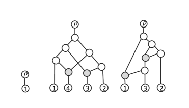
Figure 1: A phylogenetic network with a single leaf (left), a simplex network on 4 taxa and a tree-child network on 3 taxa that is not simplex (right), where reticulation nodes are represented by filled circles.

In this paper, we shall use the following facts frequently without mention of them.

Theorem 2.1.

Let $r(N)$, $\ell(N)$ denote the number of the reticulation nodes and leaves of a tree-child network $N$, respectively. Then,

1. $|{\cal T}(N)|=\ell(N)+r(N)-1$.

2. There are exactly $2\ell(N)+r(N)-1$ tree edges and $2r(N)$ reticulation edges in $N$.

2.2 Node depth, network height and Sackin index

Let $T$ be a phylogenetic tree and $u\in{\cal V}(T)\cup{\cal L}(T)$. The depth of $u$ is defined to be the number of edges in the unique path from the tree root $\rho$ to $u$, which is also equal to the number of ancestors of $u$. Obviously, the depth of the tree root is 0. The height of $T$ is defined to be the largest depth of a leaf in $T$.

In a phylogenetic network $N$, there are more than one path from the root $\rho$ to a specific descendant of a reticulation node. We generalize the concept of node depth to phylogenetic networks as follows.

Let $u$ be a node of $N$. The depth of a node $u$ is defined to be the number of edges in the longest path from the root $\rho$ to $u$, written as $d_{N}(u)$. The ancestor number of a node $u$ is defined to be the number of the ancestors of the node, written as $\alpha_{N}(u)$. For example, the depth and ancestral number of Leaf 4 are five are six, respectively, in the right phylogenetic network in Figure 2.

For a tree-child network $N$, we define the following parameters:

• The height of $N$ is defined to be the largest depth of a leaf, denoted by $h(N)$.

• The Sackin index of $N$ is defined to be the sum of the depths of its leaves, denoted by $K(N)$.

Given a family ${\cal F}$ of tree-child networks. The expected height of a network of the family ${\cal F}$ in the uniform model is defined by:

$$\overline{H}({\cal F})=\frac{1}{|{\cal F}|}\sum_{N\in{\cal F}}h(N),$$

where $|{\cal F}|$ is the cardinality of the set $\cal F$.

The expected Sackin index of a random network in ${\cal F}$ in the is defined by:

$$\overline{K}({\cal F})=\frac{1}{|{\cal F}|}\sum_{N\in{\cal F}}K(N).$$

Theorem 2.2.

Under the uniform model,

1. ([18]) The expected height of a random phylogenetic tree over $n$ taxa is asymptotically $2\sqrt{\pi n}$.

2. The expected Sackin index of a random phylogenetic tree on $n$ taxa is $\frac{2^{2n-2}n!(n-1)!}{(2n-2)!}$, whose is asymptotically $\sqrt{\pi}n^{3/2}$.

3 The expected Sackin index of random simplex networks

In this section, we will use an enumeration procedure and a simple counting formula for simplex networks that appear in [12] to obtain the asymptotic Sackin index of a simplex network in the uniform model.

3.1 Enumerating simplex networks

We first briefly introduce a procedure for enumerating simplex networks appearing in [12]. Let ${\cal OC}_{n}$ denote the class of simplex networks on $n$ taxa and $o_{n}=|{\cal OC}_{n}|$.

Let $N\in{\cal OC}_{n}$. $N$ contains It may contain 0 to $n-1$ reticulations. Recall that the child of each reticulation is a leaf. All the tree nodes and leaves that are not below any reticulations are connected to the root by tree edges, forming a connected subtree, which we call the top tree component and denote by $C(N)$ (see [7]). For instance, the top tree component of the simplex network in the middle of Figure 1 consists of Leaf 1, Leaf 4 and their ancestors, including $\rho$.

Let $[i,j]$ denote the integer set $\{i,i+1,\cdots,j\}$, where $0<i\leq j$. For any nonempty $I\subseteq[1,n]$, ${\cal OC}_{I,n}$ denotes the subset of simplex networks in which there are $n-|I|$ reticulations whose child are labeled uniquely with the elements of $[1,n]\setminus I$. Clearly, when $I=[1,n]$, ${\cal OC}_{I,n}$ is just the set of phylogenetic trees on $[1,n]$.

For simplicity, we write ${\cal OC}_{k,j}$ for ${\cal OC}_{[1,k],k+j}$ for $j>1$. The networks of ${\cal OC}_{k,j+1}$ can be generated by attaching the two grandparents of Leaf $j+1$ to each network $N$ of ${\cal OC}_{k,j}$ in the following two ways [12]:

1. For each tree edge $e=(u,v)$ of $C(N)$, where $u\not\in{\cal R}(N)$, subdivide $e$ into $(u,p),(p,q)$ and $(q,v)$, and add three new edges $(p,r),(q,r)$ and $(r,j+1)$, This insertion operation is shown on the left network in Figure 2, where $j+1=4$.

2. For each pair of tree edges $e^{\prime}=(u,v)$ and $e^{\prime\prime}=(s,t)$ of $C(N)$, i.e. $u\not\in{\cal R}(N)$ and $s\not\in{\cal R}(N)$, subdivide $e^{\prime}$ into $(u,p)$ and $(p,v)$ and $e^{\prime\prime}$ into $(s,q)$ and $(q,t)$, and add three new edges $(p,r),(q,r)$ and $(r,j+1)$. This insertion operation is shown in the right network in Figure 2.

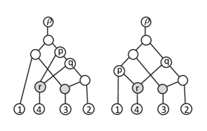
Figure 2: The Illustration of the procedure for enumerating simplex networks by attaching the grandparents ($p,q$) of a new leaf (4) below a reticulation node ($r$) onto either a tree edge (left) or a pair of tree edges (right) in the top tree component of a simplex network.

Each $N$ of ${\cal OC}_{k,j}$ contains exactly $2(k+j)-1$ tree edges in its $C(N)$. Additionally, all the networks generated using the above method are distinct [12]. This implies that $|{\cal OC}_{k,j+1}|=(2(k+j)-1)(k+j)|{\cal OC}_{k,j}|$ and thus

$$|{\cal OC}_{k,j}|=\frac{(2(k+j)-2)!}{2^{k+j-1}(k-1)!},$$ (1)

from which the simple formula for counting the phylogenetic trees is obtained by setting $j$ to 0.

By symmetry, ${\cal OC}_{I,n}={\cal OC}_{J,n}$ if $|I|=|J|$. Therefore, we obtain [12]:

$$o_{n}=\sum^{n}_{k=1}{n\choose k}|{\cal OC}_{k,n-k}|=\frac{(2n-2)!}{2^{n-1}}\sum^{n}_{k=0}{n\choose k}\frac{1}{(k-1)!}$$ (2)

3.2 A formula for the total depths of the nodes in the top tree component

Recall that $\alpha(u)$ denotes the number of ancestors of a node $u$. Let $\delta_{C(N)}(u)$ denote the number of descendants of $u$ that are in $C(N)$. We also use $\mbox{ToT}(N)$ to denote the tree edges of $C(N)$. We define:

$$A_{C}(N)=\sum_{v\in C(N)}\alpha_{N}(v)=\sum_{u\in C(N)}\delta_{C(N)}(u)$$ (3)

and

$$A_{C}({\cal OC}_{k,j})=\sum_{N\in{\cal OC}_{k,j}}A_{C}(N).$$ (4)

Lemma 3.1.

Assume $N\in{\cal OC}_{k,j}$ and let $n=k+j$. For each $e$ of $\mbox{\rm ToT}(N)$, we use $N(e)$ to denote the network obtained from $N$ by applying the first approach to $e$. Then,

$$\sum_{e\in ToT(N)}A_{C}(N(e))=(2n+3)A_{C}(N)+(2n-1)$$ (5)

Proof.

Let $e=(u,v)\in\mbox{ToT}(N)$. By the description of the first approach, the set of nodes and edges of $N(e)$ are respectively:

$${\cal V}(N(e))={\cal V}(N)\cup\{p,q,r,n+1\}$$

and

$${\cal E}(N(e))={\cal E}(N)\cup\{(u,p),(p,q),(q,v),(p,r),(q,r),(r,n+1)\}\setminus\{(u,v)\}$$

(see Figure 2).

Let ${\cal D}(v)$ be the set of descendants of $v$ in $C(N)$. We have the following facts:

$$|\alpha_{N(e)}(x)|=2+|\alpha_{N}(x)|, x\in{\cal D}(v)$$

$$|\alpha_{N(e)}(y)|=|\alpha_{N}(y)|, y\not\in{\cal D}_{N}(v)\cup\{v,p,q\}$$

$$|\alpha_{N(e)}(p)|=|\alpha_{N}(v)|,$$

$$|\alpha_{N(e)}(q)|=|\alpha_{N}(v)|+1,$$

$$|\alpha_{N(e)}(v)|=|\alpha_{N}(v)|+2.$$

Bu summing above equations, we obtain:

$$A_{C}(N(e))=A_{C}(N)+2\delta_{C(N)}(v)+2\alpha_{N}(v)+3.$$ (6)

Eqn. (3) and (6) imply that

$$\sum_{e\in\mbox{\scriptsize ToT}(N)}A_{C}(N(e))$$

$$= (2n-1)A_{C}(N)+2\sum_{(u,v)\in\mbox{\scriptsize ToT}(N)}\delta_{C(N)}(v)+2\sum_{(u,v)\in\mbox{\scriptsize ToT}(N)}\alpha_{N}(v)+3$$

$$= (2n-1)A_{C}(N)+2\left(\sum_{v\in C(N)}\delta_{C(N)}(v)-\delta_{C(N)}(\rho)\right)+2A_{C}(N)+3(2n-1)$$

$$= (2n+3)A_{C}(N)+(2n-1),$$

where $n=k+j$ and we use the fact that $\delta_{C(N)}(\rho)=2n-1$ for the network root $\rho$.

∎

Lemma 3.2.

Let $N\in{\cal OC}_{k,j}$ and $N(e^{\prime},e^{\prime\prime})$ denote the network obtained from $N$ using the second approach to a pair of distinct edges $e^{\prime},e^{\prime\prime}$ of $C(N)$. Then,

$$\sum_{\{e^{\prime},e^{\prime\prime}\}\subset ToT(N)}A_{C}(N(e^{\prime},e^{\prime\prime}))=(2n^{2}+n-2)A_{C}(N)-(2n-1),$$ (7)

where $n=k+j$.

Proof.

After attaching the reticulation node $r$ onto the edges $e^{\prime}=(u,v)$ and $e^{\prime\prime}=(s,t)$, the tree edge $e^{\prime}$ is divided into $e^{\prime}_{1}=(u,p)$ and $e^{\prime\prime}_{1}=(p,v)$; the edge $e^{\prime\prime}$ is divided into $e^{\prime}_{2}=(s,q)$ and $e^{\prime\prime}_{2}=(q,t)$, where $p,q$ are the parents of $r$ in $N(e^{\prime},e^{\prime\prime})$. We consider two possible cases.

First, we consider the case that $e^{\prime}\prec e^{\prime\prime}$. In $N(e^{\prime},e^{\prime\prime})$, for each descendant $x$ of $u$ in $C(N(e^{\prime},e^{\prime\prime})$ such that $x\neq p$ and $x$ is not below $s$, $\alpha(x)$ increases by 1 because of the subdivision of $e^{\prime}$. For each descendant $y$ of $s$ in $C(N(e^{\prime},e^{\prime\prime})$ such that $y\neq q$, $\alpha(y)$ increases by 2 because of the subdivision of $e^{\prime}$ and $e^{\prime\prime}$. Additionally,

$$\alpha_{N(e^{\prime},e^{\prime\prime})}(p)=\alpha_{N}(v)$$

and because $q$ is below $v$,

$$\alpha_{N(e^{\prime},e^{\prime\prime})}(q)=\alpha_{N}(t)+1.$$

For any tree node or leaves that are not the descendants of $u$, $\alpha(x)$ remains the same. Summing all together, we have that

$$A_{C}(N(e^{\prime},e^{\prime\prime}))=A_{C}(N)+\delta_{C(N)}(v)+\delta_{C(N)}(q)+\alpha_{N}(v)+\alpha_{N}(q)+3,$$ (8)

where 3 is the sum of the total increase of $\alpha(v)$, $\alpha(q)$ and $\alpha(t)$.

Summing over all the comparable edge pairs, we have

$$\sum_{e^{\prime},e^{\prime\prime}\in\mbox{\scriptsize ToT}(N):e^{\prime}\prec e^{\prime\prime}}A_{C}(N(e^{\prime},e^{\prime\prime}))$$ (9)

$$= (A_{C}(N)+3)|\{(e^{\prime},e^{\prime\prime})\;|\;e^{\prime}\prec e^{\prime\prime}\}|+\sum_{(u,v)\in\mbox{\scriptsize ToT}(N)}(\delta_{N}(v)+\alpha_{N}(v))\delta_{C(N)}(v)$$

$$+\sum_{(u,v)\in\mbox{\scriptsize ToT}(N)}(\delta_{C(N)}(v)+\alpha_{N}(v))(\alpha_{N}(v)-1)$$

$$= (A_{C}(N)+3)|\{(e^{\prime},e^{\prime\prime})\;|\;e^{\prime}\prec e^{\prime\prime}\}|+\sum_{v\in C(N)\setminus\{\rho\}}(\delta_{C(N)}(v)+\alpha_{N}(v))^{2}$$

$$-\sum_{v\in C(N)\setminus\{\rho\}}(\delta_{C(N)}(v)+\alpha_{N}(v))$$

$$= (A_{C}(N)+3)|\{(e^{\prime},e^{\prime\prime})\;|\;e^{\prime}\prec e^{\prime\prime}\}|+\sum_{v\in C(N)\setminus\{\rho\}}(\delta_{C(N)}(v)+\alpha_{N}(v))^{2}$$

$$-2A_{C}(N)+(2n-1),$$

where we use the fact that $\sum_{v\in C(N)\setminus\{\rho\}}\delta_{N}(v)=A_{C}(N)-(2n-1)$.

Second, we assume $e^{\prime}\|e^{\prime\prime}$. In $N(e^{\prime},e^{\prime\prime})$, for each descendant $x$ of $u$ in $C(N(e^{\prime},e^{\prime\prime}))$, $\alpha(x)$ increases by 1 because of the subdivision of $e^{\prime}$. For each descendant $y$ of $p$ in $C(N(e^{\prime},e^{\prime\prime}))$ , $\alpha(y)$ increases by 1 because of the subdivision of $e^{\prime\prime}$. Additionally, $\alpha_{N(e^{\prime},e^{\prime\prime})}(p)=\alpha_{N}(v)$ and $\alpha_{N(e^{\prime},e^{\prime\prime})}(q)=\alpha_{N}(t).$ For any tree node or leaves that are the descendants of neither $u$ nor $p$, $\alpha(x)$ remains the same. Hence,

$$A_{C}(N(e^{\prime},e^{\prime\prime}))=A_{C}(N)+\delta_{C(N)}(v)+\delta_{C(N)}(q)+\alpha_{N}(v)+\alpha_{N}(q)+2,$$ (10)

where $2$ counts for the increase by 1 of both $\alpha(v)$ and $\alpha(t)$.

Summing Eqn. (10) over parallel edge pairs, we obtain:

$$\sum_{e^{\prime},e^{\prime\prime}\in\mbox{\scriptsize ToT}(N):e^{\prime}\|e^{\prime\prime}}A_{C}(N(e^{\prime},e^{\prime\prime}))$$ (11)

$$= (A_{C}(N)+2)\left|\{(e^{\prime},e^{\prime\prime}):\;e^{\prime}\|e^{\prime\prime}\}\right|$$

$$+\sum_{(u,v)\in\mbox{\scriptsize ToT}(N)}o_{N}((u,v))(\delta_{C(N)}(v)+\alpha_{N}(v)),$$

where $o_{N}((u,v))$ is the number of the edges of $C(N)$ that are parallel to $(u,v)$.

Summing Eqn. (9) and (11) and using the facts that $n=k+j$ and $|\{(e^{\prime},e^{\prime\prime})\;|\;e^{\prime}\prec e^{\prime\prime}\}|=A_{C}(N)-(2n-1)$ and

$$\sum_{(u,v)\in\mbox{\scriptsize ToT}(N)}(\delta_{C(N)}(v)+\alpha_{N}(v))=2A_{C}(N)-\delta_{C(N)}(\rho)=2A_{C}(N)-(2n-1),$$

we obtain:

$$\sum_{\{e^{\prime},e^{\prime\prime}\}\subset ToT(N)}A_{C}(N(e^{\prime},e^{\prime\prime}))$$

$$= (A_{C}(N)+2){2n-1\choose 2}+|\{(e^{\prime},e^{\prime\prime})\;|\;e^{\prime}\prec e^{\prime\prime}\}|-2A_{C}(N)+(2n-1)$$

$$+(2n-1)\sum_{(u,v)\in\mbox{\scriptsize ToT}(N)}(\delta_{C(N)}(v)+\alpha_{N}(v))$$

$$= (A_{C}(N)+2){2n-1\choose 2}-A_{C}(N)+(2n-1)(2A_{C}(N)-(2n-1))$$

$$= A_{C}(N)(2n^{2}+n-2)-(2n-1).$$

∎

Theorem 3.1.

Let $k\geq 1$ and $j\geq 0$. For the subclass of simplex networks with $j$ reticulations whose children are $k+1,\cdots,k+j$ on $n=k+j$ taxa,

$$A_{C}({\cal OC}_{k,j})=\frac{(2n)!}{2^{j}(2k)!}\left(2^{k}k!-\frac{(2k-1)!}{2^{k-1}(k-1)!}\right).$$ (12)

Proof.

Summing Eqn. (5) and (7), we obtain

$$\sum_{e\in ToT(N)}A_{C}(N(e))+\sum_{\{e^{\prime},e^{\prime\prime}\}\subset ToT(N)}A_{C}(N(e^{\prime},e^{\prime\prime}))=(2n+1)(n+1)A_{C}(N)$$

for each $N\in{\cal OC}_{k,j}$. Summing the above equation over all networks of ${\cal TC}_{k,j}$, we have

$$A_{C}({\cal OC}_{k,j+1})=(2n+1)(n+1)\sum_{N\in{\cal OC}_{k,j}}A_{C}(N)=A_{C}({\cal OC}_{k,j})$$

or, equivalently, $A_{C}({\cal OC}_{k,j})=n(2n-1)A_{C}({\cal OC}_{k,j-1}).$ Since it is proved in [11] that

$$A_{C}({\cal OC}_{k,0})=2^{k}k!-\frac{(2k-1)!}{2^{k-1}(k-1)!},$$

we obtain Eqn. (12) by induction. ∎

3.3 The expected total c-depth of random simplex networks

The expected total c-depth of simplex networks with $j$ reticulations on $k+j$ leaves is defined as:

$$D_{C}(k,j)=\frac{{k+j\choose k}\sum_{N\in{\cal OC}_{k,j}}A_{C}(N)}{{k+j\choose k}|{\cal OC}_{k,j}|}=\frac{A_{C}({\cal OC}_{k,j})}{|{\cal OC}_{k,j}|}$$ (13)

in the uniform model. For each $n\geq 1$, the expected total c-depth of simplex networks on $n$ taxa becomes:

$$\overline{D}_{C}(n)=\left(\sum^{n}_{k=1}{n\choose k}A_{C}({\cal OC}_{k,n-k})\right)\mathbin{/}\left(\sum^{n}_{k=1}{n\choose k}|{\cal OC}_{k,n-k}|\right)$$ (14)

in the uniform model.

Proposition 3.1.

For any $k\geq 1$ and $j\geq 0$, the average total component depth $D_{C}(k,j)$ has the following asymptotic value.

$$D_{C}(k,j)=\frac{\sqrt{\pi}n(2n-1)}{\sqrt{k}}\left(1-\pi^{-1/2}k^{-1/2}+O(k^{-1})\right),$$ (15)

where $n=k+j$.

Proof.

Since ${2k\choose k}=\frac{2^{2k}}{\sqrt{\pi k}}(1-(8k)^{-1}+O(k^{-2})),$ by Eqn. (1),

$$D_{C}(k,j) = \frac{(2n)!}{2^{n-k}(2k)!}\left(2^{k}k!-\frac{(2k-1)!}{2^{k-1}(k-1)!}\right)/\left(\frac{(2n-2)!}{2^{n-1}(k-1)!}\right)$$

$$= \frac{n(2n-1)}{k}\left(\frac{2^{2k}k!k!}{(2k)!}-1\right)$$

$$= \frac{n(2n-1)}{k}\left(\frac{\sqrt{\pi k}}{1-(8k)^{-1}+O(k^{-2})}-1\right)$$

$$= \frac{\sqrt{\pi}n(2n-1)}{\sqrt{k}}\left(1-\frac{1}{\sqrt{\pi k}}+\frac{1}{8k}+O(k^{-2})\right).$$

Thus, Eqn. (15) is proved. ∎

Proposition 3.2.

For any $n>1$, $\overline{D}_{C}(n)$ has the following bounds.

$$(\sqrt{2}-1)(1+O(n^{-1/4}))\leq\frac{\overline{D}_{C}(n)}{\sqrt{\pi}n^{3/4}(2n-1)}\leq 2(1+O(n^{-1/4})).$$ (16)

Proof.

Let $S_{k}={n\choose k}|{\cal OC}_{k,n-k}|={n\choose k}\frac{(2n-2)!}{2^{n-1}(k-1)!}$ and $k_{0}=\sqrt{n+1}-1$.

By considering the ratio $S_{k+1}/S_{k}$, we can show (in Appendix A):

• $S_{k}\leq S_{k+1}$ for $k\in[1,k_{0}]$;

• $S_{k}>S_{k+1}$ if $k_{0}<k<2k_{0}$;

• $S_{k}>2S_{k+1}$ if $k\geq 2k_{0}$.

First, we define

$$f_{1}=\left(\sum_{k\leq k_{0}}D_{C}(k,n-k)S_{k}\right)\mathbin{/}\left(\sum_{k\leq k_{0}}S_{k}\right).$$

Since $D_{C}(k,n-k)$ is a decreasing function (which is proved in Appendix A),

$$f_{1}\geq D_{C}({\lfloor k_{0}\rfloor},n-{\lfloor k_{0}\rfloor})=\sqrt{\pi}n^{3/4}(2n-1)(1+O(n^{-1/4}))$$

Furthermore, since $S_{k}$ is increasing on $[1,k_{0})$,

$$f_{1} \leq \frac{1}{\lfloor k_{0}\rfloor}\sum_{k\leq\lfloor k_{0}\rfloor}D_{C}(k,n-k)$$

$$= \frac{\sqrt{\pi}n(2n-1)}{\lfloor k_{0}\rfloor}\sum_{k\leq\lfloor k_{0}\rfloor}\left(k^{-1/2}-\sqrt{\pi}k^{-1}+(1/8)k^{-3/2}+O(k^{-5/2}\right)$$

$$= \frac{\sqrt{\pi}n(2n-1)}{\lfloor k_{0}\rfloor}\left[2(\lfloor k_{0}\rfloor^{1/2}-1)-\sqrt{\pi}\ln\lfloor k_{0}\rfloor+O(\lfloor k_{0}\rfloor^{-1/2})\right]$$

$$= 2\sqrt{\pi}n^{3/4}(2n-1)(1+O(n^{-1/4}))$$

Second, define

$$f^{\prime}=\frac{\sum_{k\in[k_{0},2k_{0}]}D_{C}(k,n-k)S_{k}}{\sum_{k\in[k_{0},2k_{0}]}S_{k}}.$$ (17)

Since the $D_{C}(k,n-k)$ is a decreasing function and $S_{k}$ is decreasing on $[k_{0},2k_{0}]$,

$$f^{\prime}\leq D_{C}(\lceil k_{0}\rceil,n-\lfloor k_{0}\rfloor)=\sqrt{\pi}n^{3/4}(2n-1)(1+O(n^{-1/4}))$$

and, by Eqn. (15),

$$f^{\prime} \geq \frac{1}{k_{0}}\sum_{k\in[k_{0},2k_{0}]}D_{C}(k,n-k)$$

$$= \frac{\sqrt{\pi}n(2n-1)}{k_{0}}\sum_{k\in[k_{0},2k_{0}]}\left(k^{-1/2}-\sqrt{\pi}k^{-1}+(1/8)k^{-3/2}+O(k^{-5/2}\right)$$

$$= \frac{\sqrt{\pi}n(2n-1)}{k_{0}}\left[2(\sqrt{2}-1)k_{0}^{1/2}-\sqrt{\pi}\ln 2+(1/4)(1-\sqrt{1/2})k_{0}^{-1/2}+O(k_{0}^{-1})\right]$$

$$= 2(\sqrt{2}-1)\sqrt{\pi}n^{3/4}(2n-1)(1+O(n^{-1/4}))$$

Now, we consider

$$f_{2}=\frac{\sum_{k>k_{0}}D_{C}(k,n-k)S_{k}}{\sum_{k>k_{0}}S_{k}}.$$

For each $k>2k_{0}$, $D_{C}(k,n-k)\leq D_{C}(2k_{0},n-2k_{0})\leq f^{\prime}$. This implies that

$$\sum_{k>2k_{0}}D_{C}(k,n-k)S_{k}\leq f^{\prime}\sum_{k>2k_{0}}S_{k}$$

and thus

$$f_{2} = \frac{\sum_{k_{0}\leq k\leq 2k_{0}}D_{C}(k,n-k)S_{k}+\sum_{k>2k_{0}}D_{C}(k,n-k)S_{k}}{\sum_{k>k_{0}}S_{k}}$$

$$= \frac{f^{\prime}\sum_{k_{0}\leq k\leq 2k_{0}}S_{k}+\sum_{k>2k_{0}}D_{C}(k,n-k)S_{k}}{\sum_{k>k_{0}}S_{k}}$$

$$\leq \frac{f^{\prime}\sum_{k_{0}\leq k\leq 2k_{0}}S_{k}+f^{\prime}\sum_{k>2k_{0}}S_{k}}{\sum_{k>k_{0}}S_{k}}$$

$$= f^{\prime}$$

On the other hand, $S_{k}\geq 2S_{k+1}$ for $k\geq 2k_{0}$ and thus $\sum_{k>2k_{0}}S_{k}\leq 2S_{\lceil 2k_{0}\rceil}$

$$f_{2} \geq \frac{\sum_{k\in[k_{0},2k_{0}]}D_{C}(k,n-k)S_{k}}{\sum_{k>k_{0}}S_{k}}=\frac{f^{\prime}\sum_{k\in[k_{0},2k_{0}]}S_{k}}{\sum_{k\in[k_{0},2k_{0}]}S_{k}+\sum_{k>2k_{0}}S_{k}}$$

$$\geq \frac{f^{\prime}\sum_{k\in[k_{0},2k_{0}]}S_{k}}{2\sum_{k\in[k_{0},2k_{0}]}S_{k}}=f^{\prime}/2$$

The bounds on $f_{1}$ and $f_{2}$ implies that the mean value $f$ over the entire region is between $f_{1}$ and $f_{2}$, Thus we have proved that

$$(\sqrt{2}-1)\sqrt{\pi}n^{3/4}(2n-1)(1+O(n^{-1/4}))\leq\min(f^{\prime}/2,f_{1})\leq\overline{D}_{C}(n),$$

and

$$\overline{D}_{C}(n)\leq\max(f_{1},f_{2})\leq 2\sqrt{\pi}n^{3/4}(2n-1)(1+O(n^{-1/4})).$$

∎

3.4 Bounds on the Sackin index for random simplex network

Recall that $K(N)=\sum_{\ell\in{\cal L}(N)}d(\ell)$ for a network $N$.

Proposition 3.3.

For a simplex network $N\in{\cal OC}_{k,j}$,

$$K(N)\leq A_{C}(N)+1\leq 2K(N)$$

where $k\geq 1,j\geq 0$.

Proof.

Let $N\in{\cal OC}_{k,j}$. If $j=0$, $N$ does not contain any reticulation node and thus every node of $N$ is in the top tree component of $N$. By definition, $K(N)\leq A_{C}(N)$. Since $N$ is a phylogenetic tree, $N$ contains the same number of internal nodes (including the root $\rho$) as the number of leaves. By induction, we can prove that there exists a 1-to-1 mapping $\phi:{\cal T}(N)\cup\{\rho\}\rightarrow{\cal L}(N)$ such that $u$ is an ancestor of $\phi(u)$ for every $u$ (see Appendix B) Noting that $d_{N}(\rho)=0$ and $d_{N}(\phi(\rho))\geq 1$, we have:

$$A_{C}(N)+1\leq\sum_{\ell\in{\cal L}(N)}d_{N}(\ell)+\sum_{\ell\in{\cal T}(N)}d_{N}(\phi(u))=2K(N).$$

We now generalize the above proof for phylogenetic trees to the general case where $j>0$ as follows.

We assume that $r_{1},r_{2},\cdots,r_{j}$ are the $j$ reticulation nodes and their parents are $p^{\prime}_{j}$ and $p^{\prime\prime}_{j}$. Since $N$ is simplex, $p^{\prime}_{j}$ and $p^{\prime\prime}_{j}$ are both found in the top tree components. Clearly, $d_{N}(p^{\prime}_{j})\geq 1,d_{N}(p^{\prime\prime}_{j})\geq 1$. Since Leaf $(k+j)$ is the child of $r_{j}$, $d_{N}(k+j)=\max(d_{N}(p^{\prime}_{j}),d_{N}(p^{\prime\prime}_{j}))+2\leq d_{N}(p^{\prime}_{j})+d_{N}(p^{\prime\prime}_{j})$ unless $\min(d_{N}(p^{\prime}_{j}),d_{N}(p^{\prime\prime}_{j}))=1$.

If $d_{N}(p^{\prime}_{i})=\min(d_{N}(p^{\prime}_{i}),d_{N}(p^{\prime\prime}_{i}))=1$, $p^{\prime}_{i}$ is the unique child of the root $\rho$. This implies that $N$ contains at most an $i$ for which $\min(d_{N}(p^{\prime}_{i}),d_{N}(p^{\prime\prime}_{i}))=1$. Since $N$ is tree-child, the parents $p^{\prime}_{i}$ and $p^{\prime\prime}_{i}$ are distinct for different $i$, $K(N)\leq A_{C}(N)+1.$

Without loss of generality, we may further assume $d^{\prime}_{N}(p^{\prime}_{1})=1$. The tree-component $C(N)$ contains $k+2j$ internal tree nodes including $\rho$. We set

$${\cal T}(C(N))\setminus\{p^{\prime}_{i},p^{\prime\prime}_{i}:1\leq i\leq j\}=\{\rho,u_{1},\cdots,u_{k-1}\}.$$

Again, there is an 1-to-1 mapping $\phi$ from $\{\rho,u_{1},\cdots,u_{k-1}\}$ to ${\cal L}(C(N))=\{1,2,\cdots,k\}$ such that the leaf $\phi(u_{i})$ is a descendant of $u_{i}$. Therefore, since $d_{N}(\rho)=0$ and $d_{N}(\phi(\rho))\geq 1$,

$$d_{N}(\rho)+1 \leq d_{N}(\phi(\rho));$$

$$d_{N}(p^{\prime}_{i})+d_{N}(p^{\prime\prime}_{i}) \leq 2\max(d_{N}(p^{\prime}_{i}),d_{N}(p^{\prime\prime}_{i}))<2d_{N}(k+i),1\leq i\leq j;$$

$$d_{N}(u_{i})+d_{N}(\phi(u_{i})) \leq 2d_{N}(\phi(u_{i})),1\leq i\leq k-1.$$

Therefore, $A_{C}(N)+1\leq 2K(N).$ ∎

Theorem 3.2.

The expected Sackin index $\overline{K}({\cal OC}_{n})$ of a simplex network on $n$ taxa is $\Theta(n^{7/4})$.

Proof.

We define

$$K({\cal OC}_{k,j})=\sum_{N\in{\cal OC}_{k,j}}K(N),$$

where $k\geq 1$ and $j\geq 0$. By Proposition 3.3,

$$K({\cal OC}_{k,j})\leq A_{N}({\cal OC}_{k,j})+|{\cal OC}_{k,j}|\leq 2K({\cal OC}_{k,j}).$$

By Eqn. (16), we have:

$$\overline{K}({\cal OC}_{n}) = \frac{1}{\sum^{n}_{k=1}{n\choose k}|{\cal OC}_{k,n-k}|}\left(\sum^{n}_{k=1}{n\choose k}K\left({\cal OC}_{k,n-k}\right)\right)$$

$$\leq \frac{1}{\sum^{n}_{k=1}{n\choose k}|{\cal OC}_{k,n-k}|}\left(\sum^{n}_{k=1}{n\choose k}A_{C}\left({\cal OC}_{k,n-k}\right)\right)+1$$

$$= \overline{D}_{C}(n)+1$$

$$= 4\sqrt{\pi}n^{7/4}+1.$$

Similarly, using Eqn. (16), we have that

$$2\overline{K}({\cal OC}_{n})\geq\overline{D}_{C}(n)=2(\sqrt{2}-1)\sqrt{\pi}n^{7/4}+O(1),$$

equivalently,

$$\overline{K}({\cal OC}_{n})\geq(\sqrt{2}-1)\sqrt{\pi}n^{7/4}+O(1).$$

This concludes the proof. ∎

4 Conclusion

What facts about phylogenetic trees remain valid for phylogenetic networks is important in the study of phylogenetic networks. In this paper, an asymptotic estimate (up to constant ratio) for the expected Sackin index of a simplex network is given in the uniform model. This study raises a few research problems. First, the expected Sackin index of tree-child networks over $n$ taxa is still unknown. It is also interesting to investigate the Sackin index for galled trees, galled networks and other classes of networks (see [27] for example).

Secondly, it is even more challenging to estimate the expected height of simplex networks and tree-child networks. It is interesting to see whether or not the approach introduced by Stufler [19] can be used to answer this question.

Appendix

Appendix A

Proposition A.1. Let $S_{k}={n\choose k}\frac{(2n-2)!}{2^{n-1}(k-1)!}$ and $k_{0}=\sqrt{n+1}-1$. Then,

• $S_{k}\leq S_{k+1}$ for $k\in[1,k_{0}]$;

• $S_{k}>S_{k+1}$ if $k_{0}<k<2k_{0}$;

• $S_{k}>2S_{k+1}$ if $k\in[2k_{0},\infty)$.

Proof.

Note that

$$S_{k+1}=\frac{n-k}{k(k+1)}S_{k}.$$

If $k\leq k_{0}$, $(k+1)^{2}\leq(\sqrt{n+1}-1+1)^{2}=n+1$ and, equivalently, $k(1+k)\leq n-k$ and thus ${S_{k+1}}=\frac{n-k}{k(k+1)}S_{k}\geq S_{k}$. Similarly, ${S_{k+1}}<S_{k}$ if $k>k_{0}$.

If $k\geq 2k_{0}$, $(k+2)^{2}\geq 4(n+1)$ and $k^{2}+k\geq 4(n-k)+k\geq 4(n-k)$ and therefore, ${S_{k+1}}\leq\frac{1}{4}S_{k}<\frac{1}{2}S_{k}$. ∎

Proposition A.2. $D_{C}(k,n-k)$ is a decreasing function of $k$ on $[1,n-1]$.

Proof.

By Eqn. (1) and Eqn. (12),

$$D_{C}(k,n-k)=\frac{n(2n-1)}{k}\left(\frac{4^{k}k!k!}{(2k)!}-1\right).$$

Hence,

$$n(2n-1)[D_{C}(k,n-k)-D(k+1,n-k-1)]$$

$$= \frac{2^{2k}(k-1)!k!}{(2k)!}-\frac{2^{2k}4k!(k+1)!}{(2k+2)!}-\frac{1}{k(k+1)}$$

$$= \frac{2^{2k}k!(k-1)!}{(2k+1)!}-\frac{1}{k(k+1)}$$

$$= \frac{1}{k(k+1)}\left[\frac{2^{2k}k!(k+1)!}{(2k+1)!}-1\right]$$

$$= \frac{1}{k(k+1)}\left[\frac{4\times 6\times\cdots 2k\times(2k+2)}{3\times 5\times\cdots(2k+1)}-1\right]$$

$$> 0.$$

∎

Appendix B

Proposition B.1. Let $P$ be a phylogenetic tree on $n$ taxa. there exists a 1-to-1 mapping $\phi:{\cal T}(P)\cup\{\rho\}\rightarrow{\cal L}(P)$ such that $u$ is an ancestor of $\phi(u)$ for each $u\in{\cal T}(P)\cup\{\rho\}$.

Proof.

We prove the fact by mathematical induction on $n$. When $n=1$, we simply map the root $\rho$ to the only leaf.

Assume the fact is true for $n\leq k$, where $k\geq 1$. For a phylogenetic tree $P$ with $k+1$ leaves, we let the child of the root $\rho$ be $u$ and the two grandchildren be $v$ and $w$. We consider the subtree $P^{\prime}$ induced by $u$, $v$ and all the descendants of $v$ and the subtree $P^{\prime\prime}$ induced by $u$, $w$ and all the descendants of $w$.

Obviously, both $T^{\prime}$ and $T^{\prime\prime}$ have less than $k$ leaves. By induction, there is a 1-to-1 mapping $\phi^{\prime}:{\cal T}(P^{\prime})\cup\{u\}\rightarrow{\cal L}(P^{\prime})$ satisfying the constraints on leaves, and there is a 1-to-1 mapping $\phi^{\prime\prime}:{\cal T}(P^{\prime\prime})\cup\{u\}\rightarrow{\cal L}(P^{\prime\prime})$ satisfying the constraints on leaves. Let $\phi^{\prime}(u)=\ell$. Then, the function that maps $\rho$ to $\ell$, $u$ to $\phi^{\prime\prime}(u)$ and all the other tree nodes $x$ to $\phi^{\prime}(x)$ or $\phi^{\prime\prime}(x)$ depending whether it is in $P^{\prime}$ or $P^{\prime\prime}$. It is easy to verify that $\phi$ is a desired mapping. ∎

References

- [1] G. Cardona, F. Rosselló, G. Valiente, Comparison of Tree-Child Phylogenetic Networks, IEEE/ACM-TCBB 6 (4) (2009) 552–569. doi:10.1109/TCBB.2007.70270.
- [2] D. Gusfield, S. Eddhu, C. Langley, Efficient reconstruction of phylogenetic networks with constrained recombination, in: Proceedings of CSB’03, 2003.
- [3] D. H. Huson, T. H. Klöpper, Beyond galled trees - decomposition and computation of galled networks, in: Research in Computational Molecular Biology, 2007, pp. 211–225.
- [4] A. R. Francis, M. Steel, Which phylogenetic networks are merely trees with additional arcs?, Systematic Biology 64 (5) (2015) 768–777.
- [5] D. Gusfield, ReCombinatorics: The algorithmics of ancestral recombination graphs and explicit phylogenetic networks, MIT press, 2014.
- [6] D. H. Huson, R. Rupp, C. Scornavacca, Phylogenetic Networks: Concepts, Algorithms and Applications, Cambridge University Press, 2010.
- [7] A. D. Gunawan, B. DasGupta, L. Zhang, A decomposition theorem and two algorithms for reticulation-visible networks, Information and Computation 252 (2017) 161–175.
- [8] C. McDiarmid, C. Semple, D. Welsh, Counting phylogenetic networks, Annals of Combinatorics 19 (1) (2015) 205–224. doi:10.1007/s00026-015-0260-2.
- [9] M. Fuchs, G.-R. Yu, L. Zhang, On the asymptotic growth of the number of tree-child networks, European J. Combinatorics 93 (2021) 103278.
- [10] G. Cardona, J. C. Pons, C. Scornavacca, Generation of binary tree-child phylogenetic networks, PLoS Comput. Biology 15 (9) (2019) e1007347.
- [11] L. Zhang, Generating normal networks via leaf insertion and nearest neighbor interchange, BMC Bioinformatics 20 (20) (2019) 1–9.
- [12] G. Cardona, L. Zhang, Counting and enumerating tree-child networks and their subclasses, J. Comput. Syst. Sci. 114 (2020) 84–104.
- [13] M. Pons, J. Batle, Combinatorial characterization of a certain class of words and a conjectured connection with general subclasses of phylogenetic tree-child networks, Scientific Reports 11 (1) (2021) 1–14.
- [14] F. Bienvenu, A. Lambert, M. Steel, Combinatorial and stochastic properties of ranked tree-child networks, arXiv preprint arXiv:2007.09701 (2020).
- [15] M. Bouvel, P. Gambette, M. Mansouri, Counting phylogenetic networks of level 1 and 2, J. Math. Biology 81 (6) (2020) 1357–1395.
- [16] A. D. Gunawan, J. Rathin, L. Zhang, Counting and enumerating galled networks, Discrete Applied Math. 283 (2020) 644–654.
- [17] M. Fuchs, G.-R. Yu, L. Zhang, Asymptotic enumeration and distributional properties of galled networks, arXiv preprint arXiv:2010.13324 (2020).
- [18] P. Flajolet, A. Odlyzko, The average height of binary trees and other simple trees, J. Comput. Syst. Sci. 25 (2) (1982) 171–213.
- [19] B. Stufler, A branching process approach to level- phylogenetic networks, arXiv preprint arXiv:2102.10329 (2021).
- [20] M. J. Sackin, “good” and “bad” phenograms, Systematic Biology 21 (2) (1972) 225–226.
- [21] K.-T. Shao, R. R. Sokal, Tree balance, Systematic Zoology 39 (3) (1990) 266–276.
- [22] M. Avino, G. T. Ng, Y. He, M. S. Renaud, B. R. Jones, A. F. Poon, Tree shape-based approaches for the comparative study of cophylogeny, Ecology and Evolution 9 (12) (2019) 6756–6771.
- [23] C. Xue, Z. Liu, N. Goldenfeld, Scale-invariant topology and bursty branching of evolutionary trees emerge from niche construction, Proc. National Academy of Sciences 117 (14) (2020) 7879–7887.
- [24] M. Steel, Phylogeny: discrete and random processes in evolution, SIAM, 2016.
- [25] M. C. King, N. A. Rosenberg, A simple derivation of the mean of the sackin index of tree balance under the uniform model on rooted binary labeled trees, Math. Biosciences 342 (2021) 108688.
- [26] A. Mir, F. Rosselló, L. A. Rotger, A new balance index for phylogenetic trees, Math. Biosciences 241 (1) (2013) 125–136.
- [27] L. Zhang, Clusters, trees and phylogenetic network classes, in: T. Warnow (ed.): Bioinformatics and Phylogenetics –Seminal Contributions of Bernard Moret, Springer Nature, Switzerland, 2019, pp. 277–315.