Simulating Lindbladian evolution with non-abelian symmetries: Ballistic front propagation in the SU(2) Hubbard model with a localized loss

Abstract

We develop a non-Abelian time evolving block decimation (NA-TEBD) approach to study of open systems governed by Lindbladian time evolution, while exploiting an arbitrary number of abelian or non-abelian symmetries. We illustrate this method in a one-dimensional fermionic SU(2) Hubbard model on a semi-infinite lattice with localized particle loss at one end. We observe a ballistic front propagation with strongly renormalized front velocity, and a hydrodynamic current density profile. For large loss rates, a suppression of the particle current is observed, as a result of the quantum Zeno effect. Operator entanglement is found to propagate faster than the depletion profile, preceding the latter.

I Introduction

Understanding dynamical effects, correlations or entanglement properties in strongly correlated systems subject to dephasing or dissipation Harbola and Mukamel (2008); Breuer et al. (2016) or in systems under continuous monitoring Chin et al. (2010) represents a major challenge for modern condensed matter physics Müller et al. (2012). Recent experimental advances in ultracold atoms have made laboratory studies of the time dependent evolution of non-equilibrium states in such quantum many body systems possible Diehl et al. (2008); Schneider et al. (2012); Chong et al. (2018); Damanet et al. (2019). For example, quantum quenching the interaction by means of Freschbach resonances, has triggered enormous activity both experimentally Syassen et al. (2008); Cheneau et al. (2012); Barontini et al. (2013); Lapp et al. (2019) and theoretically Eckel et al. (2010); Calabrese et al. (2011); Buča and Prosen (2012); Eisert et al. (2015); Kormos et al. (2017); Mitra (2018). By now, state of the art experiments allow the study of the dynamics of even a single quantum level Fukuhara et al. (2013), or the implementation of microscopic spin filters in quantum point contact cold atom setups Lebrat et al. (2019). In some of these high resolution experiments the fundamental effect of measurement backaction due to an external observer becomes significant, and request a closer investigation of open many-body systems, where the interaction with the environment plays a major role.

A conceptually and mathematically consistent though computationally demanding approach to model the external environment in interacting systems is the Lindblad approach Wichterich et al. (2007); Prosen and Žnidarič (2012); Ajisaka et al. (2012a, b); Pižorn (2013); Karevski et al. (2013); Ajisaka et al. (2014); Arrigoni et al. (2013); Dorda et al. (2014, 2015); Jin et al. (2016); Schwarz et al. (2016). In the Lindbladian framework, time evolution is described in terms of the density operator, $\rho$, and the linear, hermiticity-preserving map $\cal L$, the so-called Lindbladian, which generates the time evolution of the density operator $\rho(t)$ via

$$i\,\dot{\rho} = {\cal L}[\,\rho\,]=[H,\rho]+{\cal D}\,[\,\rho\,]\,,$$ (1)

with the dissipator map, ${\cal D}=\sum_{F}\lambda_{F}\,{\cal D}_{F}$, written as a convex combination of elementary maps

$${\cal D}_{F}\,[\,\rho\,]\equiv i\,F\,\rho\,F^{\dagger}-{\textstyle{i\over 2}}\,\big{\{}\,F^{\dagger}F\,,\,\rho\,\big{\}}\,.$$ (2)

The Lindblad equation (1) describes the most general Markovian trace preserving dynamics, and generates a completely positive non-unitary map (a.k.a. quantum channel). The so-called Lindblad jump operators $F$ shall be later on simply referred to as dissipators.

Most of the numerical methods used to investigate time evolution, such as the time-evolving block decimation (TEBD)  Vidal (2003, 2004); Verstraete et al. (2004); Zwolak and Vidal (2004), the time dependent density matrix renormalization group (TD-DMRG)Daley et al. (2004); White and Feiguin (2004); Feiguin and White (2005) or time dependent variational principle (TDVP) Haegeman et al. (2013); Zauner-Stauber et al. (2018); Vanderstraeten et al. (2019) have been originally designed for closed systems. They are rarely used for open systems, where they request considerable computational effort and their use is therefore challenging Schollwöck (2005). In fact, already for such simple systems as the Hubbard chain, studied here, the dimension of the local space increases to $16$, which is extremely difficult to handle with standard matrix-product-state (MPS) methods. As we show here, efficient implementation of symmetries Werner et al. (2016); Hauschild and Pollmann (2018); Jaschke et al. (2018); Weichselbaum (2020) and, in particular, non-Abelian symmetries Werner et al. (2020), makes it possible to efficiently simulate the dissipative time evolution of these models.

Symmetry operations in quantum mechanics are represented by certain unitary (or antiunitary) operators, $U$, which transform quantum states into other quantum states, $|\psi\rangle\to|\psi_{U}\rangle\equiv U|\psi\rangle$. Similarly, $U$ transforms the density operator into another density operator, $\rho\to{\rho}_{U}=U\,\rho\,U^{\dagger}$. For closed systems, we call $U$ a symmetry if it commutes with the Hamiltonian, $[U,H]=0$, implying that time evolution commutes with the symmetry operation.We can easily extend this concept to open systems, where it entails the condition

$$U\,{\cal L}[\,\rho\,]\,U^{\dagger}={\cal L}[\,U\,\rho\,U^{\dagger}]\,.$$ (3)

Eq. (3) immediately implies that the time evolved density operator satisfies the relation, $\rho_{U}(t)=U\rho(t)U^{\dagger}$. As we show in Sections II and III, for non-Abelian symmetries, Eq. (3) has certain implications regarding the structure of the dissipator map: the groups of dissipators, $\{F_{m}\}$, related by symmetry transformations must occur with identical dissipation strength $\lambda_{F}$, otherwise they break the non-Abelian symmetry.

In this paper we further develop the notion of symmetries in the Liouville space — a vector space of density operators of the system, which allows us to handle abelian and non-abelian symmetries in a transparent and efficient way. Although non-abelian symmetries can be treated within the matrix product operator (MPO) approach,Werner et al. here we follow a technically somewhat simpler approach: we vectorize the density operator and the Lindblad equation Am-Shallem et al. (2015), and represent the vectorized density matrix as an MPS. We identify symmetry operations, and apply non-abelian MPS methods of Ref. Werner et al., 2020 in this augmented vector space.

Some lattice models with local losses have been studied earlier. Non-interacting fermions and bosons, e.g., have been analyzed in Refs Krapivsky et al., 2019 and Sels and Demler, 2020, respectively. Spinless fermions with nearest neighbor interactions Fröml et al. (2019, 2020); Wolff et al. (2020) or in Bose-Hubbard models Kepesidis and Hartmann (2012); Labouvie et al. (2016) have also been studied, however, spinful interacting models represent a major challenge due to the quickly increasing local operator space. The approach presented here allows us to investigate spinful fermion and boson models with matrix product methods efficiently, in cases where some non-abelian symmetry is not broken by dissipation.

We demonstrate the efficiency of our approach on the $SU(2)$ fermionic Hubbard model with localized particle loss at one end of the chain, and analyze the dynamics of various observables such as occupations and currents. This system, sketched in Fig. 1, can be relatively easily realized with ultracold atoms, by trapping fermions in an optical lattice, and using for example an electron beam Jaksch (2008); Barontini et al. (2013) to remove particles at one site. The Hubbard model is one of the simplest models that describes strongly interacting particles on a lattice. It is defined by the Hamiltonian,

$$H=-{J\over 2}\sum_{\sigma}\sum_{x=1}^{N-1}\big{(}c^{\dagger}_{x\sigma}c_{x+1\sigma}+h.c.\big{)}+U\sum_{x}n_{x\uparrow}n_{x\downarrow}\;,$$ (4)

where $c^{\dagger}_{x\sigma}$ creates a fermion at site $x$ with spin $\sigma$, $J$ denotes the hopping amplitude between nearest-neighboring sites, $U$ represents the interaction energy, and $n_{x\sigma}=c^{\dagger}_{x\sigma}c_{x\sigma}$ stands for the number operator at a given site. In the absence of dissipation or losses, the model belongs to the class of integrable models Lieb and Wu (1968); Ogata and Shiba (1990); Essler et al. (2005). To induce dissipation, we couple the first site to an external reservoir at time $t=0$, and induce particle loss there by the dissipators $F_{1\sigma}=c_{1\sigma}$. SU(2) symmetry then requires that the strength of the dissipators $F_{1\uparrow}$ and $F_{1\downarrow}$ be equal, $\lambda=\sqrt{\Gamma}$.

We perform TEBD simulations for this model, starting from an infinite temperature state, while benchmarking our numerical computations with exact third quantization results for the non-interacting case, $U=0$. The dissipator generates particle loss and a depletion region around itself, thereby inducing a depletion and current front, penetrating into the Hubbard chain. Surprisingly, both in the absence and in the presence of interactions, we observe ballistic front propagation. However, interactions renormalize the front velocity, and change the structure of the current profile and the spreading of the front dramatically.

Figure 1: Sketch of the one dimensional lattice. The two spin components of the electrons are represented by different colours. The hopping between nearest-neighbour sites is labeled by $J$, while the Coulomb on-site energy is represented by $U$. The first site in the chain is coupled to the external reservoir and has a dissipation rate $\Gamma$.

Our paper is organized as follows: In Sec. II we describe how the density matrix can be represented as an MPS by using the vectorization procedure. In Sec. II.1 we extend the concept of non-abelian symmetries to the Liouvillian evolution and construct the general non-abelian NA-MPS representation for the density matrix. In Sec. III we introduce the superfermion representation, which represents a practical and useful formalism that allows to construct a new set of creation and annihilation operators for the dual space. We use this formalism to construct the Liouvillian operator for the Hubbard chain with losses. In Sec. IV we demonstrate our approach on a semi-infinite SU(2) Hubbard chain with losses at one end, and present numerical results for various quantities of interest such as the average current or average density. In the non-interacting limit we compare these averages with the third quantization results. In Sec. V we sumarize the results and present the conclusions of our work. For completeness, we give in Appendix A details on the third quantization treatment of the free fermion case.

II MPS representation of the density matrix

TEBD is one of the leading approaches to simulate time dependent correlated systems subject to local interactions.Vidal (2003, 2004) It is best suited to one-dimensional lattice models with a tensor product Hilbert space structure,

$$\mathfrak{H}=\mathfrak{H}_{1}\otimes\mathfrak{H}_{2}\otimes\dots\otimes\mathfrak{H}_{N}\;,$$ (5)

where $\mathfrak{H}_{j}$ is the Hilbert space associated with a single site along the chain, and $N$ the length of the chain. Although it is not necessary, we assume for simplicity in what follows that all sites along the chain are identical and possess a Hilbert space of dimension $\dim(\mathfrak{H}_{j})=d$. We are interested in simulating the time evolution of an open system, described by the density matrix $\rho(t)$, the dynamics of which is dictated by the Lindblad equation,Lindblad (1976); Breuer and Petruccione (2002); Manzano (2020) Eq. (1).

The density matrix $\rho$ as well as other operators acting on $\mathfrak{H}$ are elements of an enlarged Hilbert space known as Liouville space Breuer and Petruccione (2002); Bolaños and Barberis-Blostein (2015), $\mathfrak{L}=\mathfrak{H}\otimes\mathfrak{H}^{*}$, where $\mathfrak{H}^{*}$ represents the dual (’bra’) Hilbert space with respect to $\mathfrak{H}$. Similar to (5), the Liouville space can be decomposed as a tensor product

$$\mathfrak{L}=\mathfrak{L}_{1}\otimes\mathfrak{L}_{2}\otimes\dots\otimes\mathfrak{L}_{N}\;,$$ (6)

and, by construction, the dimension $\dim(\mathfrak{L}_{j})=\dim(\mathfrak{H}_{j})^{2}=d^{2}$. The Liouville space of operators is endowed by a natural scalar product, $(a,b)\equiv\textrm{Tr}_{\mathfrak{H}}\{a^{\dagger}b\}$. Superoperators Breuer and Petruccione (2002) such as the Liouvillian or the dissipators are linear operators acting on $\mathfrak{L}$, and we denote them by calligraphic letters.

The vectorization, also termed as the Choi-Jamiolkowski isomorphism Dzhioev and Kosov (2011a); Jiang et al. (2013); Am-Shallem et al. (2015), is a basis dependent procedure, which allows us to treat the Liouville space and thus the space of density operators as a simple vector space. If $\{|\sigma_{x}\rangle\}$ is a local basis spanning the Hilbert space $\mathfrak{H}_{x}$, then the operators $|\sigma_{x}{\tilde{\sigma}}_{x})\equiv|\sigma_{x}\rangle\,\langle{\tilde{\sigma}}_{x}|$ form a basis in $\mathfrak{L}_{x}$,  and we can expand the density operator in this basis.

The Lindblad equation (1) is then transformed into a regular Schrödinger-like equation,

$$i\frac{d}{dt}|\rho)=\mathbb{L}|\rho)\,,$$ (7)

with $\it{\mathbb{L}}$ denoting the vectorized superoperator,

$$\mathbb{L} = H\otimes I-I\otimes H^{*}$$

$$+ i\,\textstyle{\sum_{F}}\,\lambda_{F}\,\big{\{}2F\otimes F^{*}-F^{\dagger}F\otimes I-I\otimes(F^{\dagger}F)^{*}\big{\}},$$

with $I$ the unit operator over $\mathfrak{H}$. Eq. (7) is then formally integrated as  

$$|\rho(t))=e^{-i\,\mathbb{L}\,t}|\rho(0))\,.$$ (9)

As long as the Hamiltonian $H$ and the dissipators $F$ are local, we can use the efficient methodology of matrix product states to generate the time evolution. In fact, similar to matrix product states, we can rewrite the state $|\rho)$ in an MPS form,

$$|\rho) = \sum_{a_{1},\dots a_{N-1}}\sum_{\sigma_{1},\dots\tilde{\sigma}_{L}}\mathcal{R}^{[1]\,a_{1}}_{(\sigma_{1}{\tilde{\sigma}}_{1})}\mathcal{R}^{[2]\,a_{2}}_{a_{1}(\sigma_{2}{\tilde{\sigma}}_{2})}\dots\mathcal{R}^{[N]}_{a_{N-1}(\sigma_{N}{\tilde{\sigma}}_{N})}\times$$ (10)

$$|\sigma_{1}{\tilde{\sigma}}_{1})\otimes|\sigma_{2}{\tilde{\sigma}}_{2})\otimes\dots\otimes|\sigma_{N}{\tilde{\sigma}}_{N})\;.$$

Notice that the evolution operator $\mathbb{V}(t)=e^{-i\,\mathbb{L}\,t}$ is non-Hermitian Ashida et al. (2020) due to dissipation introduced by the jump operators. Nevertheless, once $|\rho)$ is rewritten in this matrix product form, we can use the MPS machinery to generate the time evolution of $|\rho(t))$ within the TEBD approach,Zwolak and Vidal (2004); Verstraete et al. (2004) just as for unitary wave function evolution. As we mentioned in the introduction, the only problem arises due to dimensionality, since for just two fermionic degrees of freedom, the dimension of the local Liouville space $\mathfrak{L}$ is already 16. In the following, we shall reduce this number using non-Abelian symmetries down to 10, a number that can already be handled with standard desktop computers or work stations.

To summarize the notations, we shall use capital latin letters $A$, to label operators acting over the Hilbert space $\mathfrak{H}$. States in $\mathfrak{H}$ are denoted by the standard Dirac ket notation $|s\rangle$, with their Hermitian conjugates referred to as $\langle s|$. The complex conjugation of an operator $A$ with respect to computational basis is denoted as $A^{*}$. With calligraphic letters, e.g. $\cal{A}$, we denote superoperators acting over the Liouville space, $\mathfrak{L}$. Double-line letters, $\mathbb{A}$, denote operators acting on the vectorized Liouville space, while round kets $|\rho)$ denote states in the vectorized Lindblad space.

II.1 Symmetries in the Liouvillian approach

In this section, we extend the non-abelian TEBD (NA-TEBD) approach of Ref. Werner et al., 2020 to Lindbladian evolution and show that – with certain extensions – most concepts of Ref. Werner et al., 2020 remain applicable. In Hamiltonian systems, the symmetries are represented by a set of unitary (or antiunitary) transformations, $U(g)$, which leave the Hamiltonian invariant for all elements $g$ of the symmetry group $G$,

$$U(g)\,H\,U^{\dagger}(g)=H\,,\phantom{n}\textrm{ for}\phantom{n}\forall\,g\in G\;,$$ (11)

or, equivalently $U(g)H=H\,U(g)$. These symmetry operations are naturally extended to the Liouville space $\mathfrak{L}$ by the superoperator,

$${\cal U}(g)\;:\phantom{nn}\rho\phantom{n}\to\phantom{n}U(g)\,\rho\,U^{\dagger}(g)\;.$$ (12)

The superoperators ${\cal U}(g)$ thus represent a symmetry of the Liouvillian if

$${\cal U}(g)\,{\cal L}={\cal L}\,\,{\cal U}(g)\;,$$ (13)

written equivalently as Eq. (3), when applying both sides to an arbitrary density operator. Correspondingly, a generator $J$ of some continuous symmetry, $U=e^{i\phi J}$, is represented in Liouville space by a superoperator $\cal J$ as

$$J\phantom{n}\to\phantom{n}{\cal J}[\,\rho\,]\equiv J\,\rho-\rho\,J^{\dagger}\;,$$ (14)

where we now allowed complex parameters, $\phi$, and corresponding non-Hermitian generators.

Clearly, for Hamiltonian dynamics, ${\cal L}\to{\cal L}_{H}=[H\,,\,.\,]$, the condition (13), $[{\cal L}_{H},{\cal U}]=0$ and the familiar symmetry condition $[H\,,\,U]=0$ are equivalent. For open systems, however, $[{\cal L},{\cal U}]=0$ implies additional constraints on the structure of dissipators. Dissipators are operators, and as such, formally elements of the Liouville space, $F\in\mathfrak{L}$. Similar to states in the Hilbert space, the Liouville space of operators can be devided into irreducible subspaces of groups of irreducible tensor operators, $F_{q}$, which transform according to some irreducible representation of the symmetry group,

$${\cal U}(g)\,F_{q}={U(g)}\,F_{q}\,U(g)^{\dagger}=\sum_{q^{\prime}}\Gamma(g)^{q^{\prime}}_{q}\,F_{q^{\prime}}\;,$$ (15)

with $\Gamma(g)$ the representation of the group element, $g$. It is easy to show that the symmetry operation ${\cal U}$ commutes with the action of the dissipator under the condition that the strength of the dissipators belonging to the same irreducible representation is equal,

$${\cal D}\sim\lambda\sum_{q}{\cal D}_{F_{q}}\;.$$ (16)

This simple condition can also be naturally derived in case we construct the dissipator, as usual, from coupling the operators $F$ to some fluctuating fields, $\varphi_{F}$, and request that the subsystem and its environment be invariant under symmetry operations, as a composite system.

In the following, we shall assume that our dissipators satisfy Eq. (16), and focus furthermore on local symmetry operations, when $U(g)$ factorizes as

$$U(g)=U_{1}(g)\otimes U_{2}(g)\otimes\dots\otimes U_{N}(g)\;.$$ (17)

In this case, the Hilbert space can be decomposed into multiplets at each site

$$\mathfrak{H}_{j}=\mathrm{span}\left\{|\Gamma^{\rm local};\tau,\mu\rangle\right\}_{j}\;,$$ (18)

with index $\Gamma^{\rm local}$ denoting the irreducible representation, $\tau$ running over multiplets with a given representation, and $\mu$ labeling internal states of a multiplet. In general, if the model displays $n_{S}$ commuting symmetries, the label $\Gamma$ becomes a vector $\Gamma=(\Gamma_{1},\dots,\Gamma_{n_{S}})$, where $n_{S}$ is the total number of commuting symmetries. For the Hubbard model, studied here, e.g., we use spin SU(2) and charge U(1) symmetries, corresponding to $n_{S}=2$, and $\Gamma$ then refers to the corresponding spin and charge quantum numbers, $\Gamma\to(S,N)$. Having classified local states by symmetries, states in the Hilbert space $\mathfrak{H}$ can then be represented as non-Abelian matrix product statesWerner et al. (2020); Weichselbaum (2020) where the matrix product representation is decomposed into a trivial Clebsch-Gordan layer, and a non-trivial layer of reduced dimension, containing all necessary information.

This concept can be carried over to the Liouville space, while here we shall do that by implementing non-Abelian symmetries in vectorized space of operators. In the vectorized space, where the symmetry superoperator $\cal U$ is represented as ${\cal U}\to\mathbb{U}=U\otimes U^{*}$, while the symmetry generators become

$$\mathbb{J}=J\otimes I-I\otimes J^{*}\,.$$ (19)

Irreducible tensor operators $T_{q}$, as well as the dissipators $F_{q}$, are represented as states $T_{q}\to|T_{q})$, which then obey

$$\mathbb{U}(g)|T_{q})=\sum_{q^{\prime}}\Gamma(g)^{q^{\prime}}_{q}\,|T_{q^{\prime}})\;.$$ (20)

Similar to Eq. (18), the local vectorized Liouville space can be organized into ’operator multiplets’, $T^{[j]}_{q}$, represented in the local vectorized space as $|{\mathchoice{\raisebox{0.0pt}{\scalebox{1.0}[-1.0]{$\displaystyle\mathbb{L}$}}}{\raisebox{0.0pt}{\scalebox{1.0}[-1.0]{$\textstyle\mathbb{L}$}}}{\raisebox{0.0pt}{\scalebox{1.0}[-1.0]{$\scriptstyle\mathbb{L}$}}}{\raisebox{0.0pt}{\scalebox{1.0}[-1.0]{$\scriptscriptstyle\mathbb{L}$}}}}^{\rm loc};T,q)_{j}$, where we use the symbol $\textstyle\mathbb{L}$ to emphasize that these states belong to the vectorized Liouville space.

We can now extend the NA-TEBD approach to the vectorizes space and represent the density operator as a non-abelian MPS (NA-MPS) Werner et al. (2020)

$$|\rho)=\sum_{\left\{{\mathchoice{\raisebox{0.0pt}{\scalebox{1.0}[-1.0]{$\displaystyle\mathbb{L}$}}}{\raisebox{0.0pt}{\scalebox{1.0}[-1.0]{$\textstyle\mathbb{L}$}}}{\raisebox{0.0pt}{\scalebox{1.0}[-1.0]{$\scriptstyle\mathbb{L}$}}}{\raisebox{0.0pt}{\scalebox{1.0}[-1.0]{$\scriptscriptstyle\mathbb{L}$}}}}^{\mathrm{loc}}_{l}\right\}}\sum_{\left\{{\mathchoice{\raisebox{0.0pt}{\scalebox{1.0}[-1.0]{$\displaystyle\mathbb{L}$}}}{\raisebox{0.0pt}{\scalebox{1.0}[-1.0]{$\textstyle\mathbb{L}$}}}{\raisebox{0.0pt}{\scalebox{1.0}[-1.0]{$\scriptstyle\mathbb{L}$}}}{\raisebox{0.0pt}{\scalebox{1.0}[-1.0]{$\scriptscriptstyle\mathbb{L}$}}}}_{l}\right\}}\sum_{\left\{t_{l}\right\}}\sum_{\left\{T_{l}\right\}}\;\sum_{\left\{\alpha_{l}\right\}} R^{[1]}(\left\{{\mathchoice{\raisebox{0.0pt}{\scalebox{1.0}[-1.0]{$\displaystyle\mathbb{L}$}}}{\raisebox{0.0pt}{\scalebox{1.0}[-1.0]{$\textstyle\mathbb{L}$}}}{\raisebox{0.0pt}{\scalebox{1.0}[-1.0]{$\scriptstyle\mathbb{L}$}}}{\raisebox{0.0pt}{\scalebox{1.0}[-1.0]{$\scriptscriptstyle\mathbb{L}$}}}}\right\}^{[1]})_{T_{1}\,\alpha_{1}}^{t_{1}}\,R^{[2]}(\left\{{\mathchoice{\raisebox{0.0pt}{\scalebox{1.0}[-1.0]{$\displaystyle\mathbb{L}$}}}{\raisebox{0.0pt}{\scalebox{1.0}[-1.0]{$\textstyle\mathbb{L}$}}}{\raisebox{0.0pt}{\scalebox{1.0}[-1.0]{$\scriptstyle\mathbb{L}$}}}{\raisebox{0.0pt}{\scalebox{1.0}[-1.0]{$\scriptscriptstyle\mathbb{L}$}}}}\right\}^{[2]})_{t_{1}\,T_{2}\,\alpha_{2}}^{t_{2}}\,\dots\,R^{[N]}(\left\{{\mathchoice{\raisebox{0.0pt}{\scalebox{1.0}[-1.0]{$\displaystyle\mathbb{L}$}}}{\raisebox{0.0pt}{\scalebox{1.0}[-1.0]{$\textstyle\mathbb{L}$}}}{\raisebox{0.0pt}{\scalebox{1.0}[-1.0]{$\scriptstyle\mathbb{L}$}}}{\raisebox{0.0pt}{\scalebox{1.0}[-1.0]{$\scriptscriptstyle\mathbb{L}$}}}}\right\}^{[N]})_{t_{N-1}\,T_{N}\,\alpha_{N}}$$

$$\sum_{\left\{T_{l}\right\}}\sum_{\left\{Q_{l}\right\}} C(\left\{{\mathchoice{\raisebox{0.0pt}{\scalebox{1.0}[-1.0]{$\displaystyle\mathbb{L}$}}}{\raisebox{0.0pt}{\scalebox{1.0}[-1.0]{$\textstyle\mathbb{L}$}}}{\raisebox{0.0pt}{\scalebox{1.0}[-1.0]{$\scriptstyle\mathbb{L}$}}}{\raisebox{0.0pt}{\scalebox{1.0}[-1.0]{$\scriptscriptstyle\mathbb{L}$}}}}\right\}^{[1]})_{0\,q_{1}}^{p_{1},\,\alpha_{1}}\,C(\left\{{\mathchoice{\raisebox{0.0pt}{\scalebox{1.0}[-1.0]{$\displaystyle\mathbb{L}$}}}{\raisebox{0.0pt}{\scalebox{1.0}[-1.0]{$\textstyle\mathbb{L}$}}}{\raisebox{0.0pt}{\scalebox{1.0}[-1.0]{$\scriptstyle\mathbb{L}$}}}{\raisebox{0.0pt}{\scalebox{1.0}[-1.0]{$\scriptscriptstyle\mathbb{L}$}}}}\right\}^{[2]})_{p_{1}\,q_{2}}^{p_{2},\,\alpha_{2}}\,\dots\,C(\left\{{\mathchoice{\raisebox{0.0pt}{\scalebox{1.0}[-1.0]{$\displaystyle\mathbb{L}$}}}{\raisebox{0.0pt}{\scalebox{1.0}[-1.0]{$\textstyle\mathbb{L}$}}}{\raisebox{0.0pt}{\scalebox{1.0}[-1.0]{$\scriptstyle\mathbb{L}$}}}{\raisebox{0.0pt}{\scalebox{1.0}[-1.0]{$\scriptscriptstyle\mathbb{L}$}}}}\right\}^{[N]})_{p_{N-1}\,q_{N}}^{0,\,\alpha_{N}}$$ (21)

$$|{\mathchoice{\raisebox{0.0pt}{\scalebox{1.0}[-1.0]{$\displaystyle\mathbb{L}$}}}{\raisebox{0.0pt}{\scalebox{1.0}[-1.0]{$\textstyle\mathbb{L}$}}}{\raisebox{0.0pt}{\scalebox{1.0}[-1.0]{$\scriptstyle\mathbb{L}$}}}{\raisebox{0.0pt}{\scalebox{1.0}[-1.0]{$\scriptscriptstyle\mathbb{L}$}}}}^{\mathrm{loc}}_{1};T_{1},q_{1})\otimes|{\mathchoice{\raisebox{0.0pt}{\scalebox{1.0}[-1.0]{$\displaystyle\mathbb{L}$}}}{\raisebox{0.0pt}{\scalebox{1.0}[-1.0]{$\textstyle\mathbb{L}$}}}{\raisebox{0.0pt}{\scalebox{1.0}[-1.0]{$\scriptstyle\mathbb{L}$}}}{\raisebox{0.0pt}{\scalebox{1.0}[-1.0]{$\scriptscriptstyle\mathbb{L}$}}}}^{\mathrm{loc}}_{2};T_{2},q_{2})\otimes\dots\otimes|{\mathchoice{\raisebox{0.0pt}{\scalebox{1.0}[-1.0]{$\displaystyle\mathbb{L}$}}}{\raisebox{0.0pt}{\scalebox{1.0}[-1.0]{$\textstyle\mathbb{L}$}}}{\raisebox{0.0pt}{\scalebox{1.0}[-1.0]{$\scriptstyle\mathbb{L}$}}}{\raisebox{0.0pt}{\scalebox{1.0}[-1.0]{$\scriptscriptstyle\mathbb{L}$}}}}^{\mathrm{loc}}_{N};T_{N},q_{N})\;.$$

In our construction, the NA-MPS structure has two layers (see Fig. 2). The upper layer contains the tensors $R^{[x]}(\left\{{\mathchoice{\raisebox{0.0pt}{\scalebox{1.0}[-1.0]{$\displaystyle\mathbb{L}$}}}{\raisebox{0.0pt}{\scalebox{1.0}[-1.0]{$\textstyle\mathbb{L}$}}}{\raisebox{0.0pt}{\scalebox{1.0}[-1.0]{$\scriptstyle\mathbb{L}$}}}{\raisebox{0.0pt}{\scalebox{1.0}[-1.0]{$\scriptscriptstyle\mathbb{L}$}}}}\right\}^{[x]})^{t_{x}}_{t_{x-1}\,T_{x}\,\alpha_{x}}$, which carry the essential information of the state, while the lower layer includes exclusively Clebsch-Gordon coefficients, $C(\left\{{\mathchoice{\raisebox{0.0pt}{\scalebox{1.0}[-1.0]{$\displaystyle\mathbb{L}$}}}{\raisebox{0.0pt}{\scalebox{1.0}[-1.0]{$\textstyle\mathbb{L}$}}}{\raisebox{0.0pt}{\scalebox{1.0}[-1.0]{$\scriptstyle\mathbb{L}$}}}{\raisebox{0.0pt}{\scalebox{1.0}[-1.0]{$\scriptscriptstyle\mathbb{L}$}}}}\right\}^{[x]})_{p_{x-1}\,q_{x}}^{p_{x}\,\alpha_{x}}$, and carries all the symmetry-related ’trivial’ information.Werner et al. (2020) In Eq. (II.1) we used a compact notation for the set of irreducible representation labels, $\left\{{\mathchoice{\raisebox{0.0pt}{\scalebox{1.0}[-1.0]{$\displaystyle\mathbb{L}$}}}{\raisebox{0.0pt}{\scalebox{1.0}[-1.0]{$\textstyle\mathbb{L}$}}}{\raisebox{0.0pt}{\scalebox{1.0}[-1.0]{$\scriptstyle\mathbb{L}$}}}{\raisebox{0.0pt}{\scalebox{1.0}[-1.0]{$\scriptscriptstyle\mathbb{L}$}}}}\right\}^{[x]}=({\mathchoice{\raisebox{0.0pt}{\scalebox{1.0}[-1.0]{$\displaystyle\mathbb{L}$}}}{\raisebox{0.0pt}{\scalebox{1.0}[-1.0]{$\textstyle\mathbb{L}$}}}{\raisebox{0.0pt}{\scalebox{1.0}[-1.0]{$\scriptstyle\mathbb{L}$}}}{\raisebox{0.0pt}{\scalebox{1.0}[-1.0]{$\scriptscriptstyle\mathbb{L}$}}}}_{x-1},{\mathchoice{\raisebox{0.0pt}{\scalebox{1.0}[-1.0]{$\displaystyle\mathbb{L}$}}}{\raisebox{0.0pt}{\scalebox{1.0}[-1.0]{$\textstyle\mathbb{L}$}}}{\raisebox{0.0pt}{\scalebox{1.0}[-1.0]{$\scriptstyle\mathbb{L}$}}}{\raisebox{0.0pt}{\scalebox{1.0}[-1.0]{$\scriptscriptstyle\mathbb{L}$}}}}^{\mathrm{loc}}_{x},{\mathchoice{\raisebox{0.0pt}{\scalebox{1.0}[-1.0]{$\displaystyle\mathbb{L}$}}}{\raisebox{0.0pt}{\scalebox{1.0}[-1.0]{$\textstyle\mathbb{L}$}}}{\raisebox{0.0pt}{\scalebox{1.0}[-1.0]{$\scriptstyle\mathbb{L}$}}}{\raisebox{0.0pt}{\scalebox{1.0}[-1.0]{$\scriptscriptstyle\mathbb{L}$}}}}_{x})$, associated with the legs of the tensors $R^{[x]}$. The index $\alpha_{l}$ represents the outer-multiplicity label, and depends in general on $\left\{{\mathchoice{\raisebox{0.0pt}{\scalebox{1.0}[-1.0]{$\displaystyle\mathbb{L}$}}}{\raisebox{0.0pt}{\scalebox{1.0}[-1.0]{$\textstyle\mathbb{L}$}}}{\raisebox{0.0pt}{\scalebox{1.0}[-1.0]{$\scriptstyle\mathbb{L}$}}}{\raisebox{0.0pt}{\scalebox{1.0}[-1.0]{$\scriptscriptstyle\mathbb{L}$}}}}\right\}^{[x]}$. This NA-MPS structure naturally incorporates abelian symmetries as well. Then Clebsch-Gordan coefficients are just 1 for representation labels ${{\mathchoice{\raisebox{0.0pt}{\scalebox{1.0}[-1.0]{$\displaystyle\mathbb{L}$}}}{\raisebox{0.0pt}{\scalebox{1.0}[-1.0]{$\textstyle\mathbb{L}$}}}{\raisebox{0.0pt}{\scalebox{1.0}[-1.0]{$\scriptstyle\mathbb{L}$}}}{\raisebox{0.0pt}{\scalebox{1.0}[-1.0]{$\scriptscriptstyle\mathbb{L}$}}}}}^{[x]}$ allowed by the selection rules.

In case of local dissipators and a local Hamiltonian containing only nearest neighbor interactions and hopping, we can now proceed just as in Ref. Werner et al., 2020, and ’Trotterize’ the (vectorized) evolution operator, $\mathbb{V}=e^{-i\,t\,\mathbb{L}}$, and eliminate the Clebsch-Gordan layer.Werner et al. (2020) TEBD or DMRG steps can then be carried out very efficiently, by carrying out the singular value decompositions in separate symmetry sectors independently.

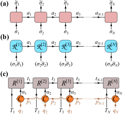
Figure 2: (a) MPO representation of a general density matrix. (b) Merging the legs of the MPO allows us to represent the density matrix as an MPS. (c) Graphical representation of the NA-MPS in equation (II.1). The NA-MPS tensor consists of two layers. The upper layer is the ’core’ NA-MPS, while the lower layer is built from Clebsch-Gordan coefficients and carries all symmetry-related information.

III Vectorization: superfermion representation

We now vectorize the Liouvillan space using the so-called superfermion representation,Dzhioev and Kosov (2011a, b, 2012) which introduces a new set of creation/annihilation operators $\tilde{c}_{j\sigma}$ acting in the dual Fock space. These operators satisfy the usual anticommutation relations, $\{\tilde{c}_{j\sigma},\tilde{c}^{\dagger}_{k\sigma^{\prime}}\}=\delta_{jk}\delta_{\sigma\sigma^{\prime}}$, etc. The operators $c_{j\sigma}^{(\dagger)}$ and $\tilde{c}^{(\dagger)}_{k\sigma^{\prime}}$ act nontrivially on different Fock spaces, and also anticommute, $\{c_{j\sigma},\tilde{c}^{(\dagger)}_{k\sigma^{\prime}}\}=0$. In this formalism the vectorized Liouvillian (II) becomes

$$\mathbb{L} = -{J\over 2}\sum_{\sigma}\sum_{i=1}^{L-1}\big{(}c^{\dagger}_{i\sigma}c_{i+1\sigma}+h.c.\big{)}+U\sum_{i}n_{i\uparrow}n_{i\downarrow}\;$$ (22)

$$+ {J\over 2}\sum_{\sigma}\sum_{i=1}^{L-1}\big{(}\tilde{c}^{\dagger}_{i\sigma}\tilde{c}_{i+1\sigma}+h.c.\big{)}-U\sum_{i}\tilde{n}_{i\uparrow}\tilde{n}_{i\downarrow}$$

$$+ 2i\Gamma\sum_{\sigma}c_{1\sigma}\tilde{c}_{1\sigma}-i\Gamma\sum_{\sigma}\big{(}\tilde{c}^{\dagger}_{1\sigma}\tilde{c}_{1\sigma}-c^{\dagger}_{1\sigma}c_{1\sigma}\big{)}\,.$$

Here we follow a general approach, and form the local tensor product space by acting with the $c_{i}^{(\dagger)}$ and $\tilde{c}^{(\dagger)}_{i}$ operators. In the specific case studied here, however, we may consider regarding the Liouvillian Eq. (22) as a non-Hermitian Hamiltonian for a two-chain (ladder) model coupled via the first site, and construct an MPS representation by separating the sites and ordering the dual operators $\tilde{c}^{(\dagger)}_{i}$ to act on the sites $i=-N+1,-N+2,\dots,0$, while the regular operators $c_{i}^{(\dagger)}$ act on the sites $i=1,2\dots N-1,N$ along the chain. In this way, we would double the length of the chain and the tilde and the regular sites are coupled at the center of the chain. The price we would pay, however, is that even an infinite temperature initial state would contain long-ranged entanglement. Moreover, in the general case of more local dissipators along the chain, dissipators would induce long-ranged terms in the effective Hamiltonian, causing additional difficulties. In contrast, within the tensor product state approach we follow, the size of the local space is larger, but the initial state has a simple structure, dissipators remain local, and the chain is half as long as in the unfolded chain approach.

The vectorized Liouvillan, Eq. (22) then acts on the Fock space of vectorized operators, i.e., the vectorized Liouville space. To propagate the vectorized Linblad equation, Eq. (9), we thus need to represent the density matrix $|\rho(t))$ within the superfermions’ Fock space, and then follow the regular TEBD approach, generated by Eq. (22).

Let us now elaborate on the symmetries of the Hamiltonian Eq. (4) and their representation on the Liouville space. The spin operator ${\bf S}={1\over 2}\sum_{i,\sigma\sigma^{\prime}}c^{\dagger}_{i\sigma}\boldsymbol{\sigma}_{\sigma\sigma^{\prime}}c_{i\sigma^{\prime}}$ as well as the normal ordered total charge $N=\sum_{i,\sigma}(c^{\dagger}_{i\sigma}c_{i\sigma}-1)$ commute with $H$ in (4), which thus displays a $G=SU(2)\otimes U(1)$ symmetry. Accordingly, local states in the Hilbert space $\mathfrak{H}^{\mathrm{loc}}$ can be classified by spin and charge quantum numbers, $\Gamma^{\mathrm{loc}}=(S^{\mathrm{loc}},N^{\mathrm{loc}})$.

To carry out a similar classification in the local, vectorized Liouville space, we must represent first symmetry operations acting on this space, as outlined earlier. Spin rotations, e.g., are generated by the operators

$$\mathbb{S}_{j}^{\alpha}=S_{j}^{\alpha}\otimes I-I\otimes{S_{j}^{\alpha}}^{*}\,,\phantom{aaa}(\alpha=x,y,z)\;.$$

Similarly, $U(1)$ gauge transformations are generated by $\mathbb{N}_{j}=N_{j}\otimes I-I\otimes{N_{j}}$ in the vectorized space. Notice that the ’raising operator’ $\mathbb{S}^{+}$ becomes $\mathbb{S}^{+}=\mathbb{S}^{x}+i\,\mathbb{S}^{y}=S^{+}\otimes I-I\otimes{S^{-}}$ when acting over the vectorized space.

We can easily represent the operators $\mathbb{S}^{\pm}$ and $\mathbb{S}^{z}$ in the superfermion representation by using the operators $c_{j\sigma}$ and $\tilde{c}_{j\sigma}$ asDzhioev and Kosov (2011a, b)

$$\ {\mathbb{S}^{+}_{j}} = c^{\dagger}_{j\uparrow}c_{j\downarrow}-\tilde{c}^{\dagger}_{j\downarrow}\tilde{c}_{j\uparrow}\;,$$ (23)

$${\mathbb{S}}^{z}_{j} = {1\over 2}\big{(}c^{\dagger}_{j\uparrow}c_{j\uparrow}-c^{\dagger}_{j\downarrow}c_{j\downarrow}\big{)}-{1\over 2}\big{(}\tilde{c}^{\dagger}_{j\uparrow}\tilde{c}_{j\uparrow}-\tilde{c}^{\dagger}_{j\downarrow}\tilde{c}_{j\downarrow}\big{)}\;,$$

$${\mathbb{S}^{-}_{j}} = c^{\dagger}_{j\uparrow}c_{j\downarrow}-\tilde{c}^{\dagger}_{j\downarrow}\tilde{c}_{j\uparrow}\;.$$

In a similar way, the U(1) symmetry related to particle conservation is generated by

$$\mathbb{N}_{j}=\sum_{\sigma}(c^{\dagger}_{j\sigma}c_{j\sigma}-\tilde{c}^{\dagger}_{j\sigma}\tilde{c}_{j\sigma})\,.$$ (24)

Having identified the symmetry generators over the vectorized Liouville space, we can now identify families irreducible tensor operators. In the local Liouville space, $\mathfrak{L}_{j}$ at site $j$, e.g., the spin operators $-S_{j}^{+}/\sqrt{2}$, $S^{z}$, $S_{j}^{-}/\sqrt{2}$, form the three components of a spin ${\cal S}=1$ vector operator of charge ${\cal N}=0$. Similarly, the creation operators are $c^{\dagger}_{j}=(c^{\dagger}_{j\uparrow},c^{\dagger}_{j\downarrow})$ and the annihilation operators $\tilde{c}_{j}=(\tilde{c}_{j\uparrow},-\tilde{c}_{j\downarrow})$ are spin ${\cal S}=1/2$ operators of charge ${\cal N}=1$ and ${\cal N}=-1$, respectively.

${\mathchoice{\raisebox{0.0pt}{\scalebox{1.0}[-1.0]{$\displaystyle\mathbb{L}$}}}{\raisebox{0.0pt}{\scalebox{1.0}[-1.0]{$\textstyle\mathbb{L}$}}}{\raisebox{0.0pt}{\scalebox{1.0}[-1.0]{$\scriptstyle\mathbb{L}$}}}{\raisebox{0.0pt}{\scalebox{1.0}[-1.0]{$\scriptscriptstyle\mathbb{L}$}}}}=(\mathbb{S},\;\mathbb{N})$	$\dim({\mathchoice{\raisebox{0.0pt}{\scalebox{1.0}[-1.0]{$\displaystyle\mathbb{L}$}}}{\raisebox{0.0pt}{\scalebox{1.0}[-1.0]{$\textstyle\mathbb{L}$}}}{\raisebox{0.0pt}{\scalebox{1.0}[-1.0]{$\scriptstyle\mathbb{L}$}}}{\raisebox{0.0pt}{\scalebox{1.0}[-1.0]{$\scriptscriptstyle\mathbb{L}$}}}})$	$T$	states
(0, -2)	1	1	$\tilde{c}^{\dagger}_{\uparrow}\tilde{c}^{\dagger}_{\downarrow}|0)$
(0, 0)	1	1	$|0)$
		2	${1\over\sqrt{2}}(c^{\dagger}_{\uparrow}\tilde{c}^{\dagger}_{\uparrow}-c^{\dagger}_{\downarrow}\tilde{c}^{\dagger}_{\downarrow})|0)$
		3	$c^{\dagger}_{\uparrow}c^{\dagger}_{\downarrow}\tilde{c}^{\dagger}_{\uparrow}\tilde{c}^{\dagger}_{\downarrow}|0)$
(0,  2)	1	1	$c^{\dagger}_{\uparrow}c^{\dagger}_{\downarrow}|0)$
(${1\over 2}$, -1)	2	1	$\big{\{}\tilde{c}^{\dagger}_{\uparrow}|0)$, $\tilde{c}^{\dagger}_{\downarrow}|0)\big{\}}$
		2	$\big{\{}c^{\dagger}_{\uparrow}\tilde{c}^{\dagger}_{\uparrow}\tilde{c}^{\dagger}_{\downarrow}|0)$, $c^{\dagger}_{\downarrow}\tilde{c}^{\dagger}_{\uparrow}\tilde{c}^{\dagger}_{\downarrow}|0)\big{\}}$
(${1\over 2}$ ; 1)	2	1	$\big{\{}c^{\dagger}_{\uparrow}|0)$, $c^{\dagger}_{\downarrow}|0)\big{\}}$
		2	$\big{\{}c^{\dagger}_{\uparrow}c^{\dagger}_{\downarrow}\tilde{c}^{\dagger}_{\downarrow}|0)$, $c^{\dagger}_{\uparrow}c^{\dagger}_{\downarrow}\tilde{c}^{\dagger}_{\uparrow}|0)\big{\}}$
			$\big{\{}\;c^{\dagger}_{\downarrow}\tilde{c}^{\dagger}_{\uparrow}|0)$
(1, 0)	3	1	${1\over\sqrt{2}}(c^{\dagger}_{\uparrow}\tilde{c}^{\dagger}_{\uparrow}+c^{\dagger}_{\downarrow}\tilde{c}^{\dagger}_{\downarrow})|0)$
			$c^{\dagger}_{\uparrow}\tilde{c}^{\dagger}_{\downarrow}|0)\;\big{\}}$

Table 1: $SU(2)$ multiplets as they are indexed by the quantum numbers for the total spin $\mathbb{S}$ and occupation $\mathbb{N}$.

In the vectorized form, all these operators of the Liouville space $\mathfrak{L}_{j}$ are represented as Fock states. The spin operator $S^{+}_{j}\in\mathfrak{L}_{j}$ is identified, e.g., by the state $|S^{+}_{j})=c^{\dagger}_{j\uparrow}\tilde{c}^{\dagger}_{j\downarrow}|0)$. The $4\times 4=16$ local operators are then represented by 16 Fock states, listed in Table 1, which can then be organized into 6 symmetry sectors, and altogether 10 multiplets.

Notice that, although the Lindbladian dissipator removes particles, the Lindbladian $U(1)$ charge ${\cal N}$ (or $\mathbb{N}$ in the vectorized form) is conserved. This can be verified directly by investigating the condition (3), or by looking at the commutator of Eqs. (24) and (22). We can thus use the fulll $SU(2)\times U(1)$ weak Liouvillian symmetry, even though the total charge is not conserved.

IV Application to the SU(2) Hubbard model

In this section, we demonstrate our approach on the semi-infinite fermionic SU(2) Hubbard model with a particle sink at the end of the chain. We execute a ’dissipation quench’: we start our simulations by constructing a half-filled infinite temperature state, which can be created relatively simply in cold atom experiments,Braun et al. (2013); Tarruell and Sanchez-Palencia (2018) and turn on a ’particle sink’ process at site $0$ at time $t=0$. The sink empties the semi-infinite chain, thereby creating a moving front between the emptied and occupied regions, and the quantum-mechaical time evolution generating entanglement.

In the vectorized formalism, the infinite temperature half-filled initial state translates to the state

$$|\rho(0))=\prod_{x=1}^{N}\frac{1+c^{\dagger}_{x\uparrow}c^{\dagger}_{x\downarrow}\tilde{c}^{\dagger}_{x\uparrow}\tilde{c}^{\dagger}_{x\downarrow}+c^{\dagger}_{x\uparrow}\tilde{c}^{\dagger}_{x\uparrow}+c^{\dagger}_{x\downarrow}\tilde{c}^{\dagger}_{x\downarrow}}{2}\;|0)\,.$$ (25)

Being the product of local states, this vectorized state has a trivial MPS representation, and possesses Liouvillian quantum numbers ${\cal S}=0$, and ${\cal N}=0$, implying that $|\rho(0))$ is an SU(2) super-singlet.

To compute time dependent observables, we simply need to evolve the density operator ${\rho(0)}$ in time. The time evolution of the expectation value of an operator $A$ is then calculated from the time dependent density matrix $\rho(t)$ as the left vaccuum vector for the Liouvillian operator

$$\langle A(t)\rangle=\mathrm{Tr}_{\rm S}\left\{A\rho(t)\right\}\;.$$ (26)

The normalization of the density matrix implies $\mathrm{Tr}_{\rm S}\left\{\rho(t)\right\}=1$. Within the vectorized formalism, this translates into $(I|\rho(t))=1$, where $|I)$ can be associated, up to normalization and a phase, to the density matrix of the infinite temperature state. The latter lacks any coherence and has only equal, diagonal elements. Within the superfermion representation this state can be explicitly constructed as Dzhioev and Kosov (2011a)

$$|I)=\exp\big{\{}-i\sum_{x,\sigma}c^{\dagger}_{x,\sigma}\tilde{c}^{\dagger}_{x,\sigma}\big{\}}|0).$$ (27)

The average (26) can then be cast into the matrix element

$$\langle A(t)\rangle=(I|\mathbb{A}|\rho(t))\;.$$ (28)

We computed $|\rho(t))$ using the non-Abelian time-evolving block decimation (NA-TEBD) method, following the lines of Ref. Werner et al., 2020, applied there for Hamiltonian time evolution. The crucial difference here is that now time evolution is non-Hermitian, and is performed in the vectorized space. To benchmark NA-TEBD, we also determined the time evolution of the non-interacting system, $U=0$, by the third quantization ($3^{\rm rd}\rm QT$) approach of Ref. [Prosen, 2008], which allows us a ’numerically exact’ computation of the expectation values of various operators and their correlators in case of non-interacting Hamiltonians.Kos and Prosen (2017) For completeness, the $3^{\rm rd}\rm QT$ approach is briefly outlined in Appendix A.

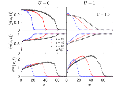
Figure 3: Position dependence of the average current $\langle j(x,t)\rangle$, occupation $\langle n(x,t)\rangle$, and operator entanglement entropy $S^{\text{op}}(x,t)$ for various times, indicating a balistic propagation of the front, irrespective of the interaction strength. For $U=0$, the average current $\langle j(x,t)\rangle$ and occupation $\langle n(x,t)\rangle$, obtained with the $3^{rd}QT$ are displayed with solid lines. Bond dimension were fixed to $M=500$, and the system size is $N=100$.

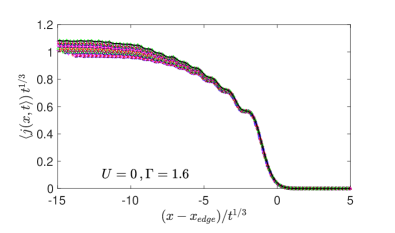
Figure 4: Scaling collapse of the current profile near the edge of the front, $x_{\text{edge}}$, for different times showing a staircase structure in the non-interacting limit $U=0$. Here we display the scaling of the front for 20 different times between $t_{1}=25$ and $t_{2}=35$ equally spaced at an interval $\Delta t=0.5$.

First we focus on the position dependent occupation, $n(x)$, and the current $j(x)$ between neighboring sites $x$ and $x+1$, defined as

$$n(x) \equiv\sum_{\sigma}c^{\dagger}_{x\sigma}c_{x\sigma}\,,$$ (29)

$$j(x) \equiv-i\sum_{\sigma}(c^{\dagger}_{x\sigma}c_{x+1\sigma}-c^{\dagger}_{x+1\sigma}c_{x\sigma}).$$ (30)

The profiles of $\langle j(x,t)\rangle$ and $\langle n(x,t)\rangle$ are displayed in Fig. 3 at different times. The data show a qualitative difference between the non-interacting and interacting cases.

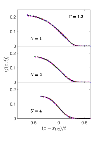
Figure 5: Scaling collapse of the average current profiles $\langle j(x,t)\rangle$ indicating ballistic propagation and a linear in time broadening of the front for any finite $U$ near the $x_{1/2}$ front edge. In each panel we display the scaling of the front for 20 random times between $t_{1}=10$ and $t_{2}=35$.

In the non-interacting case, $U=0$, the current profile displays a staircase-like structure around the edge of the front, similar to the fronts observed in free fermion systems, evolved from a state with a density step-like initial condition Eisler and Rácz (2013). As obvious from the first panel on the left in Fig. 3, the front spreads ballistically with a velocity $v_{0}=J=1$, i.e., the maximal velocity of free quasiparticles. At the same time, we observe a $\sim t^{1/3}$ broadening of the front, characteristic of free Fermions. Eisler and Rácz (2013); Bertini et al. (2016) This is demonstrated in Fig. 4, displaying the appropriately rescaled $\langle j(x,t)\rangle$ curves at the edge of the current profile, $x_{\rm edge}$, where the current starts to have a finite value. As the current profile evolves in time, it assumes a universal shape, and develops a fine staircase-structure, indicative of free, ballistically moving particles.

For finite interactions, $U>0$, a quite different picture emerges. The front still appears to propagate ballistically, with a somewhat reduced velocity, however, the current profile lacks the staircase structure, and the whole profile seems to acquire a universal shape rather than just the front. This hydrodynamics-like time evolution is demonstrated in Fig. 5, where we rescale the front simply by the propagation time, $t$, around the position $x_{1/2}$, where the average current is at half maximum, $\langle j(x_{1/2},t)\rangle={1\over 2}\mathrm{max}_{x}(\langle j(x,t)\rangle)$. Notice that the current profile is a function depends on $U$; its height as well as its width is largely suppressed increasing $U$, thus the overall current as well as the front velocity are suppressed with increasing $U$.

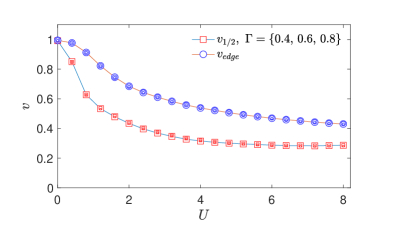
Figure 6: Front velocities $v_{1/2}$ and $v_{\text{edge}}$ as functions of $U$ for different decay rates, $\Gamma$, as extracted from the evolution of the current profile $\langle j(x,t)\rangle$. For each velocity curve, different symbol sizes correspond to different values of $\Gamma$. At $U=0$ we observe $v_{\text{edge}}=1$, the velocity of the fastest non-interacting electrons. Both velocities depend strongly on the interaction $U$ but show no dependence on $\Gamma$.

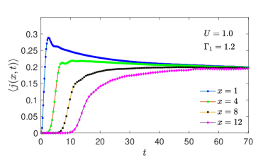
Figure 7: The time dependence of the average current $\langle j(x,t)\rangle$ for various sites along the chain of length $N=100$.

This is quantitatively demonstrated in Fig. 6, where we display the front velocity for different values of $U$ and $\Gamma$. The front velocity can be defined in several ways. It can be defined as the velocity $v_{\text{edge}}$ of the point, $x_{\rm edge}$, where the current raises beyond a pre-defined threshold. One can, however, also define it as the velocity of the point $x_{1/2}$, which we denote as $v_{1/2}$. As shown in Fig. 6, both velocities are reduced by interactions and smaller than the non-interacting velocity. At $U=0$ these two velocities coincide, but for finite $U$ they are clearly different. However, none of them seems to depend on the local disturbance, $\Gamma$. Also, both propagation velocities appear to scale to a finite asymptotic value in the $U\to 0$ limit.

The propagation of the current profile is accompanied by a depletion of particles for $x<x_{\rm edge}$, as demonstrated in the middle panels of Fig. 3. Quite strikingly, the slope of the $\langle n(x,t)\rangle$ curve is reduced with time, but the current remains finite. This clearly shows that, in spite of the interaction, no local equilibrium develops, even far from the front. In local equilibrium, in distinction, the current should be induced by the gradient of the density, $\langle j(x,t)\rangle\propto\partial_{x}\langle n(x,t)\rangle$.

An even more interesting front structure is observed in the entropy. The so-called operator entanglement entropy, $S^{\text{op}}(x,t)$,Prosen and Pižorn (2007) defined as the entanglement entropy of our vectorized state, provides a certain measure of entanglement of the mixed state. The evolution of this quantity is shown in the lower panels of Fig. 3. The operator entanglement spreads also ballistically, however, rather surprisingly, it develops a two-step structure in the interacting case. The first step appears to move with a velocity $v_{\rm edge}$, together with the edge of the current profile. However, the true edge of the entropy profile seems to propagate faster than that, with a velocity, $v_{0}\approx 1$, and penetrates deep into the $\langle n(x,t)\rangle\approx 1$ region, way before the depletion of particles reaches there.

The ballistic spread of the depletion region is natural in the non-interacting case, it is, however quite surprising in the presence of interactions. A ballisticly spreading front implies namely a steady current density, $\lim_{t\to 0}\langle j(x,t)\rangle=j_{\infty}$ for all spatial coordinates $x$, and a corresponding linear increase of the number of lost particles, $N_{\rm out}(t)$, i.e. particles that disappeared in the sink until time $t$. To obtain further confirmation of this ballistic behavior, we computed the current at various positions of the chain as a function of time. This is shown in Fig. 7 for ($U=1$). Within numerical accuracy, the current indeed appears to approach asymptotically a steady state value, independent of the location.

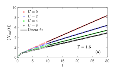
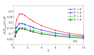
Figure 8: (a) Total particle loss as function of time for different interaction strengths. At large time the total loss rate becomes asymptotically constant, indicating a linear increase of $\langle N_{\rm out}(t)\rangle\sim\gamma\,t$ in time. (b) The total loss rate as function of $\Gamma$ in the quasi stationary regime $t\gg 1/\Gamma$, signaling the presence of the quantum Zeno effect.

The total particle loss $N_{\rm out}(t)$ is shown in Fig. 8(a) as a function of time. It is the largest for $U=0$, and decreases with increasing $U$ such that at any given time $N_{\rm out}^{(U\neq 0)}(t)<N_{\rm tot}^{(U=0)}(t)$. For short times, $t\lesssim 1/\Gamma$, and large enough $\Gamma$, the system is in a transition regime in which particles are lost exponentially at the first site, $N_{\rm out}(t\lesssim 1/\Gamma)\sim(1-e^{-\alpha t/\Gamma})$, where $\alpha$ depends on the initial filling but shows no or very weak dependence on the interaction. At later times, the system reaches a quasi-stationary, non-equilibrium state where the total loss increases linearly in time $N_{\rm out}(t\gg 1/\Gamma)\simeq\gamma\,t$ with a constant loss rate $\gamma=dN_{\rm out}/dt$ that depends on both $U$ and $\Gamma$. The $\Gamma$ dependence is non-monotonic (see the inset in Fig. 8) which can be viewed, similarly to the spinless case Fröml et al. (2019); Wolff et al. (2020), as a manifestation of the quantum Zeno effect Barontini et al. (2013); Fröml et al. (2020) (see Ref. Benenti et al., 2009 for a related effect in a boundary gain/loss driven chain).

V Conclusions

In this work we have developed a non-abelian time evolving block decimation (NA-TEBD) approach to investigate the dynamics of open systems possessing non-Abelian symmetries. By extending the notion of non-Abelian symmetries to the Lindbladian evolution, and organizing the superoperators as symmetry multiplets, we are able to construct an efficient NA-TEBD scheme that explicitly uses abelian as well as non-abelian symmetries of the Lindbladian.

We applied this approach, to the semi-infinite SU(2) Hubbard model with loses at one end of the chain, having an $\textrm{SU(2)}\times\textrm{U(1)}$ symmetry. In the non-interacting limit, $U=0$, we benchmarked our approach against the third quantization approach of Ref. Prosen, 2008, and investigated the time evolution of local density and the current operators as well as the operator entanglement following a dissipation quench in a half-filled, infinite temperature state. In this case particles are depleted around the sink, and a propagating front appears, separating the depleted and occupied regions.

We investigated the structure of the propagating front in detail. Both in the non-interacting and in the interacting limits we find a ballistic front propagation. However, interactions reduce the light cone velocity substantially, $v_{\rm edge}<v_{0}=J=1$. In addition, interactions change, however, drastically the structure of the propagating front. For $U=0$, the front displays coherent fringes, and spreads as $\sim t^{1/3}$,Eisler and Rácz (2013) while for $U\neq 0$ a ballistic $\sim t$ scaling of the whole current profile is observed, and the coherent fringes disappear.

Corroborating these findings and the ballistic front propagation, we observe a saturation of the current to a position independent asymptotic value, $j_{\infty}(U,\Gamma)$, and a corresponding linear increase in the loss of particles, $\textrm{d}N/\textrm{d}t\to j_{\infty}$. The loss rate is suppressed with increasing $U$, however, it exhibits a non-monotonous behavior as a function of the dissipation strength, a clear manifestation of the quantum Zeno effect.

The operator entanglement entropy, $S^{\text{op}}(x,t)$,Prosen and Pižorn (2007) is also found to spread ballistically. However, the true edge of the entropy profile seems to propagate with a velocity, $v_{0}>v_{\rm edge}$, faster than the current profile, and penetrates deep into the $\langle n(x,t)\rangle\approx 1$ region, way before the depletion front reaches there.

The ballistic propagation we observe is somewhat surprising. It implies that the gradient of the density is unrelated to the current density, implying, in turn, the absence of local equilibration. Our simulations are consistent with this picture, while we cannot exclude, however, a slow, e.g. logarithmic suppression of $\textrm{d}N/\textrm{d}t$. It is not clear, either, if the ballistic behavior observed has a relation to the integrability of the Hubbard model.

These results demonstrate the power of this approach. By using explicitly all symmetries of the model, our approach makes it possible to study with high accuracy the dynamics in open systems with relatively large local operator spaces, even on platforms with limited computing power and memory, such as a regular desktop.

Appendix A Third quantization construction

In this section we discuss in more detail the third quantization construction. Following Refs. Prosen (2008); Kos and Prosen (2017) we introduce the Majorana basis, and define the $4N$ operators $w_{m}$ as

$$w_{4x-3}=c_{x\uparrow}+c^{\dagger}_{x\uparrow}\phantom{aaaa}w_{4x-2}=i(c_{x\uparrow}-c^{\dagger}_{x\uparrow})$$

$$w_{4x-1}=c_{x\downarrow}+c^{\dagger}_{x\downarrow}\phantom{aaaa}w_{4x}=i(c_{x\downarrow}-c^{\dagger}_{x\downarrow})\,.$$ (31)

By construction, they satisfy the anticommmutation relations $\{w_{j},w_{k}\}=2\delta_{jk}$. In the Majorana basis the matrix Hamiltonian H corresponding to the hopping term in Eq.  (4) becomes

$$\underline{\underline{H}}={1\over 2}{H}\otimes\sigma_{y}.$$ (32)

The jump operators acting on the first site, are transformed to the Majorana basis as well, and take the general form $F_{1\sigma}\to\sum_{j}l_{\sigma,j}w_{j}$. We can construct the associated Fock space $\cal K$ , i.e. the Liouville space, with dimension $2^{4N}$. A typical orthonormal basis set consists of vectors of the form $|P_{\underline{\alpha}})$, with $P_{\underline{\alpha}}=P_{\alpha_{1}\alpha_{2}\dots\alpha_{4N}}=w_{1}^{\alpha_{1}}w^{\alpha_{2}}\dots w_{4N}^{\alpha_{4N}}$, with $\alpha_{j}\in\{0,1\}$. The annihilation and the creation super-operators can be defined as

$$\hat{c}_{j}|P_{\underline{\alpha}})=\delta_{\alpha_{j},1}|w_{j}P_{\underline{\alpha}})\,\phantom{aaa}\hat{c}^{\dagger}_{j}|P_{\underline{\alpha}})=\delta_{\alpha_{j},0}|w_{j}P_{\underline{\alpha}})$$ (33)

satisfying the cannonical anticommutation relations $\{\hat{c}_{j},\hat{c}^{\dagger}_{j}\}=\delta_{j,k}$. Keeping in mind that the dissipative part of the Lindbladian acts separetly in the even/odd sectors $\cal K=\cal K^{+}\oplus\cal K^{-}$, we can restrict to one of these subspaces. Introducing the dissipative matrix $\underline{\underline{M}}=\underline{\underline{M}}^{r}+i\underline{\underline{M}}^{i}$, where $\underline{\underline{M}}^{r}$ and $\underline{\underline{M}}^{i}$ are the real and imaginary parts of the matrix $M_{ij}=\sum_{\mu}l_{\mu,i}l^{*}_{\mu,j}$. The vectorized Lindblad equation becomes

$$i{d\over dt}|\rho(t))={\hat{L}}\,|\rho(t))$$ (34)

with $-i{\hat{L}}=-2\hat{c}^{\dagger}\underline{\underline{X}}^{T}\hat{c}+4i\hat{c}^{\dagger}{\underline{\underline{M}}}^{i}\hat{c}$. Here $\underline{\underline{X}}^{T}=2i\underline{\underline{H}}+2\underline{\underline{M}}^{r}$. In this way the vectorized Lindblad equation for the density matrix is mapped to a regular Schrödinger equation in the Fock super-operators space. To compute the expectation values and the correlators, one defines the left Liouvillian vacuum, $\langle\mathds{1}|=\langle P_{0,0,\dots 0}|$, in terms of which any two-point correlator (covariance) can be written as $\langle w_{j}w_{k}\rangle=\langle\mathds{1}|\hat{c}_{j}\hat{c}_{k}|\rho\rangle+\delta_{jk}$. The covariance matrix $C_{ij}\equiv\langle w_{i}w_{j}\rangle$ satisfies the associated equation

$${d\over dt}\underline{\underline{C}}(t)=-2\underline{\underline{X}}^{T}\underline{\underline{C}}(t)-2\underline{\underline{C}}(t)\underline{\underline{X}}-8i\underline{\underline{M}}^{i},$$ (35)

which can be solved by standard methods, starting from some initial condition $\underline{\underline{C}}(0)$. Physical observables can be computed from $C_{ij}\equiv\langle w_{i}w_{j}\rangle$. The average occupation number along the Hubbard chain can be obtained, e.g., as

$$\langle n_{j}(t)\rangle=1-{i\over 2}\left(C_{4j-3,4j-2}(t)+C_{4j-1,4j}(t)\right),$$ (36)

and other operators defined on the chain can be constructed in a similar manner.

References

- Harbola and Mukamel (2008) U. Harbola and S. Mukamel, Physics Reports 465, 191 (2008).
- Breuer et al. (2016) H.-P. Breuer, E.-M. Laine, J. Piilo, and B. Vacchini, Rev. Mod. Phys. 88, 021002 (2016).
- Chin et al. (2010) C. Chin, R. Grimm, P. Julienne, and E. Tiesinga, Rev. Mod. Phys. 82, 1225 (2010).
- Müller et al. (2012) M. Müller, S. Diehl, G. Pupillo, and P. Zoller, in Advances in Atomic, Molecular, and Optical Physics, Advances In Atomic, Molecular, and Optical Physics, Vol. 61, edited by P. Berman, E. Arimondo, and C. Lin (Academic Press, 2012) pp. 1 – 80.
- Diehl et al. (2008) S. Diehl, A. Micheli, A. Kantian, B. Kraus, H. P. Büchler, and P. Zoller, Nature Physics 4, 878 (2008).
- Schneider et al. (2012) U. Schneider, L. Hackermüller, J. P. Ronzheimer, S. Will, S. Braun, T. Best, I. Bloch, E. Demler, S. Mandt, D. Rasch, and A. Rosch, Nature Physics 8, 213 (2012).
- Chong et al. (2018) K. O. Chong, J.-R. Kim, J. Kim, S. Yoon, S. Kang, and K. An, Communications Physics 1, 25 (2018).
- Damanet et al. (2019) F. Damanet, E. Mascarenhas, D. Pekker, and A. J. Daley, Phys. Rev. Lett. 123, 180402 (2019).
- Syassen et al. (2008) N. Syassen, D. M. Bauer, M. Lettner, T. Volz, D. Dietze, J. J. García-Ripoll, J. I. Cirac, G. Rempe, and S. Dürr, Science 320, 1329 (2008).
- Cheneau et al. (2012) M. Cheneau, P. Barmettler, D. Poletti, M. Endres, P. Schauß, T. Fukuhara, C. Gross, I. Bloch, C. Kollath, and S. Kuhr, Nature 481, 484 (2012).
- Barontini et al. (2013) G. Barontini, R. Labouvie, F. Stubenrauch, A. Vogler, V. Guarrera, and H. Ott, Phys. Rev. Lett. 110, 035302 (2013).
- Lapp et al. (2019) S. Lapp, J. Ang’ong’a, F. A. An, and B. Gadway, New Journal of Physics 21, 045006 (2019).
- Eckel et al. (2010) J. Eckel, F. Heidrich-Meisner, S. G. Jakobs, M. Thorwart, M. Pletyukhov, and R. Egger, New Journal of Physics 12, 043042 (2010).
- Calabrese et al. (2011) P. Calabrese, F. H. L. Essler, and M. Fagotti, Phys. Rev. Lett. 106, 227203 (2011).
- Buča and Prosen (2012) B. Buča and T. Prosen, New Journal of Physics 14, 073007 (2012).
- Eisert et al. (2015) J. Eisert, M. Friesdorf, and C. Gogolin, Nature Physics 11, 124 (2015).
- Kormos et al. (2017) M. Kormos, M. Collura, G. Takács, and P. Calabrese, Nature Physics 13, 246 (2017).
- Mitra (2018) A. Mitra, Annual Review of Condensed Matter Physics 9, 245 (2018).
- Fukuhara et al. (2013) T. Fukuhara, A. Kantian, M. Endres, M. Cheneau, P. Schauß, S. Hild, D. Bellem, U. Schollwöck, T. Giamarchi, C. Gross, I. Bloch, and S. Kuhr, Nature Physics 9, 235 (2013).
- Lebrat et al. (2019) M. Lebrat, S. Häusler, P. Fabritius, D. Husmann, L. Corman, and T. Esslinger, Phys. Rev. Lett. 123, 193605 (2019).
- Wichterich et al. (2007) H. Wichterich, M. J. Henrich, H.-P. Breuer, J. Gemmer, and M. Michel, Phys. Rev. E 76, 031115 (2007).
- Prosen and Žnidarič (2012) T. Prosen and M. Žnidarič, Phys. Rev. B 86, 125118 (2012).
- Ajisaka et al. (2012a) S. Ajisaka, F. Barra, C. Mejía-Monasterio, and T. Prosen, Phys. Rev. B 86, 125111 (2012a).
- Ajisaka et al. (2012b) S. Ajisaka, F. Barra, C. Mejía-Monasterio, and T. Prosen, Physica Scripta 86, 058501 (2012b).
- Pižorn (2013) I. Pižorn, Phys. Rev. A 88, 043635 (2013).
- Karevski et al. (2013) D. Karevski, V. Popkov, and G. M. Schütz, Phys. Rev. Lett. 110, 047201 (2013).
- Ajisaka et al. (2014) S. Ajisaka, F. Barra, and B. Žunkovič, New Journal of Physics 16, 033028 (2014).
- Arrigoni et al. (2013) E. Arrigoni, M. Knap, and W. von der Linden, Phys. Rev. Lett. 110, 086403 (2013).
- Dorda et al. (2014) A. Dorda, M. Nuss, W. von der Linden, and E. Arrigoni, Phys. Rev. B 89, 165105 (2014).
- Dorda et al. (2015) A. Dorda, M. Ganahl, H. G. Evertz, W. von der Linden, and E. Arrigoni, Phys. Rev. B 92, 125145 (2015).
- Jin et al. (2016) J. Jin, A. Biella, O. Viyuela, L. Mazza, J. Keeling, R. Fazio, and D. Rossini, Phys. Rev. X 6, 031011 (2016).
- Schwarz et al. (2016) F. Schwarz, M. Goldstein, A. Dorda, E. Arrigoni, A. Weichselbaum, and J. von Delft, Phys. Rev. B 94, 155142 (2016).
- Vidal (2003) G. Vidal, Phys. Rev. Lett. 91, 147902 (2003).
- Vidal (2004) G. Vidal, Phys. Rev. Lett. 93, 040502 (2004).
- Verstraete et al. (2004) F. Verstraete, J. J. García-Ripoll, and J. I. Cirac, Phys. Rev. Lett. 93, 207204 (2004).
- Zwolak and Vidal (2004) M. Zwolak and G. Vidal, Phys. Rev. Lett. 93, 207205 (2004).
- Daley et al. (2004) A. J. Daley, C. Kollath, U. Schollwöck, and G. Vidal, Journal of Statistical Mechanics: Theory and Experiment 2004, P04005 (2004).
- White and Feiguin (2004) S. R. White and A. E. Feiguin, Phys. Rev. Lett. 93, 076401 (2004).
- Feiguin and White (2005) A. E. Feiguin and S. R. White, Phys. Rev. B 72, 020404 (2005).
- Haegeman et al. (2013) J. Haegeman, T. J. Osborne, and F. Verstraete, Phys. Rev. B 88, 075133 (2013).
- Zauner-Stauber et al. (2018) V. Zauner-Stauber, L. Vanderstraeten, M. T. Fishman, F. Verstraete, and J. Haegeman, Phys. Rev. B 97, 045145 (2018).
- Vanderstraeten et al. (2019) L. Vanderstraeten, J. Haegeman, and F. Verstraete, SciPost Phys. Lect. Notes , 7 (2019).
- Schollwöck (2005) U. Schollwöck, Rev. Mod. Phys. 77, 259 (2005).
- Werner et al. (2016) A. H. Werner, D. Jaschke, P. Silvi, M. Kliesch, T. Calarco, J. Eisert, and S. Montangero, Phys. Rev. Lett. 116, 237201 (2016).
- Hauschild and Pollmann (2018) J. Hauschild and F. Pollmann, SciPost Phys. Lect. Notes , 5 (2018).
- Jaschke et al. (2018) D. Jaschke, S. Montangero, and L. D. Carr, Quantum Science and Technology 4, 013001 (2018).
- Weichselbaum (2020) A. Weichselbaum, Phys. Rev. Research 2, 023385 (2020).
- Werner et al. (2020) M. A. Werner, C. P. Moca, O. Legeza, and G. Zaránd, Phys. Rev. B 102, 155108 (2020).
- Note (1) This type of symmetry has been defined in Ref. Buča and Prosen (2012) as the weak symmetry, in order to distinguish it from a more restrictive situation of a strong symmetry where and the full set of commute with .
- (50) M. A. Werner, C. P. Moca, O. Legeza, and G. Zaránd, Unpublished .
- Am-Shallem et al. (2015) M. Am-Shallem, A. Levy, I. Schaefer, and R. Kosloff, “Three approaches for representing lindblad dynamics by a matrix-vector notation,” (2015), arXiv:1510.08634 [quant-ph] .
- Krapivsky et al. (2019) P. L. Krapivsky, K. Mallick, and D. Sels, Journal of Statistical Mechanics: Theory and Experiment 2019, 113108 (2019).
- Sels and Demler (2020) D. Sels and E. Demler, Annals of Physics 412, 168021 (2020).
- Fröml et al. (2019) H. Fröml, A. Chiocchetta, C. Kollath, and S. Diehl, Phys. Rev. Lett. 122, 040402 (2019).
- Fröml et al. (2020) H. Fröml, C. Muckel, C. Kollath, A. Chiocchetta, and S. Diehl, Phys. Rev. B 101, 144301 (2020).
- Wolff et al. (2020) S. Wolff, A. Sheikhan, S. Diehl, and C. Kollath, Phys. Rev. B 101, 075139 (2020).
- Kepesidis and Hartmann (2012) K. V. Kepesidis and M. J. Hartmann, Phys. Rev. A 85, 063620 (2012).
- Labouvie et al. (2016) R. Labouvie, B. Santra, S. Heun, and H. Ott, Phys. Rev. Lett. 116, 235302 (2016).
- Jaksch (2008) D. Jaksch, Nature Physics 4, 906 (2008).
- Lieb and Wu (1968) E. H. Lieb and F. Y. Wu, Phys. Rev. Lett. 20, 1445 (1968).
- Ogata and Shiba (1990) M. Ogata and H. Shiba, Phys. Rev. B 41, 2326 (1990).
- Essler et al. (2005) F. H. Essler, H. Frahm, F. Göhmann, A. Klümper, and V. E. Korepin, The one-dimensional Hubbard model (Cambridge University Press, 2005).
- Lindblad (1976) G. Lindblad, Communications in Mathematical Physics 48, 119 (1976).
- Breuer and Petruccione (2002) H.-P. Breuer and F. Petruccione, The Theory of Open Quantum Systems (Oxford University Press, 2002).
- Manzano (2020) D. Manzano, AIP Advances 10, 025106 (2020).
- Bolaños and Barberis-Blostein (2015) M. Bolaños and P. Barberis-Blostein, Journal of Physics A: Mathematical and Theoretical 48, 445301 (2015).
- Dzhioev and Kosov (2011a) A. A. Dzhioev and D. S. Kosov, The Journal of Chemical Physics 134, 044121 (2011a).
- Jiang et al. (2013) M. Jiang, S. Luo, and S. Fu, Phys. Rev. A 87, 022310 (2013).
- Note (2) Notice that, to differentiate between a state that belongs to or we use slightly different ket-bra notations.
- Note (3) Within the time evolution we set .
- Ashida et al. (2020) Y. Ashida, Z. Gong, and M. Ueda, “Non-hermitian physics,” (2020), arXiv:2006.01837 [cond-mat.mes-hall] .
- Dzhioev and Kosov (2011b) A. A. Dzhioev and D. S. Kosov, The Journal of Chemical Physics 135, 174111 (2011b).
- Dzhioev and Kosov (2012) A. A. Dzhioev and D. S. Kosov, Journal of Physics: Condensed Matter 24, 225304 (2012).
- Braun et al. (2013) S. Braun, J. P. Ronzheimer, M. Schreiber, S. Hodgman, T. Rom, I. Bloch, and U. Schneider, Science (New York, N.Y.) 339, 52 (2013).
- Tarruell and Sanchez-Palencia (2018) L. Tarruell and L. Sanchez-Palencia, Comptes Rendus Physique 19, 365 (2018), quantum simulation / Simulation quantique.
- Prosen (2008) T. Prosen, New Journal of Physics 10, 043026 (2008).
- Kos and Prosen (2017) P. Kos and T. Prosen, Journal of Statistical Mechanics: Theory and Experiment 2017, 123103 (2017).
- Eisler and Rácz (2013) V. Eisler and Z. Rácz, Phys. Rev. Lett. 110, 060602 (2013).
- Bertini et al. (2016) B. Bertini, M. Collura, J. De Nardis, and M. Fagotti, Phys. Rev. Lett. 117, 207201 (2016).
- Prosen and Pižorn (2007) T. Prosen and I. Pižorn, Phys. Rev. A 76, 032316 (2007).
- Benenti et al. (2009) G. Benenti, G. Casati, T. Prosen, D. Rossini, and M. Žnidarič, Phys. Rev. B 80, 035110 (2009).
- Note (4) Any operator in the Majorana basis is denoted as A, while in the original basis it is denoted as .