Bayesian Optimization of Function Networks

Abstract

We consider Bayesian optimization of the output of a network of functions, where each function takes as input the output of its parent nodes, and where the network takes significant time to evaluate. Such problems arise, for example, in reinforcement learning, engineering design, and manufacturing. While the standard Bayesian optimization approach observes only the final output, our approach delivers greater query efficiency by leveraging information that the former ignores: intermediate output within the network. This is achieved by modeling the nodes of the network using Gaussian processes and choosing the points to evaluate using, as our acquisition function, the expected improvement computed with respect to the implied posterior on the objective. Although the non-Gaussian nature of this posterior prevents computing our acquisition function in closed form, we show that it can be efficiently maximized via sample average approximation. In addition, we prove that our method is asymptotically consistent, meaning that it finds a globally optimal solution as the number of evaluations grows to infinity, thus generalizing previously known convergence results for the expected improvement. Notably, this holds even though our method might not evaluate the domain densely, instead leveraging problem structure to leave regions unexplored. Finally, we show that our approach dramatically outperforms standard Bayesian optimization methods in several synthetic and real-world problems.

1 Introduction

We consider Bayesian optimization (BO) of objective functions defined by a series of time-consuming-to-evaluate functions, $f_{1},\ldots,f_{K}$, arranged in a directed acyclic network, so that each function takes as input the output of its parent nodes. As we detail below, these problems arise in BO-based policy search in reinforcement learning (Lizotte et al.,, 2007), optimization of complex systems modeled via simulation, and calibration of time-consuming physics-based models.

To illustrate, we introduce a running example of vaccine manufacturing (Sekhon and Saluja,, 2011), focusing on the portion of the manufacturing process that uses live cells to produce proteins needed in a vaccine. It begins with a cell culture, in which living cells are grown and used as “factories” to produce proteins. This process is controlled by a vector, $x_{1}$, containing the temperature, pH, and CO₂ content used when growing these cells. The output of this process is the quantity of the desired protein $y_{1}=f_{1}(x_{1})$, i.e., the yield of this step, along with other byproducts. This output is passed into a second process, purification, which removes byproducts and is controlled by a vector $x_{2}$ comprising temperature, pressure, and flow rate. The yield of the desired protein from this second step is $y_{2}=f_{2}(x_{2},y_{1})$. This output enters a third step, formulation, in which we formulate the raw protein into a form that can be distributed as controlled by a third set of parameters. This determines the yield of the overall process $y_{3}=f_{3}(x_{3},y_{2})$. We wish to choose $(x_{1},x_{2},x_{3})$ to maximize overall protein yield. This problem is summarized as a function network in Figure 1.

The problem described above and other similar problems can be tackled with Bayesian optimization (BO), which has been shown to perform well compared to other derivative-free global optimization methods for time-consuming-to-evaluate objective functions (Snoek et al.,, 2012; Frazier,, 2018). A standard BO algorithm would fit a Gaussian process (GP) (Rasmussen and Williams,, 2006) model on the objective function ($y_{3}$, which depends on $(x_{1},x_{2},x_{3})$) and use it, along with an acquisition function, to sequentially choose the points to evaluate. Under this standard approach, however, evaluations of the intermediate nodes, $f_{1},\ldots,f_{K-1}$, would be ignored despite being available when computing the objective function. In the example above, this corresponds to looking only at the yield of the overall process, and not of each individual step.

Figure 1: Vaccine manufacturing as a function network. Protein $y_{1}=f_{1}(x_{1})$ is created, then purified with yield $y_{2}=f_{2}(x_{2},y_{1})$, and formulated with yield $y_{3}=f_{3}(x_{3},y_{2})$. The goal is to find $(x_{1},x_{2},x_{3})$ that maximizes $y_{3}$.

In this paper, we introduce a novel BO approach that leverages function network structure for substantially more efficient optimization. This approach models the individual nodes of the network using distinct GPs. This allows incorporating observations of each node’s output recursively into a non-Gaussian posterior on the network’s overall output. Our approach then chooses the points to evaluate using the expected improvement (Jones et al.,, 1998) computed with respect to this implied posterior on the objective function. The non-Gaussian nature of this posterior prevents the expected improvement from having a closed form. However, we show that it can still be efficiently maximized via sample average approximation (Kleywegt et al.,, 2002).

Our approach can outperform standard BO by leveraging information from internal nodes unavailable to standard methods. We briefly explain one way this can happen, in the context of the example above. In vaccine manufacturing, each function $f_{k}(x_{k},y_{k-1}),\ k=2,3$, is bounded between $0$ and $y_{k-1}$ because new protein cannot be created in the purification and formulation stages. Moreover, application experts have a prior on what values for $f_{k}(x_{k},y_{k-1})/y_{k-1}$ should be achievable if $x_{k}$ is set well. Thus, if we see that $y_{3}$ is unexpectedly poor, information from intermediate nodes can be extremely valuable: if $y_{1}$ and $y_{2}$ are as expected, then this suggests the problem is with $x_{3}$; if $y_{1}$ is as expected but $y_{2}$ is poor, then the problem is likely with $x_{2}$; and if $y_{1}$ is poor then the problem is likely with $x_{1}$. (If there is a problem with $x_{k}$, there may also be a problem with $x_{k^{\prime}}$, $k^{\prime}>k$, but we can focus on fixing $x_{k}$ first.) Thus, by observing intermediate nodes, we can instantly reduce the effective dimensionality of the input space by a factor of $K=3$.

We show that our method is asymptotically consistent, i.e., that it discovers the global optimum given sufficiently many samples. Remarkably, in contrast with most BO methods, it may do so without measuring densely over the feasible domain, instead leveraging function network structure to exclude regions as unnecessary to explore. This indicates the power of function network structure to improve query efficiency.

We demonstrate through numerical experiments that access to additional information available in a problem formulated as a function network can dramatically accelerate optimization. We study four synthetic problems and four real-world problems: a manufacturing problem similar in spirit to the vaccine example above, an active learning problem with a robotic arm, and two problems arising in epidemiology, one calibrating an epidemic model and the other designing a testing strategy to control the spread of COVID-19. Our method significantly outperforms competing methods that utilize less information, in some cases by $\sim$5% and in other cases by several orders of magnitude.

2 Related Work

Our work occurs within BO, a framework for global optimization of expensive-to-evaluate black-box functions that originated with the work of Zhilinskas, (1975) and Močkus, (1975), and has recently become popular due to its remarkable performance in hyperparameter tuning of machine learning algorithms (Snoek et al.,, 2012; Swersky et al.,, 2013; Wu et al.,, 2019). We refer the reader to Shahriari et al., (2016) and Frazier, (2018) for modern introductions to BO.

Our approach can be catalogued as a grey-box BO method since it does not treat the objective function entirely as a black box, and instead exploits known structure to improve sampling efficiency. Other examples of grey-box BO approaches include multi-fidelity BO (Kandasamy et al.,, 2017; Wu et al.,, 2019), which leverages cheaper approximations of the objective function; BO of objective functions that are the integral of an expensive-to-evaluate integrand (Williams et al.,, 2000; Toscano-Palmerin and Frazier,, 2018; Cakmak et al.,, 2020); BO of objective functions that are a sum of squared errors (Uhrenholt and Jensen,, 2019); and, more generally, BO of objective functions that are the composition of an expensive-to-evaluate inner function and a known inexpensive-to-evaluate outer function (Astudillo and Frazier,, 2019), of which our work can be seen as a significant generalization. We refer the reader to Astudillo and Frazier, (2021) for a tutorial on grey-box BO.

Our work is also closely related to Marque-Pucheu et al., (2019), which proposes a method for efficient sequential experimental design of nested computer codes, also using GPs. This work focuses on the case where there are only two node functions, and one takes as input the output of the other. In contrast with our work, the goal of the proposed method is to learn the output code as accurately as possible within a limited evaluation budget, but optimization is not pursued.

Optimization of composite (a.k.a nested) functions has also been considered in the gradient-based optimization literature (Shapiro,, 2003; Drusvyatskiy and Paquette,, 2019; Charisopoulos et al.,, 2021; Balasubramanian et al.,, 2020). In contrast with ours, these works assume that evaluations are inexpensive, and often also some form of convexity, along with availability of gradients. However, this literature is similar in spirit to ours in that information from inner functions improves efficiency.

Function networks arise in many application areas. While these applications have not, to our knowledge, been previously formulated as specific instances of the general function network model we propose, their literatures are nonetheless relevant to our work.

• In engineering and aerospace design, function networks arise in multidisciplinary optimization (Cramer et al.,, 1994; Amaral et al.,, 2014; Benaouali and Kachel,, 2019), where simulators focusing on different physical laws are coupled into a function network. For example, a simulation of airflow over a wing may output the forces on the wing to another simulation of mechanical stress on the wing structure.

• In drug discovery and materials design, function networks arise from the sequence-structure-function (Sadowski and Jones,, 2009) and composition-structure-property (Hattrick-Simpers et al.,, 2016) paradigms. Here, decision variables (composition, e.g., what fraction of what raw materials are used) determine the structure of the material (how the atoms combine together), which in turn determines how the material behaves (properties).

• Function networks arise in the design of queuing networks (Fu and Henderson,, 2017; Arcelli,, 2020). This includes manufacturing systems (Ghasemi et al.,, 2018), where the partially-processed output of one workstation is input to the next workstation, the design of service systems (Wang et al.,, 2020) such as hospitals and airport security checkpoints, and choosing traffic signal timings for a city’s street network (Osorio and Bierlaire,, 2013).

• Finally, function networks arise in reinforcement learning (Sutton and Barto,, 2018) and Markov decision processes (Puterman,, 1990), where the transition kernel transforms the state variable at the start of a time range to another state variable at the end of this range. This outputted state variable is the input to the next time range. §5.2 shows an example.

3 Problem Setting

We consider objective functions evaluated via a series of functions, $f_{1},\ldots,f_{K}$, arranged in a directed network so that each function in this network takes as input the output of its parent nodes, and assume that evaluating this collection of functions is time-consuming. The network structure is encoded as a directed graph with nodes $V=\{1,\ldots,K$} and directed edges $E=\{(j,k):f_{k}\textnormal{ take as input the output of }f_{j}\}$. We assume that this graph is acyclic and has a single leaf node whose output is the objective to optimize.

Let $J(k)$ denote the set of parent nodes of node $k$. We assume, without loss of generality, that the nodes are ordered such that $j<k$ for all $j\in J(k)$. In addition to the output of its parent nodes, we assume that each function, $f_{k}$, takes as input a (potentially empty) subset, $I(k)\subset\{1,\ldots,D\}$, of the components of the decision vector $x\in\mathbb{R}^{D}$.

Let $h_{1}(x),\ldots,h_{K}(x)$ denote the values of the $K$ nodes in the function network when it is evaluated at $x$. These values are defined recursively by

$$h_{k}(x)=f_{k}\left(x_{I(k)},h_{J(k)}(x)\right),\ k=1,\ldots,K,$$

i.e., by evaluating each function in the network as the values of its parent nodes become available. This recursion is well-defined by our assumption that the graph is acyclic. The objective function is then $g=h_{K}$, and the goal is to solve

$$\max_{x\in\mathbb{X}}g(x),$$

where $\mathbb{X}\subset\mathbb{R}^{D}$ is a simple compact set, such as a hyper-rectangle.

The standard BO approach to this problem models $g$ using a GP prior distribution. This approach iteratively chooses the next point at which to evaluate $g$ as follows. Given $n$ observations of the objective function, $g(x_{1}),\ldots,g(x_{n})$, it computes the posterior distribution on $g$, which is itself a GP. It then uses this posterior distribution to compute an acquisition function (Frazier,, 2018) that quantifies the value of the information that would result from a function evaluation at any given point. Finally, it chooses the next point to evaluate, $x_{n+1}$, as the point that maximizes this acquisition function. Notably, although the outputs of $f_{1},\ldots,f_{K-1}$ would be observed as part of this approach, these evaluations would be ignored by standard BO when calculating the posterior distribution and corresponding acquisition function.

4 Bayesian Optimization with Full Network Observations

This section describes our approach. Like standard BO, it consists of a statistical model and an acquisition function. Unlike standard BO, however, our approach leverages the network structure of the problem by utilizing intermediate outputs within the network. As we describe below, this is achieved by modeling the node functions, $f_{1},\ldots,f_{K}$, as GPs, which in turn implies a non-Gaussian distribution on $g$ (§4.1). Our acquisition function is the expected improvement under this posterior distribution (§4.2), which no longer has a closed form and thus we maximize it via sample average approximation (§4.3). We end up this section by proving that our acquisition function is asymptotically consistent despite not necessarily sampling $\mathbb{X}$ densely (§4.4).

4.1 Statistical Model

Instead of modeling $g$ directly, we model $f_{1},\ldots,f_{K}$, as drawn from independent GP prior distributions. Let $\mu_{0,k}$ and $\Sigma_{0,k}$ denote the prior mean and covariance functions of $f_{k},\ k=1,\ldots,K$, respectively. When $g$ is evaluated at $x$, we also get to observe the value of $f_{k}$ at $\left(x_{I(k)},h_{J(k)}(x)\right)$. Thus, after querying $g$ at $n$ points, $x_{\ell},\ \ell=1,\ldots,n$, the observations of the values of $f_{k},\ k=1,\ldots,K,$ at $\left(x_{\ell,I(k)},h_{J(k)}\left(x_{\ell}\right)\right)$, $\ell=1,\ldots,n$, imply posterior distributions on $f_{1},\ldots,f_{K}$, which are again (conditionally) independent GPs with mean and covariance functions $\mu_{n,k}$ and $\Sigma_{n,k}$, $k=1,\ldots,K$. These can be computed in closed form using the standard GP regression equations (see, e.g., Rasmussen and Williams, 2006). For completeness, we include these equations in §F of the supplement.

The posterior distributions on $f_{1},\ldots,f_{K}$, described above imply a posterior distribution on $g$. This distribution is in general non-Gaussian. Thus, unlike in the standard setting, where $g$ is modeled as a GP, classical acquisition functions such as the expected improvement cannot be computed in closed form. However, as we describe next, drawing samples from this distribution is simple.

Thanks to the acyclic structure of the underlying network that defines $g$, a sample, $\widehat{g}(x)=\widehat{h}_{K}(x)$ from the posterior distribution on $g$ at $x$ can be obtained following the iterative process described next. In each iteration, $k=1,\ldots,K$, we obtain a sample, $\widehat{h}_{k}(x)$, from the posterior distribution on $h_{k}(x)$ by drawing a sample from the normal distribution with mean $\mu_{n,k}\left(x_{I(k)},\widehat{h}_{J(k)}(x)\right)$ and standard deviation

$$\sigma_{n,k}\left(x_{I(k)},\widehat{h}_{J(k)}\right)=\Sigma_{n,k}\left(x_{I(k)},\widehat{h}_{J(k)}(x),x_{I(k)},\widehat{h}_{J(k)}(x)\right)^{1/2}.$$

Supporting efficient calculation, the samples $\widehat{h}_{J(k)}(x)$ will have already been obtained in previous iterations of the for loop since $j<k$ for all $j\in J(k)$ (Note that $J(1)=\emptyset$). This procedure is summarized in Algorithm 1.

0:  $x\in\mathbb{X}$

1:  for $k=1,\ldots,K$ do

2:      $\widehat{h}_{k}(x)\sim\mathcal{N}\left(\mu_{n,k}\left(x_{I(k)},\widehat{h}_{J(k)}(x)\right),\sigma_{n,k}\left(x_{I(k)},\widehat{h}_{J(k)}(x)\right)^{2}\right)$

3:  end for

4:  return  $\widehat{g}(x)=\widehat{h}_{K}(x)$

Algorithm 1 Draw one sample from the posterior on $g(x)$

We end this section by noting that, while the statistical model described above could be catalogued as a deep GP (Damianou and Lawrence,, 2013), in the sense that we have GP layers in an architecture described by a directed acyclic graph, inference in our model is faster. Typically, deep GP inference requires marginalization over latent values of GP layers. In our setting, however, observation structure creates conditional independence across layers, avoiding the need to marginalize.

4.2 Expected Improvement for Function Networks

Our acquisition function is the expected improvement, computed with respect to the implied posterior distribution on $g$ under the statistical model described in §4.1:

$$\textnormal{EI-FN}_{n}(x)=\mathbb{E}_{n}\left[\{g(x)-g_{n}^{*}\}^{+}\right],$$

where $g_{n}^{*}=\max_{i=1,\ldots,n}g\left(x_{n}\right)$ is the best value observed so far, and $\mathbb{E}_{n}$ is the expectation computed with respect to the GP time-$n$ posterior distributions on $f_{1},\ldots,f_{K}$. To distinguish it from the classical expected improvement, we refer to our acquisition function as the expected improvement for function networks (EI-FN) in the remainder of this work.

4.3 Maximization of EI-FN via Sample Average Approximation

Since the posterior distribution on $g$ is non-Gaussian, in contrast with the classical expected improvement acquisition function, $\textnormal{EI-FN}_{n}$ does not admit a closed form expression. However, $\textnormal{EI-FN}_{n}(x)$ can be computed with arbitrary precision following a simple Monte Carlo (MC) approach:

$$\textnormal{EI-FN}_{n}(x)\approx\frac{1}{M}\sum_{m=1}^{M}\left\{\widehat{g}(x)^{(m)}-g_{n}^{*}\right\}^{+},$$

where $\widehat{g}(x)^{(1)},\ldots,\widehat{g}(x)^{(M)}$ are samples drawn from the posterior distribution on $g(x)$, which can be obtained following the approach described in §4.1.

Following the above MC scheme to approximately compute EI-FN, one can aim to maximize this function using a derivative-free global optimization algorithm for inexpensive-to-evaluate functions, such as CMA (Hansen,, 2016), by drawing samples, $\widehat{g}(x)^{(1)},\ldots,\widehat{g}(x)^{(M)}$ independently for each $x$ at which $\textnormal{EI-FN}_{n}$ is evaluated. However, this approach is slow since evaluations of EI-FN are noisy and derivative information is not leveraged. Instead, we propose to maximize EI-FN following a sample average approximation (SAA) approach (Kleywegt et al.,, 2002; Balandat et al.,, 2020).

Succinctly, the SAA approach works by building a MC approximation of EI-FN that is deterministic given a finite set of random variables not depending on $x$, and maximizing this approximation instead of EI-FN itself. The key observation for creating this approximation is that a sample, $\widehat{g}(x)$, can be obtained as $\widehat{g}(x)=\widehat{h}_{K}(x)$, where $\widehat{h}_{1}(x),\ldots,\widehat{h}_{K}(x)$ are defined recursively by

$$\widehat{h}_{k}\left(x;Z\right)={} \mu_{n,k}\left(x_{I(k)},\widehat{h}_{J(k)}(x;Z)\right)+\sigma_{n,k}\left(x_{I(k)},\widehat{h}_{J(k)}(x;Z)\right)Z_{k},$$

where $Z=\left(Z_{1},\ldots,Z_{K}\right)^{\top}$ is a standard normal random vector, and we write $\widehat{h}_{k}(x)$ as $\widehat{h}_{k}\left(x;Z\right)$ to make its dependence on $Z$ explicit. Analogously, we also write $\widehat{g}(x)$ as $\widehat{g}(x;Z)$. This can be seen as an extension of the so-called reparametrization trick for acquisition functions (Wilson et al.,, 2018).

If we now fix $M$ samples drawn from the $K$-dimensional standard normal distribution, $Z^{(1)},\ldots,Z^{(M)}$, then

$$\widehat{\textnormal{EI-FN}}_{n}\left(x;Z^{(1:M)}\right):=\frac{1}{M}\sum_{m=1}^{M}\left\{\widehat{g}\left(x;Z^{(m)}\right)-g_{n}^{*}\right\}^{+}$$

is a MC approximation of EI-FN that is deterministic given $Z^{(1)},\ldots,Z^{(M)}$, as desired. Moreover, Proposition A.0 below shows that, under mild regularity conditions, any maximizer of the above SAA converges in probability exponentially fast to a maximizer of $\textnormal{EI-FN}_{n}$ as $M\rightarrow\infty$, thus suggesting that in practice it is safe to use small values of $M$. This result is a generalization of Theorem 1 in Balandat et al., (2020). Its proof can be found in §A of the supplement.

Proposition 1.

Suppose that the functions $\mu_{n,k}$ and $\sigma_{n,k}$, $k=1,\ldots,K$, are all Lipschitz continuous and let

$$\widehat{x}_{*}^{(M)}\in\operatorname*{argmax}_{x\in\mathbb{X}}\widehat{\textnormal{EI-FN}}_{n}\left(x;Z^{(1:M)}\right),\quad X_{*}=\operatorname*{argmax}_{x\in\mathbb{X}}\textnormal{EI-FN}_{n}(x).$$

Then, for every $\epsilon>0$, there exist $A,\alpha>0$ such that $\mathbb{P}\left(\textnormal{dist}\left(\widehat{x}_{*}^{(M)},X_{*}\right)>\epsilon\right)\leq Ae^{-\alpha M},\ M\in\mathbb{N}$.

Finally, we note that $\widehat{\textnormal{EI-FN}}_{n}$ is differentiable with respect to $x$, provided that $\mu_{k,n}$ and $\Sigma_{k,n}$, $k=1,\ldots,K$, are all differentiable. Thus, $\widehat{\textnormal{EI-FN}}_{n}$ can be maximized using a gradient-based deterministic optimization algorithm such as L-BFGS-B (Byrd et al.,, 1995), with multiple restarts.

4.4 Asymptotic Consistency of EI-FN without Dense Measurements

To shed light on the convergence properties of the expected improvement acquisition function under our statistical model, we prove that, under suitable regularity conditions, EI-FN is asymptotically consistent, meaning that it finds the global optimum of the objective function as the number of evaluations grows to infinity. This builds on results shown for the classical expected improvement (Vazquez and Bect,, 2010; Bect et al.,, 2019) and the expected improvement for composite functions (Astudillo and Frazier,, 2019), and we rely on similar assumptions. This result is stated in Theorem 1 below and its proof can be found in §B of the supplement.

Theorem 1.

Suppose that $x_{n+1}\in\operatorname*{argmax}_{x\in\mathbb{X}}\textnormal{EI-FN}_{n}(x)$ for all $n$. Then, under regularity conditions stated precisely in the supplement, $g_{n}^{*}\rightarrow\max_{x\in\mathbb{X}}g(x)$ as $n\rightarrow\infty$ almost surely under the prior distribution on $f_{1},\ldots,f_{K}$.

Significant novelty in our proof arises from the fact that EI-FN’s measurements are not necessarily dense in $\mathbb{X}$. In nearly all existing work, consistency of BO methods is shown by first showing that the measurements are dense in the objective’s domain (see, e.g., Vazquez and Bect, 2010). Surprisingly, the function network structure may allows us to exclude certain regions of $\mathbb{X}$ as suboptimal after only finitely many measurements, allowing our method to be consistent without measuring everywhere. Such ability gives insight into EI-FN’s strong empirical performance compared to methods ignoring function network structure. As stated in Proposition 2 below, we provide a function network where EI-FN provides a consistent estimate of the global optimum without sampling densely.

Proposition 2.

There exists a function network (detailed in §C of the supplement) in which EI-FN is consistent but whose measurements are not necessarily dense in $\mathbb{X}$.

5 Numerical Experiments

We compare the performance of our algorithm (EI-FN) against the classical expected improvement (EI), i.e., the expected improvement under a GP model over $g$. We also compare with the performance of two other standard algorithms: the algorithm that chooses the points to evaluate uniformly at random over $\mathbb{X}$ (Random); and the knowledge gradient (KG) (also under a GP model over $g$), a more sophisticated acquisition function that often delivers a better performance than the expected improvement (Wu and Frazier,, 2016). The problems in §5.2 and §5.3 fall within the framework of Astudillo and Frazier, (2019) and we include its proposed EI-CF algorithm as a benchmark. All algorithms were implemented in BoTorch (Balandat et al.,, 2020).

We evaluate on 4 synthetic problems and 5 real-world problems. These are described below or in §D of the supplement, with the supplement describing a manufacturing problem building on §1, a COVID-19 testing problem building on §5.3, and a robot control problem similar to the one described in §5.2. In all problems, a first stage of evaluations is performed using $2(d+1)$ points chosen uniformly at random over $\mathbb{X}$. A second stage (pictured in plots) is then performed using each of the algorithms. Error bars in Figure 2 show the mean of the best objective value observed so far, plus and minus 1.96 times the standard deviation divided by the square root of the number of replications. Since the difference in performance in some of our experiments is better appreciated in a logarithmic scale, we also include plots showing the log₁₀-regret for such experiments in Figure 3. Each experiment was replicated 30 times. Experimental setup details and runtimes are available in the supplement. Code to reproduce our numerical experiments can be found at https://github.com/RaulAstudillo06/BOFN.

5.1 Synthetic Test Functions

We create synthetic test problems by arranging standard test functions from the global optimization literature (Jamil and Yang,, 2013) into function networks. These explore a variety of network structures in an easy-to-reproduce form, and are named after the standard test function used to define the function network. We describe these briefly here and then in full detail in §D of the supplement.

Alpine2 and Rosenbrock both arrange $K$ nodes in series, where each node except the first node takes the output of the previous node as input. Additionally, in Alpine2, each node takes a distinct dimension of the decision vector $x$ as input. In Rosenbrock, $x_{1}$ and $x_{2}$ are inputs to the first node, $x_{2}$ and $x_{3}$ are inputs to the second, and so on. These network architectures arise in manufacturing problems like the example in §1, as well as business operations with queues like boarding an aircraft or fulfilling drive-through orders. For Alpine2 we set $K=6$, and for Rosenbrock we set $K=4.$

Ackley has 3 nodes. The first two nodes each take the same 6-dimensional input. Their outputs are passed to the third node that produces the final output. This type of function network arises in algorithm design for two-sided markets (Li et al.,, 2021), like Uber and AirBnB, where the first node simulates an intervention’s effect on riders (or guests), the second simulates its effect on drivers (or hosts), and the third simulates the matching process where riders and drivers (or guests and hosts) interact to produce transactions.

Drop-Wave has two nodes. The first node takes a two-dimensional vector $x$ as input. This node’s output is passed to the second node, which produces the objective value. This network architecture is representative of multidisciplinary engineering design (Benaouali and Kachel,, 2019), for example in aerospace, where a small number of distinct black-box simulators simulate processes governed by physical laws that affect each other through a small number of channels, such as an aircraft engine simulation (the first node) determining heat generated while flying, which is then inputted to a temperature-dependent simulation of mechanical stress on the aircraft’s frame (the second node).

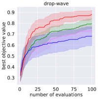
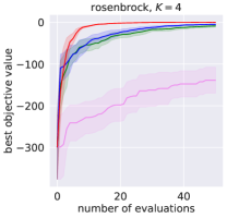
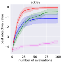
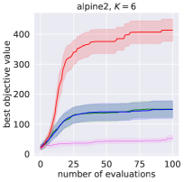
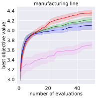
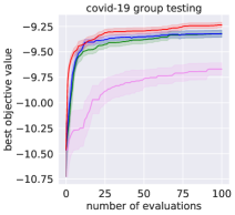
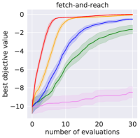
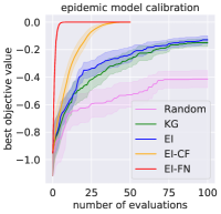
Figure 2: Top: Results on synthetic problems that adapt widely used synthetic test functions into function networks. Bottom: Results on realistic problems: manufacturing line, design of testing protocols for COVID-19, fetch-and-reach with a robotic arm, and calibration of an epidemic model. EI-FN substantially improves over benchmark methods, with larger improvements for problems with higher-dimensional decision vectors and more nodes.

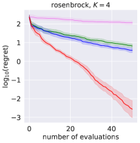
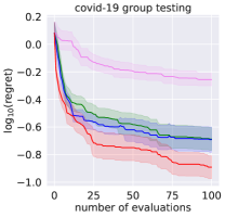
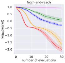
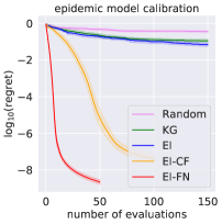
Figure 3: Results on four of our test problems. In contrast with Figure 2 above, which shows the best objective value found, here we plot the log₁₀-regret.

5.2 Fetch-and-Reach with a Robotic Arm

This test problem is obtained by adapting the Fetch environment from OpenAI Gym (see Plappert et al., (2018)). The goal is to move the gripper of a robotic arm to a target location with only three movements. We formulated this problem as a function network with 3 nodes, each representing a movement of the robotic arm. Each of these nodes takes as input the current location of the gripper along with a vector of forces to be applied to the robotic arm in that step, and produces as output the location of the arm after this movement is complete. (Note that the output of each node is 3-dimensional and thus this can also be thought of as a function network with 9 single-output nodes). The objective to minimize is the distance between the gripper and the target in the final step. Figure 4 shows an animation of this problem.

We formalize the above problem as follows. Let $z_{\mathrm{init}},z_{\mathrm{target}}\in\mathbb{R}^{3}$ denote the object’s initial and target locations, respectively. At each time step, $t$, we choose the vector of forces to be applied to the robotic arm $x_{t}\in[-1,1]^{3}$. After this movement, the location of the object becomes $z_{t+1}$. The goal is to choose $x_{t}$ for $t=1,\ldots,T$ to minimize $\|z_{\mathrm{target}}-z_{T}\|_{2}$. We set $z_{\mathrm{init}}=(0,0,0)$, $z_{\mathrm{target}}=(-12,13,0.2)$, and $T=3$. This can be interpreted as a function network by associating each time step with a triplet of node functions $f_{t}=(f_{t,1},f_{t,2},f_{t,3})$ which take $x_{t}$ as input and produce $x_{t+1}=f_{t}(x_{t})$ as output.

A very similar experiment to the one described above can be found in §E of the supplement. It considers a a variation of the active learning for robot pushing problem introduced by Wang and Jegelka, (2017) whose goal is to teach a robot to push an object to a predetermined target location. As in the experiments here, EI-FN outperforms other methods significantly, including EI-CF.

Figure 4: A sequence of screenshots showing three consecutive movements performed by the robotic arm described in §5.2.

5.3 Calibration of an Epidemic Model

Here we consider calibration of compartmental stochastic models to data, a widely-used tool in epidemiology, medical modeling, and ecology (Sandberg,, 1978). Function networks are well-suited to exploit the structure of such models. We focus on calibration of a specific epidemic model for influenza, building toward a COVID-19 mitigation benchmark in the next section. We first describe the epidemic model, then the calibration problem and, finally, formulation as a function network.

SIS Epidemiological Model: We calibrate to data a widely used epidemiological model, the SIS model (see, e.g., Garnett, 2002), that models diseases like influenza capable of reinfecting individuals multiple times. In this model, individuals either do not have the disease and are “susceptible” (S) or have the disease and are “infectious” (I). We consider a SIS model of two interacting populations, where infections occur at population-dependent rates.

The model is dynamic, with time indexed by $t=0,1\ldots,T$. At the beginning of each time period $t$, the fraction of population $i\in\{0,1\}$ that is infectious is $I_{i,t}$. We assume each population is of equal size, $N$. During this time period, each person in group $i$ comes into close physical contact with $\beta_{i,j,t}$ people from group $j$. When this contact is between an infectious person and a susceptible one, it infects the susceptible person. A fraction $I_{j,t}$ of the people from group $j$ involved in such interactions are infectious and a fraction $(1-I_{i,t})$ from group $i$ are susceptible. A number of new infections in group $i$ result, $N(1-I_{i,t})\beta_{i,j,t}I_{j,t}$. As a fraction of group $i$’s population, this is $(1-I_{i,t})\beta_{i,j,t}I_{j,t}$. Summing across $j$, we have $(1-I_{i,t})\sum_{j}\beta_{i,j}(t)I_{j,t}$ new group $i$ infections. At the same time, infections resolve at a rate of $\gamma$ per period. This results in a decrease in the infectious population in group $i$ of $\gamma I_{i,t}$. Putting this together, the number of infectious individuals in group $i$ at the start of the next time period is $I_{i,t+1}=I_{i,t}(1-\gamma)+(1-I_{i,t})\sum_{j}\beta_{i,j,t}I_{j,t}$.

Calibration: The SIS model has parameters $I_{i,0}$, $\gamma$ and $\beta_{i,j,t}$, where $0\leq t<T$ and $i,j\in\{1,2\}$. We calibrate the parameters $\vec{\beta}=(\beta_{i,j,t}:i,j,t)$ while fixing $\gamma=0.5$ and $I_{i,0}=.01$ (for both $i$). We simulate a trajectory of infections from $t=0$ up to $T=3$, using a held-out value for $\vec{\beta}$. We let $I^{\mathrm{obs}}_{i,t}$ denote the fraction of group $i$ observed to be infected at time $t$ in this trajectory. We then search for the vector $\vec{\beta}$ that, when passed to the SIS model, minimizes the mean squared error between this trajectory and the SIS model predictions. Letting $I_{i,t}(\vec{\beta})$ indicate this predicted value, the goal is to minimize the mean-squared error (MSE), $\mathrm{MSE}(\vec{\beta}):=\sum_{t=1}^{T}(I^{\mathrm{obs}}_{i,t}-I_{i,t}(\vec{\beta}))^{2}$. We do not include $t=0$ since $I_{i,0}(\vec{\beta})$ is the same for all $\vec{\beta}$.

Formulation as a Function Network: We encode this as a function network using $2T+1$ nodes, as illustrated in Figure 5. For each time period $t$ and each group $i$, a node takes input $I_{t}:=(I_{j,t}:j=0,1)$ and $\beta_{t}:=(\beta_{j,j^{\prime},t}:j,j^{\prime}\in\{0,1\})$ and produces output $I_{i,t+1}$. (For $t=0$, the input $I_{0}$ is not needed since this is the same for all $\vec{\beta}$.) Then, one additional node takes the output of the other nodes $(I_{i,t}:i=0,1,t=1,\ldots,T)$ as its input and produces the sum of squared errors $\sum_{t=1}^{T}(I^{\mathrm{obs}}_{i,t}-I_{i,t}(\vec{\beta}))^{2}$ as output. We treat this final node as known (its GP prior has a kernel of 0).

EI-CF benchmark: The fact that the final node in this problem (denoted “MSE” in Figure 5) has known structurre permits comparing against the EI-CF method for BO of composite functions (Astudillo and Frazier,, 2019) as a benchmark. EI-CF is substantially less general than our method (EI-FN): it is restricted to settings with one time-consuming black-box multi-output node that provides input to one fast-to-evaluate node with known structure. To apply EI-CF to this problem, the single black-box multi-output node takes $\vec{\beta}$ as input and produces the vector $(I_{i,t}(\vec{\beta}):i,t)$ as output. This output is then supplied to the “MSE” node. This approach ignores the fact that $I_{i,t}$ does not depend on $\beta_{t^{\prime}}$, $t^{\prime}>t$, and depends only indirectly on $\beta_{t^{\prime}}$, $t<t$ through $I_{j,t-1}$, $j=1,2$.

Figure 5: Function network for the (left) epidemic calibration problem in §5.3 and (right) the COVID-19 pooled testing optimization problem described in the supplement.

5.4 Discussion

Across the wide range of problems considered, EI-FN significantly improves query efficiency over standard BO methods that ignore the function network structure of evaluations. The benefits range from a  5% improvement in the value of the best point found on the Drop-Wave and manufacturing problems to several orders of magnitude in the Rosenbrock and epidemic model calibration problems.

The largest benefit arise when the control input is high-dimensional but the input to individual nodes is low-dimensional. On the epidemic model calibration problem, we see EI-CF (Astudillo and Frazier,, 2019) outperforming EI and KG by several orders of magnitude, and EI-FN outperforming EI-CF by several additional orders of magnitude. As noted above, EI-CF can be seen as a special case of EI-FN using a less informative function network that hides observations from some nodes. This is consistent with observations of function network structure allowing substantial improvement in query efficiency, and observing more of the internal function network structure providing more value.

6 Conclusion

We introduced a novel BO approach for objective functions defined by a series of expensive-to-evaluate functions, arranged in a network so that each function takes as input the output of its parent nodes. These objective functions arise in a wide range of application domains. However, existing methods cannot leverage this structure. Our approach models the outputs of the functions in this network instead of only the objective function, as is standard in BO. Our experiments show that, by doing so, this approach can dramatically outperform standard BO methods.

Though we see substantial benefits from our approach, there are limitations. First, it requires more computation than standard BO methods, as explored in the supplement. (When the objective is time-consuming, the improved query efficiency more than makes up for the additional computation required.) Second, while we have demonstrated our method in problems with up to 9 nodes, and computational speed would support more, our method does not (yet) scale to hundreds of nodes. Third, while we show consistency, it would be instructive to complement our empirical results showing fast convergence with a theoretical understanding of convergence rates. Existing approaches to prove convergence rates for the classical expected improvement heavily rely on properties of its analytical expression (Bull,, 2011; Ryzhov,, 2016), and thus are not directly generalizable to our setting. This is, however, an exciting direction for future work.

As with any powerful new method for optimizing time-consuming-to-compute black-box functions, ours can accelerate many applications. While this includes innovations that generally benefit society, such as improvements to public health and vaccine manufacturing, it also includes the design of weapons and other engineering systems that could harm individuals. Thus, it is important that society enact guardrails that ensure proper use of our methodology.

Appendix A Proof of Proposition 1

In this section, we provide a formal statement and proof of Proposition 1. We begin by proving the following auxiliary result.

Lemma A.0.

Suppose that $f:\mathbb{R}^{B_{1}\times\ldots\times B_{J}}\rightarrow\mathbb{R}$ and $h_{j}:\mathbb{R}^{A}\rightarrow\mathbb{R}^{B_{j}},\ j=1,\ldots,J,$ are all Lipischitz continuous with Lipschitz constants $L_{f}$ and $L_{h_{j}},\ j=1,\ldots,J,$ respectively. Then, the function $g:\mathbb{R}^{A}\rightarrow\mathbb{R}$ defined by $g(x)=f(h_{1}(x),\ldots,h_{J}(x))$ is Lipschitz with Lipschitz constant $L_{g}:=L_{f}\sum_{j=1,\ldots,J}L_{h_{j}}$.

Proof.

We have

$$|g(x)-g(x^{\prime})| =|f(h_{1}(x),\ldots,h_{J}(x))-f(h_{1}(x^{\prime}),\ldots,h_{J}(x^{\prime}))|$$

$$\leq L_{f}\|(h_{1}(x),\ldots,h_{J}(x))-(h_{1}(x^{\prime}),\ldots,h_{J}(x^{\prime}))\|_{2}$$

$$\leq L_{f}\sum_{j=1}^{J}\|h_{j}(x)-h_{j}(x^{\prime})\|_{2}$$

$$\leq L_{f}\sum_{j=1}^{J}L_{h_{j}}\|x-x^{\prime}\|_{2}$$

$$=L_{g}\|x-x^{\prime}\|_{2}.$$

∎

We are now in position to show Proposition 1, which can be seen as a simple generalization of Theorem 1 in Balandat et al., (2020).

Proposition A.0 (Proposition 1).

Suppose that $\mathbb{X}$ is compact, and that the functions $\mu_{n,k},\sigma_{n,k}:\mathbb{R}^{|I(k)|}\times\mathbb{R}^{|J(k)|}\rightarrow\mathbb{R}$, $k=1,\ldots,K$, are Lipschitz continuous. Let

$$\widehat{x}_{*}^{(M)}\in\operatorname*{argmax}_{x\in\mathbb{X}}\widehat{\textnormal{EI-FN}}_{n}\left(x;Z^{(1:M)}\right),\quad X_{*}=\operatorname*{argmax}_{x\in\mathbb{X}}\textnormal{EI-FN}_{n}(x),$$

where $\{Z_{m}\}_{m=1}^{\infty}$ are independent standard normal random variables. Then, for every $\epsilon>0$, there exist $A,\alpha>0$ such that $\mathbb{P}\left(\textnormal{dist}\left(\widehat{x}_{*}^{(M)},X_{*}\right)>\epsilon\right)\leq Ae^{-\alpha M}$ for all $M$.

Proof.

Let $L_{\mu_{n,k}}$ and $L_{\sigma_{n,k}}$ be the Lipschitz constants of $\mu_{n,k}$ and $\sigma_{n,k}$, respectively, and consider the functions $\widehat{f}_{n,k}:\mathbb{R}^{|I(k)|}\times\mathbb{R}^{|J(k)|}\times\mathbb{R}\rightarrow\mathbb{R},\ k=1,\ldots,K,$ given by

$$\widehat{f}_{n,k}(x_{I(k)},y_{J(k)},z_{k})=\mu_{n,k}(x_{I(k)},y_{J(k)})+\sigma_{n,k}(x_{I(k)},y_{J(k)})z_{k}.$$

We note that, for any fixed $z_{k}$, the function $(x_{I(k)},y_{J(k)})\mapsto\widehat{f}_{n,k}(x_{I(k)},y_{J(k)},z_{k})$ is $\left(L_{\mu_{n,k}}+L_{\sigma_{n,k}}|z_{k}|\right)$-Lipschitz.

Now consider the functions $\widehat{h}_{n,1},\ldots,\widehat{h}_{n,k}:\mathbb{X}\times\mathbb{R}^{K}\rightarrow\mathbb{R}$ defined recursively by

$$\widehat{h}_{n,k}(x,z)=\widehat{f}_{n,k}\left(x_{I(k)},\widehat{h}_{n,J(k)}(x,z),z_{k}\right),\ k=1,\ldots,K.$$

Applying Lemma 1 repeatedly, we find that, for any fixed $z\in\mathbb{R}^{K}$, the functions $x\mapsto\widehat{h}_{n,k}(x,z),\ k=1,\ldots,K,$ are Lipschitz continuous with Lipschitz constants $L_{\widehat{h}_{n,k}}(z),\ k=1,\ldots,K,$ defined recursively by

$$L_{\widehat{h}_{n,k}}(z)=\left(L_{\mu_{n,k}}+L_{\sigma_{n,k}}|z_{k}|\right)\left(1+\sum_{j\in J(k)}L_{\widehat{h}_{n,j}}(z)\right),\ k=1,\ldots,K.$$

Let $\widehat{g}_{n}=\widehat{h}_{n,k}$ and $L_{\widehat{g}_{n}}=L_{\widehat{h}_{n,k}}$. Then, for any fixed $z$, the function $x\mapsto\widehat{g}_{n}(x,z)$ is $L_{\widehat{g}_{n}}(z)$-Lipschitz. Moreover, by definition, $\widehat{g}_{n}$ satisfies

$$\textnormal{EI-FN}_{n}(x)=\mathbb{E}_{n}\left[\left\{\widehat{g}_{n}(x,Z)-g_{n}^{*}\right\}^{+}\right],$$

where $Z$ is a $K$-dimensional standard normal random vector and also

$$\widehat{\textnormal{EI-FN}}_{n}\left(x;Z^{(1:M)}\right)=\frac{1}{M}\sum_{m=1}^{M}\left\{\widehat{g}_{n}\left(x,Z^{(m)}\right)-g_{n}^{*}\right\}^{+}.$$

Now observe that $L_{\widehat{g}_{n}}(z)$ is a polynomial in the variables $|z_{1}|,\ldots,|z_{k}|$ with degree at most 1 for each variable. Since the folded normal distribution has finite moment generating function everywhere Therefore, if $Z$ is $K$-dimensional standard normal random vector, then $L_{\widehat{g}_{n}}(Z)$ has a finite moment generating function in a neighborhood of 0.

An similar argument can be used to show that, for every $x$, $\widehat{g}_{n}(x,Z)$ has a finite moment generating function in a neighborhood of zero. The desired result is now a direct consequence of Proposition 2 in the supplement of Balandat et al., (2020), which is in turn a consequence of Theorem 2.3 in Homem-de Mello, (2008). ∎

Appendix B Proof of Theorem 1

In this section, we prove Theorem 1. Throughout this section, we let $(x_{n}:n)$ denote the sequence of points at which the function network is evaluated. We begin by introducing the following definition, which is analogous to Definition 2.1 in Bect et al., (2019).

Definition B.1.

Let $\mathcal{F}_{n}$ be the sigma algebra generated by the function network observations up to time $n$. The sequence $(x_{n}:n)$ is said to be a (non-randomized) sequential design if $x_{n}$ is $\mathcal{F}_{n-1}$-measurable for all $n$.

Throughout this section, we assume that $(x_{n}:n)$ is a sequential design. We note, in particular, that if $x_{n}\in\max_{x\in\mathbb{X}}\textnormal{EI-FN}_{n-1}(x)$ for all $n$, then $(x_{n}:n)$ is a sequential design.

Our proof relies on the following assumptions.

Assumption B.1.

$\mathbb{X}$ is compact.

Assumption B.2.

The prior mean and covariance functions of $f_{1},\ldots,f_{K}$, are such that $f_{1},\ldots,f_{K}$ are continuous almost surely.

Assumption B.3.

The prior covariance functions of $f_{1},\ldots,f_{K}$ are bounded.

Assumption B.4.

With probability 1 under the prior, given $f_{1},\ldots,f_{K}$ and a sequential design $(x_{n}:n)$, there exists a function $\beta(z)$ such that $|\widehat{g}_{n-1}(x_{n},z)|\leq\beta(z)$ for all $n$ and $z$ and $\int_{-\infty}^{\infty}\varphi(z)\beta(z)<\infty$, where $\varphi$ is the standard normal pdf.

Assumptions B.1,  B.2, and  B.3 are standard. Assumption B.4 is bespoke to our arguments, but holds, for example, when the posterior mean of $f_{K}$ is uniformly bounded. (This bound can depend on $f_{1},\ldots,f_{K}$.) This occurs, for example, when each $f_{k}$ is in the reproducing kernel Hilbert space (RKHS) corresponding to the prior covariance function. In particular, if $f_{K}$ is in this RKHS and the prior kernel is bounded, then $f_{K}$ is bounded and there is a uniform bound (depending on the RKHS norm of $f_{K}$ and the prior covariance) over the deviation between $f_{K}$ and the sequence of posterior means resulting from our observations. The sum of these two bounds and a term that is linear in $z$ arising from the posterior standard deviation term in the definition of $\widehat{g}_{n-1}(x_{n},z)$ provides $\beta(z)$. We also believe that Assumption B.4 holds more broadly.

Note that our proof does not rely on the no-empty-ball assumption (NEB) of Vazquez and Bect, (2010). Thus, our proof also extends the proof of Astudillo and Frazier, (2019) to a broader class of prior distributions.

As in the main paper, we refer to the “time-$n$” posterior, which is the conditional distribution of $f_{1},\ldots,f_{K}$ given $(x_{m}:m\leq n)$ and $(h_{k}(x_{m}):k\leq K,m\leq n)$. $\mathbb{E}_{n}$ denotes expectation with respect to this conditional distribution, and $\mathbb{P}_{n}$ denotes the probability operator.

Recall the sampling procedure from Section 4.3 of the main paper. This defined a function $\widehat{g}(x,Z)$ that depended on the current posterior distribution, a point $x$ in the feasible domain, and a vector $Z$. When $Z$ was generated as a standard normal random variable, the distribution of $\widehat{g}(x,Z)$ was the same as that of $g(x)$ under the current posterior. To support working with this over a sequence of posterior distributions, we use $\widehat{g}_{n}(x,Z)$ to indicate this function calculated using the posterior at time $n$. We similarly use the notation $\widehat{h}_{k}(x,Z)$ to represent the function $\widehat{h}_{n,k}(x,Z)$ from the main paper computed with respect to the posterior at time $n$.

Lemma B.0.

$g^{*}_{\infty}:=\lim_{n}g^{*}_{n}$ exists and is finite almost surely. Moreover, any limit point $x_{\infty}$ of the sequence $(x_{n}:n)$ satisfies $g(x_{\infty})\leq g^{*}_{\infty}$.

Proof.

The sequence $(g^{*}_{n}:n)$ is non-decreasing and bounded above by the random variable $g^{*}:=\max_{x^{\prime}\in\mathbb{X}}g(x^{\prime})$. The random variable $g^{*}$ is almost surely finite since $g$ is almost surely continuous (it is the composition of a collection of almost surely continuous functions $h_{k}$) and $\mathbb{X}$ is compact. Thus $g^{*}_{\infty}:=\lim_{n}g^{*}_{n}$ exists and is finite almost surely.

Let $x_{\infty}$ be the limit of a convergent subsequence $(x_{n_{m}}:m)$ of $(x_{n}:n)$. Since $g$ is almost surely continuous,

$$g(x_{\infty})=g(\lim_{m}x_{n_{m}})=\lim_{m}g(x_{n_{m}})\leq\lim_{m}g^{*}_{n_{m}+1}\leq\lim_{m}g^{*}_{\infty}=g^{*}_{\infty}.$$

∎

Lemma B.0.

Consider the almost sure event that $f_{k}$ is continuous for all $k=1,\ldots,K$. On this event, the function $h_{k}$ is continuous for all $k=1,\ldots,K$.

Proof.

We show this via induction. The base case, for $k=1$, follows since $f_{1}$ is continuous on the event considered, $x_{I(k)}$ is a continuous function of $x$, and so $h_{1}(x)=f_{1}(x_{I(k)})$ is the composition of two continuous functions and so is a continuous function of $x$.

We now show the induction step. Fix $k>1$. Suppose $h_{k^{\prime}}(x)$ is continuous for all $k^{\prime}<k$. applying the induction hypothesis for all $k^{\prime}\in J(k)\subseteq\{1,\ldots,k-1\}$ implies that $h_{J(k)}(x)$ is continuous. Also $x_{I(k)}$ is a continuous function of $x$. Thus, $x\mapsto(x_{I(k)},h_{J(k)}(x))$ is continuous. This and the fact that $f_{k}$ is continuous on the event considered implies that $h_{k}(x)=f_{k}(x_{I(k)},h_{J(k)}(x))$ is a composition of continuous functions and so is continuous. ∎

Lemma B.0.

For each $k=1,\ldots,K$, the functions $\mu_{n,k}$ and $\sigma_{n,k}$ converge pointwise to some continuous functions $\mu_{\infty,k}$ and $\sigma_{\infty,k}$ almost surely; moreover, this convergence is uniform over compact subsets of $\mathbb{R}^{|I(k)|}\times\mathbb{R}^{|J(k)|}$.

Proof.

Fix $k$ and consider the almost sure event that $f_{1},\ldots,f_{k-1}$ are continuous. Condition on continuous realizations of $f_{1},\ldots,f_{k-1}$, thus fixing $h_{J(k)}$ as well.

Let $A$ be an arbitrary compact subset of $\mathbb{R}^{|I(k)|}\times\mathbb{R}^{|J(k)|}$ and define $B=\{(x_{I(k)},h_{J(k)}(x)):x\in\mathbb{X}\}$. $B$ is compact by Lemma B since $x\mapsto(x_{I(k)},h_{J(k)}(x))$ is continuous, $\mathbb{X}$ is compact, and the image of a compact set through a continuous function is compact. The observations of $f_{k}$ occur at input points $\{(x_{n,I(k)},h_{J(k)}(x_{n})):n\}\subset B$.

Let $C=A\cup B$ and note that $C$ is compact. Then, by Proposition 2.9 in Bect et al., (2019), $\mu_{n,k}$ and $\sigma_{n,k}$ converge uniformly over $C$ and thus also over $A$. ∎

Lemma B.0.

Let $(x_{n_{m}}:m)$ be a convergent subsequence of $(x_{n}:n)$ with limit $x_{\infty}$. Then, $\lim_{m\to\infty}\widehat{g}_{n_{m}-1}(x_{n_{m}},z)=g(x_{\infty})$ for each $z\in\mathbb{R}^{K}$ almost surely.

Proof.

All the convergence claims made in this proof are almost surely. First note that Lemma B implies that, for each $k=1,\ldots,K$, the function $\widehat{f}_{n,k}$ defined in the proof of Proposition 1 converges to the function $\widehat{f}_{\infty,k}$ defined by

$$\widehat{f}_{\infty,k}(x_{I(k)},y_{J(k)},z_{k})=\mu_{\infty,k}(x_{I(k)},y_{J(k)})+\sigma_{\infty,k}(x_{I(k)},y_{J(k)})z_{k}.$$

uniformly in $(x_{I(k)},y_{J(k)})$ (but not necessarily $z_{k}$). This in turn implies that, for each $k=1,\ldots,K$, $\widehat{h}_{n,k}$ converges to the function $\widehat{h}_{\infty,k}$ defined recursively by

$$\widehat{h}_{\infty,k}(x,z)=\widehat{f}_{\infty,k}\left(x_{I(k)},\widehat{h}_{\infty,J(k)}(x,z),z_{k}\right)$$

uniformly in $x\in\mathbb{X}$ for each $z\in\mathbb{R}^{K}$.

We show the following two claims by induction on $k$:

1. $\sigma_{n_{m}-1,k}(x_{n_{m},I(k)},\widehat{h}_{n_{m}-1,J(k)}(x_{n_{m}},z))\to 0$.

2. $\widehat{h}_{n_{m}-1,k}(x_{n_{m}},z)\to h(x_{\infty})$.

We first show the induction step, where we assume the induction hypothesis is true for all $k^{\prime}<k$ and show it for $k$.

Each element of $J(k)$ is strictly less than $k$ and so the induction hypothesis implies that $\widehat{h}_{n_{m}-1,J(k)}(x_{n_{m}},z)\rightarrow h_{J(k)}(x_{\infty})$. Moreover, since $x_{n_{m}}\rightarrow x_{\infty}$, and $\sigma_{n,k}$ converges uniformly to $\sigma_{\infty,k}$, it follows that $\sigma_{n_{m}-1,k}(x_{n_{m},I(k)},\widehat{h}_{n_{m}-1,J(k)}(x_{n_{m}},z))$ converges to $\sigma_{\infty,k}(x_{\infty,I(k)},h_{J(k)}(x_{\infty}))$. Similarly, $\widehat{h}_{n_{m}-1,k}(x_{n_{m}},z)$ converges to

$$\widehat{h}_{\infty,k}(x_{\infty},z) =\widehat{f}_{\infty,k}\left(x_{\infty,I(k)},\widehat{h}_{\infty,J(k)}(x_{\infty},z),z_{k}\right)$$

$$=\widehat{f}_{\infty,k}\left(x_{\infty,I(k)},h_{J(k)}(x_{\infty}),z_{k}\right)$$

$$=\mu_{\infty,k}(x_{\infty,I(k)},h_{J(k)}(x_{\infty}))+\sigma_{\infty,k}(x_{\infty,I(k)},h_{J(k)}(x_{\infty}))z_{k},$$

where the second equation is obtained by noting that, since $\widehat{h}_{n_{m}-1,J(k)}(x_{n_{m}},z)\rightarrow h_{J(k)}(x_{\infty})$ (by the induction hypothesis) and $\widehat{h}_{n_{m}-1,J(k)}(x_{n_{m}},z)\rightarrow\widehat{h}_{\infty,J(k)}(x,z)$, it must be the case that $\widehat{h}_{\infty,J(k)}(x_{\infty},z)=h_{J(k)}(x_{\infty})$.

Now observe that $\sigma_{n_{m}+1,k}(x_{n_{m},I(k)},h_{J(k)}(x_{n_{m}}))$ converges to $\sigma_{\infty,k}(x_{\infty,I(k)},h_{J(k)}(x_{\infty}))$, but $\sigma_{n_{m}+1,k}(x_{n_{m},I(k)},h_{J(k)}(x_{n_{m}}))=0$ for all $m$, and thus $\sigma_{\infty,k}(x_{\infty,I(k)},h_{J(k)}(x_{\infty}))=0$. This proves the first part of the induction step. Similarly, note that $\mu_{n_{m}+1,k}(x_{n_{m},I(k)},h_{J(k)}(x_{n_{m}}))$ converges to $\mu_{\infty,k}(x_{\infty,I(k)},h_{J(k)}(x_{\infty}))$, but

$$\mu_{n_{m}+1,k}(x_{n_{m},I(k)},h_{J(k)}(x_{n_{m}})) =f_{k}(x_{n_{m},I(k)},h_{J(k)}(x_{n_{m}}))$$

$$=h_{k}(x_{n_{m}})\rightarrow h_{k}(x_{\infty}).$$

This proves the second part of the induction step.

The proof of the base case ($k=0$) is analogous except that $J(k)=\emptyset$ eliminates terms that depend on $k^{\prime}<k$.

∎

Lemma B.0.

$\liminf_{n}\textnormal{EI-FN}_{n-1}(x_{n})=0$ almost surely.

Proof.

Since $(x_{n}:n)$ is contained in a compact set, it has a convergent subsequence, $(x_{n_{m}}:m)$.

Then, letting $\varphi(z)$ be the standard normal probability density function,

$$\lim_{m\to\infty}\textnormal{EI-FN}_{n_{m}-1}(x_{n_{m}}) =\lim_{m\to\infty}\int_{-\infty}^{\infty}\left\{\widehat{g}_{n_{m}-1}(x_{n_{m}},z)-g^{*}_{n_{m}-1}\right\}^{+}\varphi(z)\,dz$$

$$=\int_{-\infty}^{\infty}\lim_{m\to\infty}\left\{\widehat{g}_{n_{m}-1}(x_{n_{m}},z)-g^{*}_{n_{m}-1}\right\}^{+}\varphi(z)\,dz$$

by the dominated convergence theorem and Assumption B.4.

By Lemmas B and B,

$$\lim_{m\to\infty}\left\{\widehat{g}_{n_{m}-1}(x_{n_{m}},z)-g^{*}_{n_{m}-1}\right\}^{+}=\left\{g(x_{\infty})-g^{*}_{\infty}\right\}^{+}\\ =0$$

for each $z$. Thus, $\lim_{m\to\infty}\textnormal{EI-FN}_{n_{m}-1}(x_{n_{m}})=0$, implying that $\liminf_{n}\textnormal{EI-FN}_{n-1}(x_{n})\leq 0$. This and the fact that $\textnormal{EI-FN}_{n-1}(x)\geq 0$ for all $x$ implies that $\liminf_{n}\textnormal{EI-FN}_{n-1}(x_{n})=0$. ∎

The following lemma considers a sequence of random variables $I_{n}$ that we will later take to be the random improvements generated within our statistical model under the posterior after $n$ measurements. The quantity $\mathbb{E}[I_{n}^{+}]$ will then be the EI-FN under this posterior.

Lemma B.0.

Consider a sequence of scalar random variables $I_{n}$. If $\liminf_{n}\mathbb{P}(I_{n}\geq\epsilon)>0$ for any given $\epsilon>0$, then $\liminf_{n}\mathbb{E}[I_{n}^{+}]>0$.

Proof.

We have $\mathbb{E}[I_{n}^{+}]\geq\epsilon\mathbb{P}(I_{n}\geq\epsilon)$. Thus, $\liminf_{n}\mathbb{E}[I_{n}^{+}]\geq\epsilon\liminf_{n}\mathbb{P}(I_{n}\geq\epsilon)>0$. ∎

We are now ready to prove Theorem 1.

Proof of Theorem 1.

Pick any point $x\in\mathbb{X}$. Since we choose to evaluate at the point with largest $\textnormal{EI-FN}_{n}(x)$, $\textnormal{EI-FN}_{n}(x)\leq\textnormal{EI-FN}_{n}(x_{n+1})$ for each $n$.

Lemma B then implies that there is a subsequence $(n_{m}:m)$ on which $\lim_{m}\textnormal{EI-FN}_{n_{m}}(x_{n_{m}+1})=0$. This and the fact that $\textnormal{EI-FN}_{n}(x)\geq 0$ imply that $\lim_{n}\textnormal{EI-FN}_{n_{m}}(x)=0$. Thus, $\liminf_{n}\textnormal{EI-FN}_{n}(x)=0$.

Recall that $\textnormal{EI-FN}_{n}(x)=\mathbb{E}_{n}[\left\{g(x)-g^{*}_{n}\right\}^{+}]$. Consider the conditional distribution of $g(x)-g^{*}_{n}$ under the time-$n$ posterior. This is the same as the conditional distribution of $\widehat{g}_{n}(x;Z)-g^{*}_{n}$ where only $Z$ is random and the other quantities are completely determined by the observations of the function network at $x_{1},\ldots,x_{n}$. By taking $I_{n}$ to be a random variable with the same distribution for each $n$, then on any sequence of observations, Lemma B and the contrapositive of Lemma B imply that $\liminf_{n}\mathbb{P}_{n}(g(x)-g^{*}_{n}\geq\epsilon)=0$ for each $\epsilon>0$.

Since the random variable $g^{*}_{\infty}$ defined in Lemma B bounds each $g^{*}_{n}$ above, $\mathbb{P}_{n}(g(x)-g^{*}_{n}\geq\epsilon)\geq\mathbb{P}_{n}(g(x)-g^{*}_{\infty}\geq\epsilon)$ and we have $\liminf_{n}\mathbb{P}_{n}(g(x)-g^{*}_{\infty}\geq\epsilon)=0$ for each $\epsilon>0$.

For any event $W$, $(\mathbb{P}_{n}(W):n)$ is a uniformly integrable martingale, and thus converges almost surely to a limiting random variable $\mathbb{P}_{\infty}(W)$, where $\mathbb{P}_{\infty}$ is defined as the conditional expectation with respect to the event $(x_{n},h_{k}(x_{n}):n<\infty,k\leq K)$ (by Theorem 5.13 of Çınlar, (2011)). Taking $W$ to be the event that $g(x)-g^{*}_{\infty}\geq\epsilon$, we have that $\mathbb{P}_{n}(g(x)-g^{*}_{\infty}\geq\epsilon)$ has a limit, $\mathbb{P}_{\infty}(g(x)-g^{*}_{\infty}\geq\epsilon)$. Moreover, this limit must be the same as the $\liminf$, which we showed above was 0. Thus,

$$\mathbb{P}_{\infty}(g(x)-g^{*}_{\infty}\geq\epsilon)=0.$$

Since this is true for each $\epsilon>0$, taking the limit as $\epsilon\to 0$ and using the monotone convergence theorem shows

$$\mathbb{P}_{\infty}(g(x)>g^{*}_{\infty})=0.$$

Taking the expectation under the prior and applying the law of conditional expectation, we have that

$$0=\mathbb{E}\left[\mathbb{P}_{\infty}(g(x)>g^{*}_{\infty})\right]=\mathbb{E}\left[\mathbb{E}_{\infty}(1\{g(x)>g^{*}_{\infty}\})\right]=\mathbb{E}\left[1\{g(x)>g^{*}_{\infty}\}\right]=\mathbb{P}(g(x)>g^{*}_{\infty}).$$

Thus, the value of $g(x)$ is almost surely less than or equal to the limiting value of the sequence of best points found.

Let $X$ be a countable set that is dense in $\mathbb{X}$. Such set exists because $\mathbb{X}$ is compact. Then, because the countable union of events with probability zero also has probability zero,

$$0=\mathbb{P}(g(x)>g^{*}_{\infty}\textnormal{ for some }x\in X)=\mathbb{P}\left(\sup_{x\in X}g(x)>g^{*}_{\infty}\right)$$

Moreover, because $g$ is almost surely continuous and $X$ is dense in $\mathbb{X}$, $\sup_{x\in\mathbb{X}}g(x)=\sup_{x\in X}g(x)$ almost surely. Hence, $\mathbb{P}\left(\sup_{x\in\mathbb{X}}g(x)>g^{*}_{\infty}\right)=0$, which concludes the proof. ∎

Appendix C Proof of Proposition 2

In this section we prove Proposition 2 by providing a function network and a set of initial conditions where EI-FN does not measure the optimization domain densely. While the example we provide is very simple, we think such behavior also arises in more complex networks.

Proposition C.0 (Proposition 2).

There exists a function network in which EI-FN is consistent but whose measurements are not necessarily dense in $\mathbb{X}$.

Proof.

Let $\mathbb{X}=[0,1]$ and consider a function network with two nodes $f_{1}:\mathbb{X}\to\mathbb{R}$ and $f_{2}:\mathbb{X}\times\mathbb{R}\to\mathbb{R}$ where $f_{2}$ is deterministic, given by$f_{2}(x,y)=\max\{1,y\}-x$, and the objective function is given by $g(x)=f_{2}(x,f_{1}(x))$.

Suppose that $f_{1}$ is drawn from a GP prior with a continuous mean function and a bounded positive definite covariance function whose sample paths are almost surely continuous. From this and the fact that $f_{2}$ is deterministic and continuous, it follows that Assumptions 2.1-2.3 in §2 are satisfied. Assumption 2.4 is also satisfied because $f_{2}$ is bounded over $\mathbb{X}\times\mathbb{R}$. Thus, Theorem 1 implies that EI-FN is consistent almost surely.

Let $\tau=\inf\{n\geq 1:f_{1}(x_{n})>1\}$ be the first time that we measure a point whose value for $f_{1}$ is strictly greater than 1. (If we never measure such a point, then $\tau$ is infinity.)

If $\mathbb{P}(\tau<\infty)=0$ under EI-FN, then this problem is one in which EI-FN does not measure densely. This is because there is a strictly positive probability that $\sup_{x\in[0,1]}f_{1}(x)>1$. Moreover, the fact that $f_{1}$ is almost surely continuous implies that on this event there is an non-empty interval on which $f_{1}(x)$ is strictly above 1 over the entire interval. If EI-FN were to never measure in this interval then it would not have measured densely. Thus, going forward, we assume $\mathbb{P}(\tau<\infty)>0$. In fact, using a similar argument, we may assume $\mathbb{P}(\tau<\infty,\ f_{1}(0)<1,\ f_{1}(1)<1)>0$.

For any $x>x_{\tau}$, we have $g(x)\leq 1-x<1-x_{\tau}=g(x_{\tau})$ almost surely. Thus, any such $x$ is almost surely strictly suboptimal under the posterior and $\textnormal{EI-FN}_{n}(x)=0$ for all $n\geq\tau$.

Now let $n\geq\tau$ and consider any unmeasured point $x$ with $1-x>g^{*}_{n}$; such a point exists on the event under consideration since $f_{1}(0)<1$ implies $g^{*}_{n}\leq\max\{f_{1}(0),1-\min_{m\leq n}x_{m}\}<1$ and we make take $x$ arbitrarily close to $0$. Because the prior covariance function is positive definite, the posterior probability distribution over $f_{1}(x)$ has full support over the real line. Thus, in particular, there is a strictly positive posterior probability that $f_{1}(x)\geq 1$. On this event, $g(x)=1-x>g^{*}_{n}$ and so $\textnormal{EI-FN}_{n}(x)$ is strictly positive.

It follows that EI-FN would not measure at a point in the interval $(x_{\tau},1]$, which concludes the proof.

∎

Appendix D Additional Details on the Numerical Experiments

D.1 Hyperparameter Estimation, Number of q-MC Samples, Runtimes, and Licenses

All GPs in our experiments have a constant mean function and ARD Matérn covariance function with smoothness parameter equal to 5/2, which is a standard choice in practice. The length scales of these GPs are estimated via maximum a posteriori (MAP) estimation with Gamma priors.

We use $M=128$ quasi-MC samples obtained via scrambled Sobol sequences (see Balandat et al., (2020) for details) for computing the SAA of EI-FN. We use the same number of samples for EI-CF and 8 samples for KG. KG is maximized following the one-shot approach proposed introduced by Balandat et al., (2020). Under this approach, the dimension of the optimization problem that arises when optimizing KG grows linearly with the number of samples and thus one is restricted to a small number of samples. The average runtimes of the BO methods for each of the problems are summarized in Table 1. We emphasize that, while optimizing EI-FN is more expensive than optimizing EI, the additional computation required by our method is compensated by its excellent performance, and is thus justified for problems where each function network evaluation takes several minutes or more. We also note KG becomes very expensive to optimize for problems with relatively high input dimension, and can be even more expensive than EI-FN.

The BoTorch python package and the source code for the robot pushing problem are both publicly available under a MIT licence. Our code is also publicly available under a MIT license.

Table 1: Average runtimes (seconds) per evaluation of the BO methods compared. EI-CF is N/A in problems that lack the structure it requires for use: that the objective is a composition of an inner black-box function and a outer known non-linear function.

	KG	EI	EI-CF	EI-FN
Drop-Wave	$15.1$	$2.5$	N/A	$15.4$
Rosenbrock, $K=4$	$23.6$	$4.16$	N/A	$122.2$
Ackley	$72.1$	$18.3$	N/A	$89.2$
Alpine2, $K=6$	$84.1$	$22.5$	N/A	$215.6$
Manufacturing	$29.1$	$5.4$	N/A	$117.2$
COVID-19	$43.1$	$6.2$	N/A	$229.4$
Robot	$935.2$	$29.6$	$110.1$	$182.3$
Calibration	$1225.2$	$43.5$	$207.2$	$293.7$

D.2 Details on Synthetic Test Problems

Here we describe in detail how each of the synthetic test functions is arranged as a function network.

D.2.1 Alpine2

The Alpine2 test function (Jamil and Yang,, 2013) is defined by

$$g(x)=-\prod_{k=1}^{K}\sqrt{x_{k}}\sin(x_{k}).$$

We adapt this function to our setting by letting

$$f_{1}(x_{1})=-\sqrt{x_{1}}\sin(x_{1});$$

$$f_{k}(x_{k},y_{k-1})=\sqrt{x_{k}}\sin(x_{k})y_{k-1},\ k=2,\ldots,K;$$

$I(k)=\{k\},\ k=1,\ldots,K$; $J(1)=\emptyset$; and $J(k)=\{k-1\},\ k=2,\ldots,K$. In our experiments, we set $\mathbb{X}=[0,10]^{K}$, and consider $K=2,4,\textnormal{ and }6$.

The network structure of this test function can be summarized as a series of nodes where the output of each node is governed by one decision variable of its own, and the output of the previous node.

D.2.2 Ackley

The Ackley test function (Jamil and Yang,, 2013) has been widely used as a benchmark function in the BO literature. It is defined by

$$g(x)=20\exp\left(-0.2\sqrt{\frac{1}{D}\sum_{d=1}^{D}x_{d}^{2}}\right)+\exp\left(\frac{1}{D}\sum_{d=1}^{D}\cos(2\pi x_{d})\right)-20-e.$$

We adapt it to our setting by letting

$$f_{1}(x)=\frac{1}{D}\sum_{d=1}^{D}x_{d}^{2};$$

$$f_{2}(x)=\frac{1}{D}\sum_{d=1}^{D}\cos(2\pi x_{d});$$

$$f_{3}(y_{1},y_{2})=20\exp\left(-0.2\sqrt{y_{1}}\right)+\exp\left(y_{2}\right)-20-e;$$

$I(1)=I(2)=\{1,\ldots,D\}$; $I(3)=\emptyset$; $J(1)=J(2)=\emptyset$; and $J(3)=\{1,2\}$. In our experiment, we set $\mathbb{X}=[-2,2]^{D}$, and $D=6$.

D.2.3 Rosenbrock

The Rosenbrock test function (Jamil and Yang,, 2013) is also a widely used benchmark function in the BO literature. It is defined by

$$g(x)=-\sum_{d=1}^{D-1}100(x_{d+1}-x_{d}^{2})^{2}+(1-x_{d})^{2}.$$

We adapt it to our setting by letting

$$f_{1}(x_{1},x_{2})=-100(x_{2}-x_{1}^{2})^{2}-(1-x_{1})^{2};$$

$$f_{k}(x_{k},x_{k+1},y_{k-1})=-100(x_{k+1}-x_{k}^{2})^{2}-(1-x_{k})^{2}+y_{k-1},\ k=2,\ldots,D-1;$$

$I(k)=\{k,k+1\},\ k=1,\ldots,D-1$; $J(1)=\emptyset$; and $J(k)=\{k-1\},\ k=2,\ldots,D-1$. In our experiments, we set $\mathbb{X}-[-2,2]^{D}$, and consider $D=3,5,\textnormal{ and }7$.

D.2.4 Drop-Wave

The Drop-Wave test function (Surjanovic and Bingham,, 2013) is highly multi-modal and complex. It is defined by

$$g(x)=\frac{1+\cos\left(12\sqrt{x_{1}^{2}+x_{2}^{2}}\right)}{2+0.5\left(x_{1}^{2}+x_{2}^{2}\right)}.$$

We adapt it to our setting by taking

$$f_{1}(x)=\sqrt{x_{1}^{2}+x_{2}^{2}};$$

$$f_{2}(y_{1})=\frac{1+\cos\left(12y_{1}\right)}{2+0.5y_{1}^{2}};$$

$I(1)=\{1,2\}$; $I(2)=\emptyset$; $J(1)=\emptyset$; and $J(2)=\{1\}$. In our experiment, we set $\mathbb{X}=[-5.12,5.12]^{2}$.

D.3 Manufacturing Throughput Maximization

Here we describe the manufacturing throughput manufacturing test problem. This problem is similar in spirit to the biomanufacturing example in the introduction, but focusing on more traditional manufacturing in which workproduct is discrete rather than continuous. We have a manufacturing line with a series of stations that perform operations: e.g., steel is cut to size, then bent to shape, then holes are drilled, and finally the piece is painted. We consider “make-to-order’ in which custom features of the part (e.g., color, size, orientation of the holes) require waiting until a customer order arrives to begin processing the part.

Orders for parts arrive randomly according to a homogeneous Poisson process. Orders move to the first station in the manufacturing line and enter a queue where they wait. The first order in the queue requires a processing time exponentially distributed with a service rate that decreases with the amount of resource devoted to that station (e.g., more workers, better machines). Parts not being processed wait in the queue until they arrive to the front of the queue. Once processed, a part moves to the second station where it similarly waits in a queue until it is at the front, then waits an exponential amount of time that depends on a second service rate, which we can again control through staffing. This continues, with each part completing service moving to the next queue until it has completed service at all stations.

Our goal is to choose a collection of service rates, one for each station, to maximize the number of parts finished in a fixed amount of time. We constrain the sum of the service rates across the stations to represent a limit on total resources that can be allocated.

In our experiment, we consider a manufacturing line with 4 stations. The objective to maximize is the throughput of the network in steady state, $f(x)$, where $x_{i}$ is the service rate of station $i$, over the feasible domain $\mathbb{X}=\{x:0\leq x_{i},\ i=1,...,4,\textnormal{ and }\sum_{i=1}^{4}x_{i}\leq 1\}$. Let $f_{i}(x_{i},y_{i-1})$ be throughput of station $i$ in steady state given that the service rate of station is $i$ is $x_{i}$ and station $i-1$ has throughput $y_{i-1}$ in steady state. Then, our objective function can be written as a function network by taking $I(k)=\{k\},\ k=1,\ldots,K$; $J(1)=\emptyset$; and $J(k)=\{k-1\},\ k=2,3,4$. This network is illustrated in Figure 6.

Figure 6: Manufacturing line as a function network.

D.4 Optimization of Pooled Testing for COVID-19

Here we describe our COVID-19 testing benchmark problem, which considers reinforcement learning for large-scale testing to prevent the spread of COVID-19. It builds on the model for infection dynamics described in the epidemic model calibration problem in §5.3 of the main paper.

Overview

We design an asymptomatic screening protocol for controlling the spread of COVID-19 in a city. This approach regularly tests the entire population to identify people who are infected but do not have symptoms and may be unknowingly spreading virus. This approach has been employed successfully to control the spread of COVID-19 among students at several US universities (Denny et al.,, 2020) and also in Wuhan, China (Cao et al.,, 2020). To limit the resources needed for testing, we use pooled testing, which is described in detail in the supplement. This has a parameter (the pool size) that, when increased, reduces the testing resources used per person tested but also degrades test accuracy in a complex way that depends on the prevalence of the virus in the population.

We simulate the effect of asymptomatic screening using pooled testing on a single population, indexing time by $t=1,2,3$. As in §5.3, we track the fraction of the population that is infectious and susceptible. To model the immunity that follows infection with COVID-19, an individual can be “recovered” (R), which means that they were previously infected, are no longer infectious and cannot be infected again. At the start of time period $t$, $I_{t}$ is the fraction of the population that is infectious, and $R_{t}$ is the fraction that is recovered. The rest is susceptible.

During each period $t$, the entire population is tested using a pool size of $x_{t}$. A black-box simulator determines the accuracy of these tests and the testing resources used (which depends on both $x_{t}$ and the prevalence $I_{t}$). Individuals testing positive are isolated so that they cannot infect others during the period, and infectious individuals missed in testing infect others. Lower accuracy results in more individuals missed in testing. At the end of the period, all individuals in isolation are modeled as having recovered and leave isolation. This process results in a loss $L_{t}$ incorporating infections, testing resources used, and individuals isolated. Our goal is to choose the pool sizes $x_{1}$, $x_{2}$, $x_{3}$ to minimize the total loss $\sum_{t}L_{t}$.

This is encoded as a function network in Figure 3 in the main paper. As described above and in detail below, each time period performs a calculation that takes the pool size $x_{t}$ and a bivariate description $(I_{t},R_{t})$ of the population’s current infection status. (The details of this computation is unknown to our function networks Bayesian optimization model.) It then produces as output a loss $L_{t}$ and the corresponding description $(I_{t+1},R_{t+1})$ of the population’s infection status at the start of the next period. The objective function is $\sum_{t}L_{t}$. The known form of the final node $\sum_{t}L_{t}$ is leveraged while the other nodes are treated as black boxes.

Given this overview of the problem, we now describe in detail how these black boxes are computed.

Pooled Testing

We first describe pooled testing in more detail. Pooled testing is a method for testing a large number of people for the presence of virus or some other pathogen (Cleary et al.,, 2021; Dorfman,, 1943) in a way that reduces the amount of resource (specifically, chemical reagent and machine time) required per test performed compared with testing each person individually.

As in any COVID-19 test, we first collect a nasal or saliva sample from each individual being tested. Each sample is placed in a separate tube of fluid. Pooled testing relies on the ability to be able to test several people (a “pool”) simultaneously, returning a signal that tells us whether (1) no one in the pool is positive; or (2) at least one person in the pool is positive. To accomplish this, a bit of fluid from each sample in the pool is taken and mixed together. Then a single chemical reaction (PCR, or polymerase chain reaction) is run to asses whether anyone in the pool is positive.

We specifically consider square array pooled testing (Westreich et al.,, 2008). This approach considers $x^{2}$ saliva samples as occupying a $x\times x$ grid. Then, it forms $2x$ pools: one pool from the samples in each row; and one from the samples in each column. Pools are tested, as described above. If a sample’s row or column pool tests negative, then that sample is considered free of virus. All other samples (those whose row and column pool both test positive) are tested individually using a chemical reaction performed on additional fluid from that sample. This is illustrated in Figure 3 in the main paper.

The chemical reactions used to check for virus sometimes make errors: both false negatives, in which a pool or individual sample including material from an infected person tests negative; and false positives, in which a pool that does not contain virus nevertheless is deemed positive. Moreover, the probability of a false negative rises with the pool size (Cleary et al.,, 2021). This results in errors from the overall pooled testing procedure, where an individual who is virus-free is deemed positive (a false positive) or an individual who is infected with virus is deemed negative (a false negative).

In addition to depending on the pool size, the probability of these two kinds of errors (false positives and false negatives) in the overall testing procedure depends on the prevalence, i.e., the fraction of the population infected. When prevalence is high, there are sometimes two positive individuals providing fluid to a pool. This increases the chance that the pool tests positive. Also, more poools contain positive individuals, increasing the number of negative people whose row and column pools both test positive. This increases the chance that an overall test of a virus-free person will come back positive.

The level of resource used is proportional to the number of chemical reactions performed. This also depends on the pool size and the prevalence If the prevalence is small, then the number of chemical reactions used is approximately $1/(2x)$ since the number of chemical reactions performed on individual samples is small. As prevalence rises, larger pool sizes require more followup testing (because the pools become likely to contain at least one positive individual) and smaller pool sizes become efficient.

Infection Dynamics without Pooled Testing

As described above, time is divided into discrete time points $t=1,2,3$, each representing a distinct two-week period. At the start of each period, the population is described by two numbers: $I_{t}$, the fraction of the population that is infectious; and $R_{t}$, the fraction of the population that is recovered and cannot be infected again. These numbers are both in $[0,1]$. The additional $S_{t}=1-I_{t}-R_{t}$ fraction of the population is susceptible, and can be infected. Such divisions of a population into these three different groups (susceptible, infectious, and recovered) is widely used in epidemiology (Frazier et al.,, 2020).

We first describe our assumed infection dynamics in the absence of asymptomatic screening. This is obtained by integrating continuous-time dynamics within a given two-week period. We denote time strictly within a two-week period by $t+u$, where $t$ is an integer and $u\in(0,1)$. During this period, we assume that infectious individuals who were infectious at the start of the period remain so for the full two weeks. Each comes into physical contact with other people at a rate of $\beta$ people per unit time. A fraction $S_{t}$ are susceptible and become infected. This gives us the differential equation

$$\frac{d}{ds}I_{t+u}=\beta S_{t}I_{t+u},$$

which has solution:

$$I_{t+u}=I_{t}\exp(\beta S_{t}u).$$

At the end of the two week period, we then assume that all individuals who were infectious at the start of the period convalesce and become recovered. Putting this together, in the absence of asymptomatic screening, the resulting dynamics would be:

$$S_{t+1} =S_{t}-I_{t}\exp(\beta S_{t})$$ (1)

$$I_{t+1} =I_{t}(\exp(\beta S_{t})-1)$$ (2)

$$R_{t+1} =R_{t}+I_{t}$$ (3)

Although the details of these dynamics are different from those in §5.3, it results in behavior that is qualitatively similar. In particular, if $\beta$ is small enough, then $I_{t}$ shrinks to 0, but if it is large enough then the fraction of the population infected grows to a high fraction over a small number of time periods.

In our implementation, we set $\beta=(14/3)\ln(2)\approx 3.23$, corresponding to an epidemic that doubles in size every 3 days in the absence of any interventions.

We now incorporate the effect of asymptomatic screening.

Infection Dynamics with Pooled Testing

Our simulation includes pooled testing as follows. Pooled testing using the pool size $x_{t}$ is used at the start of the period. As described above, its error rates (false positive and false negative) and its efficiency depend on both the pool size and the prevalence ($I_{t}$). We use a black-box computation using logic described above to calculate three quantities:

• $\alpha_{\mathrm{FP}}(x_{t},I_{t})$, the fraction of virus-free individuals tested that test positive (i.e., the false positive rate for the overall pooled testing procedure);

• $\alpha_{\mathrm{TP}}(x_{t},I_{t})$, the fraction of infected individuals tested that test positive (i.e., the true positive rate for the overall pooled testing procedure);

• $\alpha_{\mathrm{C}}(x_{t},I_{t})$, the number of chemical reactions performed across the entire population.

Individuals that test positive are immediately removed from the population placed into isolation. This includes both infectious individuals (in particular, a fraction $(\alpha_{\mathrm{TP}}(x_{t},I_{t}))I_{t}$ of the overall population) as well as susceptible and recovered individuals who were incorrectly classified (fractions $\alpha_{\mathrm{FP}}(x_{t},I_{t})S_{t}$ and $\alpha_{\mathrm{FP}}(x_{t},I_{t})R_{t}$ of the overall population respectively). Thus, the number of people isolated in period $t$ is,

$$Q_{t}=\alpha_{\mathrm{TP}}(x_{t},I_{t})I_{t}+\alpha_{\mathrm{FP}}(x_{t},I_{t})(S_{t}+R_{t}).$$

This results in a term $c_{Q}Q_{t}$ that is added to our loss, representing the social costs of isolation.

Because some infectious individuals are in isolation, the number of new infections is smaller than in the setting described above without asymptomatic screening. This number is $I_{t}(1-\alpha_{\mathrm{TP}}(x_{t},I_{t})$. Following the infection dynamics described above, this results in an additional new $I_{t}(1-\alpha_{\mathrm{TP}}(x_{t},I_{t}))\exp(\beta S_{t})$ infections drawn from the susceptible population. In addition, all individuals who were infectious as the start of period $t$ recover. Thus, our dynamics are:

$$I_{t+1} =I_{t}(1-\alpha_{\mathrm{TP}}(x_{t},I_{t}))\exp(\beta S_{t})$$

$$S_{t+1} =S_{t}-I_{t+1}$$

$$R_{t+1} =R_{t}+I_{t}$$

One may wonder about two modeling details. First, susceptible people who are erroneously in isolation are nevertheless modeled as eligible for infection. Additionally, recovered people are modeled as being tested, although in practice one might choose to not test these individuals. These assumptions have little impact on outcomes because (1) false positive rates are small enough that the fraction of the susceptible population in isolation is a very small fraction of the overal susceptible population; (2) in the regimes where good solutions lie, few people are ever infected, making the recovered population also small. Making these assumptions simplifies the description and implementation.

The loss at time $t$ is the sum of the social cost of isolation described above, the cost of the testing supplies consumed $c_{T}\alpha_{\mathrm{C}}(x_{t},I_{t})$, and the social cost associated with the new infections, $c_{I}I_{t+1}$.

$$L_{t}=c_{T}\alpha_{\mathrm{C}}(x_{t},I_{t})+c_{Q}Q_{t}+c_{I}I_{t+1}.$$

Appendix E Additional Numerical Experiment: Active Learning for Robot Pushing

Here we describe one additional experiment. We consider a variation of the active learning for robot pushing problem introduced by Wang and Jegelka, (2017) whose goal is to teach a robot to push an object to a predetermined target location. We modify the problem by allowing the robot to push the object several times instead of only once. We formalize this problem as follows. Let $x_{\mathrm{init}},x_{\mathrm{target}}\in[-5,5]^{2}$ denote the object’s initial and target locations, respectively. At each time step, $t$, we choose the location of the robot’s arm, $r_{t}\in[-5,5]^{2}$, and the duration of the push, $d_{t}\in[1,12]$. The robot then moves its arm from $r_{t}$ in the current direction of the object, $x_{t}$, over $d_{t}$ units of time. After this push, the location of the object becomes $x_{t+1}$ (if the robot fails to push the object, $x_{t+1}=x_{t}$). The goal is to choose $(r_{t},d_{t})$ for $t=1,\ldots,T$ to minimize $\|x_{\mathrm{target}}-x_{T}\|_{2}^{2}$. We set $x_{\mathrm{init}}=(0,0)$, $x_{\mathrm{target}}=(2.9,1.6)$, and $T=3$. This can be interpreted as a function network by associating each time step with a pair of node functions $p_{t,1}$ and $p_{t,1}$ which take $(r_{t},d_{t},x_{t})$ as input and produce $x_{t+1}=(p_{t,1}(r_{t},d_{t},x_{t}),p_{t,2}(r_{t},d_{t},x_{t}))$ as output.

The results of this experiment are shown in Figure 7. EI-FN improves over EI-CF and improves substantially over EI and Random.

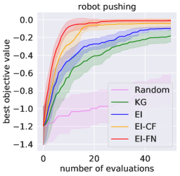
Figure 7: Results from the experiment described in §E.

Appendix F Posterior Mean and Covariance Functions

In this section, we write explicit formulas for the posterior mean and covariance functions of the GP distributions associated to the node functions, $f_{1},\ldots,f_{K}$. To write this more simply, we define some additional notation. Given generic vectors $x\in\mathbb{R}^{D}$ and $y\in\mathbb{R}^{K}$, we define $z_{k}=(x_{I(k)},y_{J(k)})$ as the elements of these vectors supplied as input to node $k$. Similarly, given a historical observation of the values of the node functions $y_{\ell}=(h_{1}(x_{\ell}),\ldots,h_{K}(x_{\ell})),\ \ell=1,\ldots,n$, we define $z_{\ell,k}=(x_{\ell,I(k)},y_{\ell,J(k)})$. Using this notation, our posterior mean and covariance functions can be written as

$$\mu_{n,k}(z_{k})=\mu_{0,k}(z_{k})+\Sigma_{0,k}\left(z_{k},z_{1:n,k}\right)\Sigma_{0,k}\left(z_{1:n,k},z_{1:n,k}\right)^{-1}\left(y_{1:n,k}-\mu_{0,k}\left(z_{1:n,k}\right)\right),$$

and

$$\Sigma_{n,k}(z_{k},z_{k}^{\prime})=\Sigma_{0,k}(z_{k},z_{k}^{\prime})- \Sigma_{0,k}\left(z_{k},z_{1:n,k}\right)\Sigma_{0,k}\left(z_{1:n,k},z_{1:n,k}\right)^{-1}\Sigma_{0,k}\left(z_{1:n,k},z_{k}^{\prime}\right),$$

respectively.

References

- Amaral et al., (2014) Amaral, S., Allaire, D., and Willcox, K. (2014). A decomposition-based approach to uncertainty analysis of feed-forward multicomponent systems. International Journal for Numerical Methods in Engineering, 100(13):982–1005.
- Arcelli, (2020) Arcelli, D. (2020). Exploiting queuing networks to model and assess the performance of self-adaptive software systems: A survey. Procedia Computer Science, 170:498–505.
- Astudillo and Frazier, (2019) Astudillo, R. and Frazier, P. I. (2019). Bayesian optimization of composite functions. In Chaudhuri, K. and Salakhutdinov, R., editors, Proceedings of the 36th International Conference on Machine Learning, volume 97 of Proceedings of Machine Learning Research, pages 354–363. PMLR.
- Astudillo and Frazier, (2021) Astudillo, R. and Frazier, P. I. (2021). Thinking inside the box: A tutorial on grey-box Bayesian optimization. In Proceedings of the 2021 Winter Simulation Conference. Institute of Electrical and Electronics Engineers, Inc.
- Balandat et al., (2020) Balandat, M., Karrer, B., Jiang, D., Daulton, S., Letham, B., Wilson, A. G., and Bakshy, E. (2020). Botorch: A framework for efficient Monte-Carlo Bayesian optimization. In Larochelle, H., Ranzato, M., Hadsell, R., Balcan, M. F., and Lin, H., editors, Advances in Neural Information Processing Systems, volume 33, pages 21524–21538. Curran Associates, Inc.
- Balasubramanian et al., (2020) Balasubramanian, K., Ghadimi, S., and Nguyen, A. (2020). Stochastic multi-level composition optimization algorithms with level-independent convergence rates. arXiv preprint arXiv:2008.10526.
- Bect et al., (2019) Bect, J., Bachoc, F., and Ginsbourger, D. (2019). A supermartingale approach to Gaussian process based sequential design of experiments. Bernoulli, 25(4A):2883–2919.
- Benaouali and Kachel, (2019) Benaouali, A. and Kachel, S. (2019). Multidisciplinary design optimization of aircraft wing using commercial software integration. Aerospace Science and Technology, 92:766–776.
- Bull, (2011) Bull, A. D. (2011). Convergence rates of efficient global optimization algorithms. Journal of Machine Learning Research, 12(88):2879–2904.
- Byrd et al., (1995) Byrd, R. H., Lu, P., Nocedal, J., and Zhu, C. (1995). A limited memory algorithm for bound constrained optimization. SIAM Journal on Scientific Computing, 16(5):1190–1208.
- Cakmak et al., (2020) Cakmak, S., Astudillo Marban, R., Frazier, P., and Zhou, E. (2020). Bayesian optimization of risk measures. In Larochelle, H., Ranzato, M., Hadsell, R., Balcan, M. F., and Lin, H., editors, Advances in Neural Information Processing Systems, volume 33, pages 20130–20141. Curran Associates, Inc.
- Cao et al., (2020) Cao, S., Gan, Y., Wang, C., Bachmann, M., Wei, S., Gong, J., Huang, Y., Wang, T., Li, L., Lu, K., et al. (2020). Post-lockdown sars-cov-2 nucleic acid screening in nearly ten million residents of wuhan, china. Nature communications, 11(1):1–7.
- Charisopoulos et al., (2021) Charisopoulos, V., Chen, Y., Davis, D., Díaz, M., Ding, L., and Drusvyatskiy, D. (2021). Low-rank matrix recovery with composite optimization: Good conditioning and rapid convergence. Foundations of Computational Mathematics, 21(6):1505–1593.
- Çınlar, (2011) Çınlar, E. (2011). Probability and stochastics. Springer.
- Cleary et al., (2021) Cleary, B., Hay, J. A., Blumenstiel, B., Harden, M., Cipicchio, M., Bezney, J., Simonton, B., Hong, D., Senghore, M., Sesay, A. K., et al. (2021). Using viral load and epidemic dynamics to optimize pooled testing in resource-constrained settings. Science Translational Medicine, 13(589):eabf1568.
- Cramer et al., (1994) Cramer, E. J., Dennis, Jr, J. E., Frank, P. D., Lewis, R. M., and Shubin, G. R. (1994). Problem formulation for multidisciplinary optimization. SIAM Journal on Optimization, 4(4):754–776.
- Damianou and Lawrence, (2013) Damianou, A. and Lawrence, N. D. (2013). Deep Gaussian processes. In Carvalho, C. M. and Ravikumar, P., editors, Proceedings of the 16th International Conference on Artificial Intelligence and Statistics, volume 31 of Proceedings of Machine Learning Research, pages 207–215. PMLR.
- Denny et al., (2020) Denny, T. N., Andrews, L., Bonsignori, M., Cavanaugh, K., Datto, M. B., Deckard, A., DeMarco, C. T., DeNaeyer, N., Epling, C. A., Gurley, T., et al. (2020). Implementation of a pooled surveillance testing program for asymptomatic SARS-CoV-2 infections on a college campus — Duke University, Durham, North Carolina, August 2–October 11, 2020. Morbidity and Mortality Weekly Report, 69(46):1743–1747.
- Dorfman, (1943) Dorfman, R. (1943). The detection of defective members of large populations. The Annals of Mathematical Statistics, 14(4):436–440.
- Drusvyatskiy and Paquette, (2019) Drusvyatskiy, D. and Paquette, C. (2019). Efficiency of minimizing compositions of convex functions and smooth maps. Mathematical Programming, 178(1):503–558.
- Frazier, (2018) Frazier, P. I. (2018). A tutorial on Bayesian optimization. arXiv preprint arXiv:1807.02811.
- Frazier et al., (2020) Frazier, P. I., Zhang, Y., and Cashore, M. (2020). Feasibility of COVID-19 screening for the U.S. population with group testing. https://docs.google.com/document/d/1hw5K5V7XOug_r6CQ0UYt25szQxXFPmZmFhK15ZpH5U0/edit?ts=5e934170#.
- Fu and Henderson, (2017) Fu, M. C. and Henderson, S. G. (2017). History of seeking better solutions, AKA simulation optimization. In Chan, W. K. V., D’Ambrogio, A., Zacharewicz, G., N. Mustafee, G. W., and Page, E., editors, Proceedings of the 2017 Winter Simulation Conference, pages 131–157. Institute of Electrical and Electronics Engineers, Inc.
- Garnett, (2002) Garnett, G. P. (2002). An introduction to mathematical models in sexually transmitted disease epidemiology. Sexually transmitted infections, 78(1):7–12.
- Ghasemi et al., (2018) Ghasemi, A., Heavey, C., and Laipple, G. (2018). A review of simulation-optimization methods with applications to semiconductor operational problems. In Rabe, M., Juan, A. A., Mustafee, N., Skoogh, A., Jain, S., and Johansson, B., editors, Proceedings of the 2018 Winter Simulation Conference, pages 3672–3683. Institute of Electrical and Electronics Engineers, Inc.
- Hansen, (2016) Hansen, N. (2016). The CMA evolution strategy: A tutorial. arXiv preprint arXiv:1604.00772.
- Hattrick-Simpers et al., (2016) Hattrick-Simpers, J. R., Gregoire, J. M., and Kusne, A. G. (2016). Perspective: Composition–structure–property mapping in high-throughput experiments: Turning data into knowledge. APL Materials, 4(5):053211.
- Homem-de Mello, (2008) Homem-de Mello, T. (2008). On rates of convergence for stochastic optimization problems under non-independent and and identically distributed sampling. SIAM Journal on Optimization, 19(2):524–551.
- Jamil and Yang, (2013) Jamil, M. and Yang, X.-S. (2013). A literature survey of benchmark functions for global optimization problems. arXiv preprint arXiv:1308.4008.
- Jones et al., (1998) Jones, D. R., Schonlau, M., and Welch, W. J. (1998). Efficient global optimization of expensive black-box functions. Journal of Global Optimization, 13(4):455–492.
- Kandasamy et al., (2017) Kandasamy, K., Dasarathy, G., Schneider, J., and Póczos, B. (2017). Multi-fidelity Bayesian optimisation with continuous approximations. In Precup, D. and Teh, Y. W., editors, Proceedings of the 34th International Conference on Machine Learning, volume 70 of Proceedings of Machine Learning Research, pages 1799–1808. PMLR.
- Kleywegt et al., (2002) Kleywegt, A. J., Shapiro, A., and Homem-de Mello, T. (2002). The sample average approximation method for stochastic discrete optimization. SIAM Journal on Optimization, 12(2):479–502.
- Li et al., (2021) Li, H., Zhao, G., Johari, R., and Weintraub, G. Y. (2021). Interference, bias, and variance in two-sided marketplace experimentation: Guidance for platforms. arXiv preprint arXiv:2104.12222.
- Lizotte et al., (2007) Lizotte, D. J., Wang, T., Bowling, M. H., and Schuurmans, D. (2007). Automatic gait optimization with Gaussian process regression. In Proceedings of the 20th International Joint Conference on Artificial Intelligence, pages 944–949.
- Marque-Pucheu et al., (2019) Marque-Pucheu, S., Perrin, G., and Garnier, J. (2019). Efficient sequential experimental design for surrogate modeling of nested codes. ESAIM: PS, 23:245–270.
- Močkus, (1975) Močkus, J. (1975). On Bayesian methods for seeking the extremum. In Marchuk, G. I., editor, Optimization Techniques IFIP Technical Conference, volume 27 of Lecture Notes in Computer Science, pages 400–404. Springer-Verlag.
- Osorio and Bierlaire, (2013) Osorio, C. and Bierlaire, M. (2013). A simulation-based optimization framework for urban transportation problems. Operations Research, 61(6):1333–1345.
- Plappert et al., (2018) Plappert, M., Andrychowicz, M., Ray, A., McGrew, B., Baker, B., Powell, G., Schneider, J., Tobin, J., Chociej, M., Welinder, P., et al. (2018). Multi-goal reinforcement learning: Challenging robotics environments and request for research. arXiv preprint arXiv:1802.09464.
- Puterman, (1990) Puterman, M. L. (1990). Markov decision processes. In Stochastic Models, volume 2 of Handbooks in Operations Research and Management Science, pages 331–434. Elsevier.
- Rasmussen and Williams, (2006) Rasmussen, C. E. and Williams, C. K. I. (2006). Gaussian processes for machine learning. MIT Press.
- Ryzhov, (2016) Ryzhov, I. O. (2016). On the convergence rates of expected improvement methods. Operations Research, 64(6):1515–1528.
- Sadowski and Jones, (2009) Sadowski, M. and Jones, D. (2009). The sequence–structure relationship and protein function prediction. Current Opinion in Structural Biology, 19(3):357–362.
- Sandberg, (1978) Sandberg, I. (1978). On the mathematical foundations of compartmental analysis in biology, medicine, and ecology. IEEE transactions on Circuits and Systems, 25(5):273–279.
- Sekhon and Saluja, (2011) Sekhon, B. S. and Saluja, V. (2011). Biosimilars: An overview. Biosimilars, 1(1):1–11.
- Shahriari et al., (2016) Shahriari, B., Swersky, K., Wang, Z., Adams, R. P., and De Freitas, N. (2016). Taking the human out of the loop: A review of Bayesian optimization. Proceedings of the IEEE, 104(1):148–175.
- Shapiro, (2003) Shapiro, A. (2003). On a class of nonsmooth composite functions. Mathematics of Operations Research, 28(4):677–692.
- Snoek et al., (2012) Snoek, J., Larochelle, H., and Adams, R. P. (2012). Practical Bayesian optimization of machine learning algorithms. In Pereira, F., Burges, C. J. C., Bottou, L., and Weinberger, K. Q., editors, Advances in Neural Information Processing Systems, volume 25, pages 2951–2959. Curran Associates, Inc.
- Surjanovic and Bingham, (2013) Surjanovic, S. and Bingham, D. (2013). Drop-Wave function.
- Sutton and Barto, (2018) Sutton, R. S. and Barto, A. G. (2018). Reinforcement learning: An introduction. MIT press.
- Swersky et al., (2013) Swersky, K., Snoek, J., and Adams, R. P. (2013). Multi-task Bayesian optimization. In Burges, C. J. C., Bottou, L., Welling, M., Ghahramani, Z., and Weinberger, K. Q., editors, Advances in Neural Information Processing Systems, volume 26, pages 2004–2012. Curran Associates, Inc.
- Toscano-Palmerin and Frazier, (2018) Toscano-Palmerin, S. and Frazier, P. I. (2018). Bayesian optimization with expensive integrands. arXiv preprint arXiv:1803.08661.
- Uhrenholt and Jensen, (2019) Uhrenholt, A. K. and Jensen, B. S. (2019). Efficient Bayesian optimization for target vector estimation. In Chaudhuri, K. and Sugiyama, M., editors, Proceedings of the 22nd International Conference on Artificial Intelligence and Statistics, volume 89 of Proceedings of Machine Learning Research, pages 2661–2670. PMLR.
- Vazquez and Bect, (2010) Vazquez, E. and Bect, J. (2010). Convergence properties of the expected improvement algorithm with fixed mean and covariance functions. Journal of Statistical Planning and Inference, 140(11):3088–3095.
- Wang et al., (2020) Wang, X., Gong, X., Geng, N., Jiang, Z., and Zhou, L. (2020). Metamodel-based simulation optimisation for bed allocation. International Journal of Production Research, 58(20):6315–6335.
- Wang and Jegelka, (2017) Wang, Z. and Jegelka, S. (2017). Max-value entropy search for efficient Bayesian optimization. In Precup, D. and Teh, Y. W., editors, Proceedings of the 34th International Conference on Machine Learning, volume 70 of Proceedings of Machine Learning Research, pages 3627–3635. PMLR.
- Westreich et al., (2008) Westreich, D. J., Hudgens, M. G., Fiscus, S. A., and Pilcher, C. D. (2008). Optimizing screening for acute human immunodeficiency virus infection with pooled nucleic acid amplification tests. Journal of Clinical Microbiology, 46(5):1785–1792.
- Williams et al., (2000) Williams, B. J., Santner, T. J., and Notz, W. I. (2000). Sequential design of computer experiments to minimize integrated response functions. Statistica Sinica, 10(4):1133–1152.
- Wilson et al., (2018) Wilson, J., Hutter, F., and Deisenroth, M. (2018). Maximizing acquisition functions for bayesian optimization. In Bengio, S., Wallach, H., Larochelle, H., Grauman, K., Cesa-Bianchi, N., and Garnett, R., editors, Advances in Neural Information Processing Systems, volume 31, pages 9884–9895. Curran Associates, Inc.
- Wu and Frazier, (2016) Wu, J. and Frazier, P. (2016). The parallel knowledge gradient method for batch Bayesian optimization. In Lee, D., Sugiyama, M., Luxburg, U., Guyon, I., and Garnett, R., editors, Advances in Neural Information Processing Systems, volume 29, pages 3134–3142. Curran Associates, Inc.
- Wu et al., (2019) Wu, J., Toscano-Palmerin, S., Frazier, P. I., and Wilson, A. G. (2019). Practical multi-fidelity Bayesian optimization for hyperparameter tuning. In Proceedings of the 35th Conference on Uncertainty in Artificial Intelligence.
- Zhilinskas, (1975) Zhilinskas, A. (1975). Single-step Bayesian search method for an extremum of functions of a single variable. Cybernetics, 11(1):160–166.