Spin-injection-generated shock waves and solitons in a ferromagnetic thin film: the spin piston problem

Abstract

The unsteady, nonlinear magnetization dynamics induced by spin injection in an easy-plane ferromagnetic channel subject to an external magnetic field are studied analytically. Leveraging a dispersive hydrodynamic description, the Landau-Lifshitz equation is recast in terms of hydrodynamic-like variables for the magnetization’s perpendicular component (spin density) and azimuthal phase gradient (fluid velocity). Spin injection acts as a moving piston that generates nonlinear, dynamical spin textures in the ferromagnetic channel with downstream quiescent spin density set by the external field. In contrast to the classical problem of a piston accelerating a compressible gas, here, variable spin injection and field lead to a rich variety of nonlinear wave phenomena from oscillatory spin shocks to solitons and rarefaction waves. A full classification of solutions is provided using nonlinear wave modulation theory by identifying two key aspects of the fluid-like dynamics: subsonic/supersonic conditions and convex/nonconvex hydrodynamic flux. Familiar waveforms from the classical piston problem such as rarefaction (expansion) waves and shocks manifest in their spin-based counterparts as smooth and highly oscillatory transitions, respectively, between two distinct magnetic states. The spin shock is an example of a dispersive shock wave, which arises in many physical systems. New features without a gas dynamics counterpart include composite wave complexes with "contact” spin shocks and rarefactions. Magnetic supersonic conditions lead to two pronounced piston edge behaviors including a stationary soliton and an oscillatory wavetrain. These coherent wave structures have physical implications for the generation of high frequency spin waves from pulsed injection and persistent, stable stationary and/or propagating solitons in the presence of magnetic damping. The analytical results are favorably compared with numerical simulations.

I Introduction

Spin transport in magnetic materials has been intensely studied, due, in part, to its potential spintronic applications in information technology. A promising means for long-distance transport of angular momentum is by way of large-amplitude, fluid-like excitations [1, 2]. A useful approach to study these nonlinear spin dynamics is the hydrodynamic framework. First proposed by Halperin and Hohenberg [3] to describe spin waves in anisotropic ferro- and antiferromagnets under long-wavelength assumptions, the hydrodynamic perspective—essentially a transformation of the Landau-Lifshitz equation to a set of fluid-like variables—has since been utilized by a number of researchers to investigate a variety of novel spin textures and dynamics, sometimes referred to as superfluid spin transport [4, 5, 6, 7, 8, 9, 10, 11, 12, 13]. Actually, magnetic damping implies energy dissipation, which must be compensated if sustained superfluid-like spin states are desired. An adequate compensation mechanism is the injection of spin into material boundaries via the spin-Hall effect, spin-transfer torque [6, 7, 8, 14, 15, 10], or the quantum spin-Hall effect [16]. Recent experimental observations of superfluid-like spin transport indicate that such dynamics are possible [14, 16].

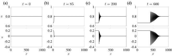
Figure 1: Temporal development of a spin shock (DSW) solution to the piston problem in a 1D easy-plane ferromagnetic channel. (a) Initial state prior to spin piston acceleration with constant spin density $n=h_{0}=0.8$ and fluid velocity $u=0$. (b) The piston velocity accelerates to $99.9\%$ of $u_{0}=0.2$ leading to a compressive wave. (c) A spin shock is under development. (d) A spin shock is fully developed.

The analytical study of fluid-like spin transport in ferromagnetic materials can be conveniently formulated in terms of dispersive hydrodynamics (DH) in which large scale, nonlinear wave motion in a dispersive medium is described by conservation laws subject to dispersive corrections [17]. Just such a DH formulation of magnetization dynamics was proposed in [8] as an exact transformation of the Landau-Lifshitz (LL), a standard continuum, micromagnetic model of ferromagnetic materials. It recasts the three-component magnetization vector $\mathbf{m}=(m_{x},m_{y},m_{z})$, constrained to normalized unit length, in terms of two dependent variables: the longitudinal spin density $n=m_{z}$ and the fluid velocity $\mathbf{u}=-\nabla\arctan(m_{y}/m_{x})$. The latter is proportional to the longitudinal component of the spin current. Since $m_{y},m_{x}\to 0$ when $m_{z}\to\pm 1$, $\mathbf{u}$ is undefined when the magnetization is saturated in the perpendicular direction so this is referred to as the vacuum state. When the local fluid speed exceeds the critical value $u_{\rm cr}=\sqrt{(1-n^{2})/(1+3n^{2})}$ (different from the local speed of sound due to broken Galilean invariance), the flow can be understood as supersonic [8], resulting, for example, in the generation of magnetic vortices and antivortices with vacuum states at their core [18, 19]. Since the transformation is exact, the DH formulation captures all of the essential physics that are involved: exchange, anisotropy, and damping, manifesting as dispersion, nonlinearity, and viscous effects, respectively. Under conditions in which anisotropy and exchange dominate, such as when the spin density exhibits a large gradient, the spin system can develop rapidly oscillatory structures including solitons and spin shocks, also known as dispersive shock waves (DSWs), observed in the envelope of magnetostatic spin waves in Yttrium Iron Garnet films [20]. Such DSWs are known to occur in a variety of other DH media including Bose-Einstein condensates (BECs) [21], nonlinear spatial [22] and fiber [23] optics, and fluid dynamics [24, 25]. Highly oscillatory, unsteady DSWs contrast sharply with nonlinear, dissipation-dominated, non-oscillatory, steady shock waves in other systems such as a compressible gas [26].

With the DH interpretation of spin dynamics in mind, we will focus on the analytical study of the canonical problem of spin injection into an easy-plane ferromagnet as a feasible mechanism to generate large-amplitude, unsteady spin textures with fluid-like features. This problem was recently considered by us in [12] by way of numerical simulations of the LL equation. We showed that the presence of a perpendicular, uniform, external magnetic field and the rapid onset of spin injection resulted in three evolutionary stages: 1) injection rise leading to the generation of fluid-like expansion and/or compression waves, 2) pre-relaxation in which the dynamics are dominated by exchange and anisotropy resulting in rarefaction and shock waves, and 3) relaxation to steady state where damping, exchange and anisotropy result in steady, precessional dissipative exchange flows [10], also known as spin superfluids [5, 6].

In the present work, we focus on the pre-relaxation stage where magnetic damping is negligible relative to exchange and anisotropy. We interpret spin injection at one material boundary as a “spin piston” whose resultant spin current is analogous to the piston velocity. The rapid onset of spin injection causes the acceleration of the spin piston, which in turn leads to the development of a large spin density gradient in the sample. Such conditions result in dispersive hydrodynamics. The piston drives fluid-like excitations into an otherwise static magnetic configuration whose spin density is determined by a perpendicular external magnetic field. Different spin injection and field strengths lead to a variety of spin rarefaction waves, spin shocks, and solitons.

The development of a spin shock generated by the spin piston is shown in Fig. 1. As demonstrated in [12], by considering the problem on short enough time scales, we can neglect magnetic damping. Therefore, in this work, we use nonlinear wave/Whitham modulation theory [27, 28, 17] to analytically classify the dynamic spin textures generated by the spin piston with fixed velocity $u_{0}$ and field $h_{0}$ with negligible damping. Our primary result is the phase diagram depicting the various solution types in the injection-field ($u_{0}$-$h_{0}$) plane of Fig. 2. This diagram demonstrates the rich selection of fluid-like spin textures that can be generated in this system. Moreover, these dispersive hydrodynamic waves have physical implications for the generation of spin waves from pulsed injection and stable solitons coincident with dissipative exchange flows.

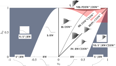
Figure 2: Classification of spin piston dynamics in terms of the piston velocity $u_{0}$ (spin injection) and background spin density $h_{0}$ (external magnetic field). The acronyms used in the Figure and throughout the text are defined in Table 1. Dotted black curve: divide between convex (left) and nonconvex (right) regimes. Solid black lines: $r_{+}^{L}=r_{+}^{R}$ (see main text). The pink-shaded region implies the existence of the vacuum state $|n|=1$ within the oscillatory solution. The subsonic regime is identified in white. Sector I: $\mathrm{RW}$; Sector II: $\mathrm{DSW}^{+}$; Sector III: $\mathrm{DSW}^{+}\mathrm{CDSW}^{+}$; Boundary $\textup{III}/\textup{IV}$ between sector III and IV: $\mathrm{CDSW}$; Sector IV: $\mathrm{RW}\,\mathrm{CDSW}^{+}$. The supersonic regime is in the gray, shaded region. Sector V: $\mathrm{S}^{+}|\mathrm{RW}$, supersonic condition $v_{-}<v_{+}<0$; Sector VI: $\mathrm{S}^{-}|\mathrm{RW}\,\mathrm{CDSW}^{+}$, supersonic condition $v_{-}<v_{+}<0$; Sector VII: $\mathrm{PDSW}^{+}|\mathrm{DSW}^{+}$, supersonic condition $0<v_{-}<v_{+}$.

In addition to the piston problem, another canonical hydrodynamic problem is the space-time evolution of an initial, sharp gradient, known as the Riemann problem [29]. We highlight the work of [30] in which the Riemann problem for polarization waves in a two-component BEC is classified. As it turns out, the governing equations studied there are equivalent to the LL equation in one spatial dimension that we study here in dispersive hydrodynamic form absent magnetic damping. As such, we rely heavily upon the analysis carried out in [30]. Nevertheless, the piston problem studied here introduces new boundary effects that do not occur in Riemann problems such as supersonic flow conditions that generate a soliton attached to the piston or a partial DSW that emanates from it. Moreover, the spin piston problem is a physically plausible setting to generate spin shocks and other dispersive hydrodynamic spin textures in magnetic materials.

Table 1: List of acronyms and symbols.

RW	rarefaction wave
DSW	dispersive shock wave
CDSW	contact dispersive shock wave
PDSW	partial dispersive shock wave
S	soliton
|	constant plateau separating waves
$\pm$ superscripts	$+$: elevation soliton, $-$: depression soliton

Related superfluid and superfluid-like piston problems have been studied theoretically [31, 32] and experimentally [33, 34] in BECs and optics. While they reveal intriguing dispersive hydrodynamic features such as the generation of an oscillatory wake at the piston accompanied by vacuum points [31, 34], there are a number of new effects predicted by the spin piston problem studied here. This is because the hydrodynamic flux of the spin system is nonconvex whereas the flux in BEC and optics is convex. Nonconvexity manifests in the spin analogues of conservation of mass and momentum with non-monotonic hydrodynamic fluxes are in the spin density and fluid velocity. Mathematically, the long-wavelength hydrodynamic system loses strict hyperbolicity and/or genuine nonlinearity. This leads to new types of dispersive hydrodynamics [35]. In addition to expanding rarefaction waves (RWs) and compressive DSWs in Figures 1 and 2, nonconvexity results in hybrid spin textures composed of a RW and a special kind of contact spin shock or contact DSW (CDSW)—the dispersive hydrodynamic analogue of a contact discontinuity in gas dynamics—whose velocity coincides with a long wavelength magnetic speed of sound. Table 1 lists the acronyms and symbols used throughout the main text and in Fig. 2. We identify the supersonic transition at the piston as coincident with either the rapid generation of a stationary soliton or a partial DSW. Finally, sufficiently large external field and positive piston velocity result in the generation of vacuum points within the oscillatory solution. Although we focus on the early, dissipationless spin dynamics, each of these distinct dispersive hydrodynamic excitations have implications for the long-time, steady-state evolution of the spin system subject to magnetic damping [12]. These implications are discussed in our concluding remarks Section VIII.

Table 2: Physical and mathematical properties of the solution sectors in the phase diagram of Fig. 2.

I: RW	subsonic, expansive, convex
II: DSW+	subsonic, compressive, convex
III: DSW+ CDSW+	subsonic, compressive, nonconvex
IV: RW CDSW+	subsonic, expansive/compressive, nonconvex
V: S+|RW	supersonic, expansive, convex
VI: S-|RW CDSW+	supersonic, expansive/compressive, nonconvex
VII: PDSW+|DSW+	supersonic, compressive, convex/nonconvex

The rest of the paper is organized as follows. Section II describes the spin piston problem setup. Section III provides a summary of the results of Whitham modulation theory from [30] so that the analysis is self-contained. Some additional analytical details are provided in the Appendix. In Section V, solutions with zero applied field are presented and analyzed in both the subsonic and supersonic regimes. In Sections VI and VII, solutions arising in the presence of a uniform perpendicular applied field are analyzed in the subsonic and supersonic regimes, respectively. Finally, we present the conclusion in Section VIII.

II Model

Consider a one-dimensional, easy-plane ferromagnetic channel oriented in the $\hat{\mathbf{x}}$ direction with length $L$. Spin injection is applied to the left edge where $x=0$. The right edge at $x=L$ corresponds to a free spin boundary. The governing equation is the non-dimensional, dissipationless LL equation, given by

$$\partial_{t}\mathbf{m}=-\mathbf{m}\crossproduct\mathbf{h}_{\mathrm{eff}},\quad x\in(0,L),t>0,$$ (1)

where

$$\mathbf{h}_{\mathrm{eff}}=\partial_{xx}\mathbf{m}-m_{z}\hat{\mathbf{z}}+h_{0}\hat{\mathbf{z}}.$$ (2)

Here, $\mathbf{m}=\mathbf{M}/M_{s}=(m_{x},m_{y},m_{z})$ is the normalized magnetization vector, and $M_{s}$ is the saturation magnetization. The effective field (2) is also normalized by $M_{s}$ and consists of exchange, easy-plane anisotropy, and a uniform externally applied magnetic field with constant magnitude $h_{0}$ along the perpendicular-to-plane ($\hat{\mathbf{z}}$) direction. The non-dimensionalization leading to Eq. (1) is achieved by scaling time by $|\gamma|\mu_{0}M_{s}$ and space by $\lambda_{\mathrm{ex}}^{-1}$, where $\gamma$ is the gyromagnetic ratio, $\mu_{0}$ is the vacuum permeability, and $\lambda_{\mathrm{ex}}$ is the exchange length. The dissipationless LL serves as a valid model here considering the timescale within which damping is not a key factor in the development of the dynamical structures [12]. We will discuss the role of damping on longer time scales in the conclusion.

The following analysis is based on the DH formulation of Eq. (1) in terms of the hydrodynamic variables

$$\text{spin density: }n =m_{z},$$

$$\text{fluid velocity: }u =-\partial_{x}\Phi=-\partial_{x}\arctan(m_{y}/m_{x}),$$

where $\Phi$ is the azimuthal phase angle. The DH formulation is given by [18]

$$\partial_{t}n =\partial_{x}\left[(1-n^{2})u\right],$$ (3a)

$$\partial_{t}u =\partial_{x}\left[(1-u^{2})n\right]-\partial_{x}\left(\frac{\partial_{xx}n}{1-n^{2}}-\frac{n(\partial_{x}n)^{2}}{(1-n^{2})^{2}}\right),$$ (3b)

$$\partial_{t}\Phi =h_{0}-(1-u^{2})n+\frac{1}{\sqrt{1-n^{2}}}\partial_{x}\left(\frac{\partial_{x}n}{\sqrt{1-n^{2}}}\right),$$ (3c)

where (3b) follows from the negative gradient of (3c). These equations result from an exact transformation of the LL equation (1). Equation (3) is analogous to the mass, momentum, and Bernoulli equations for an inviscid, irrotational, compressible fluid. Owing to a phase singularity, the vacuum state occurs when $|n|=1$. Equation (3) is invariant to the reflection transformation

$$h_{0}\to-h_{0},\quad n\to-n,\quad\Phi\to-\Phi,\quad u\to-u.$$ (4)

The boundary conditions (BCs) for Eq. (3) are

$$\partial_{x}n(0,t)=0,\quad \partial_{x}n(L,t)=0,$$ (5a)

$$u(0,t)=u_{b}(t),\quad u(L,t)=0,$$ (5b)

where $u_{b}(t)$ models the time dependence of a perfect spin injection source that increases from 0 to the maximum intensity $|u_{0}|$ monotonically and smoothly with the rise time $t_{0}$. We adopt a hyperbolic tangent profile to model the injection rise: $u(0,t)=(u_{0}/2)\{\tanh[(t-t_{0}/2)/(t_{0}/10)]+1\}$, where $t_{0}=80$ is the time that the injection magnitude reaches $99.99\%$ of $|u_{0}|$. For a typical Permalloy, this hyperbolic tangent profile produces a relatively sharp change in the hydrodynamic variables—about $2$ ns—when compared to the typical precessional period of spin-injected DEFs, on the order of 10–20 ns [9]. The modulationally stable region, consisting of velocities $u$ in the interval $[-1,1]$, corresponds to stable fluid-like configurations, so we restrict $|u_{0}|<1$ [8]. The initial condition (IC) is given by

$$n(x,t=0) =h_{0},$$ (6a)

$$u(x,t=0) =0,$$ (6b)

with $|h_{0}|<1$. Thus, the spin injection problem can be reduced to a piston problem: a piston at $x=0$, initially with velocity $u=0$, is accelerated to $u=u_{0}$, generating a flow to the right ($u_{0}>0$) or left ($u_{0}<0$) into the quiescent fluid with density $n=h_{0}$. In the rest of this work, we will refer to this piston analogy for our interpretation of the spin dynamics that result from the initial-boundary value problem (3)–(6). We focus on the classification of solutions when they are fully developed such as in Fig. 1(d).

III Nonlinear Wave Dynamics and Whitham Modulation Theory

In this section, we provide some necessary background, primarily following [30], on Whitham modulation theory, a powerful tool for studying multiscale nonlinear wave dynamics [27, 28, 17]. Modulation theory results in equations that describe the slow variation of nonlinear, periodic traveling wave solutions.

III.1 Traveling Wave Solutions

Consider the traveling wave solutions of Eq. (3) in the form $n(x,t)=n(\xi)$ and $u(x,t)=u(\xi)$ with the moving coordinate $\xi=x-Vt$, where

$$V^{2}=\frac{1}{2}\left(1+\sum_{i<j}^{4}n_{i}n_{j}+\prod_{i}^{4}n_{i}+\sqrt{\prod_{i}^{4}(1-n_{i}^{2})}\right)$$ (7)

is the square of the wave’s phase speed and $n_{i}$, $i=1,2,3,4$ are wave parameters. The positive/negative square root corresponds to right/left-going wave solutions, respectively. By insertion of $n(\xi)$, $u(\xi)$ into (3) and direct integration, the traveling wave satisfies the ordinary differential equation (ODE)

$$\left(\frac{dn}{d\xi}\right)^{2}=-R(n),$$ (8)

where $R(n)=(n-n_{1})(n-n_{2})(n-n_{3})(n-n_{4})$ is the potential function, a quartic polynomial with zeros at $n_{i}$, $i=1,2,3,4$. The velocity field $u(\xi)$ can be obtained in terms of $n(\xi)$ and the roots $n_{i}$ [30] so we focus on the modulation analysis with $n$. For real, ordered $n_{1}\leq n_{2}\leq n_{3}\leq n_{4}$ in the interval $[-1,1]$, the traveling wave solution for $n$ either oscillates within $[n_{1},n_{2}]$ or $[n_{3},n_{4}]$ with wavelength given by

$$L=\frac{4K(m)}{\sqrt{(n_{3}-n_{1})(n_{4}-n_{2})}},$$ (9)

where $K(m)$ is the complete elliptic integral of the first kind with $m$ given by

$$m=\frac{(n_{4}-n_{3})(n_{2}-n_{1})}{(n_{4}-n_{2})(n_{3}-n_{1})}.$$ (10)

When $n$ oscillates within $[n_{1},n_{2}]$, the traveling wave solution is

$$n(\xi)=n_{2}-\frac{(n_{2}-n_{1})\mathrm{cn}^{2}(W,m)}{1+\frac{n_{2}-n_{1}}{n_{4}-n_{2}}\mathrm{sn}^{2}(W,m)},$$ (11)

where

$$W=\sqrt{(n_{3}-n_{1})(n_{4}-n_{2})}\xi/2$$ (12)

and $\mathrm{cn}$, $\mathrm{sn}$ are Jacobi elliptic functions [36]. The velocity is given in terms of $n$ by

$$u=-\frac{A_{1}+Vn}{1-n^{2}},$$ (13)

where

$$A_{1}^{2} =\frac{1}{2}\left(1+\sum_{i<j}^{4}n_{i}n_{j}+\prod_{i}^{4}n_{i}\mp\prod_{i}^{4}\sqrt{1-n_{i}^{2}}\right),$$ (14)

$$V =\sqrt{\frac{1}{2}\left(1+\displaystyle\sum_{i<j}^{4}n_{i}n_{j}+\prod_{i}^{4}n_{i}\pm\prod_{i}^{4}\sqrt{1-n_{i}^{2}}\right)}.$$

The positive square root of $A_{1}$ is taken here. The upper (lower) sign in (14) gives the fast (slow) branch of wave. $V$ in Eq. (7) is the fast branch. We can also describe the solution in terms of an alternative set of physical wave parameters $(\bar{n},\bar{u},a,k)$, equivalent to $n_{i}$, corresponding to the mean spin density $\bar{n}$, mean velocity $\bar{u}$, the amplitude $a=n_{2}-n_{1}$, and the wavenumber $k=2\pi/L$.

When $n_{3}\rightarrow n_{2}$ and $m\rightarrow 1$, the solution limits to a depression soliton

$$n=n_{2}-\frac{n_{2}-n_{1}}{\cosh^{2}W+\frac{n_{2}-n_{1}}{n_{4}-n_{2}}\sinh^{2}W},$$ (15)

with background mean density $\bar{n}=n_{2}$. The fluid velocity in the soliton limit is

$$u=-\frac{B+c_{s}n}{1-n^{2}},$$ (16)

where

$$\begin{split}B&=\bar{u}(\bar{n}^{2}-a\bar{n}+1)+\bar{n}\mu,\\ c_{s}&=\bar{u}(2\bar{n}-a)+\mu,\\ \mu&=\pm\sqrt{(1-(\bar{n}-a)^{2})(1-\bar{u}^{2})},\end{split}$$ (17)

where $c_{s}$ is the soliton speed and $\bar{u}$ is the background mean velocity. The sign $+$($-$) gives the fast (slow) soliton. In terms of the roots $\{n_{i}\}_{i=1}^{4}$, $c_{s}$ and $\bar{u}$ for the soliton can be obtained by taking the limit $n_{3}\rightarrow n_{2}$ in (13) and (14).

When $n_{4}\to n_{3}$, $m\to 0$, there are two possible limiting solutions. If $n_{2}-n_{1}\ll n_{3}-n_{1}$, then the solution limits to a small-amplitude harmonic wave. If $n_{2}\rightarrow n_{3}=n_{4}$, the solution limits to a depression algebraic soliton

$$n(x,t)=n_{2}-\frac{n_{2}-n_{1}}{1+\frac{1}{4}(n_{2}-n_{1})^{2}\xi^{2}}.$$ (18)

The background mean density for the algebraic soliton is $\bar{n}=n_{2}=n_{3}=n_{4}$. The algebraic soliton amplitude is $a=n_{2}-n_{1}$. The background mean velocity $\bar{u}$ and algebraic soliton speed are obtained by setting $n_{2}=n_{3}=n_{4}$ in (13) and (14).

When $n$ oscillates within $[n_{3},n_{4}]$, the traveling wave solution is

$$n(\xi)=n_{3}+\frac{(n_{4}-n_{3})\mathrm{cn}^{2}(W,m)}{1+\frac{n_{4}-n_{3}}{n_{3}-n_{1}}\mathrm{sn}^{2}(W,m)},$$ (19)

where $W$ is given in (12). The velocity is (13) with $A_{1}$ taking the negative square root and the same $V$ in (14).

When $n_{3}\rightarrow n_{2}$ and $m\rightarrow 1$, the solution limits to an elevation soliton

$$n=n_{3}+\frac{n_{4}-n_{3}}{\cosh^{2}W+\frac{n_{4}-n_{3}}{n_{3}-n_{1}}\sinh^{2}W}.$$ (20)

The background mean density for the soliton is $\bar{n}=n_{2}=n_{3}$. The soliton amplitude is $a=n_{4}-n_{3}$. The background mean velocity $\bar{u}$ is obtained by taking the limit $n_{3}\rightarrow n_{2}$ in (13) and (14). Alternatively, the fluid velocity in the soliton limit is (16) with

$$\begin{split}B&=\bar{u}(\bar{n}^{2}+a\bar{n}+1)+\bar{n}\mu,\\ c_{s}&=\bar{u}(2\bar{n}+a)+\mu,\\ \mu&=\pm\sqrt{(1-(\bar{n}+a)^{2})(1-\bar{u}^{2})},\end{split}$$ (21)

where $+$($-$) gives the fast (slow) soliton.

When $n_{2}\to n_{1}$, $m\to 0$, there are two possible limiting solutions. If $n_{4}-n_{3}\ll n_{4}-n_{1}$, then the solution limits to a small-amplitude harmonic wave. If $n_{3}\rightarrow n_{2}=n_{1}$, the solution limits to an elevation algebraic soliton

$$n(x,t)=n_{3}+\frac{n_{4}-n_{3}}{1+\frac{1}{4}(n_{4}-n_{3})^{2}\xi^{2}}.$$ (22)

The background mean density for the algebraic soliton is $\bar{n}=n_{3}=n_{2}=n_{1}$ and the soliton amplitude is $a=n_{4}-n_{3}$. The background mean velocity $\bar{u}$ and algebraic soliton speed are obtained by setting $n_{1}=n_{2}=n_{3}$ in (13) and (14).

III.2 Whitham Modulation Equations

The modulation equations can be expressed in diagonal form by introducing new modulation variables $\lambda_{i}$ known as Riemann invariants

$$\frac{\partial\lambda_{i}}{\partial t}+v_{i}\frac{\partial\lambda_{i}}{\partial x}=0,\quad i=1,2,3,4,$$ (23)

where the Riemann invariants are ordered as $\lambda_{1}\leq\lambda_{2}\leq\lambda_{3}\leq\lambda_{4}$, and the $v_{i}$ are the Whitham velocities

$$v_{i}=\frac{1}{2}\sum_{i=1}^{4}\lambda_{i}-\frac{L}{2\partial L/\partial\lambda_{i}},\quad i\in{1,2,3,4},$$ (24)

where $L=\frac{4K(m)}{\sqrt{(\lambda_{3}-\lambda_{1})(\lambda_{4}-\lambda_{2})}}$ and $m=\frac{(\lambda_{4}-\lambda_{3})(\lambda_{2}-\lambda_{1})}{(\lambda_{4}-\lambda_{2})(\lambda_{3}-\lambda_{1})}$. The transformation between the $n_{i}$ and $\lambda_{i}$ is provided in the Appendix.

The LL-Whitham modulation equations (23) are nonconvex, namely they can lose strict hyperbolicity (two Whitham velocities coalesce) and/or they can lose genuine nonlinearity where $\frac{\partial v_{i}}{\partial\lambda_{i}}=0$ in certain parameter regimes, resulting in a nonmonotonic dependence of the Whitham velocity on the Riemann invariant.

III.3 Piston Sonic and Convexity Conditions

The modulation equations (23) exhibit two important limiting simplifications. By comparing (9) and (10), we find that the soliton limit ($L\to\infty$ and $m\to 1$) occurs when $\lambda_{2}\to\lambda_{3}$ and the spin wave harmonic limit ($a\to 0$ and $m\to 0$) occurs when either $\lambda_{1}\to\lambda_{2}$ or $\lambda_{3}\to\lambda_{4}$. In these limits, two of the modulation equations coincide with the long-wave, dispersionless limit of Eqs. (3a) (3b)

$$\partial_{t}\bar{n} =\partial_{x}\left[(1-\bar{n}^{2})\bar{u}\right],$$ (25a)

$$\partial_{t}\bar{u} =\partial_{x}\left[(1-\bar{u}^{2})\bar{n}\right].$$ (25b)

The remaining two modulation equations merge and correspond to modulations of either the soliton amplitude or the spin wave wavenumber. The limiting velocities determine the motion of DSW edges. In the soliton limit, we have

$$s_{-}\equiv\lim_{\lambda_{2}\to\lambda_{3}}v_{2}=\lim_{\lambda_{2}\to\lambda_{3}}v_{3}=\tfrac{1}{2}(\lambda_{1}+2\lambda_{3}+\lambda_{4}).$$ (26)

In one of the harmonic limits, we have

$$s_{+}\equiv\lim_{\lambda_{3}\to\lambda_{4}}v_{3}=\lim_{\lambda_{3}\to\lambda_{4}}v_{4}=2\lambda_{4}+\frac{(\lambda_{2}-\lambda_{1})^{2}}{2(\lambda_{1}+\lambda_{2}-2\lambda_{4})}.$$ (27)

The velocities $s_{-}<s_{+}$ are the trailing and leading edges of the DSW.

The dispersionless equations (25) describe the evolution of the mean density $\bar{n}$ and mean velocity $\bar{u}$. These equations can be expressed in diagonal form

$$\frac{\partial r_{\pm}}{\partial t}+v_{\pm}\frac{\partial r_{\pm}}{\partial x}=0,\quad r_{\pm}=\bar{u}\bar{n}\pm\sqrt{(1-\bar{u}^{2})(1-\bar{n}^{2})},$$ (28)

where the dispersionless Whitham velocities $v_{+}=\tfrac{1}{2}(3r_{+}+r_{-})=2\bar{u}\bar{n}+\sqrt{(1-\bar{u}^{2})(1-\bar{n}^{2})}$, $v_{-}=\tfrac{1}{2}(r_{+}+3r_{-})=2\bar{u}\bar{n}-\sqrt{(1-\bar{u}^{2})(1-\bar{n}^{2})}$ are also the long-wavelength spin wave velocities. These velocities are used to identify the magnetic sonic condition [8]. The piston is subsonic if $v_{-}<0<v_{+}$, when

$$|\bar{u}|<u_{\rm cr}(\bar{n})=\sqrt{\frac{1-\bar{n}^{2}}{1+3\bar{n}^{2}}},$$ (29)

and supersonic if $v_{-}<v_{+}<0$ ($\bar{u}<-u_{\rm cr}(\bar{n})$) or $0<v_{-}<v_{+}$ ($\bar{u}>u_{\rm cr}(\bar{n})$). Consequently, two different boundary behaviors will arise.

The dispersionless system (25) has simple wave solutions where only one of the Riemann invariants changes: $(+)$-waves when $r_{-}$ is constant and $(-)$-waves when $r_{+}$ is constant. These solutions require the hyperbolic system of equations (25) to remain genuinely nonlinear [37], which holds so long as

$$\bar{u}\neq\pm\bar{n},\quad|\bar{u}|\neq 1,\quad|\bar{n}|\neq 1.$$ (30)

These are the convexity conditions.

IV Phase Diagram of Figure 2

In this section, we provide a qualitative description of the solution types depicted in Fig. 2 as well as a quantitative description of the boundaries between the different sectors. Each distinct solution type originates from the prevailing physical and mathematical properties of the hydrodynamic equations (3) at the piston boundary: subsonic/supersonic flow, compression/expansion waves, and convexity. These properties determine the various curves partitioning the phase diagram in Fig. 2. The solution type acronyms and symbols are defined in Tab. 1. Note that the reflection symmetry (4) implies that the phase diagram can be reflected in $u_{0}$ and $h_{0}$ to obtain the classification for $h_{0}<0$. A more detailed, quantitative description of each solution type is developed in the next three sections.

The Whitham modulation equations (23) are a set of hyperbolic equations that we will solve in order to determine the structure of solutions in the phase diagram. The oscillatory solutions we obtain here exhibit the following fundamental feature: they terminate when either the wave amplitude goes to zero (the harmonic limit) or the wavelength goes to infinity (the soliton limit). In both cases, the dispersionless equations (25) govern the mean density and velocity. A general property of hyperbolic equations such as (25) is that any dynamic front adjacent to a constant region is a simple wave [38]. Therefore, we can determine a relationship between the constant states to the left and right of the RW, DSW, CDSW, etc., by holding one dispersionless Riemann invariant constant. For the spin piston located at the left boundary, we will excite the fastest wave, a $(+)$-wave, in which the Riemann invariant $r_{-}$ in Eq. (28) is constant across the wave

$$\begin{split}(+)\text{-wave:}\quad&n^{L}u^{L}-\sqrt{(1-(u^{L})^{2})(1-(n^{L})^{2})}\\ =\,&n^{R}u^{R}-\sqrt{(1-(u^{R})^{2})(1-(n^{R})^{2})}.\end{split}$$ (31)

The superscripts $L$ and $R$ denote the constant (mean) states to the left and right of the wave, respectively. In order for a $(+)$-wave to solve the spin piston problem, we also require the RW or DSW to propagate to the right of the boundary. Namely, we require the leftmost edge of the wave to have positive velocity

$$\text{admissibility:}\quad 0<\begin{cases}v_{+}(r_{-}^{L},r_{+}^{L}),&\text{RW},\\ s_{-}(r_{-}^{L},\lambda_{2}=\lambda_{3},r_{+}^{L}),&\text{DSW}.\end{cases}$$ (32)

It turns out that all the solutions depicted in Fig. 2 are admissible except in the supersonic sector VII.

The right state is constant, determined by the external magnetic field and free spin boundary condition (6a), (6b)

$$n^{R}=h_{0},\quad u^{R}=0.$$ (33)

The constant left state is achieved after the piston velocity has saturated at $t\approx t_{0}$ ($u_{b}(t)\to u_{0}$), provided the admissibility condition (32) is satisfied. When the left state is subsonic, we use (31), (33), and (5b) to obtain the spin density on the left

$$\text{subsonic:}\quad n^{L}=h_{0}\sqrt{1-u_{0}^{2}}-u_{0}\sqrt{1-h_{0}^{2}},\quad u^{L}=u_{0}.$$ (34)

The flow is subsonic so long as (29) with $\bar{u}\to u^{L}$ and $\bar{n}\to n^{L}$ is satisfied. The transition from subsonic to supersonic in the phase diagram Fig. 2 occurs when

$$|u^{L}|=u_{\rm cr}(n^{L}).$$ (35)

Using (34), there are multiple solutions of eq. (35). The region of parameters corresponding to subsonic conditions at the $x=0$ boundary is the interior of the following four curves

$$\begin{split}u_{0}&=\pm\sqrt{\frac{2+h_{0}^{2}\pm h_{0}\sqrt{h_{0}^{2}+8}}{6}},\\ u_{0}&=\sqrt{\frac{-2+3h_{0}^{2}\pm h_{0}\sqrt{9h_{0}^{2}-8}}{2}},\end{split}$$ (36)

In other words, (36) are the sonic curves. The subsonic region is reflected in Fig. 2 by the unshaded and pink-shaded regions containing sectors I–IV.

Consequently, sectors V–VII are supersonic and we need an alternative way to determine $n^{L}$ because $n^{L}\neq u_{0}$ at the piston boundary. Sectors V and VI are associated with the supersonic condition $v_{-}<v_{+}<0$ and the way to resolve this was first identified in [10] where a stationary spin soliton was introduced with its extremum in density and velocity centered at the piston boundary. Thus, only half the soliton is within the domain and it was referred to as a contact soliton. The soliton solutions, given by the fast branch of (15) and (20), provide for a rapid transition from supersonic conditions at the piston to subsonic conditions in the soliton far-field $(\overline{n},\overline{u})$. In order to uniquely determine the soliton, we invoke three assumptions. First, we identify the soliton far-field with $(\overline{n},\overline{u})=(n^{L},u^{L})$. Then, for a ($+$)-wave, we can use Eqs. (31) and (33) to determine

$$n^{L}=-u^{L}\sqrt{1-h_{0}^{2}}+h_{0}\sqrt{1-\left(u^{L}\right)^{2}}.$$ (37)

Second, by equating the extreme soliton velocity $u(\xi=0)$ in (16) to the piston velocity $u_{0}$, we have

$$u_{0}=-\frac{B}{1-\left(n^{L}\pm a\right)^{2}},$$ (38)

where $B$ is given in Eqs. (17), (21), $a>0$ is the soliton amplitude. Finally, the soliton is stationary so that $c_{s}=0$ in (17) or (21), giving

$$u^{L}(2n^{L}\pm a)+\sqrt{(1-(n^{L}\pm a)^{2})(1-(u^{L})^{2})}=0.$$ (39)

The $+(-)$ in (38) and (39) correspond to a bright (dark) soliton. For example, in the supersonic sector V, the soliton is of elevation type so (21) applies and the $+$ sign is taken in (38) and (39). The three conditions (37), (38), and (39) uniquely determine the soliton amplitude $a$ and its far-field $(n^{L},u^{L})$.

In [12], it was shown that this problem gives rise to compression or expansion waves emanating from the piston depending upon the input parameters $(u_{0},h_{0})$. This is determined by whether or not the ($+$)-wave speed $v_{+}$ is increasing or decreasing from left to right during the piston acceleration period.

$$\mathrm{compression:}\quad v_{+}(n^{L}(t),u_{b}(t))>v_{+}(h_{0},0)$$ (40)

implies compression waves and expansion waves otherwise. The pure compression region is reflected in Fig. 2 by the solid black lines $u_{0}=0$ and $u_{0}=h_{0}$. When $0<u_{0}<h_{0}$, the subsonic solutions involve only DSWs. When $0<h_{0}<u_{0}$, the subsonic solutions involve both RWs and DSWs. When $u_{0}<0$ or $h_{0}=0$, the subsonic solutions are RWs.

When $u_{0}>0$, there is another effect at play: loss of convexity (30) when $u^{L}=|n^{L}|$. For the subsonic regime, $u^{L}=u_{0}$ and (34) implies convexity is lost when

$$\text{loss of convexity:}\quad h_{0}=2u_{0}\sqrt{1-u_{0}^{2}}.$$ (41)

This is the dotted curve in Fig. 2. To the right of this curve, the solutions exhibit hybrid waves involving CDSWs, and either DSWs (when $0<u_{0}<h_{0}$) or RWs (when $u_{0}>h_{0}$).

One more feature of the solutions is depicted in Fig. 2: vacuum points. When $|n|=1$, the velocity $u$ is undefined and corresponds to the absence of fluid or vacuum. We find that only oscillatory solutions such as DSWs and CDSWs, i.e., $u_{0}>0$, can result in the generation of isolated points at which $|n|=1$. The threshold for this behavior is determined by equating the extrema of the oscillation density (11) or (19) with $n=\pm 1$, namely $n_{j}=(-1)^{j}$ for some root $n_{j}$, $j\in\{1,2,3,4\}$. A quantitative determination of this threshold requires the solution of the Whitham modulation equations (23), which we undertake in the next several sections. The vacuum threshold is depicted in the phase diagram 2 by a solid red curve, above which the solutions exhibit vacuum points.

In the following sections, we solve the Whitham modulation equations to obtain the detailed structure of the shock, rarefaction, and soliton solutions.

V Zero Applied Field

When $h_{0}=0$, all of the dynamics are governed by the dispersionless limit (3) with additional treatment if the solution is supersonic. This case corresponds to the horizontal axis in the phase diagram 2. The $(+)$-wave for $r_{+}=r_{+}(\xi)$ satisfies $v_{+}(r_{-}^{R},r_{+})=\xi=x/\left(t-\bar{t}\right)$, where $\bar{t}$ is a constant time shift, $r_{-}^{R}=-1$, and $r_{+}^{L}<r_{+}(\xi)<r_{+}^{R}$.

V.1 Subsonic Regime: RW

The subsonic solution when $h_{0}=0$ is a RW. The $(+)$-wave assumption leads to the background spin density on the left given by (34)

$$n^{L}=-u_{0}.$$ (42)

The system is always convex because $|u_{0}|<1$ in (41). The admissibility condition (32) is satisfied until $v_{+}(r_{-}^{L},r_{+}^{L})=0$, which is also the sonic condition (35) leading to $u_{0}=\pm u_{\mathrm{cr}}=\pm\frac{1}{\sqrt{3}}$. Thus, for a RW solution to be admissible, the piston velocity $u_{0}$ is required to be subsonic with $u_{0}^{2}<\frac{1}{3}$. We have additionally confirmed that there are no admissible $(-)$-wave solutions with $r_{+}^{L}=r_{+}^{R}$. The Riemann invariant configuration and an example solution is shown in Fig. 3(a). In the theoretical solution, a time delay $\bar{t}=30$ (recall, $t_{0}=80$) is introduced to account for the piston acceleration time. This choice of time delay is consistently applied to all the theoretical solutions in the following sections. Across the subsonic domain, our theoretical predictions on $n^{L}$ agree excellently with simulation results, shown in Fig. 4(a).

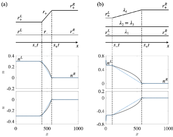
Figure 3: Riemann invariant configurations in the upper panels corresponding to theoretical (dotted) and numerical (solid) solutions. The vertical dashed lines correspond to $x_{\pm}=s_{\pm}(t-\bar{t})$, where $\bar{t}=30$ is the time delay introduced to account for the piston acceleration time. (a) RW solution with $u_{0}=-0.3$, satisfying the subsonic condition $|u_{0}|<\frac{1}{\sqrt{3}}$; (b) soliton|RW solution with $u_{0}=-0.7$, satisfying the supersonic condition $\frac{1}{\sqrt{3}}<|u_{0}|<1$

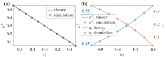
Figure 4: Theory and simulation results of the left constant state density $n^{L}$ for subsonic $|u_{0}|<\frac{1}{\sqrt{3}}$ (a) and supersonic $\frac{1}{\sqrt{3}}<|u_{0}|<1$ (b). The soliton amplitude $a$ is also shown in (b).

V.2 Supersonic Regime: $\mathbf{S}^{+}$|RW

When the piston velocity is supersonic with $u_{0}^{2}>\frac{1}{3}$, a contact soliton develops at the piston boundary smoothly connected to a RW via an intermediate constant state. The Riemann invariant configuration of the solution is shown in the top panel of Fig. 3(b). The soliton is represented by the Riemann invariants $\lambda_{2}=\lambda_{3}$.

This soliton is theoretically determined by (37)-(39) for a bright soliton. It is verified that when the piston is moving at the sonic speed $u_{0}=u_{\mathrm{cr}}=\pm\frac{1}{\sqrt{3}}$, the soliton does not exist, i.e. $a=0$. Therefore, the soliton at the piston boundary only emerges in the supersonic regime. A representative supersonic solution is shown in the bottom panel of Fig. 3(b), exhibiting good agreement with the numerical simulation. Across the supersonic domain, theoretical predictions of $n^{L}$ and $a$ of the soliton demonstrate excellent agreement with simulation results, shown in Fig. 4(b). Herein we have confirmed our assumptions proposed in Sec. IV on the characterization of the solitonic supersonic solutions. In addition, our analysis found that no vacuum state, where $|n|=1$ occurs. The largest magnitude of $n$ is reached at the peak (crest) of the elevation (depression) soliton at the piston boundary and this magnitude is always less than 1 for $\frac{1}{3}<u_{0}^{2}<1$.

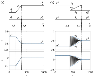
Figure 5: Riemann invariant configurations and the corresponding theoretical (dotted) and numerical (solid) solutions. The vertical dashed lines correspond to $x_{\pm}=s_{\pm}(t-\bar{t})$, where $\bar{t}=30$ is the time delay introduced to account for the piston acceleration time. (a) Sector I: $\mathrm{RW}$ with $u_{0}=-0.1$ and $h_{0}=0.8$. (b) Sector II: $\mathrm{DSW}^{+}$ with $u_{0}=0.2$ and $h_{0}=0.8$, the dotted curve is the theoretical DSW envelope.

VI Nonzero Applied Field, Subsonic Regime

In this section, we present subsonic solutions with nonzero applied field. The solution map is the white region of the phase diagram Fig. 2, including sectors I-IV. We consider each sector in turn.

VI.1 Sector I: RW

In sector I, the system satisfies the convexity condition (30) and yields simple wave solutions. Again, the solution is an expansive RW satisfying $r_{-}=r_{-}^{R}$, $r_{+}=r_{+}(\xi)$, and $v_{+}(r_{-},r_{+})=\xi=x/\left(t-\bar{t}\right)$. An example Riemann invariant configuration and solution in sector I is shown in Fig. 5(a). Good agreement between theory and simulation is demonstrated.

The admissibility condition (32) has been verified across sector I. The sonic condition is determined by $v_{+}=0$, yielding the boundary between sector I and V. Again, the sonic condition coincides with the admissibility threshold, indicating that only subsonic solutions are admissible in sector I. On the boundary between sector I and II which is the $h_{0}$-axis, there are no induced dynamics because $u_{0}=0$. Furthermore, no vacuum state is present in sector I since the largest magnitude of $n$ is at the piston boundary where the piston velocity is restricted to $|u_{0}|<1$.

VI.2 Sector II: $\mathbf{DSW}^{+}$

Sector II is to the left of the convexity curve (dotted black curve) in the phase diagram Fig. 2, so the system is convex, yielding simple wave solutions. Furthermore, $v_{+}(r_{-}^{R},r_{+}^{L})>v_{+}(r_{-}^{R},r_{+}^{R})$ leads to compressive DSW solutions that satisfy $\lambda_{3}=\lambda_{3}(\xi)$, $v_{3}(r_{-}^{R},r_{+}^{R},\lambda_{3},r_{+}^{L})=\xi=x/\left(t-\bar{t}\right)$. The DSW solutions satisfy the admissibility condition  (32). An example Riemann invariant configuration and solution in sector II is shown in Fig. 5(b). Near the DSW’s harmonic edge, the numerical simulation and the predicted envelope amplitude deviate somewhat. This is a common feature of the asymptotic (large $t$) behavior of DSWs [17]. Fig. 6 shows that, despite the piston acceleration period, the theoretically predicted trajectory of the DSW’s soliton edge differs from the simulation result by a constant time shift.

The DSW solution exhibits vacuum in the pink-shaded region in the phase diagram Fig. 2. The vacuum state is first reached when the maximum of the trailing edge soliton density $n=n_{4}$ reaches 1. We evaluate $n_{4}$ in the soliton limit, which is a function of the Riemann invariants, to determine this threshold (see Appendix). As time progresses, the vacuum point will move inside the oscillatory structure [17]. Example DSWs with vacuum will be shown in Fig. 8. We point out that the vacuum threshold determination is the same across all subsonic sectors whose solution contains a DSW structure, despite the convexity of the system.

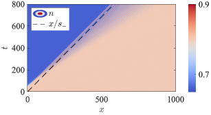
Figure 6: Space-time contour plot of a $\mathrm{DSW}^{+}$ solution in sector II with $u_{0}=0.2$, $h_{0}=0.8$. The black solid line is the predicted trailing edge soliton location for an ideal piston with instantaneous acceleration.

VI.3 Sector III: $\mathbf{DSW}^{+}\mathbf{CDSW}^{+}$

Sector III is to the right of the convexity curve (dotted black curve) in the phase diagram Fig. 2, so the solution breaks the convexity condition (30), manifested as the coalescence of two Riemann invariants $\lambda_{3}=\lambda_{4}$ and Whitham velocities $v_{3}=v_{4}$. The Riemann invariant configuration and an example solution are shown in Fig. 7(a), satisfying $r_{-}=r_{-}^{R}$, $\lambda_{3}=\lambda_{3}(\xi)$, and $v_{3}(r_{-}^{R},r_{+}^{R},\lambda_{3},r_{+}^{L})=\xi=x/\left(t-\bar{t}\right)$. The spin injection $u_{0}$ satisfies (40), leading to a compressive $\mathrm{DSW}^{+}\mathrm{CDSW}^{+}$ composite wave where $r_{+}^{L}>r_{+}^{R}$ gives the DSW portion and the coalescence of Riemann invariants $\lambda_{3}=\lambda_{4}$ gives the CDSW portion.

A CDSW is a degenerate DSW solution whose soliton limit is an algebraically decaying soliton where three Riemann invariants, $\lambda_{2}$, $\lambda_{3}$, and $\lambda_{4}$, coincide. The algebraic soliton travels at the speed of a dispersionless (long-wave) characteristic velocity, mimicking a contact discontinuity in viscous hydrodynamics. It is observed numerically that CDSWs generally require a longer time than DSWs to develop. Therefore, a larger discrepancy between the simulated CDSW portion and the analytical wave envelope is observed compared to the DSW portion. The admissibility of the composite wave solution in sector III, $0<s_{-}^{\mathrm{(1)}}<s_{-}^{\mathrm{(2)}}<s_{+}$, has been confirmed. The region where a vacuum state is present in the solution is shaded in pink in Fig. 2 and a typical solution is shown in Fig. 8(c).

VI.4 Sector IV: $\mathbf{RW}\,\mathbf{CDSW}^{+}$

Before moving on to sector IV, we discuss the solution on the boundary between sector III and IV, where $r_{+}^{L}=r_{+}^{R}$ as shown in the Riemann invariant configuration in Fig. 7(b). The system is nonconvex and the solution is a single $\mathrm{CDSW}^{+}$ because $\lambda_{3}=\lambda_{4}$ across the shock.

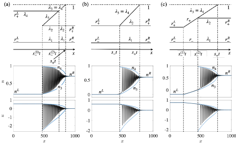
Figure 7: Riemann invariant configurations and example solutions when $h_{0}\neq 0$ for (a) Sector III: $\mathrm{DSW}^{+}\mathrm{CDSW}^{+}$ with $u_{0}=0.55$ and $h_{0}=0.7$; (b) Boundary of sectors III and IV: $\mathrm{CDSW}^{+}$ with $u_{0}=0.6$ and $h_{0}=0.6$. (c) Sector IV: $\mathrm{RW\,CDSW}^{+}$ with $u_{0}=0.73$ and $h_{0}=0.6$; The vertical dashed lines separate different components of the composite wave solutions based on predicted edge velocities. The dotted curves are the predicted envelopes of the DSW structure in the solution. In (b), the dotted curve also predicts the dispersionless RW portion of the solution. All modulation solutions include the time delay $\bar{t}=30$ to account for the piston acceleration time.

Sector IV is to the right of the convexity threshold (dotted black curve, Eq. (41)) in Fig. 2, so the system is nonconvex. During piston acceleration, compressive dynamics are induced, then followed by expansive dynamics. Thus, the solution is a $\mathrm{RW}\,\mathrm{CDSW}^{+}$ composite wave that satisfies $r_{-}=r_{-}^{R}$, $v_{3}(r_{-}^{R},r_{+}^{R},\lambda_{3},\lambda_{3})=\xi=x/\left(t-\bar{t}\right)$, and $\lambda_{4}=\lambda_{3}$. The Riemann invariant configuration and an example solution are shown in Fig. 7(c). The admissibility (32) of the solutions have been verified in the sector with the threshold $s_{-}^{(1)}=0$ coinciding with the sonic condition $v_{+}=0$ and Eq. (35). The vacuum region, shaded in pink in Fig. 2, is determined by evaluating the wave envelope $n_{4}$ in the algebraic soliton limit. The onset of vacuum is found to be independent of $u_{0}$ in this case and happens at $h_{0}=1/\sqrt{2}$. Representative solutions containing a vacuum point are shown in Fig. 8(c), (d).

In the example solutions shown in Fig. 7(b), (c), we observe that there is a smooth tail at the algebraic soliton limit of the CDSW when it connects to the dispersionless portion of the solution. This phenomenon is most evidently shown in Fig. 7(b) with a single CDSW. This behavior does not occur in DSWs where the exponential soliton edge terminates directly at the dispersionless edge state (see the bottom panels of Figs. 5(b) and 7(a)). This phenomenon serves as a distinguishing feature to identify the soliton edge of a CDSW.

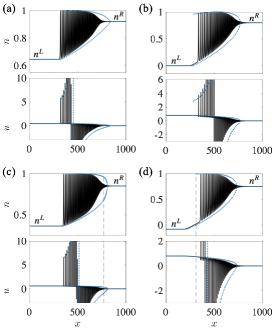
Figure 8: Example solutions with vacuum states when $h_{0}\neq 0$. (a) Sector II: $\mathrm{DSW}^{+}$ with $u_{0}=0.45$ and $h_{0}=0.92$; (b) Border of sectors II and III: $\mathrm{CDSW}^{+}$ with $u_{0}=0.8$ and $h_{0}=0.8$; (c) Sector III: $\mathrm{DSW}^{+}\mathrm{CDSW}^{+}$ with $u_{0}=0.6$ and $h_{0}=0.85$; (d) Sector IV: $\mathrm{RW}\,\mathrm{CDSW}^{+}$ with $u_{0}=0.8$ and $h_{0}=0.75$. The dotted curves are the predicted envelopes of the DSW structure. In (d), the dotted curve includes the predicted dispersionless RW portion in the solution. The vertical dashed lines separate different components in composite modulation solutions. The modulation solutions includes the time delay $\bar{t}=30$ to account for the piston acceleration time.

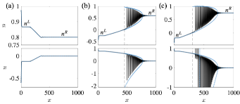
Figure 9: Supersonic solutions when $h_{0}\neq 0$. (a) Sector V: $\mathrm{S}^{+}|\mathrm{RW}$ with $u_{0}=-0.6$ and $h_{0}=0.8$; (b) Sector VI: $\mathrm{S}^{-}|\mathrm{RW}\,\mathrm{CDSW}^{+}$ with $u_{0}=0.92$ and $h_{0}=0.6$; (c) Sector VI: $\mathrm{S}^{-}|\mathrm{RW}\,\mathrm{CDSW}^{+}$ with a vacuum point, $u_{0}=0.96$ and $h_{0}=0.75$. The dotted curves trace the predicted piston edge soliton, the dispersionless portion of the solution, and the envelope of the DSW-type portion of the solution. The vertical dashed lines divide the different components in a composite wave based on the predicted edge velocities. The time delay $\bar{t}=30$ is used in theoretical plotting to account for the piston acceleration time.

VII Nonzero Applied Field, Supersonic Regime

Sectors V and VI satisfy the supersonic condition (35) in which $v_{-}<v_{+}<0$ and a contact soliton is developed at the piston boundary. Sector VII also satisfies the supersonic condition where $0<v_{-}<v_{+}$ and a PDSW emanates from the piston boundary.

VII.1 Sector V: $\mathbf{S}^{+}|\mathbf{RW}$

The contact soliton is uniquely determined by  (37)– (39). With the determined soliton far-field $(n^{L},u^{L})=(\bar{n},\bar{u})$, the modulation solution is an expansive RW, satisfying (31) and $r_{+}=r_{+}(\xi)$ where $v_{+}(r_{-},r_{+})=\xi=x/\left(t-\bar{t}\right)$. The admissibility condition (32) is satisfied. Similar to the zero field supersonic solution, no vacuum point is attained. A representative solution is shown in Fig. 9(a) with quantitative agreement between the theoretical prediction and the numerical simulation.

VII.2 Sector VI: $\mathbf{S}^{-}|\mathbf{RW}\,\mathbf{CDSW}^{+}$

The depression contact soliton is uniquely determined by (37)–(39) with far-field $(n^{L},u^{L})=(\bar{n},\bar{u})$ breaking the convexity condition (30), leading to a $\mathrm{RW}\,\mathrm{CDSW}^{+}$ composite wave satisfying $r_{-}=r_{-}^{R}$, $v_{3}=(r_{-}^{R},r_{+}^{R},\lambda_{3},\lambda_{3})=\xi=x/\left(t-\bar{t}\right)$, and $\lambda_{4}=\lambda_{3}$. A representative solution is shown in Fig. 9(b). Same as in sector IV, the onset of vacuum, when the algebraic soliton of the CDSW portion reaches 1, is independent of $u_{0}$ and happens at $h_{0}=1/\sqrt{2}$. This thresh The pink-shaded region in Fig. 2 indicates a vacuum state is present in the solution. A vacuum solution from this sector is shown in Fig. 9(c).

VII.3 Sector VII: PDSW⁺|DSW⁺

The supersonic condition $|u_{0}|>u_{\mathrm{cr}}(n^{L})$ in sector VII is $0<v_{-}<v_{+}$. This positive velocity configuration is different from all other supersonic sectors with negative dispersionless velocities. It gives rise to a PDSW [39] at the piston edge. For this sector, we focus on the qualitative identification of the solution features with the support of simulations. As we observed numerically (see Fig. 10(a) for example), the PDSW is led by a soliton at its right edge and terminates on the left at the piston boundary without reaching the small amplitude limit. The intermediate state connecting the PDSW and a DSW-type wave demonstrates slow oscillations that possibly is not a constant plateau and requires additional analysis. Without the PDSW far-field determined, we are unable to determine the modulation solution. Note that a vacuum point is present inside the solution, consistent with our prediction in Fig. 2.

We have numerically confirmed that along the sonic curve bounding the subsonic sector II, where the system remains convex, there is no PDSW emerging from the piston boundary. However, within the nonconvex subsonic sector III when near the sonic curve at the sector VII boundary, we numerically observed that a PDSW develops at the piston boundary as shown in Fig. 10(b). Consequently, the predicted sonic boundary between sectors III and III does not precisely explain this phase change. We have not been able to quantitatively identify the threshold for the occurrence of this phase transition using modulation theory. However, all simulations that we have performed in sector VII exhibit this PDSW structure.

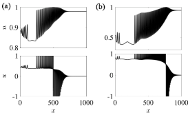
Figure 10: (a) $\mathrm{PDSW}|\mathrm{DSW}^{+}$ solution in sector VII with $u_{0}=0.45$ and $h_{0}=0.98$. (b) Supercritical solution in sector III with $u_{0}=0.8$ and $h_{0}=0.95$.

VIII Conclusion

Using the dispersive hydrodynamic framework, we have analytically classified the piston-like dynamics of a dissipationless easy-plane ferromagnetic channel subject to spin injection at one channel boundary. This framework enables the analytical description of noncollinear magnetic textures beyond the small-amplitude, weakly nonlinear regime.

Two properties of the system is fundamental to our analysis. First, the piston analogy naturally leads to the investigation of magnetic sub- to supersonic conditions, corresponding to distinct piston boundary behavior: either a constant hydrodynamic flow in the subsonic case, or a soliton or a non-stationary partial DSW (PDSW) both in the supersonic case. We provided quantitative characterization of the solutions using the modulation theory and qualitative identification of the PDSW solutions, where a sharp threshold for this behavior is yet to be determined.

Second, the modulation equations exhibit nonconvexity where the modulation velocities coalesce. Adopting the method developed in [30], a non-classical dispersive shock wave solution, a contact DSW (CDSW), is predicted when the system exhibits nonconvexity as a single wave or one component of a composite wave. A distinguishing feature is a short, smooth ramp at the algebraic soliton edge of a CDSW where the soliton connects to a dispersionless (non-oscillatory) portion of the solution.

While our analysis was developed for conservative spin dynamics applicable over short enough time scales, it has intriguing implications for longer times wherein magnetic damping leads to relaxation of the dynamics to a steady configuration. First, rarefaction waves expand in time with negligible oscillations. This implies that such a solution minimizes the excitation of spin waves in the system. On the contrary, spin shocks exhibit pronounced oscillations that can reflect many times in the channel before being quenched by magnetic damping. While this can be seen as a disadvantage, it is also important to note that the spin waves excited by a spin shock are launched within a specific spectral band that is determined by the transition between the left and right states [40], opening opportunities for controllable transport of angular momentum by means of pulsed injection. Second, we find that a stationary soliton established in the conservative regime can remain after stabilization via damping, resulting in the contact soliton-dissipative exchange flow [10]. Third, numerical simulations in [12] show that it is also possible to excite propagating soliton trains that persist, oscillating back and forth in the channel, even in the presence of damping. In additional simulataions, we observe here that such solitons are excited precisely when the originating spin shock contains a CDSW. These are examples of situations where the transient dynamics impact the transport characteristics of the dissipative exchange flow in equilibrium.

The dispersive hydrodynamic interpretation of ferromagnetic dynamics allows one to adopt a large pool of analytical tools that are traditionally used for classical fluids, which provides new perspectives on the study and understanding of spin dynamics. The dynamical problem studied here has a problem setup that is designed to be experimentally accessible and we expect our methodology to aid the experimental realization of superfluid-like spin transport in the form of nonuniform magnetic textures.

IX Acknowledgment

M. Hu thanks T. Congy for the helpful discussions. All authors acknowledge support from the U.S. Department of Energy, Office of Science, grant DE-SC0018237. M. Hoefer acknowledges partial support from National Science Foundation DMS-1816934 and M. Hu acknowledges support from the National Institute of Standards and Technology Professional Research Experience Program.

*

Appendix A Appendix: Determination of the Physical Wave Pattern Given Riemann Invariants

In this appendix, we present additional information on the characterization of periodic traveling wave solutions to the LL equation (1). The LL-Whitham equations in terms of the Riemann invariants $\mathbf{\lambda}=(\lambda_{1},\lambda_{2},\lambda_{3},\lambda_{4})$ have been given in (23). The family of traveling waves dynamics satisfy Eq. (8). The quartic polynomial $R(n)$ can be written in terms of four roots $\{n_{i}\}_{i=1}^{4}$. It can also be expressed in terms of the Riemann invariants $\bm{\lambda}$ [30] where

$$\begin{split}R(n)=&n^{4}+\frac{s_{1}+s_{3}}{f_{1}}n^{3}+s_{2}n^{2}+(f_{1}s_{1}-\frac{s_{1}+s_{3}}{f_{1}})n\\ &+\frac{1}{4}(s^{2}_{1}-4-4s_{2}+4f_{1}^{2}),\end{split}$$ (43)

$$\begin{split}&s_{1}=\displaystyle\sum_{i}^{4}\lambda_{i},\ s_{2}=\displaystyle\sum_{i<j}^{4}\lambda_{i}\lambda_{j},\ s_{3}=\displaystyle\sum_{i<j<k}^{4}\lambda_{i}\lambda_{j}\lambda_{k},\\ &s_{4}=\lambda_{1}\lambda_{2}\lambda_{3}\lambda_{4},\end{split}$$ (44)

$$\lambda_{i}^{\prime}=\sqrt{1-\lambda_{i}^{2}},\ s_{4}^{\prime}=\Pi_{i}^{4}\lambda_{i}^{\prime}.$$ (45)

For a given set of Riemann invariants $\bm{\lambda}$, there are four possible physical wave patterns corresponding to four possible choices of $f_{1}$:

$$f_{1} =\pm\sqrt{(1+s_{2}+s_{4}+s_{4}^{\prime})/2},$$ (46a)

$$\mathrm{or\ }f_{1} =\pm\text{sgn}(s_{1}+s_{3})\sqrt{(1+s_{2}+s_{4}-s_{4}^{\prime})/2},$$ (46b)

This 4-valued mapping of Riemann invariants to traveling wave profiles implies that the LL-Whitham modulation system is nonconvex. Later, we denote $f_{1a}$ as $f_{1}$ taking the positive expression in (46a) and $f_{1b}$ as $f_{1}$ taking the positive expression in (46b). The fluid velocity can be computed from the density as

$$u(\xi)=-\frac{f_{1}+\frac{s_{1}}{2}n}{1-n^{2}}.$$ (47)

The multi-valued mapping from the Riemann invariants to the roots of the potential function are [30]:

$$n_{1} =-\frac{1}{2f_{1}}\frac{(\lambda_{3}-\lambda_{2})\tilde{s}_{1}+(\lambda_{3}-\lambda_{1})\tilde{s}_{2}-(\lambda_{2}-\lambda_{1})\tilde{s}_{3}}{(\lambda_{3}-\lambda_{2})\lambda_{1}^{\prime}+(\lambda_{3}-\lambda_{1})\lambda_{2}^{\prime}-(\lambda_{2}-\lambda_{1})\lambda_{3}^{\prime}},$$ (48)

$$n_{2} =-\frac{1}{2f_{1}}\frac{(\lambda_{3}-\lambda_{2})\tilde{s}_{1}+(\lambda_{3}-\lambda_{1})\tilde{s}_{2}+(\lambda_{2}-\lambda_{1})\tilde{s}_{3}}{(\lambda_{3}-\lambda_{2})\lambda_{1}^{\prime}+(\lambda_{3}-\lambda_{1})\lambda_{2}^{\prime}+(\lambda_{2}-\lambda_{1})\lambda_{3}^{\prime}},$$

$$n_{3} =-\frac{1}{2f_{1}}\frac{(\lambda_{3}-\lambda_{2})\tilde{s}_{1}-(\lambda_{3}-\lambda_{1})\tilde{s}_{2}-(\lambda_{2}-\lambda_{1})\tilde{s}_{3}}{(\lambda_{3}-\lambda_{2})\lambda_{1}^{\prime}-(\lambda_{3}-\lambda_{1})\lambda_{2}^{\prime}-(\lambda_{2}-\lambda_{1})\lambda_{3}^{\prime}},$$

$$n_{4} =-\frac{1}{2f_{1}}\frac{(\lambda_{3}-\lambda_{2})\tilde{s}_{1}-(\lambda_{3}-\lambda_{1})\tilde{s}_{2}+(\lambda_{2}-\lambda_{1})\tilde{s}_{3}}{(\lambda_{3}-\lambda_{2})\lambda_{1}^{\prime}-(\lambda_{3}-\lambda_{1})\lambda_{2}^{\prime}+(\lambda_{2}-\lambda_{1})\lambda_{3}^{\prime}},$$

where $\tilde{s}_{i}=(s_{1}-\lambda_{i})\lambda_{i}^{\prime}+s_{4}\frac{\lambda_{i}^{\prime}}{\lambda_{i}}\mp s_{4}^{\prime}\frac{\lambda_{i}}{\lambda_{i}^{\prime}}$. The upper sign in $\tilde{s}_{i}$ is for $f_{1a}$ given by (46a) and the lower sign is for $f_{1b}$ given by (46b). The other two cases when $f_{1}<0$ leads to reordering of the expressions of $n_{i}$’s, which is $n_{i}\leftarrow n_{5-i}$, $i=1,2,3,4$.

Depending on which triangle, divided by the diagonal and anti-diagonal of the square $[-1,1]\times[-1,1]$ the left constant state $(u^{L},n^{L})$ lies in, the choice of $f_{1}$ is shown in Fig. A1.

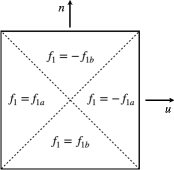
Figure A1: The choice of $f_{1}$ depending on the location of $(u^{L},n^{L})$.

References

- Iacocca and Hoefer [2019a] E. Iacocca and M. A. Hoefer, Perspectives on spin hydrodynamics in ferromagnetic materials, Physics Letters A 383, 125858 (2019a).
- Sonin [2020] E. B. Sonin, Superfluid spin transport in magnetically ordered solids (Review article), Low Temperature Physics 46, 436 (2020).
- Halperin and Hohenberg [1969] B. Halperin and P. Hohenberg, Hydrodynamic theory of spin waves, Physical Review 188, 898 (1969).
- König et al. [2001] J. König, M. C. Bønsager, and A. H. MacDonald, Dissipationless spin transport in thin film ferromagnets, Physical Review Letters 87, 187202 (2001).
- Sonin [2010] E. Sonin, Spin currents and spin superfluidity, Advances in Physics 59, 181 (2010).
- Takei and Tserkovnyak [2014] S. Takei and Y. Tserkovnyak, Superfluid spin transport through easy-plane ferromagnetic insulators, Physical review letters 112, 227201 (2014).
- Chen et al. [2014] H. Chen, A. D. Kent, A. H. MacDonald, and I. Sodemann, Nonlocal transport mediated by spin supercurrents, Physical Review B 90, 220401 (2014).
- Iacocca et al. [2017a] E. Iacocca, T. Silva, and M. A. Hoefer, Breaking of Galilean Invariance in the Hydrodynamic Formulation of Ferromagnetic Thin Films, Physical Review Letters 118, 10.1103/PhysRevLett.118.017203 (2017a).
- Iacocca et al. [2017b] E. Iacocca, T. J. Silva, and M. A. Hoefer, Symmetry-broken dissipative exchange flows in thin-film ferromagnets with in-plane anisotropy, Physical Review B 96, 134434 (2017b).
- Iacocca and Hoefer [2019b] E. Iacocca and M. A. Hoefer, Hydrodynamic description of long-distance spin transport through noncollinear magnetization states: Role of dispersion, nonlinearity, and damping, Physical Review B 99, 10.1103/PhysRevB.99.184402 (2019b).
- Evers and Nowak [2020] M. Evers and U. Nowak, Transport properties of spin superfluids: Comparing easy-plane ferromagnets and antiferromagnets, Physical Review B 101, 184415 (2020).
- Hu et al. [2021] M. Hu, E. Iacocca, and M. A. Hoefer, Spin-injection-generated shock waves and solitons in a ferromagnetic thin film, IEEE Transactions on Magnetics (2021).
- Smith et al. [2021] D. A. Smith, S. Takei, B. Brann, L. Compton, F. Ramos-Diaz, M. Simmers, and S. Emori, Diffusive and fluid-like motion of homochiral domain walls in easy-plane magnetic strips, arXiv preprint arXiv:2107.07025 (2021).
- Stepanov et al. [2018] P. Stepanov, S. Che, D. Shcherbakov, J. Yang, R. Chen, K. Thilahar, G. Voigt, M. W. Bockrath, D. Smirnov, K. Watanabe, et al., Long-distance spin transport through a graphene quantum hall antiferromagnet, Nature Physics 14, 907 (2018).
- Schneider et al. [2018] T. Schneider, D. Hill, A. Kakay, K. Lenz, J. Lindner, J. Fassbender, P. Upadhyaya, Y. Liu, K. Wang, Y. Tserkovnyak, et al., Self-stabilizing spin superfluid, arXiv preprint arXiv:1811.09369 (2018).
- Yuan et al. [2018] W. Yuan, Q. Zhu, T. Su, Y. Yao, W. Xing, Y. Chen, Y. Ma, X. Lin, J. Shi, R. Shindou, et al., Experimental signatures of spin superfluid ground state in canted antiferromagnet cr2o3 via nonlocal spin transport, Science advances 4, eaat1098 (2018).
- El and Hoefer [2016] G. El and M. Hoefer, Dispersive shock waves and modulation theory, Physica D: Nonlinear Phenomena 333, 11 (2016).
- Iacocca and Hoefer [2017] E. Iacocca and M. A. Hoefer, Vortex-antivortex proliferation from an obstacle in thin film ferromagnets, Physical Review B 95, 134409 (2017).
- Iacocca [2020] E. Iacocca, Controllable vortex shedding from dissipative exchange flows in ferromagnetic channels, Physical Review B 102, 224403 (2020).
- Janantha et al. [2017] P. P. Janantha, P. Sprenger, M. A. Hoefer, and M. Wu, Observation of self-cavitating envelope dispersive shock waves in yttrium iron garnet thin films, Physical Review Letters 119, 024101 (2017).
- Hoefer et al. [2006] M. A. Hoefer, M. J. Ablowitz, I. Coddington, E. A. Cornell, P. Engels, and V. Schweikhard, Dispersive and classical shock waves in Bose-Einstein condensates and gas dynamics, Phys. Rev. A 74, 023623 (2006).
- Bienaimé et al. [2021] T. Bienaimé, M. Isoard, Q. Fontaine, A. Bramati, A. Kamchatnov, Q. Glorieux, and N. Pavloff, Quantitative Analysis of Shock Wave Dynamics in a Fluid of Light, Physical Review Letters 126, 183901 (2021).
- Xu et al. [2017] G. Xu, M. Conforti, A. Kudlinski, A. Mussot, and S. Trillo, Dispersive Dam-Break Flow of a Photon Fluid, Physical Review Letters 118, 254101 (2017).
- Trillo et al. [2016] S. Trillo, M. Klein, G. Clauss, and M. Onorato, Observation of dispersive shock waves developing from initial depressions in shallow water, Physica D 333, 276 (2016).
- Maiden et al. [2016] M. D. Maiden, N. K. Lowman, D. V. Anderson, M. E. Schubert, and M. A. Hoefer, Observation of Dispersive Shock Waves, Solitons, and Their Interactions in Viscous Fluid Conduits, Physical Review Letters 116, 174501 (2016).
- Liepmann and Roshko [1957] H. W. Liepmann and A. Roshko, Elements of Gasdynamics (Wiley, New York, 1957).
- Whitham [2011] G. B. Whitham, Linear and nonlinear waves, Vol. 42 (John Wiley & Sons, 2011).
- Kamchatnov [2000] A. M. Kamchatnov, Nonlinear periodic waves and their modulations: an introductory course (World Scientific, 2000).
- Riemann [1860] B. Riemann, Über die Fortpflanzung ebener Luftwellen von endlicher Schwingungsweite, Abh. d. Königl. Ges. d. Wiss. zu Göttingen 8, 43 (1860).
- Ivanov et al. [2017] S. K. Ivanov, A. M. Kamchatnov, T. Congy, and N. Pavloff, Solution of the Riemann problem for polarization waves in a two-component Bose-Einstein condensate, Physical Review E 96, 10.1103/PhysRevE.96.062202 (2017).
- Hoefer et al. [2008] M. A. Hoefer, M. J. Ablowitz, and P. Engels, Piston Dispersive Shock Wave Problem, Physical Review Letters 100, 10.1103/PhysRevLett.100.084504 (2008).
- Kamchatnov and Korneev [2010] A. M. Kamchatnov and S. V. Korneev, Flow of a Bose-Einstein condensate in a quasi-one-dimensional channel under the action of a piston, Journal of Experimental and Theoretical Physics 110, 170 (2010).
- Mossman et al. [2018] M. E. Mossman, M. A. Hoefer, K. Julien, P. G. Kevrekidis, and P. Engels, Dissipative shock waves generated by a quantum-mechanical piston, Nature Communications 9, 4665 (2018).
- Bendahmane et al. [2020] A. Bendahmane, G. Xu, M. Conforti, A. Kudlinski, A. Mussot, and S. Trillo, Phase transitions of photon fluid flows driven by a virtual all-optical piston, arXiv preprint arXiv:2007.16060 (2020).
- El et al. [2017] G. El, M. Hoefer, and M. Shearer, Dispersive and diffusive-dispersive shock waves for nonconvex conservation laws, SIAM Review 59, 3 (2017).
- Byrd and Friedman [1954] P. F. Byrd and M. D. Friedman, Handbook of Elliptic Integrals for Engineers and Physicists (Springer-Verlag, 1954).
- Lax [1973] P. D. Lax, Hyperbolic Systems of Conservation Laws and the Mathematical Theory of Shock Waves (SIAM, 1973).
- Courant and Friedrichs [1948] R. Courant and K. O. Friedrichs, Supersonic Flow and Shock Waves (Springer-Verlag, 1948).
- Marchant and Smyth [1991] T. Marchant and N. Smyth, Initial-boundary value problems for the korteweg-de vries equation, IMA journal of applied mathematics 47, 247 (1991).
- Conforti et al. [2014] M. Conforti, F. Baronio, and S. Trillo, Resonant radiation shed by dispersive shock waves, Phys. Rev. A 89, 013807 (2014).
- Madami et al. [2011] M. Madami, S. Bonetti, G. Consolo, S. Tacchi, G. Carlotti, G. Gubbiotti, F. Mancoff, M. A. Yar, and J. Åkerman, Direct observation of a propagating spin wave induced by spin-transfer torque, Nature nanotechnology 6, 635 (2011).
- Cornelissen et al. [2015] L. Cornelissen, J. Liu, R. Duine, J. B. Youssef, and B. Van Wees, Long-distance transport of magnon spin information in a magnetic insulator at room temperature, Nature Physics 11, 1022 (2015).
- Wesenberg et al. [2017] D. Wesenberg, T. Liu, D. Balzar, M. Wu, and B. L. Zink, Long-distance spin transport in a disordered magnetic insulator, Nature Physics 13, 987 (2017).
- Liu et al. [2018] C. Liu, J. Chen, T. Liu, F. Heimbach, H. Yu, Y. Xiao, J. Hu, M. Liu, H. Chang, T. Stueckler, et al., Long-distance propagation of short-wavelength spin waves, Nature communications 9, 1 (2018).
- Lebrun et al. [2018] R. Lebrun, A. Ross, S. Bender, A. Qaiumzadeh, L. Baldrati, J. Cramer, A. Brataas, R. Duine, and M. Kläui, Tunable long-distance spin transport in a crystalline antiferromagnetic iron oxide, Nature 561, 222 (2018).
- Sonin [2017] E. Sonin, Spin superfluidity and spin waves in yig films, Physical Review B 95, 144432 (2017).
- Sonin [2019] E. Sonin, Superfluid spin transport in ferro-and antiferromagnets, Physical Review B 99, 104423 (2019).
- Zhang et al. [2012] Y. Zhang, T.-H. Chuang, K. Zakeri, J. Kirschner, et al., Relaxation time of terahertz magnons excited at ferromagnetic surfaces, Physical review letters 109, 087203 (2012).
- Cornelissen et al. [2016] L. J. Cornelissen, K. J. Peters, G. E. Bauer, R. Duine, and B. J. van Wees, Magnon spin transport driven by the magnon chemical potential in a magnetic insulator, Physical Review B 94, 014412 (2016).
- Skarsvåg et al. [2015] H. Skarsvåg, C. Holmqvist, and A. Brataas, Spin superfluidity and long-range transport in thin-film ferromagnets, Physical review letters 115, 237201 (2015).
- Congy et al. [2016] T. Congy, A. Kamchatnov, and N. Pavloff, Dispersive hydrodynamics of nonlinear polarization waves in two-component Bose-Einstein condensates, SciPost Physics 1, 10.21468/SciPostPhys.1.1.006 (2016).
- Law et al. [2001] C. Law, C. Chan, P. Leung, and M.-C. Chu, Critical velocity in a binary mixture of moving bose condensates, Physical Review A 63, 063612 (2001).
- Qu et al. [2016] C. Qu, L. P. Pitaevskii, and S. Stringari, Magnetic Solitons in a Binary Bose-Einstein Condensate, Physical Review Letters 116, 10.1103/PhysRevLett.116.160402 (2016).
- Kamchatnov et al. [2014] A. M. Kamchatnov, Y. V. Kartashov, P.-E. Larre, and N. Pavloff, Nonlinear polarization waves in a two-component Bose-Einstein condensate, Physical Review A 89, 10.1103/PhysRevA.89.033618 (2014).
- Bendahmane et al. [2018] A. Bendahmane, G. Xu, M. Conforti, A. Kudlinski, A. Mussot, and S. Trillo, Optical fiber analogous of the piston shock problem, in Integrated Photonics Research, Silicon and Nanophotonics (Optical Society of America, 2018) pp. JTu6G–2.
- Whitham [1965] G. B. Whitham, Non-linear dispersive waves, Proceedings of the Royal Society of London. Series A. Mathematical and Physical Sciences 283, 238 (1965).
- Bookman [2015] L. D. Bookman, Approximate solitons of the landau-lifshitz equation, Ph. D. Thesis (2015).