Collective Autoscaling for Cloud Microservices
Abstract.
As cloud applications shift from monoliths to loosely coupled microservices, application developers must decide how many compute resources (e.g., number of replicated containers) to assign to each microservice within an application. This decision affects both (1) the dollar cost to the application developer and (2) the end-to-end latency perceived by the application user. Today, individual microservices are autoscaled independently by adding VMs whenever per-microservice CPU or memory utilization crosses a configurable threshold. However, an application user’s end-to-end latency consists of time spent on multiple microservices and each microservice might need a different number of VMs to achieve an overall end-to-end latency.
We present COLA, an autoscaler for microservice-based applications, which collectively allocates VMs to microservices with a global goal of minimizing dollar cost while keeping end-to-end application latency under a given target. Using 5 open-source applications, we compared COLA to several utilization and machine learning based autoscalers. We evaluate COLA across different compute settings on Google Kubernetes Engine (GKE) in which users manage compute resources, GKE standard, and a new mode of operation in which the cloud provider manages compute infrastructure, GKE Autopilot. COLA meets a desired median or tail latency target on 53 of 63 workloads where it provides a cost reduction of 19.3%, on average, over the next cheapest autoscaler. COLA is the most cost effective autoscaling policy for 48 of these 53 workloads. The cost savings from managing a cluster with COLA result in COLA paying for its training cost in a few days. On smaller applications, for which we can exhaustively search microservice configurations, we find that COLA is optimal for 90% of cases and near optimal otherwise.
1. Introduction
Cloud applications are increasingly built out of loosely coupled microservices communicating over RPCs(Netflix, [n.d.]; Twitter, [n.d.]; Uber, [n.d.]). Building applications out of microservices allow teams in large organizations to independently develop code with fewer concerns about programming language choice and code dependencies. This reduces friction in development.
However, this decomposition into microservices complicates autoscaling: the process of automatically allocating compute resources to a cloud application as its workload changes. Today, each microservice within an application is typically autoscaled independent of other microservices using a combination of two mechanisms: (1) horizontal pod autoscaling (HPA), which changes the number of replicas supporting a microservice and (2) cluster autoscaling, which changes the number of VMs to accommodate the change in the number of replicas induced by HPA.
This independent per-microservice autoscaling design is sub-optimal because it ignores the fact that each microservice operates in the broader context of a Web service application. In particular, while allocating additional VMs to a particular microservice does improve the response latency of RPCs served by this microservice, this improvement may have little impact on end-to-end latency of the application because of a much more sluggish microservice upstream or downstream.
Instead, we collectively autoscale all of an application’s microservices and decide how much to allocate each microservice, with a view towards a global objective. Effectively, we replace many distributed and independent autoscalers with one centralized autoscaler with global visibility.
To collectively autoscale a microservice-based application, we frame autoscaling of microservices as constrained optimization. The constraint is meeting an end-to-end mean/tail latency target. The optimization objective is minimizing dollar cost. Ideally, we would solve this optimization problem online as the workload and the microservices’ business logic change. But, finding the right number of VMs for each microservice takes time because it requires iteratively identifying and eliminating bottlenecked microservices until the end-to-end latency target is met. Running this iteration online can seriously disrupt the application’s user experience.
Instead, we propose COLA, an offline search process to find the right allocation of VMs to each microservice given some information on the workload that is expected during deployment.111This information doesn’t have to be perfect: COLA will interpolate between known workloads if possible and fall back to default autoscalers if not. COLA’s search process works as follows: for each workload, COLA applies the workload, identifies the most congested microservice (the microservice whose CPU utilization increases the most in response to the workload), determines the right allocation of VMs to this microservice using a bandit problem with a reward capturing the latency-vs.-cost tradeoff, then iterates this procedure with the next most-congested microservice until the latency target is met.
Effectively, from the perspective of an application developer, COLA performs profile-guided optimization (Lattner, 2002; Homescu et al., 2013) in the same spirit as a compiler that exploits knowledge of what program paths are more or less common to optimize generated code. Naively, this offline search process needs to explore all possible allocations of VMs to microservices, which blows up quickly. Hence, we develop optimizations to efficiently search this space and save both time and cost.
| Application | Microservices | Cost Reduction |
|---|---|---|
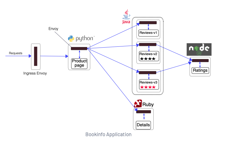
| Simple Web Server (Istio, [n.d.]b) | 1 | 13.95% |
| Book Info (Istio, [n.d.]a) | 4 | 18.01% |
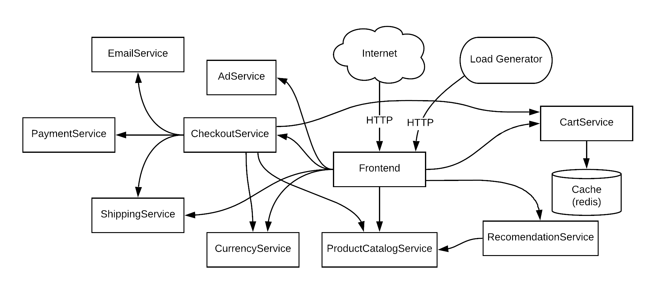
| Online Boutique (Weaveworks, [n.d.]) | 11 | 33.11% |
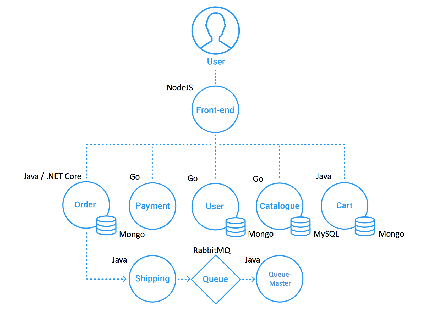
| Sock Shop (Google, [n.d.]c) | 14 | 1.34% |
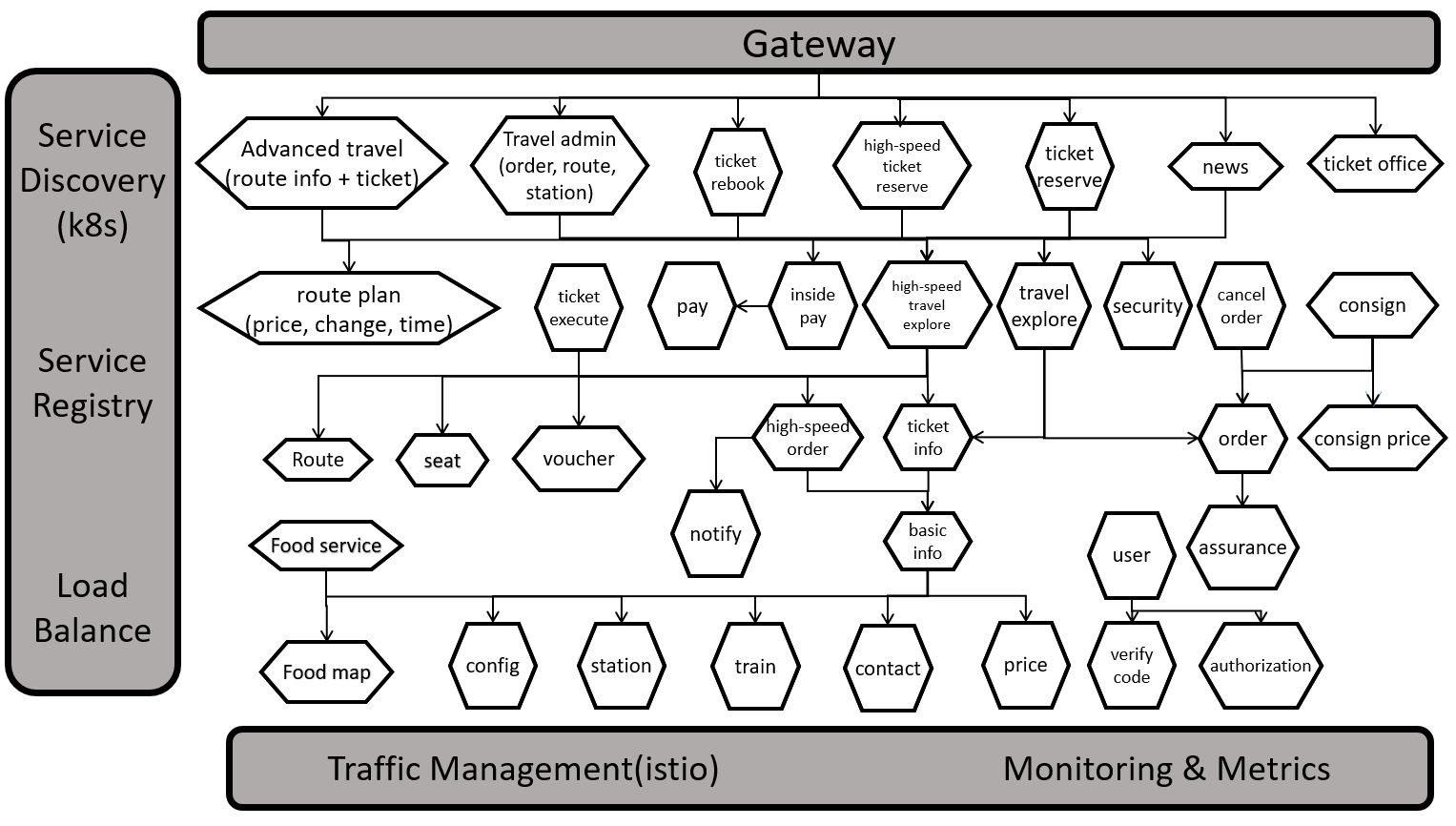
| Train Ticket (Zhou et al., 2018) | 64 | 26.25% |
We summarize our evaluations of COLA below:
-
(1)
Across 5 open source applications including the largest available open source application in terms of number of microservices (Zhou et al., 2018), on the Google Kubernetes Engine (GKE) platform, COLA outperforms 5 baselines (2 based on Kubernetes’ autoscaler (Kubernetes, [n.d.]b) and 3 ML-based research autoscalers (Alipourfard et al., 2017; Venkataraman et al., 2016; Qiu et al., 2020) adapted from the literature) (Table 1). Across 53 of 63 workloads where COLA meets a desired latency target, COLA reduces cost of microservice deployment by 19.3% when compared to the next cheapest autoscaler across our 5 baselines. On the remaining 10 workloads, the lowest cost policy which meets the corresponding latency target costs 69.9% more than COLA. Further, we evaluate and find that COLA outperforms baselines on a set of different compute environments where we vary node size and cluster type. A full set of tabular results is provided in Appendix Tables 16-38.
-
(2)
We demonstrate that initial training costs for COLA are paid for by the cost savings of deployment in less than one day in some cases and within a week for most cases. Additionally, we find COLA can be incrementally retrained for new latency targets and workloads with small overhead.
-
(3)
Empirically, we find that COLA’s results are near-optimal: typically, all other allocations of VMs to microservices either require more total VMs than COLA or do not satisfy the latency target.
-
(4)
Theoretically, using simplified models of interconnected microservices, we provide a mathematical rationale for COLA’s training and inference procedures. We show why utilization is a sensible metric to determine which microservice is most congested and also why linearly interpolating COLA’s policies can generalize to unseen workloads.
2. Background
2.1. Kubernetes
When developing a microservice application, developers deploy each microservice on one or more containers. Kubernetes (Kubernetes, [n.d.]c) is a platform that orchestrates the deployment, scaling, and management of these containers. We review Kubernetes concepts and control plane actions to describe how containers are deployed and are allocated compute resources.
Kubernetes Concepts. A Kubernetes cluster is made up of a set of nodes. Each node is a physical or virtual machine. A master node is responsible for hosting an entry point for interacting with the cluster, managing cluster state and scheduling resources. Worker nodes run an agent, known as a kubelet, to communicate with this master node. They also run containers within an application. Within worker nodes, the master node deploys pods: the atomic element of deployment, replication, and scaling in Kubernetes. A pod is an encapsulation of one or more containerized applications (typically one) along with a shared context of storage and network resources. A pod also has associated CPU and memory limits, which restrict the amount of the node’s resources that the pod is allowed to use.
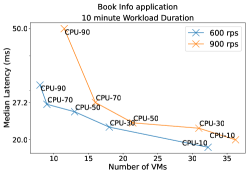
vs. Number of VMs for Book Info App
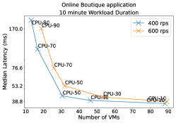
vs. Number of VMs for Online Boutique App
Autoscaling Mechanisms in Kubernetes. There are three primary mechanisms to automatically scale microservice application clusters managed by Kubernetes: Horizontal Pod Autoscaling (HPA), Vertical Pod Autoscaling (VPA) and Cluster Autoscaling (CA). HPA refers to automatically increasing or decreasing the number of replicas/pods of a pod deployment (in our case each deployment corresponds to one microservice), in response to changes in application or system metrics (i.e., CPU or memory utilization). VPA automatically increases the CPU or memory limits associated with one or more pods. VPA can increase or decrease either the minimum resource available for a pod (“CPU or Memory Request”) or the maximum resource available for a pod (“CPU or Memory Limit”). CA adds or removes additional nodes (physical or virtual machines) to a cluster. While HPA and VPA are provided by the Kubernetes system, CA is provided by the underlying infrastructure/cloud provider, e.g., Google Kubernetes Engine (GKE)(Google, [n.d.]b), Amazon Elastic Kubernetes Service (EKS) (Amazon, [n.d.]), and Microsoft’s Azure Kubernetes Service (AKS) (Microsoft, [n.d.]). CA in the cloud modifies the cluster size and adjusts the amount of resources rented from a cloud provider, directly affecting the dollar cost required to operate a cluster.
Autoscaling Policies in Kubernetes. We now describe the Kubernetes autoscaling policies that leverage the autoscaling mechanisms above. We focus on HPA as it is generally more aligned with facilitating cost efficient policies in latency sensitive applications for a few technical reasons. First, VPA reduces cluster cost less generally than HPA. Reducing cost with VPA relies on decreasing the size of underlying VMs which is a procedure not generally available across cloud providers. In the public cloud, it is in a cloud tenant’s interest to statically set their pod limits so that the pod can fully utilize the VM since tenants pay full price for a VM regardless of how well utilized it is. Further, when containers are scaled by increasing pod limits with VPA, they are restarted and potentially rescheduled to new VMs which meet their new limits. As a result availability and end-to-end latency can often be negatively impacted more than with a procedure such as HPA. As a result, managing a cluster without disruptions which is scaled with VPA can lead to provisioning compute resources for peak load. Since our aim is to find cost efficient autoscaling for latency sensitive services, we examine COLA in the context of HPA. The technical challenges in using VPA for our goal may contribute to HPA being used much more commonly than VPA; for instance, a recent survey of Datadog’s customers (Datadog, [n.d.]a) (who in aggregate deployed 1.5 billion containers) shows that roughly 40% of their customers have adopted HPA, while less than 1% use VPA.
Kubernetes HPA Autoscaling For HPA, Kubernetes natively offers utilization-based autoscalers which match the Autopilot (Rzadca et al., 2020) implementation. These autoscalers are implemented as a control loop with an update period (default of 15 seconds). At each period, the controller queries the resource utilization for the pods of each microservice as a percentage of the total resources requested by those pods. At any point in time, , the number of desired replicas is given by the following formula where is the current number of replicas, is the mean utilization and is the target utilization value: . Each microservice within an application is designated a target utilization value and scaled independently of others based on the above equation. The utilization here could refer to either CPU utilization or memory utilization.
2.2. Limitations of Kubernetes HPA
Utilization-based HPA is natively available in Kubernetes and simple to deploy. But, it suffers from key issues when trying to optimize an end-to-end latency target. We highlight these using controlled experiments.
Evaluation Setup. We evaluate 2 open source microservice applications on GKE (Google, [n.d.]b): Online Boutique (Google, [n.d.]c) and Book Info (Istio, [n.d.]a). For each application, we run 2 workloads; each workload has a different number of requests per second submitted to the application. For each workload, we examine the effects of using 5 different CPU utilization thresholds (10%, 30%, 50%, 70% and 90%) for a CPU utilization threshold HPA. For our evaluations, each replica requests all of the resources of one virtual machine. Consequently, the number of replicas equals the number of VMs a cloud customer would pay for. The results of the evaluation are shown in Figure 1.
HPA Shortcomings. We find that HPA utilization threshold choice dramatically effects the end-to-end latency and dollar cost of an application. For example, the Online Boutique application’s median latency ranges from 37 ms to 202 ms with 88 and 13 VMs rented respectively for the 400 request per second workload. The choice of utilization threshold in this case can lead to a 5.5 range in latency or a 6.8 range in cost. We also find that choosing the “best” policy, i.e., the utilization threshold which achieves a developer’s latency target at the lowest cost, is difficult because:
-
(1)
The best policy depends on the application. Given a latency target and/or cost objective there is no easy way to select a utilization threshold which meets the target without experimentation. From Figure 1 we can see that maintaining a lower utilization results in lower latency, but no closed-form mapping between these two quantities is available to a user. Further, as seen in Figure 1 for a fixed utilization threshold, end-to-end latencies are very different across Online Boutique and Book Info.
-
(2)
The best policy depends on the workload. Depending on the workload, the appropriate policy to meet a latency target changes. In Figure 1 we compare two workloads where one workload has 50% more requests per second than the other. As seen for Online Boutique in the center graph, a 50% CPU utilization threshold for 400 requests per second is able to achieve a latency target of 50 ms. However for the 600 request per second workload, we need to reduce the CPU utilization threshold to 30% to meet the target.
3. COLA’s Autoscaling Procedure
In terms of policy, COLA aims to tackle the shortcomings of utilization-based autoscalers. Thus, COLA focuses on satisfying two properties. First, we would like COLA to allocate the number of pods for each microservice such that this allocation meets a developer provided latency objective cost effectively. Secondly, COLA should contextualize this policy: it should alter the number of pods per microservice based on the observed workload and application.
In terms of mechanism, COLA supports user-defined pod limits, for CPU, memory and disk size, per microservice. These limits dictate the extent of a VM which each pod can use. When these limits are not defined, COLA defaults these resource limits to use the full extent of one core of a virtual machine for all microservices. To autoscale, COLA increases or decreases the number pods for each microservice. If the aggregate pod limits of our application surpasses the resources available across VMs, COLA scales up the number of VMs to facilitate allocation of these additional pods. Thus, COLA is both a horizontal and a cluster autoscaler. Given the scope of this paper and based off of the trade-offs discussed in § 2.2 we chose to evaluate COLA with Horizontal Pod Autoscaling rather than Vertical Pod Autoscaling.
3.1. A Strawman Solution
We first describe a naive approach to training an autoscaling policy for an application and workload. For the microservice autoscaling problem, we assume we have a set of workloads which the application may encounter when exposed to users. Formally, a workload is a vector that consists of an aggregate requests per second presented to the application, followed by a probability distribution of the requests over endpoints. Each endpoint represents a distinct application URL that can be accessed by a user request and corresponds to a sequence of microservices touched by the user request through recursive RPC calls. For each workload, we would like to assign it a cluster state which specifies the number of VMs for each application microservice. The state we choose for a given workload is chosen to maximize some reward which encapsulates a developer’s latency and cost objectives.
Under this setup, we can explore the possible states with a contextual bandit (Langford and Zhang, 2007) where the workload vector is the bandit’s context—or even more naively by using a multi-armed bandit for each workload. However, our setting presents challenges for such a naive algorithm. For even a small application with 10 microservices and up to 5 VMs per microservice, there are possible cluster states. Microservice applications can consist of 10-100s of microservices, which makes such an approach infeasible. Our setting further exacerbates the efficient implementation of a multi-armed bandit because the sampling time (the time to observe the reward for each sample) can be long. Specifically, this sampling time includes generating a workload and observing steady-state latencies of the generated workload. We find that to accurately estimate steady-state latency we need a sample spanning 30-60 seconds of wall-clock time (shown in Appendix Figures 15.
3.2. COLA’s Solution
COLA iteratively identifies the most congested microservice and scales up this microservice alone, stopping the iteration once the latency target is met. This allows us to reduce a global search problem for the right number of VMs for each application microservice to a local problem that finds the right number of VMs for the most congested microservice alone. To identify the most congested microservice, we select the microservice whose CPU utilization increases most in response to the workload. Our evaluations show that this is better than other selection strategies (e.g., the microservice with the longest or most spans) because CPU utilization reflects how overworked a microservice is (§5.4).
To find the right number of VMs for the most congested microservice, we employ a multi-armed bandit algorithm (Auer et al., 2002), with the arms corresponding to the number of VMs. The bandit’s reward is to minimize the number of allocated VMs while respecting the latency target. We provide psuedocode for our solution in Appendix § 8.21 and describe its main components below.
Selecting a Congested Microservice. At each iteration of our algorithm, we must select a microservice to optimize and then select the best number of VMs for that microservice. The heuristic we use is selecting the microservice with highest increase in CPU utilization under the current workload. We implement this selection by taking the difference of each microservice’s CPU utilization with and without our workload applied. At the beginning of a training iteration, we first wait for a short period of time (60 seconds) during which we do not issue any requests to the cluster. We then measure the CPU utilization without the workload for each microservice by averaging the utilization of the microservice’s consituent pods. Then, we apply the workload we are optimizing for and measure the CPU utilization of each microservice with the workload applied. Intuitively, a higher utilization means that an input queue to a microservice is empty less frequently. Increasing the number of VMs in such a microservice can reduce queuing time as more VMs are available to drain the corresponding input queue. Several works have highlighted the correlation between utilization and median/tail latency in networked systems (Li et al., 2014; Vulimiri et al., 2013; Patwardhan et al., 2004).
Optimizing the Congested Microservice. Given a microservice to optimize, we use a UCB1 multi-armed bandit (Auer et al., 2002) to select the best number of VMs. This choice is motivated by two properties of UCB1: it (1) explores each possible action at least once as long as the number of possible actions is less than the number of trials and (2) heavily biases actions taken in later trials to those that obtain the highest rewards—unlike a Uniform multi-armed-bandit (Chapter 1.2 of (Slivkins, 2019)) where each action receives an equal budget of trials.
These properties are important for our us. First, we do not assume any analytic relationship between our reward and the number of VMs and hence should explore all actions to observe their associated rewards. Second, because COLA runs in a cloud environment, we assume the presence of noise in latency measurements. So, it is helpful to take more samples of the optimal action we choose in order to accurately measure its expected latency. Third, we use our latency estimate for the optimal action to determine early stopping, so it is even more important that we get a good estimate for the optimal action, which UCB1’s bias towards optimal actions helps with.
Reward. We would like a reward such that higher rewards promote cluster states which economically achieve a latency target, . Our reward is consequently defined as the combination of two weighted objectives. These objectives are to (1) obtain an observed latency, , which is less than or equal to the target latency, , and (2) to use as few virtual machines, , as possible. Given a latency target , weight parameter and cluster state the reward formulation is shown below:
| (1) |
As inputs to the reward formulation, developers enter an acceptable end-to-end latency of their choice (e.g. median, average, tail latency), , in milliseconds. When our observed latency has not met the target, (), we are penalized by for every millisecond we are above the target. For GKE standard, each VM we add to the microservice cluster incurs a cost. We compute the number of VMs for a cluster state based on the state’s aggregate pod requests for CPU and memory. When deploying on GKE Autopilot (Google, [n.d.]b) we are charged for aggregate pod requests rather than VMs. In our case and by default when CPU and memory requests are unassigned, Autopilot automatically assigns uniform limits across microservices. As a result, for the Autopilot reward, calculates the number of pods in a cluster state rather than number of VMs. The reward formulation is similar to a Lagrange multiplier optimization problem, where we seek to minimize cluster cost while constraining latency. Another way to interpret our reward is: an application developer is willing to allocate one more VM as long as doing so reduces the observed end-to-end latency by milliseconds (if we are above our target). The reward also penalizes cluster states that needlessly allocate more VMs to microservices beyond what is needed to just meet the latency target. Lastly, the smaller the value of , the fewer VMs we are willing to allocate to pursue our latency target. So, COLA runs Figure 26’s loop with an initially small value of . If the loop does not meet the latency target after a fixed number of iterations, COLA retries it with an increased .
Workload Selection. The set of possible workloads for an application can grow substantially for an application depending on the range of expected requests per second (RPS) and the number of external endpoints. Training an autoscaler for every possible workload that the application might encounter is impractical. Instead, application developers provide 2 inputs to COLA: (1) a set of probability distributions over endpoints exposed by their microservice application, which we refer to as request distributions, and (2) an upper and lower bound for the RPS the application expects and a step size. For each request distribution, we sample the RPS range uniformly by the step size and train only for this subset of workloads in the request range (see Chapter 8.2 in (Slivkins, 2019)). For example, with a lower bound of 100 RPS, an upper bound of 1000 RPS, and step size of 100 RPS, COLA will train over RPS values [100, 200, …, 1000]. As a result, developers using COLA need not know how many RPS their application will handle during deployment but should be able to produce an upper and lower bound. When the observed RPS falls outside of the RPS range provided by the application developer, COLA falls back gracefully to the Kubernetes HPA (§8.4).
Warm Starting. When training, we optimize each workload with the same request distribution from our set in increasing order of number of RPS. Let us denote this set as and the optimal number of VMs for as . Given the knowledge that performed well under VMs, we start our search for the best cluster state for from . This procedure of warm starting the training of our COLA with another policy is also applied when we perform model retraining (§8.3). Further, developers may warm start with an existing autoscaler such as the Kubernetes HPA.
4. Deploying COLA’s Policies
After training, COLA acts as an online cluster controller. The online controller uses COLA’s learned policies to map a request workload (i.e., requests per second concatenated with a probability distribution over endpoints) to a cluster state (i.e., number of pods/VMs for each microservice). The controller has 3 components:
-
(1)
Metrics agent: Queries the cluster for the observed request workload as logged by an ingress load balancer.
-
(2)
Horizontal pod autoscaler: Updates the number of pods by applying the learned policy to the observed request workload.
-
(3)
Cluster autoscaler: Updates the number of VMs to reflect the updated number of pods.
4.1. Metrics Agent
Querying Metrics. We run a metrics agent which pulls aggregate request counts along with their associated endpoint names from microservice monitoring tools every minute. This gives us a minute-level RPS and request distribution. We concatenate the total RPS and a probability distribution of requests by endpoint to create our current request workload, . During deployment, we may run into an aggregate RPS that is larger than the largest trained value. In this case COLA fails over to the Kubernetes HPA. An evaluation of this scenario is shown in §8.4.
4.2. Horizontal Pod Autoscaler
Given a learned policy from COLA, we use the following procedure to interpolate VM allocations for unseen request rates and request distributions within our training range. In Appendix § 8.1 Proposition 2 we discuss why this procedure is theoretically reasonable in simple queuing networks.
Interpolating Between Trained RPS Values. During training time, given a request distribution we learn a cluster state for a sampled set of RPS values. At deployment, we are likely to be presented with a request per second rate we have not trained for. When this occurs, we interpolate the cluster states associated with nearby trained request per second rates as follows. Our metrics agent computes the current requests per second, . We bracket , between the 2 nearest trained RPS values, and . Then, we weigh how close is to these 2 training values. For example, the distance to the upper workload (same request distribution with higher RPS value) is: . We take a weighted average of the number of VMs in the associated cluster states which were learned during training, and , using and as the weights.
Interpolating Between Trained Request Distributions. We follow a similar interpolation procedure for an unseen request distribution with two modifications: (1) the distances are no longer the absolute value of difference of RPS, but rather the Euclidean distance between the unseen request distribution vector and the trained request distribution vector and (2) we perform a weighted average over all trained request distribution vectors rather than just the 2 nearest RPS values.
4.3. Cluster Autoscaler
We compute the total number of required VMs by summing over the VMs needed for each microservice. After computing the total VMs, we scale up/down as needed. When scaling up, we trigger the cluster autoscaler, then horizontal autoscaler. First the cluster autoscaler issues a request to a cloud provider to add more VMs to our cluster. Then after our request for new VMs is completed, we use the horizontal autoscaler to scale the number of pods within the cluster’s microservices according to the cluster state. For scaling down, we trigger the horizontal autoscaler, then cluster autoscaler. We first scale down the pods in our cluster to the new cluster state. We then determine which VMs are currently unused by our cluster, meaning these VMs are serving no microservice deployments within our application. We cordon these VMs, drain any non-application containers (e.g. monitoring, proxies) off of the node, and delete them from our cluster.
| Application | Replica Range | Distinct Microservices | Autoscaled Microservices | Operations | Source |
|---|---|---|---|---|---|
| Simple Web Server | 1-30 | 1 | 1 | 1 | Istio (Istio, [n.d.]b) |
| Book Info | 4-60 | 4 | 4 | 1 | Istio (Istio, [n.d.]a) |
| Sock Shop | 14-100 | 14 | 9 | 5 | Weaveworks (Weaveworks, [n.d.]) |
| Online Boutique | 11-130 | 11 | 11 | 6 | Google (Google, [n.d.]c) |
| Train Ticket | 74-700 | 64 | 63 | 10 | Fudan SE (Zhou et al., 2018) |
5. Evaluation
We answer the following questions:
5.1. Methodology
Cluster. For evaluations we use managed Kubernetes clusters from Google Kubernetes Engine. All microservice replicas request 600 millicpu and 2400 MB of memory. All VMs hosting these microservices belong to one node pool. The number of VMs in this node pool autoscales based on either COLA or a baseline horizontal autoscaler coupled with GKE’s cloud autoscaler.
Load Generator. We use a VM located in the same datacenter within Google Cloud but outside of our Kubernetes cluster to issue a workload to our application using Locust (Locust, [n.d.]). For workload generation, we create a connection pool where each connection emulates an application user. Every 2 seconds, we draw an action at random from a fixed distribution of actions for each connection. This action corresponds to issuing one or more requests. The expected aggregate requests per second is proportional to the number of connections (or emulated users) within the load generator. We timeout requests on the client side after 2 seconds, which upper bounds the maximum end-to-end latency. In our evaluations, timeouts occur rarely (¡.1% of requests for most workloads) for all autoscalers other than the memory-utilization-threshold autoscalers.
Microservice Applications. We evaluate autoscaling policies on 5 open source applications of varying size, listed in Table 2. The applications chosen vary in terms of number of microservices and endpoints and complexity of application logic. The Train Ticket microservice application (Zhou et al., 2018) on which we evaluate is the largest open source microservice application in terms of distinct microservices we could find. We make a few modifications to these open source microservice applications which we list in Appendix § 8.16.
We considered using the popular DeathStarBench open-source benchmark suite (Gan et al., 2019). While DeathStarBench has been used for vertical autoscaling evaluations (Zhang et al., 2021; Yanqi et al., [n.d.]; Qiu et al., 2020), where the fraction of utilized CPU is scaled up/down, we find it is ill-suited to the horizontal+cluster autoscaling at the heart of COLA. First, DeathStarBench applications fix both the number of deployed VMs and the assignment of each microservice to these deployed VMs. In such a setting, the number of VMs and hence the dollar cost does not change, making it impossible to show cost improvements from COLA or other autoscalers. Second, the benchmark applications require a startup script to be invoked on each VM to add data, code, and libraries to the VM. Most managed Kubernetes systems (e.g., GKE, EKS, AKS) do not support custom startup scripts; they assume that applications are self contained within a container image for each microservice. Both shortcomings could be fixed with sufficient engineering, but we found it easier to use other applications instead. We note that our largest application, Train Ticket, has more microservices than the largest DeathStarBench application (64 vs. 41).
Workloads. We evaluate on 4 workloads:
-
(1)
Constant Rate: Requests are issued for a set of constant rates and the request distribution is identical across timesteps.
-
(2)
Diurnal Workload: A predetermined schedule of requests per timestep are issued. The number of requests increases then decreases.
-
(3)
Unseen Request Distribution: Requests are issued at a sequence of constant rates. The distribution of requests across endpoints is unseen in training.
-
(4)
Alternating Constant Rate: Requests rates alternate between randomly sampled “high” and “low” rates.
We were unable to find a realistic production trace to generate workloads. To address this, for all workloads, each request rate is run for only 10–15 minutes depending on the workload. For all workloads except the diurnal workload, we run a constant rate for 10 minutes. The diurnal workload is a schedule of four different rates, each run for 15 minutes, for a total of 1 hour of evaluation. Our evaluation setup stresses autoscalers in a worst-case sense by adversarially changing request rates more frequently and drastically than they would change in practice. Hence, we believe our workloads are more challenging than trace-based workloads, where autoscaling triggers much less frequently than once in 10-15 minutes (Rzadca et al., 2020).
5.2. Autoscaling Baselines
Kubernetes CPU-Threshold Autoscaling. We evaluate the performance of CPU threshold autoscaling (§2.1) for a few different thresholds. For evaluations ”CPU-x” denotes a CPU based autoscaler with x% of the requested CPU as the target CPU utilization.
Kubernetes Memory-Threshold Autoscaling. We evaluate the performance of memory threshold autoscaling (§2.1) for a few different thresholds. For evaluations ”MEM-x” denotes a Memory based autoscaler with a x% target on the requested memory usage.
Linear Regression. Inspired by Ernest (Venkataraman et al., 2016), we implement a ordinary least squares (OLS) regression autoscaler. We train a OLS regression model which predicts reward (as defined for COLA in Equation 1) given the number of replicas for the microservice, the ratio of the workload’s total requests per second divided by the number of microservice replicas, and the total requests per second. We train on randomly sampled cluster states. For inference, we randomly sample 20,000 possible cluster states and use the trained linear regression model to predict the cluster state with the highest reward for the current workload. Ties for highest reward are broken by choosing the lowest cost state among tied candidates.
Bayesian Optimization. Inspired by Cherry Pick (Alipourfard et al., 2017), we train a Gaussian Process Regressor based on an implementation from the scikit-learn (Pedregosa et al., 2011) package. For this regression, we construct a feature vector consisting of the number of replicas for each microservice concatenated with the aggregate requests per second for the cluster. The predicted variable is the reward as defined for COLA, shown in Equation 1. We perform inference similarly to the Linear Regression model: by picking the highest reward candidate for the given input RPS among 20,000 random samples.
Deep Q-Network (DQN). Inspired by FIRM (Qiu et al., 2020), we implement a Deep Q-Network algorithm, Deep Deterministic Policy Gradient (Lillicrap et al., 2015), which aims to make decisions on cluster state to maximize COLA’s reward in Equation 1. The input to the DQN is a vector of features including the requests per second as well as per-microservice CPU utilization, memory utilization and number of replicas. The output of the DQN is a vector whose size is the number of microservices in our cluster. Each cell in this vector is a value in which we map linearly to the minimum and maximum replica range for each service. During inference time, we provide a workload vector including the requests per second and per-microservice CPU, memory and replicas; we then allocate cluster resources based on the DQN’s output.
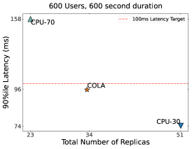
COLA Policies. In our evaluations we consider two COLA policies: ”COLA-50” and ”COLA-tail-100”. The ”COLA-50” policy is trained to scale microservice clusters with a median latency objective of 50 ms. The ”COLA-tail-100” policy targets 90%ile latency below 100ms. We include a full list of training hyperparameters and associated values for these policies in Table 15.
Terminology. We define the closest autoscaling policy as the policy whose latency is closest in absolute value to COLA. Secondly, we define the closest objective matching autoscaling policy as the most economical baseline policy which meets the median/tail latency objective. We use in sample to refer to request contexts that COLA and machine learned autoscalers have explicitly trained for and out of sample to refer to request contexts that these models have not observed in training, thus requiring COLA to interpolate. If COLA meets its latency target we compare directly with the closest objective matching autoscaling policy. If COLA does not meets its target we compare with the closest autoscaling policy.
5.3. Comparing Autoscaling Policies
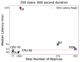
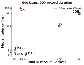
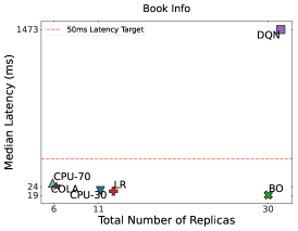
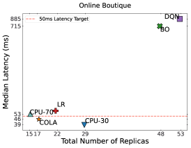
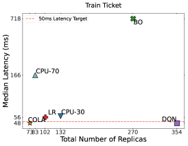
We examine the performance of COLA compared with baselines across the 5 microservices introduced in §5.1 and 4 workloads introduced in §5.1. For all applications we report evaluation numbers where half of the evaluated request per second rates are in-sample and half are out-of-sample. We summarize results and include full tabular results for all applications in Appendix tables 16–38.
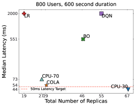
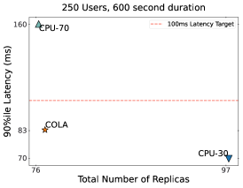
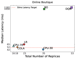
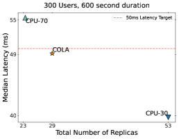
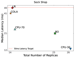
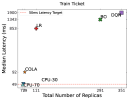
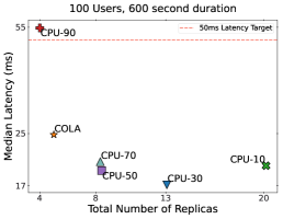
Constant Rate Workload. On all applications, COLA provides the lowest dollar cost autoscaling policy to meet our latency targets. We train and evaluate autoscalers on two latency targets, for 50 ms median latency and 100 ms tail latency. For the 50 ms median latency target, COLA costs 22.1% less than the next cheapest policy. When evaluated on a 100 ms tail latency target, COLA costs 20.8% less than the next cheapest policy. Across applications, workloads, and latency targets the closest autoscaling policy to COLA varies. This uncertainty in terms of which policy works best for a given setting indicates a key benefit of training an autoscaling policy. We show a few of these evaluations for the Online Boutique and Train Ticket applications in Figures 5-5 and detail a full set of tabular results in Appendix Tables 16–21.
Diurnal Workload. We evaluate autoscalers under a diurnal workload which consists of 5 different request per second rates run for 10 minutes each (a total of 3000 seconds). Both an in-sample and out-of-sample diurnal workload are run for each application. COLA produces the cheapest autoscaling policy for this diurnal workload for 3 out of 4 applications. On average COLA reduces costs by 20.1% compared to the next cheapest policy. On the Book Info application COLA is outperformed by the CPU-70 policy, costing 5% more than this policy. We show a few diurnal workloads in Figures 5-5 and include full results in Appendix Tables 22–26.
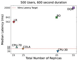
Unseen Request Distribution and Alternating Constant Rate Workloads. We evaluate COLA and CPU autoscalers on two additional workloads: (1) Unseen Request Distribution where the distribution of requests over operations is different from that seen at training time and (2) Alternating Constant Rate where the requests per second jumps immediately between a high and low request rate. For the Online Boutique application we train COLA on two different distributions of request workloads, one with a low frequency of purchasing an item and one with a frequency of purchases 3x higher, and evaluate on a third distribution with 2x the frequency of purchased orders. Results for this evaluation are shown in Figure 5. We find that COLA is able to reduce the cost of our cluster by 45.2% when compared to the CPU-30 autoscaler, the next cheapest policy, for this unseen request distribution. On the Sock Shop application we evaluate an alternating workload which switches between high and low request rates shown in Figure 5. We find COLA is able to reduce the cost of our cluster by 2.6% compared to the next cheapest policy, the CPU-70 autoscaler.
Performance across Cluster Architectures We evaluate COLA across a variety of cluster architectures. First, we alter the underlying VM sizes which host containers in our cluster. We find that COLA reduces cluster cost over the next best CPU or ML baseline by 21.6% for single core VMs, 12.4% for two core VMs, and 10.3% for four core VMs. As VM machine size increases granularity in resource allocation decisions play less of an effect on cost (e.g. in the extreme case where 1 large VM can host all containers, there is no way to reduce the cost a cloud tenant pays) and COLA provides less benefit over other policies. Secondly, we evaluate COLA on the newly introduced GKE Autopilot clusters, where users do not manage VMs but instead pay for only the aggregate pod requests made by launched containers. When compared with CPU baselines, we find that COLA reduces cost by 45.4% on Autopilot (Tables 36-38). Overall, we find that COLA consistently reduces costs across a set of different cluster configurations and offers the most benefits when deployed on Autopilot clusters.

5.4. Deconstructing COLA’s Gains
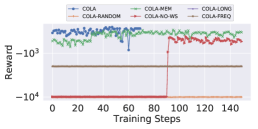
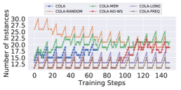
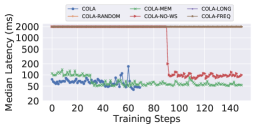
Service Selection. We find that selecting microservices for scaling by CPU utilization is crucial. In Figure 6 we compare replacing this selection heuristic with several other heuristics during training for the Online Boutique application. These heuristics are selecting services by memory utilization (COLA-MEM), randomly (COLA-RANDOM), without the warm starting optimization (COLA-WS), by the microservice with longest average span duration (COLA-LONG) and most frequently accessed microservice (COLA-FREQ). We find that these other heuristics take 1.58x–2.06x the amount of samples to train Online Boutique and 1.6x–12x the amount of samples to train Book Info (shown separately in Appendix Figure 24). Also, in most cases, replacing CPU utilization based service selection leads to policies which converge to a median latency above our target. This illustrates the importance of using domain knowledge in designing the right heuristic to train systems such as COLA. By contrast, applying machine learning to the autoscaling problem without the right heuristics, as our ML-based baselines do, yields poorer results. This can be seen in comparisons between COLA and ML-based baselines in Appendix Figures 22-23 where ML-based baselines often hit a wall in terms of reward or utilize drastically more resources to find policies which match our latency constraint. We take a deeper look at the gap between COLA and ML-based baselines in § 8.6.
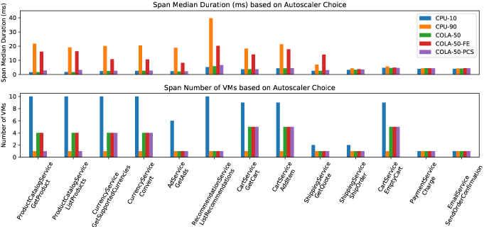
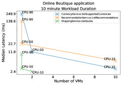
Scaling up Congested Microservices. We observe that COLA allocates more VMs to congested microservices by inspecting span-level microservice tracing data. We run an experiment in which we simulate 400 users for the Online Boutique application and compare COLA with underutilized (CPU-10) and overutilized (CPU-90) autoscaling policies. We collect tracing data from 4000 requests for each setting. In Figure 8 we sort the microservice spans from left to right in terms of decreasing congestion, defined as the percentage increase in span duration from the underutilized to overutilized setting. Microservices whose constituent spans have higher congestion, for example productcatalogservice, are the most benefited by COLA’s allocation of instances. As seen in Figure 8, COLA (shown in green) allocates more VMs to the microservices which are running these congested spans. As a result, COLA’s span durations are on average only 2.3% longer than CPU-10 with 65.8% fewer VMs.
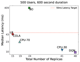
From our evaluations, we find that COLA outperforms machine learned autoscalers (Linear Regression, Bayesian Optimization and the Deep Q-Network) on all applications. We take a detailed look at the Online Boutique and find these approaches are not as successful as COLA in discerning congested microservices (discussed further in § 8.6). As a result these machine learned autoscalers allocate too many or too few resources to microservices which most heavily contribute to end to end latency (seen in Figures 16 and 17).
Tailoring a Policy to a Latency Target. We compare the policies COLA learns when trained to optimize median vs. 90%ile latency. For both of these latency targets, shown in Figure 7, we find that COLA has comparable median latency (47 and 46 ms respectively) across the different URL endpoints the Online Boutique application exposes. However we see 90%ile latency is reduced by close to 50% when COLA is trained to explicitly optimize 90%ile latency.
The largest difference between the two policies in terms of VM allocations is that COLA-tail-100 scales up the cartservice microservice with 5 as many instances as COLA-50. From Figure 7 we confirm that the two highest tail latency request URLs for the application relate to checking out and viewing the cart in Online Boutique. We find that COLA is able to tailor its policy to not only an application and workload but to a specified latency target itself as well.
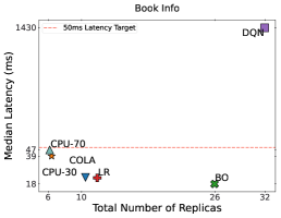
How close is COLA to optimal? We evaluate COLA for empirical optimality – finding the best possible cluster state for our given reward. For all applications and all workloads, we find that COLA is able to find a cluster state which meets our latency target. Since our latency target is met, we know that the only possible way to obtain a higher reward than COLA is to use fewer instances than COLA to meet the latency target. We exhaustively search all cluster states for Simple Web Server (which only has 30 possible states) and all cluster which use fewer instances than COLA for Book Info (which has 320,000 possible cluster states). We find that COLA finds the optimal cluster state in 9 of 10 total workload-application pairs and is the second best configuration when it was not optimal. Overall, COLA is .9% more expensive on average than the optimal configuration across these 10 evaluations. These results are shown in Appendix Figure 18.
5.5. Training Cost
To place the efficiency gains we’ve seen from using COLA in perspective, we review the cost to train our learned autoscaling policies. In Tables 3-7 we list these costs in terms of time, instances, and dollars needed to train a 50 ms median latency autoscaling policy for each application. These costs consider VMs in our application node pool, a second node pool for the ingress gateway and load balancer specific pods, and lastly the load generator itself. Virtual machines in the application node pool are n1-standard-1 machines which cost $.047 per hour, those in the load balancer node pool are e2-highmem-8 and cost $.361 per hour and our load generator operates on a custom defined 20 core, 52 GB mem machine which costs $.836 per hour.
| Application | Time (hrs) | Instance hrs | Cost ($) |
|---|---|---|---|
| Simple Web Server | 0.61 | 44.95 | $2.03 |
| Book Info | 0.65 | 58.04 | $2.64 |
| Online Boutique | 3.36 | 350.08 | $16.06 |
| Sock Shop | 1.34 | 193.21 | $8.95 |
| Train Ticket | 19.56 | 4772.43 | $223.39 |
In order to pay for the cost of COLA’s training, the system must decrease the instance hours used during deployment by at least as many instance hours as were used for training. For BookInfo, we would need to save roughly 58 instance hours to amortize cost and for Online Boutique we would need roughly 350 instance hours saved. For a 700 and 800 constant rate User/s workload in BookInfo, training cost is paid off in 19.3 and 8.6 hours respectively. In Online Boutique the 700 and 800 User/s workloads pay off training cost in 41.2 hours. For the Train Ticket application, training cost is paid off in 183.0 and 126.7 hours respectively for a 250 and 500 User/s workload respectively. Once training cost is paid, COLA results in a reduction in the cost of operating a microservice application. We include details and evaluations of model retraining in Appendix § 8.3.
6. Related Work
Scheduling. Several schedulers have been developed to manage how jobs are assigned to specific cluster resources such as Mesos (Hindman et al., 2011), Tarcil (Delimitrou et al., 2015), Omega (Schwarzkopf et al., 2013), Sparrow (Ousterhout et al., 2013), and Apollo (Boutin et al., 2014). These schedulers are designed to schedule jobs on clusters where the number of resources are fixed, not scale the cluster size dynamically as COLA does.
Automatically Selecting Number and Type of Cloud VMs. Various methods autoscale the number of physical or virtual machines based on current or forecasted resource demand such as Flexera (Flexera, [n.d.]), CloudScale (Shen et al., 2011), PRESS (Gong et al., 2010), and AGILE (Nguyen et al., 2013). These methods focus on the simpler setting of monoliths. Other projects optimize the type of VM instance based on application-specific knowledge and predictive algorithms; examples include Ernest (Venkataraman et al., 2016), CherryPick (Alipourfard et al., 2017) and PARIS (Yadwadkar et al., 2017). While COLA is built to specifically handle the challenges of microservice autoscaling, we adapt approaches inspired by Ernest (Venkataraman et al., 2016) and CherryPick (Alipourfard et al., 2017) for the microservice setting and compare to these adaptations.
Reward-Driven Autoscaling. Other works establish a Quality of Experience or Service metric that describes performance in a manner similar to COLA’s reward but do so for a general VM workload, not the microservice setting we target here. For instance, in (Ilyushkin et al., 2017), the authors analyze tradeoffs between a variety of horizontal autoscaling policies. In (Evangelidis et al., 2018), Evangelidis et. al constructs probabilistic rule based models for horizontal autoscaling in the public cloud.
Horizontal Autoscaling. In horizontal autoscaling, container-based cluster management tools such as Kubernetes (Kubernetes, [n.d.]c) allow users to scale the number of container pods based on utilization metrics. We compare COLA against the combination of the Kubernetes horizontal autoscaler and the GKE cluster autoscaler.
Vertical Autoscaling. In vertical autoscaling (Kubernetes, [n.d.]a), a controller maintains estimates of CPU and memory consumption of pods, scaling pods’ CPU and memory limits when they surpass a specified threshold. RUBAS (Rattihalli et al., 2019) extends this approach using a method which performs vertical autoscaling using the median and standard deviation of utilization metrics. Sinan (Zhang et al., 2021) is a recently proposed microservice vertical autoscaler which uses machine learning techniques to scale clusters by granularly allocating CPU cores. These procedures differ from COLA as their objective is to improve resource utilization of already allocated VMs—rather than reducing the dollar cost of adding VMs to microservices to meet an end-to-end latency target.
Autopilot. Autopilot (Rzadca et al., 2020) uses recommendation systems and past job utilization metrics to both predict and dynamically adjust pod limits. This autoscaling procedure differs from COLA in that the objective of Autopilot is to reduce slack (i.e., improve utilization) in the resources needed for a workload rather than navigating a latency-vs.-dollars tradeoff. The former objective is more aligned with the perspective of a cloud provider while the latter that of a cloud tenant. The authors of Autopilot also explicitly mention that the work does not optimize “serving jobs’ end user response latency”—a primary objective of COLA. To meet this objective at Google, the authors mention that serving workloads can be tuned in a manual and application-specific manner. We view COLA as an automated solution for such serving workloads.
Since the release of the Autopilot paper (Rzadca et al., 2020), Google has released a commercial offering called Autopilot, a ”node-less” version of Google Kubernetes Engine, on which developers can run a microservice application without having to rent Virtual Machines. In this setting, developers pay only for the aggregate pod requests in their application. We evaluate COLA and the Kubernetes HPA, which incorporates techniques presented in Autopilot, on the Autopilot platform. We show that COLA outperforms the Kubernetes HPA on all evaluations in Tables 36- 38.
Other Systems. Powerchief (Yang et al., 2017) uses queueing models to optimize the CPU frequencies of machines based on learned workload characteristics. This method’s procedure is primarily focused on reducing the energy cost of a cloud tenant for a desired performance rather than reducing the number of VMs. In Autotune (Chang et al., 2021), the authors propose a way to tune microservice cluster allocations. Autotune is complementary to autoscaling. It is meant for situations where the application is overprovisioned to begin with and can then be compacted to save cloud resources without losing performance. Lastly, FIRM (Qiu et al., 2020) learns to autoscale microservices using deep reinforcement learning. The approach hinges on providing this autoscaler with fine grained memory bandwidth and memory allocation information which requires hardware support (Intel Cache Allocation and Memory Bandwidth Allocation), unavailable in COLA’s cloud setting. Inspired by FIRM, we adapt a Deep Q-Network to operate with information available in our setting and compare COLA to it.
7. Conclusion
This paper presents COLA, a system for autoscaling microservice-based applications. While existing autoscalers scale each microservice within an application independently, COLA collectively decides how many VMs to allocate each microservice with the goal of achieving an end-to-end user latency target while minimizing dollar cost. Such a centralized approach to autoscaling gives COLA greater visibility into which microservices really matter for end-to-end latency and allows it to perform better than other approaches to microservice scaling that we compare against.
References
- (1)
- Alipourfard et al. (2017) Omid Alipourfard, Hongqiang Harry Liu, Jianshu Chen, Shivaram Venkataraman, Minlan Yu, and Ming Zhang. 2017. Cherrypick: Adaptively unearthing the best cloud configurations for big data analytics. In 14th USENIX Symposium on Networked Systems Design and Implementation (NSDI 17). 469–482.
- Amazon ([n.d.]) Amazon. [n.d.]. Amazon EKS - Managed Kubernetes Service. https://aws.amazon.com/eks/. (Accessed on 05/30/2020).
- Auer et al. (2002) Peter Auer, Nicolo Cesa-Bianchi, and Paul Fischer. 2002. Finite-time analysis of the multiarmed bandit problem. Machine learning 47, 2 (2002), 235–256.
- Barbeau and Kranakis (2007) Michel Barbeau and Evangelos Kranakis. 2007. Principles of ad-hoc networking. John Wiley & Sons.
- Boutin et al. (2014) Eric Boutin, Jaliya Ekanayake, Wei Lin, Bing Shi, Jingren Zhou, Zhengping Qian, Ming Wu, and Lidong Zhou. 2014. Apollo: Scalable and coordinated scheduling for cloud-scale computing. In 11th USENIX Symposium on Operating Systems Design and Implementation (OSDI 14). 285–300.
- Chang et al. (2021) Michael Alan Chang, Aurojit Panda, Hantao Wang, Yuancheng Tsai, Rahul Balakrishnan, and Scott Shenker. 2021. AutoTune: Improving End-to-end Performance and Resource Efficiency for Microservice Applications. arXiv preprint arXiv:2106.10334 (2021).
- Datadog ([n.d.]a) Datadog. [n.d.]a. 10 Trends in Real World Container Use — Datadog. https://www.datadoghq.com/container-report/. (Accessed on 06/01/2020).
- Datadog ([n.d.]b) Datadog. [n.d.]b. Datadog. https://www.datadoghq.com. (Accessed on 06/01/2020).
- Delimitrou et al. (2015) Christina Delimitrou, Daniel Sanchez, and Christos Kozyrakis. 2015. Tarcil: reconciling scheduling speed and quality in large shared clusters. In Proceedings of the Sixth ACM Symposium on Cloud Computing. 97–110.
- Evangelidis et al. (2018) Alexandros Evangelidis, David Parker, and Rami Bahsoon. 2018. Performance modelling and verification of cloud-based auto-scaling policies. Future Generation Computer Systems 87 (2018), 629–638.
- Flexera ([n.d.]) Flexera. [n.d.]. IT Management Software, Optimization & Solutions — Flexera. https://www.flexera.com/. (Accessed on 06/01/2020).
- Foundation ([n.d.]) The Linux Foundation. [n.d.]. OpenAPI Specification v3.1.0. https://spec.openapis.org/oas/latest.html.
- Gan et al. (2019) Yu Gan, Yanqi Zhang, Dailun Cheng, Ankitha Shetty, Priyal Rathi, Nayan Katarki, Ariana Bruno, Justin Hu, Brian Ritchken, Brendon Jackson, et al. 2019. An open-source benchmark suite for microservices and their hardware-software implications for cloud & edge systems. In Proceedings of the Twenty-Fourth International Conference on Architectural Support for Programming Languages and Operating Systems. 3–18.
- gevent Coroutine-based concurrency library for Python ([n.d.]) gevent Coroutine-based concurrency library for Python. [n.d.]. https://github.com/gevent/gevent. https://github.com/gevent/gevent. (Accessed on 06/01/2020).
- Gong et al. (2010) Zhenhuan Gong, Xiaohui Gu, and John Wilkes. 2010. Press: Predictive elastic resource scaling for cloud systems. In 2010 International Conference on Network and Service Management. Ieee, 9–16.
- Google ([n.d.]a) Google. [n.d.]a. Find out how you stack up to new industry benchmarks for mobile page speed. https://www.thinkwithgoogle.com/marketing-strategies/app-and-mobile/mobile-page-speed-new-industry-benchmarks/.
- Google ([n.d.]b) Google. [n.d.]b. Kubernetes - Google Kubernetes Engine (GKE) — Google Cloud. https://cloud.google.com/kubernetes-engine. (Accessed on 05/30/2020).
- Google ([n.d.]c) Google. [n.d.]c. Online Boutique Application. https://github.com/GoogleCloudPlatform/microservices-demo.
- Grassmann (1983) W Grassmann. 1983. The convexity of the mean queue size of the M/M/c queue with respect to the traffic intensity. Journal of Applied Probability 20, 4 (1983), 916–919.
- Grassmann (1981) Winfried K Grassmann. 1981. Stochastic systems for management. New York: North Holland.
- Hindman et al. (2011) Benjamin Hindman, Andy Konwinski, Matei Zaharia, Ali Ghodsi, Anthony D Joseph, Randy H Katz, Scott Shenker, and Ion Stoica. 2011. Mesos: A platform for fine-grained resource sharing in the data center.. In NSDI. 22–22.
- Homescu et al. (2013) Andrei Homescu, Steven Neisius, Per Larsen, Stefan Brunthaler, and Michael Franz. 2013. Profile-guided automated software diversity. In Proceedings of the 2013 IEEE/ACM International Symposium on Code Generation and Optimization (CGO). IEEE, 1–11.
- Ilyushkin et al. (2017) Alexey Ilyushkin, Ahmed Ali-Eldin, Nikolas Herbst, Alessandro V Papadopoulos, Bogdan Ghit, Dick Epema, and Alexandru Iosup. 2017. An experimental performance evaluation of autoscaling policies for complex workflows. In Proceedings of the 8th ACM/SPEC on International Conference on Performance Engineering. 75–86.
- Istio ([n.d.]a) Istio. [n.d.]a. Istio / Bookinfo Application. https://istio.io/latest/docs/examples/bookinfo/.
- Istio ([n.d.]b) Istio. [n.d.]b. Istio Hello World Sample Microservice. https://github.com/istio/istio/tree/master/samples/helloworld. (Accessed on 05/30/2020).
- Jaeger ([n.d.]) Jaeger. [n.d.]. Jaeger: open source, end-to-end distributed tracing. https://www.jaegertracing.io/. (Accessed on 06/01/2020).
- Kubernetes ([n.d.]a) Kubernetes. [n.d.]a. community/vertical-pod-autoscaler.md at master · kubernetes/community. https://github.com/kubernetes/community/blob/master/contributors/design-proposals/autoscaling/vertical-pod-autoscaler.md. (Accessed on 06/01/2020).
- Kubernetes ([n.d.]b) Kubernetes. [n.d.]b. Kubernetes Cluster Autoscaler - FAQ. https://github.com/kubernetes/autoscaler/blob/master/cluster-autoscaler/FAQ.md#what-is-cluster-autoscaler.
- Kubernetes ([n.d.]c) Kubernetes. [n.d.]c. Production-Grade Container Orchestration - Kubernetes. https://kubernetes.io/. (Accessed on 05/30/2020).
- Langford and Zhang (2007) John Langford and Tong Zhang. 2007. The epoch-greedy algorithm for contextual multi-armed bandits. Advances in neural information processing systems 20, 1 (2007), 96–1.
- Lattner (2002) Chris Arthur Lattner. 2002. LLVM: An infrastructure for multi-stage optimization. Ph.D. Dissertation. University of Illinois at Urbana-Champaign.
- Li et al. (2014) Jialin Li, Naveen Kr Sharma, Dan RK Ports, and Steven D Gribble. 2014. Tales of the tail: Hardware, os, and application-level sources of tail latency. In Proceedings of the ACM Symposium on Cloud Computing. 1–14.
- Lillicrap et al. (2015) Timothy P Lillicrap, Jonathan J Hunt, Alexander Pritzel, Nicolas Heess, Tom Erez, Yuval Tassa, David Silver, and Daan Wierstra. 2015. Continuous control with deep reinforcement learning. arXiv preprint arXiv:1509.02971 (2015).
- Little and Graves (2008) John DC Little and Stephen C Graves. 2008. Little’s law. In Building intuition. Springer, 81–100.
- Locust ([n.d.]) Locust. [n.d.]. Locust Load Generator. https://locust.io/.
- Microsoft ([n.d.]) Microsoft. [n.d.]. Azure Kubernetes Service (AKS) — Microsoft Azure. https://azure.microsoft.com/en-us/services/kubernetes-service/. (Accessed on 05/30/2020).
- Netflix ([n.d.]) Netflix. [n.d.]. Microservices Workshop - Craft Conference. https://www.slideshare.net/adriancockcroft/microservices-workshop-craft-conference.
- Nguyen et al. (2013) Hiep Nguyen, Zhiming Shen, Xiaohui Gu, Sethuraman Subbiah, and John Wilkes. 2013. AGILE: Elastic Distributed Resource Scaling for Infrastructure-as-a-Service. In Proceedings of the 10th International Conference on Autonomic Computing (ICAC 13). 69–82.
- OpenTracing ([n.d.]) OpenTracing. [n.d.]. OpenTracing Specification v1.1. https://opentracing.io/specification/.
- Ousterhout et al. (2013) Kay Ousterhout, Patrick Wendell, Matei Zaharia, and Ion Stoica. 2013. Sparrow: distributed, low latency scheduling. In Proceedings of the Twenty-Fourth ACM Symposium on Operating Systems Principles. 69–84.
- Patwardhan et al. (2004) Jaidev P Patwardhan, Alvin R Lebeck, and Daniel J Sorin. 2004. Communication breakdown: analyzing cpu usage in commercial web workloads. In IEEE International Symposium on-ISPASS Performance Analysis of Systems and Software, 2004. IEEE, 12–19.
- Pedregosa et al. (2011) F. Pedregosa, G. Varoquaux, A. Gramfort, V. Michel, B. Thirion, O. Grisel, M. Blondel, P. Prettenhofer, R. Weiss, V. Dubourg, J. Vanderplas, A. Passos, D. Cournapeau, M. Brucher, M. Perrot, and E. Duchesnay. 2011. Scikit-learn: Machine Learning in Python. Journal of Machine Learning Research 12 (2011), 2825–2830.
- Qiu et al. (2020) Haoran Qiu, Subho S Banerjee, Saurabh Jha, Zbigniew T Kalbarczyk, and Ravishankar K Iyer. 2020. FIRM: An Intelligent Fine-grained Resource Management Framework for SLO-Oriented Microservices. In 14th USENIX Symposium on Operating Systems Design and Implementation (OSDI 20). 805–825.
- Rattihalli et al. (2019) Gourav Rattihalli, Madhusudhan Govindaraju, Hui Lu, and Devesh Tiwari. 2019. Exploring Potential for Non-Disruptive Vertical Auto Scaling and Resource Estimation in Kubernetes. In 2019 IEEE 12th International Conference on Cloud Computing (CLOUD). IEEE, 33–40.
- Rzadca et al. (2020) Krzysztof Rzadca, Pawel Findeisen, Jacek Swiderski, Przemyslaw Zych, Przemyslaw Broniek, Jarek Kusmierek, Pawel Nowak, Beata Strack, Piotr Witusowski, Steven Hand, et al. 2020. Autopilot: workload autoscaling at Google. In Proceedings of the Fifteenth European Conference on Computer Systems. 1–16.
- Schwarzkopf et al. (2013) Malte Schwarzkopf, Andy Konwinski, Michael Abd-El-Malek, and John Wilkes. 2013. Omega: flexible, scalable schedulers for large compute clusters. In Proceedings of the 8th ACM European Conference on Computer Systems. 351–364.
- Shen et al. (2011) Zhiming Shen, Sethuraman Subbiah, Xiaohui Gu, and John Wilkes. 2011. Cloudscale: elastic resource scaling for multi-tenant cloud systems. In Proceedings of the 2nd ACM Symposium on Cloud Computing. 1–14.
- Slivkins (2019) Aleksandrs Slivkins. 2019. Introduction to multi-armed bandits. arXiv preprint arXiv:1904.07272 (2019).
- Twitter ([n.d.]) Twitter. [n.d.]. Decomposing Twitter Adventures in Service Oriented Architecture. https://www.slideshare.net/InfoQ/decomposing-twitter-adventures-in-serviceoriented-architecture.
- Uber ([n.d.]) Uber. [n.d.]. Microservice Architecture. https://eng.uber.com/microservice-architecture/.
- Venkataraman et al. (2016) Shivaram Venkataraman, Zongheng Yang, Michael Franklin, Benjamin Recht, and Ion Stoica. 2016. Ernest: Efficient performance prediction for large-scale advanced analytics. In 13th USENIX Symposium on Networked Systems Design and Implementation (NSDI 16). 363–378.
- Vulimiri et al. (2013) Ashish Vulimiri, Philip Brighten Godfrey, Radhika Mittal, Justine Sherry, Sylvia Ratnasamy, and Scott Shenker. 2013. Low latency via redundancy. In Proceedings of the ninth ACM conference on Emerging networking experiments and technologies. 283–294.
- Weaveworks ([n.d.]) Weaveworks. [n.d.]. Sock Shop Application. https://github.com/microservices-demo/microservices-demo. (Accessed on 05/30/2020).
- Yadwadkar et al. (2017) Neeraja J Yadwadkar, Bharath Hariharan, Joseph E Gonzalez, Burton Smith, and Randy H Katz. 2017. Selecting the best vm across multiple public clouds: A data-driven performance modeling approach. In Proceedings of the 2017 Symposium on Cloud Computing. 452–465.
- Yang et al. (2017) Hailong Yang, Quan Chen, Moeiz Riaz, Zhongzhi Luan, Lingjia Tang, and Jason Mars. 2017. Powerchief: Intelligent power allocation for multi-stage applications to improve responsiveness on power constrained cmp. In Proceedings of the 44th Annual International Symposium on Computer Architecture. 133–146.
- Yanqi et al. ([n.d.]) Zhang Yanqi, Hua Weizhe, Zhou Zhuangzhuang, Suh G. Edward, and Delimitrou Christina. [n.d.]. Sinan Google Cloud Platform Release. https://github.com/zyqCSL/sinan-gcp.
- Zhang et al. (2021) Yanqi Zhang, Weizhe Hua, Zhuangzhuang Zhou, G Edward Suh, and Christina Delimitrou. 2021. Sinan: ML-based and QoS-aware resource management for cloud microservices. In Proceedings of the 26th ACM International Conference on Architectural Support for Programming Languages and Operating Systems. 167–181.
- Zhou et al. (2018) Xiang Zhou, Xin Peng, Tao Xie, Jun Sun, Chenjie Xu, Chao Ji, and Wenyun Zhao. 2018. Poster: Benchmarking microservice systems for software engineering research. In 2018 IEEE/ACM 40th International Conference on Software Engineering: Companion (ICSE-Companion). IEEE, 323–324.
- Zipkin ([n.d.]) Zipkin. [n.d.]. OpenZipkin · A distributed tracing system. https://zipkin.io/. (Accessed on 06/01/2020).
8. Appendix
8.1. Queueing Theory Analysis
We model each microservice as an M/M/c queue. In this case, we assume arrivals form a single queue and are governed by a Poisson process with rate , that there are c servers, and job service times are exponentially distributed with parameter . The response time can be composed into two pieces: a queueing time and service time. The service time is fixed, , and consequently latency is increased/decreased by increasing/decreasing the queueing time. This queueing time is shown below and is based on Erlang’s C formula (Barbeau and Kranakis, 2007) which governs the number of customers in an M/M/c queue given a number of servers and utilization, .
| (2) |
In addition to the formula above, for an M/M/c queue, we have the queuing length , which is a result of Little’s Law (Little and Graves, 2008). Lastly, is the probability that all servers are busy. The expected number of busy servers is and is no larger than (Grassmann, 1981).
We refer readers to (Barbeau and Kranakis, 2007) for a more detailed treatment of the behavior of queuing theory.
Proposition 1.
Consider a set of M/M/c queues with utilization . Further, let us say that M/M/c queues have the same . Increasing the number of servers for the highest utilized M/M/c queue, the queue associated with , has the greatest upper bound in terms of queuing length reduction.
We rely on the convexity of M/M/c queuing length with respect to . This property is well known and shown in a previous paper by Grassmann (Grassmann, 1983). As a direct result of this convexity, we know the following is true:
| (3) |
Let us consider the case in which we add a server (increasing to ) to our M/M/c queue with and fixed. We can let be the case with servers and be the case with servers.
All terms above are increasing in . Consequently, choosing to add a server to the most utilized M/M/c queue offers the greatest upper bound in terms of queue length reduction: . Since queuing time, , simply equals , adding a server to the most utilized M/M/c queue also offers the greatest upper bound in terms of queuing time reduction with equal across our queues.
Proposition 2.
Consider a linearly interpolating policy between and corresponding to input rates and where . We assume that under both and , the queuing delay satisfies a latency target. We show that in some cases this latency from an interpolated policy of these two policies maintains or reduces queuing delay and consequently achieves the latency target we desire. At most the linear interpolation policy increases queuing delay by , a ratio which may be controlled by altering the spacing of the considered policies.
Let us consider the two possible cases under which we perform linear interpolation between and . These cases are: (1) and (2) . We denote the interpolated utilization as .
In the first case where , denote . We know that since:
The last line is a result of which is true since we are interpolating between two endpoints and .
We begin with a result from Proposition 1 to show our claim that . Note that with and positive, we have positive.
With , we have and that . Let where .
Since , we have obtained the desired result: when .
For the second case we consider when . By the same argument as for our first case, we know that within our interpolating range.
Let where .
Since we know . Consequently, we know that is at most larger than as well as our target queuing delay.
8.2. Further Evaluations
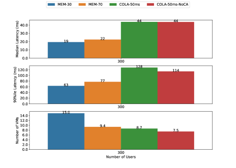
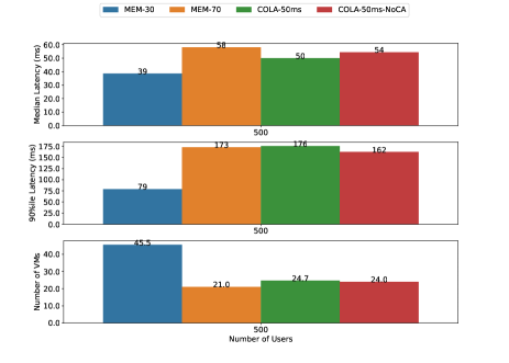
Constant Rate Workloads In Figures 12 and 12 we show constant rate evaluations for the Book Info and Sock Shop applications. For the BookInfo application, we train COLA on 200, 400, 600 and 800 requests per second with a target of 50ms median latency. It is asked to autoscale for fixed rate workloads both in and out of our training samples; shown in Figure 11. COLA provides the most cost effective policy across all candidate autoscalers with the next cheapest policy (CPU-70) costing 28.5% more. For the Sock Shop application we train COLA on 200, 300, 400, and 500 requests per second for a median latency of 50ms. On a set of in sample workloads we find that the most cost effective autoscaling policy depends on the workload (Figure 12). Overall, COLA is the cheapest policy to meet the latency target across all workloads. Tables 16 and 17 detail the full results of these experiments.
In Sample Diurnal Workloads Figure 12 shows In-Sample diurnal workloads for the Book Info, Online Boutique and Train Ticket applications. On the Book Info application, COLA meets its latency target but is outperformed by the CPU-70 policy with a cost reduction of -3%. For the Online Boutique application, COLA reduces cost over the next cheapest policy which meets the target, CPU-30, by 46%. For the Train Ticket application, COLA performs worse on the In Sample diurnal workload compared to the CPU-30 and CPU-70 policies. It incurs a cost reduction of -7.4%. Tables 23, 22, and 25 show the numerical results of these experiments.
Large Dynamic Request Range For our evaluations we have trained and evaluated autoscalers on a dynamic request range – the ratio between the largest and smallest number of requests – of 4 to 5 depending on the application. Realistically, this dynamic request range could be much higher if the use of an application fluctuates significantly (e.g. based on the time of day). We run evaluations where COLA is trained and then manages a cluster across a dynamic request range of 40, with the smallest number of requests being 25 and the largest being 1000. Results for this setting are shown below in Figure 12 and compared to a variety of CPU threshold autoscalers. Across six different request rates, COLA reduces the cost to meet our 50ms latency objective by 24.2%. Tabular results for this evaluation are listed in Table 29.
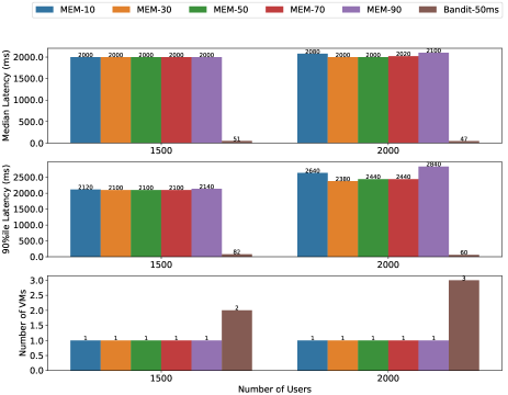
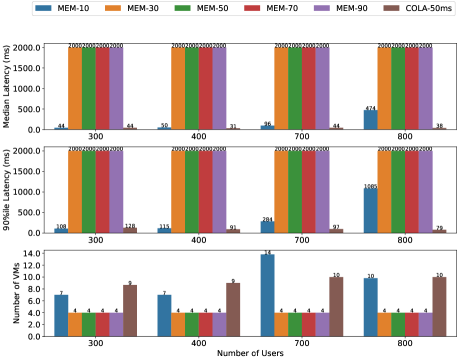
Memory Threshold Autoscaling Policies We include Constant Rate evaluations which compare COLA with a variety of memory threshold autoscalers. For the applications on which we evaluate, we find that memory threshold autoscalers offer worse and/or inconsistent performance compared to CPU threshold autoscalers and consequently present them here in the Appendix.
For the Simple Web Server application, memory autoscaler only perform well on the 500 request per second case as only 1 node is needed to satisfy the load. In all other workloads, the memory autoscalers fail to scale up to the incoming load.
In the Book Info application, only the 10% memory autoscaler scales up microservice replicas and performs well for the 300 and 400 request per second. However, for 700 and 800 requests per second the memory autoscaler suffers high median and tail latencies for all thresholds.
For the Online Boutique Application, memory autoscalers fail to scale up to the workloads and suffer poor median and tail latencies.
8.3. Model Retraining
Over time, production workloads may drift outside our training request per second range and/or request distribution. We show training cost associated with adding a new workload and modifying the latency target for COLA. Generally, we note that model retraining for a new specification will depend significantly on the application and workload. Several triggers can be applied to retrain COLA, for example observing latency higher than the target, number of times COLA falls back to another autoscaler, or percent of requests which return errors. For context, Autopilot’s authors (Rzadca et al., 2020) note that a few anecdotal applications at Google are reconfigured roughly 10 times a month.
| Add Workload | Update Latency | |||
|---|---|---|---|---|
| Application | Time | Cost ($) | Time | Cost ($) |
| Simple Web Server | 0.18 | $0.59 | 0.31 | $1.02 |
| Book Info | 0.19 | $0.77 | 0.27 | $1.09 |
| Online Boutique | 0.28 | $2.03 | 0.31 | $1.49 |
| Train Ticket | 0.51 | $5.83 | 0.54 | $6.12 |
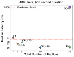
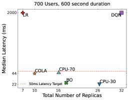
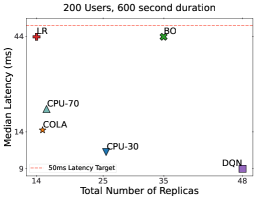
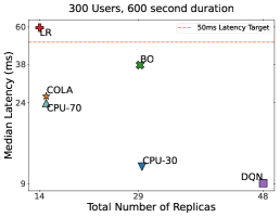

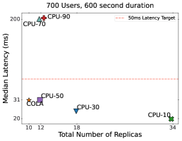
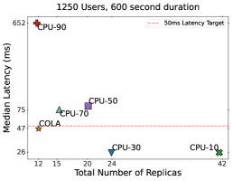
8.4. Model Robustness
Control Lag and Measurement Noise All autoscalers we evaluate operate a control loop. Some measurement is input to the controller at which point the controller will take an action to progress towards a set point of interest. In COLA the total requests per second along with a distribution of requests across operations are the input to the controller. The set point our controller guides toward is the cluster state associated with this measurement input. We examine two sources of error in this control loop: controller input lag and sensor noise.
For COLA, there is a lag between when a workload changes (e.g. aggregate RPS increases) and our controller is notified of this change. For our evaluation setting, workload metrics are logged by Google Cloud Monitoring agents. We use the default logging settings provided by Google Cloud for all experiments which means agents that collect and write new logs pertaining to requests do so every 60 seconds.
To better understand the effect of this input lag, we run an experiment where we invoke a load change from no load to a new request per second rate. To isolate this input lag, in this experiment virtual machines have been pre-allocated and autoscalers must simply increase the number of pods in response to an input load. We observe that it takes between 60-90 seconds to react to a load change once a workload has changed enough to warrant action. Although COLA takes longer to start scaling up compared to CPU threshold based autoscaling policies, the cluster state for the new workload and corresponding latency reaches a steady state more quickly.
Secondly, the number of requests we log can be a source of noise. In our settings we empirically find this to not be the case. We evaluate the mean average percent error (MAPE) of five 1-minute intervals of a workload against our measurement taken during training to build our context. The MAPE for Online Boutique, BookInfo and Hello World are .58%, .34% and 1.1% respectively.
Sample Duration and Measurement Variation We evaluate the selection of a training procedure hyperparameter: sample duration. The duration of our samples can determine the impact of transient noise on our reward estimation during training. Longer training times can help reduce the variance in latency and reward estimation for a fixed cluster configuration and request rate as we average latency over more samples. However, taking longer samples increases the dollar cost of training since we will run a training cluster for a longer period of time. In Figure 15, we show the sample estimation error as it relates to sample duration on one configuration of the Online Boutique application. We calculate the mean percent error of various sample durations from 10 to 80 seconds against a ground truth held out sample of 90 seconds.
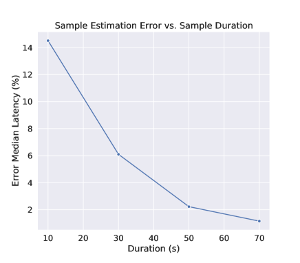
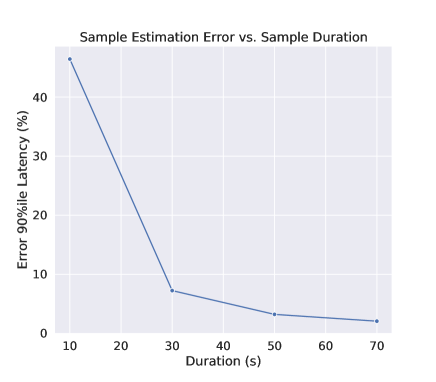
Other robustness experiments We evaluate a few other settings to further understand failure cases and extensibility of COLA. We evaluate out of range workloads in which we issue a request per second rate larger than the upper bound that COLA is trained for. COLA fails over to a preset Kubernetes CPU autoscaling threshold as shown in Figure 19. Additionally, we show the coexistence of COLA’s horizontal pod autoscaler with GKE’s cluster autoscaler on the Book Info and Online Boutique applications in Figures 14 and 14.
8.5. Learned Autoscaler Training Times
We show the training time for learned autoscalers apart from COLA in Tables 3-7. The Linear Regression, Bayesian Optimization and Deep Q-Network learned autoscaling policies use more instance hours time during training. Since the space of microservice configurations is explored in ascending size across training samples COLA allocates only a fraction of the full instances needed for the maximum replica range. During training, if the number of replicas grows we add more instances to the training node pool. Both DQN and Bayesian Optimization operate by freely exploring the entire replica range with each subsequent training example requesting an arbitrary number of instances. Consequently we can not perform this optimization for these policies. For the Linear Regression policy we know the full set of training examples before training and consequently a version of this optimization can be performed. The optimization procedure for Linear Regression could sort the full set of training examples by ascending resources requested and incrementally increase the cluster size.
| Application | Time (hrs) | Instance Hrs | Cost ($) |
|---|---|---|---|
| Simple Web Server | 4.16 | 308.33 | $13.94 |
| Book Info | 3.89 | 346.11 | $15.79 |
| Online Boutique | 5.03 | 874.00 | $40.68 |
| Sock Shop | 6.94 | 1000.00 | $46.33 |
| Train Ticket | 7.29 | 5060.42 | $239.14 |
| Application | Time (hrs) | Instance Hrs | Cost ($) |
|---|---|---|---|
| Simple Web Server | 4.19 | 309.88 | $14.01 |
| Book Info | 3.91 | 406.47 | $18.65 |
| Online Boutique | 5.86 | 1020.08 | $47.46 |
| Sock Shop | 6.98 | 1005.00 | $46.56 |
| Train Ticket | 7.32 | 5080.66 | $240.09 |
| Application | Time (hrs) | Instance Hrs | Cost ($) |
|---|---|---|---|
| Simple Web Server | 4.22 | 312.72 | $14.14 |
| Book Info | 3.96 | 412.44 | $18.92 |
| Online Boutique | 5.96 | 1156.84 | $53.95 |
| Sock Shop | 7.07 | 1018.08 | $47.17 |
| Train Ticket | 7.81 | 5579.94 | $263.73 |
8.6. Analyzing Learned Autoscaler Shortcomings
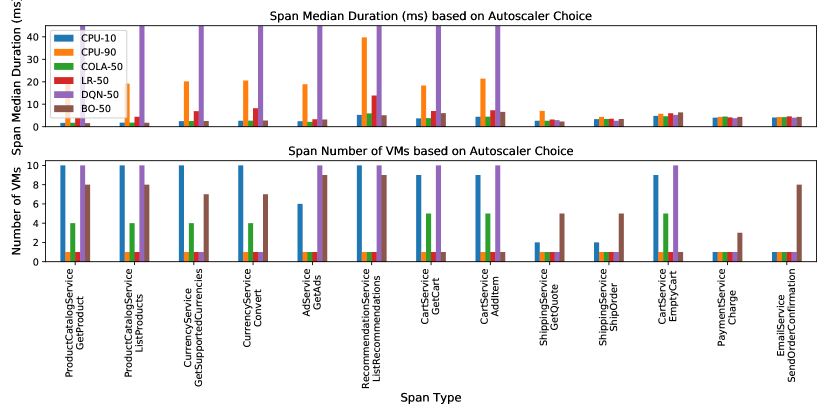
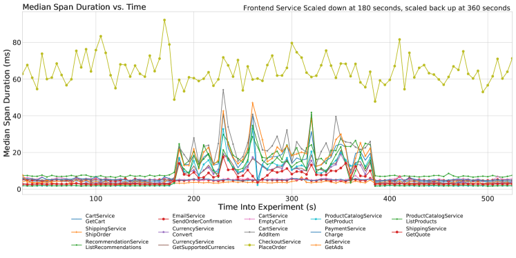
| Autoscaler | Median Span Duration (ms) | Num Instances |
|---|---|---|
| CPU-10 | 3.30 | 85 |
| CPU-90 | 15.81 | 13 |
| COLA-50 | 3.41 | 26 |
| LR-50 | 5.86 | 15 |
| BO-50 | 3.84 | 81 |
| DQN-50 | 117.74 | 65 |
We analyze the scaling decisions of COLA in relation to other learned autoscaling policies - Linear Regression, Bayesian Optimization and Deep Q-Learning. COLA outperforms these benchmarks on all applications. In Figure 16 we show span durations and number of instances for the Online Boutique application with 400 synthetic users. Table 8 shows a summary of median latency and total number of instances for these policies.
We find that Linear Regression and Deep Q-Learning result in higher span durations than COLA. In these two cases, the policies allocated 32.6% and 85.7% fewer frontend instances than COLA. As detailed in controlled experiments from §5 (Figure 8), the frontend instance has downstream latency effects on several other microservices. We perform another controlled experiment to show this effect which can be seen in Figure 17. In this Figure, we show a timeseries of several spans in our microservice. The first and last 180 seconds in the experiment we apply COLA’s policy. The middle 180 seconds we scale down the frontend to CPU-90’s value. From the figure we can observe that while some spans are uneffected in duration from this policy change, the majority of spans rise in latency as a result of scaling down the upstream frontend service. Lastly, the Bayesian Optimization autoscaler results in similar span duration to COLA but expends 3.1 the resources that COLA does. Generally, we observe that our learned autoscaling baselines either allocate too few or too many resources to our microservice cluster. COLA relies on system heuristics in addition to machine learning to prioritize resource allocation to microservices which reduce end to end latency significantly.
8.7. Training Trajectory Visualizations
In Figures 22-23 we show the evolution of learned policies during training for our machine learned autoscalers. For COLA, DQN, and Linear Regression we train on the same set of RPS values in our range and compare latency, number of instances and reward as a function of training samples for each of these RPS values. Across the applications tested, we find that COLA is able to converge to a latency which meets our target faster than other machine learned autoscalers. Further, COLA reaches a steady state reward which is better or equal to other autoscalers for all RPS values we examine.
8.8. Service Selection
In Figure 24, we show the effect of altering service selection, a routine described in §3.2, on the Bookinfo application. For all applications COLA chooses services to optimize by prioritizing those with high CPU utilization. We also show in Figure 24 training trajectories where we instead select services by high memory utilization (COLA-mem) and where we select services randomly (COLA-random). We find that in our setting, prioritizing the optimization of services high in CPU utilization works best with autoscalers more quickly finding satisfactory configurations for provided workloads. This may be heavily influenced by our selection of applications which are latency sensitive web applications.
8.9. Reducing Collateral Damage from Congestion.
From Figure 8, we notice that COLA also reduces the duration of spans on microservices which are not scaled up. We find that this benefit comes from reducing the latency of other spans, which are dependencies of these non-scaled-up spans. As noted in DeathStarBench (Gan et al., 2019), microservice applications are difficult to optimize as congested upstream microservices can cause “hotspots” and introduce queueing delays to downstream microservices as well. We deploy a version of the COLA autoscaling policy, shown in Figure 8 as ”COLA-50-FE”, where we scale down the frontend microservice (which is upstream to all microservices) to the same number of VMs as the overutilized CPU-90 policy. We observe that the span durations increase for almost every span as a result of scaling down only the frontend.
Secondly, DeathStarBench (Gan et al., 2019) documents how backpressure can occur when an upstream microservice span blocks and waits for a reply from a downstream microservice. We find a case of this type of behavior in the Online Boutique microservice code where the recommendationservice code fetches a list of products from the productcatalogservice, blocking until this list is received. We run a second modified version of COLA where we scale down the productcatalog service to the same value as CPU-90, the overutilized system. As a result the listproducts span duration increases by 85% (or 1.5ms). Although the resources available to the recommendationservice are unchanged, the list
recommendations span duration increases by .85 ms or 13% of the total span duration. This illustates the benefits of COLA’s global visibility: it observes the consequences on end-to-end latency of each VM allocation choice it makes.
8.10. COLA Empirical Optimality
We show evaluation of COLA for empirical optimality – finding the best possible cluster state for our given reward. Figure 18 shows the reward for each cluster state searched with COLA’s solution in orange and all other cluster states in blue. We run each workload for 90 seconds per cluster state and calculate reward for a median latency target of 50ms. COLA is optimal for 9/10 application-workload pairs which we evaluated and is the second best configuration on the last pair. COLA has been trained on 6/10 of these evaluated application-workload pairs and has not seen 4/10. COLA costs .9% more on average than the optimal cluster state across these experiments.
During training, COLA takes 10 samples per workload for the Simple Web Server application and 13.3 samples on average per workload for Book Info. In total there are 30 possible cluster states for the Simple Web Server application and 320,000 for the Book Info application. We compare the search strategy used by COLA with random search and Bayesian Optimization which we allot 10 samples per workload for the Simple Web Server application (1x COLA’s number of samples) and 40 samples for the Book Info application (3x COLA’s number of samples). The random search procedure takes the alloted samples and chooses the best configuration out of the samples for the workload. Bayesian Optimization is implemented as a Gaussian Process Regressor with a feature vector consisting of number of replicas for each microservice. We train a seperate model per workload, using the implementation from the scikit-learn package (Pedregosa et al., 2011). Overall, we find that COLA significantly outperforms both random search and Bayesian Optimization and show results in Tables 9 and 10.
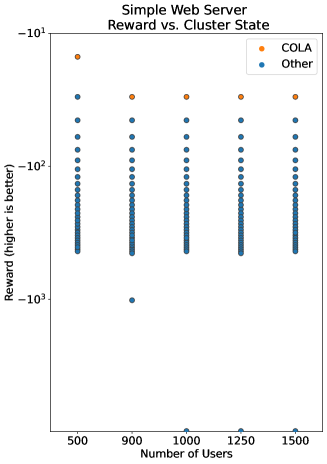
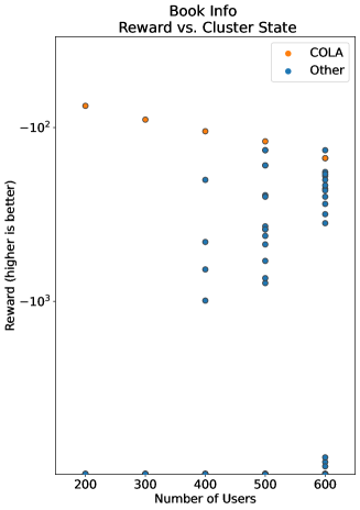
8.11. Failed Requests across Workloads
In Tables 16-28 we include the failed requests per second across all workloads on which we evaluate. For CPU autoscalers and COLA we observe fewer than .1% of requests being timed out by the client except for in one case for the Train Ticket application. During training and evaluation, requests may respond with a 4xx or 5xx response code and are consequently registered as a failed request. For example, a request may timeout at the client or microservice cluster and be considered a failed request.
During both training and evaluation we use a timeout of 2000ms on the client side and 30 seconds on the server. This timeout is applied for a few reasons. Firstly, we send requests through a connection pool in which each connection is able to issue a request at a given interval which will decide the aggregate requests per second issued to the cluster. If timeout limits are unbounded we must adjust the size of the connection pool. In order to avoid arbitrarily opening new connections we apply a timeout, , for the connection pool. This value is also the interval at which we send requests for each connection. In order to issue an aggregate number of requests per second, , to our cluster we adjust the number of connections in our pool once on startup to . During evaluation we retain this client side timeout which in this case has a second purpose – to mimic user requests ”bouncing” after some significant waiting time. The amount of time a user waits to ”bounce” and reissue a request can depend heavily by application among other factors. However, we find that the timeout we specify is roughly in line with the average bounce time in modern web applications based on an industry benchmark from Google (Google, [n.d.]a).
| Autoscaler | Users | Reward | Latency | Replicas |
|---|---|---|---|---|
| COLA-50 | 500 | -15.0 | 46.0 | 1.0 |
| Random | 500 | -60.0 | 45.0 | 4.0 |
| Bayesian Opt. | 500 | -15.0 | 46.0 | 1.0 |
| COLA-50 | 1000 | -30.0 | 50.0 | 2.0 |
| Random | 1000 | -60.0 | 46.0 | 4.0 |
| Bayesian Opt. | 1000 | -225.0 | 45.0 | 15.0 |
| COLA-50 | 1500 | -30.0 | 50.0 | 2.0 |
| Random | 1500 | -30.0 | 50.0 | 2.0 |
| Bayesian Opt. | 1500 | -240.0 | 45.0 | 16.0 |
| Autoscaler | Users | Reward | Latency | Replicas |
|---|---|---|---|---|
| COLA-50 | 200 | -75.0 | 30.0 | 5.0 |
| Random | 200 | -210.0 | 33.0 | 14.0 |
| Bayesian Opt. | 200 | -660.0 | 37.0 | 44.0 |
| COLA-50 | 400 | -105.0 | 38.0 | 7.0 |
| Random | 400 | -210.0 | 36.0 | 14.0 |
| Bayesian Opt. | 400 | -180.0 | 31.0 | 12.0 |
| COLA-50 | 600 | -150.0 | 45.0 | 10.0 |
| Random | 600 | -255.0 | 56.0 | 15.0 |
| Bayesian Opt. | 600 | -480.0 | 53.0 | 31.0 |
Although our latency based timeout is respected in the vast majority of experiments, we find one such experiment where this is not true (in Table 18). Locust (Locust, [n.d.]), the load generator we use to issue requests and collect aggregate statistics, uses an http client exposed by the gevent (gevent Coroutine-based concurrency library for Python, [n.d.]) library for all of our experiments. Within the source code of this library, the authors mention that there may be a ”fuzz” in the time taken to interrupt the http client for a specific timeout. This fuzz can cause the maximum latency to be larger than the timeout specified and inevitably occurs due to resource contention. For our setting, this fuzz in handling timeout operations effects very few evaluations. Further, it only effects the worst autoscaling policies for a given application and workload.
8.12. Out of Range Evaluation
We evaluate the graceful failover in COLA for the Online Boutique application. We train with an upper limit of 200 users and ask COLA to fail over to a 50% CPU based autoscaling policy when the observed requests are at least 30% larger than the largest context it has trained on. The results of one evaluation when 600 users request the system are shown below. In Figure 19 we can see the scaling up of instances and median latency as COLA transitions to a CPU autoscaler.
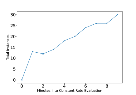
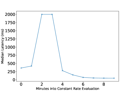
8.13. Coexistence with GKE Cluster Autoscaler
We evaluate a few Constant Rate workloads with Google Kubernetes Engine handling the cluster autoscaling and COLA handling horizontal pod autoscaling for Book Info in Figure 14 and Online Boutique in Figure 14. Performance is comparable between the cluster autoscaler we develop and the cluster autoscaler offered by GKE.
8.14. Bandit Algorithm Selection
We show a comparison of the UCB1 and random search strategies for a multi armed bandit on the Online Boutique application. In this setting, both bandits are given 10 total trials as their budget and asked to explore across 5 potential instance allocations for a particular service. As mentioned in §3.2, the UCB1 strategy more immediately focuses on actions which provide the highest reward whereas the uniform strategy selects across the arms with equal probability regardless of the reward observed in previous trials. The arms explored by these strategies for our sample case is shown in Figure 20. We compute error between the Uniform and UCB1 bandits by running a third trial in which we sample the eventually selected arm (4 replicas) 20 times to get a higher fidelity estimate of our expected latency. When compared with this third trial, we find that the UCB1 bandit has an error of 8.9% whereas the uniform bandit has only evaluated our selected arm twice and obtains an error of 52%. We expect that increasing the total number of trials should allow both bandits to obtain better estimates of latency for each arm and that the gap in estimation error between the UCB1 and Uniform bandit should shrink.
8.15. Linear Contextual Bandit vs. Interpolation
In our implementation we interpolate microservice configurations to generalize decision making rather than learning a linear regression model to do so (and is standard for linear contextual bandits). By making this choice we assume that microservice configurations are piecewise linear across neighboring context, a weaker assumption than that made by linear regression – configurations are linear across all context. We include results from an evaluation comparing performance when using interpolation vs. building a linear regression model for the Online Boutique application in Tables 11 and 12. Both the interpolation and regression bandit autoscalers meet the 50ms target but the linear regression model incurs a higher cost in this case.
| Users | Median Latency (ms) | Num Instances |
|---|---|---|
| 200 | 45 | 14 |
| 300 | 41 | 18 |
| 400 | 50 | 20 |
| Users | Median Latency (ms) | Num Instances |
|---|---|---|
| 200 | 44 | 17 |
| 300 | 44 | 22 |
| 400 | 50 | 27 |
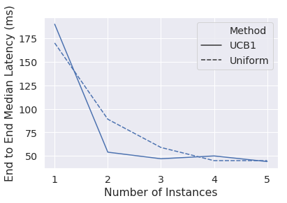
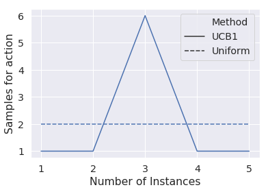
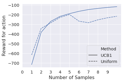
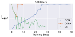
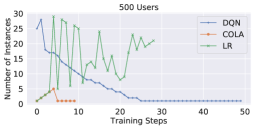
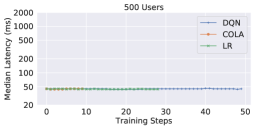
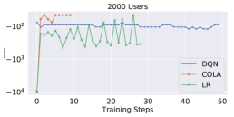
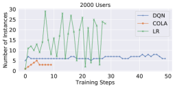
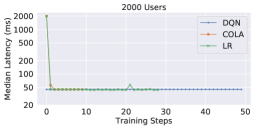
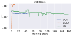
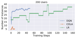
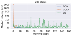
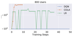
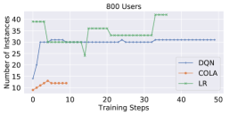
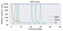
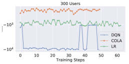
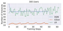
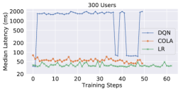
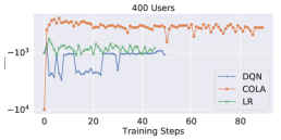
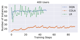
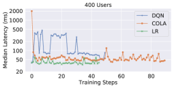
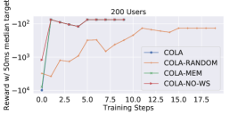
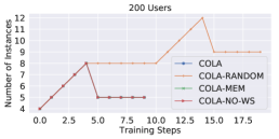
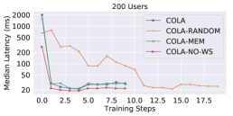
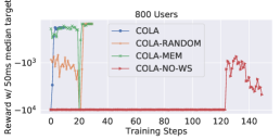
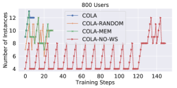
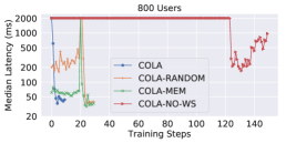
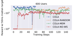
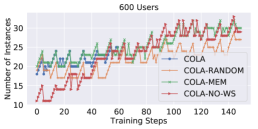
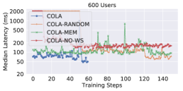
8.16. Open Source Application Modifications
We describe any modifications made to our open source benchmark applications before evaluating on them.
Simple Web Server We add a 40 ms pause to the response on the server side to simulate delay due to application logic.
Online Boutique We modify this microservice application by replacing the load generator service provided with our own external load generator based on Locust (Locust, [n.d.]). When deployed as is, the application contains 12 microservices rather than 11.
Train Ticket We populate the application with usernames and credentials for 10,000 synthetic users. Each connection in our load generator samples a synthetic user uniformly at random, logs in with these credentials and then issues further requests during evaluation. We allow autoscaling on all microservices except the ts-auth-service through which users login.
8.17. Modeling Details
We define the model of our microservice autoscaling problem below.
8.17.1. State
An application consists of different microservice deployments (e.g., database, web server, cache). Each deployment, , has a defined range of number of replicas which may be launched from 1 to . We denote as the replica range for the deployment . We define the state of the cluster, as a vector of number of current deployments for microservices in our application. If we consider the maximum replicas to be for all deployments, the possible states for our microservice application is .
8.17.2. Actions
Our model has the ability to take actions that modify the number of replicas in our cluster for each microservice to any value in its replica range, consequently altering state . The set of all possible actions is simply the set of cluster states, . At any given time a model may choose to change the cluster state to any possible configuration.
8.17.3. Context
We construct a representation of a workload and denote this representation as a context . This context , contains information on the inbound requests to our application and serves to distinguish the workloads an application may observe.
In recent years, standards have been introduced by the OpenTracing (OpenTracing, [n.d.]) and OpenAPI (Foundation, [n.d.]) organizations to define requests into a distinct set of ”operation” names. Roughly speaking, the best practice denotes an operation as a distinct URL without its request parameters. For example, get_account_by_id/id1 and get_account_by_id/id2 both fall under the get_account_by_id operation name.
Several popular logging, monitoring and debugging tools can both propogate and utilize these specified operation names. For example microservice tracing tools (e.g. (Jaeger, [n.d.]), Zipkin (Zipkin, [n.d.]), and DataDog (Datadog, [n.d.]b)) annotate logs of invoked requests with their associated operation name. Monitoring and debugging tools often allow users to filter, process and analyze requests broken down by operation name.
During training and evaluation, we assume that developers have defined distinct operations for their application. We then construct a context vector of length by concatenating the number of requests per operation name. Each element in our context vector is simply the number of requests to our cluster with the operation name .
8.18. Algorithm Hyperparameter Choices
We list the hyperparameters chosen for training learned autoscaling policies across all applications in Table 15.
8.19. Tabular Evaluation Results
8.20. Microservice Application Diagrams
Figure 27 shows the architectures for applications on which we evaluate.
8.21. COLA Training Pseudocode
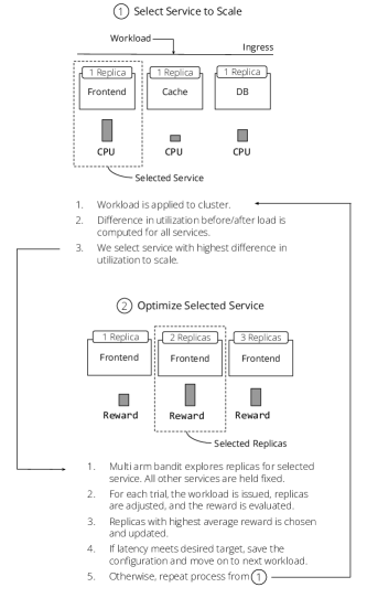
| Variable | Description |
|---|---|
| Set of actions to explore | |
| Latency target (in ms) | |
| Workload | |
| Current weight hyperparameter | |
| Best action in | |
| Latency for best action in |
We provide psuedocode for COLA’s autoscaling training procedure above in Algorithm 1. Also, we document the inputs and outputs to the functions outlined in Algorithm 1 in Tables 14 and 13.
| Variable | Description |
|---|---|
| Workload | |
| Initial cluster state | |
| Latency target (in ms) | |
| Number of iterations | |
| Current weight hyperparameter | |
| Maximum weight hyperparameter | |
| Weight increment | |
| Final cluster state after optimizing | |
| Final latency after optimizing |
| Application | (initial) | Sample Duration | Number of Samples (non COLA) |
|---|---|---|---|
| Simple Web Server | 1/3 | 30 | 200 |
| Book Info. | 1/3 | 25 | 200 |
| Online Boutique. | 1/3 | 60 | 200 |
| Sock Shop. | 1/3 | 80 | 200 |
| Train Ticket | 1/3 | 80 | 250 |
| Users | Policy | Median Latency | Failures/s | VM Instances |
|---|---|---|---|---|
| 300.0 | CPU-30 | 19.4 | 0.00 | 15.00 |
| 300.0 | CPU-70 | 22.5 | 0.24 | 9.37 |
| 300.0 | BO-50ms | 20.1 | 0.00 | 27.58 |
| 300.0 | COLA-50ms | 43.9 | 0.27 | 8.67 |
| 300.0 | DQN-50ms | 2000.0 | 138.36 | 32.00 |
| 300.0 | LR-50ms | 53.6 | 0.00 | 7.00 |
| 400.0 | CPU-30 | 18.9 | 0.00 | 19.00 |
| 400.0 | CPU-70 | 37.5 | 0.00 | 11.00 |
| 400.0 | BO-50ms | 20.4 | 0.00 | 32.00 |
| 400.0 | COLA-50ms | 30.9 | 0.11 | 9.00 |
| 400.0 | DQN-50ms | 2000.0 | 181.96 | 32.00 |
| 400.0 | LR-50ms | 60.6 | 0.00 | 7.00 |
| 700.0 | CPU-30 | 22.0 | 0.41 | 26.40 |
| 700.0 | CPU-70 | 47.6 | 5.57 | 16.10 |
| 700.0 | BO-50ms | 24.3 | 0.00 | 18.00 |
| 700.0 | COLA-50ms | 43.7 | 0.01 | 10.00 |
| 700.0 | DQN-50ms | 2000.0 | 308.87 | 32.00 |
| 700.0 | LR-50ms | 2000.0 | 293.54 | 7.00 |
| 800.0 | CPU-30 | 21.7 | 0.31 | 27.77 |
| 800.0 | CPU-70 | 30.8 | 0.43 | 17.37 |
| 800.0 | BO-50ms | 26.6 | 0.00 | 18.00 |
| 800.0 | COLA-50ms | 37.7 | 0.00 | 10.00 |
| 800.0 | DQN-50ms | 2000.0 | 350.43 | 32.00 |
| 800.0 | LR-50ms | 2000.0 | 357.96 | 7.00 |
| Users | Policy | Median Latency | Failures/s | VM Instances |
|---|---|---|---|---|
| 200.0 | CPU-30 | 11.0 | 0.00 | 25.48 |
| 200.0 | CPU-70 | 18.4 | 0.00 | 15.65 |
| 200.0 | BO-50ms | 43.7 | 0.13 | 34.97 |
| 200.0 | COLA-50ms | 14.3 | 0.04 | 15.00 |
| 200.0 | DQN-50ms | 9.0 | 0.00 | 48.00 |
| 200.0 | LR-50ms | 43.7 | 0.00 | 14.00 |
| 300.0 | CPU-30 | 11.1 | 0.13 | 29.57 |
| 300.0 | CPU-70 | 23.9 | 0.02 | 15.00 |
| 300.0 | BO-50ms | 37.9 | 42.61 | 29.27 |
| 300.0 | COLA-50ms | 26.0 | 0.18 | 15.00 |
| 300.0 | DQN-50ms | 9.1 | 0.00 | 48.00 |
| 300.0 | LR-50ms | 59.5 | 0.01 | 14.00 |
| 400.0 | CPU-30 | 10.5 | 10.56 | 32.03 |
| 400.0 | CPU-70 | 17.4 | 0.00 | 16.00 |
| 400.0 | BO-50ms | 193.2 | 25.56 | 23.67 |
| 400.0 | COLA-50ms | 33.8 | 0.46 | 15.00 |
| 400.0 | DQN-50ms | 9.3 | 0.00 | 48.00 |
| 400.0 | LR-50ms | 32.9 | 0.00 | 15.00 |
| 500.0 | CPU-30 | 11.5 | 0.10 | 41.07 |
| 500.0 | CPU-70 | 23.3 | 1.54 | 18.65 |
| 500.0 | BO-50ms | 409.4 | 93.34 | 23.72 |
| 500.0 | COLA-50ms | 43.0 | 0.92 | 15.00 |
| 500.0 | DQN-50ms | 9.5 | 0.00 | 48.00 |
| 500.0 | LR-50ms | 44.5 | 0.00 | 15.00 |
| Users | Policy | Median Latency | Failures/s | VM Instances |
|---|---|---|---|---|
| 500.0 | CPU-30 | 38.6 | 0.10 | 45.55 |
| 500.0 | CPU-70 | 58.1 | 0.48 | 21.00 |
| 500.0 | BO-50ms | 842.4 | 94.62 | 44.88 |
| 500.0 | COLA-50ms | 50.0 | 0.61 | 24.70 |
| 500.0 | DQN-50ms | 2000.0 | 209.09 | 55.00 |
| 500.0 | LR-50ms | 562.0 | 0.75 | 19.22 |
| 600.0 | CPU-30 | 38.7 | 0.10 | 51.3 |
| 600.0 | CPU-70 | 59.3 | 0.17 | 22.85 |
| 600.0 | BO-50ms | 443.7 | 59.16 | 43.97 |
| 600.0 | COLA-50ms | 47.9 | 0.23 | 27.00 |
| 600.0 | DQN-50ms | 2000.0 | 244.25 | 54.25 |
| 600.0 | LR-50ms | 1171.0 | 49.26 | 19.00 |
| 700.0 | CPU-30 | 39.1 | 0.14 | 58.07 |
| 700.0 | CPU-70 | 61.0 | 0.26 | 24.80 |
| 700.0 | BO-50ms | 1837.0 | 247.64 | 41.28 |
| 700.0 | COLA-50ms | 51.3 | 0.52 | 26.65 |
| 700.0 | DQN-50ms | 2000.0 | 275.57 | 55.00 |
| 700.0 | LR-50ms | 1970.0 | 156.16 | 19.00 |
| 800.0 | CPU-30 | 43.6 | 0.36 | 67.42 |
| 800.0 | CPU-70 | 73.3 | 1.07 | 27.23 |
| 800.0 | BO-50ms | 550.7 | 92.13 | 46.47 |
| 800.0 | COLA-50ms | 54.0 | 1.05 | 29.38 |
| 800.0 | DQN-50ms | 2000.0 | 324.64 | 55.00 |
| 800.0 | LR-50ms | 2000.0 | 299.95 | 19.00 |
| Users | Policy | Median Latency | Failures/s | VM Instances |
|---|---|---|---|---|
| 250.0 | CPU-30 | 45.9 | 0.05 | 103.07 |
| 250.0 | CPU-70 | 50.4 | 0.02 | 78.60 |
| 250.0 | BO-50ms | 60.8 | 2.19 | 275.80 |
| 250.0 | COLA-50ms | 47.5 | 0.00 | 77.00 |
| 250.0 | DQN-50ms | 51.6 | 0.00 | 352.80 |
| 250.0 | LR-50ms | 219.6 | 20.63 | 111.22 |
| 500.0 | CPU-30 | 47.0 | 0.38 | 119.67 |
| 500.0 | CPU-70 | 56.6 | 7.03 | 84.68 |
| 500.0 | BO-50ms | 1311.0 | 135.49 | 279.93 |
| 500.0 | COLA-50ms | 49.8 | 0.07 | 82.00 |
| 500.0 | DQN-50ms | 92.7 | 0.00 | 353.00 |
| 500.0 | LR-50ms | 67.9 | 1.05 | 115.52 |
| 600.0 | CPU-30 | 47.3 | 0.55 | 130.03 |
| 600.0 | CPU-70 | 68.4 | 13.92 | 84.50 |
| 600.0 | BO-50ms | 370.3 | 60.31 | 269.93 |
| 600.0 | COLA-50ms | 56.3 | 10.11 | 84.43 |
| 600.0 | DQN-50ms | 922.0 | 84.60 | 353.00 |
| 600.0 | LR-50ms | 1328.0 | 184.86 | 109.20 |
| Users | Policy | 90%ile Latency | Failures/s | VM Instances |
|---|---|---|---|---|
| 250.0 | CPU-30 | 69.8 | 0.04 | 97.30 |
| 250.0 | CPU-70 | 160.4 | 0.03 | 76.30 |
| 250.0 | COLA-100ms | 83.4 | 0.06 | 77.00 |
| 400.0 | CPU-30 | 74.6 | 0.04 | 106.10 |
| 400.0 | CPU-70 | 563.2 | 5.60 | 78.87 |
| 400.0 | COLA-100ms | 107.0 | 0.00 | 79.00 |
| 500.0 | CPU-30 | 73.8 | 0.22 | 112.97 |
| 500.0 | CPU-70 | 109.0 | 0.10 | 83.23 |
| 500.0 | COLA-100ms | 471.0 | 6.62 | 87.98 |
| 600.0 | CPU-30 | 77.4 | 0.26 | 115.87 |
| 600.0 | CPU-70 | 180.0 | 0.03 | 84.27 |
| 600.0 | COLA-100ms | 91.4 | 0.00 | 89.00 |
| Users | Policy | 90%ile Latency | Failures/s | VM Instances |
|---|---|---|---|---|
| 600.0 | CPU-30 | 74.2 | 0.08 | 51.10 |
| 600.0 | CPU-70 | 158.0 | 0.22 | 23.00 |
| 600.0 | COLA-100ms | 95.8 | 0.03 | 33.57 |
| 800.0 | CPU-30 | 77.6 | 0.02 | 69.90 |
| 800.0 | CPU-70 | 334.0 | 1.07 | 28.30 |
| 800.0 | COLA-100ms | 136.0 | 0.31 | 33.30 |
| Users | Policy | Median Latency | Failures/s | VM Instances |
|---|---|---|---|---|
| In Sample | CPU-30 | 42.3 | 0.03 | 34.62 |
| In Sample | CPU-70 | 57.7 | 0.41 | 15.97 |
| In Sample | BO-50ms | 1050.0 | 71.78 | 35.28 |
| In Sample | COLA-50ms | 52.3 | 0.25 | 18.38 |
| In Sample | DQN-50ms | 1182.0 | 59.82 | 52.51 |
| In Sample | LR-50ms | 65.0 | 0.32 | 22.63 |
| Out of Sample | CPU-30 | 38.6 | 0.04 | 28.77 |
| Out of Sample | CPU-70 | 53.3 | 0.38 | 15.21 |
| Out of Sample | BO-50ms | 715.3 | 42.76 | 47.73 |
| Out of Sample | COLA-50ms | 45.6 | 0.15 | 17.37 |
| Out of Sample | DQN-50ms | 885.3 | 34.96 | 52.73 |
| Out of Sample | LR-50ms | 58.7 | 0.61 | 21.57 |
| Users | Policy | Median Latency | Failures/s | VM Instances |
|---|---|---|---|---|
| In Sample | CPU-30 | 21.7 | 0.00 | 10.47 |
| In Sample | CPU-70 | 46.7 | 9.66 | 6.18 |
| In Sample | BO-50ms | 18.0 | 0.00 | 25.94 |
| In Sample | COLA-50ms | 39.3 | 9.62 | 6.41 |
| In Sample | DQN-50ms | 1430.0 | 115.43 | 31.94 |
| In Sample | LR-50ms | 21.3 | 0.68 | 11.88 |
| Out of Sample | CPU-30 | 21.7 | 0.02 | 11.19 |
| Out of Sample | CPU-70 | 26.3 | 0.00 | 5.84 |
| Out of Sample | BO-50ms | 19.3 | 3.90 | 30.00 |
| Out of Sample | COLA-50ms | 24.3 | 0.00 | 6.27 |
| Out of Sample | DQN-50ms | 1473.3 | 123.81 | 31.40 |
| Out of Sample | LR-50ms | 21.3 | 0.00 | 12.65 |
| Users | Policy | Median Latency | Failures/s | VM Instances |
|---|---|---|---|---|
| In Sample | CPU-30 | 45.0 | 0.02 | 8.44 |
| In Sample | CPU-70 | 54.0 | 67.29 | 3.08 |
| In Sample | BO-50ms | 44.0 | 0.00 | 14.79 |
| In Sample | COLA-50ms | 46.0 | 0.00 | 1.98 |
| In Sample | DQN-50ms | 44.0 | 0.00 | 6.00 |
| In Sample | LR-50ms | 44.0 | 0.00 | 6.71 |
| Out of Sample | CPU-30 | 45.0 | 0.00 | 8.24 |
| Out of Sample | CPU-70 | 45.7 | 0.00 | 3.30 |
| Out of Sample | BO-50ms | 44.0 | 0.10 | 18.31 |
| Out of Sample | COLA-50ms | 45.3 | 0.00 | 2.24 |
| Out of Sample | DQN-50ms | 44.0 | 0.00 | 7.63 |
| Out of Sample | LR-50ms | 44.0 | 0.00 | 6.87 |
| Users | Policy | Median Latency | Failures/s | VM Instances |
|---|---|---|---|---|
| In Sample | CPU-30 | 50.0 | 0.00 | 74.53 |
| In Sample | CPU-70 | 49.3 | 0.00 | 73.16 |
| In Sample | BO-50ms | 1343.3 | 184.94 | 290.95 |
| In Sample | COLA-50ms | 92.3 | 62.31 | 78.62 |
| In Sample | DQN-50ms | 1900.0 | 183.13 | 350.69 |
| In Sample | LR-50ms | 853.3 | 149.59 | 110.86 |
| Out of Sample | CPU-30 | 57.7 | 11.11 | 131.62 |
| Out of Sample | CPU-70 | 166.3 | 78.28 | 83.07 |
| Out of Sample | BO-50ms | 718.3 | 127.76 | 270.43 |
| Out of Sample | COLA-50ms | 48.0 | 0.78 | 73.00 |
| Out of Sample | DQN-50ms | 48.0 | 45.23 | 354.20 |
| Out of Sample | LR-50ms | 56.0 | 0.84 | 102.50 |
| Users | Policy | Median Latency | Failures/s | VM Instances |
|---|---|---|---|---|
| In Sample | CPU-30 | 11.3 | 6.61 | 28.37 |
| In Sample | CPU-70 | 26.3 | 9.70 | 17.42 |
| In Sample | BO-50ms | 9.7 | 50.97 | 28.23 |
| In Sample | COLA-50ms | 15.3 | 0.00 | 15.70 |
| In Sample | DQN-50ms | 10.0 | 0.00 | 50.00 |
| In Sample | LR-50ms | 306.3 | 15.43 | 14.00 |
| Out of Sample | CPU-30 | 10.7 | 8.22 | 30.06 |
| Out of Sample | CPU-70 | 20.0 | 0.01 | 15.64 |
| Out of Sample | BO-50ms | 23.3 | 60.32 | 23.38 |
| Out of Sample | COLA-50ms | 25.7 | 0.00 | 15.00 |
| Out of Sample | DQN-50ms | 9.7 | 0.01 | 47.95 |
| Out of Sample | LR-50ms | 148.0 | 3.68 | 14.28 |
| Policy | Median Latency | Failures/s | VM Instances |
|---|---|---|---|
| CPU-30 | 12.5 | 4.01 | 26.44 |
| CPU-70 | 24.3 | 8.79 | 15.00 |
| BO-50ms | 21.0 | 74.85 | 23.25 |
| COLA-50ms | 41.0 | 6.35 | 14.10 |
| LR-50ms | 49.3 | 7.75 | 14.47 |
| Users | Policy | Median Latency | Failures/s | VM Instances |
|---|---|---|---|---|
| 300.0 | CPU-30 | 39.8 | 3.77 | 53.00 |
| 300.0 | CPU-70 | 55.4 | 6.09 | 23.43 |
| 300.0 | COLA-50ms | 49.2 | 6.93 | 29.00 |
| Users | Policy | Median Latency | Failures/s | VM Instances |
|---|---|---|---|---|
| 100 | CPU-10 | 19.7 | 0.02 | 20.15 |
| 100 | CPU-30 | 17.1 | 0.00 | 13.07 |
| 100 | CPU-50 | 19.0 | 0.00 | 8.42 |
| 100 | CPU-70 | 20.3 | 0.05 | 8.32 |
| 100 | CPU-90 | 54.7 | 0.00 | 4.00 |
| 100 | COLA-50ms | 24.8 | 0.00 | 5.00 |
| 250 | CPU-10 | 19.3 | 0.00 | 33.47 |
| 250 | CPU-30 | 19.5 | 0.00 | 8.58 |
| 250 | CPU-50 | 24.6 | 0.00 | 6.10 |
| 250 | CPU-70 | 40.7 | 0.00 | 5.17 |
| 250 | CPU-90 | 39.9 | 0.00 | 5.00 |
| 250 | COLA-50ms | 25.2 | 0.00 | 6.00 |
| 700 | CPU-10 | 19.8 | 0.00 | 33.73 |
| 700 | CPU-30 | 23.7 | 0.00 | 17.88 |
| 700 | CPU-50 | 30.8 | 0.00 | 11.83 |
| 700 | CPU-70 | 200.5 | 26.46 | 11.72 |
| 700 | CPU-90 | 205.7 | 111.99 | 12.48 |
| 700 | COLA-50ms | 30.6 | 0.00 | 10.00 |
| 850 | CPU-10 | 21.7 | 0.43 | 36.64 |
| 850 | CPU-30 | 28.3 | 8.26 | 22.07 |
| 850 | CPU-50 | 32.6 | 10.77 | 16.62 |
| 850 | CPU-70 | 43.7 | 0.01 | 11.32 |
| 850 | CPU-90 | 43.9 | 3.41 | 10.58 |
| 850 | COLA-50ms | 35.3 | 0.00 | 10.00 |
| 1100 | CPU-10 | 23.6 | 0.36 | 39.25 |
| 1100 | CPU-30 | 24.7 | 0.47 | 24.65 |
| 1100 | CPU-50 | 37.8 | 0.92 | 20.23 |
| 1100 | CPU-70 | 1055.6 | 247.04 | 12.63 |
| 1100 | CPU-90 | 80.4 | 0.02 | 9.8 |
| 1100 | COLA-50ms | 42.7 | 0.00 | 11.00 |
| 1250 | CPU-10 | 25.7 | 0.00 | 41.50 |
| 1250 | CPU-30 | 25.6 | 0.04 | 23.90 |
| 1250 | CPU-50 | 82.1 | 1.77 | 20.10 |
| 1250 | CPU-70 | 75.2 | 0.65 | 15.38 |
| 1250 | CPU-90 | 652.0 | 73.70 | 11.72 |
| 1250 | COLA-50ms | 46.6 | 0.00 | 12.00 |
| Users | Policy | Median Latency | Failures/s | Number of Pods | VM Instances |
|---|---|---|---|---|---|
| 500 | CPU-30 | 45.0 | 0.0 | 5.266667 | 5.833333 |
| 500 | CPU-70 | 46.2 | 0.0 | 2.0 | 1.0 |
| 500 | COLA-50ms | 44.0 | 0.0 | 2.0 | 1.0 |
| 1000 | CPU-30 | 45.0 | 0.0 | 10.0 | 5.0 |
| 1000 | CPU-70 | 46.0 | 0.0 | 4.0 | 2.0 |
| 1000 | COLA-50ms | 45.0 | 0.0 | 3.0 | 2.0 |
| 2000 | CPU-30 | 45.0 | 0.0 | 18.0 | 9.0 |
| 2000 | CPU-70 | 46.0 | 0.0 | 7.0 | 4.0 |
| 2000 | COLA-50ms | 46.0 | 0.0 | 5.0 | 3.5 |
| Users | Policy | Median Latency | Failures/s | Number of Pods | VM Instances |
|---|---|---|---|---|---|
| 500 | CPU-30 | 44.0 | 0.0 | 5.0 | 2.6 |
| 500 | CPU-70 | 44.0 | 0.0 | 2.0 | 1.0 |
| 500 | COLA-50ms | 44.6 | 0.0 | 2.0 | 1.0 |
| 1000 | CPU-30 | 44.0 | 0.0 | 9.0 | 2.0 |
| 1000 | CPU-70 | 44.2 | 0.0 | 4.0 | 1.0 |
| 1000 | COLA-50ms | 45.0 | 0.0 | 3.0 | 1.0 |
| 2000 | CPU-30 | 44.0 | 0.0 | 19.0 | 4.0 |
| 2000 | CPU-70 | 45.0 | 0.0 | 7.0 | 2.0 |
| 2000 | COLA-50ms | 45.0 | 0.0 | 6.0 | 2.0 |
| Users | Policy | Median Latency | Failures/s | Number of Pods | VM Instances |
|---|---|---|---|---|---|
| 200 | CPU-30 | 20.6 | 0.00 | 12.0 | 11.0 |
| 200 | CPU-70 | 26.2 | 0.00 | 7.0 | 4.0 |
| 200 | COLA-50ms | 35.6 | 0.00 | 6.0 | 3.5 |
| 300 | CPU-30 | 22.0 | 0.0 | 18.6 | 19.9 |
| 300 | CPU-70 | 43.0 | 0.0 | 8.0 | 4.0 |
| 300 | COLA-50ms | 37.2 | 0.0 | 8.0 | 4.0 |
| Users | Policy | Median Latency | Failures/s | Number of Pods | VM Instances |
|---|---|---|---|---|---|
| 200 | CPU-30 | 18.6 | 0.0 | 13.4 | 8.0 |
| 200 | CPU-70 | 25.2 | 0.0 | 7.0 | 2.0 |
| 200 | COLA-50ms | 22.8 | 0.0 | 6.0 | 2.0 |
| 300 | CPU-30 | 19.4 | 0.0 | 16.0 | 5.0 |
| 300 | CPU-70 | 30.4 | 0.0 | 9.0 | 2.0 |
| 300 | COLA-50ms | 46.6 | 0.0 | 7.0 | 2.0 |
| Users | Policy | Median Latency | Failures/s | Number of Pods | VM Instances |
|---|---|---|---|---|---|
| 100 | CPU-30 | 54.6 | 0.00 | 22.0 | 11.0 |
| 100 | CPU-70 | 69.6 | 0.17 | 13.0 | 7.0 |
| 100 | COLA-50ms | 49.4 | 0.10 | 20.0 | 9.0 |
| 150 | CPU-30 | 57.6 | 0.28 | 28.0 | 14.0 |
| 150 | CPU-70 | 88.8 | 0.42 | 14.0 | 7.0 |
| 150 | COLA-50ms | 52.0 | 0.02 | 22.0 | 9.0 |
| Users | Policy | Median Latency | Failures/s | Number of Pods | VM Instances |
|---|---|---|---|---|---|
| 100 | CPU-30 | 47.6 | 0.41 | 23.06 | 5.0 |
| 100 | CPU-70 | 61.4 | 0.63 | 13.63 | 3.0 |
| 100 | COLA-50ms | 48.4 | 0.19 | 15.00 | 3.5 |
| 150 | CPU-30 | 46.4 | 0.37 | 30.6 | 6.57 |
| 150 | CPU-70 | 53.6 | 0.97 | 17.0 | 4.00 |
| 150 | COLA-50ms | 47.0 | 0.60 | 19.0 | 4.50 |
| Users | Policy | Median Latency | Failures/s | Number of Pods |
|---|---|---|---|---|
| 200 | CPU-30 | 26.8 | 0.93 | 10.73 |
| 200 | CPU-70 | 2000.0 | 92.76 | 6.95 |
| 200 | COLA-50ms | 27.7 | 8.90 | 9.13 |
| 300 | CPU-30 | 26.6 | 0.0 | 14.0 |
| 300 | CPU-70 | 2000.0 | 137.77 | 7.8 |
| 300 | COLA-50ms | 29.1 | 0.0 | 10.0 |
| 400 | CPU-30 | 27.1 | 0.0 | 16.0 |
| 400 | CPU-70 | 2000.0 | 181.89 | 8.55 |
| 400 | COLA-50ms | 28.3 | 0.545 | 13.0 |
| 500 | CPU-30 | 42.0 | 20.23 | 28.9 |
| 500 | CPU-70 | 2000.0 | 224.39 | 9.45 |
| 500 | COLA-50ms | 39.0 | 0.00 | 13.0 |
| Users | Policy | Median Latency | Failures/s | Number of Pods |
|---|---|---|---|---|
| 100 | CPU-30 | 48.0 | 0.12 | 18.85 |
| 100 | CPU-70 | 180.0 | 0.24 | 11.0 |
| 100 | COLA-50ms | 46.3 | 0.00 | 14.18 |
| 150 | CPU-30 | 47.1 | 0.00 | 21.52 |
| 150 | CPU-70 | 132.4 | 0.24 | 12.0 |
| 150 | COLA-50ms | 47.3 | 0.14 | 17.87 |
| 200 | CPU-30 | 50.1 | 0.06 | 25.02 |
| 200 | CPU-70 | 200.0 | 0.38 | 12.97 |
| 200 | COLA-50ms | 53.9 | 0.56 | 18.0 |
| Users | Policy | Median Latency | Failures/s | Number of Pods |
|---|---|---|---|---|
| 100 | CPU-30 | 39.0 | 0.0 | 73.0 |
| 100 | CPU-70 | 37.8 | 14.97 | 73.0 |
| 100 | COLA-50ms | 39.8 | 0.53 | 73.23 |
| 200 | CPU-30 | 43.8 | 0.00 | 82.53 |
| 200 | CPU-70 | 38.4 | 29.44 | 73.0 |
| 200 | COLA-50ms | 37.0 | 0.0 | 75.0 |
| 350 | CPU-30 | 49.4 | 1.42 | 92.77 |
| 350 | CPU-70 | 40.2 | 50.32 | 74.3 |
| 350 | COLA-50ms | 39.6 | 0.0 | 76.0 |
