Analysis and Control of Input-Affine Dynamical Systems
using Infinite-Dimensional Robust Counterparts

Jared Miller1,2, Mario Sznaier2 1J. Miller is with the Automatic Control Laboratory (IfA), Department of Information Technology and Electrical Engineering (D-ITET), ETH Zürich, Phisykstrasse 3, 8092, Zürich, Switzerland (e-mail: jarmiller@control.ee.ethz.ch).2J. Miller and M. Sznaier are with the Robust Systems Lab, ECE Department, Northeastern University, Boston, MA 02115. (e-mails: msznaier@coe.neu.edu). J. Miller and M. Sznaier were partially supported by National Science Foundation (NSF) grants CNS–1646121, CMMI–1638234, ECCS–1808381 and CNS–2038493, and Air Force Office of Scientific Research (AFOSR) grant FA9550-19-1-0005. J. Miller was partially supported by the Swiss National Science Foundation Grant 200021_178890 (NCCR: Automation), and by the Chateaubriand Fellowship of the Office for Science & Technology of the Embassy of France in the United States.
Abstract

Input-affine dynamical systems often arise in control and modeling scenarios, such as the data-driven case when state-derivative observations are recorded under bounded noise. Common tasks in system analysis and control include optimal control, peak estimation, reachable set estimation, and maximum control invariant set estimation. Existing work poses these types of problems as infinite-dimensional linear programs in auxiliary functions with sum-of-squares tightenings. The bottleneck in most of these programs is the Lie derivative nonnegativity constraint posed over the time-state-control set. Decomposition techniques to improve tractability by eliminating the control variables include vertex decompositions (switching), or facial decompositions in the case where the polytopic set is a scaled box. This work extends the box-facial decomposition technique to allow for a robust-counterpart decomposition of semidefinite representable sets (e.g. polytopes, ellipsoids, and projections of spectahedra). These robust counterparts are proven to be equivalent to the original Lie constraint under mild compactness and regularity constraints. Efficacy is demonstrated under peak/distance/reachable set data-driven analysis problems and Region of Attraction maximizing control.

1 Introduction

This paper will focus on analysis of an input-affine and continuous-time dynamical system under an input process w(t)𝑤𝑡w(t) with

x˙(t)=f(t,x(t),w(t))=f0(t,x)+=1Lw(t)f(t,x),˙𝑥𝑡𝑓𝑡𝑥𝑡𝑤𝑡subscript𝑓0𝑡𝑥superscriptsubscript1𝐿subscript𝑤𝑡subscript𝑓𝑡𝑥\dot{x}(t)=f(t,x(t),w(t))=f_{0}(t,x)+\textstyle\sum_{\ell=1}^{L}w_{\ell}(t)f_{\ell}(t,x), (1)

in which the state xXn𝑥𝑋superscript𝑛x\in X\subset\mathbb{R}^{n} and the input wWL𝑤𝑊superscript𝐿w\in W\subset\mathbb{R}^{L} are assumed to lie in compact sets. The time horizon t[0,T]𝑡0𝑇t\in[0,T] is finite for convergence purposes. It is further required that the set W𝑊W is an L𝐿L-dimensional compact Semidefinite Representable (SDR) set (a projection of a spectahedron) with non-empty interior [1].

\@firstupper\@iaci

SDR SDR set could arise from a sequence of observations of x˙(t)˙𝑥𝑡\dot{x}(t) as corrupted by bounded noise. An example of such \@iaciSDR SDR set W𝑊W is the L𝐿L-dimensional polytope described by m𝑚m constraints (up to m𝑚m faces), which may be expressed as

W𝑊\displaystyle W ={wAwb}absentconditional-set𝑤𝐴𝑤𝑏\displaystyle=\{w\mid Aw\leq b\} Am×L,bm.formulae-sequence𝐴superscript𝑚𝐿𝑏superscript𝑚\displaystyle A\in\mathbb{R}^{m\times L},\ b\in\mathbb{R}^{m}. (2)

Letting x0X0subscript𝑥0subscript𝑋0x_{0}\in X_{0} be an initial condition and w(t)𝑤𝑡w(t) be a control with w(t)Wt[0,T]𝑤𝑡𝑊for-all𝑡0𝑇w(t)\in W\ \forall t\in[0,T] and T𝑇T finite, the state obtained by following dynamics in (1) is

x(t)=x(tx0,w()).𝑥𝑡𝑥conditional𝑡subscript𝑥0𝑤x(t)=x(t\mid x_{0},w(\cdot)). (3)

The process w(t)𝑤𝑡w(t) is well-defined for each value of t[0,T]𝑡0𝑇t\in[0,T], but is not required to be continuous.

The problem instances that will be addressed in this paper are peak estimation, distance estimation, reachable set estimation, and Region of Attraction (ROA) maximization. Each problem instance may be cast as an infinite-dimensional Linear Program (LP) and approximated through the moment- Sum of Squares (SOS) hierarchy. They each have a Lie derivative nonnegativity constraint that usually induces the largest PSD matrix by numerical solvers. Such a constraint may be split using infinite-dimensional robust counterparts [2] into smaller Positive Semidefinite (PSD) matrix constraints using convex duality [3] and a theorem of alternatives [4]. Decomposition of SDR sets W𝑊W move beyond the previously considered box cases in [5] [6] and polytope case in [7].

Peak estimation finds an initial condition x0subscript𝑥0x_{0} and input w𝑤w that maximizes the instantaneous value of a state function p(x(t))𝑝𝑥𝑡p(x(t)) along a trajectory [8]. Distance estimation is a variation of peak estimation that finds the distance of closest approach between points along trajectories x(tx0,w)𝑥conditional𝑡subscript𝑥0𝑤x(t\mid x_{0},w) and an unsafe set Xusubscript𝑋𝑢X_{u} [9]. Reachable set estimation identifies the set of points XTsubscript𝑋𝑇X_{T} such that there exists a pair x0,wsubscript𝑥0𝑤x_{0},w where x(Tx0,w)XT𝑥conditional𝑇subscript𝑥0𝑤subscript𝑋𝑇x(T\mid x_{0},w)\in X_{T} [10]. Peak and reachable set estimation under input-affine and SDR constraints may arise from the data-driven setting where state-derivative observations 𝒟={(tk,xk,yk)}k=1Ns𝒟superscriptsubscriptsubscript𝑡𝑘subscript𝑥𝑘subscript𝑦𝑘𝑘1subscript𝑁𝑠\mathcal{D}=\{(t_{k},x_{k},{y}_{k})\}_{k=1}^{N_{s}} are available subject to an L,subscript𝐿L_{\infty}, L2subscript𝐿2L_{2}, or semidefinite-bounded noise process η𝜂\eta (y(tk)x˙(tk)+ηkapproaches-limit𝑦subscript𝑡𝑘˙𝑥subscript𝑡𝑘subscript𝜂𝑘y(t_{k})\doteq\dot{x}(t_{k})+\eta_{k}). As an example, Lsubscript𝐿L_{\infty}-bounded noise could arise from propagating finite-difference errors from when estimate x˙˙𝑥\dot{x}.

Basin/ROA estimation problems based on Backwards Reachable Set (BRS) approaches have similar principles as forward Reachable set estimation problems. [11]. ROA maximization chooses a control scheme w(t)𝑤𝑡w(t) that optimizes the volume of the set X0subscript𝑋0X_{0} such that initial conditions x0X0subscript𝑥0subscript𝑋0x_{0}\in X_{0} will land in a goal set XTsubscript𝑋𝑇X_{T}.

Application of infinite-dimensional LPs to problems in control theory began with optimal control in [12]. Solution methods for these infinite-dimensional LPs include gridded discretization and the moment-SOS hierarchy of Semidefinite Programs in [13]. Peak estimation LPs were solved by discretization in [8] and through SOS methods in [14], with moment-based optima recovery in [15]. Peak estimation under uncertainty was treated in [16], and this work will use the input-affine and SDR structure W𝑊W to generate simpler SDPs.

Reachable set estimation using LPs occurs from outside in [17] and from inside in [18]. SDPs associated with the moment-SOS hierarchy will produce polynomial sublevel sets that converge in volume to the true reachable set as the polynomial degree increases (under mild conditions, and outside a set of measures zero). Controllers may be formulated to maximize the BRS, in which the volume of the set of initial conditions X0subscript𝑋0X_{0} that can be steered towards a target set XTsubscript𝑋𝑇X_{T} is maximized [19]. Other approaches towards reachable set estimation of nonlinear systems includes ellipsoidal methods [20], polytopes [21], and interval methods using mixed monotonicity [22]. Infinite-dimensional LPs have also been applied to region of attraction estimation and backwards reachable set maximizing control [17]. We note that recent work in [23] involves data-driven estimation of the Lie derivative/infinitesimal generator for use in auxiliary function programs (e.g. time-averages).

The power of infinite-dimensional robust counterparts in reducing the dimensionality of PSD matrices can be demonstrated on a peak estimation task in dimension n=2𝑛2n=2, possessing disturbance-affine cubic polynomial dynamics (discussed further in Section 7.2). The uncertainty process w(t)𝑤𝑡w(t) is restricted to an polytope W𝑊W with L=10𝐿10L=10 dimensions, Nf=33subscript𝑁𝑓33N_{f}=33 faces, and Nv=7534subscript𝑁𝑣7534N_{v}=7534 vertices. The PSD constraint of maximal size involved in a degree d=4𝑑4d=4 SOS tightening of a peak estimation problem shrinks from 8568 (prior work in [16]) down to 56 (current work) after application of the infinite-dimensional robust counterpart to eliminate the uncertainty variables. Performing a size-8568 dense PSD constraint in solvers such as Mosek or Sedumi is intractable. Applying a vertex decomposition would require that Nv=7534subscript𝑁𝑣7534N_{v}=7534 PSD constraints of size 56 hold. In contrast, the robust counterpart in introduced in this work needs only Nf+1=34subscript𝑁𝑓134N_{f}+1=34 PSD constraints of size 56.

The contributions of this paper are,

  • Formulation of infinite-dimensional robust counterparts with respect to SDR sets along with conditions for their nonconservatism

  • Evaluation of robust counterparts for Lie constraints in input-affine nonlinear systems analysis with SDR input sets W𝑊W

  • Quantification of SDP computational complexity reduction as compared to original programs

  • Demonstration of robust counterparts on peak and reachable set problems

Portions of this paper were presented at the 10th IFAC Symposium on Robust Control Design (ROCOND 2022) [7]. Additional content present in this paper beyond the conference version includes:

  • Generalization of facial (polytopes) decompositions to robust counterparts of SDR sets

  • Distance and (Backwards) Reachable set estimation problems

  • Robustification of discrete-time dynamics

  • Additional examples

  • Proofs of lower semicontinuity, polynomial approximability, and nonconservatism

  • Duality with measure programs and controller recovery

This paper has the following layout: Section 2 provides an overview of preliminaries including notation, the analysis and control problems, robust counterparts, and SOS theory. Section 3 splits the Lie derivative constraint over the SDR uncertainty W𝑊W through the use of an parameterized robust counterpart. Section 4 details SOS programs for the robust counterparts. Section 5 applies parameterized robust counterparts to simplify problems with discrete-time dynamics. Section 6 reviews background of the polyhedral structure of consistency constraints induced by model structures and Lsubscript𝐿L_{\infty}-bounded noise processes. Section 7 presents examples of robust counterparts acting on all four problems. Section 8 concludes the paper.

2 Preliminaries

2.1 Acronyms/Initialisms

BSA
Basic Semialgebraic
BRS
Backwards Reachable Set
LMI
Linear Matrix Inequality
LP
Linear Program
OCP
Optimal Control Problem
PD
Positive Definite
PMI
Polynomial Matrix Inequality
PSD
Positive Semidefinite
ROA
Region of Attraction
SOC
Second Order Cone
SDP
Semidefinite Program
SDR
Semidefinite Representable
SIR
Susceptible, Infected, Removed
SOS
Sum of Squares
TV
Total Variation
WSOS
Weighted Sum of Squares

2.2 Notation

The set of real numbers and its n𝑛n-dimensional Euclidean space are \mathbb{R} and nsuperscript𝑛\mathbb{R}^{n}. The notation 𝟎0\mathbf{0} and 𝟏1\mathbf{1} will denote vectors of all zeros and all ones respectively. The set of natural numbers is \mathbb{N}, and the subset of natural numbers between 111 and n𝑛n is 1..n1..n. An element-wise partial ordering xy𝑥𝑦x\geq y exists between x,yn𝑥𝑦superscript𝑛x,y\in\mathbb{R}^{n} if xiyisubscript𝑥𝑖subscript𝑦𝑖x_{i}\geq y_{i} for each coordinate i=1..ni=1..n. All vectors in the nonnegative orthant x0nn𝑥subscriptsuperscript𝑛absent0superscript𝑛x\in\mathbb{R}^{n}_{\geq 0}\subset\mathbb{R}^{n} satisfy x𝟎𝑥0x\geq\mathbf{0}. The positive orthant is >0nsubscriptsuperscript𝑛absent0\mathbb{R}^{n}_{>0}. The inner product between two vectors x,yn𝑥𝑦superscript𝑛x,y\in\mathbb{R}^{n} may be written as xy=xTy=ixiyi𝑥𝑦superscript𝑥𝑇𝑦subscript𝑖subscript𝑥𝑖subscript𝑦𝑖x\cdot y=x^{T}y=\sum_{i}x_{i}y_{i}.

The set of m×n𝑚𝑛m\times n matrices with real values is m×nsuperscript𝑚𝑛\mathbb{R}^{m\times n}. The set of symmetric matrices 𝕊nsuperscript𝕊𝑛\mathbb{S}^{n} satisfy Q=QT,Qn×nformulae-sequence𝑄superscript𝑄𝑇𝑄superscript𝑛𝑛Q=Q^{T},Q\in\mathbb{R}^{n\times n}. The set of PSD matrices is 𝕊+nsuperscriptsubscript𝕊𝑛\mathbb{S}_{+}^{n} (Q0)succeeds-or-equals𝑄0(Q\succeq 0), and the set of Positive Definite (PD) matrices is 𝕊++nsuperscriptsubscript𝕊absent𝑛\mathbb{S}_{++}^{n} (Q0)succeeds𝑄0(Q\succ 0). The duality paring between two symmetric matrices A,B𝕊n𝐴𝐵superscript𝕊𝑛A,B\in\mathbb{S}^{n} is A,B𝕊n=ijAijBij.subscript𝐴𝐵superscript𝕊𝑛subscript𝑖𝑗subscript𝐴𝑖𝑗subscript𝐵𝑖𝑗\langle A,B\rangle_{\mathbb{S}^{n}}=\sum_{ij}A_{ij}B_{ij}.

A multi-index is a member of nsuperscript𝑛\mathbb{N}^{n} for finite n𝑛n. The degree of a multi-index αn𝛼superscript𝑛\alpha\in\mathbb{N}^{n} is degα=iαidegree𝛼subscript𝑖subscript𝛼𝑖\deg\alpha=\sum_{i}\alpha_{i}. A multi-index α𝛼\alpha is finite if its degree is finite. A monomial xα=i=1nxαisuperscript𝑥𝛼superscriptsubscriptproduct𝑖1𝑛superscript𝑥subscript𝛼𝑖x^{\alpha}=\prod_{i=1}^{n}x^{\alpha_{i}} is a function in an indeterminate value x𝑥x for a finite multi-index α𝛼\alpha. A polynomial with real coefficients p(x)[x]𝑝𝑥delimited-[]𝑥p(x)\in\mathbb{R}[x] may be expressed as the sum p(x)=α𝒜cαxα𝑝𝑥subscript𝛼𝒜subscript𝑐𝛼superscript𝑥𝛼p(x)=\sum_{\alpha\in\mathcal{A}}c_{\alpha}x^{\alpha} over a finite-cardinality set of finite multi-indices 𝒜𝒜\mathcal{A} with bounded coefficients {cα}α𝒜subscriptsubscript𝑐𝛼𝛼𝒜\{c_{\alpha}\}_{\alpha\in\mathcal{A}}. The degree of a polynomial is degp=maxα𝒜degαdegree𝑝subscript𝛼𝒜degree𝛼\deg p=\max_{\alpha\in\mathcal{A}}\deg\alpha. The set [x]dsubscriptdelimited-[]𝑥absent𝑑\mathbb{R}[x]_{\leq d} is the set of polynomials with degree at most d𝑑d. An n𝑛n-dimensional vector of polynomials is [x]nsuperscriptdelimited-[]𝑥𝑛\mathbb{R}[x]^{n}.

2.3 Analysis

A cone K𝐾K is a set such that c>0for-all𝑐0\forall c>0, xKcxK𝑥𝐾𝑐𝑥𝐾x\in K\implies cx\in K [3]. A cone K𝐾K defines a partial ordering Ksubscript𝐾\geq_{K} as x1Kx2subscript𝐾subscript𝑥1subscript𝑥2x_{1}\geq_{K}x_{2} if x1x2Ksubscript𝑥1subscript𝑥2𝐾x_{1}-x_{2}\in K. The cone K𝐾K is pointed if xK𝑥𝐾x\in K and xK𝑥𝐾-x\in K implies that x=0𝑥0x=0. If the cone K𝐾K is finite-dimensional (Kn𝐾superscript𝑛K\subseteq\mathbb{R}^{n}), the dual Ksuperscript𝐾K^{*} of the cone K𝐾K is the set {ynxTy0xK}conditional-set𝑦superscript𝑛superscript𝑥𝑇𝑦0for-all𝑥𝐾\{y\in\mathbb{R}^{n}\mid x^{T}y\geq 0\ \forall x\in K\}.

Let Sn𝑆superscript𝑛S\subset\mathbb{R}^{n} be a space, and let \varnothing be the empty set. The ring of continuous functions over S𝑆S is C(S)𝐶𝑆C(S), and its subring of functions with continuous first derivatives is C1(S)C(S)superscript𝐶1𝑆𝐶𝑆C^{1}(S)\subset C(S). The infinite-dimensional cone of nonnegative functions over S𝑆S is C+(S)subscript𝐶𝑆C_{+}(S). The C0superscript𝐶0C^{0} norm of a function fC0(S)𝑓superscript𝐶0𝑆f\in C^{0}(S) is fC0(S)=supsS|f(s)|subscriptdelimited-∥∥𝑓superscript𝐶0𝑆subscriptsupremum𝑠𝑆𝑓𝑠\lVert f\rVert_{C^{0}(S)}=\sup_{s\in S}\lvert f(s)\rvert. The C1superscript𝐶1C^{1} norm of fC1(S)𝑓superscript𝐶1𝑆f\in C^{1}(S) is fC1(S)=fC0(S)+i=1ifC0(S)subscriptdelimited-∥∥𝑓superscript𝐶1𝑆subscriptdelimited-∥∥𝑓superscript𝐶0𝑆subscript𝑖1subscriptdelimited-∥∥subscript𝑖𝑓superscript𝐶0𝑆\lVert f\rVert_{C^{1}(S)}=\lVert f\rVert_{C^{0}(S)}+\sum_{i=1}\lVert\partial_{i}f\rVert_{C^{0}(S)}.

2.4 Robust Counterparts

Definition 2.1 ([1]).

Let Sm𝑆superscript𝑚S\subset\mathbb{R}^{m} be a set and let Kn𝐾superscript𝑛K\subseteq\mathbb{R}^{n} be a cone. The set S𝑆S is K𝐾K-representable if there exists a finite dimension q𝑞q and matrices An×m,Gn×q,enformulae-sequence𝐴superscript𝑛𝑚formulae-sequence𝐺superscript𝑛𝑞𝑒superscript𝑛A\in\mathbb{R}^{n\times m},G\in\mathbb{R}^{n\times q},\ e\in\mathbb{R}^{n} such that

S={xmλq:Ax+Gλ+eK}.𝑆conditional-set𝑥superscript𝑚:𝜆superscript𝑞𝐴𝑥𝐺𝜆𝑒𝐾S=\{x\in\mathbb{R}^{m}\mid\exists\lambda\in\mathbb{R}^{q}:Ax+G\lambda+e\in K\}. (4)

The set S𝑆S is SDR if K𝐾K is a subset of the PSD cone (where PSD cone may be vectorized as in [a,b;b,c]𝕊+2(a,b,c)K𝑎𝑏𝑏𝑐subscriptsuperscript𝕊2𝑎𝑏𝑐𝐾[a,b;\ b,c]\in\mathbb{S}^{2}_{+}\rightarrow(a,b,c)\in K).

SDR sets are also referred to as ‘projections of spectahedra’ or ‘spectahedral shadows’, and are closed under the projection, product, and intersection operations. SDR sets form a strict subset of all convex sets. This paper will focus on three specific self-dual cones K𝐾K to define SDR sets:

  1. 1.

    Nonnegative (0subscriptabsent0\mathbb{R}_{\geq 0})

  2. 2.

    Second Order Cone (SOC)/Lorentz (Qn:{(u,v)n×0u2v}:superscript𝑄𝑛conditional-set𝑢𝑣superscript𝑛subscriptabsent0subscriptdelimited-∥∥𝑢2𝑣Q^{n}:\{(u,v)\in\mathbb{R}^{n}\times\mathbb{R}_{\geq 0}\mid\lVert u\rVert_{2}\leq v\})

  3. 3.

    Positive Semidefinite (𝕊+nsuperscriptsubscript𝕊𝑛\mathbb{S}_{+}^{n})

Define the constraint vectors a0,arsubscript𝑎0subscript𝑎superscript𝑟a_{0},a_{\ell}\in\mathbb{R}^{r} and b0,bsubscript𝑏0subscript𝑏b_{0},b_{\ell}\in\mathbb{R} for all =1..L\ell=1..L. Define W𝑊W as the intersection of Nssubscript𝑁𝑠N_{s} SDR sets with cones K1..KsK_{1}..K_{s} as

W𝑊\displaystyle W ={wL:s=1..Ns,λsqs:Asw+Gsλs+esKs}.\displaystyle=\{w\in\mathbb{R}^{L}:\forall s=1..{N_{s}},\qquad\exists\lambda_{s}\in\mathbb{R}^{q_{s}}:\quad A_{s}w+G_{s}\lambda_{s}+e_{s}\in K_{s}\}. (5)
The following systems each have a robust semi-infinite linear inequality constraint in βr𝛽superscript𝑟\beta\in\mathbb{R}^{r} that must hold for all uncertain values w𝑤w in an SDR:
Non-strict::Non-strictabsent\displaystyle\textstyle\textrm{Non-strict}:\qquad wW:a0Tβ+=1LwaTβb0+=1Lwb\displaystyle\textstyle\forall w\in W:\qquad a_{0}^{T}\beta+\sum_{\ell=1}^{L}w_{\ell}a_{\ell}^{T}\beta\leq b_{0}+\sum_{\ell=1}^{L}w_{\ell}b_{\ell} (6)
Strict::Strictabsent\displaystyle\textrm{Strict}:\qquad wW:a0Tβ+=1LwaTβ<b0+=1Lwb.\displaystyle\textstyle\forall w\in W:\qquad a_{0}^{T}\beta+\sum_{\ell=1}^{L}w_{\ell}a_{\ell}^{T}\beta<b_{0}+\sum_{\ell=1}^{L}w_{\ell}b_{\ell}. (7)
Definition 2.2 (Equation (1.3.14) of [2] ).

The robust counterpart of (6) with respect wW𝑤𝑊w\in W is the conic set of constraints in variables {ζs}s=1Nssuperscriptsubscriptsubscript𝜁𝑠𝑠1subscript𝑁𝑠\{\zeta_{s}\}_{s=1}^{N_{s}}

s=1NsesTζs+a0Tβb0superscriptsubscript𝑠1subscript𝑁𝑠superscriptsubscript𝑒𝑠𝑇subscript𝜁𝑠superscriptsubscript𝑎0𝑇𝛽subscript𝑏0\displaystyle\textstyle\sum_{s=1}^{N_{s}}e_{s}^{T}\zeta_{s}+a_{0}^{T}\beta\leq b_{0} (8a)
GsTζs=0superscriptsubscript𝐺𝑠𝑇subscript𝜁𝑠0\displaystyle G_{s}^{T}\zeta_{s}=0 s=1..Ns\displaystyle\forall s=1..N_{s} (8b)
s=1Ns(AsTζs)+aTβ=bsuperscriptsubscript𝑠1subscript𝑁𝑠subscriptsuperscriptsubscript𝐴𝑠𝑇subscript𝜁𝑠superscriptsubscript𝑎𝑇𝛽subscript𝑏\displaystyle\textstyle\sum_{s=1}^{N_{s}}(A_{s}^{T}\zeta_{s})_{\ell}+a_{\ell}^{T}\beta=b_{\ell} =1..L\displaystyle\forall\ell=1..L (8c)
ζsKssubscript𝜁𝑠superscriptsubscript𝐾𝑠\displaystyle\zeta_{s}\in K_{s}^{*} s=1..Ns.\displaystyle\forall s=1..N_{s}. (8d)
Theorem 2.1 (Theorem 1.3.4 of [2]).

Assume that each Kssubscript𝐾𝑠K_{s} is a convex and pointed cone with nonempty interior. Further assume that there exists a Slater point (w¯L,s:λ¯sqsAsw¯+Gsλ¯s+esint(Ks):¯𝑤superscript𝐿for-all𝑠subscript¯𝜆𝑠conditionalsuperscriptsubscript𝑞𝑠subscript𝐴𝑠¯𝑤subscript𝐺𝑠subscript¯𝜆𝑠subscript𝑒𝑠intsubscript𝐾𝑠\exists\bar{w}\in\mathbb{R}^{L},\forall s:\exists\bar{\lambda}_{s}\in\mathbb{R}^{q_{s}}\mid A_{s}\bar{w}+G_{s}\bar{\lambda}_{s}+e_{s}\in\text{int}(K_{s})) if K𝐾K is non-polyhedral. Then the semi-infinite program (6) is feasible iff the finite-dimensional robust counterpart (8) is feasible. Additionally, (6) is infeasible iff (8) is infeasible.

Remark 1.

The proof of Theorem 1.3.4 of [2] relies on strong duality (via the non-polyhedral Slater condition for K𝐾K) in order to prove feasibility equivalence. If K𝐾K is non-polyhedral and there does not exist a Slater point, then by weak alternatives, feasibility of the robust counterpart in (8) is sufficient but not necessary to prove feasibility of (5).

Remark 2.

The uncertainty description in (5) can be enriched by affine equality constraints Bw=θ𝐵𝑤𝜃Bw=\theta. The non-polyhedral Slater condition would then require that the strictly feasible K𝐾K-Slater point also satisfies the affine constraints Bw=θ𝐵𝑤𝜃Bw=\theta to ensure strong duality [3].

Lemma 2.2.

Feasibility equivalence of the robust counterpart also holds in the strict case (7) by applying a << comparator to (8a) [24].

2.5 Polynomial Matrix Inequalities

The symbol 𝕊s[x]superscript𝕊𝑠delimited-[]𝑥\mathbb{S}^{s}[x] will refer to the set of n×n𝑛𝑛n\times n symmetric-matrix-valued polynomials in an indeterminate x𝑥x.

The matrix P𝕊n[x]𝑃superscript𝕊𝑛delimited-[]𝑥P\in\mathbb{S}^{n}[x] is \@iaciSOS SOS-matrix if there exists a size s𝑠s\in\mathbb{N} and a polynomial matrix B([x]s×nB\in(\mathbb{R}[x]^{s\times n} such that P=BTB𝑃superscript𝐵𝑇𝐵P=B^{T}B. SOS matrices can be characterized by the existence of a Gram matrix Q𝕊+sn,𝑄superscriptsubscript𝕊𝑠𝑛Q\in\mathbb{S}_{+}^{sn}, and a polynomial vector v(x)[x]s𝑣𝑥superscriptdelimited-[]𝑥𝑠v(x)\in\mathbb{R}[x]^{s}, such that (Lemma 1 of [25])

P(x)=(v(x)Is)TQ(v(x)Is).𝑃𝑥superscripttensor-product𝑣𝑥subscript𝐼𝑠𝑇𝑄tensor-product𝑣𝑥subscript𝐼𝑠P(x)=(v(x)\otimes I_{s})^{T}Q(v(x)\otimes I_{s}). (9)

The cone of SOS matrices of size n𝑛n is Σn[x]𝕊n[x]superscriptΣ𝑛delimited-[]𝑥superscript𝕊𝑛delimited-[]𝑥\Sigma^{n}[x]\subset\mathbb{S}^{n}[x], and its degree-2d2𝑑2d truncation is Σ2dnΣn[x]subscriptsuperscriptΣ𝑛absent2𝑑superscriptΣ𝑛delimited-[]𝑥\Sigma^{n}_{\leq 2d}\subset\Sigma^{n}[x]. The scalar SOS cone may be written as Σ1[x]=Σ[x]superscriptΣ1delimited-[]𝑥Σdelimited-[]𝑥\Sigma^{1}[x]=\Sigma[x]. The Basic Semialgebraic (BSA) set 𝕂𝕂\mathbb{K} in this paper will be expressed as the locus of PSD polynomial matrix constraints in matrix constraint terms Gi(x)𝕊ni(x)subscript𝐺𝑖𝑥superscript𝕊subscript𝑛𝑖𝑥G_{i}(x)\in\mathbb{S}^{n_{i}}(x):

𝕂={xnGi(x)0i=1..Nc}.\displaystyle\mathbb{K}=\{x\in\mathbb{R}^{n}\mid G_{i}(x)\succeq 0\ \forall i=1..N_{c}\}. (10)

Let q(x)[x]𝑞𝑥delimited-[]𝑥q(x)\in\mathbb{R}[x] be a polynomial. \@firstupper\@iaciPMI Polynomial Matrix Inequality (PMI) over the scalar q𝑞q with respect to the region 𝕂𝕂\mathbb{K} is

q(x)𝑞𝑥\displaystyle q(x) 0absent0\displaystyle\geq 0 x𝕂.for-all𝑥𝕂\displaystyle\forall x\in\mathbb{K}. (11)

The Scherer Psatz proving that q(x)>0𝑞𝑥0q(x)>0 over 𝕂𝕂\mathbb{K} is the statement that (Corollary 1 of [25])

q(x)𝑞𝑥\displaystyle q(x) =σ0(x)+i=1NcGi(x),σi(x)𝕊n+ϵabsentsubscript𝜎0𝑥superscriptsubscript𝑖1subscript𝑁𝑐subscriptsubscript𝐺𝑖𝑥subscript𝜎𝑖𝑥superscript𝕊𝑛italic-ϵ\displaystyle=\sigma_{0}(x)+\textstyle\sum_{i=1}^{N_{c}}\langle G_{i}(x),\sigma_{i}(x)\rangle_{\mathbb{S}^{n}}+\epsilon (12a)
σ0Σ[x],i1..Nc:σiΣni[x],ϵ>0.\displaystyle\sigma_{0}\in\Sigma[x],\ \forall i\in 1..N_{c}:\ \sigma_{i}\in\Sigma^{n_{i}}[x],\epsilon>0. (12b)

The Weighted Sum of Squares (WSOS) cone Σ[𝕂]Σdelimited-[]𝕂\Sigma[\mathbb{K}] is the cone of all polynomials that admit a representation of the form in (12) (for ϵ0italic-ϵ0\epsilon\geq 0). The cone Σ[𝕂]2dΣsubscriptdelimited-[]𝕂absent2𝑑\Sigma[\mathbb{K}]_{\leq 2d} is the set of polynomials of degree 2dabsent2𝑑\leq 2d that are represented by (12). Note that the Scherer Psatz in (12) is equivalent to the Putinar Psatz [26] when each constraint term Gisubscript𝐺𝑖G_{i} has size ni=1,i=1..Ncn_{i}=1,\ \forall i=1..N_{c}. The set 𝕂𝕂\mathbb{K} in (10) is Archimedean if there exists an R>0𝑅0R>0 such that Rx22𝑅superscriptsubscriptdelimited-∥∥𝑥22R-\lVert x\rVert_{2}^{2} has a Scherer Psatz (12) expression. Just as in the Putinar Psatz, the Scherer Psatz describes all positive polynomials over 𝕂𝕂\mathbb{K} when 𝕂𝕂\mathbb{K} is Archimedean (Theorem 2 of [25]). The process of increasing the degree of σ0,σisubscript𝜎0subscript𝜎𝑖\sigma_{0},\sigma_{i} until q𝑞q has a representation in (12) is an instance of the moment-SOS hierarchy [27].

Define n0=1,d0=0formulae-sequencesubscript𝑛01subscript𝑑00n_{0}=1,\ d_{0}=0 for the multiplier σ0subscript𝜎0\sigma_{0}, and define di=degGi/2subscript𝑑𝑖degreesubscript𝐺𝑖2d_{i}=\lfloor\deg{G_{i}}/2\rfloor for the constraints i=1..Nci=1..N_{c}. The degree-d𝑑d step of the moment-SOS hierarchy involving the cone Σ[𝕂]2dΣsubscriptdelimited-[]𝕂absent2𝑑\Sigma[\mathbb{K}]_{\leq 2d} restricts the multipliers σisubscript𝜎𝑖\sigma_{i} to have maximal degree 2(ddi)2𝑑subscript𝑑𝑖2(d-d_{i}) for i=0..Nci=0..N_{c}. The Gram matrices representing the multipliers σisubscript𝜎𝑖\sigma_{i} (12b) have size ni(n+ddiddi)subscript𝑛𝑖binomial𝑛𝑑subscript𝑑𝑖𝑑subscript𝑑𝑖n_{i}\binom{n+d-d_{i}}{d-d_{i}}. This Gram size should be compared against the scalarization constraint yni:yiTGi(x)yi0:for-all𝑦superscriptsubscript𝑛𝑖superscriptsubscript𝑦𝑖𝑇subscript𝐺𝑖𝑥subscript𝑦𝑖0\forall y\in\mathbb{R}^{n_{i}}:y_{i}^{T}G_{i}(x)y_{i}\geq 0 involving ni+nsubscript𝑛𝑖𝑛n_{i}+n variables, thus resulting in a combinatorially larger Gram matrix of size (n+ni+ddiddi)binomial𝑛subscript𝑛𝑖𝑑subscript𝑑𝑖𝑑subscript𝑑𝑖\binom{n+n_{i}+d-d_{i}}{d-d_{i}}.

Refer to [25, 28] for generalizations of the presented Scherer Psatz in (12), such as cases where q(x)𝑞𝑥q(x) is a polynomial matrix (q𝕊n[x]𝑞superscript𝕊𝑛delimited-[]𝑥q\in\mathbb{S}^{n}[x] for n>1𝑛1n>1) over the set 𝕂𝕂\mathbb{K}.

2.6 Analysis and Control Problems

This subsection will present the peak estimation, distance estimation, reachable set estimation, and ROA maximization problems along with their auxiliary function-based approximation approaches. The following assumptions will be shared among all problems,

  1. A1

    There is a finite time horizon T𝑇T.

  2. A2

    The state sets X𝑋X and X0subscript𝑋0X_{0} are compact with X0Xsubscript𝑋0𝑋X_{0}\subset X.

  3. A3

    Dynamics f𝑓f are disturbance-affine (1), and all functions f0(t,x)subscript𝑓0𝑡𝑥f_{0}(t,x) and {f(t,x)}=1Lsuperscriptsubscriptsubscript𝑓𝑡𝑥1𝐿\{f_{\ell}(t,x)\}_{\ell=1}^{L} are Lipschitz within [0,T]×X0𝑇𝑋[0,T]\times X.

  4. A4

    The input SDR set W(t,x)𝑊𝑡𝑥W(t,x) satisfies the assumptions of Theorem 2.1 (compact, nonempty relative interior, existence of Slater points for non-polyhedral cones K𝐾K) for each (t,x)[0,T]×X𝑡𝑥0𝑇𝑋(t,x)\in[0,T]\times X, and A(t,x),G(t,x),e(t,x)𝐴𝑡𝑥𝐺𝑡𝑥𝑒𝑡𝑥A(t,x),\ G(t,x),\ e(t,x) are all continuous maps.

  5. A5

    If x(tx0,w()Xx(t\mid x_{0},w(\cdot)\,\in\partial X for some t[0,T],x0X0,w()t[0,t]:w(t)W:formulae-sequence𝑡0𝑇formulae-sequencesubscript𝑥0subscript𝑋0conditional𝑤for-allsuperscript𝑡0𝑡𝑤superscript𝑡𝑊t\in[0,T],\ x_{0}\in X_{0},w(\cdot)\mid\forall t^{\prime}\in[0,t]:w(t^{\prime})\in W, then x(tx0,w^())Xt(t,T]𝑥conditionalsuperscript𝑡subscript𝑥0^𝑤𝑋for-allsuperscript𝑡𝑡𝑇x(t^{\prime}\mid x_{0},\hat{w}(\cdot))\not\in X\ \forall t^{\prime}\in(t,T] for all w^()^𝑤\hat{w}(\cdot) such that s[0,t]:w^(s)=w(s):for-all𝑠0𝑡^𝑤𝑠𝑤𝑠\forall s\in[0,t]:\hat{w}(s)=w(s) and s[0,T]:w^(s)W:for-all𝑠0𝑇^𝑤𝑠𝑊\forall s\in[0,T]:\ \hat{w}(s)\in W.

Remark 3.

Assumption A5 is a non-return condition in the style of A4 from [9]. Once a disturbed trajectory leaves the region X𝑋X, it will never return to X𝑋X for any applied disturbance. A5 can be replaced by a robust invariance property, that w𝑤w-controlled trajectories starting from X0subscript𝑋0X_{0} (with t[0,T]:w(t)W:for-all𝑡0𝑇𝑤𝑡𝑊\forall t\in[0,T]:\ w(t)\in W) will stay in X𝑋X for all [0,T]0𝑇[0,T]. Robust invariance of X𝑋X implies non-return for any X¯X𝑋¯𝑋\bar{X}\supset X such that X¯X=¯𝑋𝑋\partial{\bar{X}}\cap\partial{X}=\varnothing (strict superset). Refer to Remark 1 of [9] for further discussion of non-return vs. invariance.

2.6.1 Peak Estimation

The peak estimation problem identifies the supremal value of a state function p(x)𝑝𝑥p(x) attained along trajectories

P=superscript𝑃absent\displaystyle P^{*}= supt[0,T],x0X0,w()p(x(tx0,w()))subscriptsupremumformulae-sequencesuperscript𝑡0𝑇subscript𝑥0subscript𝑋0𝑤𝑝𝑥conditionalsuperscript𝑡subscript𝑥0𝑤\displaystyle\sup_{t^{*}\in[0,T],\,x_{0}\in X_{0},\,w(\cdot)}p(x(t^{*}\mid x_{0},w(\cdot))) (13)
x˙(t)=f(t,x(t),w(t)),w(t)Wt[0,T],formulae-sequence˙𝑥𝑡𝑓𝑡𝑥𝑡𝑤𝑡formulae-sequence𝑤𝑡𝑊for-all𝑡0𝑇\displaystyle\dot{x}(t)=f(t,x(t),w(t)),\ w(t)\in W\quad\forall t\in[0,T], x(0)=x0.𝑥0subscript𝑥0\displaystyle x(0)=x_{0}.

Assumptions on the cost p(x)𝑝𝑥p(x) are added:

  1. A(Peak)

    The cost p(x)𝑝𝑥p(x) is lower semicontinuous inside X𝑋X.

Remark 4.

Further, assumption A(Peak) implies that p𝑝p is bounded inside X𝑋X, and therefore that Psuperscript𝑃P^{*} is bounded above.

2.6.2 Distance Estimation

Let c(x,y)𝑐𝑥𝑦c(x,y) be a metric in X𝑋X and XuXsubscript𝑋𝑢𝑋X_{u}\subset X be a compact unsafe set. The point-unsafe-set distance function is c(x;Xu)=infyXuc(x,y)𝑐𝑥subscript𝑋𝑢subscriptinfimum𝑦subscript𝑋𝑢𝑐𝑥𝑦c(x;X_{u})=\inf_{y\in X_{u}}c(x,y). The distance estimation problem from [9] will be posed as a peak estimation problem in (13) with objective p(x)=c(x;Xu)𝑝𝑥𝑐𝑥subscript𝑋𝑢p(x)=-c(x;X_{u}). The distance of closest approach csuperscript𝑐c^{*} obtained by points along trajectories starting at X0subscript𝑋0X_{0} is c=Psuperscript𝑐superscript𝑃c^{*}=-P^{*}.

2.6.3 Reachable Set Estimation

The reachability set XTsubscript𝑋𝑇X_{T} is the set of all x𝑥x that can be reached at time index t=T𝑡𝑇t=T for trajectories starting in the set X0subscript𝑋0X_{0} (under assumptions A1-A4):

XT={x(Tx0)x(0)=x0X0,w()t[0,T]:w(t)W,x(t)=f(t,x,w(t))}.X_{T}=\{x(T\mid x_{0})\mid x(0)=x_{0}\in X_{0},\ \exists w(\cdot)\mid\forall t\in[0,T]:w(t)\in W,\ x^{\prime}(t)=f(t,x,w(t))\}. (14)

The methods in [29] propose the following volume maximization problem to find the reachable set XTsubscript𝑋𝑇X_{T} by

P=superscript𝑃absent\displaystyle P^{*}= supX~TXvol(XT)subscriptsupremumsubscript~𝑋𝑇𝑋volsubscript𝑋𝑇\displaystyle\sup_{\tilde{X}_{T}\subset X}\ \textrm{vol}(X_{T}) (15a)
x~XT,x0X0,w(t)W::formulae-sequencefor-all~𝑥subscript𝑋𝑇formulae-sequencesubscript𝑥0subscript𝑋0𝑤𝑡𝑊absent\displaystyle\forall\tilde{x}\in X_{T},\exists x_{0}\in X_{0},\ w(t)\in W:
x~=x(Tx0,w(t))~𝑥𝑥conditional𝑇subscript𝑥0𝑤𝑡\displaystyle\qquad\tilde{x}=x(T\mid x_{0},w(t)) (15b)
x(t)=f(t,x)t[0,T].formulae-sequencesuperscript𝑥𝑡𝑓𝑡𝑥for-all𝑡0𝑇\displaystyle x^{\prime}(t)=f(t,x)\qquad\forall t\in[0,T]. (15c)

The maximal-volume reachable set from (15) satisfies X~TXTsubscript~𝑋𝑇subscript𝑋𝑇\tilde{X}_{T}\subseteq X_{T}, and is equal to XTsubscript𝑋𝑇X_{T} up to a set of measure 0 in volume (e.g., isolated points).

2.6.4 Region of Attraction Maximization

Let the compact XTXsubscript𝑋𝑇𝑋X_{T}\subset X be a given ‘goal’ or ‘target’ set. The BRS/ROA given XTsubscript𝑋𝑇X_{T} is the set

X0={x0\displaystyle X_{0}=\{x_{0}\mid x(0)=x0X0,x(t)=f(t,x,w(t)),formulae-sequence𝑥0subscript𝑥0subscript𝑋0superscript𝑥𝑡𝑓𝑡𝑥𝑤𝑡\displaystyle x(0)=x_{0}\in X_{0},\ x^{\prime}(t)=f(t,x,w(t)), (16)
x(Tx0,w)XT,w(t)W}.\displaystyle x(T\mid x_{0},w)\in X_{T},w(t)\in W\}.

Intuitively, the set X0subscript𝑋0X_{0} is the set of states that may be steered towards the goal set XTsubscript𝑋𝑇X_{T} in time T𝑇T. The ROA-maximization formulation of optimal control aims to find a control scheme that maximizes the volume of X0subscript𝑋0X_{0}, similar to how problem (15) maximized the volume of XTsubscript𝑋𝑇X_{T} to acquire the reachable set.

3 Decomposed Lie Constraint

This section provides a framework for decomposing a Lie derivative constraint using robust counterparts, with specific focus on peak estimation.

3.1 Peak Estimation Program

The problems in 2.6 can be converted into infinite-dimensional LPs in auxiliary functions. The Lie derivative fv(t,x)subscript𝑓𝑣𝑡𝑥\mathcal{L}_{f}v(t,x) of a scalar auxiliary function v(t,x)C1([0,T]×X)𝑣𝑡𝑥superscript𝐶10𝑇𝑋v(t,x)\in C^{1}([0,T]\times X) with respect to dynamics x˙(t)=f(t,x(t),w(t))˙𝑥𝑡𝑓𝑡𝑥𝑡𝑤𝑡\dot{x}(t)=f(t,x(t),w(t))

fvsubscript𝑓𝑣\displaystyle\mathcal{L}_{f}v =tv(t,x)+xv(t,x)f(t,x,w)absentsubscript𝑡𝑣𝑡𝑥subscript𝑥𝑣𝑡𝑥𝑓𝑡𝑥𝑤\displaystyle=\partial_{t}v(t,x)+\nabla_{x}v(t,x)\cdot f(t,x,w) (17a)
The specific form of the Lie derivative w.r.t. input-affine dynamics (1) is
fvsubscript𝑓𝑣\displaystyle\mathcal{L}_{f}v =f0v(t,x)+=1Lxv(t,x)wf(t,x).absentsubscriptsubscript𝑓0𝑣𝑡𝑥superscriptsubscript1𝐿subscript𝑥𝑣𝑡𝑥subscript𝑤subscript𝑓𝑡𝑥\displaystyle=\mathcal{L}_{f_{0}}v(t,x)+\textstyle\sum_{\ell=1}^{L}\nabla_{x}v(t,x)\cdot w_{\ell}f_{\ell}(t,x). (17b)

An infinite-dimensional LP for peak estimation (13) with variables v(t,x)C1([0,T]×X),γformulae-sequence𝑣𝑡𝑥superscript𝐶10𝑇𝑋𝛾v(t,x)\in C^{1}([0,T]\times X),\ \gamma\in\mathbb{R} under a time-varying disturbance process w(t)W𝑤𝑡𝑊w(t)\in W is [16]

d=superscript𝑑absent\displaystyle d^{*}= infv,γγsubscriptinfimum𝑣𝛾𝛾\displaystyle\ \inf_{v,\gamma}\quad\gamma (18a)
γv(0,x)𝛾𝑣0𝑥\displaystyle\gamma\geq v(0,x) xX0for-all𝑥subscript𝑋0\displaystyle\forall x\in X_{0} (18b)
fv(t,x,w)0subscript𝑓𝑣𝑡𝑥𝑤0\displaystyle\mathcal{L}_{f}v(t,x,w)\leq 0 (t,x,w)[0,T]×X×Wfor-all𝑡𝑥𝑤0𝑇𝑋𝑊\displaystyle\forall(t,x,w)\in[0,T]\times X\times W (18c)
v(t,x)p(x)𝑣𝑡𝑥𝑝𝑥\displaystyle v(t,x)\geq p(x) (t,x)[0,T]×Xfor-all𝑡𝑥0𝑇𝑋\displaystyle\forall(t,x)\in[0,T]\times X (18d)
v(t,x)C1([0,T]×X).𝑣𝑡𝑥superscript𝐶10𝑇𝑋\displaystyle v(t,x)\in C^{1}([0,T]\times X). (18e)

The auxiliary function v(t,x)𝑣𝑡𝑥v(t,x) is an upper bound on the cost p(x)𝑝𝑥p(x) (18d), and must decrease along all possible disturbed trajectories (18c). The P=dsuperscript𝑃superscript𝑑P^{*}=d^{*} between programs (13) and (18) will match under assumptions A1-A6. The LP in (18) may be approximated through the moment-SOS hierarchy, and this sequence of upper bounds (outer approximations) will converge dkdk+1superscriptsubscript𝑑𝑘superscriptsubscript𝑑𝑘1d_{k}^{*}\geq d_{k+1}^{*}\geq\ldots to Psuperscript𝑃P^{*}.

3.2 Parameterized Robust Counterparts

The Lie derivative (17) in constraint (18c) must respect the constraint

fv(t,x,w)subscript𝑓𝑣𝑡𝑥𝑤\displaystyle\mathcal{L}_{f}v(t,x,w) 0absent0\displaystyle\leq 0 (t,x,w)[0,T]×X×W.for-all𝑡𝑥𝑤0𝑇𝑋𝑊\displaystyle\forall(t,x,w)\in[0,T]\times X\times W. (19)

This subsection will lay out a framework of parameterized robust counterparts in order to eliminate the input-affine uncertainty variable w𝑤w from (19), with respect to a strict inequality

fv(t,x,w)subscript𝑓𝑣𝑡𝑥𝑤\displaystyle\mathcal{L}_{f}v(t,x,w) <0absent0\displaystyle<0 (t,x,w)[0,T]×X×W.for-all𝑡𝑥𝑤0𝑇𝑋𝑊\displaystyle\forall(t,x,w)\in[0,T]\times X\times W. (20)

Passing from (19) to the strict version (20) is not burdensome, as v𝑣v admits a polynomial approximation to arbitrary accuracy in objective satisfying the strict constraint (20):

Theorem 3.1.

Given a tolerance ϵ>0italic-ϵ0\epsilon>0, the peak estimation task (18) (with optimal cost dsuperscript𝑑d^{*}) admits a feasible polynomial auxiliary function V(t,x)𝑉𝑡𝑥V(t,x) with objective d+(5/2)ϵsuperscript𝑑52italic-ϵd^{*}+(5/2)\epsilon such that fV(t,x)<0subscript𝑓𝑉𝑡𝑥0\mathcal{L}_{f}V(t,x)<0 holds strictly in [0,T]×X0𝑇𝑋[0,T]\times X.

Proof.

See Appendix A. ∎

Remark 5.

Refer to Theorem 3.4 of [9] for a similar proof w.r.t. distance estimation, and to [29, 5] for proofs of no relaxation gap (in the sense of volume) for reachable set estimation and for BRS maximization.

Let Y𝑌Y be a parameter set with parameter value yY𝑦𝑌y\in Y (generalizing the choice of y=(t,x)𝑦𝑡𝑥y=(t,x) and Y=[0,T]×X𝑌0𝑇𝑋Y=[0,T]\times X in the case of dynamical systems).

Define the following quantities based on (6):

Z𝑍\displaystyle Z =K×rabsentsuperscript𝐾superscript𝑟\displaystyle=K^{*}\times\mathbb{R}^{r} e𝑒\displaystyle e =[e1;e2;;eNs]absentsubscript𝑒1subscript𝑒2subscript𝑒subscript𝑁𝑠\displaystyle=[e_{1};e_{2};\ldots;e_{N_{s}}] (21a)
asubscript𝑎\displaystyle a_{\bullet} =[a1,a2,,aL]absentsubscript𝑎1subscript𝑎2subscript𝑎𝐿\displaystyle=[a_{1},a_{2},\ldots,a_{L}] bsubscript𝑏\displaystyle b_{\bullet} =[b1;b2;;bL]absentsubscript𝑏1subscript𝑏2subscript𝑏𝐿\displaystyle=[b_{1};b_{2};\ldots;b_{L}] (21b)
A𝐴\displaystyle A =blkdiag(A1,A2,ANs)absentblkdiagsubscript𝐴1subscript𝐴2subscript𝐴subscript𝑁𝑠\displaystyle=\textrm{blkdiag}(A_{1},A_{2},\ldots A_{N_{s}}) G𝐺\displaystyle G =blkdiag(G1,G2,GNs)absentblkdiagsubscript𝐺1subscript𝐺2subscript𝐺subscript𝑁𝑠\displaystyle=\textrm{blkdiag}(G_{1},G_{2},\ldots G_{N_{s}}) (21c)
q𝑞\displaystyle q =s=1Nsqs.absentsuperscriptsubscript𝑠1subscript𝑁𝑠subscript𝑞𝑠\displaystyle=\textstyle\sum_{s=1}^{N_{s}}q_{s}. (21d)

The uncertainty set W𝑊W will be treated as a set-valued map W:YL:𝑊𝑌superscript𝐿W:Y\rightrightarrows\mathbb{R}^{L} through parameter-dependent version of the definition in (5):

W(y)𝑊𝑦\displaystyle W(y) ={wL:λq:A(y)w+G(y)λ+eK}.absentconditional-set𝑤superscript𝐿:𝜆superscript𝑞𝐴𝑦𝑤𝐺𝑦𝜆𝑒𝐾\displaystyle=\{w\in\mathbb{R}^{L}:\lambda\in\mathbb{R}^{q}:A(y)w+G(y)\lambda+e\in K\}. (22)

The map W𝑊W in (22) has closed, convex images for each parameter yY𝑦𝑌y\in Y. The strict robust inequality in (7) will be posed over the parameter-dependent set W𝑊W to find a β(y)𝛽𝑦\beta(y) as

wW(y):β(y)T(a0(y)+a(y)w(y))<b0(y)+b(y)w(y).\displaystyle\textstyle\forall w\in W(y):\qquad\beta(y)^{T}(a_{0}(y)+a_{\bullet}(y)w(y))<b_{0}(y)+b_{\bullet}(y)w(y). (23)

The multiplier set is Z=(s=1NsKs)×r𝑍superscriptsubscriptproduct𝑠1subscript𝑁𝑠subscriptsuperscript𝐾𝑠superscript𝑟Z=(\prod_{s=1}^{N_{s}}K^{*}_{s})\times\mathbb{R}^{r} with multipliers (ζ,β)Z𝜁𝛽𝑍(\zeta,\beta)\in Z. The solution map S:YZ:𝑆𝑌𝑍S:Y\rightrightarrows Z of the parameterized robust counterpart (23) is

S(y)𝑆𝑦\displaystyle S(y) ={(ζ,β)Z:eTζ+a0Tβ<b0GTζ=0ATζ+aTβ=b}.\displaystyle=\left\{(\zeta,\beta)\in Z:\begin{array}[]{r}e^{T}\zeta+a_{0}^{T}\beta<b_{0}\\ G^{T}\zeta=0\\ A^{T}\zeta+a_{\bullet}^{T}\beta=b_{\bullet}\end{array}\right\}. (24d)

The following assumptions on (23) are required:

  • A1’

    The cone K𝐾K is convex and pointed.

  • A2’

    The parameter set Y𝑌Y is compact.

  • A3’

    The problem data (a0,a,b0,b,A,G,e)subscript𝑎0subscript𝑎subscript𝑏0subscript𝑏𝐴𝐺𝑒(a_{0},a_{\bullet},b_{0},b_{\bullet},A,G,e) of (8) are all continuous functions of yY𝑦𝑌y\in Y.

  • A4’

    If K𝐾K is non-polyhedral, then for each ydom(W)𝑦dom𝑊y\in\textrm{dom}(W), at least one of the two following options hold:

    1. 1.

      W(y)𝑊𝑦W(y) is a single point W(y)={wy}𝑊𝑦subscriptsuperscript𝑤𝑦W(y)=\{w^{\prime}_{y}\}

    2. 2.

      There exists (w¯y,λ¯y)W(y)×qsubscript¯𝑤𝑦subscript¯𝜆𝑦𝑊𝑦superscript𝑞(\bar{w}_{y},\bar{\lambda}_{y})\in W(y)\times\mathbb{R}^{q} such that A(y)w¯y+G(y)λ¯y+e(y)int(K).𝐴𝑦subscript¯𝑤𝑦𝐺𝑦subscript¯𝜆𝑦𝑒𝑦int𝐾A(y)\bar{w}_{y}+G(y)\bar{\lambda}_{y}+e(y)\in\textrm{int}(K).

  • A5’

    For each yY𝑦𝑌y\in Y, there exists a ζ^int(K)^𝜁intsuperscript𝐾\hat{\zeta}\in\textrm{int}(K^{*}) such that A(y)Tζ^=0𝐴superscript𝑦𝑇^𝜁0A(y)^{T}\hat{\zeta}=0 and G(y)Tζ^=0𝐺superscript𝑦𝑇^𝜁0G(y)^{T}\hat{\zeta}=0.

The following assumption is optional:

  • A6’

    The problem entries (A,G)𝐴𝐺(A,G) are constant in y𝑦y.

The main result of this section is the following theorem:

Theorem 3.2.

Under Assumptions A1’-A5’, there exists a selection of the solution map S(y)𝑆𝑦S(y) as in YZ:y(ζc(y),βc(y)):𝑌𝑍maps-to𝑦subscript𝜁𝑐𝑦subscript𝛽𝑐𝑦Y\rightarrow Z:\ y\mapsto(\zeta_{c}(y),\beta_{c}(y)) for the strict parameterized counterpart (23) such that the functions ζc(y),βc(y)subscript𝜁𝑐𝑦subscript𝛽𝑐𝑦\zeta_{c}(y),\beta_{c}(y) are continuous. Moreover, the functions ζc(y),βc(y)subscript𝜁𝑐𝑦subscript𝛽𝑐𝑦\zeta_{c}(y),\beta_{c}(y) can be taken to be polynomials in y𝑦y if A6’ holds.

Proof.

See Appendix B for a proof of continuous selections, and Appendix C for polynomial selections. ∎

Remark 6.

The establishment of polynomial approximability in Appendix C is based on the Stone-Weierstrass theorem. Other methods for continuous function approximations can be used instead, such as neural network approximants with increasing width [30].

3.3 Robust Lie Decomposition

Constraint (19) may be expressed as a semi-infinite linear inequality (6) under the correspondence (holding =1..L\forall\ell=1..L)

b0subscript𝑏0\displaystyle b_{0} =(t+f0(t,x)x)v(t,x)=f0v(t,x)absentsubscript𝑡subscript𝑓0𝑡𝑥subscript𝑥𝑣𝑡𝑥subscriptsubscript𝑓0𝑣𝑡𝑥\displaystyle=-(\partial_{t}+f_{0}(t,x)\cdot\nabla_{x})v(t,x)=-\mathcal{L}_{f_{0}}v(t,x) a0=0subscript𝑎00\displaystyle a_{0}=0 (25a)
bsubscript𝑏\displaystyle b_{\ell} =f(t,x)xv(t,x)absentsubscript𝑓𝑡𝑥subscript𝑥𝑣𝑡𝑥\displaystyle=-f_{\ell}(t,x)\cdot\nabla_{x}v(t,x) a=0.subscript𝑎0\displaystyle a_{\ell}=0. (25b)

The parameter set in the Lie setting is Y=[0,T]×X𝑌0𝑇𝑋Y=[0,T]\times X, and the solution set for multipliers is Z=s=1NsKs𝑍superscriptsubscriptproduct𝑠1subscript𝑁𝑠subscriptsuperscript𝐾𝑠Z=\prod_{s=1}^{N_{s}}K^{*}_{s} with β=𝛽\beta=\varnothing. The robust counterpart of (20) with (possibly discontinuous) multiplier variables ζs(t,x)subscript𝜁𝑠𝑡𝑥\zeta_{s}(t,x) is

f0v(t,x)+s=1NsesTζs(t,x)<0subscriptsubscript𝑓0𝑣𝑡𝑥superscriptsubscript𝑠1subscript𝑁𝑠superscriptsubscript𝑒𝑠𝑇subscript𝜁𝑠𝑡𝑥0\displaystyle\textstyle\mathcal{L}_{f_{0}}v(t,x)+\sum_{s=1}^{N_{s}}e_{s}^{T}\zeta_{s}(t,x)<0 (t,x)[0,T]×Xfor-all𝑡𝑥0𝑇𝑋\displaystyle\forall(t,x)\in[0,T]\times X (26a)
GsTζs(t,x)=0superscriptsubscript𝐺𝑠𝑇subscript𝜁𝑠𝑡𝑥0\displaystyle G_{s}^{T}\zeta_{s}(t,x)=0 s=1..Ns\displaystyle\forall s=1..N_{s} (26b)
s=1Ns(AsTζs(t,x))+f(t,x)xv(t,x)=0superscriptsubscript𝑠1subscript𝑁𝑠subscriptsuperscriptsubscript𝐴𝑠𝑇subscript𝜁𝑠𝑡𝑥subscript𝑓𝑡𝑥subscript𝑥𝑣𝑡𝑥0\displaystyle\textstyle\sum_{s=1}^{N_{s}}(A_{s}^{T}\zeta_{s}(t,x))_{\ell}+f_{\ell}(t,x)\cdot\nabla_{x}v(t,x)=0 =1..L\displaystyle\forall\ell=1..L (26c)
ζs(t,x)Kssubscript𝜁𝑠𝑡𝑥superscriptsubscript𝐾𝑠\displaystyle\zeta_{s}(t,x)\in K_{s}^{*} s=1..Ns,(t,x)[0,T]×X.\displaystyle\forall s=1..N_{s},(t,x)\in[0,T]\times X. (26d)
Lemma 3.3.

Assumptions A1-A5 imply A1’-A4’.

Proof.

Under the definition y=(t,x)𝑦𝑡𝑥y=(t,x), the compactness assumption A2’ is fulfilled by A1 and A2. The conic and Slater structure of A4 complete A1’ and A4’. Given that f0(t,x)subscript𝑓0𝑡𝑥f_{0}(t,x) and each f(t,x)subscript𝑓𝑡𝑥f_{\ell}(t,x) are Lipschitz in [0,T]×X0𝑇𝑋[0,T]\times X, the property that v(t,x)C1([0,T]×X)v(t,x)C([0,T]×X)𝑣𝑡𝑥superscript𝐶10𝑇𝑋𝑣𝑡𝑥𝐶0𝑇𝑋v(t,x)\in C^{1}([0,T]\times X)\implies\mathcal{L}v(t,x)\in C([0,T]\times X) ensures satisfaction of A3’. ∎

Corollary 1.

If v(t,x)C1([0,T]×X)𝑣𝑡𝑥superscript𝐶10𝑇𝑋v(t,x)\in C^{1}([0,T]\times X), then feasibility equivalence of (20) and (26) holds. Additionally, the function ζ(t,x)𝜁𝑡𝑥\zeta(t,x) can be chosen to be continuous (polynomial).

Proof.

This is a direct application of Theorem 3.2 with respect to the correspondence in (25). ∎

Remark 7.

The equality constraints in (26b) and (26b) are understood to hold in the sense of functions ((t,x)[0,T]×X)for-all𝑡𝑥0𝑇𝑋(\forall(t,x)\in[0,T]\times X).

Remark 8.

Consider a parameter set with equality constraints W={wLAw+eK,Bw=θ}W=\{w\in\mathbb{R}^{L}\in Aw+e\in K,Bw=\theta\} with Br×L,θrformulae-sequence𝐵superscript𝑟𝐿𝜃superscript𝑟B\in\mathbb{R}^{r\times L},\theta\in\mathbb{R}^{r} (and G=𝐺G=\varnothing for simplicity of explanation) as in Remark 2. The robust counterpart of (19) under equality constraints (with multiplier variables μ(t,x)𝜇𝑡𝑥\mu(t,x)) is

f0v(t,x)+s=1NsesTζs(t,x)+θTμ(t,x)0subscriptsubscript𝑓0𝑣𝑡𝑥superscriptsubscript𝑠1subscript𝑁𝑠superscriptsubscript𝑒𝑠𝑇subscript𝜁𝑠𝑡𝑥superscript𝜃𝑇𝜇𝑡𝑥0\displaystyle\textstyle\mathcal{L}_{f_{0}}v(t,x)+\sum_{s=1}^{N_{s}}e_{s}^{T}\zeta_{s}(t,x)+\theta^{T}\mu(t,x)\leq 0 [0,T]×Xfor-all0𝑇𝑋\displaystyle\forall[0,T]\times X (27a)
s=1Ns(AsTζs(t,x))+BTμ(t,x)+f(t,x)xv(t,x)=0superscriptsubscript𝑠1subscript𝑁𝑠subscriptsuperscriptsubscript𝐴𝑠𝑇subscript𝜁𝑠𝑡𝑥subscriptsuperscript𝐵𝑇𝜇𝑡𝑥subscript𝑓𝑡𝑥subscript𝑥𝑣𝑡𝑥0\displaystyle\textstyle\sum_{s=1}^{N_{s}}(A_{s}^{T}\zeta_{s}(t,x))_{\ell}+B^{T}_{\ell}\mu(t,x)+f_{\ell}(t,x)\cdot\nabla_{x}v(t,x)=0 =1..L\displaystyle\forall\ell=1..L (27b)
s=1..Ns:ζs(t,x)Ks\displaystyle\forall s=1..N_{s}:\ \zeta_{s}(t,x)\in K_{s}^{*} (t,x)[0,T]×Xfor-all𝑡𝑥0𝑇𝑋\displaystyle\forall(t,x)\in[0,T]\times X (27c)
μ(t,x)r𝜇𝑡𝑥superscript𝑟\displaystyle\mu(t,x)\in\mathbb{R}^{r} (t,x)[0,T]×X.for-all𝑡𝑥0𝑇𝑋\displaystyle\forall(t,x)\in[0,T]\times X. (27d)

The robust counterpart in (27) can be interpreted in the lens of (8) to have the correspondence

b0subscript𝑏0\displaystyle b_{0} =f0v(t,x),absentsubscriptsubscript𝑓0𝑣𝑡𝑥\displaystyle=-\mathcal{L}_{f_{0}}v(t,x), a0subscript𝑎0\displaystyle a_{0} =θabsent𝜃\displaystyle=\theta (28a)
bsubscript𝑏\displaystyle b_{\ell} =f(t,x)xv(t,x),absentsubscript𝑓𝑡𝑥subscript𝑥𝑣𝑡𝑥\displaystyle=-f_{\ell}(t,x)\cdot\nabla_{x}v(t,x), asubscript𝑎\displaystyle a_{\ell} =B,absentsubscript𝐵\displaystyle=B_{\ell}, (28b)

in which the solution β𝛽\beta to the linear system (6) is the value of the multiplier μ(t,x)𝜇𝑡𝑥\mu(t,x).

3.4 Applications to Dynamical Systems

We close this section by presenting the robustification of the peak estimation program 18 under a polytope-bounded disturbance W𝑊W:

d=superscript𝑑absent\displaystyle d^{*}= infv(t,x),γγsubscriptinfimum𝑣𝑡𝑥𝛾𝛾\displaystyle\ \inf_{v(t,x),\gamma}\quad\gamma (29a)
γv(0,x)𝛾𝑣0𝑥\displaystyle\gamma\geq v(0,x) xX0for-all𝑥subscript𝑋0\displaystyle\forall x\in X_{0} (29b)
f0v(t,x)+eTζ(t,x)0subscriptsubscript𝑓0𝑣𝑡𝑥superscript𝑒𝑇𝜁𝑡𝑥0\displaystyle\mathcal{L}_{f_{0}}v(t,x)+e^{T}\zeta(t,x)\leq 0 (t,x)[0,T]×Xfor-all𝑡𝑥0𝑇𝑋\displaystyle\forall(t,x)\in[0,T]\times X (29c)
(AT)ζ(t,x)+fxv(t,x)=0subscriptsuperscript𝐴𝑇𝜁𝑡𝑥subscript𝑓subscript𝑥𝑣𝑡𝑥0\displaystyle-(A^{T})_{\ell}\zeta(t,x)+f_{\ell}\cdot\nabla_{x}v(t,x)=0 =1..L\displaystyle\forall\ell=1..L (29d)
GTζ(t,x)=0superscript𝐺𝑇𝜁𝑡𝑥0\displaystyle G^{T}\zeta(t,x)=0 (29e)
v(t,x)p(x)𝑣𝑡𝑥𝑝𝑥\displaystyle v(t,x)\geq p(x) (t,x)[0,T]×Xfor-all𝑡𝑥0𝑇𝑋\displaystyle\forall(t,x)\in[0,T]\times X (29f)
v(t,x)C1([0,T]×X)𝑣𝑡𝑥superscript𝐶10𝑇𝑋\displaystyle v(t,x)\in C^{1}([0,T]\times X) (29g)
ζj(t,x)C+([0,T]×X)subscript𝜁𝑗𝑡𝑥subscript𝐶0𝑇𝑋\displaystyle\zeta_{j}(t,x)\in C_{+}([0,T]\times X) j=1..m.\displaystyle\forall j=1..m. (29h)
Corollary 2.

Under Assumptions A1-A5, programs (18) and (29) will have the same value.

Proof.

Nonconservatism of the strict of the Lie constraint is verified in 3.1. The remaining statements of feasibility equivalence are certified by 3.2. ∎

Appendix E lists Linear Programs for the remaining tasks in Section 2.6, each of which can be robustified using similar arguments to Corollary 2. Appendix F formulates robust counterparts to Lie nonnegativity constraints in optimal control under commonly used integral (running) costs.

4 Sum-of-Squares Approximation

This section develops SOS approximations of the infinite-dimensional Lie robust counterpart (26).

We now assume polynomial structure on our problem setting:

  • A6

    The functions f0,fsubscript𝑓0subscript𝑓f_{0},f_{\ell} are each polynomial, and the set [0,T]×X0𝑇𝑋[0,T]\times X is Archimedean.

Theorem 4.1.

Multipliers ζ𝜁\zeta in (26d) can be chosen to be polynomial when v𝑣v is polynomial and when (26a) holds strictly.

Proof.

See Appendix C. When v𝑣v is polynomial, the vector indexed by b=f(t,x)xv(t,x)subscript𝑏subscript𝑓𝑡𝑥subscript𝑥𝑣𝑡𝑥b_{\ell}=f_{\ell}(t,x)\cdot\nabla_{x}v(t,x) is also polynomial. ∎

We now provide details on polynomial approximation and SOS implementation over (products of) the nonnegative, SOC, and PSD cones. The following programs are specific instances of more general semidefinite representations of the SOS cones in general algebras, as described in [31].

4.1 Polytope Restriction

Assume that the SDR set W𝑊W is the polytope {wλL:Aw+Gλe}conditional-set𝑤:𝜆superscriptsuperscript𝐿𝐴𝑤𝐺𝜆𝑒\{w\mid\exists\lambda\in\mathbb{R}^{L^{\prime}}:Aw+G\lambda\leq e\} for matrices Am×L,Gm×L,bmformulae-sequence𝐴superscript𝑚𝐿formulae-sequence𝐺superscript𝑚superscript𝐿𝑏superscript𝑚A\in\mathbb{R}^{m\times L},G\in\mathbb{R}^{m\times L^{\prime}},\ b\in\mathbb{R}^{m}. Define Assubscript𝐴𝑠A_{s} as the s𝑠s-th row of A𝐴A and (AT)subscriptsuperscript𝐴𝑇(A^{T})_{\ell} as the \ell-th column of A𝐴A (transpose \ell-th row of ATsuperscript𝐴𝑇A^{T}). This case corresponds to s=1..m:Ks=0\forall s=1..m:\ K_{s}=\mathbb{R}_{\geq 0} under the cone description (As,Gs,es)subscript𝐴𝑠subscript𝐺𝑠subscript𝑒𝑠(-A_{s},-G_{s},e_{s}) (5). The expression of the robustified Lie constraint in (26) for the polytopic case is

f0v(t,x)+eTζ(t,x)0subscriptsubscript𝑓0𝑣𝑡𝑥superscript𝑒𝑇𝜁𝑡𝑥0\displaystyle\mathcal{L}_{f_{0}}v(t,x)+e^{T}\zeta(t,x)\leq 0 (t,x)[0,T]×Xfor-all𝑡𝑥0𝑇𝑋\displaystyle\forall(t,x)\in[0,T]\times X (30a)
(AT)ζ(t,x)+fxv(t,x)=0subscriptsuperscript𝐴𝑇𝜁𝑡𝑥subscript𝑓subscript𝑥𝑣𝑡𝑥0\displaystyle-(A^{T})_{\ell}\zeta(t,x)+f_{\ell}\cdot\nabla_{x}v(t,x)=0 =1..L\displaystyle\forall\ell=1..L (30b)
GTζ(t,x)=0superscript𝐺𝑇𝜁𝑡𝑥0\displaystyle G^{T}\zeta(t,x)=0 (30c)
ζ(t,x)0m.𝜁𝑡𝑥superscriptsubscriptabsent0𝑚\displaystyle\zeta(t,x)\in\mathbb{R}_{\geq 0}^{m}. (30d)

The SOS tightening of the constraints in (30a) when (v,ζ)𝑣𝜁(v,\zeta) are polynomials is

f0v(t,x)eTζ(t,x)Σ1[([0,T]×X)]subscriptsubscript𝑓0𝑣𝑡𝑥superscript𝑒𝑇𝜁𝑡𝑥superscriptΣ1delimited-[]0𝑇𝑋\displaystyle-\mathcal{L}_{f_{0}}v(t,x)-e^{T}\zeta(t,x)\in\Sigma^{1}[([0,T]\times X)] (31a)
coefft,x(ATζ(t,x)+fxv(t,x))=0subscriptcoeff𝑡𝑥superscript𝐴𝑇𝜁𝑡𝑥subscript𝑓subscript𝑥𝑣𝑡𝑥0\displaystyle\textrm{coeff}_{t,x}(-A^{T}\zeta(t,x)+f_{\ell}\cdot\nabla_{x}v(t,x))=0 (31b)
coefft,x(GTζ(t,x))=0subscriptcoeff𝑡𝑥superscript𝐺𝑇𝜁𝑡𝑥0\displaystyle\textrm{coeff}_{t,x}(-G^{T}\zeta(t,x))=0 (31c)
ζs(t,x)Σ1[([0,T]×X)]subscript𝜁𝑠𝑡𝑥superscriptΣ1delimited-[]0𝑇𝑋\displaystyle\zeta_{s}(t,x)\in\Sigma^{1}[([0,T]\times X)] s=1..m.\displaystyle\forall s=1..m. (31d)

The degree-d𝑑d tightening of program (31) has a Gram matrix of maximal size size (n+d~n)binomial𝑛~𝑑𝑛\binom{n+\tilde{d}}{n} from (31a) and m𝑚m Gram matrices of maximal size (n+dd)binomial𝑛𝑑𝑑\binom{n+d}{d} from (31d).

4.2 Semidefinite Restriction

This subsection involves the case where W𝑊W is an SDR set with describing matrices A0,A,Gk𝕊qsubscript𝐴0subscript𝐴subscript𝐺𝑘superscript𝕊𝑞A_{0},A_{\ell},G_{k}\in\mathbb{S}^{q}:

W={wLA0+=1LwA+=1LλkGk0}.𝑊conditional-set𝑤superscript𝐿succeeds-or-equalssubscript𝐴0superscriptsubscript1𝐿subscript𝑤subscript𝐴superscriptsubscript1superscript𝐿subscript𝜆𝑘subscript𝐺𝑘0\displaystyle\textstyle W=\{w\in\mathbb{R}^{L}\mid A_{0}+\sum_{\ell=1}^{L}w_{\ell}A_{\ell}+\sum_{\ell=1}^{L^{\prime}}\lambda_{k}G_{k}\succeq 0\}. (32)

The robust counterpart expression in (26) is

f0v(t,x)+Tr(A0ζ(t,x))0subscriptsubscript𝑓0𝑣𝑡𝑥Trsubscript𝐴0𝜁𝑡𝑥0\displaystyle\mathcal{L}_{f_{0}}v(t,x)+\textrm{Tr}(A_{0}\zeta(t,x))\leq 0 (t,x)[0,T]×Xfor-all𝑡𝑥0𝑇𝑋\displaystyle\forall(t,x)\in[0,T]\times X (33a)
Tr(Aζ(t,x))+fxv(t,x)=0Trsubscript𝐴𝜁𝑡𝑥subscript𝑓subscript𝑥𝑣𝑡𝑥0\displaystyle\textrm{Tr}(A_{\ell}\zeta(t,x))+f_{\ell}\cdot\nabla_{x}v(t,x)=0 =1..L\displaystyle\forall\ell=1..L (33b)
Tr(Gkζ(t,x))=0Trsubscript𝐺𝑘𝜁𝑡𝑥0\displaystyle\textrm{Tr}(G_{k}\zeta(t,x))=0 k=1..L\displaystyle\forall k=1..L^{\prime} (33c)
ζ(t,x)𝕊+q.𝜁𝑡𝑥subscriptsuperscript𝕊𝑞\displaystyle\zeta(t,x)\in\mathbb{S}^{q}_{+}. (33d)

The matrix-SOS tightening applied to (33) is

f0v(t,x)Tr(A0ζ(t,x))ϵΣ1[([0,T]×X)]subscriptsubscript𝑓0𝑣𝑡𝑥Trsubscript𝐴0𝜁𝑡𝑥italic-ϵsuperscriptΣ1delimited-[]0𝑇𝑋\displaystyle-\mathcal{L}_{f_{0}}v(t,x)-\textrm{Tr}(A_{0}\zeta(t,x))-\epsilon\in\Sigma^{1}[([0,T]\times X)] (34a)
coefft,x(Tr(Aζ(t,x))+fxv(t,x))=0subscriptcoeff𝑡𝑥Trsubscript𝐴𝜁𝑡𝑥subscript𝑓subscript𝑥𝑣𝑡𝑥0\displaystyle\textrm{coeff}_{t,x}(\textrm{Tr}(A_{\ell}\zeta(t,x))+f_{\ell}\cdot\nabla_{x}v(t,x))=0 =1..L\displaystyle\forall\ell=1..L (34b)
coefft,x(Tr(Gkζ(t,x))=0)subscriptcoeff𝑡𝑥Trsubscript𝐺𝑘𝜁𝑡𝑥0\displaystyle\textrm{coeff}_{t,x}(\textrm{Tr}(G_{k}\zeta(t,x))=0) k=1..L\displaystyle\forall k=1..L^{\prime} (34c)
ζ(t,x)Σq[([0,T]×X)].𝜁𝑡𝑥superscriptΣ𝑞delimited-[]0𝑇𝑋\displaystyle\zeta(t,x)\in\Sigma^{q}[([0,T]\times X)]. (34d)

The maximal-size Gram matrix at degree d𝑑d will either occur in (34a) with size (n+d~n)binomial𝑛~𝑑𝑛\binom{n+\tilde{d}}{n} or in (34) with size q(n+dd)𝑞binomial𝑛𝑑𝑑q\binom{n+d}{d}.

4.3 Second-Order Cone Restriction

This final subsection involves the SOC case W={wLλL:Aw+Gλ+e2r}𝑊conditional-set𝑤superscript𝐿:𝜆superscriptsuperscript𝐿subscriptdelimited-∥∥𝐴𝑤𝐺𝜆𝑒2𝑟W=\{w\in\mathbb{R}^{L}\mid\exists\lambda\in\mathbb{R}^{L^{\prime}}:\lVert Aw+G\lambda+e\rVert_{2}\leq r\} for Am×L,Gm×L,eL,r0formulae-sequence𝐴superscript𝑚𝐿formulae-sequence𝐺superscript𝑚superscript𝐿formulae-sequence𝑒superscript𝐿𝑟subscriptabsent0A\in\mathbb{R}^{m\times L},\ G\in\mathbb{R}^{m\times L^{\prime}},e\in\mathbb{R}^{L},\ r\in\mathbb{R}_{\geq 0}. The constraint in W𝑊W may be formulated as the SOC expression

(Aw+Gλ+e,r)Qm.𝐴𝑤𝐺𝜆𝑒𝑟superscript𝑄𝑚(Aw+G\lambda+e,r)\in Q^{m}. (35)

The robust counterpart (26) applied to (35) involves a partitioned multiplier function ζ=(β,τ)Qm𝜁𝛽𝜏superscript𝑄𝑚\zeta=(\beta,\tau)\in Q^{m}:

f0v(t,x)+rτ(t,x)eTβ(t,x)0subscriptsubscript𝑓0𝑣𝑡𝑥𝑟𝜏𝑡𝑥superscript𝑒𝑇𝛽𝑡𝑥0\displaystyle\mathcal{L}_{f_{0}}v(t,x)+r\tau(t,x)-e^{T}\beta(t,x)\leq 0 (36a)
GTβ(t,x)=0superscript𝐺𝑇𝛽𝑡𝑥0\displaystyle G^{T}\beta(t,x)=0 (36b)
(AT)β(t,x)=f(t,x)xv(t,x)subscriptsuperscript𝐴𝑇𝛽𝑡𝑥subscript𝑓𝑡𝑥subscript𝑥𝑣𝑡𝑥\displaystyle(A^{T})_{\ell}\beta(t,x)=f_{\ell}(t,x)\cdot\nabla_{x}v(t,x) =1..L\displaystyle\forall\ell=1..L (36c)
(β(t,x),τ(t,x))Qm.𝛽𝑡𝑥𝜏𝑡𝑥superscript𝑄𝑚\displaystyle(\beta(t,x),\tau(t,x))\in Q^{m}. (36d)
\@firstupper\@iaci

SOS SOS formulation of (36) requires the following lemma:

Lemma 4.2.

The SOC membership (β,τ)Qm𝛽𝜏superscript𝑄𝑚(\beta,\tau)\in Q^{m} may be expressed by the following equivalent pairs of SDPs [32]

(β,τ)Qm𝛽𝜏superscript𝑄𝑚absent\displaystyle(\beta,\tau)\in Q^{m}\Leftrightarrow [τβTβτI]𝕊2m+1matrix𝜏superscript𝛽𝑇𝛽𝜏𝐼subscriptsuperscript𝕊𝑚12\displaystyle\begin{bmatrix}\tau&\beta^{T}\\ \beta&\tau I\end{bmatrix}\in\mathbb{S}^{m+1}_{2} (37a)
ωm:[τβjβjωj]𝕊+2,τ=j=1mωj:𝜔superscript𝑚formulae-sequencematrix𝜏subscript𝛽𝑗subscript𝛽𝑗subscript𝜔𝑗subscriptsuperscript𝕊2𝜏superscriptsubscript𝑗1𝑚subscript𝜔𝑗\displaystyle\exists\omega\in\mathbb{R}^{m}:\ \begin{bmatrix}\tau&\beta_{j}\\ \beta_{j}&\omega_{j}\end{bmatrix}\in\mathbb{S}^{2}_{+},\quad\tau=\textstyle\sum_{j=1}^{m}\omega_{j} (37b)
Theorem 4.3.

Let Ym𝑌superscript𝑚Y\subset\mathbb{R}^{m} be an Archimedean BSA parameter set and (β(y),τ(y))𝛽𝑦𝜏𝑦(\beta(y),\tau(y)) be polynomials. Then a necessary and sufficient condition for (β(y),τ(y))𝛽𝑦𝜏𝑦(\beta(y),\tau(y)) to be in Qmsuperscript𝑄𝑚Q^{m} over the set Y𝑌Y is if there exists polynomials ωj(y)[y]subscript𝜔𝑗𝑦delimited-[]𝑦\omega_{j}(y)\in\mathbb{R}[y] such that:

[τ(y)βj(y)βj(y)ωj(y)]Σ2[Y],τ(y)=j=1mωj(y).formulae-sequencematrix𝜏𝑦subscript𝛽𝑗𝑦subscript𝛽𝑗𝑦subscript𝜔𝑗𝑦superscriptΣ2delimited-[]𝑌𝜏𝑦superscriptsubscript𝑗1𝑚subscript𝜔𝑗𝑦\begin{bmatrix}\tau(y)&\beta_{j}(y)\\ \beta_{j}(y)&\omega_{j}(y)\end{bmatrix}\in\Sigma^{2}[Y],\quad\tau(y)=\textstyle\sum_{j=1}^{m}\omega_{j}(y). (38)
Proof.

This relationship holds by Theorem 2.4 of [33] regarding SOS correlatively sparse programs, under the requirement that Y𝑌Y is Archimedean. ∎

Lemma 4.2 and Theorem 4.3 will be used to form an SOS-matrix representation of (36d):

f0v(t,x)rτ(t,x)+eTβ(t,x)Σ1[([0,T]×X)]subscriptsubscript𝑓0𝑣𝑡𝑥𝑟𝜏𝑡𝑥superscript𝑒𝑇𝛽𝑡𝑥superscriptΣ1delimited-[]0𝑇𝑋\displaystyle-\mathcal{L}_{f_{0}}v(t,x)-r\tau(t,x)+e^{T}\beta(t,x)\in\Sigma^{1}[([0,T]\times X)] (39a)
coefft,x(GTβ(t,x))=0subscriptcoeff𝑡𝑥superscript𝐺𝑇𝛽𝑡𝑥0\displaystyle\textrm{coeff}_{t,x}(G^{T}\beta(t,x))=0 (39b)
coefft,x((AT)β(t,x)f(t,x)xv(t,x))=0subscriptcoeff𝑡𝑥subscriptsuperscript𝐴𝑇𝛽𝑡𝑥subscript𝑓𝑡𝑥subscript𝑥𝑣𝑡𝑥0\displaystyle\textrm{coeff}_{t,x}((A^{T})_{\ell}\beta(t,x)-f_{\ell}(t,x)\cdot\nabla_{x}v(t,x))=0 =1..L\displaystyle\forall\ell=1..L (39c)
[j=1mωj(t,x)βj(t,x)βj(t,x)ωj(t,x)]Σ2[([0,T]×X)]matrixsuperscriptsubscript𝑗1𝑚subscript𝜔𝑗𝑡𝑥subscript𝛽𝑗𝑡𝑥subscript𝛽𝑗𝑡𝑥subscript𝜔𝑗𝑡𝑥superscriptΣ2delimited-[]0𝑇𝑋\displaystyle\begin{bmatrix}\sum_{j=1}^{m}\omega_{j}(t,x)&\beta_{j}(t,x)\\ \beta_{j}(t,x)&\omega_{j}(t,x)\end{bmatrix}\in\Sigma^{2}[([0,T]\times X)] j=1..m\displaystyle\forall j=1..m (39d)

The degree-d𝑑d truncation of (39) involving polynomials ωj,βj[t,x]2dsubscript𝜔𝑗subscript𝛽𝑗subscript𝑡𝑥absent2𝑑\omega_{j},\beta_{j}\in\mathbb{R}[t,x]_{\leq 2d} will have m𝑚m maximal-size Gram matrices of size 2(n+dn)2binomial𝑛𝑑𝑛2\binom{n+d}{n} from constraint (39d).

Remark 9.

The rotated SOC cone is Qrn={(u,v,z)n×20u22vz}subscriptsuperscript𝑄𝑛𝑟conditional-set𝑢𝑣𝑧superscript𝑛subscriptsuperscript20superscriptsubscriptdelimited-∥∥𝑢22𝑣𝑧Q^{n}_{r}=\{(u,v,z)\in\mathbb{R}^{n}\times\mathbb{R}^{2}_{\geq}0\mid\lVert u\rVert_{2}^{2}\leq vz\} [32]. Membership in Qrnsubscriptsuperscript𝑄𝑛𝑟Q^{n}_{r} may be expressed as a linear transformation of membership in Qn+1superscript𝑄𝑛1Q^{n+1} by

(u,v,z)Qrn([2u,vz],v+z)Qn+1.𝑢𝑣𝑧subscriptsuperscript𝑄𝑛𝑟2𝑢𝑣𝑧𝑣𝑧superscript𝑄𝑛1\displaystyle(u,v,z)\in Q^{n}_{r}\Leftrightarrow([2u,v-z],v+z)\in Q^{n+1}. (40)

The identity (40) can be used to form SOS-matrix programs from (39) for rotated-SOC constrained uncertainty sets W𝑊W.

4.4 Approximation Result

The following theorem summarizes the above restrictions.

Theorem 4.4.

Assume A1-A6. Let the SDR cone K𝐾K from the W𝑊W-representation (5) be the product of nonnegative, SOC, and PSD cones. Then the SOS programs derived from (26) (by example (31), (34), (39)) will converge to the strict version of (19) when v𝑣v is polynomial.

Proof.

The multiplier functions ζ𝜁\zeta may be chosen to be polynomial by Theorem 4.1. The Archimedean condition of [0,T]×X0𝑇𝑋[0,T]\times X ensures that SOS-matrices will generate all positive PSD matrices over [0,T]×X0𝑇𝑋[0,T]\times X. Because a polynomial ζ𝜁\zeta exists by 4.1, it will be found at some finite-degree SOS tightening, thus proving the theorem. ∎

5 Discrete-Time Constraints

The prior content of this paper involves a continuous-time peak estimation problem (13) and robustifies the continuous-time Lie constraint (26). This section demonstrates how parameterized robust counterpart theory can be employed to simplify the computation of problems with discrete-time dynamics, such as the discrete-time peak estimation task of

P=superscript𝑃absent\displaystyle P^{*}= supt0..T,x0X0,w()p(x[tx0,w[]])\displaystyle\sup_{t^{*}\in 0..T,\,x_{0}\in X_{0},\,w(\cdot)}p(x[t^{*}\mid x_{0},w[\cdot]]) (41)
x[t+1]=f(x[t],w[t]),w[t]Wt0..T,\displaystyle x[t+1]=f(x[t],w[t]),\ w[t]\in W\quad\forall t\in 0..T, x[0]=x0.𝑥delimited-[]0subscript𝑥0\displaystyle x[0]=x_{0}.

5.1 Discrete-Time Background

An infinite-dimensional LP that solves (41) with P=dsuperscript𝑃superscript𝑑P^{*}=d^{*} under assumptions A1-A5 is (Equation (20) of [16])

d=superscript𝑑absent\displaystyle d^{*}= infv,γ,αγ+Tαsubscriptinfimum𝑣𝛾𝛼𝛾𝑇𝛼\displaystyle\ \inf_{v,\gamma,\alpha}\quad\gamma+T\alpha (42a)
γv(x)𝛾𝑣𝑥\displaystyle{\gamma}\geq{v(x)} xX0for-all𝑥subscript𝑋0\displaystyle\forall x\in X_{0} (42b)
v(f(x,w))v(x)α𝑣𝑓𝑥𝑤𝑣𝑥𝛼\displaystyle v(f(x,w))-v(x)\leq\alpha (x,w)X×Wfor-all𝑥𝑤𝑋𝑊\displaystyle\forall(x,w)\in X\times W (42c)
v(x)p(x)𝑣𝑥𝑝𝑥\displaystyle v(x)\geq p(x) xXfor-all𝑥𝑋\displaystyle\forall x\in X (42d)
v(x)C(X),γ,α0.formulae-sequence𝑣𝑥𝐶𝑋formulae-sequence𝛾𝛼0\displaystyle v(x)\in C(X),\ \gamma\in\mathbb{R},\ \alpha\geq 0. (42e)

Under the imposition that f𝑓f is disturbance-affine (such as in (1)), the dynamical constraint (42c) can be expressed as

α+v(x)v(f0(x)+=1Lwf(x))0𝛼𝑣𝑥𝑣subscript𝑓0𝑥superscriptsubscript1𝐿subscript𝑤subscript𝑓𝑥0\displaystyle\alpha+v(x)-v\left(f_{0}(x)+\textstyle\sum_{\ell=1}^{L}w_{\ell}f_{\ell}(x)\right)\geq 0 (x,w)X×W.for-all𝑥𝑤𝑋𝑊\displaystyle\forall(x,w)\in X\times W. (43)

When the auxiliary function v(x)𝑣𝑥v(x) is chosen to be nonlinear in x𝑥x, the left-hand side of (43) is no longer disturbance-affine in w𝑤w. This nonlinearity prevents the paramaterized robust counterpart method of Section 3 from directly being used to decompose (43), and was noted as an obstacle in scalable synthesis of discrete-time optimal control laws in [34].

5.2 Robustification through Lifting

In order to robustify (43), we will employ a lifting variable x~~𝑥\tilde{x} under the constraint that x~=f(x)~𝑥𝑓𝑥\tilde{x}=f(x). The support set ΩΩ\Omega of variables (x,x~,w)𝑥~𝑥𝑤(x,\tilde{x},w) is

Ω={(x,x~,w)X2×W(x)x~=f0(x)+=1Lwf(x)}.Ωconditional-set𝑥~𝑥𝑤superscript𝑋2𝑊𝑥~𝑥subscript𝑓0𝑥superscriptsubscript1𝐿subscript𝑤subscript𝑓𝑥\displaystyle\Omega=\left\{(x,\tilde{x},w)\in X^{2}\times W(x)\mid\tilde{x}=\textstyle f_{0}(x)+\sum_{\ell=1}^{L}w_{\ell}f_{\ell}(x)\right\}. (44)

The strict version of constraint (43) is then equivalent to the lifted term of

α+v(x)v(x~)>0𝛼𝑣𝑥𝑣~𝑥0\displaystyle\alpha+v(x)-v(\tilde{x})>0 (x,x~,u)Ω.for-all𝑥~𝑥𝑢Ω\displaystyle\forall(x,\tilde{x},u)\in\Omega. (45)

By using Remark 8 to represent the equalities constraint of (44), we obtain a correspondence for (45) in the form of (6) as

b0subscript𝑏0\displaystyle b_{0} =α+v(x)v(x~)absent𝛼𝑣𝑥𝑣~𝑥\displaystyle=\alpha+v(x)-v(\tilde{x}) a0subscript𝑎0\displaystyle a_{0} =x~f0(x)absent~𝑥subscript𝑓0𝑥\displaystyle=\tilde{x}-f_{0}(x) (46a)
bsubscript𝑏\displaystyle b_{\ell} =0absent0\displaystyle=0 asubscript𝑎\displaystyle a_{\ell} =f(x).absentsubscript𝑓𝑥\displaystyle=-f_{\ell}(x). (46b)

The robustification of (45) is equivalent to

α+v(x)v(x~)>bTζ(x,x~)+(x~f0(x))Tμ(x,x~)𝛼𝑣𝑥𝑣~𝑥superscript𝑏𝑇𝜁𝑥~𝑥superscript~𝑥subscript𝑓0𝑥𝑇𝜇𝑥~𝑥\displaystyle\alpha+v(x)-v(\tilde{x})>b^{T}\zeta(x,\tilde{x})+(\tilde{x}-f_{0}(x))^{T}\mu(x,\tilde{x}) (x,x~)X2for-all𝑥~𝑥superscript𝑋2\displaystyle\forall(x,\tilde{x})\in X^{2} (47a)
GsTζs(x,x~)=0superscriptsubscript𝐺𝑠𝑇subscript𝜁𝑠𝑥~𝑥0\displaystyle G_{s}^{T}\zeta_{s}(x,\tilde{x})=0 s=1..Ns\displaystyle\forall s=1..N_{s} (47b)
s=1Ns(AsTζs(x,x~))f(x)Tμ(x,x~)=0superscriptsubscript𝑠1subscript𝑁𝑠subscriptsuperscriptsubscript𝐴𝑠𝑇subscript𝜁𝑠𝑥~𝑥subscript𝑓superscript𝑥𝑇𝜇𝑥~𝑥0\displaystyle\textstyle\sum_{s=1}^{N_{s}}(A_{s}^{T}\zeta_{s}(x,\tilde{x}))_{\ell}-f_{\ell}(x)^{T}\mu(x,\tilde{x})=0 =1..L\displaystyle\forall\ell=1..L (47c)
ζs(x,x~)Kssubscript𝜁𝑠𝑥~𝑥superscriptsubscript𝐾𝑠\displaystyle\zeta_{s}(x,\tilde{x})\in K_{s}^{*} s=1..Ns,(x,x~)X2.\displaystyle\forall s=1..N_{s},(x,\tilde{x})\in X^{2}. (47d)
μi(x,x~)subscript𝜇𝑖𝑥~𝑥\displaystyle\mu_{i}(x,\tilde{x})\in\mathbb{R} i=1..n,(x,x~)X2.\displaystyle\forall i=1..n,(x,\tilde{x})\in X^{2}. (47e)

Theorem 3.2 can be used to prove that (ζ(x,x~),ζ(x,x~))𝜁𝑥~𝑥𝜁𝑥~𝑥(\zeta(x,\tilde{x}),\zeta(x,\tilde{x})) have continuous selections under A1-A5 and A5’, and polynomial selections if A6’ also holds.

This discrete-time robustification is generally computationally favorable if 2n<L2𝑛𝐿2n<L, given that the maximal size of a Gram matrix involved in SOS constraints for (43) (in degree k𝑘k) will transform from (n+L+kk)binomial𝑛𝐿𝑘𝑘\binom{n+L+k}{k} to (2n+kk)binomial2𝑛𝑘𝑘\binom{2n+k}{k}.

5.3 Discrete-Time Robustified Peak Estimation

We demonstrate the discrete-time robustification procedure on the peak estimation problem in (42). In the specific case of polytope-structured uncertainty W={wLAwb}𝑊conditional-set𝑤superscript𝐿𝐴𝑤𝑏W=\{w\in\mathbb{R}^{L}\mid Aw\leq b\} with bm𝑏superscript𝑚b\in\mathbb{R}^{m} (2), the robustification of (42) using the expression in (47) is

d=superscript𝑑absent\displaystyle d^{*}= infv,γ,αγ+Tαsubscriptinfimum𝑣𝛾𝛼𝛾𝑇𝛼\displaystyle\ \inf_{v,\gamma,\alpha}\quad\gamma+T\alpha (48a)
γv(x)𝛾𝑣𝑥\displaystyle{\gamma}\geq{v(x)} xX0for-all𝑥subscript𝑋0\displaystyle\forall x\in X_{0} (48b)
α+v(x)v(x~)>bTζ(x,x~)+(x~f0(x))Tμ(x,x~)𝛼𝑣𝑥𝑣~𝑥superscript𝑏𝑇𝜁𝑥~𝑥superscript~𝑥subscript𝑓0𝑥𝑇𝜇𝑥~𝑥\displaystyle\alpha+v(x)-v(\tilde{x})>b^{T}\zeta(x,\tilde{x})+(\tilde{x}-f_{0}(x))^{T}\mu(x,\tilde{x}) (x,x~)X2for-all𝑥~𝑥superscript𝑋2\displaystyle\forall(x,\tilde{x})\in X^{2} (48c)
ATζ(x,x~)f(x)Tμ(x,x~)=0superscriptsubscript𝐴𝑇𝜁𝑥~𝑥subscript𝑓superscript𝑥𝑇𝜇𝑥~𝑥0\displaystyle A_{\ell}^{T}\zeta(x,\tilde{x})-f_{\ell}(x)^{T}\mu(x,\tilde{x})=0 1..n\displaystyle\forall\ell\in 1..n (48d)
v(x)p(x)𝑣𝑥𝑝𝑥\displaystyle v(x)\geq p(x) xXfor-all𝑥𝑋\displaystyle\forall x\in X (48e)
v(x)C(X),γ,α0formulae-sequence𝑣𝑥𝐶𝑋formulae-sequence𝛾𝛼0\displaystyle v(x)\in C(X),\ \gamma\in\mathbb{R},\ \alpha\geq 0 (48f)
ζ(C+(X2))m,μ(C(X2))n.formulae-sequence𝜁superscriptsubscript𝐶superscript𝑋2𝑚𝜇superscript𝐶superscript𝑋2𝑛\displaystyle\zeta\in(C_{+}(X^{2}))^{m},\ \mu\in(C(X^{2}))^{n}. (48g)
Remark 10.

Hybrid systems with uncertainties in ODE (ODE) and reset dynamics can be analyzed and controlled by combining the continuous-time robustification in (26) with the discrete-time robustification (47) [35].

6 Data-Driven Setting

This section reviews the Lsubscript𝐿L_{\infty} bounded noise setting and its derived polytopic input constraints for W𝑊W [36, 37]. We note that other input sets in a set-membership-based data-driven framework include elementwise L1subscript𝐿1L_{1} noise (sparse channel disturbances), elementwise L2subscript𝐿2L_{2} noise [38] (e.g., Chi-squared chance constraints on a Gaussian distribution), and semidefinite energy-bounded-noise [39].

Samples y𝑦y of an unknown continuous-time system x˙=F(t,x)˙𝑥𝐹𝑡𝑥\dot{x}=F(t,x) are observed according to the relation x˙observed=y=F(t,x)+ηsubscript˙𝑥𝑜𝑏𝑠𝑒𝑟𝑣𝑒𝑑𝑦𝐹𝑡𝑥𝜂\dot{x}_{observed}=y=F(t,x)+\eta with noise term ηϵwsubscriptdelimited-∥∥𝜂subscriptitalic-ϵ𝑤\lVert\eta\rVert_{\infty}\leq\epsilon_{w}. The ground-truth system F(t,x)𝐹𝑡𝑥F(t,x) is represented by an affine combination

x˙=F(t,x)=f(t,x;w)=f0(t,x)+=1Lwf(t,x)˙𝑥𝐹𝑡𝑥𝑓𝑡𝑥𝑤subscript𝑓0𝑡𝑥superscriptsubscript1𝐿subscript𝑤subscript𝑓𝑡𝑥\textstyle\dot{x}=F(t,x)=f(t,x;w)=f_{0}(t,x)+\sum_{\ell=1}^{L}w_{\ell}f_{\ell}(t,x) (49)

where the parameters {w}=1Lsuperscriptsubscriptsubscript𝑤1𝐿\{w_{\ell}\}_{\ell=1}^{L} are a-priori unknown. The function f0subscript𝑓0f_{0} represents prior knowledge of system dynamics F𝐹F, and the dictionary functions {f}subscript𝑓\{f_{\ell}\} serve to describe unknown dynamics.

The tuples 𝒟k=(tk,xk,yk)subscript𝒟𝑘subscript𝑡𝑘subscript𝑥𝑘subscript𝑦𝑘\mathcal{D}_{k}=(t_{k},x_{k},y_{k}) for k=1..Nsk=1..N_{s} observations are contained in the data 𝒟𝒟\mathcal{D}. System parameters w𝑤w that are consistent with data in 𝒟𝒟\mathcal{D} form a set

W={wLk:ykf(tk,xk;w)ϵw}.𝑊conditional-set𝑤superscript𝐿:for-all𝑘subscriptdelimited-∥∥subscript𝑦𝑘𝑓subscript𝑡𝑘subscript𝑥𝑘𝑤subscriptitalic-ϵ𝑤W=\{w\in\mathbb{R}^{L}\mid\forall k:\lVert y_{k}-f(t_{k},x_{k};w)\rVert_{\infty}\leq\epsilon_{w}\}. (50)

The set W𝑊W from (50) may be described in terms of matrices

ΓiksubscriptΓ𝑖𝑘\displaystyle\Gamma_{ik\ell} =[fi(tk,xk);fi(tk,xk)]absentsubscript𝑓𝑖subscript𝑡𝑘subscript𝑥𝑘subscript𝑓𝑖subscript𝑡𝑘subscript𝑥𝑘\displaystyle=[-f_{i\ell}(t_{k},x_{k});f_{i\ell}(t_{k},x_{k})] (51a)
hiksubscript𝑖𝑘\displaystyle h_{ik} =[yik+fi0(tk,xk)yikfi0(tk,xk)].absentmatrixsubscript𝑦𝑖𝑘subscript𝑓𝑖0subscript𝑡𝑘subscript𝑥𝑘subscript𝑦𝑖𝑘subscript𝑓𝑖0subscript𝑡𝑘subscript𝑥𝑘\displaystyle=\begin{bmatrix}-y_{ik}+f_{i0}(t_{k},x_{k})\\ y_{ik}-f_{i0}(t_{k},x_{k})\end{bmatrix}. (51b)

as the polytope

W={wL|i,k:=1LΓikwϵw+hik}.𝑊conditional-set𝑤superscript𝐿:for-all𝑖𝑘superscriptsubscript1𝐿subscriptΓ𝑖𝑘subscript𝑤subscriptitalic-ϵ𝑤subscript𝑖𝑘W=\left\{w\in\mathbb{R}^{L}\middle|\forall i,k:\ \textstyle\sum_{\ell=1}^{L}\Gamma_{ik\ell}w_{\ell}\leq\epsilon_{w}+h_{ik}\right\}. (52)

The expression in (52) will be written concisely as the polytope W={wΓw(ϵw+hW=\{w\mid\Gamma w\leq(\epsilon_{w}+h)}.

Remark 11.

The compactness and non-emptiness assumption of A4 is satisfied when the Lsubscript𝐿L_{\infty} bound ϵwsubscriptitalic-ϵ𝑤\epsilon_{w} is finite and sufficiently many observations in 𝒟𝒟\mathcal{D} are acquired.

The set W𝑊W as described in (52) has m=2Nsn𝑚2subscript𝑁𝑠𝑛m=2N_{s}n affine constraints, most of which are redundant. These redundant constraints can be identified and dropped through the LP method of [40]. The multiplier term ζ𝜁\zeta is m𝑚m-dimensional, so lowering m𝑚m by eliminating redundant constraints is essential in creating tractable problems.

Remark 12.

The parameters w𝑤w of the true system F(t,x)𝐹𝑡𝑥F(t,x) from (49) are constant in time. This constancy may be implemented by treating w𝑤w as new states with w˙(t)=0˙𝑤𝑡0\dot{w}(t)=0. Unfortunately, the augmentation of new states would require auxiliary functions of the form v(t,x,w)𝑣𝑡𝑥𝑤v(t,x,w), which would result in non-affine expressions in w𝑤w. The robust-counterpart-based method for data-driven systems analysis relaxes w𝑤w to become a time-dependent uncertainty process with w(t)W𝑤𝑡𝑊w(t)\in W, allowing for tractable computation (by w𝑤w-elimination) at the cost of conservatism.

7 Examples

Code to execute robust counterparts for analysis and control and to replicate figures and experiments is available at https://github.com/Jarmill/data_driven_occ. All source code was developed in MATLAB 2021a. Dependencies include YALMIP [41] to form the SDPs and MOSEK [42] to solve them. Unless otherwise specified, the SDR uncertainty set W𝑊W will be polytopic. Redundant constraints in the polytope W𝑊W were identified and dropped through the LP method of [40]. When W𝑊W is polytopic, the w(t)𝑤𝑡w(t) inputs of trajectory samples (data-driven analysis) were acquired through hit-and-run sampling [43] as implemented by [44]. In the case of semidefinite-bounded noise, the input w(t)𝑤𝑡w(t) was chosen by choosing a uniformly random direction θ𝜃\theta on the (L1)𝐿1(L-1)-sphere and solving the Linear Matrix Inequality (LMI) maxwWθTwsubscript𝑤𝑊superscript𝜃𝑇𝑤\max_{w\in W}\theta^{T}w.

7.1 Elliptope-Disturbed System

This subsection performs peak estimation of a cubic system under a semidefinite-constrained disturbance process (modified from [45]):

f(t,x,w)𝑓𝑡𝑥𝑤\displaystyle f(t,x,w) =[x2x1x2+x13/3+w1x1+w2x1x2+w3x3]absentmatrixsubscript𝑥2subscript𝑥1subscript𝑥2superscriptsubscript𝑥133subscript𝑤1subscript𝑥1subscript𝑤2subscript𝑥1subscript𝑥2subscript𝑤3subscript𝑥3\displaystyle=\begin{bmatrix}x_{2}\\ -x_{1}-x_{2}+x_{1}^{3}/3+w_{1}x_{1}+w_{2}x_{1}x_{2}+w_{3}x_{3}\end{bmatrix} (53a)
W𝑊\displaystyle W ={w3:[1w1w2w11w3w2w31]𝕊+3}.absentconditional-set𝑤superscript3matrix1subscript𝑤1subscript𝑤2subscript𝑤11subscript𝑤3subscript𝑤2subscript𝑤31subscriptsuperscript𝕊3\displaystyle=\left\{w\in\mathbb{R}^{3}:\begin{bmatrix}1&w_{1}&w_{2}\\ w_{1}&1&w_{3}\\ w_{2}&w_{3}&1\end{bmatrix}\in\mathbb{S}^{3}_{+}\right\}. (53b)

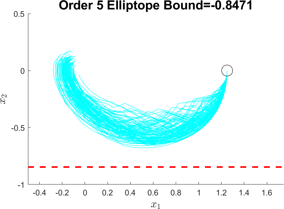
The set in (53b) is the standard convex elliptope/pillow spectahedron. Dynamics in (53) start at X0=[1.25;0]subscript𝑋01.250X_{0}=[1.25;0] and continue for T=5𝑇5T=5 time units in the space X=[0.5,1.75]×[1,0.5]𝑋0.51.7510.5X=[-0.5,1.75]\times[-1,0.5]. The first 6 bounds of maximizing p(x)=x2𝑝𝑥subscript𝑥2p(x)=-x_{2} along these trajectories, after performing a robust counterpart, are p1:6=[1,1,0.8952,0.8477,0.8471,0.8470]subscriptsuperscript𝑝:16110.89520.84770.84710.8470p^{*}_{1:6}=[1,1,0.8952,0.8477,0.8471,0.8470]. At order 666, the largest PSD matrix constraint (for the 3×3333\times 3 SOS-matrix) is of size 3(3+66)=2523binomial3662523\binom{3+6}{6}=252 in the variables (t,x)𝑡𝑥(t,x) after performing robust decomposition, while the non-decomposed largest PSD size is 3(6+66)=27723binomial66627723\binom{6+6}{6}=2772 in the variables (t,x,w)𝑡𝑥𝑤(t,x,w). Sample trajectories of (53) are plotted in Figure 1.
Refer to caption
Figure 1: Order-5 bound on minimal x2subscript𝑥2x_{2} for Flow (53) under elliptope-constrained noise

7.2 Data-Driven Flow System

The uncontrolled Flow system from [45] is

x˙(t)˙𝑥𝑡\displaystyle\dot{x}(t) =[x2(t);x1(t)x2(t)+x13(t)/3]t[0,5].formulae-sequenceabsentsubscript𝑥2𝑡subscript𝑥1𝑡subscript𝑥2𝑡subscriptsuperscript𝑥31𝑡3for-allsuperscript𝑡05\displaystyle=[x_{2}(t);\ -x_{1}(t)-x_{2}(t)+x^{3}_{1}(t)/3]\qquad\forall t^{\prime}\in[0,5]. (54)

This subsection will perform data-driven peak and distance estimation. The derivative x2˙˙subscript𝑥2\dot{x_{2}} is modeled by a cubic polynomial x2˙=degα3wαx1α1x2α2˙subscript𝑥2subscriptdegree𝛼3subscript𝑤𝛼superscriptsubscript𝑥1subscript𝛼1superscriptsubscript𝑥2subscript𝛼2\dot{x_{2}}=\sum_{\deg\alpha\leq 3}w_{\alpha}x_{1}^{\alpha_{1}}x_{2}^{\alpha_{2}} with 10 unknown parameters/inputs {wα}subscript𝑤𝛼\{w_{\alpha}\}. The derivative x˙1=x2subscript˙𝑥1subscript𝑥2\dot{x}_{1}=x_{2} remains known and there is no uncertainty in the first coordinate. The system model for the data-driven flow system is

x˙(t)˙𝑥𝑡\displaystyle\dot{x}(t) =[x2(t);degα3wα(t)x1α1(t)x2α2(t)]t[0,5].formulae-sequenceabsentsubscript𝑥2𝑡subscriptdegree𝛼3subscript𝑤𝛼𝑡superscriptsubscript𝑥1subscript𝛼1𝑡superscriptsubscript𝑥2subscript𝛼2𝑡for-allsuperscript𝑡05\displaystyle=[x_{2}(t);\ \textstyle\sum_{\deg\alpha\leq 3}w_{\alpha}(t)x_{1}^{\alpha_{1}}(t)x_{2}^{\alpha_{2}}(t)]\qquad\forall t^{\prime}\in[0,5]. (55)

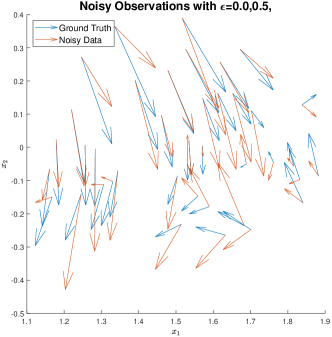
Figure 2 visualizes N=40𝑁40N=40 observed data points sampled within the initial set Xsample={x(x11.5)2+x220.42}subscript𝑋𝑠𝑎𝑚𝑝𝑙𝑒conditional-set𝑥superscriptsubscript𝑥11.52superscriptsubscript𝑥22superscript0.42X_{sample}=\{x\mid(x_{1}-1.5)^{2}+x_{2}^{2}\leq 0.4^{2}\}. The true derivative values are the blue arrows and the ϵ=[0;0.5]italic-ϵ00.5\epsilon=[0;0.5]-corrupted derivative observations are orange. The N=40𝑁40N=40 points yield 2N=802𝑁802N=80 affine constraints, of which the polytope W𝑊W has L=33𝐿33L=33 faces (nonredundant constraints) and 7534 vertices.

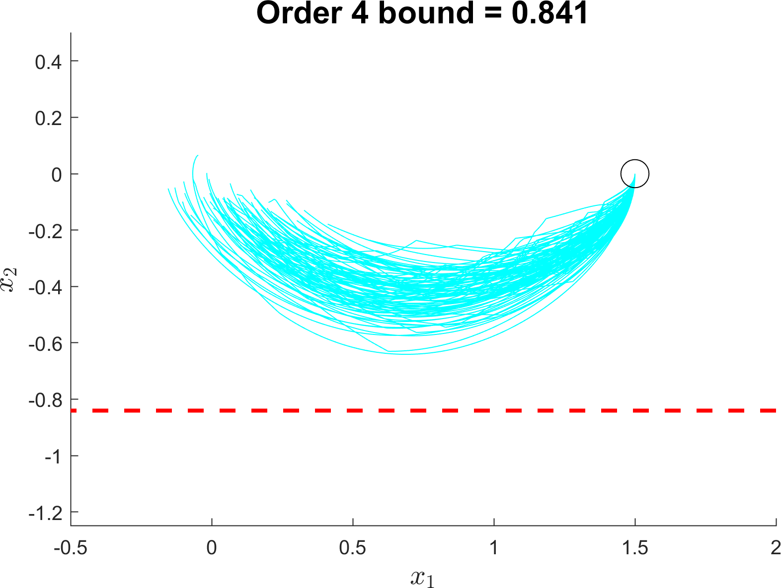
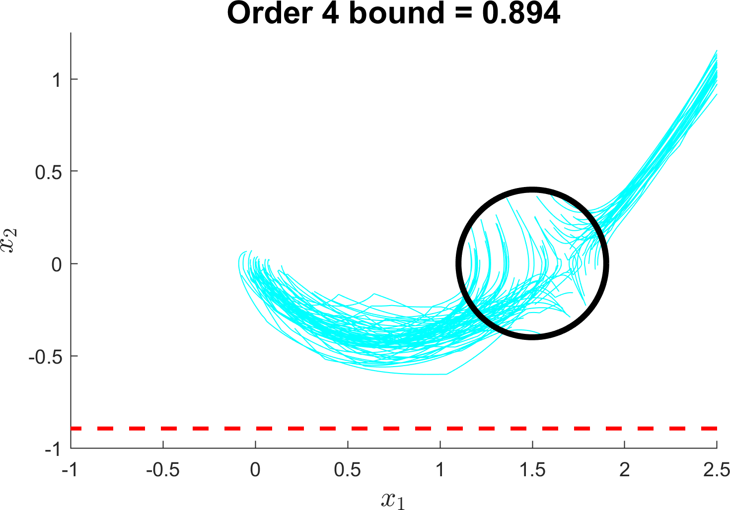
Figure 3 displays system trajectories of (55) for a time horizon of T=5𝑇5T=5 starting from the point X0=(1.5,0)subscript𝑋01.50X_{0}=(1.5,0) (left, Figure 3(a)) and from the circle X0=Xsamplesubscript𝑋0subscript𝑋sampleX_{0}=X_{\text{sample}} (right, Figure 3(b)), when the uncertainty process w(t)𝑤𝑡w(t) is restricted to W𝑊W. Each case desires to maximize p(x)=x2𝑝𝑥subscript𝑥2p(x)=-x_{2} over the state region of X={xx228}𝑋conditional-set𝑥superscriptsubscriptdelimited-∥∥𝑥228X=\{x\mid\lVert x\rVert_{2}^{2}\leq 8\}. The first 4 SOS peak estimates in the point X0subscript𝑋0X_{0} case (Figure 3(a)) are d1:4=[2.828,2.448,1.018,0.8407]superscriptsubscript𝑑:142.8282.4481.0180.8407d_{1:4}^{*}=[2.828,2.448,1.018,0.8407]. The first four estimates in the disc X0subscript𝑋0X_{0} case (Figure 3(b)) are d1:4=[2.828,2.557,1.245,0.894]superscriptsubscript𝑑:142.8282.5571.2450.894d_{1:4}^{*}=[2.828,2.557,1.245,0.894].

Refer to caption
Figure 2: Observed data of Flow system (54) within a circle
Refer to caption
(a) X0=(1.5,0)subscript𝑋01.50X_{0}=(1.5,0)
Refer to caption
(b) X0=Xsamplesubscript𝑋0subscript𝑋sampleX_{0}=X_{\text{sample}}
Figure 3: Minimizing x2subscript𝑥2x_{2} on the observed Flow system (55) at order-4 SOS tightening

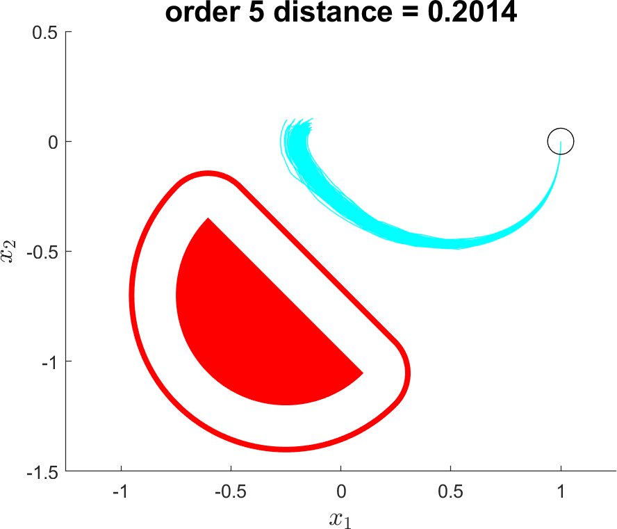
Figure 4 displays the result of distance estimation on the Flow system (55) with N=40𝑁40N=40 points and ϵ=[0;0.5]italic-ϵ00.5\epsilon=[0;0.5]. The initial point is X0=[1;0]subscript𝑋010X_{0}=[1;0] in the state set X=[1,1.25]×[1.25,0.7]𝑋11.251.250.7X=[-1,1.25]\times[-1.25,0.7], and trajectories are tracked for T=5𝑇5T=5 time units. The distance function is the L2subscript𝐿2L_{2} distance and the red half-circle unsafe set is Xu={x0.52(x1+0.25)2(x2+0.7)2,(x1+0.25)/2+(x2+0.7)2/2>=0}subscript𝑋𝑢conditional-set𝑥formulae-sequencesuperscript0.52superscriptsubscript𝑥10.252superscriptsubscript𝑥20.72subscript𝑥10.252superscriptsubscript𝑥20.7220X_{u}=\{x\mid 0.5^{2}\geq-(x_{1}+0.25)^{2}-(x_{2}+0.7)^{2},\-(x_{1}+0.25)/\sqrt{2}+(x_{2}+0.7)^{2}/\sqrt{2}>=0\}. The first 5 bounds of the robust distance estimation program are c1:5=[1.698×10⁵, 0.1936, 0.2003, 0.2009, 0.2013]subscriptsuperscript𝑐:151.698superscript1050.19360.20030.20090.2013c^{*}_{1:5}=[1.698\times 10^{-5},\ 0.1936,\ 0.2003,\ 0.2009,\ 0.2013].

Refer to caption
Figure 4: Distance estimate of (54) at order 5

7.3 Twist System

This section performs peak estimation on the Twist system from [9]

x˙i(t)subscript˙𝑥𝑖𝑡\displaystyle\dot{x}_{i}(t) =jBij1xj(t)Bij3(4xj3(t)3xj(t))/2,absentsubscript𝑗subscriptsuperscript𝐵1𝑖𝑗subscript𝑥𝑗𝑡subscriptsuperscript𝐵3𝑖𝑗4superscriptsubscript𝑥𝑗3𝑡3subscript𝑥𝑗𝑡2\displaystyle=\textstyle\sum_{j}B^{1}_{ij}x_{j}(t)-B^{3}_{ij}(4x_{j}^{3}(t)-3x_{j}(t))/2, (56)
B1superscript𝐵1\displaystyle B^{1} =[111101012]absentmatrix111101012\displaystyle=\begin{bmatrix}-1&1&1\\ -1&0&-1\\ 0&1&-2\end{bmatrix} B3superscript𝐵3\displaystyle B^{3} =[101011110].absentmatrix101011110\displaystyle=\begin{bmatrix}-1&0&-1\\ 0&1&1\\ 1&1&0\end{bmatrix}. (57)

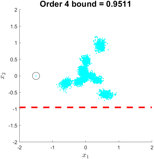
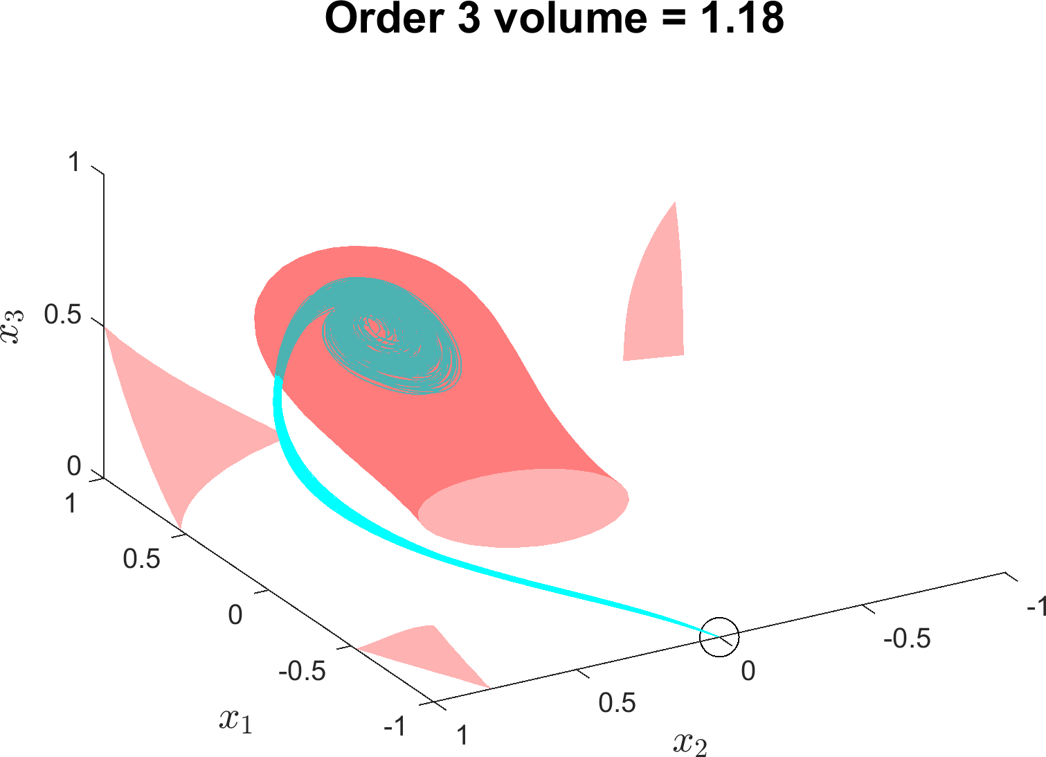
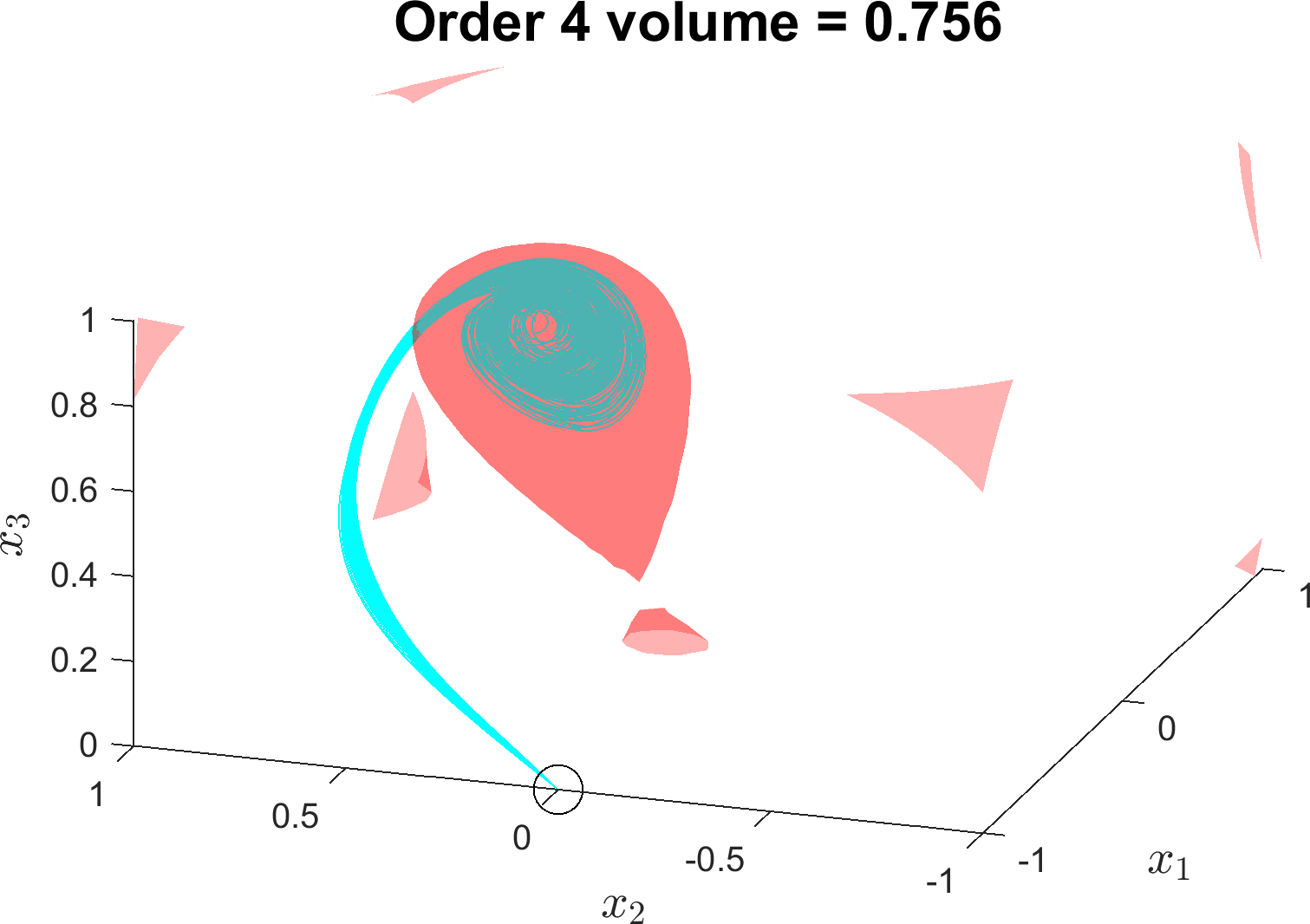
Choosing different parameter matrices B1superscript𝐵1B^{1} (linear) and B3superscript𝐵3B^{3} (cubic) yields a family of dynamical systems, many of which are attractors and some of which possess limit cycles. We note that the Twist system possesses a symmetry xx𝑥𝑥x\leftrightarrow-x, and therefore only the top portion with x30subscript𝑥30x_{3}\geq 0 will be treated. A total of N=100𝑁100N=100 observations with a noise bound of ϵ=0.5italic-ϵ0.5\epsilon=0.5 are taken, and are plotted in Figure 5. These N=100𝑁100N=100 observations will induce 2Nn=6002𝑁𝑛6002Nn=600 affine constraints on eventual polytopes W𝑊W.

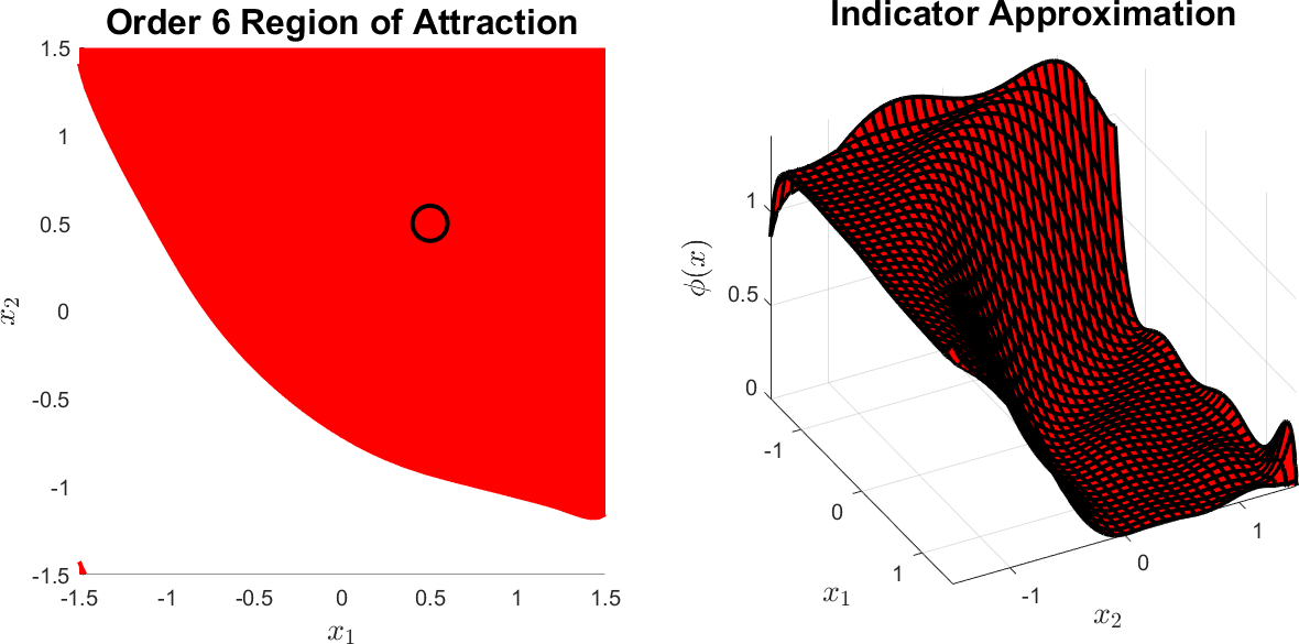
Details of the auxiliary function LPs for distance estimation, reachable set estimation, and ROA maximization are found in Appendix E. The decomposable Lie constraints in these problems (from Appendix E) are (107c), (108d), and (109d) respectively.
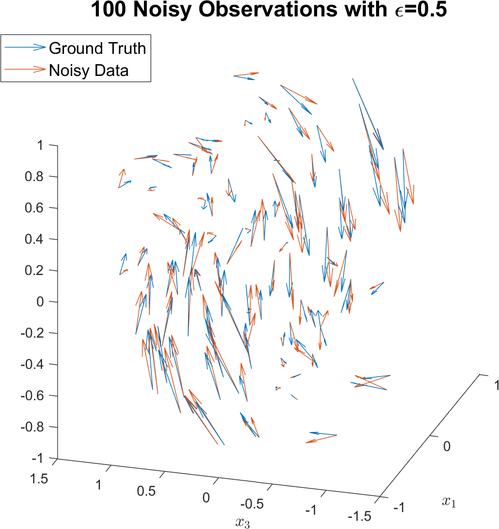
Refer to caption
Figure 5: 100 observations of Twist system (56)

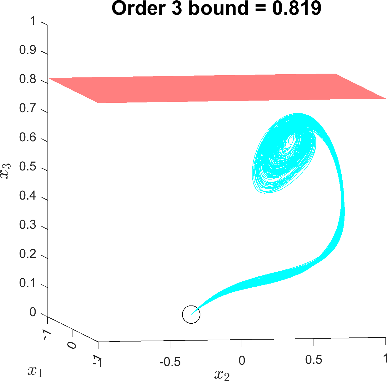
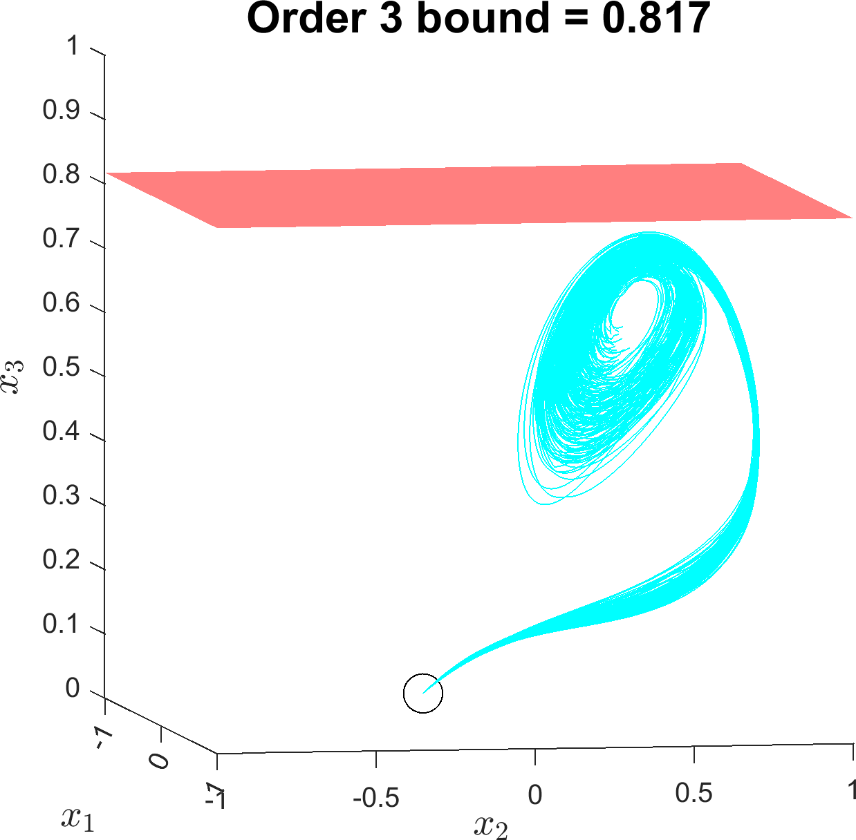
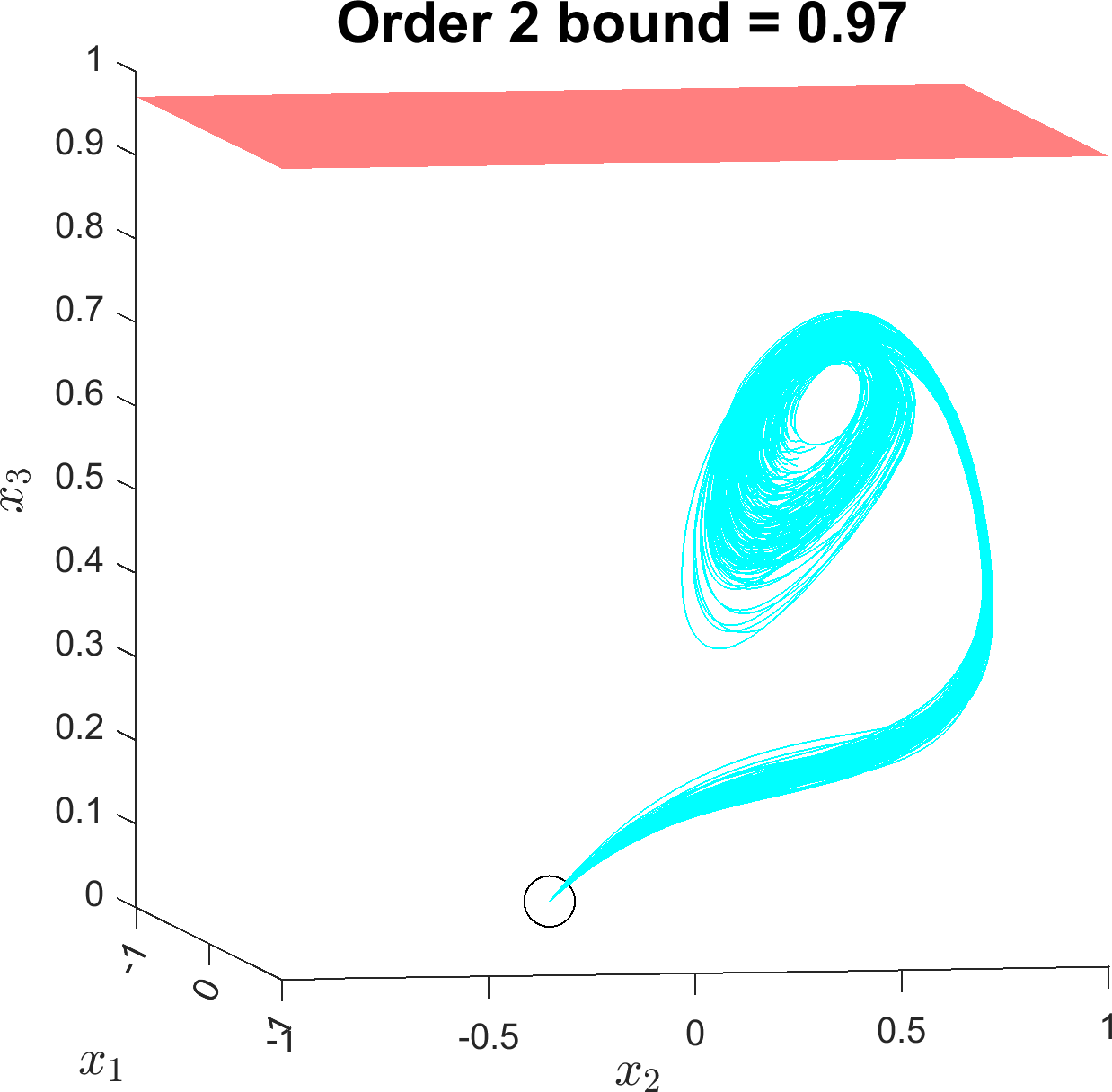
All scenarios in this subsection will find peak estimates on the maximum value of p(x)=x3𝑝𝑥subscript𝑥3p(x)=x_{3} of the Twist system over the space X={x1x1,x21, 0x31}𝑋conditional-set𝑥formulae-sequence1subscript𝑥1formulae-sequencesubscript𝑥21 0subscript𝑥31X=\{x\mid-1\leq x_{1},x_{2}\leq 1,\ 0\leq x_{3}\leq 1\} and time horizon T=8𝑇8T=8 starting at X0=[1,0,0]subscript𝑋0100X_{0}=[-1,0,0].

Figure 6 involves the L=9𝐿9L=9 case where B1superscript𝐵1B^{1} is unknown (left) or when B3superscript𝐵3B^{3} is unknown (right). When B1superscript𝐵1B^{1} is unknown, the matrix B1superscript𝐵1B^{1} in (57) is replaced by a matrix of parameter inputs w:[0,T]3×3:𝑤0𝑇superscript33w:[0,T]\rightarrow\mathbb{R}^{3\times 3} according to Remark 12 (with a similar substitution in the unknown B3superscript𝐵3B^{3} case).

The unknown B1superscript𝐵1B^{1} case in Figure 6(a) has a polytope W𝑊W with m=30𝑚30m=30 faces and peak bounds of d1:3=[1.000,0.9050,0.8174]superscriptsubscript𝑑:131.0000.90500.8174d_{1:3}^{*}=[1.000,0.9050,0.8174]. The known B3superscript𝐵3B^{3} case in Figure 6(b) also has m=30𝑚30m=30 faces in its polytope with peak bounds of d1:3=[1.000,0.9050,0.8174]superscriptsubscript𝑑:131.0000.90500.8174d_{1:3}^{*}=[1.000,0.9050,0.8174]. The maximal PSD matrix size of the Lie nonpositivity constraint is 2380 pre-decomposition and 70 post-decomposition. Computational limits of the experimental platform restricted the computation of dsuperscript𝑑d^{*} to maximal order 3 .

Refer to caption
(a) Unknown B1superscript𝐵1B^{1}, Known B3superscript𝐵3B^{3}
Refer to caption
(b) Known B1superscript𝐵1B^{1}, Unknown B3superscript𝐵3B^{3}
Figure 6: Twist (56) system where either B1superscript𝐵1B^{1} or B3superscript𝐵3B^{3} are unknown.

When both parameters (B1,B3)superscript𝐵1superscript𝐵3(B^{1},B^{3}) are unknown, the polytope W𝑊W has L=18𝐿18L=18 dimensions and m=70𝑚70m=70 nonredundant faces. The first peak estimates on this system are d1:2=[1.000,0.9703]superscriptsubscript𝑑:121.0000.9703d_{1:2}^{*}=[1.000,0.9703] as plotted in Figure 7. At degree 2, the maximal PSD matrix size in the Lie constraint falls from 2300 pre-decomposition and to 35 post-decomposition. The experimental platform became unresponsive in YALMIP when attempting to compile the d3subscriptsuperscript𝑑3d^{*}_{3} model when (B1,B3)superscript𝐵1superscript𝐵3(B^{1},B^{3}) are unknown.

Refer to caption
Figure 7: Twist (56) with unknown (B1,B3)superscript𝐵1superscript𝐵3(B^{1},B^{3})

7.4 Discrete-Time Peak Estimation Example

This example performs peak estimation (41) on a discrete-time system. The ground-truth system is ((35a) from [16])

x+=[0.3x1+0.8x2+0.1x1x20.75x10.3x2+w]subscript𝑥matrix0.3subscript𝑥10.8subscript𝑥20.1subscript𝑥1subscript𝑥20.75subscript𝑥10.3subscript𝑥2𝑤x_{+}=\begin{bmatrix}-0.3x_{1}+0.8x_{2}+0.1x_{1}x_{2}\\ -0.75x_{1}-0.3x_{2}+w\end{bmatrix} (58)

The system model for (58) is a quadratic polynomial vector with unknown coefficients (w1,w2)superscript𝑤1superscript𝑤2(w^{1},w^{2}):

x+=[degα2wα1x1α1x2α2,degα2wα2x1α1x2α2]Tsubscript𝑥superscriptmatrixsubscriptdegree𝛼2subscriptsuperscript𝑤1𝛼subscriptsuperscript𝑥subscript𝛼11subscriptsuperscript𝑥subscript𝛼22subscriptdegree𝛼2subscriptsuperscript𝑤2𝛼subscriptsuperscript𝑥subscript𝛼11subscriptsuperscript𝑥subscript𝛼22𝑇x_{+}=\begin{bmatrix}\sum_{\deg\alpha\leq 2}w^{1}_{\alpha}x^{\alpha_{1}}_{1}x^{\alpha_{2}}_{2},&\ \sum_{\deg\alpha\leq 2}w^{2}_{\alpha}x^{\alpha_{1}}_{1}x^{\alpha_{2}}_{2}\end{bmatrix}^{T} (59)

The model in (59) has L=12𝐿12L=12 unknown parameters (w1,w2)superscript𝑤1superscript𝑤2(w^{1},w^{2}). Sampling over X=[2,2]2𝑋superscript222X=[-2,2]^{2} occurs Ns=40subscript𝑁𝑠40N_{s}=40 times, yielding observations corrupted by Lsubscript𝐿L_{\infty}-bounded noise (ϵ=0.5italic-ϵ0.5\epsilon=0.5).

The observed data for state transitions are pictured in Figure 8(a). It is desired to bound the maximum value of p(x)=x2𝑝𝑥subscript𝑥2p(x)=-x_{2} along discrete-time system trajectories up to a time horizon of T=10𝑇10T=10. With a starting point of X0=[1.5,0]subscript𝑋01.50X_{0}=[-1.5,0], SOS tightenings of the discrete-time peak estimation program in (48) produce bounds of d1:4=[2.0000,1.7221,1.1254,0.9511]subscriptsuperscript𝑑:142.00001.72211.12540.9511d^{*}_{1:4}=[2.0000,1.7221,1.1254,0.9511]. The order-4 bound is pictured in Figure 8(b).
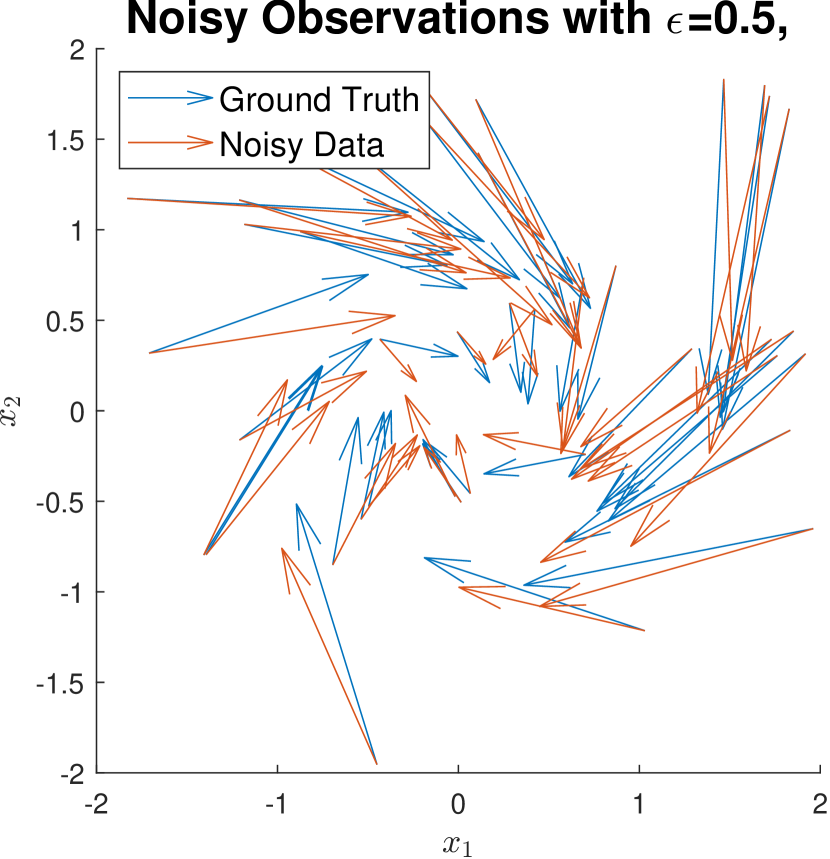
Refer to caption
(a) Observed data of (58)
Refer to caption
(b) Order 4 tightening
Figure 8: Peak p(x)=x2𝑝𝑥subscript𝑥2p(x)=-x_{2} estimation of (8(a)) for system model (59) with Lsubscript𝐿L_{\infty}: ϵ=0.5italic-ϵ0.5\epsilon=0.5 corrupted data

7.5 Reachable Set Example

Figure 9 illustrates data-driven reachable set estimation on the Twist system from (56) for a time horizon of T=8𝑇8T=8 by SOS tightening to the Lie-robustified (108). The 100 observations from this system are pictured in Figure 5, yielding a L=9𝐿9L=9-dimensional polytope with 34 non-redundant faces. As the order of tightening to program increases from 3 to 4, the red region (level set of ω(x)𝜔𝑥\omega(x)) tightens to the spiraling attractor region of the T=8𝑇8T=8 reachable set. The reachable set computation problem from (108) involves auxiliary functions v(t,x)𝑣𝑡𝑥v(t,x) and ϕ(x)italic-ϕ𝑥\phi(x), such that ϕ(x)0italic-ϕ𝑥0\phi(x)\geq 0 over X𝑋X and ϕ(x)1italic-ϕ𝑥1\phi(x)\geq 1 over the true T𝑇T-reachable set (14). The ‘volume’ in the plot titles is not the true volume of the superlevel set {xϕ(x)1}conditional-set𝑥italic-ϕ𝑥1\{x\mid\phi(x)\geq 1\}, but is instead the integration of the polynomial ϕ(x)italic-ϕ𝑥\phi(x) over the Lebesgue measure as Xϕ(x)𝑑xsubscript𝑋italic-ϕ𝑥differential-d𝑥\int_{X}\phi(x)dx.

Refer to caption
(a) Order 3 tightening
Refer to caption
(b) Order 4 tightening
Figure 9: Reachable set estimation of twist (56) system where B1superscript𝐵1B^{1} is known and B3superscript𝐵3B^{3} are unknown.

7.6 Region of Attraction Example

This example of ROA maximization will concentrate on a controlled version of the Flow dynamics from [45] under L=6𝐿6L=6 inputs

x˙=[x2(t)x1(t)x2(t)+x13(t)/3]+[w1+w2x1+w3x2w4+w5x1+w6x2]˙𝑥matrixsubscript𝑥2𝑡subscript𝑥1𝑡subscript𝑥2𝑡subscriptsuperscript𝑥31𝑡3matrixsubscript𝑤1subscript𝑤2subscript𝑥1subscript𝑤3subscript𝑥2subscript𝑤4subscript𝑤5subscript𝑥1subscript𝑤6subscript𝑥2\dot{x}=\begin{bmatrix}x_{2}(t)\\ -x_{1}(t)-x_{2}(t)+x^{3}_{1}(t)/3\end{bmatrix}+\begin{bmatrix}w_{1}+w_{2}x_{1}+w_{3}x_{2}\\ w_{4}+w_{5}x_{1}+w_{6}x_{2}\end{bmatrix} (60)

obeying the polytopic input limits

W={w[w1;w4]0.1,[w2;w3;w5;w6]0.15[(w1+w2+w3);(w4+w5+w6)]0.3}.𝑊conditional-set𝑤matrixformulae-sequencesubscriptdelimited-∥∥subscript𝑤1subscript𝑤40.1subscriptdelimited-∥∥subscript𝑤2subscript𝑤3subscript𝑤5subscript𝑤60.15subscriptdelimited-∥∥subscript𝑤1subscript𝑤2subscript𝑤3subscript𝑤4subscript𝑤5subscript𝑤60.3W=\left\{w\mid\begin{matrix}\lVert[w_{1};w_{4}]\rVert_{\infty}\leq 0.1,\ \lVert[w_{2};w_{3};w_{5};w_{6}]\rVert_{\infty}\leq 0.15\\ \lVert[(w_{1}+w_{2}+w_{3});(w_{4}+w_{5}+w_{6})]\rVert_{\infty}\leq 0.3\end{matrix}\right\}. (61)

The circle XT={x0.12(x10.5)2(x20.5)20}subscript𝑋𝑇conditional-set𝑥superscript0.12superscriptsubscript𝑥10.52superscriptsubscript𝑥20.520X_{T}=\{x\mid 0.1^{2}-(x_{1}-0.5)^{2}-(x_{2}-0.5)^{2}\geq 0\} is the destination of the ROA problem with a time horizon of T=5𝑇5T=5 and a state space of X=[1.5,1.5]2𝑋superscript1.51.52X=[-1.5,1.5]^{2}. The WSOS tightening of problem the Lie-robustified (109) yields bounds for the ROA volume of d2:6=[9.000, 9.000, 6.717, 5.620, 5.187].subscriptsuperscript𝑑:269.0009.0006.7175.6205.187d^{*}_{2:6}=[9.000,\ 9.000,\ 6.717,\ 5.620,\ 5.187].

The destination set XTsubscript𝑋𝑇X_{T} is drawn in the black circle in the left subplot of Figure 10. The white area is an outer approximation of the true ROA, found as the superlevel set {xϕ(x)1}conditional-set𝑥italic-ϕ𝑥1\{x\mid\phi(x)\geq 1\} at order 6. The red area is the sublevel set {xϕ(x)1}conditional-set𝑥italic-ϕ𝑥1\{x\mid\phi(x)\leq 1\}. The right subplot of Figure 10 draws the degree-12 polynomial function ϕ(x)italic-ϕ𝑥\phi(x).

Refer to caption
Figure 10: Order 6 ROA for controlled Flow (60)

8 Conclusion

This work formulated infinite-dimensional robust counterparts decomposing input-affine Lie constraints in analysis and control problems. These robust counterparts may be approximated by continuous multipliers without conservatism under compactness and regularity conditions. Elimination of the noise variables w𝑤w allows for solution and analysis of formerly intractable problems using the moment-SOS hierarchy. The robust counterpart method was demonstrated on peak estimation, distance estimation, reachable set estimation, and BRS-maximizing control problems. Another environment in which these robust counterparts may be employed is in data-driven systems analysis with affinely-parameterized dictionaries and SDR noise.

The robust counterpart method may be used in other optimization domains with Lie constraints, such as in optimal control input penalties [5] and maximum controlled invariant set estimation [46].

One future research direction is to investigate other types of exploitable uncertainty structure in dynamical systems problems. Another avenue is to incorporate warm starts into SDP solvers so online system estimates can be updated as more data gets added to 𝒟𝒟\mathcal{D}. The bottleneck of all computations developed in this paper is the compuational cost of the SOS tightenings, so finding ways to speed up SOS-based SDP solution is of vital interest. An important research path from a theoretical perspective is finding circumstances in which Assumption A6’ can be relaxed while still obeying polynomial approximability Theorem 3.2.

Acknowledgements

The authors would like to thank Didier Henrion, Milan Korda, Victor Magron, and Roy Smith for their advice and support. The authors would also like to thank Carsten Scherer for discussions about the proof of Proposition B.4.

References

  • [1] J. W. Helton and J. Nie, “Semidefinite representation of convex sets,” Mathematical Programming, vol. 122, pp. 21–64, 2010.
  • [2] A. Ben-Tal, L. El Ghaoui, and A. Nemirovski, Robust Optimization.   Princeton University Press, 2009, vol. 28.
  • [3] S. Boyd, S. P. Boyd, and L. Vandenberghe, Convex Optimization.   Cambridge university press, 2004.
  • [4] A. Ben-Tal, D. Den Hertog, and J.-P. Vial, “Deriving robust counterparts of nonlinear uncertain inequalities,” Mathematical programming, vol. 149, no. 1-2, pp. 265–299, 2015.
  • [5] A. Majumdar, R. Vasudevan, M. M. Tobenkin, and R. Tedrake, “Convex Optimization of Nonlinear Feedback Controllers via Occupation Measures,” The International Journal of Robotics Research, vol. 33, no. 9, pp. 1209–1230, 2014.
  • [6] M. Korda, D. Henrion, and C. N. Jones, “Controller design and value function approximation for nonlinear dynamical systems,” Automatica, vol. 67, pp. 54–66, 2016.
  • [7] J. Miller and M. Sznaier, “Facial Input Decompositions for Robust Peak Estimation under Polyhedral Uncertainty,” IFAC-PapersOnLine, vol. 55, no. 25, pp. 55–60, 2022, 10th IFAC Symposium on Robust Control Design 2022.
  • [8] M. J. Cho and R. H. Stockbridge, “Linear Programming Formulation for Optimal Stopping Problems,” SIAM Journal on Control and Optimization, vol. 40, no. 6, pp. 1965–1982, 2002.
  • [9] J. Miller and M. Sznaier, “Bounding the Distance to Unsafe Sets with Convex Optimization,” IEEE Trans. Automat. Contr., pp. 1–15, 2023.
  • [10] J.-P. Aubin, A. M. Bayen, and P. Saint-Pierre, Viability theory: new directions.   Springer Science & Business Media, 2011.
  • [11] I. M. Mitchell and C. J. Tomlin, “Overapproximating reachable sets by hamilton-jacobi projections,” journal of Scientific Computing, vol. 19, no. 1, pp. 323–346, 2003.
  • [12] R. Lewis and R. Vinter, “Relaxation of Optimal Control Problems to Equivalent Convex Programs,” Journal of Mathematical Analysis and Applications, vol. 74, no. 2, pp. 475–493, 1980.
  • [13] D. Henrion, J. B. Lasserre, and C. Savorgnan, “Nonlinear optimal control synthesis via occupation measures,” in 2008 47th IEEE Conference on Decision and Control.   IEEE, 2008, pp. 4749–4754.
  • [14] G. Fantuzzi and D. Goluskin, “Bounding Extreme Events in Nonlinear Dynamics Using Convex Optimization,” SIAM Journal on Applied Dynamical Systems, vol. 19, no. 3, pp. 1823–1864, 2020.
  • [15] J. Miller, D. Henrion, and M. Sznaier, “Peak Estimation Recovery and Safety Analysis,” IEEE Control Systems Letters, pp. 1–1, 2020.
  • [16] J. Miller, D. Henrion, M. Sznaier, and M. Korda, “Peak Estimation for Uncertain and Switched Systems,” in 2021 60th IEEE Conference on Decision and Control (CDC), 2021, pp. 3222–3228.
  • [17] D. Henrion and M. Korda, “Convex computation of the region of attraction of polynomial control systems,” IEEE Trans. Automat. Contr., vol. 59, no. 2, p. 297–312, Feb 2014.
  • [18] M. Korda, D. Henrion, and C. N. Jones, “Inner approximations of the region of attraction for polynomial dynamical systems,” IFAC Proceedings Volumes, vol. 46, no. 23, pp. 534–539, 2013.
  • [19] A. Majumdar, A. A. Ahmadi, and R. Tedrake, “Control design along trajectories with sums of squares programming,” in 2013 IEEE International Conference on Robotics and Automation.   IEEE, 2013, pp. 4054–4061.
  • [20] A. B. Kurzhanski and P. Varaiya, “On ellipsoidal techniques for reachability analysis. part i: external approximations,” Optimization methods and software, vol. 17, no. 2, pp. 177–206, 2002.
  • [21] S. M. Harwood and P. I. Barton, “Efficient polyhedral enclosures for the reachable set of nonlinear control systems,” Mathematics of Control, Signals, and Systems, vol. 28, no. 1, p. 8, 2016.
  • [22] S. Coogan, “Mixed monotonicity for reachability and safety in dynamical systems,” in 2020 59th IEEE Conference on Decision and Control (CDC).   IEEE, 2020, pp. 5074–5085.
  • [23] J. J. Bramburger and G. Fantuzzi, “Auxiliary functions as koopman observables: Data-driven polynomial optimization for dynamical systems,” arXiv preprint arXiv:2303.01483, 2023.
  • [24] T. Dai and M. Sznaier, “A Semi-Algebraic Optimization Approach to Data-Driven Control of Continuous-Time Nonlinear Systems,” IEEE Control Systems Letters, vol. 5, no. 2, pp. 487–492, 2020.
  • [25] C. W. Scherer and C. W. Hol, “Matrix Sum-of-Squares Relaxations for Robust Semi-Definite Programs,” Mathematical programming, vol. 107, no. 1, pp. 189–211, 2006.
  • [26] M. Putinar, “Positive Polynomials on Compact Semi-algebraic Sets,” Indiana University Mathematics Journal, vol. 42, no. 3, pp. 969–984, 1993.
  • [27] J. B. Lasserre, Moments, Positive Polynomials And Their Applications, ser. Imperial College Press Optimization Series.   World Scientific Publishing Company, 2009.
  • [28] C. Hol and C. Scherer, “Sum of squares relaxations for robust polynomial semi-definite programs,” IFAC Proceedings Volumes, vol. 38, no. 1, pp. 451–456, 2005.
  • [29] D. Henrion and M. Korda, “Convex computation of the region of attraction of polynomial control systems,” IEEE Trans. Automat. Contr., vol. 59, no. 2, p. 297–312, Feb 2014.
  • [30] A. Abate, D. Ahmed, A. Edwards, M. Giacobbe, and A. Peruffo, “Fossil: a software tool for the formal synthesis of lyapunov functions and barrier certificates using neural networks,” in Proceedings of the 24th International Conference on Hybrid Systems: Computation and Control, 2021, pp. 1–11.
  • [31] D. Papp and F. Alizadeh, “Semidefinite characterization of sum-of-squares cones in algebras,” SIAM journal on optimization, vol. 23, no. 3, pp. 1398–1423, 2013.
  • [32] F. Alizadeh and D. Goldfarb, “Second-order cone programming,” Mathematical programming, vol. 95, no. 1, pp. 3–51, 2003.
  • [33] Y. Zheng and G. Fantuzzi, “Sum-of-squares chordal decomposition of polynomial matrix inequalities,” Mathematical Programming, vol. 197, no. 1, pp. 71–108, 2023.
  • [34] W. Han and R. Tedrake, “Controller synthesis for discrete-time polynomial systems via occupation measures,” 2018 IEEE/RSJ International Conference on Intelligent Robots and Systems (IROS), Oct 2018.
  • [35] J. Miller and M. Sznaier, “Peak Estimation of Hybrid Systems with Convex Optimization,” 2023, arxiv:2303.11490.
  • [36] Y. Cheng, M. Sznaier, and C. Lagoa, “Robust Superstabilizing Controller Design from Open-Loop Experimental Input/Output Data,” IFAC-PapersOnLine, vol. 48, no. 28, pp. 1337–1342, 2015.
  • [37] T. Dai and M. Sznaier, “A Moments Based Approach to Designing MIMO Data Driven Controllers for Switched Systems,” in 2018 IEEE Conference on Decision and Control (CDC).   IEEE, 2018, pp. 5652–5657.
  • [38] T. Martin, T. B. Schön, and F. Allgöwer, “Gaussian inference for data-driven state-feedback design of nonlinear systems,” arXiv preprint arXiv:2211.05639, 2022.
  • [39] H. J. van Waarde, M. K. Camlibel, and M. Mesbahi, “From noisy data to feedback controllers: non-conservative design via a Matrix S-Lemma,” IEEE Trans. Automat. Contr., 2020.
  • [40] R. Caron, J. McDonald, and C. Ponic, “A degenerate extreme point strategy for the classification of linear constraints as redundant or necessary,” Journal of Optimization Theory and Applications, vol. 62, no. 2, pp. 225–237, 1989.
  • [41] J. Löfberg, “YALMIP : A Toolbox for Modeling and Optimization in MATLAB,” in In Proceedings of the CACSD Conference, Taipei, Taiwan, 2004.
  • [42] M. ApS, The MOSEK optimization toolbox for MATLAB manual. Version 9.2., 2020. [Online]. Available: https://docs.mosek.com/9.2/toolbox/index.html
  • [43] D. P. Kroese, T. Taimre, and Z. I. Botev, Handbook of monte carlo methods.   John Wiley & Sons, 2013, vol. 706.
  • [44] T. Benham, “Uniform distribution over a convex polytope,” 2012. [Online]. Available: https://www.mathworks.com/matlabcentral/fileexchange/34208-uniform-distribution-over-a-convex-polytope
  • [45] S. Prajna and A. Jadbabaie, “Safety Verification of Hybrid Systems Using Barrier Certificates,” in International Workshop on Hybrid Systems: Computation and Control.   Springer, 2004, pp. 477–492.
  • [46] M. Korda, D. Henrion, and C. Jones, “Convex Computation of the Maximum Controlled Invariant Set For Polynomial Control Systems,” SIAM Journal on Control and Optimization, vol. 52, no. 5, pp. 2944–2969, 2014.
  • [47] J. G. Llavona, Approximation of continuously differentiable functions.   Elsevier, 1986.
  • [48] J.-P. Aubin and H. Frankowska, Set-Valued Analysis.   Springer Science & Business Media, 2009.
  • [49] R. T. Rockafellar and R. J.-B. Wets, Variational Analysis.   Springer Science & Business Media, 2009, vol. 317.
  • [50] J. Denel, “Extensions of the continuity of point-to-set maps: applications to fixed point algorithms,” Point-to-Set Maps and Mathematical Programming, pp. 48–68, 1979.
  • [51] E. Stiemke, “Über positive lösungen homogener linearer gleichungen,” Mathematische Annalen, vol. 76, no. 2-3, pp. 340–342, 1915.
  • [52] A. Daniilidis, M. A. Goberna, M. A. López, and R. Lucchetti, “Lower semicontinuity of the feasible set mapping of linear systems relative to their domains,” Set-Valued and Variational Analysis, vol. 21, no. 1, pp. 67–92, 2013.
  • [53] R. Henrion and A. Seeger, “On Properties of Different Notions of Centers for Convex Cones,” Set-Valued and Variational Analysis, vol. 18, pp. 205–231, 2010.
  • [54] ——, “Inradius and Circumradius of Various Convex Cones Arising in Applications,” Set-Valued and Variational Analysis, vol. 18, pp. 483–511, 2010.
  • [55] T. Tao, An Introduction to Measure Theory.   American Mathematical Society Providence, RI, 2011, vol. 126.
  • [56] M. Pivato, “Analysis, Measure, and Probability: A visual introduction,” 2003.
  • [57] L. C. Young, “Generalized Surfaces in the Calculus of Variations,” Annals of mathematics, vol. 43, pp. 84–103, 1942.
  • [58] D. Liberzon, Calculus of Variations and Optimal Control Theory: A Concise Introduction.   Princeton University Press, 2011.
  • [59] J. Gouveia, P. A. Parrilo, and R. R. Thomas, “Lifts of Convex Sets and Cone Factorizations,” Mathematics of Operations Research, vol. 38, no. 2, pp. 248–264, 2013.

Appendix A Polynomial Approximation of the Auxiliary Function

This appendix uses arguments from [14] to prove that Problem (18) may be approximated with ε𝜀\varepsilon-accuracy by a polynomial auxiliary function. Assumptions A1-A4 are in place, ensuring that Ω=[0,T]×X×WΩ0𝑇𝑋𝑊\Omega=[0,T]\times X\times W is compact.

Let ε>0𝜀0\varepsilon>0 be an optimality bound, and let v(t,x)C1([0,T]×X)𝑣𝑡𝑥superscript𝐶10𝑇𝑋v(t,x)\in C^{1}([0,T]\times X) be an auxiliary function that satisfies constraints (18c) and (18d) with

supxX0v(0,x)d+ε.subscriptsupremum𝑥subscript𝑋0𝑣0𝑥superscript𝑑𝜀\sup_{x\in X_{0}}v(0,x)\leq d^{*}+\varepsilon. (62)

The i𝑖i-th coordinate of dynamics x˙=F(t,x,w)=f0(t,x)+w=1Lwf(t,x)˙𝑥𝐹𝑡𝑥𝑤subscript𝑓0𝑡𝑥superscriptsubscript𝑤1𝐿subscript𝑤subscript𝑓𝑡𝑥\dot{x}=F(t,x,w)=f_{0}(t,x)+\sum_{w=1}^{L}w_{\ell}f_{\ell}(t,x) from (1) is indexed by Fi(t,x,w)subscript𝐹𝑖𝑡𝑥𝑤F_{i}(t,x,w).

A tolerance η>0𝜂0\eta>0 may be chosen as (Equation 4.10 of [14]):

η<εmax(2,2T,2TF1C0(Ω),,2TFnC0(Ω)).𝜂𝜀22𝑇2𝑇subscriptdelimited-∥∥subscript𝐹1superscript𝐶0Ω2𝑇subscriptdelimited-∥∥subscript𝐹𝑛superscript𝐶0Ω\displaystyle\eta<\frac{\varepsilon}{\max\left(2,2T,2T\lVert F_{1}\rVert_{C^{0}(\Omega)},\ldots,2T\lVert F_{n}\rVert_{C^{0}(\Omega)}\right)}. (63)

A polynomial approximation of the C1superscript𝐶1C^{1} function v𝑣v may be performed by Theorem 1.1.2 of [47] to find a polynomial w[t,x]𝑤𝑡𝑥w\in\mathbb{R}[t,x] such that v(t,x)w(t,x)C1(Ω)<ηsubscriptdelimited-∥∥𝑣𝑡𝑥𝑤𝑡𝑥superscript𝐶1Ω𝜂\lVert v(t,x)-w(t,x)\rVert_{C^{1}(\Omega)}<\eta uniformly. The perturbed auxiliary function,

V(t,x)=w(t,x)+ε(1t/(2T)),𝑉𝑡𝑥𝑤𝑡𝑥𝜀1𝑡2𝑇V(t,x)=w(t,x)+\varepsilon(1-t/(2T)), (64)

satisfies the following strict inequalities from (18) (equation 4.12 in [14]),

d+(5/2)ε>V(0,x)superscript𝑑52𝜀𝑉0𝑥\displaystyle d^{*}+(5/2)\varepsilon>V(0,x) xX0for-all𝑥subscript𝑋0\displaystyle\forall x\in X_{0} (65a)
F(t,x,w)V(t,x)<0subscript𝐹𝑡𝑥𝑤𝑉𝑡𝑥0\displaystyle\mathcal{L}_{F(t,x,w)}V(t,x)<0 (t,x,w)Ωfor-all𝑡𝑥𝑤Ω\displaystyle\forall(t,x,w)\in\Omega (65b)
V(t,x)<p(x)𝑉𝑡𝑥𝑝𝑥\displaystyle V(t,x)<p(x) (t,x)[0,T]×X.for-all𝑡𝑥0𝑇𝑋\displaystyle\forall(t,x)\in[0,T]\times X. (65c)

There then exists some finite d𝑑d such that the polynomial V(t,x)𝑉𝑡𝑥V(t,x) with an optimal solution of (at most) d+(5/2)εsuperscript𝑑52𝜀d^{*}+(5/2)\varepsilon has degree d𝑑d [14].

Appendix B Continuity of Multipliers

This section will prove the continuous selection portion of Theorem 3.2.

B.1 Set-Valued Preliminaries

We first review concepts in set-valued analysis. Given spaces Y𝑌Y and Z𝑍Z, a set-valued function F:YZ:𝐹𝑌𝑍F:Y\rightrightarrows Z is a mapping between the power sets F:2Y2Z:𝐹superscript2𝑌superscript2𝑍F:2^{Y}\rightarrow 2^{Z}. A set EY𝐸𝑌E\subset Y is inside the domain Dom(F)Dom𝐹\text{Dom}(F) if F(E)𝐹𝐸F(E)\neq\varnothing. In this section, we will be utilizing point-set maps (F:Y2Z):𝐹𝑌superscript2𝑍(F:Y\rightarrow 2^{Z}).

Definition B.1 (Definition 1.4.2 of [48]).

The function F𝐹F is lower semicontinuous at yDom(F)𝑦Dom𝐹y\in\text{Dom}(F) if, for every sequence {yk}subscript𝑦𝑘\{y_{k}\} converging to y𝑦y ({yk}ysubscript𝑦𝑘𝑦\{y_{k}\}\rightarrow y), there exists a converging sequence {zkF(y)}subscript𝑧𝑘𝐹𝑦\{z_{k}\in F(y)\} converging to an element zF(y)𝑧𝐹𝑦z\in F(y). The map F𝐹F is lower semicontinuous if it is lower semicontinuous at each yDom(F)𝑦Dom𝐹y\in\text{Dom}(F).

Definition B.2.

Let F0,F1subscript𝐹0subscript𝐹1F_{0},F_{1} be set-valued maps YZ𝑌𝑍Y\rightrightarrows Z. The containment relation F0F1subscript𝐹0subscript𝐹1F_{0}\subseteq F_{1} holds if yY:F0(y)F1(y):for-all𝑦𝑌subscript𝐹0𝑦subscript𝐹1𝑦\forall y\in Y:\ F_{0}(y)\subseteq F_{1}(y).

Remark 13.

Lower semicontinuity in Definition B.1 is also called inner semicontinuity in [49].

Definition B.3 (Definition 1 of [50]).

A family of set-valued maps {Sρ:YZ}ρ0subscriptconditional-setsubscript𝑆𝜌𝑌𝑍𝜌0\{S_{\rho}:Y\rightrightarrows Z\}_{\rho\geq 0} is a 𝛒𝛒\boldsymbol{\rho}-decreasing family if ρρ0,yY:SρSρ\forall\rho\geq\rho^{\prime}\geq 0,\ y\in Y:S_{\rho}\subseteq S_{\rho^{\prime}}.

Definition B.4 (Definition 2 of [50]).

A ρ𝜌\rho-decreasing family {Sρ}ρ0subscriptsubscript𝑆𝜌𝜌0\{S_{\rho}\}_{\rho\geq 0} is dense if S0(y)Closure(ρ>0Sρ(y))subscript𝑆0𝑦Closuresubscript𝜌0subscript𝑆𝜌𝑦S_{0}(y)\subseteq\textrm{Closure}\left(\cup_{\rho>0}S_{\rho}(y)\right) for all yY𝑦𝑌y\in Y.

Definition B.5 (Definition 3 of [50]).

A ρ𝜌\rho-decreasing family {Sρ}ρ0subscriptsubscript𝑆𝜌𝜌0\{S_{\rho}\}_{\rho\geq 0} is pseudo-lower-continuous at y𝑦y if for all sequences {yk}ysubscript𝑦𝑘𝑦\{y_{k}\}\rightarrow y, parameters ρ>ρ>0𝜌superscript𝜌0\rho>\rho^{\prime}>0, and points zSρ(y)𝑧subscript𝑆𝜌𝑦z\in S_{\rho}(y), there exists an N𝑁N\in\mathbb{N} and a sequence {zk}zsubscript𝑧𝑘𝑧\{z_{k}\}\rightarrow z such that kN:zkSρ(yk):for-all𝑘𝑁subscript𝑧𝑘subscript𝑆superscript𝜌subscript𝑦𝑘\forall k\geq N:z_{k}\in S_{\rho^{\prime}}(y_{k}). The family is pseudo-lower-continuous if it is pseudo-lower-continuous at all yY𝑦𝑌y\in Y.

Corollary 3 (Excerpt of Remark 5 of [50]).

If a ρ𝜌\rho-decreasing family {Sρ}ρ0subscriptsubscript𝑆𝜌𝜌0\{S_{\rho}\}_{\rho\geq 0} is pseudo-lower-continuous and dense, then S0subscript𝑆0S_{0} is lower semicontinuous.

B.2 Discussion of Assumptions A1’-A5’

This subsection provides commentary on conditions for which A1’-A5’ are valid.

Remark 14.

Continuity of problem data (A3’) over the compact Y𝑌Y (A2’) implies that all problem entries are finite.

Remark 15.

Assumption A4’ is a Slater-type condition ensuring feasibility equivalence of the robust inequality and the robust counterpart at each ydom(W)𝑦dom𝑊y\in\textrm{dom}(W).

Assumption A5’ will be satisfied for several common patterns in systems analysis. We list and prove A5’ for some of these sets.

Proposition B.1.

Translates of centrally symmetric sets will satisfy A5’

Proof.

Let us express the set W𝑊W as {wLCw+e+K,Cw+eK}conditional-set𝑤superscript𝐿formulae-sequence𝐶𝑤subscript𝑒𝐾𝐶𝑤subscript𝑒𝐾\{w\in\mathbb{R}^{L}\mid Cw+e_{+}\in K,\ -Cw+e_{-}\in K\}. The matrix A𝐴A for this set is A=[C;C]𝐴𝐶𝐶A=[C;-C]. For any ψint(K)𝜓int𝐾\psi\in\textrm{int}(K), the choice of ζ^=[ψ;ψ]^𝜁𝜓𝜓\hat{\zeta}=[\psi;\psi] will satisfy ζ^int(K)2^𝜁intsuperscript𝐾2\hat{\zeta}\in\textrm{int}(K)^{2} and ATζ^=CψCψ=0superscript𝐴𝑇^𝜁𝐶𝜓𝐶𝜓0A^{T}\hat{\zeta}=C\psi-C\psi=0. ∎

The following propositions will rely on Stiemke’s alternative (hyperplane separation) generalized to cones:

Lemma B.2 ([51]).

Let Kz𝐾superscript𝑧K\in\mathbb{R}^{z} be a cone and 𝒜:Lz:𝒜superscript𝐿superscript𝑧\mathcal{A}:\mathbb{R}^{L}\rightarrow\mathbb{R}^{z} be a linear operator with adjoint 𝒜superscript𝒜\mathcal{A}^{*}. The following statements are strong alternatives:

wL::𝑤superscript𝐿absent\displaystyle\exists w\in\mathbb{R}^{L}: 𝒜(w)K,𝒜(w)0formulae-sequence𝒜𝑤𝐾𝒜𝑤0\displaystyle\qquad\mathcal{A}(w)\in K,\ \mathcal{A}(w)\neq 0 (66a)
ζ^int(K)::^𝜁int𝐾absent\displaystyle\exists\hat{\zeta}\in\textrm{int}(K): 𝒜(z)=0.superscript𝒜𝑧0\displaystyle\qquad\mathcal{A}^{*}(z)=0. (66b)
Remark 16.

Statement (66b) is a specific case of Assumption A5’.

Proposition B.3.

PSD matrices of constant trace will satisfy A5’.

Proof.

Let us express the spectahedron W𝑊W in terms of matrices E,{A}=1L𝕊s𝐸superscriptsubscriptsubscript𝐴1𝐿superscript𝕊𝑠E,\{A_{\ell}\}_{\ell=1}^{L}\in\mathbb{S}^{s} as {wLE+i=1LAw𝕊+s}conditional-set𝑤superscript𝐿𝐸superscriptsubscript𝑖1𝐿subscript𝐴𝑤subscriptsuperscript𝕊𝑠\{w\in\mathbb{R}^{L}\mid E+\sum_{i=1}^{L}A_{\ell}w\in\mathbb{S}^{s}_{+}\}. If all matrices E+i=1LAw𝐸superscriptsubscript𝑖1𝐿subscript𝐴𝑤E+\sum_{i=1}^{L}A_{\ell}w have a trace that is constant in w𝑤w, then Tr(E+i=1LAw)=Tr(E)Tr𝐸superscriptsubscript𝑖1𝐿subscript𝐴𝑤Tr𝐸\textrm{Tr}(E+\sum_{i=1}^{L}A_{\ell}w)=\textrm{Tr}(E) and Tr(i=1LAw)=0Trsuperscriptsubscript𝑖1𝐿subscript𝐴𝑤0\textrm{Tr}(\sum_{i=1}^{L}A_{\ell}w)=0. Given that the only PSD matrix with trace 00 is the zero matrix, it holds that there does not exists a wL𝑤superscript𝐿w\in\mathbb{R}^{L} such that i=1LAw𝕊+ssuperscriptsubscript𝑖1𝐿subscript𝐴𝑤superscriptsubscript𝕊𝑠\sum_{i=1}^{L}A_{\ell}w\in\mathbb{S}_{+}^{s} and i=1LAw0superscriptsubscript𝑖1𝐿subscript𝐴𝑤0\sum_{i=1}^{L}A_{\ell}w\neq 0. A5’ is therefore satisfied by Stiemke’s alternative (Lemma B.2). ∎

Proposition B.4.

Compact and nonempty polytopes W={wLΓwh}𝑊𝑤superscript𝐿Γ𝑤W=\{w\in\mathbb{R}^{L}\in\Gamma w\leq h\} with dimensions Γm×n,hnformulae-sequenceΓsuperscript𝑚𝑛superscript𝑛\Gamma\in\mathbb{R}^{m\times n},h\in\mathbb{R}^{n} will satisfy A5’.

Proof.

This proof will proceed by contradiction. Assume there exists an w0Lsubscript𝑤0superscript𝐿w_{0}\in\mathbb{R}^{L} such that Γw00Γsubscript𝑤00\Gamma w_{0}\leq 0, w00subscript𝑤00w_{0}\neq 0. For any τ0𝜏0\tau\geq 0 and feasible wW𝑤𝑊w\in W, the quantity w+τw0𝑤𝜏subscript𝑤0w+\tau w_{0} would then be feasible with Γ(w+tw0)=Γw+t(Γw0)=Γw+t0bΓ𝑤𝑡subscript𝑤0Γ𝑤𝑡Γsubscript𝑤0Γ𝑤𝑡0𝑏\Gamma(w+tw_{0})=\Gamma w+t(\Gamma w_{0})=\Gamma w+t0\leq b. However, the quantity w+τw0𝑤𝜏subscript𝑤0w+\tau w_{0} with τ0𝜏0\tau\geq 0 forms a ray in Lsuperscript𝐿\mathbb{R}^{L}. This forms a contradiction: it is not possible for the compact W𝑊W to include all points on an unbounded ray. It is therefore not possible to form a w00subscript𝑤00w_{0}\neq 0 with Γw00Γsubscript𝑤00\Gamma w_{0}\leq 0, which implies the existence of a ζ^>0m^𝜁subscriptsuperscript𝑚absent0\hat{\zeta}\in\mathbb{R}^{m}_{>0} with ΓTζ^=0superscriptΓ𝑇^𝜁0\Gamma^{T}\hat{\zeta}=0 by Stiemke’s alternative (Lemma B.2).

B.3 Lower Semicontinuity of Strict Robust Counterpart Multipliers with Constant Parameters

This subsection will analyze continuity properties of the strict semi-infinite inequality (7).

We define a ρ𝜌\rho-indexed family of set-valued maps Sρ:YZ:subscript𝑆𝜌𝑌𝑍S_{\rho}:Y\rightrightarrows Z as the ρ𝜌\rho-modified solution map to (6):

Sρ>0(y)subscript𝑆𝜌0𝑦\displaystyle S_{\rho>0}(y) ={(ζ,β)Z:eTζ+a0Tβ+ρb0GTζ=0ATζ+aTβ=b},\displaystyle=\left\{(\zeta,\beta)\in Z:\begin{array}[]{r}e^{T}\zeta+a_{0}^{T}\beta+\rho\leq b_{0}\\ G^{T}\zeta=0\\ A^{T}\zeta+a_{\bullet}^{T}\beta=b_{\bullet}\end{array}\right\}, (67d)
S0(y)subscript𝑆0𝑦\displaystyle S_{0}(y) ={(ζ,β)Z:eTζ+a0Tβ<b0GTζ=0ATζ+aTβ=b}\displaystyle=\left\{(\zeta,\beta)\in Z:\begin{array}[]{r}e^{T}\zeta+a_{0}^{T}\beta<b_{0}\\ G^{T}\zeta=0\\ A^{T}\zeta+a_{\bullet}^{T}\beta=b_{\bullet}\end{array}\right\} (67h)
S0β(y)superscriptsubscript𝑆0𝛽𝑦\displaystyle S_{0}^{\beta}(y) ={βL:ζ(ζ,β)S0(ζ,β)}.absentconditional-set𝛽superscript𝐿conditional𝜁𝜁𝛽subscript𝑆0𝜁𝛽\displaystyle=\left\{\beta\in\mathbb{R}^{L}:\ \exists\zeta\mid(\zeta,\beta)\in S_{0}(\zeta,\beta)\right\}. (67i)

The set S0β(y)superscriptsubscript𝑆0𝛽𝑦S_{0}^{\beta}(y) from (67i) is the β𝛽\beta-projection of the solution map (67h), and is equivalently the feasible set of solutions β𝛽\beta for (23).

The semi-infinite strict program (7) has a solution at the parameter y𝑦y if S0(y)subscript𝑆0𝑦S_{0}(y)\neq\varnothing.

Lemma B.5.

The family {Sρ}ρ0subscriptsubscript𝑆𝜌𝜌0\{S_{\rho}\}_{\rho\geq 0} from (67) is a ρ𝜌\rho-decreasing family (Def. B.3).

Proof.

The tolerance ρ𝜌\rho only appears in the linear inequality eTζ+a0Tβ+ρb0superscript𝑒𝑇𝜁superscriptsubscript𝑎0𝑇𝛽𝜌subscript𝑏0e^{T}\zeta+a_{0}^{T}\beta+\rho\leq b_{0}. The maps therefore satisfy ρ>ρ0:SρSρ:for-all𝜌superscript𝜌0subscript𝑆𝜌subscript𝑆superscript𝜌\forall\rho>\rho^{\prime}\geq 0:\ S_{\rho}\subseteq S_{\rho^{\prime}}. ∎

Assumption A5’ will allow us to use a strong strict Slater condition [52] to prove lower semicontinuity of Sρsubscript𝑆𝜌S_{\rho}.

An element (ζ,β)Z𝜁𝛽𝑍(\zeta,\beta)\in Z is a Slater point of Sρ(y)subscript𝑆𝜌𝑦S_{\rho}(y) if (ζ,β)Sρ(y)𝜁𝛽subscript𝑆𝜌𝑦(\zeta,\beta)\in S_{\rho}(y) and ζint(K)𝜁int𝐾\zeta\in\textrm{int}(K).

For every (ζ,β)Sρ(y)𝜁𝛽subscript𝑆𝜌𝑦(\zeta,\beta)\in S_{\rho}(y) with ρ>0𝜌0\rho>0, we can construct a ζ^int(K)^𝜁int𝐾\hat{\zeta}\in\textrm{int}(K) such that (ζ+ζ^,β)Sρ(y)𝜁^𝜁𝛽subscript𝑆𝜌𝑦(\zeta+\hat{\zeta},\beta)\in S_{\rho}(y) and (ζ+ζ^,β)𝜁^𝜁𝛽(\zeta+\hat{\zeta},\beta) is a Slater point of Sρ/2(y)subscript𝑆𝜌2𝑦S_{\rho/2}(y).

By assumption A5’, there exists a ζ^int(K)^𝜁int𝐾\hat{\zeta}\in\textrm{int}(K) such that A(y)Tζ^=0𝐴superscript𝑦𝑇^𝜁0A(y)^{T}\hat{\zeta}=0 and G(y)Tζ^=0𝐺superscript𝑦𝑇^𝜁0G(y)^{T}\hat{\zeta}=0. Let us choose ζ^^𝜁\hat{\zeta} such that eTζ^=ρ/2superscript𝑒𝑇^𝜁𝜌2e^{T}\hat{\zeta}=\rho/2. Then we have

eTζ+α0β+2(ρ/2)superscript𝑒𝑇𝜁subscript𝛼0𝛽2𝜌2\displaystyle e^{T}\zeta+\alpha_{0}\beta+2(\rho/2) b0absentsubscript𝑏0\displaystyle\leq b_{0} (68a)
eTζ+(eTζ^)+α0β+ρ/2superscript𝑒𝑇𝜁superscript𝑒𝑇^𝜁subscript𝛼0𝛽𝜌2\displaystyle e^{T}\zeta+(e^{T}\hat{\zeta})+\alpha_{0}\beta+\rho/2 b0absentsubscript𝑏0\displaystyle\leq b_{0} (68b)

and that GT(ζ+ζ^)=GTζ,superscript𝐺𝑇𝜁^𝜁superscript𝐺𝑇𝜁G^{T}(\zeta+\hat{\zeta})=G^{T}\zeta, AT(ζ+ζ^)+aTβ=ATζ+aTβsuperscript𝐴𝑇𝜁^𝜁subscriptsuperscript𝑎𝑇𝛽superscript𝐴𝑇𝜁subscriptsuperscript𝑎𝑇𝛽A^{T}(\zeta+\hat{\zeta})+a^{T}_{\bullet}\beta=A^{T}\zeta+a^{T}_{\bullet}\beta, thus ensuring that (ζ+ζ^,β)Sρ/2(y)𝜁^𝜁𝛽subscript𝑆𝜌2𝑦(\zeta+\hat{\zeta},\beta)\in S_{\rho/2}(y). The (strong) Slater point characterization [52] states that the existence of Slater points are necessary and sufficient to prove lower-semicontinuity in case of y𝑦y-perturbations on the left-hand-side (A4). Because there exists a Slater point (ζ+ζ^,β)Sρ/2(y)𝜁^𝜁𝛽subscript𝑆𝜌2𝑦(\zeta+\hat{\zeta},\beta)\in S_{\rho/2}(y) for each (ζ,β)Sρ(y)𝜁𝛽subscript𝑆𝜌𝑦(\zeta,\beta)\in S_{\rho}(y), that Sρsubscript𝑆𝜌S_{\rho} is a ρ𝜌\rho-decreasing family (SρSρ/2subscript𝑆𝜌subscript𝑆𝜌2S_{\rho}\subseteq S_{\rho/2}), Sρsubscript𝑆𝜌S_{\rho} has closed convex images for ρ>0𝜌0\rho>0, and Sρsubscript𝑆𝜌S_{\rho} sends a compact set Y𝑌Y (A2’) to a Banach space (aff(K)×r)affsuperscript𝐾superscript𝑟(\textrm{aff}(K^{*})\times\mathbb{R}^{r}), it holds that Sρsubscript𝑆𝜌S_{\rho} is lower-semicontinuous on its domain.

B.4 Continuity of Multipliers

We now review a condition for a continuous selection:

Definition B.6.

Let F:YZ:𝐹𝑌𝑍F:Y\rightrightarrows Z be a set-valued map. The function σ:YZ:𝜎𝑌𝑍\sigma:Y\rightarrow Z is a selection for F𝐹F if yY:σ(y)F(y):for-all𝑦𝑌𝜎𝑦𝐹𝑦\forall y\in Y:\ \sigma(y)\in F(y).

Theorem B.6 (Michael’s Theorem, Thm. 9.1.2 of [48]).

Let Y𝑌Y be a compact metric space and Z𝑍Z be a Banach Space. If F:YZ:𝐹𝑌𝑍F:Y\rightrightarrows Z has closed convex images for each yY𝑦𝑌y\in Y, then there exists a continuous selection σ𝜎\sigma for F𝐹F.

Note that Michael’s Theorem does not require that the images of F𝐹F in Z𝑍Z should be compact. Michael’s theorem simply requires closed convex images.

Proposition B.7.

Under assumptions A1’-A5’ and with lower-semicontinuity of Sρsubscript𝑆𝜌S_{\rho}, the following quantity τ𝜏\tau is positive:

τ=𝜏absent\displaystyle\tau= infy,w,βb0(y)+b(y)wβT(a0(y)+a(y))wsubscriptinfimum𝑦𝑤𝛽subscript𝑏0𝑦subscript𝑏𝑦𝑤superscript𝛽𝑇subscript𝑎0𝑦subscript𝑎𝑦𝑤\displaystyle\inf_{y,w,\beta}b_{0}(y)+b_{\bullet}(y)w-\beta^{T}(a_{0}(y)+a_{\bullet}(y))w (69)
yY,wW(y),βS0β(y)formulae-sequence𝑦𝑌formulae-sequence𝑤𝑊𝑦𝛽subscriptsuperscript𝑆𝛽0𝑦\displaystyle y\in Y,\ w\in W(y),\ \beta\in S^{\beta}_{0}(y) (70)
Remark 17.

Removing the compactness requirement A2’ could cause τ𝜏\tau to be zero.

We now prove Theorem 3.2:

Proof.

Given a lower bound τ>0𝜏0\tau>0 from (70), all mappings {Sρ}ρ[0,τ]subscriptsubscript𝑆𝜌𝜌0𝜏\{S_{\rho}\}_{\rho\in[0,\tau]} are equal to each other. It therefore holds that both Sτsubscript𝑆𝜏S_{\tau} and S0subscript𝑆0S_{0} are closed. S0subscript𝑆0S_{0} satisfies all requirements of Michael’s Theorem B.6 and therefore has a continuous selection for the Lie multipliers. The below minimal map is one such continuous selection (Prop. 9.3.2 in [48]):

m(S0(y)){(ζ,β)S0(y):ζ+β=min(ζ,β)S0(y)ζ+β}.approaches-limit𝑚subscript𝑆0𝑦conditional-set𝜁𝛽subscript𝑆0𝑦delimited-∥∥𝜁delimited-∥∥𝛽subscript𝜁𝛽subscript𝑆0𝑦𝜁delimited-∥∥𝛽m(S_{0}(y))\doteq\left\{(\zeta,\beta)\in S_{0}(y)\colon\lVert\zeta\rVert+\lVert\beta\rVert=\min_{(\zeta,\beta)\in S_{0}(y)}\lVert\zeta\rVert+\lVert\beta\rVert\right\}. (71)

Appendix C Polynomial Approximation of Multipliers

Let (ζc(y),βc(y))superscript𝜁𝑐𝑦superscript𝛽𝑐𝑦(\zeta^{c}(y),\beta^{c}(y)) be a continuous selection of multipliers of S0(y)subscript𝑆0𝑦S_{0}(y) (67h) (guaranteed to exist by Michael’s Theorem B.6). This section will prove that there exists a polynomial choice (ζp(y),βp(y))superscript𝜁𝑝𝑦superscript𝛽𝑝𝑦(\zeta^{p}(y),\beta^{p}(y)) that is also a continuous selection for S0subscript𝑆0S_{0}.

C.1 Choice of Free Variable

We begin by performing a Stone-Weierstrass approximation of βc(y)superscript𝛽𝑐𝑦\beta^{c}(y) by a polynomial βp(y)superscript𝛽𝑝𝑦\beta^{p}(y):

supyYβc(y)βp(y)ϵβ.subscriptsupremum𝑦𝑌subscriptdelimited-∥∥superscript𝛽𝑐𝑦superscript𝛽𝑝𝑦subscriptitalic-ϵ𝛽\sup_{y\in Y}\ \lVert\beta^{c}(y)-\beta^{p}(y)\rVert_{\infty}\leq\epsilon_{\beta}. (72)

Letting rβsubscript𝑟𝛽r_{\beta} be the residual βc=βp+rβ,rβC0(Y)ϵβformulae-sequencesuperscript𝛽𝑐superscript𝛽𝑝subscript𝑟𝛽subscriptdelimited-∥∥subscript𝑟𝛽superscript𝐶0𝑌subscriptitalic-ϵ𝛽\beta^{c}=\beta^{p}+r_{\beta},\ \lVert r_{\beta}\rVert_{C^{0}(Y)}\leq\epsilon_{\beta}, we can express the robust counterpart expression (23) as

eTζ+a0T(βp+rβ)<b0superscript𝑒𝑇𝜁superscriptsubscript𝑎0𝑇superscript𝛽𝑝subscript𝑟𝛽subscript𝑏0\displaystyle e^{T}\zeta+a_{0}^{T}(\beta^{p}+r_{\beta})<b_{0} (73a)
GTζ=0superscript𝐺𝑇𝜁0\displaystyle G^{T}\zeta=0 (73b)
ATζ=baT(βp+rβ)superscript𝐴𝑇𝜁subscript𝑏superscriptsubscript𝑎𝑇superscript𝛽𝑝subscript𝑟𝛽\displaystyle A^{T}\zeta=b_{\bullet}-a_{\bullet}^{T}(\beta^{p}+r_{\beta}) (73c)

Given that a0(y)Trβϵβa0(y)1subscript𝑎0superscript𝑦𝑇subscript𝑟𝛽subscriptitalic-ϵ𝛽subscriptdelimited-∥∥subscript𝑎0𝑦1a_{0}(y)^{T}r_{\beta}\leq\epsilon_{\beta}\lVert a_{0}(y)\rVert_{1} and letting a0=supyYa0(y)1superscriptsubscript𝑎0subscriptsupremum𝑦𝑌subscriptdelimited-∥∥subscript𝑎0𝑦1a_{0}^{*}=\sup_{y\in Y}\ \lVert a_{0}(y)\rVert_{1}, a choice of ϵβ<τ/(4a0)subscriptitalic-ϵ𝛽𝜏4superscriptsubscript𝑎0\epsilon_{\beta}<\tau/(4a_{0}^{*}) will preserve the strict inequality for (73a) to produce

eTζ+a0Tβp+ϵβa0<b0superscript𝑒𝑇𝜁superscriptsubscript𝑎0𝑇superscript𝛽𝑝subscriptitalic-ϵ𝛽superscriptsubscript𝑎0subscript𝑏0e^{T}\zeta+a_{0}^{T}\beta^{p}+\epsilon_{\beta}a_{0}^{*}<b_{0}\\ (74)

C.2 Continuous Parameterization

Let us define the matrix ΦΦ\Phi as

Φ=[G;A]TΦsuperscript𝐺𝐴𝑇\Phi=[G;A]^{T}\\ (75)

By assumption in Theorem 3.2, the matrix ΦΦ\Phi is constant in y𝑦y. Define H𝐻H as a constant matrix whose columns span the nullspace of ΦΦ\Phi, in which N𝑁N is the nullity of ΦΦ\Phi. The following least-squares solutions can be taken (ignoring the conic constraint ζK𝜁superscript𝐾\zeta\in K^{*}):

θ(y)𝜃𝑦\displaystyle\theta(y) =Φ+[𝟎;b(y)aT(y)βp(y)]absentsuperscriptΦ0subscript𝑏𝑦superscriptsubscript𝑎𝑇𝑦superscript𝛽𝑝𝑦\displaystyle=\Phi^{+}[\mathbf{0};b_{\bullet}(y)-a_{\bullet}^{T}(y)\beta^{p}(y)] (76a)
ϕ(y)italic-ϕ𝑦\displaystyle\phi(y) =Φ+[𝟎;aT(y)rβ(y)].absentsuperscriptΦ0superscriptsubscript𝑎𝑇𝑦subscript𝑟𝛽𝑦\displaystyle=\Phi^{+}[\mathbf{0};-a_{\bullet}^{T}(y)r_{\beta}(y)]. (76b)

The vectors θ(y)𝜃𝑦\theta(y) and ϕ(y)italic-ϕ𝑦\phi(y) are continuous functions of y𝑦y given that asubscript𝑎a_{\bullet} and bsubscript𝑏b_{\bullet} are continuous (A3’), ΦΦ\Phi is constant, βpsuperscript𝛽𝑝\beta^{p} is polynomial, and rβsubscript𝑟𝛽r_{\beta} is continuous

The multipler ζc(y)superscript𝜁𝑐𝑦\zeta^{c}(y) can be presented using a continuous function ψ(y):YN:𝜓𝑦𝑌superscript𝑁\psi(y):Y\rightarrow\mathbb{R}^{N} as

ζc(y)=θ(y)+Hψ(y)+ϕ(y),superscript𝜁𝑐𝑦𝜃𝑦𝐻𝜓𝑦italic-ϕ𝑦\zeta^{c}(y)=\theta(y)+H\psi(y)+\phi(y), (77)

We will partition (θ,H,ϕ)𝜃𝐻italic-ϕ(\theta,H,\phi) according to the resident cones Kssubscript𝐾𝑠K_{s} by

ζssubscript𝜁𝑠\displaystyle\zeta_{s} =θs+Hsψ+ϕsabsentsubscript𝜃𝑠subscript𝐻𝑠𝜓subscriptitalic-ϕ𝑠\displaystyle=\theta_{s}+H_{s}\psi+\phi_{s} s=1..Ns.\displaystyle\forall s=1..N_{s}. (78)

C.3 Polynomial Approximation

We will use the Stone-Weierstrass theorem to approximate the functions ψc:YN:subscript𝜓𝑐𝑌superscript𝑁\psi_{c}:Y\rightarrow\mathbb{R}^{N}, by a polynomial vector ψp[y]Nsubscript𝜓𝑝superscriptdelimited-[]𝑦𝑁\psi_{p}\in\mathbb{R}[y]^{N} in the compact space Y𝑌Y up to a tolerance ϵψ>0subscriptitalic-ϵ𝜓0\epsilon_{\psi}>0 with

supyYsubscriptsupremum𝑦𝑌\displaystyle\sup_{y\in Y} ψc(y)ψp(y)ϵψ.subscriptdelimited-∥∥subscript𝜓𝑐𝑦subscript𝜓𝑝𝑦subscriptitalic-ϵ𝜓\displaystyle\ \lVert\psi_{c}(y)-\psi_{p}(y)\rVert_{\infty}\leq\epsilon_{\psi}. (79)

A similar approximation will take place for ϕitalic-ϕ\phi with

supyYsubscriptsupremum𝑦𝑌\displaystyle\sup_{y\in Y} ϕc(y)ϕp(y)ϵϕ.subscriptdelimited-∥∥subscriptitalic-ϕ𝑐𝑦subscriptitalic-ϕ𝑝𝑦subscriptitalic-ϵitalic-ϕ\displaystyle\ \lVert\phi_{c}(y)-\phi_{p}(y)\rVert_{\infty}\leq\epsilon_{\phi}. (80)

In order to pose a valid approximation (ζp,βp)superscript𝜁𝑝superscript𝛽𝑝(\zeta^{p},\beta^{p}), we need to use a notion of centers of cones. We will choose the incenter:

Definition C.1 (Def. 2.1 of [53]).

Let (X,)𝑋delimited-∥∥(X,\lVert\cdot\rVert) be a reflexive Banach space with distance dist(x1,x2)=x1x2distsubscript𝑥1subscript𝑥2delimited-∥∥subscript𝑥1subscript𝑥2\text{dist}(x_{1},x_{2})=\lVert x_{1}-x_{2}\rVert, and let SXsubscript𝑆𝑋S_{X} be the unit sphere in X𝑋X. Given a cone KX𝐾𝑋K\subset X, let KSX𝐾subscript𝑆𝑋K\cap S_{X} be the set of unit-norm elements of the cone K𝐾K. The incenter of K𝐾K is the unique solution to

ς(K)=supxKSXdist(x;K).𝜍𝐾subscriptsupremum𝑥𝐾subscript𝑆𝑋dist𝑥𝐾\displaystyle\varsigma(K)=\sup_{x\in K\cap S_{X}}\textrm{dist}(x;\partial K). (81)
Remark 18.

The following equation lists common cones and their incenters [54]:

0::subscriptabsent0absent\displaystyle\mathbb{R}_{\geq 0}:\ 11\displaystyle 1 Qn::superscript𝑄𝑛absent\displaystyle Q^{n}:\ (𝟎n;1)subscript0𝑛1\displaystyle(\mathbf{0}_{n};1) 𝕊+n::superscriptsubscript𝕊𝑛absent\displaystyle\mathbb{S}_{+}^{n}:\ In/n.subscript𝐼𝑛𝑛\displaystyle I_{n}/\sqrt{n}. (82a)

For a given cone Kssubscript𝐾𝑠K_{s}, we define cssubscript𝑐𝑠c_{s} as the incenter of Kssubscript𝐾𝑠K_{s}. In the semidefinite case, the incenter will be appropriately vectorized following the vectorial convention of cone containment Kssubscript𝐾𝑠K_{s}.

Our approximation (ζp,βp)superscript𝜁𝑝superscript𝛽𝑝(\zeta^{p},\beta^{p}) will be defined using tolerances δs>0subscript𝛿𝑠0\delta_{s}>0 for s=1..Nss=1..N_{s}:

ζpsuperscript𝜁𝑝\displaystyle\zeta^{p} =θs+Hsψp+ϕsc+δscsabsentsubscript𝜃𝑠subscript𝐻𝑠superscript𝜓𝑝subscriptsuperscriptitalic-ϕ𝑐𝑠subscript𝛿𝑠subscript𝑐𝑠\displaystyle=\theta_{s}+H_{s}\psi^{p}+\phi^{c}_{s}+\delta_{s}c_{s} s=1..Ns\displaystyle\forall s=1..N_{s} (83)

The tolerance terms δscssubscript𝛿𝑠subscript𝑐𝑠\delta_{s}c_{s} will encourage conic containment in Ksuperscript𝐾K^{*}.

The approximator ζpsuperscript𝜁𝑝\zeta^{p} is related to ζcsuperscript𝜁𝑐\zeta^{c} by

ζspsubscriptsuperscript𝜁𝑝𝑠\displaystyle\zeta^{p}_{s} =ζsc+δscs+Hs(ψpψc)+(ϕpϕc).absentsubscriptsuperscript𝜁𝑐𝑠subscript𝛿𝑠subscript𝑐𝑠subscript𝐻𝑠superscript𝜓𝑝superscript𝜓𝑐superscriptitalic-ϕ𝑝superscriptitalic-ϕ𝑐\displaystyle=\zeta^{c}_{s}+\delta_{s}c_{s}+H_{s}(\psi^{p}-\psi^{c})+(\phi^{p}-\phi^{c}). (84)

The term in (84) dominates the worst-case bound

ζsc+csδs+Hs(ψpψc)+(ϕpϕc)Ksζsc+cs(δsHsϵψnsϵϕ)subscriptsubscriptsuperscript𝐾𝑠subscriptsuperscript𝜁𝑐𝑠subscript𝑐𝑠subscript𝛿𝑠subscript𝐻𝑠superscript𝜓𝑝superscript𝜓𝑐superscriptitalic-ϕ𝑝superscriptitalic-ϕ𝑐subscriptsuperscript𝜁𝑐𝑠subscriptsuperscript𝑐𝑠subscript𝛿𝑠subscriptdelimited-∥∥subscript𝐻𝑠subscriptitalic-ϵ𝜓subscript𝑛𝑠subscriptitalic-ϵitalic-ϕ\displaystyle\zeta^{c}_{s}+c_{s}\delta_{s}+H_{s}(\psi^{p}-\psi^{c})+(\phi^{p}-\phi^{c})\geq_{K^{*}_{s}}\zeta^{c}_{s}+c^{*}_{s}(\delta_{s}-\lVert H_{s}\rVert_{\infty}\epsilon_{\psi}-n_{s}\epsilon_{\phi}) (85)

using the Stone-Weierstrass approximation (79).

A sufficient condition for ζspKssubscriptsuperscript𝜁𝑝𝑠subscriptsuperscript𝐾𝑠\zeta^{p}_{s}\in K^{*}_{s} through (85) is that

δsHsϵψ+nsϵϕ.subscript𝛿𝑠subscriptdelimited-∥∥subscript𝐻𝑠subscriptitalic-ϵ𝜓subscript𝑛𝑠subscriptitalic-ϵitalic-ϕ\delta_{s}\geq\lVert H_{s}\rVert_{\infty}\epsilon_{\psi}+n_{s}\epsilon_{\phi}. (86)

We now move to the strict inequality constraint in (73a)

eTζ+a0Tβp+ϵβa0<b0.superscript𝑒𝑇𝜁superscriptsubscript𝑎0𝑇superscript𝛽𝑝subscriptitalic-ϵ𝛽superscriptsubscript𝑎0subscript𝑏0e^{T}\zeta+a_{0}^{T}\beta^{p}+\epsilon_{\beta}a_{0}^{*}<b_{0}. (87)

Substitution of ζpsuperscript𝜁𝑝\zeta^{p} from (83) into (87) leads to

s=1NsesT(ζsc+csδs+Hs(ψpψc)+(ϕpϕc))+a0T(βp)+ϵβa0<b0.superscriptsubscript𝑠1subscript𝑁𝑠subscriptsuperscript𝑒𝑇𝑠subscriptsuperscript𝜁𝑐𝑠subscript𝑐𝑠subscript𝛿𝑠subscript𝐻𝑠superscript𝜓𝑝superscript𝜓𝑐superscriptitalic-ϕ𝑝superscriptitalic-ϕ𝑐superscriptsubscript𝑎0𝑇superscript𝛽𝑝subscriptitalic-ϵ𝛽superscriptsubscript𝑎0subscript𝑏0\displaystyle\textstyle\sum_{s=1}^{N_{s}}e^{T}_{s}(\zeta^{c}_{s}+c_{s}\delta_{s}+H_{s}(\psi^{p}-\psi^{c})+(\phi^{p}-\phi^{c}))+a_{0}^{T}(\beta^{p})+\epsilon_{\beta}a_{0}^{*}<b_{0}. (88)

Recalling that each cone Kssubscript𝐾𝑠K_{s} is a subset of the finite-dimensional nssuperscriptsubscript𝑛𝑠\mathbb{R}^{n_{s}}, the left-hand term of (88) is upper-bounded using (79) and (80) by

s=1Ns(esTζsc+esTcsδs+diag(es)Hsϵψns+ϵϕns)+a0T(βp)+ϵβa0superscriptsubscript𝑠1subscript𝑁𝑠subscriptsuperscript𝑒𝑇𝑠subscriptsuperscript𝜁𝑐𝑠subscriptsuperscript𝑒𝑇𝑠subscript𝑐𝑠subscript𝛿𝑠subscriptdelimited-∥∥diagsubscript𝑒𝑠subscript𝐻𝑠subscriptitalic-ϵ𝜓subscript𝑛𝑠subscriptitalic-ϵitalic-ϕsubscript𝑛𝑠superscriptsubscript𝑎0𝑇superscript𝛽𝑝subscriptitalic-ϵ𝛽superscriptsubscript𝑎0\displaystyle\textstyle\sum_{s=1}^{N_{s}}(e^{T}_{s}\zeta^{c}_{s}+e^{T}_{s}c_{s}\delta_{s}+\lVert\textrm{diag}(e_{s})H_{s}\rVert_{\infty}\epsilon_{\psi}n_{s}+\epsilon_{\phi}n_{s})+a_{0}^{T}(\beta^{p})+\epsilon_{\beta}a_{0}^{*} (89a)
=\displaystyle= [s=1NsesTζsc+a0Tβp]+[s=1Ns(δsesTcs+diag(es)Hsnsϵψ+ϵϕns)+ϵβa0].delimited-[]superscriptsubscript𝑠1subscript𝑁𝑠subscriptsuperscript𝑒𝑇𝑠subscriptsuperscript𝜁𝑐𝑠superscriptsubscript𝑎0𝑇superscript𝛽𝑝delimited-[]superscriptsubscript𝑠1subscript𝑁𝑠subscript𝛿𝑠subscriptsuperscript𝑒𝑇𝑠subscript𝑐𝑠subscriptdelimited-∥∥diagsubscript𝑒𝑠subscript𝐻𝑠subscript𝑛𝑠subscriptitalic-ϵ𝜓subscriptitalic-ϵitalic-ϕsubscript𝑛𝑠subscriptitalic-ϵ𝛽superscriptsubscript𝑎0\displaystyle\textstyle\left[\sum_{s=1}^{N_{s}}e^{T}_{s}\zeta^{c}_{s}+a_{0}^{T}\beta^{p}\right]+\left[\sum_{s=1}^{N_{s}}(\delta_{s}e^{T}_{s}c_{s}+\lVert\textrm{diag}(e_{s})H_{s}\rVert_{\infty}n_{s}\epsilon_{\psi}+\epsilon_{\phi}n_{s})+\epsilon_{\beta}a_{0}^{*}\right]. (89b)

Define Qsuperscript𝑄Q^{*} as the finite and positive value

Q=minyYb0[s=1NsesTζsc+a0Tβp]>0.superscript𝑄subscript𝑦𝑌subscript𝑏0delimited-[]superscriptsubscript𝑠1subscript𝑁𝑠subscriptsuperscript𝑒𝑇𝑠subscriptsuperscript𝜁𝑐𝑠superscriptsubscript𝑎0𝑇superscript𝛽𝑝0\displaystyle Q^{*}=\min_{y\in Y}b_{0}-\left[\textstyle\sum_{s=1}^{N_{s}}e^{T}_{s}\zeta^{c}_{s}+a_{0}^{T}\beta^{p}\right]>0. (90)

The minimum of (90) is attained because all functions (b0,e,a0,ζ,β)subscript𝑏0𝑒subscript𝑎0𝜁𝛽(b_{0},e,a_{0},\zeta,\beta) are continuous in the compact region Y𝑌Y.

Successful polynomial-based approximation with (ζp(y),βp(y))S0(y)superscript𝜁𝑝𝑦superscript𝛽𝑝𝑦subscript𝑆0𝑦(\zeta^{p}(y),\beta^{p}(y))\in S_{0}(y) will occur if ({δs},ϵ)subscript𝛿𝑠italic-ϵ(\{\delta_{s}\},\epsilon) are chosen with

ϵβ,ϵψ,ϵϕ>0subscriptitalic-ϵ𝛽subscriptitalic-ϵ𝜓subscriptitalic-ϵitalic-ϕ0\displaystyle\epsilon_{\beta},\ \epsilon_{\psi},\ \epsilon_{\phi}>0 (91a)
ϵβ<τ/(4a0)subscriptitalic-ϵ𝛽𝜏4superscriptsubscript𝑎0\displaystyle\epsilon_{\beta}<\tau/(4a_{0}^{*}) (91b)
s=1..Ns:δsHsϵψ+nsϵϕ\displaystyle\forall s=1..N_{s}:\qquad\delta_{s}\geq\lVert H_{s}\rVert_{\infty}\epsilon_{\psi}+n_{s}\epsilon_{\phi} (91c)
s=1Ns(δsesTcs+diag(es)Hsnsϵψ+nsϵϕ)+ϵβa0ϵ<Q.superscriptsubscript𝑠1subscript𝑁𝑠subscript𝛿𝑠subscriptsuperscript𝑒𝑇𝑠subscript𝑐𝑠subscriptdelimited-∥∥diagsubscript𝑒𝑠subscript𝐻𝑠subscript𝑛𝑠subscriptitalic-ϵ𝜓subscript𝑛𝑠subscriptitalic-ϵitalic-ϕsubscriptitalic-ϵ𝛽superscriptsubscript𝑎0italic-ϵsuperscript𝑄\displaystyle\textstyle\sum_{s=1}^{N_{s}}(\delta_{s}e^{T}_{s}c_{s}+\lVert\textrm{diag}(e_{s})H_{s}\rVert_{\infty}n_{s}\epsilon_{\psi}+n_{s}\epsilon_{\phi})+\epsilon_{\beta}a_{0}^{*}\epsilon<Q^{*}. (91d)

Shrinking the tolerances ({δs},ϵβ,ϵϕ,ϵψ)subscript𝛿𝑠subscriptitalic-ϵ𝛽subscriptitalic-ϵitalic-ϕsubscriptitalic-ϵ𝜓(\{\delta_{s}\},\epsilon_{\beta},\epsilon_{\phi},\epsilon_{\psi}) towards zero will result in approximations of increasing quality. This approximation quality is directly relevant towards establishing convergent bounds in Lie problems, such as in the suboptimal peak estimation task discussed in Appendix A.

Appendix D Robust Duality and Recovery

This appendix dualizes programs formed by robust Lie constraints (26) and forms an interpretation based on occupation measures. It also reviews a technique from [5, 6] to extract approximate polynomial control laws from moment-SOS solutions.

D.1 Measure Theory

The dual LPs of the function programs described in this paper are LPs in measures. We briefly review concepts in measure theory in this subsection. Refer to [55] for a complete reference, and to [56] for a visual introduction to measure theory.

D.1.1 Nonnegative Measures

Let S𝑆S be a Banach space, and let Set(S)=2SSet𝑆superscript2𝑆\textrm{Set}(S)=2^{S} be the set of sets (power set) of a space Sn𝑆superscript𝑛S\in\mathbb{R}^{n}. A σ𝜎\sigma-algebra ΣΣ\Sigma over S𝑆S is a subset of Set(S)Set𝑆\textrm{Set}(S) such that ΣΣ\Sigma contains S𝑆S and is closed under countable unions and complements. Examples of σ𝜎\sigma-algebras over the real line \mathbb{R} include the countable unions of the set of intervals [a,b]𝑎𝑏[a,b] with a,b𝑎𝑏a,b\in\mathbb{R} and when a,b𝑎𝑏a,b\in\mathbb{Z}.

A nonnegative Borel measure μ:Σ+:𝜇Σsubscript\mu:\Sigma\rightarrow\mathbb{R}_{+} is a function that assigns a size (measure) to each set AS𝐴𝑆A\subset S in a σ𝜎\sigma-algebra ΣΣ\Sigma under the following rules:

  1. 1.

    μ(A)0AΣformulae-sequence𝜇𝐴0for-all𝐴Σ\mu(A)\geq 0\qquad\forall A\in\Sigma

  2. 2.

    μ()=0𝜇0\mu(\varnothing)=0

  3. 3.

    μ(k=1Ak)=k=1μ(Ak)𝜇superscriptsubscript𝑘1subscript𝐴𝑘superscriptsubscript𝑘1𝜇subscript𝐴𝑘\mu(\bigcup_{k=1}^{\infty}A_{k})=\sum_{k=1}^{\infty}\mu(A_{k})\qquad sets Aksubscript𝐴𝑘A_{k} are disjoint.

The set of all nonnegative Borel measures over S𝑆S is +(S)subscript𝑆\mathcal{M}_{+}(S). The mass of a nonnegative measure μ+(S)𝜇subscript𝑆\mu\in\mathcal{M}_{+}(S) is μ(S)𝜇𝑆\mu(S), and μ𝜇\mu is a probability measure if μ(S)=1𝜇𝑆1\mu(S)=1. The Dirac Delta δssubscript𝛿superscript𝑠\delta_{s^{\prime}} at a base point sSsuperscript𝑠𝑆s^{\prime}\in S is the unique probability measure satisfying μ(A)=1𝜇𝐴1\mu(A)=1 whenever sAsuperscript𝑠𝐴s^{\prime}\in A and μ(A)=0𝜇𝐴0\mu(A)=0 otherwise. The support of a measure μ𝜇\mu is the locus of all points s𝑠s where every open neighborhood Nbs𝑠𝑁𝑏Nb\ni s satisfies μ(Nb)>0𝜇𝑁𝑏0\mu(Nb)>0.

D.1.2 Absolute Continuity and Domination

Let μ,ν+(S)𝜇𝜈subscript𝑆\mu,\nu\in\mathcal{M}_{+}(S) be nonnegative Borel measures. The measure ν𝜈\nu is absolutely continuous to μ𝜇\mu (νμmuch-less-than𝜈𝜇\nu\ll\mu) if, for every AΣ𝐴ΣA\in\Sigma, μ(A)=0𝜇𝐴0\mu(A)=0 implies that ν(A)=0𝜈𝐴0\nu(A)=0. Equivalently, there exists a unique nonnegative and measurable (density) function ρ(s)𝜌𝑠\rho(s) such that f(s),μ(s)=f(s)ρ(s),ν(s)𝑓𝑠𝜇𝑠𝑓𝑠𝜌𝑠𝜈𝑠\langle f(s),\mu(s)\rangle=\langle f(s)\rho(s),\nu(s)\rangle for all fC(S)𝑓𝐶𝑆f\in C(S). The function ρ𝜌\rho is the Radon-Nikodým derivative ρ=dν/dμ𝜌𝑑𝜈𝑑𝜇\rho=d\nu/d\mu.

The measure ν𝜈\nu is dominated by μ𝜇\mu if ν(A)μ(A)𝜈𝐴𝜇𝐴\nu(A)\leq\mu(A) for all subsets AS𝐴𝑆A\subset S (elements A𝐴A in a σ𝜎\sigma-algebra). There exists a unique nonnegative slack measure ν^+(S)^𝜈subscript𝑆\hat{\nu}\in\mathcal{M}_{+}(S) such that ν(A)+ν^(A)=μ(A),ASformulae-sequence𝜈𝐴^𝜈𝐴𝜇𝐴for-all𝐴𝑆\nu(A)+\hat{\nu}(A)=\mu(A),\ \forall A\subset S, which may be equivalently written as ν+ν^=μ𝜈^𝜈𝜇\nu+\hat{\nu}=\mu. Domination (νμ𝜈𝜇\nu\leq\mu) is a stronger condition than absolute continuity (νμmuch-less-than𝜈𝜇\nu\ll\mu).

A pair of measures ω,ν+(S)𝜔𝜈subscript𝑆\omega,\nu\in\mathcal{M}_{+}(S) are orthogonal (ωνperpendicular-to𝜔𝜈\omega\perp\nu) if Asupp(ω):ν(A)=0:for-all𝐴supp𝜔𝜈𝐴0\forall A\in\textrm{supp}(\omega):\nu(A)=0 and Bsupp(ν):μ(B)=0:for-all𝐵supp𝜈𝜇𝐵0\forall B\in\textrm{supp}(\nu):\mu(B)=0. While the sum ν+ω𝜈𝜔\nu+\omega dominates ν𝜈\nu and ω𝜔\omega individually, it does not hold that every μ𝜇\mu with μν𝜇𝜈\mu\geq\nu and μ=ν+ν^𝜇𝜈^𝜈\mu=\nu+\hat{\nu} produces an orthogonal pair νν^perpendicular-to𝜈^𝜈\nu\perp\hat{\nu}.

D.1.3 Signed Measures

A signed measure is a function μ:Σ:𝜇Σ\mu:\Sigma\rightarrow\mathbb{R} that only satisfies conditions 2 and 3 of a nonnegative measure (sets may have negative measure). The set of signed measures over a space S𝑆S is (S)𝑆\mathcal{M}(S). The Hahn-Jordan decomposition is a unique method to split a signed measure μ𝜇\mu\in\mathcal{M} into the difference of two orthogonal nonnegative measures μ=μ+μ𝜇superscript𝜇superscript𝜇\mu=\mu^{+}-\mu^{-}.

The Total Variation (TV) norm of a signed measure μ(S)𝜇𝑆\mu\in\mathcal{M}(S) is

μTVsubscriptdelimited-∥∥𝜇𝑇𝑉\displaystyle\lVert\mu\rVert_{TV} =supvC(S)v,μ:1v(s)1sS:absentsubscriptsupremum𝑣𝐶𝑆𝑣𝜇1𝑣𝑠1for-all𝑠𝑆\displaystyle=\sup_{v\in C(S)}\langle v,\mu\rangle:\ -1\leq v(s)\leq 1\ \forall s\in S (92a)
=infμ+,μ+(S)1,μ++1,μ:μ+μ=μ.:absentsubscriptinfimumsuperscript𝜇superscript𝜇subscript𝑆1superscript𝜇1superscript𝜇superscript𝜇superscript𝜇𝜇\displaystyle=\inf_{\mu^{+},\ \mu^{-}\in\mathcal{M}_{+}(S)}\langle 1,\mu^{+}\rangle+\langle 1,\mu^{-}\rangle:\ \mu^{+}-\mu^{-}=\mu. (92b)

D.1.4 Pairings and Moments

The sets (S)𝑆\mathcal{M}(S) and C(S)𝐶𝑆C(S) are topological duals when S𝑆S is compact under the pairing f,μ=Sf𝑑μfC(S),μ(S)formulae-sequence𝑓𝜇subscript𝑆𝑓differential-d𝜇for-all𝑓𝐶𝑆𝜇𝑆\langle f,\mu\rangle=\int_{S}fd\mu\ \forall f\in C(S),\ \mu\in\mathcal{M}(S). This pairing forms a duality pairing when restricted to the nonnegative subcones +(S)subscript𝑆\mathcal{M}_{+}(S) and C+(S)subscript𝐶𝑆C_{+}(S), in which f,μ0fC(S),μ+(S)formulae-sequence𝑓𝜇0for-all𝑓𝐶𝑆𝜇subscript𝑆\langle f,\mu\rangle\geq 0\ \forall f\in C(S),\mu\in\mathcal{M}_{+}(S). The pairing between a fC(S)𝑓𝐶𝑆f\in C(S) and the Dirac Delta δssubscript𝛿superscript𝑠\delta_{s^{\prime}} is f,δs=f(s)𝑓subscript𝛿superscript𝑠𝑓superscript𝑠\langle f,\delta_{s^{\prime}}\rangle=f(s^{\prime}). Every linear operator 𝒫:SY:𝒫𝑆𝑌\mathcal{P}:S\rightarrow Y possesses an adjoint 𝒫superscript𝒫\mathcal{P}^{\dagger} such that fC(Y),μ𝒮,f(𝒫(s)),μ(y)=f(y),(𝒫μ)(s)formulae-sequencefor-all𝑓𝐶𝑌formulae-sequence𝜇𝒮𝑓𝒫𝑠𝜇𝑦𝑓𝑦superscript𝒫𝜇𝑠\forall f\in C(Y),\ \mu\in\mathcal{S},\ \langle f(\mathcal{P}(s)),\mu(y)\rangle=\langle f(y),(\mathcal{P}^{\dagger}\mu)(s)\rangle.

Let S𝑆S be an n𝑛n-dimensional space and let αn𝛼superscript𝑛\alpha\in\mathbb{N}^{n} be a multi-index. The α𝛼\alpha-moment of a measure μ+(S)𝜇subscript𝑆\mu\in\mathcal{M}_{+}(S) is 𝐦α=sα,μsubscript𝐦𝛼superscript𝑠𝛼𝜇\mathbf{m}_{\alpha}=\langle s^{\alpha},\mu\rangle. The mass is the 00-moment 𝐦0=1,μsubscript𝐦01𝜇\mathbf{m}_{0}=\langle 1,\mu\rangle. A moment sequence is an infinite collection of moments {𝐦α}αnsubscriptsubscript𝐦𝛼𝛼superscript𝑛\{\mathbf{m}_{\alpha}\}_{\alpha\in\mathbb{N}^{n}}. The moment matrix of a sequence 𝐦𝐦\mathbf{m} is the infinite-dimensional matrix indexed by multi-indices α,βn𝛼𝛽superscript𝑛\alpha,\beta\in\mathbb{N}^{n} with (𝕄[𝐦])α+β=𝐦α+βsubscript𝕄delimited-[]𝐦𝛼𝛽subscript𝐦𝛼𝛽(\mathbb{M}[\mathbf{m}])_{\alpha+\beta}=\mathbf{m}_{\alpha+\beta}. The degree-d𝑑d truncation 𝕄d[𝐦]subscript𝕄𝑑delimited-[]𝐦\mathbb{M}_{d}[\mathbf{m}] is the (n+dd)binomial𝑛𝑑𝑑\binom{n+d}{d}-size symmetric matrix involving moments up to degree 2d2𝑑2d. A sufficient conditions for a sequence of numbers (pseudo-moments) {𝐦~}αn,|α|2dsubscript~𝐦formulae-sequence𝛼superscript𝑛𝛼2𝑑\{\tilde{\mathbf{m}}\}_{\alpha\in\mathbb{N}^{n},\ \lvert\alpha\rvert\leq 2d} to have at least one measure μ+(n)𝜇subscriptsuperscript𝑛\mu\in\mathcal{M}_{+}(\mathbb{R}^{n}) satisfying sα,μ=𝐦~αsuperscript𝑠𝛼𝜇subscript~𝐦𝛼\langle s^{\alpha},\mu\rangle=\tilde{\mathbf{m}}_{\alpha} is that 𝕄d[𝐦]subscript𝕄𝑑delimited-[]𝐦\mathbb{M}_{d}[\mathbf{m}] is PSD [27]. This possibly non-unique μ𝜇\mu is called a representing measure of 𝐦~.~𝐦\tilde{\mathbf{m}}.

Let 𝕂={sj=1..Nc:gj(s)0}\mathbb{K}=\{s\mid\forall j=1..N_{c}:g_{j}(s)\geq 0\} be a BSA set with scalar polynomial constraints gj(s)0subscript𝑔𝑗𝑠0g_{j}(s)\geq 0. The localizing matrix associated with a polynomial g(s)=γngγsγ𝑔𝑠subscript𝛾superscript𝑛subscript𝑔𝛾superscript𝑠𝛾g(s)=\sum_{\gamma\in\mathbb{N}^{n}}g_{\gamma}s^{\gamma} and a moment sequence 𝐦𝐦\mathbf{m} is (𝕄[g𝐦])αβ=γngγ𝐦α+β+γsubscript𝕄delimited-[]𝑔𝐦𝛼𝛽subscript𝛾superscript𝑛subscript𝑔𝛾subscript𝐦𝛼𝛽𝛾(\mathbb{M}[g\mathbf{m}])_{\alpha\beta}=\sum_{\gamma\in\mathbb{N}^{n}}g_{\gamma}\mathbf{m}_{\alpha+\beta+\gamma}. If 𝕂𝕂\mathbb{K} is Archimedean, a necessary and sufficient condition for the pseudo-moments 𝐦~~𝐦\tilde{\mathbf{m}} to have a representing measure supported on 𝕂𝕂\mathbb{K} is that 𝕄d[𝐦~]subscript𝕄𝑑delimited-[]~𝐦\mathbb{M}_{d}[\tilde{\mathbf{m}}] and all 𝕄ddeggj/2[𝐦~]subscript𝕄𝑑degreesubscript𝑔𝑗2delimited-[]~𝐦\mathbb{M}_{d-\lfloor\deg g_{j}/2\rfloor}[\tilde{\mathbf{m}}] are PSD for every j=1..Ncj=1..N_{c}.

D.1.5 Occupation Measures

Let [0,T]0𝑇[0,T] be a time range and let s:[0,T]S:𝑠0𝑇𝑆s:[0,T]\rightarrow S be a curve on S𝑆S. The occupation measure of t(t,s(t))maps-to𝑡𝑡𝑠𝑡t\mapsto(t,s(t)) in the time range [0,T]0𝑇[0,T] is the unique measure μ𝜇\mu such that vC([0,T]×S):v,μ=0Tv(t,s(t))𝑑t:for-all𝑣𝐶0𝑇𝑆𝑣𝜇superscriptsubscript0𝑇𝑣𝑡𝑠𝑡differential-d𝑡\forall v\in C([0,T]\times S):\ \langle v,\mu\rangle=\int_{0}^{T}v(t,s(t))dt.

The dual of the peak estimation problem (18) involving an initial measure μ0subscript𝜇0\mu_{0}, a peak measure μpsubscript𝜇𝑝\mu_{p}, and a (relaxed) occupation measure μ𝜇\mu is [16, 12]

p=superscript𝑝absent\displaystyle p^{*}= supp(x),μpsupremum𝑝𝑥subscript𝜇𝑝\displaystyle\quad\sup\ \langle p(x),\mu_{p}\rangle (93a)
v(t,x),μp(t,x)=v(0,x),μ0(x)+fv(t,x,w),μ(t,x,w)𝑣𝑡𝑥subscript𝜇𝑝𝑡𝑥𝑣0𝑥subscript𝜇0𝑥subscript𝑓𝑣𝑡𝑥𝑤𝜇𝑡𝑥𝑤\displaystyle\langle v(t,x),\mu_{p}(t,x)\rangle=\langle v(0,x),\mu_{0}(x)\rangle+\langle\mathcal{L}_{f}v(t,x,w),\mu(t,x,w)\rangle (93b)
1,μ0=11subscript𝜇01\displaystyle\langle 1,\mu_{0}\rangle=1 (93c)
μ0+(X0),μp+([0,T]×X)formulae-sequencesubscript𝜇0subscriptsubscript𝑋0subscript𝜇𝑝subscript0𝑇𝑋\displaystyle\mu_{0}\in\mathcal{M}_{+}(X_{0}),\ \mu_{p}\in\mathcal{M}_{+}([0,T]\times X) (93d)
μ+([0,T]×X×W).𝜇subscript0𝑇𝑋𝑊\displaystyle\mu\in\mathcal{M}_{+}([0,T]\times X\times W). (93e)

Constraint (93b) is a Liouville equation that ensures μ0subscript𝜇0\mu_{0} and μpsubscript𝜇𝑝\mu_{p} are connected together by the dynamical system f𝑓f, whose trajectories are represented by μ𝜇\mu. Constraint (93c) ensures that the initial measure μ0subscript𝜇0\mu_{0} is a probability measure. Letting tsuperscript𝑡t^{*} be a stopping time, x0X0subscript𝑥0subscript𝑋0x_{0}\in X_{0} be an initial condition, and w()𝑤w(\cdot) be an admissible input process (constrained to lie in W𝑊W with no assumption of continuity), the measures μ0=δx=x0,μp=δt=t,x=(tx0,w()),formulae-sequencesubscript𝜇0subscript𝛿𝑥subscript𝑥0subscript𝜇𝑝subscript𝛿formulae-sequence𝑡superscript𝑡𝑥conditionalsuperscript𝑡subscript𝑥0𝑤\mu_{0}=\delta_{x=x_{0}},\ \mu_{p}=\delta_{t=t^{*},\ x=(t^{*}\mid x_{0},w(\cdot))}, and μ𝜇\mu as the occupation measure t(t,x=(tx0,w()),w(t))t\mapsto(t,x=(t^{*}\mid x_{0},w(\cdot)),w(t)) in times [0,t]0superscript𝑡[0,t^{*}] are feasible solutions to the constraints of (93). Under assumptions A1-A6, program (93) achieves strong duality with (18). In this instance, μ𝜇\mu from (93e) is a controlled (Young) measure [57].

D.2 Duality

To simplify explanations, we will consider a polytope-constrained peak estimation problem from (29) with G=0𝐺0G=0 and an uncertainty set W={wLeAw0}𝑊conditional-set𝑤superscript𝐿𝑒𝐴𝑤0W=\{w\in\mathbb{R}^{L}\mid e-Aw\geq 0\}. The Lie-robustified peak estimation LP under polytopic uncertainty considered in this appendix is

d=superscript𝑑absent\displaystyle d^{*}= infv(t,x),γ,ζγsubscriptinfimum𝑣𝑡𝑥𝛾𝜁𝛾\displaystyle\ \inf_{v(t,x),\gamma,\zeta}\quad\gamma (94a)
γv(0,x)𝛾𝑣0𝑥\displaystyle\gamma\geq v(0,x) xX0for-all𝑥subscript𝑋0\displaystyle\forall x\in X_{0} (94b)
f0v(t,x)+eTζ(t,x)0subscriptsubscript𝑓0𝑣𝑡𝑥superscript𝑒𝑇𝜁𝑡𝑥0\displaystyle\mathcal{L}_{f_{0}}v(t,x)+e^{T}\zeta(t,x)\leq 0 (t,x)[0,T]×Xfor-all𝑡𝑥0𝑇𝑋\displaystyle\forall(t,x)\in[0,T]\times X (94c)
(AT)ζ(t,x)+fxv(t,x)=0subscriptsuperscript𝐴𝑇𝜁𝑡𝑥subscript𝑓subscript𝑥𝑣𝑡𝑥0\displaystyle-(A^{T})_{\ell}\zeta(t,x)+f_{\ell}\cdot\nabla_{x}v(t,x)=0 =1..L\displaystyle\forall\ell=1..L (94d)
v(t,x)p(x)𝑣𝑡𝑥𝑝𝑥\displaystyle v(t,x)\geq p(x) (t,x)[0,T]×Xfor-all𝑡𝑥0𝑇𝑋\displaystyle\forall(t,x)\in[0,T]\times X (94e)
v(t,x)C1([0,T]×X)𝑣𝑡𝑥superscript𝐶10𝑇𝑋\displaystyle v(t,x)\in C^{1}([0,T]\times X) (94f)
ζj(t,x)C+([0,T]×X)subscript𝜁𝑗𝑡𝑥subscript𝐶0𝑇𝑋\displaystyle\zeta_{j}(t,x)\in C_{+}([0,T]\times X) j=1..m.\displaystyle\forall j=1..m. (94g)

We will derive a dual to (94). Define the following measures as multipliers to constraints in (94):

Initial μ0subscript𝜇0\displaystyle\mu_{0} +(X0)absentsubscriptsubscript𝑋0\displaystyle\in\mathcal{M}_{+}(X_{0}) (95a)
Occupation μ𝜇\displaystyle\mu +([0,T]×X)absentsubscript0𝑇𝑋\displaystyle\in\mathcal{M}_{+}([0,T]\times X) (95b)
Peak μpsubscript𝜇𝑝\displaystyle\mu_{p} +([0,T]×X)absentsubscript0𝑇𝑋\displaystyle\in\mathcal{M}_{+}([0,T]\times X) (95c)
Controlled ν𝜈\displaystyle\nu ([0,T]×X)absent0𝑇𝑋\displaystyle\in\mathcal{M}([0,T]\times X) =1..L\displaystyle\forall\ell=1..L (95d)
Constraint-Slack μ^jsubscript^𝜇𝑗\displaystyle\hat{\mu}_{j} +([0,T]×X)absentsubscript0𝑇𝑋\displaystyle\in\mathcal{M}_{+}([0,T]\times X) j=1..m.\displaystyle\forall j=1..m. (95e)

The Lagrangian \mathscr{L} associated with (94) is

=absent\displaystyle\mathscr{L}= γ+v(0,x)γ,μ0+f0v(t,x)+eTζ(t,x),μ+v(t,x)+p(x),μp𝛾𝑣0𝑥𝛾subscript𝜇0subscriptsubscript𝑓0𝑣𝑡𝑥superscript𝑒𝑇𝜁𝑡𝑥𝜇𝑣𝑡𝑥𝑝𝑥subscript𝜇𝑝\displaystyle\gamma+\langle v(0,x)-\gamma,\mu_{0}\rangle+\langle\mathcal{L}_{f_{0}}v(t,x)+e^{T}\zeta(t,x),\mu\rangle+\langle-v(t,x)+p(x),\mu_{p}\rangle (96)
+j=1mζj,μ^j+=1Lfxv(t,x)(AT)ζ(t,x),νsuperscriptsubscript𝑗1𝑚subscript𝜁𝑗subscript^𝜇𝑗superscriptsubscript1𝐿subscript𝑓subscript𝑥𝑣𝑡𝑥subscriptsuperscript𝐴𝑇𝜁𝑡𝑥subscript𝜈\displaystyle+\textstyle\sum_{j=1}^{m}\langle-\zeta_{j},\hat{\mu}_{j}\rangle+\sum_{\ell=1}^{L}\langle f_{\ell}\cdot\nabla_{x}v(t,x)-(A^{T})_{\ell}\zeta(t,x),\nu_{\ell}\rangle
=\displaystyle= γ(11,μ0)+v(t,x),δ0μ0f0μ+=1L(fx)νμp𝛾11subscript𝜇0𝑣𝑡𝑥tensor-productsubscript𝛿0subscript𝜇0superscriptsubscriptsubscript𝑓0𝜇superscriptsubscript1𝐿superscriptsubscript𝑓subscript𝑥subscript𝜈subscript𝜇𝑝\displaystyle\textstyle\gamma(1-\langle 1,\mu_{0}\rangle)+\langle v(t,x),\delta_{0}\otimes\mu_{0}\mathcal{L}_{f_{0}}^{\dagger}\mu+\sum_{\ell=1}^{L}(f_{\ell}\cdot\nabla_{x})^{\dagger}\nu_{\ell}-\mu_{p}\rangle (97)
+j=1mζj(t,x),ejμ(=1LAjνj)μ^j+p(x),μp.superscriptsubscript𝑗1𝑚subscript𝜁𝑗𝑡𝑥subscript𝑒𝑗𝜇superscriptsubscript1𝐿subscript𝐴𝑗subscript𝜈𝑗subscript^𝜇𝑗𝑝𝑥subscript𝜇𝑝\displaystyle+\textstyle\sum_{j=1}^{m}\langle\zeta_{j}(t,x),e_{j}\mu-(\sum_{\ell=1}^{L}A_{j\ell}\nu_{j})-\hat{\mu}_{j}\rangle+\langle p(x),\mu_{p}\rangle. (98)

The dual measure LP of (94) is

p=superscript𝑝absent\displaystyle p^{*}= sup(95)infγ,v,ζsubscriptsupremum(95)subscriptinfimum𝛾𝑣𝜁\displaystyle\quad\sup_{\textrm{\eqref{eq:robust_measures}}}\ \inf_{\gamma,v,\zeta}\mathscr{L} (99a)
=\displaystyle= supp(x),μpsupremum𝑝𝑥subscript𝜇𝑝\displaystyle\quad\sup\ \langle p(x),\mu_{p}\rangle (99b)
μp=δ0μ0+f0μ+=1L(fx)νsubscript𝜇𝑝tensor-productsubscript𝛿0subscript𝜇0superscriptsubscriptsubscript𝑓0𝜇superscriptsubscript1𝐿superscriptsubscript𝑓subscript𝑥subscript𝜈\displaystyle\mu_{p}=\delta_{0}\otimes\mu_{0}+\mathcal{L}_{f_{0}}^{\dagger}\mu+\textstyle\sum_{\ell=1}^{L}(f_{\ell}\cdot\nabla_{x})^{\dagger}\nu_{\ell} (99c)
ejμ=(=1LAjνj)+μ^jsubscript𝑒𝑗𝜇superscriptsubscript1𝐿subscript𝐴𝑗subscript𝜈𝑗subscript^𝜇𝑗\displaystyle e_{j}\mu=(\textstyle\sum_{\ell=1}^{L}A_{j\ell}\nu_{j})+\hat{\mu}_{j} j=1..m\displaystyle\forall j=1..m (99d)
1,μ0=11subscript𝜇01\displaystyle\langle 1,\mu_{0}\rangle=1 (99e)
Measures from (95).Measures from (95)\displaystyle\textrm{Measures from \eqref{eq:robust_measures}}. (99f)
Remark 19.

Program (99) should be compared against the standard peak estimation program (93). Constraint (99c) is a robustified Liouville equation. Constraint (99d) is a sequence of domination conditions, as detailed in Section D.1.2. Constraint (99e) enforces that μ0subscript𝜇0\mu_{0} is a probability measure.

Lemma D.1.

The measure program 99 upper-bounds on (13) with pPsuperscript𝑝superscript𝑃p^{*}\geq P^{*}.

Proof.

Let t(0,T]superscript𝑡0𝑇t^{*}\in(0,T] be a stopping time of a trajectory of (1) with applied control input w(t)𝑤𝑡w(t) starting from an initial condition x0X0subscript𝑥0subscript𝑋0x_{0}\in X_{0}. Measures from (99) may be constructed from the trajectory x(tx0,w())𝑥conditional𝑡subscript𝑥0𝑤x(t\mid x_{0},w(\cdot)).

The probability measures are μ0=δx=x0subscript𝜇0subscript𝛿𝑥subscript𝑥0\mu_{0}=\delta_{x=x_{0}} and μp=δt=t,x=x(tx0,w())subscript𝜇𝑝subscript𝛿formulae-sequence𝑡superscript𝑡𝑥𝑥conditionalsuperscript𝑡subscript𝑥0𝑤\mu_{p}=\delta_{t=t^{*},x=x(t^{*}\mid x_{0},w(\cdot))}. Relaxed occupation measures may be chosen as the occupation measures of the following evaluation maps in the times t[0,t]𝑡0superscript𝑡t\in[0,t^{*}]:

μ::𝜇absent\displaystyle\mu:\quad t(t,x(tx0,w())\displaystyle t\mapsto(t,x(t\mid x_{0},w(\cdot)) (100a)
ν::subscript𝜈absent\displaystyle\nu_{\ell}:\quad t(t,w(t)x(tx0,w())\displaystyle t\mapsto(t,w_{\ell}(t)x(t\mid x_{0},w(\cdot)) =1..L\displaystyle\forall\ell=1..L (100b)
μ^j::subscript^𝜇𝑗absent\displaystyle\hat{\mu}_{j}:\quad t(t,(ejAjw(t))x(tx0,w())\displaystyle t\mapsto(t,(e_{j}-A_{j}w(t))x(t\mid x_{0},w(\cdot)) j=1..m.\displaystyle\forall j=1..m. (100c)

Every trajectory x(tx0,w())𝑥conditional𝑡subscript𝑥0𝑤x(t\mid x_{0},w(\cdot)) has a feasible measure representation, proving the upper-bounding theorem. ∎

Theorem D.2.

Strong duality holds between (99) with (94) d=p=Psuperscript𝑑superscript𝑝superscript𝑃d^{*}=p^{*}=P^{*} under assumptions A1-A6.

Proof.

The bound dpsuperscript𝑑superscript𝑝d^{*}\geq p^{*} holds by weak duality [3]. Lemma D.1 proves that pPsuperscript𝑝superscript𝑃p^{*}\geq P^{*}, together forming the chain dpPsuperscript𝑑superscript𝑝superscript𝑃d^{*}\geq p^{*}\geq P^{*}. Corollary 2 proves that the optimal value dsuperscript𝑑d^{*} from the robust (29) equals the optimal value of the non-robust (18), which is in turn equal to Psuperscript𝑃P^{*} from (13) by Theorem 2.1 of [12]. Since dsuperscript𝑑d^{*} and Psuperscript𝑃P^{*} are equal, it holds that the sandwiched psuperscript𝑝p^{*} satisfies d=p=Psuperscript𝑑superscript𝑝superscript𝑃d^{*}=p^{*}=P^{*}. ∎

Lemma D.3.

Under A1-A6 and the further assumption that the polytope W𝑊W is compact all of the nonnegative measures in (99) are bounded.

Proof.

Boundedness of a nonnegative measure will be demonstrated by showing that the measure has finite mass and it is supported on a compact set. Assumptions A1-A2 posit compactness of [0,T]×X0𝑇𝑋[0,T]\times X. The probability measures are 1,μ0=11subscript𝜇01\langle 1,\mu_{0}\rangle=1 (by (99e)), 1,μp=11subscript𝜇𝑝1\langle 1,\mu_{p}\rangle=1 (by (99c) with v(t,x)=1𝑣𝑡𝑥1v(t,x)=1). The relaxed occupation measure μ𝜇\mu is bounded with 1,μT1𝜇𝑇\langle 1,\mu\rangle\leq T (by (99c) under A1).

Applying a test function ζj=1subscript𝜁𝑗1\zeta_{j}=1 to the domination constraint (99d) leads to

e1,μ=A1,ν+1,μ^e1,μA1,ν.𝑒1𝜇𝐴1𝜈1^𝜇𝑒1𝜇𝐴1𝜈\displaystyle e\langle 1,\mu\rangle=A\langle 1,\nu\rangle+\langle 1,\hat{\mu}\rangle\Rightarrow e\langle 1,\mu\rangle\geq A\langle 1,\nu\rangle. (101)

where the measure pairings are vectorized for convenience. The pairings 1,ν1𝜈\langle 1,\nu\rangle are members of the 1,μ1𝜇\langle 1,\mu\rangle-scaled compact polytope W𝑊W, proving that the constraint-slack measures μ^jsubscript^𝜇𝑗\hat{\mu}_{j} is bounded for each j1..mj\in 1..m. ∎

Remark 20.

The signed measures νsubscript𝜈\nu_{\ell} in (99) have unbounded TV norm. Each signed measure ν([0,T]×X)subscript𝜈0𝑇𝑋\nu_{\ell}\in\mathcal{M}([0,T]\times X) can be decomposed into nonnegative measures by a Hahn-Jordan decomposition:

νsubscript𝜈\displaystyle\nu_{\ell} =ν+ν,absentsuperscriptsubscript𝜈superscriptsubscript𝜈\displaystyle=\nu_{\ell}^{+}-\nu_{\ell}^{-}, ν+,ν+([0,T]×X)superscriptsubscript𝜈superscriptsubscript𝜈subscript0𝑇𝑋\displaystyle\nu_{\ell}^{+},\ \nu_{\ell}^{-}\in\mathcal{M}_{+}([0,T]\times X) =1..L\displaystyle\forall\ell=1..L (102)
ν+νperpendicular-tosuperscriptsubscript𝜈subscriptsuperscript𝜈\displaystyle\nu_{\ell}^{+}\perp\nu^{-}_{\ell} =1..L.\displaystyle\forall\ell=1..L. (103)

A direct substitution of (102) into (99) will leave the TV norm νTV=1,ν++νsubscriptdelimited-∥∥subscript𝜈𝑇𝑉1subscriptsuperscript𝜈subscriptsuperscript𝜈\lVert\nu_{\ell}\rVert_{TV}=\langle 1,\nu^{+}_{\ell}+\nu^{-}_{\ell}\rangle as a possibly unbounded degree of freedom, because only the mass of the difference 1,ν+ν1subscriptsuperscript𝜈subscriptsuperscript𝜈\langle 1,\nu^{+}_{\ell}-\nu^{-}_{\ell}\rangle is constrained in (99d). Under the assumption that the SDR set W𝑊W is compact, the measures ν+subscriptsuperscript𝜈\nu^{+}_{\ell} and νsubscriptsuperscript𝜈\nu^{-}_{\ell} may be bounded by adding new mass constraints to (99):

M+superscriptsubscript𝑀\displaystyle M_{\ell}^{+} =maxwW,w0w,absentsubscriptformulae-sequence𝑤𝑊subscript𝑤0subscript𝑤\displaystyle=\max_{w\in W,\ w_{\ell}\geq 0}w_{\ell}, 1,ν+1subscriptsuperscript𝜈\displaystyle\langle 1,\nu^{+}_{\ell}\rangle 1,μM+absent1𝜇superscriptsubscript𝑀\displaystyle\leq\langle 1,\mu\rangle M_{\ell}^{+} =1..L\displaystyle\forall\ell=1..L (104a)
Msuperscriptsubscript𝑀\displaystyle M_{\ell}^{-} =minwW,w0w,absentsubscriptformulae-sequence𝑤𝑊subscript𝑤0subscript𝑤\displaystyle=\min_{w\in W,\ w_{\ell}\leq 0}w_{\ell}, 1,ν1subscriptsuperscript𝜈\displaystyle\langle 1,\nu^{-}_{\ell}\rangle 1,μMabsent1𝜇subscriptsuperscript𝑀\displaystyle\leq\langle 1,\mu\rangle M^{-}_{\ell} =1..L.\displaystyle\forall\ell=1..L. (104b)

The addition of (104) will not change the optimum value psuperscript𝑝p^{*} of (99). However, the dual of (99) with constraints in (104) will be different from (94), and will no longer feature equality constraints in (94d).

Remark 21.

The duality results of this appendix subsection may be extended to other compact SDR sets W𝑊W. Special caution must be taken notationally when referring to the adjoints of affine maps (from (5)) and the dual spaces of cone-valued continuous functions C([0,T]×XKs)𝐶superscript0𝑇𝑋superscriptsubscript𝐾𝑠C([0,T]\times X\rightarrow K_{s}^{*})^{\prime}.

Remark 22.

The work in [5] performs optimal control in the unit box W=[1,1]L𝑊superscript11𝐿W=[-1,1]^{L}, resulting in measure programs that have the form of (102) (excluding the orthogonality constraint (103)) with an additional bounded-mass constraint:

ν++ν+μ^subscriptsuperscript𝜈subscriptsuperscript𝜈subscript^𝜇\displaystyle\nu^{+}_{\ell}+\nu^{-}_{\ell}+\hat{\mu}_{\ell} =μabsentsubscript𝜇\displaystyle=\mu_{\ell} ν+νsuperscriptsubscript𝜈subscriptsuperscript𝜈\displaystyle\nu_{\ell}^{+}-\nu^{-}_{\ell} =νabsentsubscript𝜈\displaystyle=\nu_{\ell} =1..L.\displaystyle\forall\ell=1..L. (105)

The work in [6] rescales the dynamics to ensure that W=[0,1]L𝑊superscript01𝐿W=[0,1]^{L}. The measure νsubscriptsuperscript𝜈\nu^{-}_{\ell} can be set to zero in the nonnegative box case, and the problem involves only nonnegative measures with ν=ν+subscript𝜈superscriptsubscript𝜈\nu_{\ell}=\nu_{\ell}^{+} for each \ell.

D.3 Recovery

Let (v,ζ)𝑣𝜁(v,\zeta) be a degree-2k2𝑘2k solution to the SOS program (31) associated with (94). Let Q0subscript𝑄0Q_{0} be the solved Gram matrix associated with the Lie constraint (94c) (SOS constraint (31a)), and let σsubscript𝜎\sigma_{\ell} be the vector of dual variables corresponding to the equality constraint (94d) (finite-degree (31b)). By strong duality in the hierarchy ([27] and extensions from [46, Theorem 4 and Lemma 4]), the SDP dual variable to Q0subscript𝑄0Q_{0} is the moment matrix 𝕄d[𝐦]subscript𝕄𝑑delimited-[]𝐦\mathbb{M}_{d}[\mathbf{m}] in which 𝐦𝐦\mathbf{m} is a moment sequence of μ𝜇\mu. Similarly, the dual variables of σsubscript𝜎\sigma_{\ell} are moment sequences 𝐦subscript𝐦\mathbf{m}_{\ell} of a signed measure μsubscript𝜇\mu_{\ell} for each =1..L\ell=1..L (because every symmetric matrix may be expressed as the difference between two PSD matrices). An approximate control law w^(t,x)subscript^𝑤𝑡𝑥\hat{w}_{\ell}(t,x) for all =1..L\ell=1..L may be recovered from the degree-2kabsent2𝑘\leq 2k moments of 𝐦𝐦\mathbf{m} and the degree-kabsent𝑘\leq k moments of 𝐦subscript𝐦\mathbf{m}_{\ell} (written as 𝐦dsuperscriptsubscript𝐦absent𝑑\mathbf{m}_{\ell}^{\leq d}) by [5, Equation 41]

𝐲subscript𝐲\displaystyle\mathbf{y}_{\ell} =𝕄d[𝐦]1(𝐦d)absentsubscript𝕄𝑑superscriptdelimited-[]𝐦1superscriptsubscript𝐦absent𝑑\displaystyle=\mathbb{M}_{d}[\mathbf{m}]^{-1}(\mathbf{m}_{\ell}^{\leq d}) w^(t,x)subscript^𝑤𝑡𝑥\displaystyle\hat{w}_{\ell}(t,x) =(α,β)L+1,|α|+βd𝐲αβxαtβ.absentsubscriptformulae-sequence𝛼𝛽superscript𝐿1𝛼𝛽𝑑subscript𝐲𝛼𝛽superscript𝑥𝛼superscript𝑡𝛽\displaystyle=\sum_{(\alpha,\beta)\in\mathbb{N}^{L+1},\ \lvert\alpha\rvert+\beta\leq d}\mathbf{y}_{\ell\alpha\beta}x^{\alpha}t^{\beta}. (106a)

Controllers from (106) will converge in an L1subscript𝐿1L_{1} sense to the optimal control law by [5, Theorem 8] as the degree increases. It remains an open problem to quantify performance indices when deploying finite-degree recovered controls on system (1).

Appendix E Analysis and Control Linear Programs

This appendix lists infinite-dimensional LPs in auxiliary functions for the distance estimation, reachable set estimation, and ROA maximization problems. Assumptions A1-A4 are shared in all problems.

E.1 Distance Estimation

The Distance Estimation program under uncertainty w()𝑤w(\cdot) is (up to a difference in signs from [9])

d=superscript𝑑absent\displaystyle d^{*}= infv(t,x),γγsubscriptinfimum𝑣𝑡𝑥𝛾𝛾\displaystyle\ \inf_{v(t,x),\gamma}\quad\gamma (107a)
γv(0,x)𝛾𝑣0𝑥\displaystyle\gamma\geq v(0,x) xX0for-all𝑥subscript𝑋0\displaystyle\forall x\in X_{0} (107b)
fv(t,x,w)0subscript𝑓𝑣𝑡𝑥𝑤0\displaystyle\mathcal{L}_{f}v(t,x,w)\leq 0 (t,x,w)[0,T]×X×Wfor-all𝑡𝑥𝑤0𝑇𝑋𝑊\displaystyle\forall(t,x,w)\in[0,T]\times X\times W (107c)
v(t,x)ϕ(x)𝑣𝑡𝑥italic-ϕ𝑥\displaystyle v(t,x)\geq\phi(x) (t,x)[0,T]×Xfor-all𝑡𝑥0𝑇𝑋\displaystyle\forall(t,x)\in[0,T]\times X (107d)
ϕ(x)c(x,y)italic-ϕ𝑥𝑐𝑥𝑦\displaystyle\phi(x)\geq-c(x,y) (x,y)X×Y.for-all𝑥𝑦𝑋𝑌\displaystyle\forall(x,y)\in X\times Y. (107e)
ϕC(X),vC1([0,T]×X).formulae-sequenceitalic-ϕ𝐶𝑋𝑣superscript𝐶10𝑇𝑋\displaystyle\phi\in C(X),\ v\in C^{1}([0,T]\times X). (107f)

The distance of closest approach is c=dsuperscript𝑐superscript𝑑c^{*}=-d^{*}.

E.2 Reachable Set Estimation

An infinite-dimensional LP in continuous auxiliary functions v(t,x)𝑣𝑡𝑥v(t,x) and w(x)𝑤𝑥w(x) may be developed to outer-approximate the reachable set XTsubscript𝑋𝑇X_{T} from (15) [29] as in

d=superscript𝑑absent\displaystyle d^{*}= infv(t,x),ϕ(x)Xϕ(x)𝑑xsubscriptinfimum𝑣𝑡𝑥italic-ϕ𝑥subscript𝑋italic-ϕ𝑥differential-d𝑥\displaystyle\inf_{v(t,x),\phi(x)}\textstyle\int_{X}\phi(x)dx (108a)
v(0,x)0𝑣0𝑥0\displaystyle v(0,x)\leq 0 xX0for-all𝑥subscript𝑋0\displaystyle\forall x\in X_{0} (108b)
ϕ(x)+v(T,x)1italic-ϕ𝑥𝑣𝑇𝑥1\displaystyle\phi(x)+v(T,x)\geq 1 xXfor-all𝑥𝑋\displaystyle\forall x\in X (108c)
fv(t,x,w)0subscript𝑓𝑣𝑡𝑥𝑤0\displaystyle\mathcal{L}_{f}v(t,x,w)\leq 0 (t,x,w)[0,T]×X×Wfor-all𝑡𝑥𝑤0𝑇𝑋𝑊\displaystyle\forall(t,x,w)\in[0,T]\times X\times W (108d)
v(t,x)C1([0,T]×X)𝑣𝑡𝑥superscript𝐶10𝑇𝑋\displaystyle v(t,x)\in C^{1}([0,T]\times X) (108e)
ϕ(x)C+(X).italic-ϕ𝑥subscript𝐶𝑋\displaystyle\phi(x)\in C_{+}(X). (108f)

At a degree-d𝑑d LMI relaxation, the set {xXϕ(x)1}conditional-set𝑥𝑋italic-ϕ𝑥1\{x\in X\mid\phi(x)\geq 1\} is an outer approximation to the reachable set with volume bounds yielding the bounds dddd+1P=vol(XT)superscriptsubscript𝑑𝑑superscriptsubscript𝑑𝑑1superscript𝑃volsubscript𝑋𝑇d_{d}^{*}\geq d_{d+1}^{*}\geq P^{*}=\textrm{vol}(X_{T}). This sublevel set will converge in volume to the region of attractions (excluding sets of measure zero) as d𝑑d\rightarrow\infty. The superlevel set approximations will be valid in containing XTsubscript𝑋𝑇X_{T}, except for possibly a set with Lebesgue measure zero (e.g. points, planes). Inner approximations to the region of attraction can be performed through the methods in [18].

E.3 Region of Attraction Maximization

The LP in functions v,ϕ𝑣italic-ϕv,\phi to perform ROA maximization is [29]

d=superscript𝑑absent\displaystyle d^{*}= infXϕ(x)𝑑xinfimumsubscript𝑋italic-ϕ𝑥differential-d𝑥\displaystyle\inf\textstyle\int_{X}\phi(x)dx (109a)
v(T,x)0𝑣𝑇𝑥0\displaystyle v(T,x)\geq 0 xXTfor-all𝑥subscript𝑋𝑇\displaystyle\forall x\in X_{T} (109b)
ϕ(x)1+v(0,x)italic-ϕ𝑥1𝑣0𝑥\displaystyle\phi(x)\geq 1+v(0,x) xXfor-all𝑥𝑋\displaystyle\forall x\in X (109c)
fv(t,x,w)0subscript𝑓𝑣𝑡𝑥𝑤0\displaystyle\mathcal{L}_{f}v(t,x,w)\leq 0 (t,x,w)[0,T]×X×Wfor-all𝑡𝑥𝑤0𝑇𝑋𝑊\displaystyle\forall(t,x,w)\in[0,T]\times X\times W (109d)
v(t,x)C1([0,T]×X)𝑣𝑡𝑥superscript𝐶10𝑇𝑋\displaystyle v(t,x)\in C^{1}([0,T]\times X) (109e)
ϕ(x)C+(X).italic-ϕ𝑥subscript𝐶𝑋\displaystyle\phi(x)\in C_{+}(X). (109f)

The roles of t={0,T}𝑡0𝑇t=\{0,T\} and some signs are swapped in (109) as compared to (108).

Appendix F Integral Costs and Robust Counterparts

This appendix discusses Lie nonnegativity constraints with a cost J(t,x,w)𝐽𝑡𝑥𝑤J(t,x,w):

fv(t,x,w)+J(t,x,w)subscript𝑓𝑣𝑡𝑥𝑤𝐽𝑡𝑥𝑤\displaystyle\mathcal{L}_{f}v(t,x,w)+J(t,x,w) 0absent0\displaystyle\geq 0 (t,x,w)[0,T]×X×W.for-all𝑡𝑥𝑤0𝑇𝑋𝑊\displaystyle\forall(t,x,w)\in[0,T]\times X\times W. (110)

Constraints with (110) appear in Optimal Control Problems involving integral costs:

infw0TJ(t,x(t),w(t))𝑑tsubscriptinfimum𝑤superscriptsubscript0𝑇𝐽𝑡𝑥𝑡𝑤𝑡differential-d𝑡\displaystyle\inf_{w}\textstyle\int_{0}^{T}J(t,x(t),w(t))dt x˙(t)=f(t,x(t),w(t)),x(0)=x0.formulae-sequence˙𝑥𝑡𝑓𝑡𝑥𝑡𝑤𝑡𝑥0subscript𝑥0\displaystyle\dot{x}(t)=f(t,x(t),w(t)),\ x(0)=x_{0}. (111)

The expression in (110) is an inequality relaxation [12] of the Hamilton-Jacobi-Bellman constraint [58]:

minwWfv(t,x,w)+J(t,x,w)=0subscript𝑤𝑊subscript𝑓𝑣𝑡𝑥𝑤𝐽𝑡𝑥𝑤0\displaystyle\min_{w\in W}\mathcal{L}_{f}v(t,x,w)+J(t,x,w)=0 (t,x)[0,T]×X.for-all𝑡𝑥0𝑇𝑋\displaystyle\forall(t,x)\in[0,T]\times X. (112)

Integral costs with peak estimation are discussed in Equation (5.2) of [14].

This appendix will assume that Assumptions A1-A4 are active.

Representations of (110) in standard robust form (6) will be worked out for the specific cases of Lsubscript𝐿L_{\infty}, L1subscript𝐿1L_{1}, and quadratic running costs. Results will be reported as the combination of an extended SDR uncertainty set W~~𝑊\tilde{W} (such that πwW~=wsuperscript𝜋𝑤~𝑊𝑤\pi^{w}\tilde{W}=w) and terms (a,b)𝑎𝑏(a,b) to form (6).

F.1 L-infinity Running Cost

This subsection will involve a running cost J(t,x,w)=Cw𝐽𝑡𝑥𝑤subscriptdelimited-∥∥𝐶𝑤J(t,x,w)=\lVert Cw\rVert_{\infty} for a matrix Cc×L𝐶superscript𝑐𝐿C\in\mathbb{R}^{c\times L} with cL𝑐𝐿c\geq L and rank(C)=Lrank𝐶𝐿\textrm{rank}(C)=L. A new term w~~𝑤\tilde{w}\in\mathbb{R} may be introduced to form the lifted SDR uncertainty set

W~={wW,w~:𝟏cw~Cw0, 1cw~+Cw0}.subscript~𝑊conditional-setformulae-sequence𝑤𝑊~𝑤formulae-sequencesubscript1𝑐~𝑤𝐶𝑤0subscript1𝑐~𝑤𝐶𝑤0\displaystyle\tilde{W}_{\infty}=\{w\in W,\ \tilde{w}\in\mathbb{R}:\mathbf{1}_{c}\tilde{w}-Cw\geq 0,\ \mathbf{1}_{c}\tilde{w}+Cw\geq 0\}. (113)

The weighted Lsubscript𝐿L_{\infty}-running cost Lie term from (110) is

fv(t,x,w)+Cw0subscript𝑓𝑣𝑡𝑥𝑤subscriptdelimited-∥∥𝐶𝑤0\displaystyle\mathcal{L}_{f}v(t,x,w)+\lVert Cw\rVert_{\infty}\geq 0 (t,x,w)[0,T]×X×W.for-all𝑡𝑥𝑤0𝑇𝑋𝑊\displaystyle\forall(t,x,w)\in[0,T]\times X\times W.
=\displaystyle= fv(t,x,w)+w~0subscript𝑓𝑣𝑡𝑥𝑤~𝑤0\displaystyle\mathcal{L}_{f}v(t,x,w)+\tilde{w}\geq 0 (t,x,w,w~)[0,T]×X×W~.for-all𝑡𝑥𝑤~𝑤0𝑇𝑋subscript~𝑊\displaystyle\forall(t,x,w,\tilde{w})\in[0,T]\times X\times\tilde{W}_{\infty}. (114)

The correspondence in (6) for the Lsubscript𝐿L_{\infty} running cost is (114) w~~𝑤\tilde{w} by

b0subscript𝑏0\displaystyle b_{0} =f0v(t,x,w)absentsubscriptsubscript𝑓0𝑣𝑡𝑥𝑤\displaystyle=\mathcal{L}_{f_{0}}v(t,x,w) a0subscript𝑎0\displaystyle a_{0} =0absent0\displaystyle=0 (115a)
bsubscript𝑏\displaystyle b_{\ell} =fxv(t,x,w)absentsubscript𝑓subscript𝑥𝑣𝑡𝑥𝑤\displaystyle=f_{\ell}\cdot\nabla_{x}v(t,x,w) asubscript𝑎\displaystyle a_{\ell} =0absent0\displaystyle=0 1..L\displaystyle\forall\ell\in 1..L (115b)
bL+1subscript𝑏𝐿1\displaystyle b_{L+1} =1absent1\displaystyle=1 aL+1subscript𝑎𝐿1\displaystyle a_{L+1} =0.absent0\displaystyle=0. (115c)

F.2 L1 Running Cost

This subsection has a running cost of J(t,x,w)=w1𝐽𝑡𝑥𝑤subscriptdelimited-∥∥𝑤1J(t,x,w)=\lVert w\rVert_{1}, as performed by [19]. The standard L1subscript𝐿1L_{1} lift as reported in [59] introduces w~L~𝑤superscript𝐿\tilde{w}\in\mathbb{R}^{L} under the constraint

W~1={wW,w~L:w~w0,w~+w0}.subscript~𝑊1conditional-setformulae-sequence𝑤𝑊~𝑤superscript𝐿formulae-sequence~𝑤𝑤0~𝑤𝑤0\displaystyle\tilde{W}_{1}=\{w\in W,\ \tilde{w}\in\mathbb{R}^{L}:\tilde{w}-w\geq 0,\ \tilde{w}+w\geq 0\}. (116)

The L1subscript𝐿1L_{1}-running cost Lie term from (110) is

fv(t,x,w)+w10subscript𝑓𝑣𝑡𝑥𝑤subscriptdelimited-∥∥𝑤10\displaystyle\mathcal{L}_{f}v(t,x,w)+\lVert w\rVert_{1}\geq 0 (t,x,w)[0,T]×X×W.for-all𝑡𝑥𝑤0𝑇𝑋𝑊\displaystyle\forall(t,x,w)\in[0,T]\times X\times W.
=\displaystyle= fv(t,x,w)+𝟏LTw~0subscript𝑓𝑣𝑡𝑥𝑤superscriptsubscript1𝐿𝑇~𝑤0\displaystyle\mathcal{L}_{f}v(t,x,w)+\mathbf{1}_{L}^{T}\tilde{w}\geq 0 (t,x,w,w~)[0,T]×X×W~1.for-all𝑡𝑥𝑤~𝑤0𝑇𝑋subscript~𝑊1\displaystyle\forall(t,x,w,\tilde{w})\in[0,T]\times X\times\tilde{W}_{1}. (117)

The correspondence in (6) for the L1subscript𝐿1L_{1} case (117) is

b0subscript𝑏0\displaystyle b_{0} =f0v(t,x,w)absentsubscriptsubscript𝑓0𝑣𝑡𝑥𝑤\displaystyle=\mathcal{L}_{f_{0}}v(t,x,w) a0subscript𝑎0\displaystyle a_{0} =0absent0\displaystyle=0 (118a)
bsubscript𝑏\displaystyle b_{\ell} =fxv(t,x,w)absentsubscript𝑓subscript𝑥𝑣𝑡𝑥𝑤\displaystyle=f_{\ell}\cdot\nabla_{x}v(t,x,w) asubscript𝑎\displaystyle a_{\ell} =0absent0\displaystyle=0 1..L\displaystyle\forall\ell\in 1..L (118b)
bsubscript𝑏superscript\displaystyle b_{\ell^{\prime}} =1absent1\displaystyle=1 asubscript𝑎superscript\displaystyle a_{\ell^{\prime}} =0absent0\displaystyle=0 L+1..2L.for-allsuperscript𝐿1..2𝐿\displaystyle\forall\ell^{\prime}\in L+1..2L. (118c)

F.3 Quadratic Running Cost

This subsection will discuss the standard convex quadratic cost:

J(t,x,w)𝐽𝑡𝑥𝑤\displaystyle J(t,x,w) =xTPx+wTRw+2wTNxabsentsuperscript𝑥𝑇𝑃𝑥superscript𝑤𝑇𝑅𝑤2superscript𝑤𝑇𝑁𝑥\displaystyle=x^{T}Px+w^{T}Rw+2w^{T}Nx P𝕊+n,R𝕊+L,NL×n.formulae-sequence𝑃superscriptsubscript𝕊𝑛formulae-sequence𝑅subscriptsuperscript𝕊𝐿𝑁superscript𝐿𝑛\displaystyle P\in\mathbb{S}_{+}^{n},\ R\in\mathbb{S}^{L}_{+},\ N\in\mathbb{R}^{L\times n}. (119)

Let Ξ=[Q,NT;N,R]Ξ𝑄superscript𝑁𝑇𝑁𝑅\Xi=[Q,N^{T};\;N,R] be a matrix with factorization (Ξ1/2)TΞ1/2=ΞsuperscriptsuperscriptΞ12𝑇superscriptΞ12Ξ(\Xi^{1/2})^{T}\Xi^{1/2}=\Xi. The cone description with mixed quadratic uncertainty is [32]

W~2={wW,w~:(Ξ1/2[x;w],w~,1/2)QrL}.subscript~𝑊2conditional-setformulae-sequence𝑤𝑊~𝑤superscriptΞ12𝑥𝑤~𝑤12subscriptsuperscript𝑄𝐿𝑟\displaystyle\tilde{W}_{2}=\{w\in W,\tilde{w}\in\mathbb{R}:(\Xi^{1/2}[x;w],\tilde{w},1/2)\in Q^{L}_{r}\}. (120)

The quadratic-cost Lie expression from (110) is

fv(t,x,w)+xTPx+wTRw+2wTNx0subscript𝑓𝑣𝑡𝑥𝑤superscript𝑥𝑇𝑃𝑥superscript𝑤𝑇𝑅𝑤2superscript𝑤𝑇𝑁𝑥0\displaystyle\mathcal{L}_{f}v(t,x,w)+x^{T}Px+w^{T}Rw+2w^{T}Nx\geq 0 (t,x,w)[0,T]×X×Wfor-all𝑡𝑥𝑤0𝑇𝑋𝑊\displaystyle\forall(t,x,w)\in[0,T]\times X\times W
=\displaystyle= fv(t,x,w)+w~0subscript𝑓𝑣𝑡𝑥𝑤~𝑤0\displaystyle\mathcal{L}_{f}v(t,x,w)+\tilde{w}\geq 0 (t,x,w,w~)[0,T]×X×W~2.for-all𝑡𝑥𝑤~𝑤0𝑇𝑋subscript~𝑊2\displaystyle\forall(t,x,w,\tilde{w})\in[0,T]\times X\times\tilde{W}_{2}. (121a)

The correspondence in (6) for the mixed quadratic case case (121a) is

b0subscript𝑏0\displaystyle b_{0} =f0v(t,x,w)absentsubscriptsubscript𝑓0𝑣𝑡𝑥𝑤\displaystyle=\mathcal{L}_{f_{0}}v(t,x,w) a0subscript𝑎0\displaystyle a_{0} =0absent0\displaystyle=0 (122a)
bsubscript𝑏\displaystyle b_{\ell} =fxv(t,x,w)absentsubscript𝑓subscript𝑥𝑣𝑡𝑥𝑤\displaystyle=f_{\ell}\cdot\nabla_{x}v(t,x,w) asubscript𝑎\displaystyle a_{\ell} =0absent0\displaystyle=0 1..L\displaystyle\forall\ell\in 1..L (122b)
bL+1subscript𝑏𝐿1\displaystyle b_{L+1} =1absent1\displaystyle=1 aL+1subscript𝑎𝐿1\displaystyle a_{L+1} =0.absent0\displaystyle=0. (122c)
Lemma F.1.

Continuity and approximability (Theorem 3.2) is preserved in the mixed set (120) (after accounting for the sign changes with the strict fv>0subscript𝑓𝑣0\mathcal{L}_{f}v>0).

Proof.

Let [Ξx1/2,Ξw1/2]subscriptsuperscriptΞ12𝑥superscriptsubscriptΞ𝑤12[\Xi^{1/2}_{x},\;\Xi_{w}^{1/2}] be a column-wise partition of Ξ1/2superscriptΞ12\Xi^{1/2} corresponding to the x𝑥x and w𝑤w multiplications. The rotated SOC constraint in (120) may be expressed with parameters

Amixsubscript𝐴mix\displaystyle A_{\text{mix}} =[Ξw1/20𝟎L×11𝟎L×10]absentmatrixsubscriptsuperscriptΞ12𝑤0subscript0𝐿11subscript0𝐿10\displaystyle=\begin{bmatrix}\Xi^{1/2}_{w}&0\\ \mathbf{0}_{L\times 1}&1\\ \mathbf{0}_{L\times 1}&0\end{bmatrix} emixsubscript𝑒mix\displaystyle e_{\text{mix}} =[Ξx1/2x01/2]absentmatrixsubscriptsuperscriptΞ12𝑥𝑥012\displaystyle=\begin{bmatrix}\Xi^{1/2}_{x}x\\ 0\\ 1/2\end{bmatrix} (123a)
Gmixsubscript𝐺mix\displaystyle G_{\text{mix}} =absent\displaystyle=\varnothing Kmixsubscript𝐾mix\displaystyle K_{\text{mix}} =QrLabsentsubscriptsuperscript𝑄𝐿𝑟\displaystyle=Q^{L}_{r} (123b)

forming the conic constraint

Amix[w;w~]+emixKmix.subscript𝐴mix𝑤~𝑤subscript𝑒mixsubscript𝐾mix\displaystyle A_{\text{mix}}[w;\tilde{w}]+e_{\text{mix}}\in K_{\text{mix}}. (124)

Now consider the assumptions in Section B.3. A3’ is satisfied because emixsubscript𝑒mixe_{\text{mix}} is a continuous (affine) function of x𝑥x and does not involve t𝑡t. A4’ is also satisfied because Amixsubscript𝐴mixA_{\text{mix}} is constant in (t,x)𝑡𝑥(t,x) and Gmix=subscript𝐺mixG_{\text{mix}}=\varnothing. Assumptions A1-A4 ensure that A1’ and A2’ are fulfilled, completing the proof. ∎