Two-body weak currents in heavy nuclei

Abstract

In light and medium-mass nuclei, two-body weak currents from chiral effective field theory account for a significant portion of the phenomenological quenching of Gamow-Teller transition matrix elements. Here we examine the systematic effects of two-body axial currents on Gamow-Teller strength and $\beta$-decay rates in heavy nuclei within energy-density functional theory. Using a Skyrme functional and the charge-changing finite amplitude method, we add the contributions of two-body currents to the usual one-body linear response in the Gamow-Teller channel, both exactly and though a density-matrix expansion. The two-body currents, as expected, usually quench both summed Gamow-Teller strength and decay rates, but by an amount that decreases as the neutron excess grows. In addition, they can enhance individual low-lying transitions, leading to decay rates that are quite different from those that an energy-independent quenching would produce, particularly in neutron-rich nuclei. We show that both these unexpected effects are related to changes in the total nucleon density as the number of neutrons increases.

I Introduction

Beta decay is a well-studied weak process. Dating back to 1933, Fermi’s theory of $\beta$ decay Stuewer (1995) paved the way for our later understanding of the electro-weak force. Despite substantial progress, however, a peculiar feature of nuclear $\beta$ decay has puzzled physicists for decades. Gamow-Teller transition rates, the primary contributions to decay in most nuclei, are systematically over-predicted by the nuclear shell model Brown and Wildenthal (1988), and a phenomenological “quenching factor” has been required to bring theoretical predictions in line with experimental data Chou et al. (1993); Martínez-Pinedo et al. (1996); Kumar et al. (2016). The physical source of the quenching was unclear until fairly recently.

The literature contains several reviews of the so-called quenching problem, recent examples include Refs. Suhonen (2017); Engel and Menéndez (2017). The work of Ref. Gysbers et al. (2019) provided compelling evidence that a significant portion of the quenching comes from two sources: nuclear correlations and two-body meson-exchange currents. Nucleons contribute coherently to the two-body currents, which should therefore be important in heavy nuclei. Although ab initio many-body methods, with interactions and currents from chiral effective field theory ($\chi$EFT), have proved useful for studying the quenching problem in lighter nuclei, they are computationally difficult to apply in most heavy nuclei. Several studies of double-$\beta$ decay and dark-matter scattering in medium-mass and heavy nuclei treated two-body currents in a simple nuclear-matter approximation Menéndez et al. (2011, 2012); Klos et al. (2013); Engel et al. (2014), but a more complete treatment in heavy systems is still missing. Here we fill the gap.

Our approach is to use the $\chi$EFT currents in conjunction with a Skyrme energy functional. The simultaneous use of two distinct schemes is inconsistent, of course, but will do for an initial investigation of the effects of the two-body currents. Ultimately, we want to treat the numerical coefficients of the chiral currents as parameters to be fit in conjunction with the energy-density functional. We defer that large task to a future paper.

This paper is structured as follows: In Sec. II we discuss the weak axial current, its implementation in nuclear energy-density-functional (EDF) calculations of linear response, and a density matrix expansion of the two-body current. In Sec. III, we outline our method for numerically incorporating the two-body current in an axially-deformed oscillator basis. We then present calculations in several nuclei and discuss the effects of the new current in Sec. IV. Finally, in Sec. V, we discuss the outlook and conclude.

II Theoretical Model

II.1 Weak axial current

Beta decay is a semi-leptonic process. It is governed by a Hamiltonian density that for energies much less than the mass of the $W$ boson can be written as

$${H}_{\beta}=-\frac{G_{\beta}}{\sqrt{2}}\int d^{4}x\ {J}_{\mu}(x){L}^{\mu}(x)+\text{h.c.}\,,$$ (1)

where $G_{\beta}/(\hbar c)^{3}=1.14959\times 10^{-5}$ GeV^-2 can be inferred from super-allowed decays Hardy and Towner (2020), ${J}_{\mu}(x)$ is the nuclear weak current, ${L}^{\mu}(x)$ is the leptonic weak current, $x\equiv(\bm{x},t)$, and we use the Einstein sum convention. With Fermi’s golden rule in first-order perturbation theory, one computes decay rates from a phase-space-weighted transition matrix element. Equation (1) implies that the $\beta$-decay transition matrix element between the initial atomic state $\ket{I}$ and the final state $\ket{F}$ is Walecka (1975)

$$\bra{F}{H_{\beta}}\ket{I}=-\frac{G_{\beta}}{\sqrt{2}}\,l^{\mu}\int\differential^{3}x\ \bra{f}e^{-i\bm{q}\cdot\bm{x}}{J}_{\mu}(\bm{x})\ket{i}\,.$$ (2)

In this expression $\bm{q}$ is the momentum transferred to leptons and $l^{\mu}$ is a leptonic matrix element that depends only on initial and final lepton wave functions. The remaining term, $\bra{f}{J}_{\mu}(\bm{x})\ket{i}$, is the matrix element of the nuclear current operator between initial and final nuclear states $\ket{i}$ and $\ket{f}$. Because nuclear states are complicated, the nuclear matrix elements cannot be written in closed form. Most often, one invokes the impulse approximation, which takes the nucleus to be a collection of free nucleons, so that the current is represented by a one-nucleon operator.

In the Standard Model, the nuclear current is a sum of vector and axial-vector pieces, $J_{\mu}(\bm{x})=J^{V}_{\mu}(\bm{x})+J^{A}_{\mu}(\bm{x})$. Here, we consider only the axial current in the limit of zero momentum transfer. The resulting leading-order contributions come from the spatial piece of the four-current. In the non-relativistic impulse approximation this piece is a is a one-body vector operator with the first-quantized form,

$$\bm{J}^{A}_{\text{1b}}(\bm{x})=-g_{A}\sum_{i}\bm{\sigma}^{(i)}t^{(i)}_{\pm}\delta^{3}(\bm{x}-\bm{r}_{i})\,.$$ (3)

The sum is over nucleons in the nucleus, $g_{A}\approx 1.27$ Zyla et al. (2020) is the axial-vector coupling, $\bm{x}$ is the position — a $c$-number argument of the quantum field operator $\bm{J}^{A}_{\text{1b}}$ — and $\bm{r}_{i}$ is an operator describing the location of the $i^{\mathrm{th}}$ nucleon relative to the nuclear center of mass. We use the notation $\bm{\sigma}^{(i)}\equiv(\sigma_{x}^{(i)},\sigma_{y}^{(i)},\sigma_{z}^{(i)})$ and $\bm{\tau}^{(i)}\equiv(\tau_{x}^{(i)},\tau_{y}^{(i)},\tau_{z}^{(i})$ for the usual Pauli matrices acting on the two-component spin and isospin vectors of the $i^{\text{th}}$ nucleon. We use $\bm{t}$ to denote the isospin operators themselves: $\bm{t}^{(i)}=\tfrac{1}{2}\bm{\tau}^{(i)}$. The raising/lowering operators in Eq. (5) are then $t_{\pm}^{(i)}=t_{x}^{(i)}\pm it_{y}^{(i)}$. With this notation, $t_{-}\ket{n}=\ket{p}$, $t_{+}\ket{p}=\ket{n}$, and $t_{-}\ket{p}=t_{+}\ket{n}=0$.

To go beyond the impulse approximation, we need to specify degrees of freedom. We take them to be given by $\chi$EFT, which treats only nucleons and pions explicitly, including other effects in contact interactions among the constituents. We restrict ourselves to the leading-order two-body axial current derived in Eqs. A5 and A6 of Ref. Park et al. (2003). From those expressions, we derive the first-quantized two-body current operator, which has the form,

$$\bm{J}^{A}_{\mathrm{2b}}(\bm{x})=\sum_{i<j}\Big{[}\mathcal{O}^{\mathrm{(2b)}}_{ij} (\bm{r}_{i}-\bm{r}_{j},\phantom{-}\bm{p}_{i})\ \delta(\bm{x}-{\bm{r}}_{i})$$ (4)

$$+\mathcal{O}^{\mathrm{(2b)}}_{ji}(\bm{r}_{j}-\bm{r}_{i},-\bm{p}_{j})\ \delta(\bm{x}-{\bm{r}}_{j})\Big{]}\,.$$

We leave the operators $\mathcal{O}^{\mathrm{(2b)}}$ unspecified for now, using them here just to indicate the form of the current. They depend on the coordinates of two nucleons, and the momentum $\bm{p}_{i}=-\tfrac{i}{2}(\overrightarrow{\gradient}_{i}-\overleftarrow{\gradient}_{i})$, which acts on wave functions of the $i^{\mathrm{th}}$ nucleon.

We use the axial current operators in conjunction with Eq. (2) to generate a set of $\bm{x}$-independent operators whose nuclear transition matrix elements determine the decay probability. We begin by substituting Eqs. (3) and (4) in Eq. (2), and then evaluate the integral over $\bm{x}$. Using the long-wavelength (or allowed) approximation, we assume that $\absolutevalue{\bm{q}}R$, where $R$ is the nuclear radius, is small enough to let us replace $e^{-i\bm{q}\cdot\bm{x}}$ by unity. For the one-body part of the current, the procedure generates the operator

$${\bm{A}}_{\text{1b}}=-g_{A}\sum_{i}\bm{\sigma}^{(i)}t^{(i)}_{\pm}\,.$$ (5)

The two-body current contains a short-range (contact) piece and a finite-range pion-exchange piece. For the short-range part, after inserting explicit expressions for the operators $\mathcal{O}^{(\mathrm{2b})}$ in Eq. (4), we obtain,

$$\bm{A}_{\text{2b},s}=-\frac{g_{A}}{4m_{N}f_{\pi}^{2}}\sum_{i<j}\Big{[}2\bar{d}_{1}\big{(}t^{(i)}_{\pm}\bm{\sigma}^{(i)}+t^{(j)}_{\pm}\bm{\sigma}^{(j)}\big{)}\\ +4\bar{d}_{2}\,t^{(i\times j)}_{\pm}\bm{\sigma}^{(i\times j)}\Big{]}\delta^{3}(\bm{r}_{i}-\bm{r}_{j})\,,$$ (6)

where $s$ stands for “short,” $\bm{\sigma}^{(i\times j)}\equiv\bm{\sigma}^{(i)}\times\bm{\sigma}^{(j)}$, $t^{(i\times j)}_{\pm}\equiv(\bm{t}^{(i)}\times\bm{t}^{(j)})_{x}\pm i(\bm{t}^{(i)}\times\bm{t}^{(j)})_{y}$, and to arrive at this expression we have inserted a missing factor of $-\frac{1}{4}$ Krebs et al. (2017); Wang et al. (2018); Gysbers et al. (2019) in the short-range term from Eq. A6 of Ref. Park et al. (2003). The finite-range pion-exchange two-body operator is

$$\bm{A}_{\text{2b},\pi}=-\frac{g_{A}}{2m_{N}f_{\pi}^{2}}\bigg{\{}4\bar{c}_{3}\sum_{i<j}\Big{[}t_{\pm}^{(j)}\big{(}\bm{\sigma}^{(j)}\cdot\gradient\big)\gradient+t_{\pm}^{(i)}\big{(}\bm{\sigma}^{(i)}\cdot\gradient\big)\gradient\Big]+2t_{\pm}^{(i\times j)}\Big{[}{\bm{p}_{i}}\big{(}\bm{\sigma}^{(j)}\cdot\gradient\big)+{\bm{p}_{j}}\big{(}\bm{\sigma}^{(i)}\cdot\gradient\big)\Big{]}\\ +4\left(\bar{c}_{4}+\frac{1}{4}\right)t_{\pm}^{(i\times j)}\Big{[}\big{(}\bm{\sigma}^{(i)}\times\gradient\big)\big{(}\bm{\sigma}^{(j)}\cdot\gradient\big)-\big{(}\bm{\sigma}^{(j)}\times\gradient\big)\big{(}\bm{\sigma}^{(i)}\cdot\gradient\big)\Big{]}\bigg{\}}Y_{0}(\absolutevalue{\bm{r}_{i}-\bm{r}_{j}})\,.$$ (7)

This expression is equivalent to those given in Refs. Park et al. (2003); Wang et al. (2018), but is written entirely in terms of derivatives acting on the Yukawa function, $Y_{0}(r)=e^{-m_{\pi}r}/(4\pi r)$. The dimensionless low energy constants (LECs) in Eqs. (6)-(7) are defined by Park et al. (2003)

$$\bar{c}_{i}=m_{N}c_{i},\qquad\bar{d}_{i}=\frac{m_{N}f_{\pi}^{2}}{g_{A}}d_{i}\,.$$ (8)

II.2 Linear response in energy-density-functional theory

Nuclear EDF theory away from closed shells is implemented through the Hartree-Fock-Bogoliubov (HFB) generalized mean field. To the extent that static HFB calculations approximate the exact energy and one-body density, the time-dependent HFB equations provide an adiabatic approximation to the full time evolution of the nuclear density, and the HFB linear response is an adiabatic approximation to the exact response. The time-dependent equations can be written as Ring and Schuck (2004)

$$i\dot{R}(t)=[\mathcal{H}+\mathcal{F}(t),R(t)],\quad R=\begin{pmatrix}\rho&\kappa\\ -\kappa^{*}&1-\rho*\end{pmatrix}\,,$$ (9)

with $\rho$ the one-body density matrix and $\kappa$ the pairing tensor. In these equations, the mean-field Hamiltonian $\mathcal{H}$ and external field $\mathcal{F}$ take the form

$$\begin{gathered}\mathcal{H}=\begin{pmatrix}t+\Gamma&\Delta\\ -\Delta^{*}&-(t+\Gamma)^{*}\end{pmatrix},\ \mathcal{F}=\begin{pmatrix}f+\widetilde{\Gamma}&\widetilde{\Delta}\\ -\widetilde{\Delta}^{*}&-(f+\widetilde{\Gamma})^{*}\end{pmatrix}\,.\end{gathered}$$ (10)

The matrices $t$ and $f$ are from the kinetic piece of the Hamiltonian and the one-body external field, respectively. The terms $\Gamma$ and $\Delta$ represent the effects of correlations. If the functional is associated with a (typically density-dependent) potential $\hat{V}$, and if the external field is generated in part, as it will be here, by a two-body operator $\hat{F}(t)$, these terms come from contracting the two-body matrix elements of $\hat{V}$ and $\hat{F}(t)$ with one-body density matrices:

$$\Gamma_{ik} =\sum_{jl}\bar{v}_{ijkl}\rho_{lj} ,\quad\Delta_{ij} =\frac{1}{2}\sum_{ij}\bar{v}_{ijkl}\kappa_{kl}$$ (11)

$$\widetilde{\Gamma}_{ik} =\sum_{jl}\bar{F}_{ijkl}\rho_{lj} ,\quad\widetilde{\Delta}_{ij} =\frac{1}{2}\sum_{ij}\bar{F}_{ijkl}\kappa_{kl}\,,$$

where the $\bar{v}$’s are antisymmetric matrix elements of $\hat{V}$ and the $\bar{F}$’s are antisymmetric matrix elements of $\hat{F}(t)$.

The HFB linear response comes from treating the time-dependent HFB equations in first order in the external field $\mathcal{F}(t)$ to obtain small oscillations around the static mean field. The oscillations are the same as those imposed by the quasiparticle random phase approximation (QRPA). One can obtain the linear response efficiently with the finite amplitude method (FAM) Nakatsukasa et al. (2007); Avogadro and Nakatsukasa (2011), the charge-changing version of which is outlined in several places Mustonen et al. (2014); Shafer et al. (2016); Ney et al. (2020). Our work here takes advantage of the similarity between $\Gamma$ and $\tilde{\Gamma}$ in Eq. (11) to include the effects of the two-body nuclear current operator in Eqs. (6)-(7). We neglect the “pairing field” $\widetilde{\Delta}$ in this paper and compute only the “particle-hole mean field” $\widetilde{\Gamma}$, which should be more important.

Our computation involves external perturbations that change the projection along the symmetry axis of the angular momentum by an amount $K$. In deformed nuclei each component of the vector operators in Eqs. (5)-(7) can induce a different response, but in systems where time-reversal symmetry is conserved the response to operators that change angular momentum by $\pm K$ is the same. The lab-frame response is a linear combination of the intrinsic responses to the different components of the vector operators, where each intrinsic result is multiplied by the factor $\Theta_{K}=1\delta_{K,0}+\sqrt{2}\delta_{K,K>0}$ Bohr and Mottelson (1998). Because we therefore must compute the response to each component of the current operators, we refer to the external field as a vector, $\bm{\mathcal{F}}$, comprising $\bm{f}$, $\widetilde{\bm{\Gamma}}$, and $\widetilde{\bm{\Delta}}$. Equations (9)-(11) should be understood to represent the response to a single component of these vectors that changes intrinsic angular momentum by $K=0,\pm 1$.

III Computational method

We use the Python program PyNFAM Ney et al. (2020) to compute $\beta$-decay properties. This program wraps the ground-state HFB solver hfbtho Stoitsov et al. (2005, 2013); Navarro Pérez et al. (2017) and the charge-changing FAM solver pnfam Mustonen et al. (2014) for computing the linear response. In all our calculations we use the same SKO’ Skyrme functional used in the global $\beta$-decay calculations of Refs. Mustonen and Engel (2016); Ney et al. (2020). In fitting this functional, the authors took an effective value for $g_{A}$ of 1.0, and considered one-body Gamow-Teller strength only.

Because of the similarity of Eqs. (9) and (10) to static HFB equations, we can implement the full two-body current in the FAM in a way that is very similar to the implementation of the finite-range Gogny interaction in HFB calculations  Navarro Pérez et al. (2017). This approach entails computing two-body matrix elements of the finite-range operator and contracting them with the one-body density, as in Eq. (11). Unlike the Gogny interaction, however, the two-body axial current is a charge-changing spin-dependent vector operator with a finite-range part that involves a Yukawa function (rather than a Gaussian).

III.1 Contact term

The zero-range term of the two-body current can be treated just like a Skyrme interaction. We express the contraction of the antisymmetrized current operator with the density matrix as

$$\widetilde{\bm{\Gamma}}_{ij,s}=\sum_{kl}\bra{ik}\bar{\bm{A}}_{2b,s}\ket{jl}\rho_{lk},$$ (12)

where $\bar{\bm{A}}_{2b,s}=\bm{A}_{2b,s}(1-P^{r}P^{\sigma}P^{\tau})$ is the antisymmetrized version of Eq. (6) and the matrix elements are given by

$$\bra{ik}\bar{\bm{A}}_{2b,s}\ket{jl}=\int d^{3}\bm{r}\sum_{\sigma_{1}\sigma_{1}^{\prime}\tau_{1}\tau_{1}^{\prime}}\sum_{\sigma_{2}\sigma_{2}^{\prime}\tau_{2}\tau_{2}^{\prime}}\\ \times\bra{\bm{r}\sigma_{1}\tau_{1}\bm{r}\sigma_{2}\tau_{2}}\bar{\bm{A}}_{2b,s}\ket{\bm{r}\sigma_{1}^{\prime}\tau_{1}^{\prime}\bm{r}\sigma_{2}^{\prime}\tau_{2}^{\prime}}\,.$$ (13)

We can rewrite Eq. (12) in terms of the non-local densities Schunck (2019); Perlińska et al. (2004),

$$\rho_{00}(\bm{r},\bm{r}^{\prime}) =\sum_{ij}\rho_{ji}\sum_{\sigma\tau}\phi^{*}_{i}(\bm{r}^{\prime}\sigma\tau)\phi_{j}(\bm{r}\sigma\tau),$$ (14)

$$\rho_{1k}(\bm{r},\bm{r}^{\prime}) =\sum_{ij}\rho_{ji}\sum_{\sigma\tau\tau^{\prime}}\phi^{*}_{i}(\bm{r}^{\prime}\sigma\tau^{\prime})\phi_{j}(\bm{r}\sigma\tau)\bra{\tau}\tau_{k}\ket{\tau^{\prime}},$$

$$\bm{s}_{00}(\bm{r},\bm{r}^{\prime}) =\sum_{ij}\rho_{ji}\sum_{\sigma\sigma^{\prime}\tau}\phi^{*}_{i}(\bm{r}^{\prime}\sigma^{\prime}\tau)\phi_{j}(\bm{r}\sigma\tau)\bra{\sigma}\bm{\sigma}\ket{\sigma^{\prime}},$$

$$\bm{s}_{1k}(\bm{r},\bm{r}^{\prime}) =\sum_{ij}\rho_{ji}\sum_{\sigma\sigma^{\prime}\tau\tau^{\prime}}\phi^{*}_{i}(\bm{r}^{\prime}\sigma^{\prime}\tau^{\prime})\phi_{j}(\bm{r}\sigma\tau)$$

$$\qquad\qquad\qquad\times\bra{\sigma}\bm{\sigma}\ket{\sigma^{\prime}}\bra{\tau}\tau_{k}\ket{\tau^{\prime}}\,,$$

which are, respectively, the scalar-isoscalar, scalar-isovector, vector-isoscalar and vector-isovector components of the full one-body density matrix. Then, evaluating the matrix elements of $\bm{A}_{\mathrm{2b},s}$, we can extract the direct mean field current $\widetilde{\bm{\Gamma}}_{s}^{\text{dir.}}(\bm{r})$,

$$\widetilde{\bm{\Gamma}}_{s}^{\text{dir.}}(\bm{r})=\frac{g_{A}}{2m_{N}f_{\pi}^{2}}\left\{-\bar{d}_{1}\left[\rho_{00}(\bm{r})\bm{\sigma}t_{\pm}\mp\frac{1}{\sqrt{2}}\bm{s}_{1\pm 1}(\bm{r})\right]\right.\\ \left.-2i\bar{d}_{2}\bm{\sigma}\times\left[\bm{s}_{10}(\bm{r})t_{\pm}\pm\frac{1}{\sqrt{2}}\bm{s}_{1\pm 1}(\bm{r})t_{z}\right]\right\}\,,$$ (15)

where the densities with one coordinate $\bm{r}$ are the diagonal elements of those defined in Eq. (14), and we have left the spin and isospin components of the field in operator form. When we compute matrix elements, we get

$$\widetilde{\bm{\Gamma}}^{\text{dir.}}_{ij,s} =\bra{i}\widetilde{\bm{\Gamma}}_{s}^{\text{dir.}}(\bm{r})\ket{j}$$ (16)

$$=\int d^{3}\bm{r}\sum_{\sigma\tau,\sigma^{\prime}\tau^{\prime}}\phi_{i}^{*}(\bm{r}\sigma\tau)\widetilde{\bm{\Gamma}}_{s}^{\text{dir.}}(\bm{r})\phi_{j}(\bm{r}\sigma^{\prime}\tau^{\prime})\,.$$

To obtain the exchange part of the mean field, we evaluate the matrix elements of $-\bm{A}_{2b,s}P^{r}P^{\sigma}P^{\tau}$ and extract the field

$$\widetilde{\bm{\Gamma}}_{s}^{\text{exc.}}(\bm{r})\\ =\frac{g_{A}}{2m_{N}f_{\pi}^{2}}\left\{\frac{1}{2}(\bar{d}_{1}-2\bar{d}_{2})\left[\rho_{00}(\bm{r})\bm{\sigma}t_{\pm}\mp\frac{1}{\sqrt{2}}\bm{s}_{1\pm 1}(\bm{r})\right]\right.\\ \left.+\frac{1}{2}(\bar{d}_{1}+2\bar{d}_{2})\left[\mp\frac{1}{\sqrt{2}}\bm{\sigma}\rho_{1,\pm 1}(\bm{r})+\bm{s}_{00}(\bm{r})t_{\pm}\right]\right.\\ \left.-i\bar{d}_{1}\left(\bm{\sigma}\times\left[\bm{s}_{10}(\bm{r})t_{\pm}\pm\frac{1}{\sqrt{2}}\bm{s}_{1\pm 1}(\bm{r})t_{z}\right]\right)\right\}\,.$$ (17)

Finally, our HFB ground state is symmetric under time-reversal and does not include proton-neutron mixing. The spin and charge-changing ground-state densities therefore vanish, leading to the result

$$\widetilde{\bm{\Gamma}}_{s}(\bm{r}) \equiv\widetilde{\bm{\Gamma}}_{s}^{\text{dir.}}(\bm{r})+\widetilde{\bm{\Gamma}}_{s}^{\text{exc.}}(\bm{r})$$ (18)

$$=-\frac{g_{A}}{4m_{N}f_{\pi}^{2}}\bar{c}_{D}\,\rho_{00}(\bm{r})\,\bm{\sigma}t_{\pm}\,.$$

Equation (18) is just as easy to work with as the usual one-body Gamow-Teller operator and depends on a single combination $\bar{c}_{D}\equiv\bar{d}_{1}+2\bar{d}_{2}$ of the LECs.

III.2 Finite-range term

To obtain the finite-range contribution to the mean field we must contract the antisymmetrized finite-range part of the current with the density matrix according to Eq. (11). The two-body current contains Yukawa functions, which are not separable. Without separability, the time it would take to compute the mean field in a model space with $N$ harmonic oscillator shells would scale like $\mathcal{O}(N^{12})$, making large model spaces impossible Parrish et al. (2013).

However, we can approximate the Yukawa function by a sum of Gaussians. The two functions do not have the same behavior at $r=0$ but the integrands in their matrix elements, which contain a factor of $r^{2}$, do. We therefore use the fit Dobaczewski et al. (2009),

$$r^{2}\bigg{[}\frac{e^{-r}}{r}\bigg{]}\approx r^{2}\bigg{[} 6.79e^{-34r^{2}}+0.786e^{-1.44r^{2}}+0.241e^{-0.38r^{2}}$$ (19)

$$-0.062e^{-0.15r^{2}}+0.078e^{-0.13r^{2}}\bigg{]}\,,$$

to approximate two-body Yukawa matrix elements. The separability of Gaussian interactions makes contraction with the density in configuration space tractable. Because we perform our calculations in a basis of axially-deformed harmonic oscillator states, in which the mean field contains a Cartesian ($z$) component, contributing a computation time of $\mathcal{O}(N^{8})$, and a radial ($r,\phi$) component, contributing a time of $\mathcal{O}(N^{10})$, the separability provides vastly better computational scaling. Thus, we work with the non-local mean field $\widetilde{\bm{\Gamma}}_{\pi}(\bm{r}\sigma\tau,\bm{r}^{\prime}\sigma^{\prime}\tau^{\prime})$. Spin and isospin degrees of freedom, however, are implicit in hfbtho and pnfam. It is therefore necessary to sum over the corresponding quantum numbers analytically. The result is then contracted over spatial quantum numbers numerically.

We compute Gaussian matrix elements in our axially-deformed oscillator basis in the way described in Refs. Younes (2009); Navarro Pérez et al. (2017), obtaining them as analytic functions of the oscillator quantum numbers, and using the Cartesian expansion of the radial oscillator wave functions to express the full Gaussian matrix elements entirely in terms of one-dimensional Gaussian matrix elements (i.e., with one-dimensional wave functions). The decomposition makes it easy to compute the derivatives in the two-body current. The finite-range terms in the current appear not as the Yukawa function $Y_{0}(r)$, but in the form $\partial_{i}\partial_{j}Y_{0}(r)$ and $(\overleftarrow{\gradient}-\overrightarrow{\gradient})\partial_{j}Y_{0}(r)$. The derivatives acting on $Y_{0}(r)$ can be integrated by parts so that they act on wave functions, allowing us to use relations that relate derivatives of one-dimensional oscillator wave functions to linear combinations of a few other such wave functions. Thus, all finite-range matrix elements in $\widetilde{\bm{\Gamma}}_{\pi}$ are expressed as linear combinations of one-dimensional Gaussian matrix elements.

From now on we neglect the terms proportional to $\bm{p}_{1}$ and $\bm{p}_{2}$ in Eq. (7). They are computationally expensive to evaluate and contribute very little. In the nuclear-matter approximation of Refs. Klos et al. (2013); Menéndez et al. (2011), for example, these terms change matrix elements by only $1.5\%$–$2.5\%$ in the zero-momentum limit for typical values of ${2\bar{c}_{4}-\bar{c}_{3}}$. In addition, time-reversal symmetry causes the contributions of direct terms proportional to $\bar{c}_{4}$ to vanish exactly.

III.3 Density matrix expansion

To validate our implementation of the linear response produced by the two-body current, and to find good approximations to it, we compare it to the response produced by an effective density-dependent one-body current, derived from a kind of density matrix expansion (DME). The DME is a method to construct a density-dependent, local operator $O(\bm{r})$ that approximates the non-local operator $O(\bm{r},\bm{r}^{\prime})$ of interest Negele and Vautherin (1972); Gebremariam et al. (2010); Bogner et al. (2011); Dyhdalo et al. (2017); Navarro Pérez et al. (2018). When applied to a local, two-body, finite-range potential of the type $V(\bm{r}_{1},\bm{r}_{2})$, the DME effectively maps it into a local one-body potential $V(\bm{R})$ with $\bm{R}=\tfrac{1}{2}(\bm{r}_{1}+\bm{r}_{2})$. The application to a charge-changing current operator rather than a charge-conserving Hamiltonian introduces some subtleties that we describe along with details of the expansion in Appendix A. The DME leads to a more sophisticated density dependence for the one-body current than that given in Refs. Menéndez et al. (2011) and Menéndez et al. (2012).

At leading order, the DME reproduces the contact term exactly (cf. Eq. (18)). As for the finite-range piece, the expansion produces no direct term at all at leading order. There is a leading-order exchange term, however, given by

$$\widetilde{\bm{\Gamma}}_{\text{DME}}^{\text{exc.}}(\bm{r})=\frac{g_{A}}{m_{N}f_{\pi}^{2}}\bm{\sigma}t_{\pm}\\ \times\bigg{\{}\bar{C}\bigg{[}1-m_{\pi}^{2}F\left[k_{F}(\bm{r})\right]-\frac{1}{10}m_{\pi}^{2}G\left[k_{F}(\bm{r})\right]\bigg{]}\rho(\bm{r})\\ -\bar{D}\rho(\bm{r})-\frac{1}{6}\frac{\bar{C}m_{\pi}^{2}}{k_{F}^{2}(\bm{r})}G\left[k_{F}(\bm{r})\right]\bigg{[}\frac{1}{4}\nabla^{2}\rho(\bm{r})-\tau(\bm{r})\bigg{]}\bigg{\}}\,,$$ (20)

with $\bar{C}=\frac{1}{3}\left(2\bar{c}_{4}-\bar{c}_{3}+\frac{1}{2}\right)$ and $\bar{D}\equiv\bar{d}_{1}-2\bar{d}_{2}$. Here $\rho(\bm{r})$ is the scalar-isoscalar particle density, $\rho(\bm{r})\equiv\rho_{00}(\bm{r})$, and $\tau(\bm{r})$ is the (isoscalar) kinetic density, ${\tau(\bm{r})\equiv\gradient\cdot\gradient^{\prime}\rho_{00}(\bm{r},\bm{r}^{\prime})\rvert_{\bm{r}=\bm{r}^{\prime}}}$. The functions $F$ and $G$ are given by

$$F[k] =\frac{3}{2k^{2}}\bigg{(}1-\frac{m_{\pi}}{k}\tan^{-1}\left(\frac{2k}{m_{\pi}}\right)$$ (21)

$$\qquad\qquad\qquad+\frac{m_{\pi}^{2}}{4k^{2}}\ln\left(1+4\frac{k^{2}}{m_{\pi}^{2}}\right)\bigg{)}$$

$$G[k] =\frac{3}{2k^{2}}\bigg{(}1+8\frac{k^{2}}{4k^{2}+m_{\pi}^{2}}$$

$$\qquad\qquad\qquad-\frac{m_{\pi}^{2}}{k^{2}}\ln\left(1+4\frac{k^{2}}{m_{\pi}^{2}}\right)\bigg{)}\,,$$

and $k_{F}(\bm{r})\equiv[3\pi^{2}\rho(\bm{r})/2]^{1/3}$ is the local Fermi momentum.

Although non-zero direct terms arise at higher orders (N²LO, N⁴LO, and beyond), the expansion of the direct term does not converge for a realistic pion mass. The DME for the direct current is essentially an expansion of a finite-range two-body object in delta functions and their derivatives Dobaczewski et al. (2010), and the range of the pion is too large to allow the expansion to converge quickly at nuclear density. We therefore truncate the DME at leading order, in which the finite-range $\bar{c}_{3}$ contribution to the direct term vanishes completely. As we will see, however, this approximation is not bad.

IV Results

IV.1 Modification of Gamow-Teller strength

In this section we explore the effects of the two-body axial current on the $\beta^{-}$ transition strength function, which reduces to the Gamow-Teller strength distribution in the absence of two-body currents. We define a “bare” Gamow-Teller operator from Eq. (5) as $O_{\text{GT}}\equiv\bm{A}_{1b}/g_{A}$, and add the two-body current to define a modified Gamow-Teller operator $O_{\text{GT}}^{\prime}\equiv O_{\text{GT}}+(1/g_{A})(\bm{A}_{2b,\pi}+\bm{A}_{2b,s})$. The bare Gamow-Teller transition strength from parent state $\ket{i}$ to daughter state $\ket{f}$ is then $B_{fi}\equiv\lvert\bra{f}O_{\text{GT}}\ket{i}\rvert^{2}$, and the full strength is $B^{\prime}_{fi}\equiv\lvert\bra{f}O_{\text{GT}}^{\prime}\ket{i}\rvert^{2}$. The charge-changing FAM computes the linear response to an external field operator and constructs the function $S(\omega)$. This function contains poles at excitation energies of the system with residues equal to the transition strengths. We obtain the derivative of, e.g., the full transition strength from the full FAM linear response, $S^{\prime}(\omega)$, via Mustonen et al. (2014)

$$g_{A}^{2}\frac{dB^{\prime}}{d\omega}=-\frac{1}{\pi}\imaginary[S^{\prime}(\omega)]\,.$$ (22)

From the transition strength function we quantify the net two-body effect by defining the “total quenching factor”,

$$q\equiv\sqrt{\frac{\displaystyle\int d\omega\frac{dB^{\prime}}{d\omega}}{\displaystyle\int d\omega\frac{dB}{d\omega}}}\,.$$ (23)

As the definition shows, $q$ is determined by the ratio of the summed strengths, and is independent of $g_{A}$. The total quenching factor allows one to define an effective value of the axial-vector coupling, $g_{A}^{\text{eff}}=q\,g_{A}$, that could be used in a one-body calculation to account for two-body effects. In general, those effects will depend on the transition, causing $q$ to depend on the energy range of the integrals in Eq. (23). We therefore consider QRPA energies up to 60 MeV, which is generally sufficient to exhaust the $\beta^{-}$ contribution to the Ikeda sum rule in the nuclei we consider.

To begin our exploration of two-body currents in heavy nuclei we focus on a small set of nuclei, including the well-studied spherical isotopes ⁴⁸Ca, ⁹⁰Zr, and ²⁰⁸Pb, plus, to examine the effects of neutron excess and deformation, the spherical isotopic chain ¹³²Sn–¹⁷⁴Sn and the well-deformed isotopic chain ¹⁶²Gd–²²⁰Gd. We include only even-even isotopes and truncate the chains at the two-neutron drip line. Finally, to explore the effects of changes in the total mass, we include the light nuclei ²⁰O and ²⁸O, and the superheavy nuclei ²⁹⁴Og and ³⁸⁸Og. We find ²⁸O and ³⁸⁸Og to be at the two-neutron drip line.

Table 1: A summary of the LECs used in this work. The entries all have units of GeV^-1.

Label	$c_{3}$	$c_{4}$
EGM Epelbaum et al. (2005)	-3.40	+3.40
RTD Rentmeester et al. (2003)	-4.78	+3.96
EM Entem and Machleidt (2003)	-3.20	+5.40

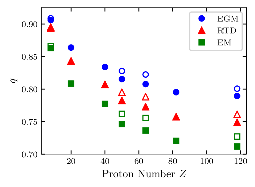
Figure 1: Total quenching trends with proton number for the different sets of LECs in Table 1, with $\bar{c}_{D}=0$. The solid symbols correspond to the lightest isotope of a given element and the open symbols to the heaviest one at the drip line.

Figure 1 shows the value of $q$ for all the nuclei in our data set except those in the middle of the isotopic chains. Because we use a density functional with no direct connection to the interactions and operators of $\chi$EFT, we consider three different sets of LECs for the long-range contribution to the current (see Table 1) and at first ignore the contact coefficient $\bar{c}_{D}$. We find that the two-body current always has an overall quenching effect. For all LEC sets, the amount of quenching increases with proton number, leading to values of $q$ between 0.86 and 0.91 in ²⁰O and between 0.73 and 0.80 in ³⁸⁸Og. For elements at the boundaries of the isotopic chain, we also observe slightly less quenching in the heavier isotopes than the lighter ones. The differences in $q$ between ²⁰O and ²⁸O are only $0.0014$–$0.0023$, however, while the differences between the heaviest and lightest isotopes for Sn, Gd, and Og are all larger and similar, averaging $0.013$–$0.017$.

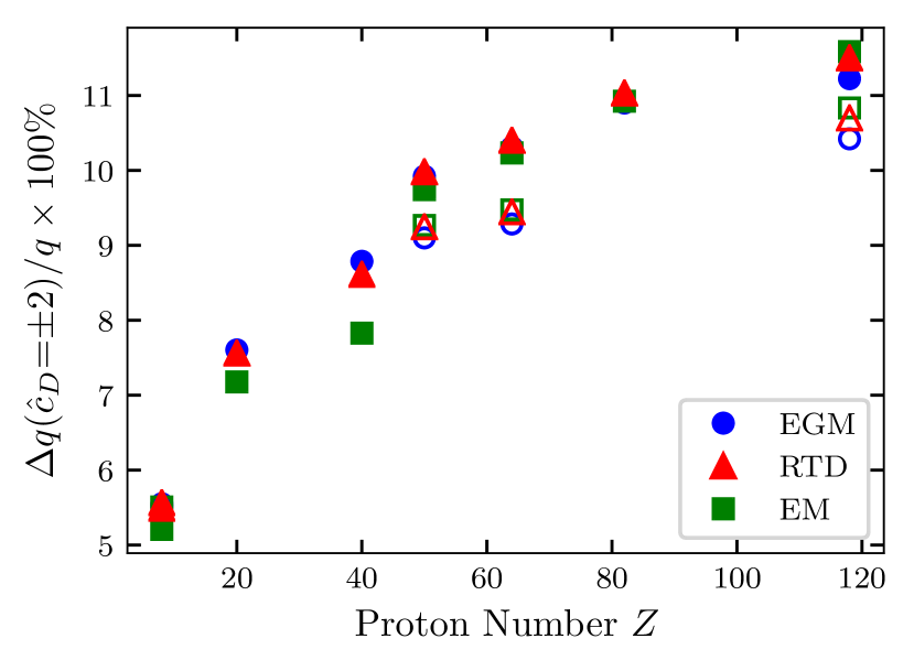
Figure 2: Same as Fig. 1 but for the change in $q$ with $\bar{c}_{D}=\pm 2$.

In Fig. 2 we examine the effect of the contact term. Equation (18) shows that adding a positive $\bar{c}_{D}$ reduces the quenching while adding a negative $\bar{c}_{D}$ increases it. The amount by which $q$ is raised or lowered is almost symmetric about $\bar{c}_{D}=0$, so the difference between the $\bar{c}_{D}=\pm 2$ values in Fig. 2 (denoted $\Delta q(\bar{c}_{D}=\pm 2)$) can be thought of as the size of error bars on the $q$ values in Fig. 1 due to the variation of $\bar{c}_{D}$ in this range. The $\bar{c}_{D}$ contribution by itself is the same for all LEC sets; small differences in its effects reflect the interference of the contact with the finite-range term. The size of the variation due to $\bar{c}_{D}$ follows the same trends with $N$ and $Z$ as $q$ itself, and ranges from $5\%$ to $10\%$ of $q$ at $\bar{c}_{D}=0$.

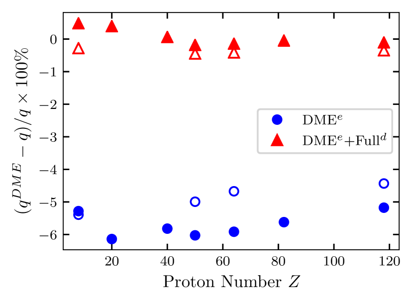
Figure 3: The difference between the total quenching produced by the density-matrix expansion (DME) and by the full calculation, as a percentage of the full quenching with the RTD parameter set Rentmeester et al. (2003). The blue circles correspond to predictions of the DME exchange current, not supplemented by anything else, while red triangles correspond to a supplementation of the DME exchange current by the full direct current (see text).

We compare calculations with the full current to those with the DME current in Fig. 3. The DME predictions — the circles in the figure — differ from those of the full current by roughly the same amount, $\sim 5\%$, for all nuclei. This indicates that the DME captures the same trends as in Fig. 1, but for all nuclei it overestimates the quenching slightly. The source of this discrepancy is the direct term, which is neglected in the DME. The squares in the figure add the full current’s direct term to the DME exchange term, producing a small correction that makes the agreement with the exact results almost perfect.

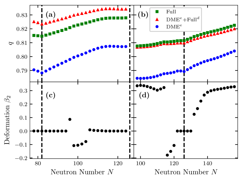
Figure 4: Total quenching in (a) Sn and (b) Gd isotopic chains using the EGM LEC set with the full current and the same versions of the DME shown in Fig. 3. (c) and (d) show the respective deformations. Vertical lines indicate the magic numbers $N=82$ and $126$.

Next, we explore trends with deformation and neutron excess by computing the two-body contributions for all even-even isotopes of Sn and Gd from $N=78$ to $N=124$ (Sn) and $N=98$ to $N=122$ (Gd). We use the EGM LEC set with $\bar{c}_{D}=0$, and again compare the full results with those of the DME. From Fig. 4(c) we see that the Sn nuclei are mostly spherical, though those in the middle of the shell are slightly deformed. On the other hand, Fig. 4(d) shows the Gd isotopes are very prolate, except right around the shell closure at $N=126$. Although we see a small increase in quenching near the shell closures in both elements, there is no significant trend with deformation. There is, however, a small, continuous decrease in quenching with neutron excess that is also apparent in Fig. 1. The DME exchange term mirrors the full calculation, again slightly overestimating the quenching. We display its results because they are so much easier to compute than the full results. Like the nuclear-matter approximation of Refs. Klos et al. (2013); Menéndez et al. (2011), the DME exchange expresses the two-body contribution as a density-dependent renormalization of the one-body Gamow-Teller operator. We thus expect the amount quenching to closely mirror the nuclear density.

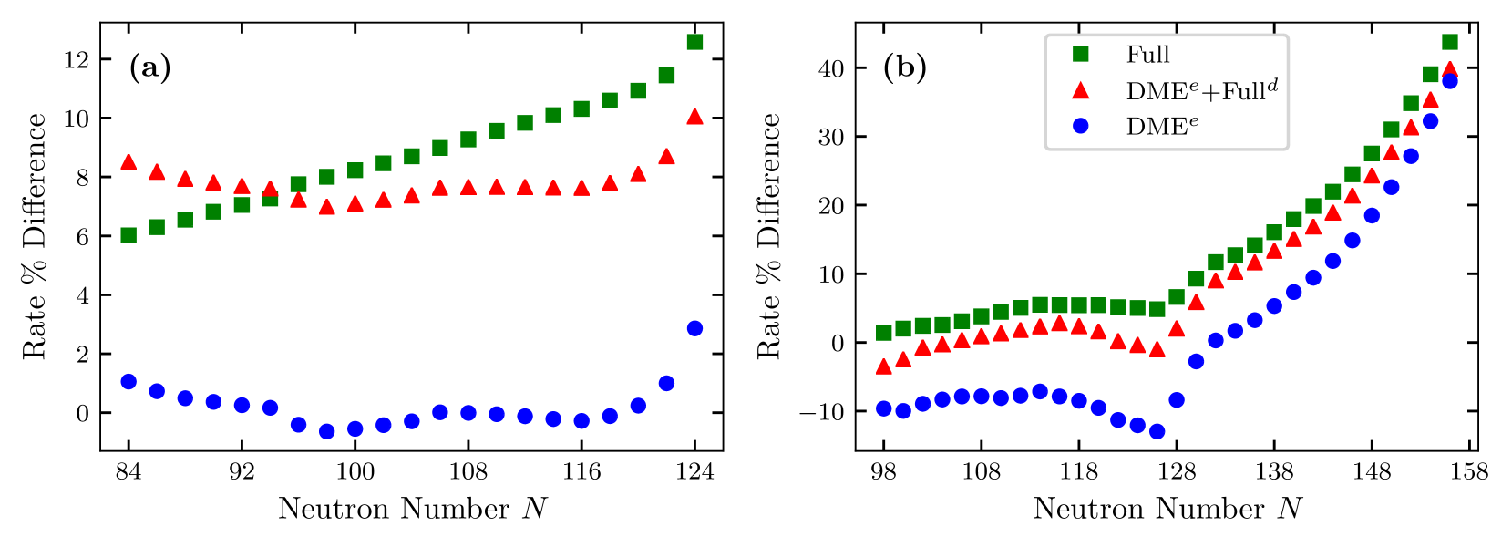
Figure 5: Comparison of Gamow-Teller rates computed with the full one-plus-two-body current and $g_{A}=1.27$ to those computed with the one-body current only and $g_{A}^{\text{eff}}=1.0$, in (a) Sn and (b) Gd isotopes. The percent difference is $(\lambda^{\text{1b+2b}}_{g_{A}=1.27}-\lambda^{\text{1b}}_{g_{A}=1.0})/\lambda^{\text{1b}}_{g_{A}=1.0}\times 100\%$, with $\lambda$ representing decay rates. The isotopes ¹²⁸Sn–¹³²Sn are excluded because the Gamow-Teller strength below the $\beta$-decay threshold is negligible.

IV.2 Gamow-Teller rates

We turn now to $\beta$-decay rates. They have been measured in only a few of the nuclei in our set and with the Skyrme functional that we use, we under-predict those rates even without including a two-body current Ney et al. (2020). We are thus not able to see how much the two-body current will improve the description of rates without re-calibrating the functional, perhaps even treating the LECs as free parameters, and examining more data. We leave that major task for a future publication. Here, however, we can still get an idea of what to expect by looking at the differences between rates computed with the one-body axial current and an effective axial-vector coupling $g_{A}^{\text{eff}}=1.0$, employed in most EDF work so far (including Ref. Ney et al. (2020)), and those computed with the one-plus-two-body axial current and the bare axial-vector coupling, $g_{A}=1.27$. To what extent does a nucleus- and energy-independent effective $g_{A}$ compensate for the omission of two-body currents?

We address the question in the Sn and Gd chains in Fig. 5, finding that in lighter isotopes the effective axial-vector coupling closely approximates the two-body current’s effect on the rate. In very neutron-rich nuclei, however, we begin to see a more significant difference between the two approaches. The Sn isotopes show a steady increase in the difference with neutron number, with an uptick near the drip line to about $12\%$. In the lighter Gd isotopes, the difference is very small until the $N=126$ shell closure, after which it increases markedly, to about $40\%$ in ²²⁰Gd. Although we do not plot the results, we have made the same rate comparison for the O and Og isotopes in our data set. In ²⁰O, the difference between the quenched one-body and unquenched one-plus-two-body rates is $32\%$ and in ²⁸O it is $24\%$, a variation of only about $8\%$. But in ³²²Og, the difference is $30\%$ and in ³⁸⁸Og it is $121\%$, a variation of over $90\%$. These findings suggest that a constant effective axial-vector coupling does not adequately account for the effects of two-body currents, particularly in very neutron-rich nuclei.

To understand the source of the discrepancy in neutron-rich isotopes, we examine the change in the low-lying one-body Gamow-Teller strength distributions (up to the $\beta$-decay threshold energy) caused by the two-body current for the lightest and heaviest Sn and Gd isotopes. This analysis is not so easy, unfortunately. The FAM requires that the strength distribution be computed with an artificial Lorentzian width applied to each transition, but the overlap of the Lorentzian tails from all transitions, in particular from the Gamow-Teller resonance, prevents us from using the strength for any one transition to compute the quenching factor for that transition. To get the best picture, we should use a very small artificial width to minimize the distortion. The FAM does not converge well close to the real axis, however, so we use a moderately small half-width of $\gamma=0.1$ MeV to maintain sufficient numerical stability.

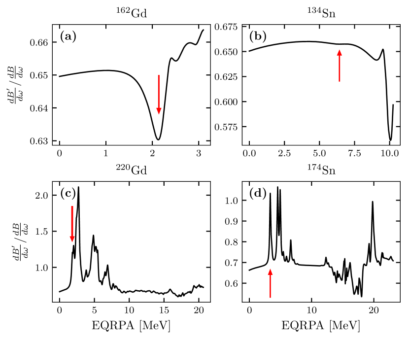
Figure 6: Ratio of the one-plus-two-body FAM strength to the one-body strength for low Gamow-Teller transition below the $\beta$-decay threshold energy in the light isotopes (a) ¹⁶²Gd and (b) ¹³⁴Sn, as well as the heavy isotopes (c) ²²⁰Gd and (d) ¹⁷⁴Sn. Arrows indicate the transitions examined in Figs. 7 and 8.

Figure 6 shows the resulting ratio of the one-plus-two-body strength to the one-body strength. The two-body current appears to affect all low-lying transitions in lighter isotopes in almost the same way, but in the heavier isotopes it appears to enhance some transitions. Such enhancement offsets the quenching of other transitions in the computation of $q$, explaining the significant underestimate made by the effective axial-vector coupling in these heavier nuclei.

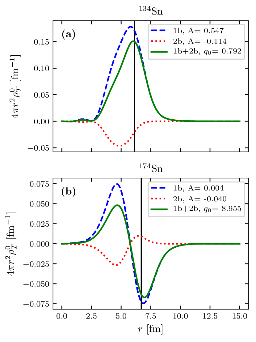
Figure 7: Density of the lowest lying Gamow-Teller transition amplitude in (a) ¹³⁴Sn and (b) ¹⁷⁴Sn as a function of the radial coordinate $r$. The curves show densities for the one-body, two-body, and one-plus-two-body amplitudes. The factor of $4\pi r^{2}$ makes the integrated amplitudes equal to the areas under the curves. The vertical line is at the spherical radius $R_{0}=1.2A^{1/3}$, and the legends show the amplitudes $A$ and quenching factors $q_{0}$ for the state in question. The overall signs of the amplitudes are arbitrary, but the relative signs between the one- and two-body terms are not. The quenching factor $q_{0}$ contains the square root of the squared amplitudes and is always positive.

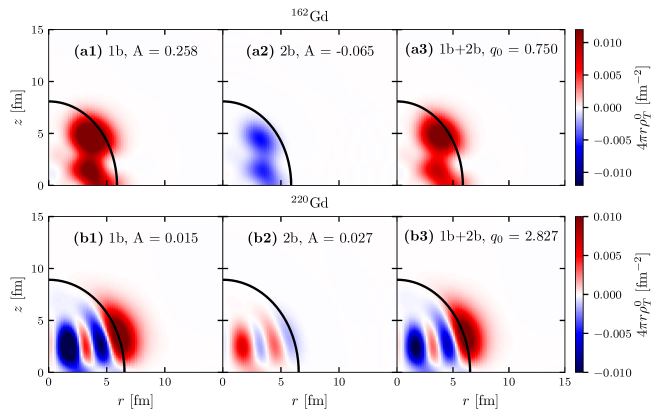
Figure 8: Density of the lowest lying Gamow-Teller transition amplitude in (a) ¹⁶²Gd and (b) ²²⁰Gd as a function of $r$ and $z$. The figures show densities for the (a1,b1) one-body, (a2,b2) two-body, and (a3,b3) one-plus-two-body amplitudes. The volume element of $4\pi r$ is included (with an extra factor of $2$ to account for the lower hemisphere). The curved lines indicate the nuclear surface determined from Eq. (38), with $r=1.2A^{1/3}$. The titles show the amplitudes $A$ and quenching factors $q_{0}$ for the state.

What causes the enhancement of some low-lying transitions in neutron-rich isotopes? To answer, we compute the transition-amplitude density for the lowest lying states in the heaviest and lightest Sn isotopes with non-negligible rates. Although the quenching discrepancy in the Sn rates is not as large as in that in the Gd rates, the Sn isotopes are easier to understand because they are mostly spherical, allowing us to display the density as a function of a single variable. We use the DME to compute the densities because it provides a local one-body external field, while the field from the full current is non-local. (Details on the computation of transition densities in the FAM appear in Appendix B.) Figure 7 shows that the two-body current contributes very little at or beyond the nuclear surface. The reason is the nucleon-density dependence in Eq. (20) of the DME current field, which weakens quickly as the density falls. The fall-off of the one-body curve is much slower. When the one-body contribution at the surface has the same sign as that in the interior, as in Fig. 7(a), this fact is not important and the two-body contribution quenches the transition amplitude. But when it has the opposite sign, leading to relatively small one-body transition strength, the difference between the quenching effect of the two-body current in the interior and its almost negligible effect at the surface causes the integrated matrix element to change sign and have a larger absolute value than without the two-body contribution, resulting in an enhanced strength.

As we already noted, enhancement is more common in neutron-rich nuclei than in those closer to stability. Although a careful and systematic analysis would be necessary to convincingly identify the physics responsible for the trend, the presence of a node in the transition-amplitude density associated with the space-independent operator $\bm{\sigma}t_{-}$ — the condition that leads to enhancement by the two-body current — implies a mismatch between the shapes of neutron and proton single-particle wave functions with the same spatial quantum numbers. Such a mismatch is much more common in isotopes with a large neutron excess.

Most of the Gd isotopes are deformed, and an analysis of transition-amplitude densities is more complicated than in Sn because the density is not constant on spherical shells. Nevertheless, we can proceed. Figure 8 shows the density for a slice of the upper right quadrant of the nuclei, and we see that these deformed isotopes exhibit the same phenomena as the Sn isotopes: quenching when the one-body density has the same sign everywhere and enhancement when it changes sign, because of a smaller two-body contribution at the surface than in the interior. In the heavier isotope here, however, the surface contribution outweighs the interior contribution even at the one-body level. The concentration of the two-body contribution, with opposite sign, in the interior, makes the imbalance even larger and enhances the integrated transition strength.

Although in this exploratory paper we are not yet examining the consequences of the energy- and isospin-dependence of the quenching for total $\beta$-decay rates, our findings suggest that they will be significant.

V Conclusions

We have developed a method to include the contributions of two-body charge-changing axial currents in the Skyrme-EDF linear-response, and applied the method to Gamow-Teller strength and $\beta$-decay rates. From the current, we construct mean-field-like external-field matrices that can easily be included in the linear response equations, e.g., through our charge-changing FAM. We have also developed a density matrix expansion for the two-body axial current. At leading order the expansion reproduces the contact current operator exactly and replaces the finite-range operator with a density-dependent one-body Gamow-Teller operator. This approximation reproduces the full linear response quite well for all the nuclei we studied, and provides a cheap way of including two-body contributions. If the direct term is computed exactly, an easier task in some codes than in our oscillator-based FAM, the expansion works almost perfectly.

To examine the effects on observables, we took the two-body current operators and the parameters that multiply them from $\chi$EFT. We found, first, that in all the nuclei we studied the two-body current quenches the summed Gamow-Teller strength. The quenching increases significantly with $Z$ and decreases with $N$. These trends can be understood by the density dependence of the effective one-body operator produced by the density-matrix expansion. We also looked at the energy dependence of the Gamow-Teller strength, finding that the two-body current causes a nearly constant quenching of decay to low-lying states near stability but a quenching with significant state dependence and in some cases even enhancement in very neutron-rich nuclei. Even though the amount of quenching of the summed strength changes just a little as $N$ grows, the enhancement of low-lying strength can cause $\beta$-decay rates to differ significantly from what would be predicted by a single effective $g_{A}$. The energy dependence in neutron-rich nuclei, like the isospin dependence of the quenching of summed strength, is connected with nuclear density profiles and the occurrence of zeroes in the spatial transition-amplitude distribution when the neutron excess is large.

Our results open up a number of interesting paths for future projects. Global calculations Ney et al. (2020); Mustonen and Engel (2016); Marketin et al. (2016); Möller et al. (2003) indicate that first-forbidden $\beta$ decay should be important in many nuclei, and our work should be extended to that channel and then applied to produce global calculations for $r$-process simulations. But most important is the marriage of $\chi$EFT with EDF theory. We have taken the first step here by including a chiral current together with a phenomenological density functional, in a way that is obviously not self consistent. It would make sense to refit not only the coupling constants of the functional but also the LECs in the currents. Once at least some of that is done, better systematic calculations of $\beta$-decay rates over the entire isotopic chart will become possible. Here the DME, which has already been applied to derive EDFs from chiral potentials Navarro Pérez et al. (2018); Navarro Pérez and Schunck (2019) and has been used to obtain an analogous density-dependent current, will be especially useful. And with existing computational technology, one might be able work directly with two-and three-body chiral interactions and currents, without the DME. The combination of EDF phenomenology and methods with ab initio interactions and currents is promising and should be fully investigated.

Appendix A Density matrix expansion

Although one might start from a time-dependent energy-density functional that includes the effects of currents, the result of a DME will be the same as if we we start with the “mean-field currents” $\widetilde{\bm{\Gamma}}_{\pi}$ and $\widetilde{\bm{\Gamma}}_{s}$. Instead of working with the charge-changing density, as we would in an energy functional, we (equivalently) obtain the DME exchange functional by applying Eq. (24) from Ref. Gebremariam et al. (2010) directly to the products of single-particle wave functions (those corresponding to the single particle states $i$ and $j$ in, e.g., Eq. (12)) as well as to densities. Using the 4-component spin-isospin vector $\Psi_{i}(\bm{r})$ in place of the individual components $\varphi_{i}(\bm{r},\sigma,\tau)$, we have

$$\Psi_{i}^{{\dagger}}(\bm{r}_{1})\Psi_{j}(\bm{r}_{2})=e^{i\bm{r}\cdot\bm{k}}e^{\bm{r}\cdot\left[\frac{1}{2}(\nabla_{1}-\nabla_{2})-i\bm{k}\right]}\Psi_{i}^{{\dagger}}(\bm{r}_{1})\Psi_{j}(\bm{r}_{2})\Big{|}_{\bm{r}_{1}=\bm{r}_{2}=\bm{R}}$$ (24)

$$\simeq e^{i\bm{r}\cdot\bm{k}}\left\{1+\bm{r}\cdot\left[\frac{1}{2}(\nabla_{1}-\nabla_{2})-i\bm{k}\right]+\frac{1}{2}\left(\bm{r}\cdot\left[\frac{1}{2}(\nabla_{1}-\nabla_{2})-i\bm{k}\right]\right)^{2}\right\}\Psi_{i}^{{\dagger}}(\bm{r}_{1})\Psi_{j}(\bm{r}_{2})\Big{|}_{\bm{r}_{1}=\bm{r}_{2}=\bm{R}}\,.$$

Here $\bm{k}$ is a characteristic momentum, $\bm{r}\equiv\bm{r}_{1}-\bm{r}_{2}$, and $\bm{R}\equiv\tfrac{1}{2}(\bm{r}_{1}+\bm{r}_{2})$.

For the decaying nucleon labeled by $i$ and $j$, we take the characteristic momentum to have magnitude $k_{F}$. Assuming that the decaying nucleon is near the Fermi surface, working at the leading-order in Eq. (24) for the decaying-nucleon states $\ket{i}$ and $\ket{j}$ – that is, neglecting all terms in the large braces except “1,” – and averaging over angles for the momenta $\bm{k}$ (with the assumption that the system is spherically symmetric) gives

$$\Psi_{i}^{{\dagger}}(\bm{r}_{1})\Psi_{j}(\bm{r}_{2})\longrightarrow\Pi_{1}^{s}\left[k_{F}(\bm{R})r\right]\Psi_{i}^{\dagger}(\bm{R})\Psi_{j}(\bm{R})\,,$$ (25)

with $\Pi_{1}^{s}[kr]\equiv j_{0}(kr)$ Gebremariam et al. (2010). For the nucleon densities associated with $\varphi_{k}$ and $\varphi_{l}$ in Eq. (12), we use the expansion expressions from Ref. Gebremariam et al. (2010). If, as for the full current, we neglect the terms in Eq. (7) that contain $\bm{p}_{1}$ and $\bm{p}_{2}$, the non-local spin density does not contribute and integrating the chiral current together with $\Pi_{1}^{s}\left[k_{F}(\bm{R})r\right]$ and the nucleon density from Eq. (26) of Ref. Gebremariam et al. (2010) over the relative coordinate $\bm{r}$ eliminates many of the other terms in Eq. (7). The integrals, together with the replacement of $\bm{R}$ by the one-body coordinate $\bm{r}$, result in Eq. (17). The expansion can be continued to higher order in both the wave functions of the decaying nucleon and the densities associated with the other nucleons, but we do not present the results of that analysis here.

The direct part of the current can also be expanded in the manner described in Ref. Dobaczewski et al. (2010), where it was applied to the Gogny interaction. When used together with the chiral interaction, however, the expansion does not converge quickly, at least in our tests. We attribute the problems to the long range of pion exchange. In any event, in leading order the direct current does not contribute at all, so that the most of the effects of the two-body currents come from the exchange current.

Appendix B Transition densities

We wish to understand why the two-body current quenches some low-lying transitions and enhances others, particularly in neutron-rich nuclei. To do so, we compute the spatial density of the transition amplitude for particular transitions. A transition amplitude to a given state within the FAM depends on the corresponding QRPA eigenvector, which we must extract. Once we have it, we obtain the transition amplitude from

$$\bra{m}F\ket{0}=\sum_{\mu<\nu}\big{(}X^{m*}_{\mu\nu}F^{20}_{\mu\nu}+Y^{m*}_{\mu\nu}F^{02}_{\mu\nu}\big{)}\,,$$ (26)

where the $X$’s and $Y$’s make up the QRPA eigenvector for state $\ket{m}$.

Reference Hinohara et al. (2013) explains how the QRPA modes are related to the FAM response and shows that they can be determined up to an unknown phase $e^{i\theta}={\bra{m}\hat{F}\ket{0}}/{\lvert\bra{m}\hat{F}\ket{0}}\rvert$, from the expression

$$X^{m}_{\mu\nu}=e^{i\theta}\ \frac{\text{Res}[X^{\text{FAM}},\Omega_{m}]}{\sqrt{\text{Res}[S,\Omega_{m}]}},\ Y^{m}_{\mu\nu}=e^{i\theta}\ \frac{\text{Res}[Y^{\text{FAM}},\Omega_{m}]}{\sqrt{\text{Res}[S,\Omega_{m}]}}\,,$$ (27)

where $\Omega_{m}$ is the excitation energy of state $\ket{m}$, $X^{\text{FAM}}$ and $Y^{\text{FAM}}$ are the FAM amplitudes Avogadro and Nakatsukasa (2011), $S$ is the FAM response given, e.g., in Eq. (28) of Ref. Hinohara et al. (2013), and $\text{Res}[A,\Omega_{m}]$ is the residue of quantity $A$ at frequency $\Omega_{m}$. One can extract the residues of the FAM quantities from contour integrals, but it is difficult to choose a contour that contains only a single transition. A more efficient but more approximate method to extract the residues is to compute the FAM quantities a small distance $\gamma$ above the real axis. The residue of $S$ is then given by Litvinova et al. (2007)

$$\text{Res}[S,\Omega_{m}]\approx-\gamma\mathrm{Im}[S(\Omega_{m}+i\gamma)]\,.$$ (28)

A similar relation holds for $X^{\text{FAM}}$ and $Y^{\text{FAM}}$ if we choose the undetermined phase such that the QRPA eigenvectors are real. To verify that the energy at which we are evaluating these functions is indeed a QRPA eigenvalue, and that the peak is well-separated enough for the approximation in Eq. (28) to hold, we compute the norm of the QRPA mode we extract:

$$N=\sum_{\mu<\nu}\big{(}X^{m*}_{\mu\nu}X^{m}_{\mu\nu}-Y^{m*}_{\mu\nu}Y^{m}_{\mu\nu}\big{)}\,.$$ (29)

If $N$ is close to one, we can be confident the results are close to the true QRPA values. The transitions highlighted in Fig. 6 all have values of $N>0.99$ for $\gamma=0.01$ MeV.

To obtain a spatial density for the transition amplitude we express Eq. (26) in coordinate space. Because the mean fields for one-body and two-body currents are one-body operators, they have the simple form

$$\hat{F}=\sum_{ij}f^{11}_{ij}a^{\dagger}_{i}a_{j}\,,$$ (30)

and the (charge-changing) transition-amplitude density can be defined through the relation

$$\bra{m}\hat{F}\ket{0}=\int d^{3}r\,\rho_{T}^{m}(\bm{r})\,,$$ (31)

where, for $\beta^{-}$ transitions,

$$\rho_{T}^{m}(r)=\sum_{\sigma,\sigma^{\prime}}\int d^{3}r^{\prime}\,\delta\rho^{m}(\bm{r}\sigma p,\bm{r}^{\prime}\sigma^{\prime}n)f^{11}(\bm{r}\sigma p,\bm{r}^{\prime}\sigma^{\prime}n)\,.$$ (32)

In Eq. (32) the term $\delta\rho^{m}$ is the density perturbation for the $m^{\text{th}}$ QRPA mode in coordinate space, obtained through a change of basis,

$$\delta\rho^{m}(\bm{r}\sigma p,\bm{r}^{\prime}\sigma^{\prime}n)=\sum_{pn}\phi_{p}^{*}(\bm{r}^{\prime}\sigma^{\prime}p)\phi_{n}(\bm{r}\sigma n)\delta\rho^{m}_{pn}\,,$$ (33)

where the $\phi_{k}(\bm{r}\sigma\tau)\equiv\psi^{\absolutevalue{\Lambda}}_{n_{r}n_{z}}(r,z)\frac{e^{i\Lambda\phi}}{\sqrt{2\pi}}\chi_{{}_{\Sigma}}(\sigma)\chi_{q}(\tau)$ are axially-deformed oscillator basis states and the $\delta\rho^{m}_{pn}$ are given by the inverse Bogoliubov transformation,

$$\delta\rho^{m}_{pn}=U_{p\pi}X^{m}_{\pi\nu}V^{T}_{n\nu}-V^{*}_{p\pi}Y^{m}_{\pi\nu}U^{\dagger}_{n\nu}\,,$$ (34)

where $U_{p\pi}$ refers to the $p^{\rm th}$ basis component of the $\pi^{\rm th}$ proton quasiparticle state and $U^{\dagger}_{n\nu}$ refers to the $n^{\rm th}$ basis component of the $\nu^{\rm th}$ neutron quasiparticle state.

The full two-body current is non-local in position space, so we use the DME approximation to get a transition-amplitude density that depends on the local particle density. We then define a density-dependent function $g[\rho]$ such that the one-, two-, and one-plus-two-body current external fields can all be written in the form

$$f^{11}(\bm{r}\sigma\tau,\bm{r}^{\prime}\sigma^{\prime}\tau^{\prime})=g[\rho(\bm{r})]\ \delta(\bm{r}-\bm{r}^{\prime})\\ \times\bra{\sigma}\bm{\sigma}\ket{\sigma^{\prime}}\bra{\tau}t_{-}\ket{\tau^{\prime}}$$ (35)

with

$$g[\rho(\bm{r})]=\begin{cases}-1&\text{one-body}\\ f[\rho(\bm{r})]&\text{two-body}\\ -1+f[\rho(\bm{r})]&\text{one-plus-two-body}\,,\end{cases}$$ (36)

and $f[\rho]$ the density-dependent function in Eq. (20).

Inserting Eqs. (33) and (35) into Eq. (32) we obtain the transition-amplitude density in our axially-deformed oscillator basis:

$$\rho_{T}^{m}(\bm{r})=g[\rho(\bm{r})]\sum_{pn}\delta\rho_{pn}^{m}\psi_{p}(r,z)\psi_{n}(r,z)\\ \times\bra{\sigma_{p}}\bm{\sigma}\ket{\sigma_{n}}\delta_{\Lambda_{p}\Lambda_{n}}\,.$$ (37)

The angular parts of the oscillator wave functions cause terms for which $\Lambda_{p}\neq\Lambda_{n}$ to vanish, so we have replaced them with a Kronecker delta to make the density real.

Finally, to construct radial plots for the two-dimensional axially-symmetric density, we can average the density over shells defined by a spherical radius ${r}$ and the deformation $\beta_{2}$,

$$S(r,\theta)=r\left[e^{-\frac{1}{2}\beta_{2}\sqrt{\frac{5}{4\pi}}}\cos(\theta)+e^{+\beta_{2}\sqrt{\frac{5}{4\pi}}}\sin(\theta)\right]\,.$$ (38)

For spherical nuclei $\beta_{2}=0$, so the surfaces becomes spheres and the value of the density over the surfaces is constant.

References

- Stuewer (1995) R. H. Stuewer, “The seventh solvay conference: Nuclear physics at the crossroads,” in No Truth Except in the Details: Essays in Honor of Martin J. Klein, edited by A. J. Kox and D. M. Siegel (Springer Netherlands, Dordrecht, 1995) pp. 333–362.
- Brown and Wildenthal (1988) B. A. Brown and B. H. Wildenthal, Annu. Rev. Nucl. Part. Sci. 38, 29 (1988).
- Chou et al. (1993) W.-T. Chou, E. K. Warburton, and B. A. Brown, Phys. Rev. C 47, 163 (1993).
- Martínez-Pinedo et al. (1996) G. Martínez-Pinedo, A. Poves, E. Caurier, and A. P. Zuker, Phys. Rev. C 53, R2602 (1996).
- Kumar et al. (2016) V. Kumar, P. C. Srivastava, and H. Li, J. Phys. G: Nucl. Part. Phys. 43, 105104 (2016).
- Suhonen (2017) J. T. Suhonen, Front. Phys. 5, 55 (2017).
- Engel and Menéndez (2017) J. Engel and J. Menéndez, Rep. Prog. Phys. 80, 046301 (2017).
- Gysbers et al. (2019) P. Gysbers, G. Hagen, J. D. Holt, G. R. Jansen, T. D. Morris, P. Navrátil, T. Papenbrock, S. Quaglioni, A. Schwenk, S. R. Stroberg, and K. A. Wendt, Nat. Phys. 15, 428 (2019).
- Menéndez et al. (2011) J. Menéndez, D. Gazit, and A. Schwenk, Phys. Rev. Lett. 107, 062501 (2011).
- Menéndez et al. (2012) J. Menéndez, D. Gazit, and A. Schwenk, Phys. Rev. D 86, 103511 (2012).
- Klos et al. (2013) P. Klos, J. Menéndez, D. Gazit, and A. Schwenk, Phys. Rev. D 88, 083516 (2013).
- Engel et al. (2014) J. Engel, F. Śimkovic, and P. Vogel, Phys. Rev. C 89, 64308 (2014).
- Hardy and Towner (2020) J. C. Hardy and I. S. Towner, Phys. Rev. C 102, 045501 (2020).
- Walecka (1975) J. Walecka, in Muon Phys. (Academic Press, Inc., 1975) Chap. 5, pp. 113–218.
- Zyla et al. (2020) P. Zyla et al. (Particle Data Group), Prog. Theor. Exp. Phys. 2020, 083C01 (2020).
- Park et al. (2003) T.-S. Park, L. E. Marcucci, R. Schiavilla, M. Viviani, A. Kievsky, S. Rosati, K. Kubodera, D.-P. Min, and M. Rho, Phys. Rev. C 67, 055206 (2003).
- Krebs et al. (2017) H. Krebs, E. Epelbaum, and U.-G. Meißner, Ann. Phys. (N. Y.) 378, 317 (2017).
- Wang et al. (2018) L.-J. Wang, J. Engel, and J. M. Yao, Phys. Rev. C 98, 031301(R) (2018).
- Ring and Schuck (2004) P. Ring and P. Schuck, The Nuclear Many-Body Problem (Springer, 2004).
- Nakatsukasa et al. (2007) T. Nakatsukasa, T. Inakura, and K. Yabana, Phys. Rev. C 76, 024318 (2007).
- Avogadro and Nakatsukasa (2011) P. Avogadro and T. Nakatsukasa, Phys. Rev. C 84, 014314 (2011).
- Mustonen et al. (2014) M. T. Mustonen, T. Shafer, Z. Zenginerler, and J. Engel, Phys. Rev. C 90, 024308 (2014).
- Shafer et al. (2016) T. Shafer, J. Engel, C. Frohlich, G. C. McLaughlin, M. Mumpower, and R. Surman, Phys. Rev. C 94, 055802 (2016).
- Ney et al. (2020) E. M. Ney, J. Engel, T. Li, and N. Schunck, Phys. Rev. C 102, 034326 (2020).
- Bohr and Mottelson (1998) A. Bohr and B. R. Mottelson, Nuclear Structure Volume II: Nuclear Deformations (World Scientific, 1998).
- Stoitsov et al. (2005) M. V. Stoitsov, J. Dobaczewski, W. Nazarewicz, and P. Ring, Comput. Phys. Commun. 167, 43 (2005).
- Stoitsov et al. (2013) M. V. Stoitsov, N. Schunck, M. Kortelainen, N. Michel, H. Nam, E. Olsen, J. Sarich, and S. Wild, Comput. Phys. Commun. 184, 1592 (2013).
- Navarro Pérez et al. (2017) R. Navarro Pérez, N. Schunck, R. D. Lasseri, C. Zhang, and J. Sarich, Comput. Phys. Commun. 220, 363 (2017).
- Mustonen and Engel (2016) M. T. Mustonen and J. Engel, Phys. Rev. C 93, 014304 (2016).
- Schunck (2019) N. Schunck, Energy Density Functional Methods for Atomic Nuclei (IOP Publishing, 2019).
- Perlińska et al. (2004) E. Perlińska, S. G. Rohoziński, J. Dobaczewski, and W. Nazarewicz, Phys. Rev. C 69, 014316 (2004).
- Parrish et al. (2013) R. M. Parrish, E. G. Hohenstein, N. F. Schunck, C. D. Sherrill, and T. J. Martínez, Phys. Rev. Lett. 111, 132505 (2013).
- Dobaczewski et al. (2009) J. Dobaczewski, W. Satuła, B. G. Carlsson, J. Engel, P. Olbratowski, P. Powałowski, M. Sadziak, J. Sarich, N. Schunck, A. Staszczak, M. Stoitsov, M. Zalewski, and H. Zdú Nczuk, Comput. Phys. Commun. 180, 2361 (2009).
- Younes (2009) W. Younes, Comput. Phys. Commun. 180, 1013 (2009).
- Negele and Vautherin (1972) J. W. Negele and D. Vautherin, Phys. Rev. C 5, 1472 (1972).
- Gebremariam et al. (2010) B. Gebremariam, T. Duguet, and S. K. Bogner, Phys. Rev. C 82, 014305 (2010).
- Bogner et al. (2011) S. K. Bogner, R. J. Furnstahl, H. Hergert, M. Kortelainen, P. Maris, M. Stoitsov, and J. P. Vary, Phys. Rev. C 84, 044306 (2011).
- Dyhdalo et al. (2017) A. Dyhdalo, S. K. Bogner, and R. J. Furnstahl, Phys. Rev. C 95, 054314 (2017).
- Navarro Pérez et al. (2018) R. Navarro Pérez, N. Schunck, A. Dyhdalo, R. J. Furnstahl, and S. K. Bogner, Phys. Rev. C 97, 054304 (2018).
- Dobaczewski et al. (2010) J. Dobaczewski, B. G. Carlsson, and M. Kortelainen, J. Phys. G: Nucl. Part. Phys. 37, 075106 (2010).
- Epelbaum et al. (2005) E. Epelbaum, W. Glöckle, and U.-G. Meißner, Nucl. Phys. A 747, 362 (2005).
- Rentmeester et al. (2003) M. C. M. Rentmeester, R. G. E. Timmermans, and J. J. de Swart, Phys. Rev. C 67, 044001 (2003).
- Entem and Machleidt (2003) D. R. Entem and R. Machleidt, Phys. Rev. C 68, 041001 (2003).
- Marketin et al. (2016) T. Marketin, L. Huther, and G. Martínez-Pinedo, Phys. Rev. C 93, 025805 (2016).
- Möller et al. (2003) P. Möller, B. Pfeiffer, and K.-L. Kratz, Phys. Rev. C 67, 055802 (2003).
- Navarro Pérez and Schunck (2019) R. Navarro Pérez and N. Schunck, J. Phys. Conf. Ser. 1308, 012014 (2019).
- Hinohara et al. (2013) N. Hinohara, M. Kortelainen, and W. Nazarewicz, Phys. Rev. C 87, 064309 (2013).
- Litvinova et al. (2007) E. Litvinova, P. Ring, and V. Tselyaev, Phys. Rev. C 75, 064308 (2007).