The Lévy Flight of Cities: Analyzing Social-Economical Trajectories with Auto-Embedding

Abstract

It has been found that human mobility exhibits random patterns following the Lévy flight, where human movement contains many short flights and some long flights, and these flights follow a power-law distribution. In this paper, we study the social-economical development trajectories of urban cities. We observe that social-economical movement of cities also exhibit the Lévy flight characteristics. We collect the social and economical data such as the population, the number of students, GDP and personal income, etc. from several cities. Then we map these urban data into the social and economical factors through a deep-learning embedding method Auto-Encoder. We find that the social-economical factors of these cities can be fitted approximately as a movement pattern of a power-law distribution. We use the Stochastic Multiplicative Processes (SMP) to explain such movement, where in the presence of a boundary constraint, the SMP leads to a power law distribution. It means that the social-economical trajectories of cities also follow a Lévy flight pattern, where some years have large changes in terms of social-economical development, and many years have little changes.

Research

Introduction

Urban studies seek to understand and explain regularities observed in the world’s major urban systems. Cities are complex systems [1, 2, 3, 4, 5, 6, 7, 8] with many people living in and complex relationships among various factors. Previous works have studied the mobility of people [9] and show that the movement of human society is statistically random. A lot of studies are about the rank-order of cities [10, 11, 12, 13, 3, 14], Pareto law [11, 15] and Zipf’s law [16, 4, 17]. In this paper, we study the development trajectories of cities to contribute to the sustainability and innovation of cities [2, 18, 19, 20, 18]. This paper will aid policymakers, city planners and government officials to understand the nature of urban development and design a sustainable smart cities using computational social science models.

In this paper, we follow the urban dynamics model above and assume that cities move in two directions [21]: one is economic growth, the other is the development of social civilization. We study the datasets of four Asian cities: two in China including Hong Kong and Shanghai, the third is Singapore, the fourth is Tokyo, Japan. (see Table 1) All of them have economic factors such as GDP, GDP of secondary industry and GDP of tertiary industry, and social factors such as population, education and publication. It covers the most commonly used data types for measuring urban development [10]. Firstly, it is clear that the research object is urban mobility [22], namely the change amount of urban economic and social development, and the change amount of social and economic factors is obtained. Then, we apply the recently popular artificial neural network embedding technique, namely Auto-Encoder [23], on all economic factors to extract a low-dimensional latent vector. Min-max normalization is performed on the data first, and the same was done on the data of social factors. Next, we determine the step size distribution of the city movement. According to Akaike Information Criterion [24], the distribution model is fitted to get the optimal probability distribution. The results show that the movement of Hong Kong is more in line with the truncated power law [25] distribution, Shanghai city and Tokyo move more power law, and Singapore moves in the pattern of exponential distribution. To the best of our knowledge, this article is the first work that examines the movement of urban social-economical developments using computational social science models and explain the generalization model behind it.

The contribution of this paper is as follows. First, we extract the increment distribution function of city’s society according to city’s economy. Second, we demonstrate that log-normal processes [26, 27, 28] in the presence of a boundary constraint, approximately yields a generative process with a power law distribution. This result is a step towards explaining the emergence of Lévy flight patterns in city development. Thirdly, we use the stochastic multiplicative processes [29, 30, 31, 32, 33, 34] to explain the urban development trajectory, regarding city as an organism growing theory [35].

Results

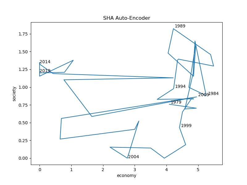
(b) SHA Auto-Encoder

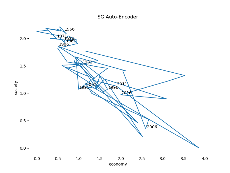
(c) SG Auto-encoder

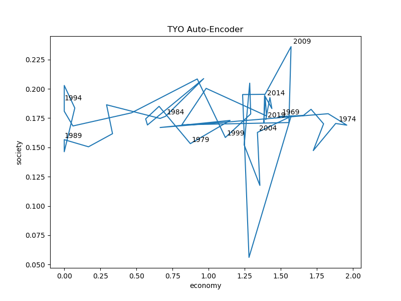
(d) TYO Auto-Encoder

Figure 1: Auto-Encoder The economical and social trajectory of urban development.As can be seen from the figure(a), before the opening up of the Pudong District in 1990, the development step size of Shanghai was relatively small.The 2010 Shanghai World Expo has led to a rapid economic development. As can be seen from the figure(b), after Hong Kong’s return to China in 1997, it enjoyed social and economical stability and prosperity, and successfully fended off the Asian financial crisis in 1998. After 2010, Hong Kong’s economic and social development was sluggish.

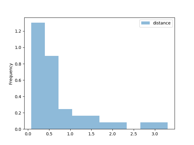
(a) HK histogram

(b) SHA histogram

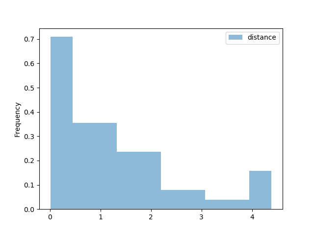
(c) SG histogram

(d) TYO histogram

Figure 2: Histogram of flight length.As can be seen from both the figure(a), (b), (c) and (d), all of the histograms are positive skewed. The statistical analysis of the step size of the random walk shows obvious ”heavy tail” feature, which satisfies the walking characteristics of frequent short-distance walk and occasional long-distance jump.

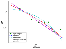
(a) HK Truncated power-law

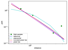
(b) SHA Power-law

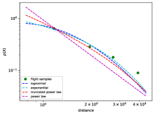
(c) SG Exponential

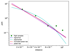
(d) TYO Power-law

Figure 3: Fitted distributions. Hong Kong has experienced rapid development and sharp decline. The urban development step size is relatively rich, with more long-distance jump. The fitted Truncated power-law distribution has a thicker tail, with alpha 1.3547. The development step size of Shanghai has more short-distance walk and less long-distance jump. It is still in a stable development period. The $\alpha$ of the fitted Power-law distribution is 2.2829. Singapore has been developing with relatively constant multiplicative factor, the fitted Exponential distribution with $\lambda=1.6075$. With the Exponential Transformation, the exponential distribution can deducted to Power-law distribution with $\alpha=1+\lambda=2.6075$. Tokyo has been developing relatively earlier than Shanghai, the fitted Power-law distribution has a larger $\alpha$ 2.6016.

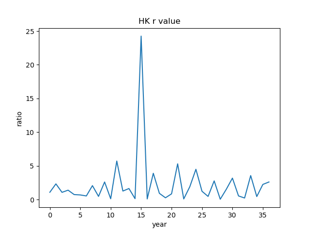
(a) HK r value

(b) SHA r value

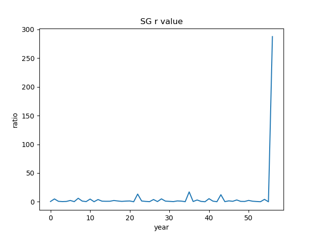
(c) SG r value

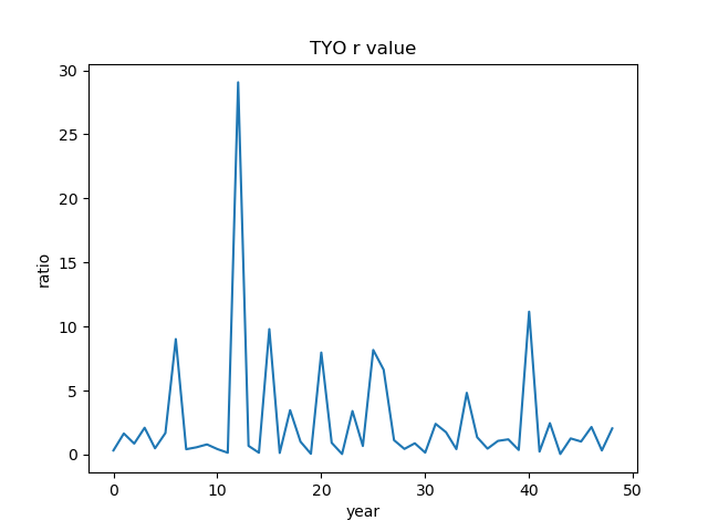
(d) TYO r value

Figure 4: The relative change rates. The change rate is defined as the relative change of length between two consecutive flights. From these figures we observe that the change rate are uncorrelated from one time interval to the other.

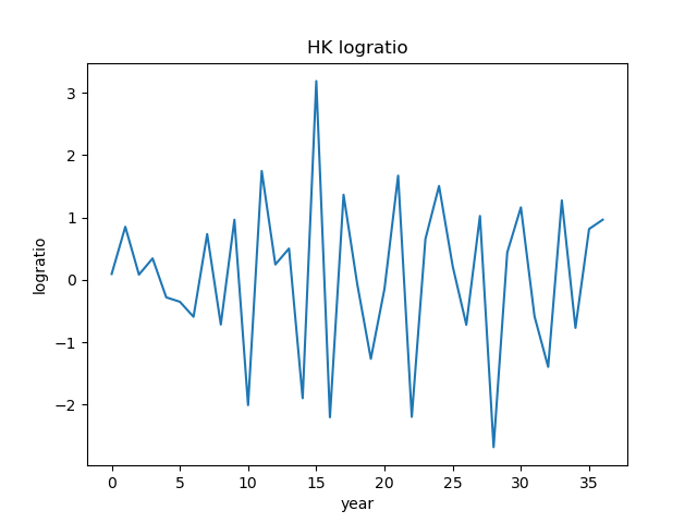
(a) HK $\ln r$ value

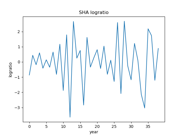
(b) SHA $\ln r$ value

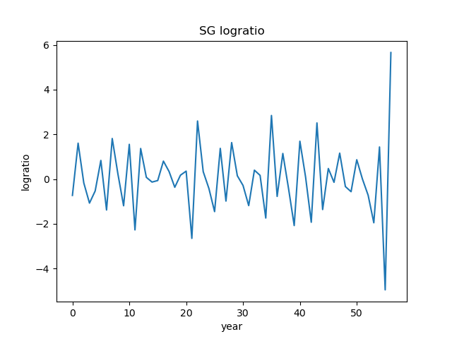
(c) SG $\ln r$ value

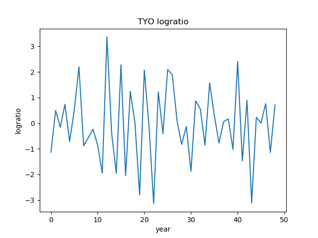
(d) TYO $\ln r$ value

Figure 5: $\ln r$ of four cities

Power-law fit for city trajectory flight. First, we draw the social-economical trajectories (see Figure 1) of cities and get the histograms (see Figure 2) of walk lengths. We fit the walk length distribution (see Figure 3) of the Shanghai city, the Hong Kong City, Singapore and the Tokyo city. We fit truncated power law [9], log-normal, power law [30, 26, 36, 25, 37], and exponential distribution [38]. (see Table 2) Then use Akaike weights (see Table 3) to choose the best fitted distribution. We find that the urban development step size of Hong Kong fits Truncated power-law distribution with $\alpha=1.3547$, and the walk distributions of the other three cities fit Power-law distributions. The exponent $\alpha$ is 2.2829 for Shanghai, 2.6075 for Singapore and 2.6016 for Tokyo. Assuming that urban development satisfy the stochastic multiplicative processes, we draw the walk length change rate (see Figure 4) and logarithm of change rate (see Figure 5). The deducted exponents $\alpha$ by SMP are similar to those of the fitted values of $\alpha$. (see Table 4)

Mechanisms behind the Power law pattern. A city should be considered an ever changing organism instead of a static one. At each step $t$, the organism may grow or shrink [2], according to a random variable $R_{t}$, so that the change of the city $l_{t}=r_{t-1}l_{t-1}$. This is stochastic multiplicative processes [31] $l_{t}=r_{t}r_{t-1}...r_{1}l_{0}$. The idea is that the random growth of an organism is expressed as a percentage of its current increment, and is independent of its current actual size. Then we find

$$\ln l_{t} = \sum_{i=1}^{t}\ln r_{i}+\ln l_{0}$$ (1)

Assuming the random variables $\ln R_{i}$ satisfy independent and identical distributions with mean $v$ and variance $D$, the Central Limit Theorem says that $\ln L_{t}=\sum_{i=1}^{t}\ln R_{i}+\ln l_{0}$ converges to a normal distribution with mean $vt$ and variance $Dt$ for sufficiently large $t$, which means $L_{t}$ converges to a log-normal distribution. In this paper, we use Kolmogorov-Smirnov test to verify that all the datasets $lnr$ of four cities can be reasonably assumed satisfy normal distributions (see Figure 5 and Table 5). Note here that $l_{t}$ is the length of the flight between time $t-1$ and time $t$. The probability density function of the flight length with the same change variable is log-normal.

$$f(l_{t}) = \frac{1}{\sqrt{2\pi Dt}}\frac{1}{l_{t}}exp\left[-\frac{1}{2Dt}(\ln l_{t}-vt)^{2}\right]$$ (2)

$$= \frac{1}{\sqrt{2\pi Dt}}l_{t}^{-1+\frac{v}{D}}exp\left[-\frac{1}{2Dt}(\ln^{2}l_{t}+v^{2}t^{2})\right]$$

Given

$$f(l_{t})=\frac{1}{l_{t}\sqrt{2\pi Dt}}exp[-\frac{(\ln l_{t}-vt)^{2}}{2Dt}]$$

$$=\frac{1}{l_{t}\sqrt{2\pi Dt}}exp[-\frac{(\ln l_{t})^{2}-2vt\ln l_{t}+v^{2}t^{2}}{2Dt}]$$

$$=\frac{1}{l_{t}\sqrt{2\pi Dt}}exp[-\frac{(\ln l_{t})^{2}+v^{2}t^{2}}{2Dt}]exp(\frac{v\ln l_{t}}{D})$$

$$=\frac{1}{l_{t}\sqrt{2\pi Dt}}l_{t}^{\frac{v}{D}}exp[-\frac{(\ln l_{t})^{2}+v^{2}t^{2}}{2Dt}]$$

$$=\frac{1}{\sqrt{2\pi Dt}}l_{t}^{-1+\frac{v}{D}}exp[-\frac{(\ln l_{t})^{2}+v^{2}t^{2}}{2Dt}]$$

This form shows that the log-normal distribution can be mistaken for an apparent power law. If $\sigma\to\infty$, then $\frac{(\ln l_{t})^{2}}{2Dt}\to 0$.

$$f(l_{t})\to\frac{1}{\sqrt{2\pi Dt}}exp[-\frac{v^{2}t}{2D}]l_{t}^{-1+\frac{v}{D}}\to Cl_{t}^{\alpha}$$

The Probability Density Function of log-normal distribution is indistinguishable from that of power law distribution $f(l_{t})=Cl_{t}^{-\alpha}$, where $1<\alpha\leq 3$.

If there exists a lower bound $l_{min}$,

$$l_{t}=max(l_{min},r_{t-1}l_{t-1})$$

then $L_{t}$ converges to a power law distribution, log-normal easily pushed to a power law model.

Here the $v$ and the $D$ are the normalized mean and variance of $\ln R$.

If there exists a lower bound $l_{min}$, such that $l_{t}=max(l_{min},r_{t-1}l_{t-1})$, then the random variable $L_{t}$ converges to a power law distribution, log-normal easily pushed to a power law model.

Discussion

Previous research suggests that power laws widely exist in city population, financial markets and city-size [11, 14]. However, the rank-size distribution between cities [13] is mostly static, The dynamic urban power-law distribution focuses on the change of specific indicators over time, while the systematic change [1] among urban factors has not been studied. By using a recently popular neural network embedding technique to reduce the dimension of urban factor data-sets into two dimensions: economy and society, we explore the city development trajectory of Hong kong, Shanghai, Singapore and Tokyo. The urban development of Hong Kong tends to be truncated power law distribution. This is probably because the rapid development of China’s reform and opening up has weakened Hong Kong’s status as an important city in Southeast Asia, and Hong Kong is no longer the uniquely preferred city in the allocation of various resources in China.

Methods

Data Sets. We collected the official data-sets of Hong kong (see Table 6), Shanghai (see Table 7), Singapore (see Table 8) and Tokyo (see Table 9) in our work, The data-sets of the four cities were collated and matched. Using the embedding technique to reduce the dimensions of those data-sets into two dimensions: economy and society. Then, we draw the urban development trajectory (see Figure 1) with economy as $x$-coordinates and society as $y$-coordinate. we extract the following information from the graph: flight lengths.

Obtaining Flight Length of each factor. To the best of our knowledge, this article is the first work that examines the flight length distribution of urban development. Firstly, we get raw data of each year’s flight length for each factor. The GDP factor ranges from dozens to thousands, while Proportion of industry ranges between 0 and 4, the range of values of raw data varies widely. To avoid the flight length being governed by large value data, we use min-max normalization to scale the range of each factor in [0, 1].

Obtaining Flight length of urban development by Embedding. The Manifold Hypothesis states that real-world high-dimensional data lie on low-dimensional manifolds embedded within the high-dimensional space. In this paper, we try to get embedding layer through training Auto-encoder (AE), which is a type of artificial neural network. Firstly, we classifies the data into two classes, for example, regarding GDP, per capita GDP and primary GDP as economic variables, regarding population and General higher education as social variables. Secondly, we use min-max scaling to make sure variables that are measured at different scales contribute equally to the model fitting. Thirdly, in the AE, the input feature,the dataset of economic variables or social variables, is transformed into one latent space with the encoder and then reconstructed from latent space with decoder. The encoder is used as a dimensionality reducer. To train this AE, an Adam algorithm was applied as an optimizer and mean square error (MSE) as a loss function. We use two-layer fully connected networks as the encoder and decoder, and the loss function is

$$\mathcal{L}(\textbf{x},\textbf{x}^{\prime}) = \left\|\textbf{x}-\textbf{x}^{\prime}\right\|^{2}$$ (3)

$$= \left\|\textbf{x}-f(h(\textbf{x}))\right\|^{2}$$

where $\textbf{x}\in\mathbb{R}^{n}$ is the input feature of one year and $n$ is the number of variables. The data from $m$ years construct $m$ training samples. $\textbf{x}^{\prime}$ is the output of the decoder. The computation of the encoder and decoder is defined as

$$h(\textbf{x}) = \sigma(W_{2}\sigma(W_{1}\textbf{x}+b_{1})+b_{2}),$$

$$f(\textbf{y}) = \sigma^{\prime}(W_{2}^{\prime}\sigma^{\prime}(W_{1}^{\prime}\textbf{y}+b_{1}^{\prime})+b_{2}^{\prime})$$ (4)

where $W_{1},W_{2},W_{1}^{\prime},W_{2}^{\prime},b_{1},b_{2},b_{1}^{\prime},b_{2}^{\prime}$ are learnable parameters of the network, and $\sigma,\sigma^{\prime}$ are the activation functions. We train the AE by minimizing the MSE of the input feature and the output of the decoder. And the output of the encoder $h(\mathbf{x})$ is the embedding of the original input.

Identifying the Scale Range. To fit a heavy tailed distribution such as a power law distribution, we need to determine what portion of the data to fit $x_{min}$ and the scaling parameter $\alpha$. We use the methods from [39] to determine $x_{min}$ and $\alpha$. We create a power law fit starting from each value in the dataset. Then we select the one that results in the minimal Kolmogorov-Smirnov distance between the data and the fit, as the optimal value of $x_{min}$. After that, the scaling parameter $\alpha$ in the power law distribution is given by

$$\alpha = 1+n\left(\sum_{i=1}^{n}\ln\frac{x_{i}}{x_{min}}\right)^{-1}$$ (5)

where $x_{i}$ are the observed values of $x_{i}>x_{min}$ and $n$ is the number of samples.

Exponential transformation The probability density function of exponential distribution can be transformed into power law distribution. Let $X$ be an exponential random variable whose probability density function is given by $P(X=x)=\lambda e^{-\lambda x},\lambda>0,x>0$, then the cumulative probability function is given by

$$P(X\leq x) = \int_{0}^{x}\lambda e^{-\lambda t}dt$$ (6)

$$= 1-e^{-\lambda x},\lambda>0,x>0$$

and let $Y$ be the random variable obtained through the transformation $Y=ke^{X}$, $k>0$, we can express the cumulative density function of $Y$ in terms of the cumulative density function of $X$ as

$$P(Y\leq y) = P(ke^{X}\leq y)$$

$$= P\left[X\leq\ln(\frac{y}{k})\right]$$

$$= 1-e^{-\lambda\ln(\frac{y}{k})}$$

$$= 1-(\frac{y}{k})^{-\lambda}$$

$$= 1-k^{\lambda}y^{-\lambda}$$

$$P(Y=y) = \lambda k^{\lambda}y^{-(1+\lambda)}$$ (7)

which corresponds to the Probability Density Function of the Power-law distribution with shape factor $\alpha=1+\lambda$.

Akaike weights. We use Akaike weights to choose the best fitted distribution. An Akaike weight is a normalized distribution selection criterion. Its value is between 0 and 1. A larger value indicates a better fitted distribution.

Akaike’s information criterion (AIC) is used in combination with Maximum likelihood estimation (MLE). MLE finds an estimator of $\hat{\theta}$ that maximizes the likelihood function $L(\hat{\theta}|data)$ of one distribution. AIC is used to describe the best fitting one among all fitted distributions,

$$AIC = -2log\left(L(\hat{\theta}|data)\right)+2K.$$ (8)

Here $K$ is the number of estimable parameters in the approximating model.

After determining the AIC value of each fitted distribution, we normalize these values as follows. First of all, we extract the difference between different AIC values called $\Delta_{i}$,

$$\Delta_{i} = AIC_{i}-AIC_{min}.$$ (9)

Then Akaike weights $W_{i}$ are calculated as follows,

$$W_{i} = \frac{exp(-\Delta_{i}/2)}{\sum_{r=1}^{R}exp(-\Delta_{i}/2)}.$$ (10)

The statistics can be see in Table 3.

A List of abbreviations

HK: Hong Kong

SHA: Shanghai

SG: Singapore

TYO: Tokyo

pdf: probability density function

SMP: Stochastic Multiplicative Processes

AE: Auto-encoder

MSE: mean square error

AIC: Akaike’s information criterion

MLE: maximum likelihood estimation

Availability of data and material

The data can be collected from official websites, which are listed in Table 6, Table 7, Table 8 and Table 9.

Funding

This work is partially supported by National Natural Science Foundation of China (Grant No. 61972286).

Competing interests

The authors declare that they have no competing interests.

Author’s contributions

Weixiong Rao and Kai Zhao conceived the experiments, Linfang Tian and Jiamin Yin conducted the experiments, Linfang Tian analysed the results. All authors reviewed the manuscript.

Figures and Tables

(a) HK Auto-Encoder

Table 1: The analysis of Hongkong, Shanghai, Singapore and Tokyo Datasets

Class	Description	HK	SHA	SG	TYO
Economy	GDP	1981-2019	1978-2018	1960-2019	1968-2019
	Primary industry	1981-2019	1978-2018	NA	NA
	Secondary industry	1981-2019	1978-2018	1960-2019	NA
	Tertiary industry	1981-2019	1978-2018	1960-2019	NA
	Share of Primary industry	1981-2019	1978-2018	NA	NA
	Share of Secondary industry	1981-2019	1978-2018	1960-2019	NA
	Share of Tertiary industry	1981-2019	1978-2018	1960-2019	NA
	Per capita GDP	1981-2019	1978-2018	NA	NA
	Government revenue	1981-2019	1978-2018	NA	NA
	Government expenditure	1981-2019	1978-2018	1960-2019	NA
	Personal income	NA	NA	NA	1960-2019
	Original insurance income	NA	1978-2018	NA	NA
	Original insurance pays out	NA	1978-2018	NA	NA
	Total fixed asset investment	NA	1978-2018	1960-2019	NA
	Industry	NA	1978-2018	1960-2019	1968-2019
	GDP per capita(Dollar)	NA	1978-2018	NA	NA
	Proportion of industry	NA	1978-2018	1960-2019	NA
	Gross agricultural production	NA	1978-2018	NA	NA
	Gross industrial production	NA	1978-2018	1960-2019	1968-2019
Society	Population	1981-2019	1978-2018	1960-2019	1968-2019
	Labor	NA	NA	NA	1968-2019
	General Tertiary education	1981-2019	1978-2018	1960-2019	1968-2019
	Ordinary secondary school	1981-2019	1978-2018	1960-2019	1968-2019
	Ordinary primary school	1981-2019	1978-2018	1960-2019	1968-2019
	Book print run	NA	1978-2018	NA	NA
	Journal print run	NA	1978-2018	NA	NA
	Newspaper print run	NA	1978-2018	NA	NA

Table 2: Fitted distributions. With $1<\alpha\leq 3$, the Power-law distribution has infinite variance. It has infinite mean as $1<\alpha\leq 2$ and finite mean as $2<\alpha\leq 3$.

Distribution	Probability density function (pdf)
Exponential	$\lambda e^{-\lambda x}$
Power-law	$Cx^{-\alpha}$
Lognormal	$\frac{1}{x\sigma\sqrt{2\pi}}exp[-\frac{(\ln(x)-\mu)^{2}}{2\sigma^{2}}]$
Truncated power-law	$Cx^{-\alpha}e^{-\gamma x}$

Table 3: Akaike weights of fitted distributions in the four cities datasets.

Cities	Exponential	Power-law	Lognormal	Truncated Power-law
HK	0.1979	0.2568	0.2226	0.3227
SHA	0.0401	0.4603	0.2163	0.2814
SG	0.6717	0.0014	0.1283	0.1985
TYO	0.1594	0.4132	0.1979	0.2295

Table 4: The calculated and estimated parameters for consecutive flights length in the four cities datasets, with $\ln R_{i}$ taken in the interval [0.48, 1.48][29]. The mean is noted as $v^{\prime}$, and variance is $D^{\prime}$, $\hat{\alpha}$ is calculated, and $\alpha$ is the fitted exponent. Here the walk lengths of Hong kong is fitted Truncated power-law rather than Power-law distribution.

Cities	$l_{min}$	$v^{\prime}$	$D^{\prime}$	$v^{\prime}/D^{\prime}$	$\hat{\alpha}$	$\alpha$
HK*	0.0752	-0.1904	0.1443	-1.3200	2.3200	1.3547
SHA	0.0216	-0.1010	0.0751	-1.3453	2.3453	2.2829
SG	0.0262	-0.1310	0.1145	-1.1445	2.1445	2.6075
TYO	0.0033	-0.11716	0.0875	-1.3390	2.3390	2.6016

Table 5: The $p$ value of Kolmogorov-Smirnov test for four city datasets.

Cities	$p$ value
HK	0.9804
SHA	0.9477
SG	0.7399
TYO	0.9933

Table 6: The URL of HK dataset.

Description	URL
GDP	https://www.censtatd.gov.hk/sc/web_table.html?id=31#
Per capita GDP	https://www.censtatd.gov.hk/sc/web_table.html?id=31#
Primary industry	https://www.censtatd.gov.hk/sc/web_table.html?id=35#
Secondary industry	https://www.censtatd.gov.hk/sc/web_table.html?id=35#
Tertiary industry	https://www.censtatd.gov.hk/sc/web_table.html?id=35#
Proportion of primary industry	https://www.censtatd.gov.hk/sc/web_table.html?id=36#
Proportion of secondary industry	https://www.censtatd.gov.hk/sc/web_table.html?id=36#
Proportion of tertiary industry	https://www.censtatd.gov.hk/sc/web_table.html?id=36#
Government revenue	https://www.censtatd.gov.hk/sc/web_table.html?id=193#
Government expenditure	https://www.censtatd.gov.hk/sc/web_table.html?id=194#
Population	https://www.censtatd.gov.hk/sc/web_table.html?id=1A#
Labour force	https://www.censtatd.gov.hk/sc/web_table.html?id=6#
Primary school	https://www.censtatd.gov.hk/sc/scode370.html#section6
Secondary school	https://www.censtatd.gov.hk/sc/scode370.html#section6
University	https://www.censtatd.gov.hk/sc/scode370.html#section6

Table 7: The URL of SHA dataset.

Description	URL
GDP	http://tjj.sh.gov.cn/tjnj/nj20.htm?d1=2020tjnj/C0401.htm
Primary industry	http://tjj.sh.gov.cn/tjnj/nj20.htm?d1=2020tjnj/C0401.htm
Secondary industry	http://tjj.sh.gov.cn/tjnj/nj20.htm?d1=2020tjnj/C0401.htm
Tertiary industry	http://tjj.sh.gov.cn/tjnj/nj20.htm?d1=2020tjnj/C0401.htm
Industry	http://tjj.sh.gov.cn/tjnj/nj20.htm?d1=2020tjnj/C0401.htm
General public budget revenue	http://tjj.sh.gov.cn/tjnj/nj20.htm?d1=2020tjnj/C0501.htm
General public budget expenditure	http://tjj.sh.gov.cn/tjnj/nj20.htm?d1=2020tjnj/C0501.htm
Proportion of primary industry	http://tjj.sh.gov.cn/tjnj/nj20.htm?d1=2020tjnj/C0404.htm
Proportion of Secondary industry	http://tjj.sh.gov.cn/tjnj/nj20.htm?d1=2020tjnj/C0404.htm
Proportion of Tertiary industry	http://tjj.sh.gov.cn/tjnj/nj20.htm?d1=2020tjnj/C0404.htm
Proportion of industry	http://tjj.sh.gov.cn/tjnj/nj20.htm?d1=2020tjnj/C0404.htm
Total fixed asset investment	http://tjj.sh.gov.cn/tjnj/nj20.htm?d1=2020tjnj/C0701.htm
General public budget revenue	http://tjj.sh.gov.cn/tjnj/nj20.htm?d1=2020tjnj/C0501.htm
General public budget expenditure	http://tjj.sh.gov.cn/tjnj/nj20.htm?d1=2020tjnj/C0501.htm
Gross agricultural production	http://tjj.sh.gov.cn/tjnj/nj20.htm?d1=2020tjnj/C1201.htm
Gross industrial production	http://tjj.sh.gov.cn/tjnj/nj20.htm?d1=2020tjnj/C1301.htm
Original insurance income	http://tjj.sh.gov.cn/tjnj/nj20.htm?d1=2020tjnj/C1801.htm
Original insurance pays out	http://tjj.sh.gov.cn/tjnj/nj20.htm?d1=2020tjnj/C1801.htm
Resident population at year-end	http://tjj.sh.gov.cn/tjnj/nj20.htm?d1=2020tjnj/C0201.htm
Registered population at year-end	http://tjj.sh.gov.cn/tjnj/nj20.htm?d1=2020tjnj/C0201.htm
General higher education	http://tjj.sh.gov.cn/tjnj/nj20.htm?d1=2020tjnj/C2103.htm
Ordinary secondary school	http://tjj.sh.gov.cn/tjnj/nj20.htm?d1=2020tjnj/C2103.htm
Ordinary primary school	http://tjj.sh.gov.cn/tjnj/nj20.htm?d1=2020tjnj/C2103.htm
Book print run	http://tjj.sh.gov.cn/tjnj/nj20.htm?d1=2020tjnj/C2316.htm
Journal print run	http://tjj.sh.gov.cn/tjnj/nj20.htm?d1=2020tjnj/C2317.htm
Newspaper print run	http://tjj.sh.gov.cn/tjnj/nj20.htm?d1=2020tjnj/C2318.htm

Table 8: The URL of SG dataset.

Description	URL
GDP	https://tablebuilder.singstat.gov.sg/table/TS/M015241
Goods Producing Industries	https://tablebuilder.singstat.gov.sg/table/TS/M015241
Services Producing Industries	https://tablebuilder.singstat.gov.sg/table/TS/M015241
Goods Proportioin	https://tablebuilder.singstat.gov.sg/table/TS/M015241
Services Proportion	https://tablebuilder.singstat.gov.sg/table/TS/M015241
Government Consumption	https://tablebuilder.singstat.gov.sg/table/TS/M015241
Gross Fixed Capital Formation	https://tablebuilder.singstat.gov.sg/table/TS/M015051
Total Population	https://tablebuilder.singstat.gov.sg/table/TS/M810001#!
Government Expenditure On Edu	https://tablebuilder.singstat.gov.sg/table/TS/M850011
Primary Schools	https://tablebuilder.singstat.gov.sg/table/TS/M850011
Secondary Schools	https://tablebuilder.singstat.gov.sg/table/TS/M850011
Tertiary	https://tablebuilder.singstat.gov.sg/table/TS/M850011
Literacy Rate	https://tablebuilder.singstat.gov.sg/table/TS/M850001

Table 9: The URL of TYO dataset.

Description	URL
Loans	https://www.toukei.metro.tokyo.lg.jp/tnenkan/2019/tn19q3i015.htm
Manufactured goods	https://www.toukei.metro.tokyo.lg.jp/tnenkan/2019/tn19q3i016.htm
GDP	https://www.toukei.metro.tokyo.lg.jp/tnenkan/2019/tn19q3i016.htm
Prefectural income	https://www.toukei.metro.tokyo.lg.jp/tnenkan/2019/tn19q3i016.htm
Population	https://www.toukei.metro.tokyo.lg.jp/tnenkan/2019/tn19q3i002.htm
Labor	https://www.toukei.metro.tokyo.lg.jp/tnenkan/2019/tn19q3i002.htm
Children and students	https://www.toukei.metro.tokyo.lg.jp/tnenkan/2019/tn19q3i017.htm
Elementary schools	https://www.toukei.metro.tokyo.lg.jp/tnenkan/2019/tn19q3i017.htm
Junior secondary	https://www.toukei.metro.tokyo.lg.jp/tnenkan/2019/tn19q3i017.htm
Senior secondary	https://www.toukei.metro.tokyo.lg.jp/tnenkan/2019/tn19q3i017.htm
Universities	https://www.toukei.metro.tokyo.lg.jp/tnenkan/2019/tn19q3i017.htm

References

- [1] Chronéer, D., Ståhlbröst, A., Habibipour, A.: Urban living labs: Towards an integrated understanding of their key components. Technology Innovation Management Review 9(3), 50–62 (2019)
- [2] Slach, O., Bosák, V., Krtička, L., Nováček, A., Rumpel, P.: Urban shrinkage and sustainability: Assessing the nexus between population density, urban structures and urban sustainability. Sustainability 11(15), 4142 (2019)
- [3] Frick, S.A., Rodríguez-Pose, A.: Big or small cities? on city size and economic growth. Growth and Change 49(1), 4–32 (2018)
- [4] Jiao, L., Xu, Z., Xu, G., Zhao, R., Liu, J., Wang, W.: Assessment of urban land use efficiency in china: A perspective of scaling law. Habitat International 99, 102172 (2020)
- [5] Alves, L.G., Ribeiro, H.V., Rodrigues, F.A.: Crime prediction through urban metrics and statistical learning. Physica A: Statistical Mechanics and its Applications 505, 435–443 (2018)
- [6] Ozdemir, O., et al.: Distributional effects of human capital in advanced economies: Dynamics of economic globalization. Business and Economics Research Journal 11(3), 591–607 (2020)
- [7] Topirceanu, A., Udrescu, M., Marculescu, R.: Weighted betweenness preferential attachment: A new mechanism explaining social network formation and evolution. Scientific reports 8(1), 1–14 (2018)
- [8] Beare, B.K., Toda, A.A.: On the emergence of a power law in the distribution of covid-19 cases. Physica D: Nonlinear Phenomena 412, 132649 (2020)
- [9] Corral, Á., Udina, F., Arcaute, E.: Truncated lognormal distributions and scaling in the size of naturally defined population clusters. Physical Review E 101(4), 042312 (2020)
- [10] González-Val, R.: The spanish spatial city size distribution. Environment and Planning B: Urban Analytics and City Science, 2399808320941860 (2020)
- [11] Luckstead, J., Devadoss, S.: Pareto tails and lognormal body of us cities size distribution. Physica A: Statistical Mechanics and its Applications 465, 573–578 (2017)
- [12] Luckstead, J., Devadoss, S., Danforth, D.: The size distributions of all indian cities. Physica A: Statistical Mechanics and its Applications 474, 237–249 (2017)
- [13] Wu, H., Levinson, D., Sarkar, S.: How transit scaling shapes cities. Nature Sustainability 2(12), 1142–1148 (2019)
- [14] Bee, M., Riccaboni, M., Schiavo, S.: Distribution of city size: Gibrat, pareto, zipf. The Mathematics of Urban Morphology, 77 (2019)
- [15] Toda, A.A.: A note on the size distribution of consumption: More double pareto than lognormal. Macroeconomic Dynamics 21(6), 1508–1518 (2017)
- [16] Wei, J., Zhang, J., Cai, B., Wang, K., Liang, S., Geng, Y.: Characteristics of carbon dioxide emissions in response to local development: Empirical explanation of zipf’s law in chinese cities. Science of The Total Environment 757, 143912 (2021)
- [17] Sun, X., Yuan, O., Xu, Z., Yin, Y., Liu, Q., Wu, L.: Did zipf’s law hold for chinese cities and why? evidence from multi-source data. Land Use Policy 106, 105460 (2021)
- [18] Bibri, S.E.: Big data science and analytics for smart sustainable urbanism. Unprecedented Paradigmatic Shifts and Practical Advancements; Springer: Berlin, Germany (2019)
- [19] Visvizi, A., Lytras, M.D., Damiani, E., Mathkour, H.: Policy making for smart cities: Innovation and social inclusive economic growth for sustainability. Journal of Science and Technology Policy Management (2018)
- [20] Durán-Sánchez, A., del Río-Rama, M.C., Sereno-Ramírez, A., Bredis, K., et al.: Sustainability and quality of life in smart cities: Analysis of scientific production. Innovation, Technology, and Knowledge Management, 159–181 (2017)
- [21] Bharath, H., Chandan, M., Vinay, S., Ramachandra, T.: Modelling urban dynamics in rapidly urbanising indian cities. The Egyptian Journal of Remote Sensing and Space Science 21(3), 201–210 (2018)
- [22] Jiang, R., Song, X., Fan, Z., Xia, T., Chen, Q., Miyazawa, S., Shibasaki, R.: Deepurbanmomentum: An online deep-learning system for short-term urban mobility prediction. In: Proceedings of the AAAI Conference on Artificial Intelligence, vol. 32 (2018)
- [23] Bengio, Y., Lamblin, P., Popovici, D., Larochelle, H.: Greedy layer-wise training of deep network. Advances in Neural Information Processing Systems 19, 153–160 (2007)
- [24] Sakamoto, Y., Ishiguro, M., Kitagawa, G.: Akaike information criterion statistics. Dordrecht, The Netherlands: D. Reidel 81(10.5555), 26853 (1986)
- [25] Chen, J., Shiyomi, M.: A power law model for analyzing spatial patterns of vegetation abundance in terms of cover, biomass, density, and occurrence: derivation of a common rule. Journal of plant research 132(4), 481–497 (2019)
- [26] Feng, M., Deng, L.-J., Chen, F., Perc, M., Kurths, J.: The accumulative law and its probability model: an extension of the pareto distribution and the log-normal distribution. Proceedings of the Royal Society A 476(2237), 20200019 (2020)
- [27] Montebruno, P., Bennett, R.J., Van Lieshout, C., Smith, H.: A tale of two tails: Do power law and lognormal models fit firm-size distributions in the mid-victorian era? Physica A: Statistical Mechanics and its Applications 523, 858–875 (2019)
- [28] Newberry, M.G., Savage, V.M.: Self-similar processes follow a power law in discrete logarithmic space. Physical review letters 122(15), 158303 (2019)
- [29] Sornette, D., Cont, R.: Convergent multiplicative processes repelled from zero: power laws and truncated power laws. Journal de Physique I 7(3), 431–444 (1997)
- [30] Mitzenmacher, M.: A brief history of generative models for power law and lognormal distributions. Internet mathematics 1(2), 226–251 (2004)
- [31] Guerrero, F.G., Garcia-Baños, A.: Multiplicative processes as a source of fat-tail distributions. Heliyon 6(7), 04266 (2020)
- [32] Hodgkinson, L., Mahoney, M.W.: Multiplicative noise and heavy tails in stochastic optimization (2020)
- [33] Zanette, D.H., Manrubia, S.: Fat tails and black swans: Exact results for multiplicative processes with resets. Chaos: An Interdisciplinary Journal of Nonlinear Science 30(3), 033104 (2020)
- [34] Fenner, T., Levene, M., Loizou, G.: A multiplicative process for generating the rank-order distribution of uk election results. Quality & Quantity 52(3), 1069–1079 (2018)
- [35] Shultz, A.J., Adams, B.J., Bell, K.C., Ludt, W.B., Pauly, G.B., Vendetti, J.E.: Natural history collections are critical resources for contemporary and future studies of urban evolution. Evolutionary applications 14(1), 233–247 (2021)
- [36] Sakiyama, T.: A power law network in an evolutionary hawk–dove game. Chaos, Solitons & Fractals 146, 110932 (2021)
- [37] Pang, G., Taqqu, M.S.: Nonstationary self-similar gaussian processes as scaling limits of power-law shot noise processes and generalizations of fractional brownian motion. High Frequency 2(2), 95–112 (2019)
- [38] Miyaguchi, T., Uneyama, T., Akimoto, T.: Brownian motion with alternately fluctuating diffusivity: stretched-exponential and power-law relaxation. Physical Review E 100(1), 012116 (2019)
- [39] Clauset, A., Shalizi, C.R., Newman, M.E.: Power-law distributions in empirical data. SIAM review 51(4), 661–703 (2009)