Isotuning With Applications To Scale-Free Online Learning

Abstract

We extend and combine several tools of the literature to design fast, adaptive, anytime and scale-free online learning algorithms. Scale-free regret bounds must scale linearly with the maximum loss, both toward large losses and toward very small losses. Adaptive regret bounds demonstrate that an algorithm can take advantage of easy data and potentially have constant regret. We seek to develop fast algorithms that depend on as few parameters as possible, in particular they should be anytime and thus not depend on the time horizon. Our first and main tool, isotuning, is a generalization of the idea of balancing the trade-off of the regret. We develop a set of tools to design and analyze such learning rates easily and show that they adapts automatically to the rate of the regret (whether constant, $O(\log T)$, $O(\sqrt{T})$, etc.) within a factor 2 of the optimal learning rate in hindsight for the same observed quantities. The second tool is an online correction, which allows us to obtain centered bounds for many algorithms, to prevent the regret bounds from being vacuous when the domain is overly large or only partially constrained. The last tool, null updates, prevents the algorithm from performing overly large updates, which could result in unbounded regret, or even invalid updates. We develop a general theory using these tools and apply it to several standard algorithms. In particular, we (almost entirely) restore the adaptivity to small losses of FTRL for unbounded domains, design and prove scale-free adaptive guarantees for a variant of Mirror Descent (at least when the Bregman divergence is convex in its second argument), extend Adapt-ML-Prod to scale-free guarantees, and provide several other minor contributions about Prod, AdaHedge, BOA and Soft-Bayes.

1 INTRODUCTION

In online convex optimization (Hazan, 2016), at each round $t=1,2,\dots$, the learner selects a point $\bm{x}_{t}\in\mathcal{X}\subseteq{\mathbb{R}}^{N}$ and incurs a loss $\ell_{t}(\bm{x}_{t})$, with $\ell_{t}:\mathcal{X}\to{\mathbb{R}}$ convex. We also use $\ell_{t}\in{\mathbb{R}}^{N}$ as a loss vector, with incurred loss $\langle\bm{x}_{t},\ell_{t}\rangle$ when considering online linear optimization. The objective of the learner is to minimize its cumulative loss over $T$ rounds (with $T$ unknown in advance), and the difference with the cumulative loss incurred by the best constant point $\bm{x}^{*}\in\mathcal{X}$ in hindsight is called the regret. Consider the following simplified regret bound (e.g., online gradient descent, Zinkevich (2003)) featuring a time-varying learning rate $\{\eta_{t}\}_{t\in[T]}$:

$$\mathcal{R}_{T}(\bm{x}^{*})\leq\frac{q}{\eta_{T}}+\sum_{t\in[T]}\eta_{t}a_{t}\,.$$ (1)

We would like to design a sequence of (adaptive) learning rates $\eta_{1},\eta_{2},\dots$ without knowledge of the time horizon $T$ and with the $a_{t}$ discovered sequentially. The usual process of the researcher is to first replace the learning rate with a constant one which minimizes the trade-off $q/\eta+\eta\sum_{t}a_{t}$, that is, $\eta=\sqrt{q/\sum_{t}a_{t}}$ in hindsight. The second step is to make it time varying: $\eta_{t}=\sqrt{q/\sum_{s\leq t}a_{s}}$. The last step is to analyze the regret, which often involves ad-hoc lemmas such as $\sum_{t}a_{t}/\sqrt{\sum_{s\leq t}a_{s}}\leq 2\sqrt{\sum_{t}a_{t}}$ (e.g., Auer et al. (2002, Lemma 3.5), Orabona and Pál (2018, Lemma 3), Pogodin and Lattimore (2020, Lemma 4.8)). Generalizing the AdaHedge learning rate scheme from de Rooij et al. (2014), we propose instead to tune the learning rate sequentially so as to equate the two terms of the regret: $q/\eta_{T}=\sum_{t}\eta_{t}a_{t}$. We call this method isotuning. Hence, instead of having to bound terms of the regret in interaction with a time-varying learning rate, we now merely have to bound $2q/\eta_{T}$, that is, only the last learning rate. We give a general theorem that provides a bound that is always within a factor 2 of the bound that uses the constant optimal learning rate for the same observed quantities, independently of the regime of the regret.

In this paper we are particularly interested in designing learning algorithms with the following properties: (i) anytime: the horizon $T$ is unknown, (ii) scale-free: the losses are in ${\mathbb{R}}^{N}$ for $N\in{\mathbb{N}}_{1}$ are only sequentially revealed, the range of the losses is unknown in advance, the regret bound must scale linearly with the loss range (whether large or very small), (iii) adaptive: the regret bound should feature a main term like $\sqrt{\sum_{t}\|\ell_{t}\|^{2}}$ (instead of $L\sqrt{T}$ with $L=\max_{t}\|\ell_{t}\|$) so that a smaller bound can be shown for easy problems and the algorithm converges faster, (iv) fast: we are only interested in algorithms that have $O(N)$ computation complexity per round.

While a desirable property, scale-free bounds and algorithms are not so easy to obtain (see for example the discussions in Orabona and Pál (2018); Mhammedi and Koolen (2020)): in particular even a constant additive term makes the bound vacuous for very small losses, as $LT$ may be much smaller than 1. Prod and AdaHedge are possibly the first adaptive scale-free algorithms for the probability simplex (Cesa-Bianchi et al., 2007; de Rooij et al., 2014). Important progress has been made by Orabona and Pál (2018), who propose a Follow The Regularized Leader (FTRL) algorithm (Cesa-Bianchi and Lugosi, 2006; Shalev-Shwartz, 2007) with a scale-free bound for any convex regularizer for both bounded and unbounded domains. Its main drawback is that while it is adaptive to small loss vectors $\ell_{t}$ with a bound of the form $O(\sqrt{\sum_{t}\|\ell_{t}\|_{*}^{2}})$ for constrained domains, this adaptivity is lost for unconstrained domains and the bound degrades to $O(L\sqrt{T})$. Orabona and Pál (2018) also propose a scale-free variant of Mirror Descent (MD) (Beck and Teboulle, 2003), but it requires a bound on the maximum Bregman divergence between any two points, which excludes the most interesting cases (‘AdaHedge’-like and unconstrained ‘gradient descent’-like)—they also provide lower bounds on this algorithm demonstrating its failure cases. (See more discussion in Section 5.)

In this paper we combine and improve several tools of the literature (isotuning, online correction, null updates) to help design algorithms that fit our requirements detailed above. In particular, we derive a new FTRL algorithm with scale-free regret bounds, both for constrained and unconstrained domains and restore almost entirely the adaptivity to small losses for the unconstrained case. Instead of a $O(L\sqrt{T})$ additive term, we obtain a $O(L\sqrt{\tau})$ one, where $\tau$ is the last step where the loss exceeds all previously observed losses accumulated. While in the worst case this is still $O(L\sqrt{T})$, it remains $O(1)$ as long as losses do not vary more and more widely (e.g., i.i.d.​ losses). In combination with isotuning, this enhancement is obtained by performing null updates, which prevents the algorithm from performing large updates when the scale of the losses suddenly increases. Such skipping of the updates has been used recently to tackle overly long feedback delays for multi-armed bandits (Thune et al., 2019; Zimmert and Seldin, 2020). We also derive a Mirror-Descent algorithm with the same properties as our FTRL variant for both constrained and unconstrained domains, at least for Bregman divergences that are convex in their second argument—this includes the ‘AdaHedge’ and unconstrained gradient descent cases. This is made possible by generalizing the usage of the online correction of Orseau et al. (2017), which ‘centers’ the regret bound and replaces the term $B_{R}(\bm{x}^{*},\bm{x}_{T})$ with $B_{R}(\bm{x}^{*},\bm{x}_{1})$. With the same tools we also derive new (anytime, adaptive) scale-free regret bounds for Prod (Cesa-Bianchi et al., 2007) (Section 4.3), Adapt-ML-Prod (Gaillard et al., 2014) (Section 4.4), BOA (Wintenberger, 2016) (Remark 44 in Appendix D), provide an improved Soft-Bayes algorithm (Orseau et al., 2017) (Appendix F) and a slightly improved bound for AdaHedge (Appendix E). All algorithms retain their original time complexity of $O(N)$ per round.

To do so, we first develop a general theory (Section 3) and build our set of tools. We start with isotuning (Section 3.1), and demonstrate its use on a few examples, then introduce the online correction (Section 3.4 while using gradient descent as a rolling example, followed by null updates (Section 3.5), before applying these tools to several algorithms. We finish we more discussion about the literature.

2 NOTATION AND BACKGROUND

The set of positive integers is ${\mathbb{N}}_{1}$, and we write $[T]=\{1,2,\dots,T\}$. Define $\left(x\right)_{\!+}=\max\{0,x\}$. The scalar product of two vectors $a$ and $b$ is denoted $\langle a,b\rangle$. Define $\Delta_{\text{p}}(N)=\{\bm{x}\in[0,1]^{N}:\|\bm{x}\|_{1}=1\}$ be the probability simplex of $N$ coordinates, with $N\in{\mathbb{N}}_{1}$. Let $\mathcal{X}\subseteq{\mathbb{R}}^{N}$ be a non-empty closed convex set. Let $\bm{x}^{*}\in\mathcal{X}$ be a fixed point chosen in hindsight. Let $\bm{x}_{t}\in\mathcal{X}$ for all $t\in{\mathbb{N}}_{1}$ be the sequence of points chosen by the learner. In online convex optimization, the loss function at step $t$ is $\ell_{t}:\mathcal{X}\to{\mathbb{R}}$ and the instantaneous regret is $r_{t}=\ell_{t}(\bm{x}_{t})-\ell_{t}(\bm{x}^{*})$, while in online linear optimization the loss is a vector $\ell_{t}\in{\mathbb{R}}^{N}$ and the instantaneous regret is $r_{t}=\langle\bm{x}_{t}-\bm{x}^{*},\ell_{t}\rangle$. The cumulative regret up to step $T$ is $\mathcal{R}_{T}(\bm{x}^{*})=\sum_{t\in[T]}r_{t}$, which is the quantity of interest to minimize. Let $\phi:\mathcal{X}\to{\mathbb{R}}$ be a convex function, used for analyzing the regret. We abbreviate $\phi_{t}\equiv\phi(\bm{x}_{t})$. Let $\|\cdot\|$ be some norm on ${\mathbb{R}}^{N}$, then: $\|\cdot\|_{*}$ is its dual norm; $D=\sup_{x,y,\in\mathcal{X}}\|x-y\|$ is the diameter of $\mathcal{X}$; $R:\mathcal{X}\to{\mathbb{R}}^{+}$ is a regularizer function that is differentiable and 1-strongly convex with respect to $\|\cdot\|$ and $R^{*}$ is its Fenchel conjugate; $B_{R}$ is a Bregman divergence associated with $R$, that is, $\forall(\bm{x},\bm{x}^{\prime})\in\mathcal{X}^{2},B_{R}(\bm{x},\bm{x}^{\prime})=R(\bm{x})-R(\bm{x}^{\prime})-\langle\bm{x}-\bm{x}^{\prime},\nabla R(\bm{x}^{\prime})\rangle.$ The relative entropy (Kullback-Leibler divergence) of $(a,b)\in\Delta_{\text{p}}(N)^{2}$ is $\text{RE}(a\|b)=\sum_{i\in[N]}a_{i}\ln(a_{i}/b_{i})$. The indicator function is $\left[\!\left[test\right]\!\right]$ and is equal to 1 if $test$ is true, 0 otherwise. Let $\eta_{t}\geq 0$ for all $t\in{\mathbb{N}}_{1}$ be the learning rate. Let $q>0$, which will be a parameter of most algorithms. We will also often use (explicitly) the following assumptions:

Assumption 1 (Generic isotuning assumptions).

$$q>0\,,\ \Delta_{0}=0\,,$$

$$\forall t\in{\mathbb{N}}_{1}:\delta_{t}\geq 0\,,\ \Delta_{t}=\frac{q}{\eta_{t}}=\sum_{s\in[t]}\delta_{s}\,.\qed$$

These assumptions are used for AdaHedge (de Rooij et al., 2014) for a specific definition of $\delta_{t}$ for the Hedge algorithm and with $q=\ln N$. In what follows we will provide a more general definition of $\delta_{t}$ to accommodate a wide range of situations.

A table of notation is given on page Table of Notation.

3 GENERAL THEORY

We describe isotuning, then online correction, and finally null updates, and we provide generic regret bounds that we will use in our applications.

3.1 Isotuning

As explained in the introduction, isotuning is based on the idea of sequentially balancing a trade-off between the two terms of the regret. We first introduce a non-sequential form of this idea, as depicted in Fig. 1, which we will build upon for the sequential form, and also re-use as-is when dealing with null updates. We define the $\operatorname*{iso}$ operator for convenience, then we give a very simple isopoint lemma that we will use multiple times.

Definition 2 (Iso operator).

Let $\mathcal{S}\subseteq{\mathbb{R}}$ be a convex set. Define the operator $\operatorname*{iso}_{x\in\mathcal{S}}(f(x),g(x))=f(s)$ where $s\in\mathcal{S}$ is such that $f(s)=g(s)$ for $f$ continuous and non-decreasing (resp. non-increasing) on $\mathcal{S}$, and $g$ continuous and non-increasing (resp. non-decreasing) on $\mathcal{S}$. Then also $s=\arg\operatorname*{iso}_{\mathcal{S}}(f,g)$ with ties broken in favour of small $s$. If $s$ does not exist the result is undefined. ∎

Lemma 3 (Isopoint).

Let $\mathcal{S}\subseteq{\mathbb{R}}$ be convex, and let $f$ be continuous non-decreasing on $\mathcal{S}$ and let $g$ be continuous non-increasing on $\mathcal{S}$. If $\operatorname*{iso}_{s\in\mathcal{S}}(f(s),g(s))$ exists then for all $x\in\mathcal{S}$,

$$\min\{f(x),\ g(x)\}\ \leq$$

$$\operatorname*{iso}_{s\in\mathcal{S}}(f(s),\ g(s))\ \leq\ \max\{f(x),\ g(x)\}\,.\qed$$

Proof.

Let $s$ be such that $f(s)=g(s)$. Then by the monotonicity of $f$ and $g$, if $x\leq s$, then $f(x)\leq f(s)=g(s)\leq g(x)$, and conversely for $x>s$. ∎

Remark 4.

if $x^{=}=\arg\operatorname*{iso}(f,g)$ and $x^{*}=\operatorname*{argmin}f+g$ then $f(x^{=})+g(x^{=})\leq 2\max\{f(x^{*}),g(x^{*})\}$. ∎

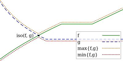
Figure 1: If $f$ increases and $g$ decreases, then for all $x:\min\{f(x),g(x)\}\leq\operatorname*{iso}(f,g)\leq\max\{f(x),g(x)\}$.

Next, we consider a sequential form of the isopoint operator and of the isopoint lemma, for the special case where $f(x)=x$ for $x\geq 0$.

Definition 5 (Isotuning sequence).

A pair $(X,g)$ is an isotuning sequence if the following conditions hold for all $t\in{\mathbb{N}}_{1}$: (i) $g_{t}:(g^{\text{low}}_{t},\infty)\to[0,\infty)$ is continuous and non-increasing, and define $g_{t}(g^{\text{low}}_{t})=\lim_{\varepsilon\to 0^{+}}g_{t}(g^{\text{low}}_{t}+\varepsilon)$, (ii) $g^{\text{low}}_{t}\leq X_{t-1}+g_{t}(g^{\text{low}}_{t})$, (iii) $X_{0}=0$, (iv) $X_{t}=\operatorname*{iso}_{y\geq g^{\text{low}}_{t}}(y,\ X_{t-1}+g_{t}(y))$, that is, $X_{t}\ =\ X_{t-1}+g_{t}(X_{t})$.

The associated domain bound sequence $g^{\inf}$ is defined as $g^{\inf}_{T}=\left(\max_{t\in[T]}g^{\text{low}}_{t}\right)_{\!+}$ for all $T\in{\mathbb{N}}_{1}$, and we set $g^{\inf}_{0}=0$. ∎

Condition (ii) ensures that $X_{t}$ exists and is unique, as proven in Appendix A.

Remark 6.

$\forall T\in{\mathbb{N}}_{1},X_{T}+\sum_{t=1}^{T}g_{t}(X_{t})\ =\ 2X_{T}$. ∎

We now give our central theorem, which bounds the isotuning sequence within a factor 2 of the optimal tuning in hindsight.

Theorem 7 (Isotuning).

Let $(X,g)$ be an isotuning sequence and define, for all $T\in{\mathbb{N}}_{0}$,

$$M_{T}(x)=x+\sum_{t\in[T]}g_{t}(x)\,,\quad\text{and}\quad M^{*}_{T}=\inf_{x>g^{\inf}_{T}}M_{T}(x)\,,$$

then for all $T\in{\mathbb{N}}_{0}$,

$$\tfrac{1}{2}M^{*}_{T}\leq\tfrac{1}{2}M_{T}(X_{T})\leq X_{T}=\sum_{t\in[T]}g_{t}(X_{t})\leq M^{*}_{T}\,.\qed$$

Proof.

For the lower bound, for all $t\in[T]$, since $g_{t}$ is non-increasing, and since $g^{\inf}_{T}\leq X_{T}$ we have

$$2X_{T} =X_{T}+\sum_{t\in[T]}g_{t}(X_{t})\geq X_{T}+\sum_{t\in[T]}g_{t}(X_{T})$$

$$=M_{T}(X_{T})\geq M^{*}_{T}\,.$$

For the upper bound, let $x^{*}_{T}=\operatorname*{arginf}_{x>g^{\inf}_{T}}M_{T}(x)$ and let $\tau=\min\{t\in[T]:X_{t}\geq x^{*}_{T}\}$. If $\tau$ does not exist then $X_{T}<x^{*}_{T}\leq M^{*}_{T}$, proving the claim. Otherwise, since $g_{t}$ is non-increasing then for all $t\geq\tau,g_{t}(X_{t})\leq g_{t}(x^{*}_{T})$ and so

$$X_{T} =X_{\tau-1}+\sum_{t=\tau}^{T}g_{t}(X_{t})\leq x^{*}_{T}+\sum_{t=\tau}^{T}g_{t}(x^{*}_{T})$$

$$\leq M_{T}(x^{*}_{T})=M^{*}_{T}\,.\qed$$

Example 8.

Consider the regret bound Eq. 1 of the introduction. Recall from Assumption 1 that $\Delta_{T}=q/\eta_{T}=\sum_{t}\delta_{t}$. Simply define $\delta_{t}=\eta_{t}a_{t}$, then:

$$\mathcal{R}_{T}(\bm{x}^{*})\leq\Delta_{T}+\sum_{t\in[T]}\delta_{t}=2\Delta_{T}\,.$$

Define $g_{t}(x)=qa_{t}/x$ such that $\delta_{t}=g_{t}(\Delta_{t})$ for all $t\in[T]$, then by Definition 5, $(\Delta,g)$ is an isotuning sequence (we can extend trivially $g_{t}(\cdot)=0$ for $t>T$), with $g^{\text{low}}_{t}=0$ and thus $g^{\inf}_{T}=\left(\max_{t}g^{\text{low}}_{t}\right)_{\!+}=0$. Hence, by 7 where $X_{t}\leadsto\Delta_{t}$ we obtain

$$\Delta_{T}\leq M^{*}_{T}=\inf_{y>0}\left\{y+\sum_{t\in[T]}\frac{qa_{t}}{y}\right\}=2\sqrt{q\sum_{t\in[T]}a_{t}}\,.\qed$$

Example 9.

To demonstrate the adaptivity of isotuning, assume instead that the regret bound is

$$\mathcal{R}_{T}(\bm{x}^{*})\leq\frac{q}{\eta_{T}}+\sum_{t\in[T]}\sqrt{\eta_{t}}a_{t}\,.$$

For example, such a bound can be extracted from Eq. 10 and Prop. 7 by Lattimore and Szepesvári (2020), in the context of partial monitoring. Then we also just set $\delta_{t}=\sqrt{\eta_{t}}a_{t}=\sqrt{q/\Delta_{t}}a_{t}$ and use Assumption 1, so by 7,

$$\mathcal{R}_{T} (\bm{x}^{*})\ \leq\ 2\Delta_{T}\ \leq\ 2M^{*}_{T}$$

$$=2\inf_{y>0}\left\{y+\sum_{t\in[T]}\sqrt{\frac{q}{y}}a_{t}\right\}=2cq^{\tfrac{1}{3}}\bigg{(}\sum_{t\in[T]}a_{t}\bigg{)}^{\tfrac{2}{3}}$$

where $c=2^{-\frac{2}{3}}+2^{\frac{1}{3}}$. Observe that with a change of variables we also have

$$\mathcal{R}_{T} (\bm{x}^{*})\leq 2\inf_{\eta>0}\left\{\frac{q}{\eta}+\sum_{t\in[T]}\sqrt{\eta}a_{t}\right\}$$

which again shows that the regret is within a factor 2 of the optimal learning rate in hindsight (for the same sequence of observations). ∎

3.2 Example: AOGD Revisited

Bartlett et al. (2007) propose an adaptive online gradient descent algorithm that automatically and sequentially adapts to the strong convexity of the loss functions, by using a balancing idea similar to that of isotuning to design a specific additional regularizer. For comparison, we recall their bound in Section A.2. We show how isotuning can recover their adaptive result while leading to simplified analysis, bound and algorithm, hence just by tuning the learning rate of online gradient descent and without an additional regularizer.

Assume that for all $t\in[T],\ell_{t}$ is $\alpha_{t}$-strongly convex, that is, for all $(x,y)\in\mathcal{X}^{2}$, $\ell_{t}(y)\geq\ell_{t}(x)+\langle y-x,\nabla\ell_{t}(x)\rangle+\frac{\alpha_{t}}{2}\|y-x\|_{2}^{2}$, We write $\nabla_{t}\equiv\nabla\ell_{t}(\bm{x}_{t})$. Define $\alpha_{1:t}=\sum_{s\in[t]}\alpha_{t}$, and $r_{t}=\ell_{t}(\bm{x}_{t})-\ell_{t}(\bm{x}^{*})$. We use the standard online gradient descent update with projection onto $\mathcal{X}$: $\bm{x}_{t+1}=\operatorname*{\Pi}_{\mathcal{X}}\left[\bm{x}_{t}-\eta_{t}\nabla_{t}\right]$.

By Lemma 31 (see Section A.2), we have, assuming $1/\eta_{0}=0$ and $\max_{t}\|\bm{x}_{t}-\bm{x}^{*}\|_{2}^{2}\leq D^{2}$ and taking $q=D^{2}$,

$$2\mathcal{R}_{T}(\bm{x}^{*})\leq\underbrace{q\left(\frac{1}{\eta_{T}}-\alpha_{1:T}\right)}_{(A)}+\underbrace{\sum_{t\in[T]}\eta_{t}\|\nabla_{t}\|^{2}}_{(B)}\,.$$

The term $(A)$ is decreasing with the learning rate, while the term $(B)$ is increasing with it. Hence, to balance the two terms, we define $\delta_{t}=\eta_{t}\|\nabla_{t}\|_{2}^{2}$ and $\Delta_{T}=\sum_{t\in[T]}\delta_{t}$, and we also define $\eta_{T}$ such that $\Delta_{T}=q(\frac{1}{\eta_{T}}-\alpha_{1:T})$. Thus,

$$\mathcal{R}_{T}(\bm{x}^{*})\leq\Delta_{T}\,.$$

Stepwise, this corresponds to the update

$$\Delta_{t} =\Delta_{t-1}+\delta_{t}$$

$$q\left(\frac{1}{\eta_{t}}-\alpha_{1:t}\right) =q\left(\frac{1}{\eta_{t-1}}-\alpha_{1:t-1}\right)+\eta_{t}\|\nabla_{t}\|_{2}^{2}$$

which is solved for $\eta^{-1}_{t}=\psi(\eta^{-1}_{t-1}+\alpha_{t},4\|\nabla_{t}\|_{2}^{2}/q)$ with $\psi(a,b)=(a+\sqrt{a^{2}+b})/2$; the learning rate $\eta_{t}$ is thus nonnegative non-increasing with $t$. To use 7, we need to express $\delta_{t}$ as a function of $\Delta_{t}$:

$$\delta_{t}=\eta_{t}\|\nabla_{t}\|_{2}^{2}=\frac{q\|\nabla_{t}\|_{2}^{2}}{\Delta_{t}+q\alpha_{1:t}}=:g_{t}(\Delta_{t})$$

and now applying 7 on the isotuning sequence $(\Delta,g)$ we obtain

$$\mathcal{R}_{T}(\bm{x}^{*}) \leq\inf_{y>0}\left\{y+\sum_{t\in[T]}\frac{q\|\nabla_{t}\|_{2}^{2}}{y+q\alpha_{1:t}}\right\}\,,$$

Finally, making a change of variables $z=y/q$ and recalling that $q=D^{2}$,

$$\mathcal{R}_{T}(\bm{x}^{*}) \leq\inf_{z>0}\left\{zD^{2}+\sum_{t\in[T]}\frac{\|\nabla_{t}\|_{2}^{2}}{z+\alpha_{1:t}}\right\}\,.$$

We have thus recovered (and slightly improved) the adaptivity to sequential strong-convexity of the original work (although in a simpler form): if $\alpha_{1:t}=\Omega(t)$ we can take $y=0$ and get a regret bound in $O(G^{2}\log T)$ where $G=\max_{t\in[T]}\|\nabla_{t}\|_{2}$, but even if $\alpha_{1:T}=0$ we also can take $y=D\sqrt{\sum_{t\in[T]}\|\nabla_{t}\|_{2}^{2}}$ to obtain a regret bounded by $2y$. All intermediate regimes can be retrieved as well.

3.3 A refined bound

7 is fairly general and can accommodate many cases, in particular since formulas of the form $X\leq\inf_{y}F(y)$ can easily be simplified by changes of variables, or by picking some good enough value for $y$. However, the special case $g_{t}(x)=\frac{a_{t}}{x}$ is frequent enough that is deserves a slightly improved bound.

Lemma 10.

Let $(X,g)$ be an isotuning sequence where $g_{t}(x)=a_{t}/x$ with $a_{t}\geq 0$ for all $t\in[T]$ then

$$X_{T}\leq\sqrt{2\sum_{t\in[T]}a_{t}}\,.$$

The result follows by Lemma 29 in Section A.1, and it can be easily adapted to various other cases where $g_{t}(x)\equiv a_{t}g(x)$ for $t\geq T_{1}$ for some $T_{1}$. When applicable, this improved bound saves a factor $\sqrt{2}$ over 7.

3.4 Online Correction

The standard analysis for online gradient descent (e.g., Hazan (2016)) leads a factor $\max_{t\in[T]}\|\bm{x}_{t}-\bm{x}^{*}\|^{2}\leq D^{2}$ in the regret bound. However, $D=\infty$ for unbounded domains. Some algorithms, such as FTRL, manage to have regret bounds that are centered on a fixed point (such as $\bm{x}_{1}$ or 0) and feature a term $\|\bm{x}_{1}-\bm{x}^{*}\|^{2}$ or $\|\bm{x}^{*}\|^{2}$ instead. (Even for bounded convex domains this is an improvement, see Example 42 in Appendix C). With constant learning rates, Mirror Descent is mostly equivalent to FTRL, but when using adaptive learning rates Mirror Descent usually does not provide centered bounds, and features a leading factor of $\max_{\bm{x}_{1},\bm{x}_{2}\in\mathcal{X}}B_{R}(\bm{x}_{1},\bm{x}_{2})$ instead. For bounded domains where the Bregman divergence is also bounded, this may be good enough and scale-free guarantees can be obtained (Orabona and Pál, 2018), but this factor can be infinite otherwise.

In this section we use the correction rule of Orseau et al. (2017) (see also Gyorgy and Szepesvari (2016); Fang et al. (2020)) to derive general centered regret bounds for a large class of algorithms beyond FTRL. While this correction rule was used for only one algorithm, we show that its usage can be extended to a much larger class, by contrast to other correction rules, such as the exponential correction of Györfi and Ottucsák (2007); Gaillard et al. (2014) (see also Chen et al. (2021); Huang et al. (2021) for other specific corrections). We use Assumption 1.

When deriving centered bounds, an additional difficulty appears: the learning rate becomes ‘off-by-one’ (McMahan, 2017, see also Lemma 12 below), that is, at step $t$ only the previous learning rate $\eta_{t-1}$ may be used, which means that the update cannot take into account, and adapt to the feedback received at step $t$.

At each step, we assume that the point $\bm{x}_{t}$ is first updated to $\bm{x}_{t^{\prime}}$ (in a problem-dependent way) using the previous learning rate $\eta_{t-1}$. Intuitively,

$${\displaystyle\bm{x}_{t^{\prime}}=\texttt{ \leavevmode\lstinline{{\lst@@@set@language\lst@@@set@numbers\lst@@@set@frame\lst@@@set@rulecolor\lst@@@set@frame\lst@@@set@language\lst@@@set@frame\color[rgb]{0,0,0}{\@listingGroup{ltx_lst_identifier}{update}}}}}}_{t}(\bm{x}_{t},\eta_{t-1})\,.$$ (2)

for some algorithm-specific update function. Then the following online correction (equivalent to that of  Orseau et al. (2017)) is applied:

$$\bm{x}_{t+1}=\bm{x}_{t^{\prime}}\frac{\Delta_{t-1}}{\Delta_{t}}+\frac{\delta_{t}}{\Delta_{t}}\bm{x}_{1}\,.$$ (3)

Lemma 11 (Online correction).

Let $f:\mathcal{X}\to{\mathbb{R}}$ be a convex function. Then, under Assumption 1, for all $t\in[T]$:

$$\Delta_{t}f(\bm{x}_{t+1})\leq\Delta_{t-1}f(\bm{x}_{t^{\prime}})+\delta_{t}f(\bm{x}_{1})\,,$$

and holds with equality if $f$ is affine. ∎

Proof.

Follows from $\Delta_{t-1}+\delta_{t}=\Delta_{t}$ and the convexity of $f$, then multiplying by $\Delta_{t}$ on both sides. ∎

Also observe that necessarily $\bm{x}_{t+1}\in\mathcal{X}$ if $\bm{x}_{t^{\prime}}\in\mathcal{X}$ and $\bm{x}_{1}\in\mathcal{X}$.

Recall that $\phi:\mathcal{X}\to{\mathbb{R}}$ is a convex function used to analyze the regret of the algorithm, and that $r_{t}$ is the instantaneous regret. Define for all $t\in{\mathbb{N}}_{1}$,

$$\delta^{*}_{t} =\left(\frac{1}{\eta_{t-1}}(\phi(\bm{x}_{t^{\prime}})-\phi(\bm{x}_{t}))+r_{t}\right)_{\!+}\,,$$ (4)

then we require

$$\delta_{t}\geq\delta^{*}_{t}\,.$$ (5)

In general, this inequality should be as tight as possible. See Algorithm 1. With these conditions we can provide a generic regret bound in this ‘off-by-one’ setting.

⬇

def generic_OCO_off_by_1($\bm{x}_{1}\!\in\!\mathcal{X},q\!>\!0$):

$\Delta_{0}=0$

for t = 1, 2, ...:

predict $\bm{x}_{t}$; observe $\ell_{t}$

$\eta_{t-1}=q/\Delta_{t-1}$ # off-by-one learning rate

$\bm{x}_{t^{\prime}}$ = update_t($\bm{x}_{t},\eta_{t-1}$) # off-by-one update

set $\delta_{t}$ s.t. $\delta_{t}\geq\left(\frac{1}{\eta_{t-1}}(\phi(\bm{x}_{t^{\prime}})-\phi(\bm{x}_{t}))+r_{t}\right)_{\!+}$ # found by analysis

$\Delta_{t}=\Delta_{t-1}+\delta_{t}$ # isotuning

$\bm{x}_{t+1}=\frac{\Delta_{t-1}}{\Delta_{t}}\bm{x}_{t^{\prime}}+\frac{\delta_{t}}{\Delta_{t}}\bm{x}_{1}$ # online correction

Algorithm 1 Generic online convex optimization algorithm sketch in the off-by-one setting. The update of $\eta_{t}$ usually has a closed form since $\delta_{t}$ depends on $\eta_{t-1}$ only.

Lemma 12 (Generic regret bound, off-by-one setting).

Consider Assumption 1. Let $\phi:\mathcal{X}\to{\mathbb{R}}$ be a convex function, and assume that $\delta_{t}$ satisfies Eq. 5. The regret of Algorithm 1 is bounded by

$$\mathcal{R}_{T}(\bm{x}^{*}) \leq\left(1+\frac{\phi_{1}}{q}-\frac{\phi_{T+1}}{q}\right)\Delta_{T}\,.\qed$$

Proof.

From Lemma 11 we have, since $\phi$ is convex,

$$\Delta_{t}\frac{\phi_{t+1}}{q} \leq\Delta_{t-1}\frac{\phi_{t}}{q}+\delta_{t}\frac{\phi_{1}}{q}+\Delta_{t-1}\left(\frac{\phi_{t^{\prime}}}{q}-\frac{\phi_{t}}{q}\right)$$

$$\Leftrightarrow\quad r_{t} \leq\Delta_{t-1}\frac{\phi_{t}}{q}-\Delta_{t}\frac{\phi_{t+1}}{q}+\delta_{t}\frac{\phi_{1}}{q}$$

$$\quad+\underbrace{\Delta_{t-1}\frac{\phi_{t^{\prime}}-\phi_{t}}{q}+r_{t}}_{\leq\delta_{t}}$$

$$\leq\Delta_{t-1}\frac{\phi_{t}}{q}-\Delta_{t}\frac{\phi_{t+1}}{q}+\left(1+\frac{\phi_{1}}{q}\right)\delta_{t}\,.$$

Summing over $t$ and telescoping gives:

$$\sum_{t\in[T]}r_{t} \leq\Delta_{0}\frac{\phi_{1}}{q}-\Delta_{T}\frac{\phi_{T+1}}{q}+\left(1+\frac{\phi_{1}}{q}\right)\sum_{t\in[T]}\delta_{t}$$

and the result follows from Assumption 1. ∎

Since, in the off-by-one setting, $\delta_{t}$ is a function of $\eta_{t-1}$ and thus of $\delta_{t-1}$ rather than $\Delta_{t}$, we provide a simple result to deal with this offset.

Lemma 13 (Isotuning offset).

Consider Assumption 1. For all $t\in{\mathbb{N}}_{1}$, let $\hat{\delta}_{t}:(0,\infty)\to[0,\infty)$ be continuous nonnegative non-increasing functions such that $\delta_{t}\leq\hat{\delta}_{t}(\Delta_{t}-b_{t})$ with $b_{t}\geq 0$. Assume $(\hat{\Delta},\hat{\delta})$ is an isotuning sequence. Then, for all $T\in{\mathbb{N}}_{1}$,

$$\Delta_{T}\ \leq\ \hat{\Delta}_{T}+\max_{t\in[T]}b_{t}\,.\qed$$

Proof.

Assume that $\Delta_{t-1}\leq\hat{\Delta}_{t-1}+\max_{s<t}b_{t}$, which is satisfied for $t=1$. Then

$${}\Delta_{t} \overset{\text{(a)}{}}{=}\min\{\Delta_{t},\ \Delta_{t-1}+\hat{\delta}(\Delta_{t}-b_{t})\}$$

$$\overset{\text{(b)}{}}{\leq}\operatorname*{iso}_{x\geq\left(\hat{\delta}^{\text{low}}_{t}+b_{t}\right)_{\!+}}\big{(}x,\ \Delta_{t-1}+\hat{\delta}(x-b_{t})\big{)}$$

$$\overset{\text{(c)}{}}{\leq}\max\{\hat{\Delta}_{t}+b_{t},\ \hat{\Delta}_{t-1}+\hat{\delta}_{t}(\hat{\Delta}_{t})+\max_{s<t}b_{s}\}$$

$$=\hat{\Delta}_{t}+\max_{s\leq t}b_{s}\,,$$

where (a) by assumption, (b) is by Lemma 3, (c) is also by Lemma 3 and taking $x=\hat{\Delta}_{t}+b_{t}$, and the result holds by induction. ∎

Remark 14.

Such offsets can also be dealt with directly with 7 by changes of variable. ∎

Corollary 15 (Off-by-one).

Consider the conditions of Lemma 13, and furthermore $\delta_{t}\leq\hat{\delta}_{t}(\Delta_{t-1})$. Then

$$\Delta_{T}\leq\hat{\Delta}_{T}+\max_{t\in[T]}\{\delta_{t}\}\,.\qed$$

Proof.

Follows from Lemma 13 where $b_{t}=\delta_{t}$. ∎

Note that Corollary 15 does not require that $\delta_{t}$ satisfies Eq. 5.

For bounded domains, even with unknown diameter, we can already easily obtain scale-free adaptive regret bounds. For example, consider online gradient descent using Algorithm 1 with the (off-by-one) update rule $\bm{x}_{t^{\prime}}=\bm{x}_{t}-\eta_{t-1}\nabla_{t}$. Following Eq. 5 with $\phi(\bm{x})=\|\bm{x}-\bm{x}^{*}\|^{2}/2$ (for some unknown $\bm{x}^{*}\in\mathcal{X}$) we can take $\delta_{t}=\eta_{t-1}\|\nabla_{t}\|^{2}/2=q\|\nabla_{t}\|^{2}/(2\Delta_{t-1})$. Define $\hat{\delta}_{t}(z)=q\|\nabla_{t}\|^{2}/(2z)$ such that $\delta_{t}\leq\hat{\delta}_{t}(\Delta_{t-1})$ for all $t\in[T]$, then from Lemmas 12, 15 and 7 we obtain

$$\mathcal{R}_{T}(\bm{x}^{*})\leq\left(1+\frac{\phi_{1}}{q}\right)\left(\sqrt{q\sum_{t\in[T]}\|\nabla_{t}\|^{2}}+\max_{t\in[T]}\delta_{t}\right)$$

From the update rule, we also have $\delta_{t}=\|\bm{x}_{t^{\prime}}-\bm{x}_{t}\|\|\nabla_{t}\|/2$, so for bounded domains $\delta_{t}\leq D\max_{t}\|\nabla_{t}\|/2$ even if $D$ is unknown. Using $\phi_{1}=\|\bm{x}_{1}-\bm{x}^{*}\|^{2}/2$ we thus have

$$\mathcal{R}_{T}(\bm{x}^{*})\leq\\ \left(1+\frac{\|\bm{x}^{*}-\bm{x}_{1}\|^{2}}{2q}\right)\left(\sqrt{q\sum_{t}\|\ell_{t}\|^{2}}+\frac{D}{2}\max_{t}\|\ell_{t}\|\right)$$

which fulfills our requirements of being centered, scale-free and adaptive to small losses. More discussion is given in Example 42. With unknown $D$, interesting choices for $q$ are $q=1$, but also $q=\|\mathbf{1}\|^{2}$, $q=\ln T$ or $q=\|\mathbf{1}\|^{2}\ln T$.

3.5 Null Updates

The additive term $\max_{t}\delta_{t}$ of Corollary 15 is unfortunately not well bounded if $D$ is overly large or infinite (e.g., , for partially constrained domains). For example, with $\mathcal{X}={\mathbb{R}}^{N}$, both $\|\bm{x}_{t^{\prime}}-\bm{x}_{t}\|$ and $\eta_{t-1}\|\nabla_{t}\|^{2}/2$ may be arbitrarily large, because $\eta_{t-1}$ may be too large compared to $\|\nabla_{t}\|_{2}$. And enforcing $\eta_{t-1}\leq 1$ would not lead to scale-free bounds, neither for small loss scales, nor for large loss scales. Note that small loss scales can matter for example when performing gradient descent on an almost flat surface.

At this point, we could use the loss clipping trick of Cutkosky (2019); Mhammedi et al. (2019) with off-by-one isotuning to obtain a bound very similar to the SOLO FTRL bound (hence with the additive $O(L\sqrt{T})$ term in unbounded domains). Instead, we consider another simple trick that will have additional benefits: updates that are too large, leading to large instantaneous regret, are simply skipped, similarly to skipping updates when delays are too large for bandit algorithms (Thune et al., 2019; Zimmert and Seldin, 2020). This corresponds to performing an update with a zero loss: $\bm{x}_{t^{\prime}}=\bm{x}_{t}$, which we call a null update, and, by contrast to using the doubling trick (Cesa-Bianchi et al., 1997) (see also Mhammedi et al. (2019)), the algorithm does not need to be additionally restarted. The instantaneous regret on null updates are dealt with separately (outside of $\Delta_{T}$), as demonstrated in the following generic result. We call $\mathcal{T}_{\emptyset}$ the set of steps where null updates are performed.

Theorem 16 (Generic regret bound, null updates).

Consider the assumptions of Lemma 12, but modify Algorithm 1 as follows: When $t\in\mathcal{T}_{\emptyset}$ set $\bm{x}_{t^{\prime}}=\bm{x}_{t}$, and set $\delta_{t}\geq 0$. Then the regret of the algorithm is at most

$$\mathcal{R}_{T}(\bm{x}^{*})\leq\left(1+\frac{\phi_{1}}{q}-\frac{\phi_{T+1}}{q}\right)\Delta_{T}+\sum_{t\in\mathcal{T}_{\emptyset}}(r_{t}-\delta_{t})\,.\qed$$

Proof.

Similar to the proof of Lemma 12, except that for $t\in\mathcal{T}_{\emptyset}$, $\phi_{t^{\prime}}=\phi_{t}$. ∎

Note that when $t\in\mathcal{T}_{\emptyset}$, it is important to set $\delta_{t}>0$ to increase $\Delta_{t}$ (and thus decrease $\eta_{t}$) and avoid triggering repeated null updates.

Consider the function $\hat{\delta}_{t}(\cdot)$ used in Corollary 15. We perform a null update at step $t$ when the instantaneous regret term coming from the update is larger than all previous ones added up, that is, when $\hat{\delta}_{t}(\Delta_{t-1})\geq c\Delta_{t-1}$ for some $c>0$. Define $\mathcal{T}_{\emptyset}=\{t\in[T]:\hat{\delta}_{t}(\Delta_{t-1})>c\Delta_{t-1}\}$ to be the set of steps where a null update is performed.

For $t\notin\mathcal{T}_{\emptyset}$, since $\delta_{t}\leq\hat{\delta}_{t}(\Delta_{t-1})\leq c\Delta_{t-1}$, using Lemma 3,

$$\delta_{t}\leq\hat{\delta}_{t}(\Delta_{t-1}) =\min\{\hat{\delta}_{t}(\Delta_{t-1}),\ c\Delta_{t-1}\}$$

$$\leq\operatorname*{iso}_{y>0}(\hat{\delta}_{t}(y),\ cy)\,.$$ (6)

This iso value has the particularity of being independent of $\Delta_{t-1}$ and thus of the learning rate $\eta_{t-1}$. For $\tau=\max\mathcal{T}_{\emptyset}$, the inequality is reversed, hence,

$$c\Delta_{\tau-1}\leq\operatorname*{iso}_{y>0}(\hat{\delta}_{\tau}(y),\ cy)\,.$$ (7)

Now, what value for $\delta_{t}$ should we choose when $t\in\mathcal{T}_{\emptyset}$ is a null update step? A good choice is again $\delta_{t}=\operatorname*{iso}_{y>0}(\hat{\delta}_{\tau}(y),\ cy)$, which ensures that for $t\in\mathcal{T}_{\emptyset}:c\Delta_{t-1}\leq\delta_{t}\leq\hat{\delta}_{t}(\Delta_{t-1})$. This ensures by Lemma 3 that for $t\notin\mathcal{T}_{\emptyset}:\delta_{t}\leq\hat{\delta}_{t}(\Delta_{t-1})\leq c\Delta_{t-1}$. We now provide a generic theorem that uses this particular value of $\delta_{t}$.

Theorem 17 (Isotuning with null updates).

Under the same conditions as Corollary 15, and additionally let $c>0$ and for $t\in\mathcal{T}_{\emptyset}$ set $\delta_{t}=\operatorname*{iso}_{y>0}(\hat{\delta}_{t}(y),\ cy)$. Then for all $T\in{\mathbb{N}}_{1}$ and with $\tau=\max\mathcal{T}_{\emptyset}$,

$$\Delta_{T} \leq\hat{\Delta}_{T}+\max_{t\in[T]}\{\operatorname*{iso}_{y>0}(\hat{\delta}_{t}(y),\ cy)\}\,,$$ (i)

$$\sum_{t\in\mathcal{T}_{\emptyset}}\delta_{t} \leq(\tfrac{1}{c}+1)\operatorname*{iso}_{y>0}(\hat{\delta}_{\tau}(y),\ cy)\,.$$ (ii)

Proof.

(i) For $t\in\mathcal{T}_{\emptyset},\delta_{t}=\operatorname*{iso}_{y>0}(\hat{\delta}_{t}(y),\ cy)\leq\max\{\hat{\delta}_{t}(\Delta_{t-1}),\ c\Delta_{t-1}\}=\hat{\delta}_{t}(\Delta_{t-1})$ by Lemma 3, hence for all $t\in[T]$, $\delta_{t}\leq\hat{\delta}_{t}(\Delta_{t-1})$, and we can then use Corollary 15. Moreover, for $t\notin\mathcal{T}_{\emptyset},\delta_{t}\leq\hat{\delta}_{t}(\Delta_{t-1})=\min\{\hat{\delta}_{t}(\Delta_{t-1}),\ c\Delta_{t-1}\}\leq\operatorname*{iso}_{y>0}(\hat{\delta}_{t}(y),\ cy)$, and thus $\max_{t}\delta_{t}\leq\max_{t}\operatorname*{iso}_{y>0}(\hat{\delta}_{t}(y),\ cy)$.

(ii) The result follows from $\sum_{t\in\mathcal{T}_{\emptyset}}\delta_{t}\leq\Delta_{\tau}=\Delta_{\tau-1}+\delta_{\tau}$ and Eqs. 6 and 7. ∎

Remark 18.

17 can be straightforwardly generalized from $cy$ to any sequence of continuous non-decreasing functions $\{f_{t}(y)\}_{t}$, including constant functions. ∎

Continuing our online gradient descent example, recall that $\hat{\delta}_{t}(y)=q\|\nabla_{t}\|^{2}/(2y)$, and thus $\operatorname*{iso}_{y>0}(q\|\nabla_{t}\|^{2}/(2y),y)=\sqrt{q/2}\|\nabla_{t}\|$. So if we perform null updates with $c=1$, that is, when $\eta_{t-1}\|\nabla_{t}\|^{2}/2>\Delta_{t-1}$ (or, equivalently, when $\sqrt{q/2}\|\nabla_{t}\|>\Delta_{t-1}$), then by 17 (and Lemma 10) we have

$$\Delta_{T}\leq\sqrt{q\sum_{t\in[T]}\|\nabla_{t}\|^{2}}+\sqrt{q/2}\max_{t}\|\nabla_{t}\|\,.$$

Thus, now the additive term is nicely bounded and does not depend on the diameter $D$. It remains to bound the regret incurred on null update rounds as per 16:

$$\sum_{t\in\mathcal{T}_{\emptyset}}r_{t} \leq\sum_{t\in\mathcal{T}_{\emptyset}}\|\bm{x}^{*}-\bm{x}_{t}\|\|\nabla_{t}\|$$

$$=\sum_{t\in\mathcal{T}_{\emptyset}}\|\bm{x}^{*}-\bm{x}_{t}\|\sqrt{2/q}\delta_{t}$$

$$\leq 2\max_{t\in\mathcal{T}_{\emptyset}}\|\bm{x}^{*}-\bm{x}_{t}\|\|\nabla_{\tau}\|$$

where we used 17 (ii) on the last line. Finally, $\max_{t\in\mathcal{T}_{\emptyset}}\|\bm{x}^{*}-\bm{x}_{t}\|$ is bounded by $D$, but also by $\|\bm{x}^{*}-\bm{x}_{1}\|+\sqrt{2q\tau}$ by Lemma 41 (in Appendix C), where $\tau=\max\mathcal{T}_{\emptyset}$.

Putting it all together we have

$$\mathcal{R}_{T}(\bm{x}^{*})\leq\\ \left(1+\frac{\|\bm{x}_{1}-\bm{x}^{*}\|^{2}}{2q}\right)\left(\sqrt{2q\sum_{t\in[T]}\|\nabla_{t}\|^{2}}+\sqrt{\frac{q}{2}}\max_{t}\|\nabla_{t}\|\right)\\ +2\min\{D,\ \|\bm{x}_{1}-\bm{x}^{*}\|+\sqrt{2q\tau}\}\|\nabla_{\tau}\|\,.$$

Now the main difference with the SOLO-FTRL bound (Orabona and Pál, 2018) is that we have the term $\sqrt{\tau}\|\nabla_{\tau}\|$ instead of $\sqrt{T}\max_{t\in[T]}\|\nabla_{t}\|$. Naturally, we wish to understand how much of an improvement this is. First of all, since $\tau\leq T$, our bound is never worse. Furthermore, since $\delta_{\tau}\geq\Delta_{\tau-1}\geq\sum_{t\in\mathcal{T}_{\emptyset}\setminus\{\tau\}}\delta_{t}$ we have $\|\nabla_{\tau}\|\geq\sum_{t\in\mathcal{T}_{\emptyset}\setminus\{\tau\}}\|\nabla_{t}\|$. This means that a null update is triggered only when the loss is larger than the cumulative losses on all previous null updates. We can draw a few observations: (i) unless losses grow exponentially forever (which makes learning rather difficult), $\tau$ has a finite value even as $T$ grows; (ii) if losses are i.i.d.​ from a bounded distribution, large losses are observed exponentially fast and thus $\tau$ is necessarily small; (iii) when performing gradient descent on a convex surface, the largest losses are usually observed during the first few steps and then $\tau=O(1)$.

The most likely ‘bad’ scenario is when very small gradients $\ell$ are observed for $T-1$ steps and on the $T$-th step a large loss $L$ is incurred (possibly $\bm{x}_{1}$ starts on a plateau and the loss function is only quasiconvex). Moreover, we will prove in Appendix B that $\|\nabla_{\tau}\|^{2}\geq\sum_{t<\tau}\|\nabla_{t}\|^{2}$. This means that in this scenario, to trigger a null update, we must have $L\geq\sqrt{T}\ell$, even if only one null update has been triggered before. Hence, as long as losses do not grow faster than a factor $\sqrt{T}$, no null update is triggered.

Hence, for most situations, the adaptivity to small quadratic losses $\sqrt{\sum_{t}\|\nabla_{t}\|^{2}}$ is restored.

4 APPLICATIONS

We apply our tools to several algorithms: scale-free FTRL, scale-free Mirror Descent, and scale-free Prod, scale-free Adapt-ML-Prod, and also a slight generalization of AdaHedge (Appendix E) and a refinement of Soft-Bayes (Appendix F). We now consider linear losses $\ell_{t}\in{\mathbb{R}}^{N}$. For the first two applications, the instantaneous regret is $r_{t}=\langle\bm{x}_{t}-\bm{x}^{*},\ell_{t}\rangle$.

4.1 Scale-Free FTRL

In this section we show how the results we obtain for online gradient descent in Section 3.5 can be generalized to FTRL with any regularizer that is 1-strongly convex to a given norm $\|\cdot\|$. As discussed in Section 3.5, we use null updates to restore the adaptivity to small losses for unbounded domains, that was lost for the SOLO FTRL regret bound whose regret is dominated by the $O(L\sqrt{T})$ term, where $L=\max_{t\in[T]}\|\ell_{t}\|_{*}$.

We first consider FTRL with isotuning but without null updates (similar to AdaFTRL (Orabona and Pál, 2018, appendix B.1)), then we construct a meta-algorithm that filters out the exceedingly large losses before sending the losses to the subalgorithm. The resulting (compound) algorithm is called isoFTRL (see Algorithm 2).

⬇

def isoFTRL($\mathcal{X},R,q>0$):

$L_{0}=0$; $\Delta_{0}=0$

for t = 1, 2, 3, ...:

$\eta=q/\Delta_{t-1}$ # ${\color[rgb]{.8,.4,0}\eta_{t-1}}$

$\bm{x}_{t}=\operatorname*{argmin}_{\bm{x}\in\mathcal{X}}\left\{\langle\tilde{L}_{t-1},\bm{x}\rangle+\frac{R(\bm{x})}{\eta}\right\}$

predict $\bm{x}_{t}$; observe $\ell_{t}$

if $\tfrac{1}{2}\eta\|\ell_{t}\|_{*}^{2}\leq\Delta_{t-1}$: # or ${\color[rgb]{.8,.4,0}\sqrt{q/2}\|\ell_{t}\|_{*}\leq\Delta_{t-1}}$

$\delta_{t}=\tfrac{1}{2}\eta\|\ell_{t}\|_{*}^{2}$ # from Eq. 5

$\tilde{\ell}_{t}=\ell_{t}$

else:

$\delta_{t}=\sqrt{\tfrac{1}{2}q}\|\ell_{t}\|_{*}$ # isopoint

$\tilde{\ell}_{t}=0$ # null update

$\tilde{L}_{t}=\tilde{L}_{t-1}+\tilde{\ell}_{t}$

$\Delta_{t}=\Delta_{t-1}+\delta_{t}$ # isotuning

Algorithm 2 FTRL with null updates and isotuning

First we recall (and slightly generalize) an intermediate bound for AdaFTRL.

Lemma 19 (AdaFTRL, Orabona and Pál (2018), Lemma 5).

Consider Assumption 1, and $\delta_{t}\geq B_{R^{*}}(-\eta_{t-1}L_{t},-\eta_{t-1}L_{t-1})/\eta_{t-1}$. Then the regret of FTRL with isotuning to any $\bm{x}^{*}\in\mathcal{X}$ is bounded by

$$\mathcal{R}_{T}(\bm{x}^{*})\leq\left(1+\frac{R(\bm{x}^{*})}{q}\right)\Delta_{T}\,.$$

We now describe isotuning FTRL with null updates, see Algorithm 2. Recall that the regularizer $R$ is 1-strongly convex with respect to the norm $\|\cdot\|$. Define $\hat{\delta}_{t}(y)=\frac{q}{2y}\|\ell_{t}\|_{*}^{2}$. From Section 3.5 we take $c=1$, and recall that $\mathcal{T}_{\emptyset}=\{t\in[T]:\hat{\delta}_{t}(\Delta_{t-1})>\Delta_{t-1}\}$ is the set of steps where a null update is performed, then we run FTRL with modified losses $\tilde{\ell}_{t}=\ell_{t}\left[\!\left[t\notin\mathcal{T}_{\emptyset}\right]\!\right]$. Furthermore, define

$$\delta_{t}=\begin{cases}\operatorname*{iso}_{y>0}\left(q\frac{\|\ell_{t}\|_{*}^{2}}{2y},\ y\right)=\sqrt{\tfrac{1}{2}q}\|\ell_{t}\|_{*}&\text{ when }t\in\mathcal{T}_{\emptyset}\,,\\ \hat{\delta}_{t}(\Delta_{t-1})&\text{ otherwise.}\end{cases}$$

Then $\delta_{t}\geq B_{R^{*}}(-\eta_{t-1}\tilde{L}_{t},-\eta_{t-1}\tilde{L}_{t-1})/\eta_{t-1}$ by proposition 2 of Orabona and Pál (2018).

Then we can show the following bound. The proof is in Appendix B.

Theorem 20.

The regret of isoFTRL (Algorithm 2) is bounded by

$$\mathcal{R}_{T}(\bm{x}^{*})\leq\\ \left(\sqrt{q}+\frac{R(\bm{x}^{*})}{\sqrt{q}}\right)\left(\sqrt{\sum_{t\in[T]}\|\ell_{t}\|_{*}^{2}}+\tfrac{1}{\sqrt{2}}\max_{t}\|\ell_{t}\|_{*}\right)\\ +2\min\left\{D,\ \sqrt{2R(\bm{x}^{*})}+2\sqrt{2q\tau}\right\}\|\ell_{\tau}\|_{*}\,,$$

where $\tau=\max\mathcal{T}_{\emptyset}$ is the last step a null update is performed, and is such that $\|\ell_{\tau}\|_{*}^{2}\ \geq\ \sum_{t<\tau}\|\ell_{t}\|_{*}^{2}$. ∎

4.2 Scale-Free Mirror Descent

Orabona and Pál (2018) provide two lower bounds showing that their scale-free Mirror Descent (meant for bounded maximum Bregman divergence between any two points) fails with (super)linear regret: the first one is for the quadratic regularizer (gradient descent), and the second one is for the entropic regularizer for which the Bregman divergence is the relative entropy, which is not bounded even though the regularizer is bounded.

We now propose a scale-free variant of the Mirror Descent algorithm with null updates, isotuning and online correction, for bounded and unbounded domains, at least for Bregman divergences that are convex in their second argument, including the quadratic and the entropic regularizers. The two lower bound examples mentioned above do not apply to our algorithm, thanks to using the online correction to center the bound, leading to a factor $B_{R}(\bm{x}^{*},\bm{x}_{1})$ instead of $\sup_{(\bm{x},\bm{x}^{\prime})\in\mathcal{X}^{2}}B_{R}(\bm{x},\bm{x}^{\prime})$. Choosing $\bm{x}_{1}=\operatorname*{argmin}_{\bm{x}\in\mathcal{X}}R(\bm{x})$ ensures that $\phi_{1}=B_{R}(\bm{x}^{*},\bm{x}_{1})\leq R(\bm{x}^{*})-R(\bm{x}_{1})$ similarly to FTRL, but in general one should take $\bm{x}_{1}=\operatorname*{argmin}_{\bm{x}\in\mathcal{X}}\max_{\bm{x}^{*}\in\mathcal{X}}B_{R}(\bm{x}^{*},\bm{x})$. In particular, when $R(\bm{x})=\tfrac{1}{2}\|\bm{x}\|_{2}^{2}$, then by Jung’s theorem we have $\|\bm{x}^{*}-\bm{x}_{1}\|_{2}\leq D/\sqrt{2}$ and thus we can take $q=(D/\sqrt{2})^{2}/2=D^{2}/4$. See additional discussion in Example 42.

The algorithm is described in Algorithm 3. For null updates, we take $c=1$ also.

⬇

def isoMD($\mathcal{X}$, $R$, $q>0$):

$\Delta_{0}=0$ ; $\bm{x}_{1}=\operatorname*{argmin}_{\bm{x}\in\mathcal{X}}\max_{\bm{x}^{\prime}\in\mathcal{X}}B_{R}(\bm{x}^{\prime},\bm{x})$

for t = 1, 2, ...:

predict $\bm{x}_{t}$; observe $\ell_{t}$

$\eta=q/\Delta_{t-1}$

if $\tfrac{1}{2}\eta\|\ell_{t}\|_{*}^{2}\leq\Delta_{t-1}$: # or ${\color[rgb]{.8,.4,0}\sqrt{q/2}\|\ell_{t}\|_{*}\leq\Delta_{t-1}}$

$\bm{x}_{t^{\prime}}=\operatorname*{argmin}_{\bm{x}\in\mathcal{X}}\left\{\langle\bm{x},\ell_{t}\rangle+\frac{B_{R}(\bm{x},\bm{x}_{t})}{\eta}\right\}$

$\delta_{t}=\tfrac{1}{2}\eta\|\ell_{t}\|_{*}^{2}$ # from Eq. 5

else:

$\bm{x}_{t^{\prime}}=\bm{x}_{t}$ # null update

$\delta_{t}=\sqrt{\tfrac{1}{2}q}\|\ell_{t}\|_{*}$ # isopoint

$\Delta_{t}=\Delta_{t-1}+\delta_{t}$ # isotuning

$\bm{x}_{t+1}=\frac{\Delta_{t-1}}{\Delta_{t}}\bm{x}_{t^{\prime}}+\frac{\delta_{t}}{\Delta_{t}}\bm{x}_{1}$ # online cor.

Algorithm 3 Scale-free Mirror Descent for bounded and unbounded decision sets.

In this section we take $\phi_{t}=B_{R}(\bm{x}^{*},\bm{x}_{t})$, and recall that $\phi(\cdot)$ must be convex.

Theorem 21.

With $\phi_{1}=B_{R}(\bm{x}^{*},\bm{x}_{1})$, the regret of isoMD (Algorithm 3) is bounded by

$$\mathcal{R}_{T}(\bm{x}^{*})\leq\\ \left(\sqrt{q}+\frac{\phi_{1}}{\sqrt{q}}\right)\left(\sqrt{\sum_{t\notin\mathcal{T}_{\emptyset}}\|\ell_{t}\|_{*}^{2}}+\tfrac{1}{\sqrt{2}}\max_{t\in[T]}\|\ell_{t}\|_{*}\right)\\ +2\min\{D,\ \|\bm{x}^{*}-\bm{x}_{1}\|+\sqrt{2q\tau}\}\|\ell_{\tau}\|_{*}\,,$$

where $\tau=\max\mathcal{T}_{\emptyset}$ is the last step a null update is performed, and is such that $\|\ell_{\tau}\|_{*}^{2}\ \geq\ \sum_{t<\tau}\|\ell_{t}\|_{*}^{2}$. ∎

The proof is given in Appendix C.

4.3 Scale-free adaptive Prod

The Prod family of algorithms (Cesa-Bianchi et al., 2007; Gaillard et al., 2014; Sani et al., 2014; Orseau et al., 2017) are based on Mirror-Descent style multiplicative updates, but their analysis does not fit either the MD nor the FTRL analysis framework. Previous works have resorted to more or less ad-hoc analysis. They can be analysed, however, with our generic off-by-one setting and online correction, and only the quantity of interest $\delta_{t}$ needs to be bounded as per Eq. 5 on an algorithm-dependent basis, taking $\phi(\bm{x})=\text{RE}(\bm{x}^{*}\|\bm{x})=\sum_{i\in[N]}\bm{x}^{*}_{i}\ln(\bm{x}^{*}_{i}/\bm{x}_{i})$. Also see Appendix F for a slightly simplified sparse Soft-Bayes algorithm (Orseau et al., 2017) and enhanced regret bound.

In this section, we demonstrate how to obtain a scale free and adaptive version of the Prod algorithm (Cesa-Bianchi et al., 2007; Gaillard et al., 2014) with a single learning rate. This algorithm was originally analyzed with constant learning rates and a doubling trick with restarts (Cesa-Bianchi et al., 2007). While this single learning-rate algorithm is not so useful in itself in practice as it can be advantageously replaced with AdaHedge (de Rooij et al., 2014), the example is technically useful as it shows how some constraints of the update rule can be easily tackled with null updates, while demonstrating how the tools we built in the previous sections lead to a straightforward analysis of the regret. It also serves as a prelude to the next section where we analyse the multiple learning rate version. It also uses Lemma 46 which tightens the leading constant factor by $\sqrt{2}$ on lower bounding $\log(1+x)$ compared to Lemma 1 of Cesa-Bianchi et al. (2007).

We use Assumption 1, and Algorithm 1 with null updates—but without a doubling trick or any restarting. The decision set $\mathcal{X}$ is the probability simplex of $N$ coordinates, and we take $\phi(\bm{x})=\text{RE}(\bm{x}^{*}\|\bm{x})$ and $q=\phi_{1}=\ln N$.

For all $t\in[T]$, let $\ell_{t}\in{\mathbb{R}}^{N}$, and define $\bar{\ell}_{t}=\sum_{i\in[N]}\bm{x}_{i,t}\ell_{i,t}$.

Define the prod update (off by one):

$$\bm{x}_{1} =\left(\frac{1}{N},\dots,\frac{1}{N}\right)$$

$$\forall i\in[N]:\bm{x}_{i,t^{\prime}} =\bm{x}_{i,t}(1+\eta_{i,t-1}(\bar{\ell}_{t}-\ell_{i,t}))$$ (8)

For all $t$, define $s_{t}=\max_{i}|\bar{\ell}_{t}-\ell_{i,t}|$ and $\hat{\delta}_{t}(x)=\frac{qs_{t}^{2}}{2x}$, with $\hat{\delta}_{t}(x)=\infty$ for $x\leq 0$.

As per Eq. 5, for $t\notin\mathcal{T}_{\emptyset}$, we can define

$$\delta_{t}=\max_{i}\left(\frac{-1}{\eta_{t-1}}\ln(1+\eta_{t-1}(\bar{\ell}_{t}-\ell_{i,t}))+(\bar{\ell}_{t}-\ell_{i,t})\right)\,,$$

and by Lemma 46, we have that, when $\Delta_{t-1}-qs_{t}>0$,

$$\delta_{t}\leq\hat{\delta}_{t}(\Delta_{t-1}-qs_{t})=\hat{\delta}_{t}(\Delta_{t}-\delta_{t}-qs_{t})\,.$$ (9)

The update in Eq. 8 may be invalid (non-positive) when $1-\eta_{t-1}s_{t}\leq 0$, which corresponds to $\Delta_{t-1}-qs_{t}\leq 0$, in which case $\hat{\delta}_{t}(\Delta_{t-1}-qs_{t})=\infty$. To avoid this we perform a null update when $\hat{\delta}_{t}(\Delta_{t-1}-qs_{t})>\Delta_{t-1}-qs_{t}$, in which case ($t\in\mathcal{T}_{\emptyset}$) we set $\delta_{t}=\operatorname*{iso}_{y>0}(\hat{\delta}_{t}(y),y)=\sqrt{\frac{q}{2}}s_{t}$, which ensures by Lemma 3 that

$$\forall t\notin\mathcal{T}_{\emptyset}: \delta_{t}\leq\hat{\delta}_{t}(\Delta_{t-1}-qs_{t})\leq\sqrt{\frac{q}{2}}s_{t}\leq\Delta_{t-1}-qs_{t}\,,$$

$$\forall t\in\mathcal{T}_{\emptyset}: \Delta_{t-1}-qs_{t}\leq\delta_{t}=\sqrt{\frac{q}{2}}s_{t}\leq\hat{\delta}_{t}(\Delta_{t-1}-qs_{t})\,.$$

We call isoProd the resulting algorithm.

Theorem 22.

Let $S=\max_{t\in[T]}s_{t}$. The regret of isoProd is bounded by

$$\mathcal{R}_{T}(\bm{x}^{*})\leq 2\sqrt{\ln(N)\sum_{t}s_{t}^{2}}+S(2\ln N+\sqrt{2\ln N}+2)\,.$$

Proof.

By 16 we have $\mathcal{R}_{T}(\bm{x}^{*})\leq 2\Delta_{T}+\sum_{t\in\mathcal{T}_{\emptyset}}(r_{t}-\delta_{t})$. Since $r_{t}\leq s_{t}=\sqrt{2/q}\delta_{t}$ for $t\in\mathcal{T}_{\emptyset}$,

$$\sum_{t\in\mathcal{T}_{\emptyset}}(r_{t}-\delta_{t}) \leq(\sqrt{2/q}-1)\sum_{t\in\mathcal{T}_{\emptyset}}\delta_{t}$$

$$\leq(\sqrt{2/q}-1)(\Delta_{\tau-1}+\delta_{\tau})$$

$$\leq(\sqrt{2/q}-1)(\sqrt{q/2}s_{\tau}+qs_{\tau}+\sqrt{q/2}s_{\tau})$$

$$\leq 2S\,,$$

where $\tau=\max\mathcal{T}_{\emptyset}$, and we used $\Delta_{t-1}-qs_{t}\leq\delta_{t}$ for $t\in\mathcal{T}_{\emptyset}$. Let $(\hat{\Delta},\hat{\delta})$ be an isotuning sequence, then by Lemma 13 and Eq. 9 we know that $\Delta_{T}\leq\hat{\Delta}_{T}+\max_{t}\{\delta_{t}+qs_{t}\}\leq\hat{\Delta}_{T}+\sqrt{q/2}S+qS$. Finally by Lemma 10 we have $\hat{\Delta}_{T}\leq\sqrt{q\sum_{t}s_{t}^{2}}$. ∎

Remark 23.

Alternatively, we could use the update

$$\bm{x}_{i,t^{\prime}} =\bm{x}_{i,t}\frac{1-\eta_{t-1}\ell_{i,t}}{1-\eta_{t-1}\bar{\ell}_{t}}$$

which leads to $\delta_{t}=\max_{i}\eta_{t-1}\frac{\ell_{i,t}^{2}/2}{1-\eta_{t-1}\ell_{i,t}}$ and thus $\mathcal{R}_{T}(\bm{x}^{*})=O(\sqrt{q\sum_{t}\max_{i}\ell_{i,t}^{2}})$ and then use Lemma 48 to sequentially translate the losses arbitrarily. ∎

4.4 Scale-free Adapt-ML-Prod

Gaillard et al. (2014) propose the Adapt-ML-Prod algorithm, for losses in $[0,1]$ with multiple learning rates, to obtain a regret bound which depends only on the excess losses $\sqrt{\sum_{t}(\bar{\ell}_{t}-\ell_{i,t})^{2}}$ to the best expert $i$ in hindsight, where $\bar{\ell}_{t}$ is the loss incurred by the algorithm and $\ell_{i,t}$ is the loss incurred by the expert $i$ at step $t$ and show interesting consequences of this bound, in particular it is bounded by a constant in expectation when losses are i.i.d. By contrast, AdaHedge (de Rooij et al., 2014; van Erven et al., 2011) can tackle losses with unknown range, but has a regret bound featuring the quantity $\sqrt{\sum_{t}\sum_{i\in[N]}\bm{x}_{i,t}(\bar{\ell}_{t}-\ell_{i,t})^{2}}$ instead. We extend Adapt-ML-Prod to tackle unbounded and unknown loss ranges using isotuning, online correction, and null updates—or equivalently we extend isoProd of the previous section to using one learning rate per expert.

Gaillard et al. consider losses in $[0,1]$, and their algorithm predicts with positive weights $\propto\bm{x}_{i,t}\eta_{i,t-1}$ and suffers the loss

$$\bar{\ell}_{t}=\sum_{i\in[N]}\frac{\bm{x}_{i,t}\eta_{i,t-1}}{\sum_{j\in[N]}\bm{x}_{j,t}\eta_{j,t-1}}\ell_{i,t}\,.$$ (10)

For all $T\in{\mathbb{N}}_{1},\forall i\in[N]$, define $r_{i,t}=\bar{\ell}_{t}-\ell_{i,t}$ and $\mathcal{R}_{i,T}=\sum_{t\in[T]}r_{i,t}$, also $V_{i,T}=\sum_{t\in[T]}r_{i,t}^{2}$, and $s_{t}=\max_{i\in[N]}|r_{i,t}|$. Assuming $N\geq 2$ and $T\geq 2$, we can rewrite the regret bound of Adapt-ML-Prod (Gaillard et al., 2014, Corollary 4) to the best expert $i$ in hindsight as:

$$\mathcal{R}_{i,T}\leq\left[\sqrt{\left(1+V_{i,T}\right)\ln N}+3\ln N\right]\!\left[4+\frac{1+\ln\ln T}{\ln N}\right].$$

Note, for $T=10^{40}$ and $N\geq 4$, $(1+\ln\ln T)/\ln N<4$.

Adapt-ML-Prod is meant for losses in $[0,1]$ and can be used for losses in any $[a,b]$ if an upper bound on $b-a$ is known. However, when the loss range is not known beforehand, as for isoProd we perform a null update when the update may lead to invalid (negative) weights. We obtain an algorithm with a regret guarantee that is just as good as when the loss range is known beforehand.

As for Adapt-ML-Prod, our algorithm uses one learning rate per coordinate, and the tools of the previous sections will apply almost always coordinate-wise. For all $i\in[N]$, we first define the update $\bm{x}_{i,t^{\prime}}$ for Adapt-ML-Prod:

$$\bm{x}_{i,1} =1\,,$$

$$\bm{x}_{i,t^{\prime}} =\bm{x}_{i,t}(1+\eta_{i,t-1}(\bar{\ell}_{t}-\ell_{i,t}))\,,$$ (11)

and then apply the online correction of Eq. 3. As for Prod, the problem with Eq. 11 is that it is invalid when $\bm{x}_{i,t^{\prime}}$ becomes negative. We prevent this issue by performing null updates ($t\in\mathcal{T}_{\emptyset}$) whenever $\eta_{i,t-1}|\bar{\ell}_{t}-\ell_{i,t}|\geq 1/2$ for some $i\in[N]$, that is, $q|\bar{\ell}_{t}-\ell_{i,t}|\geq\Delta_{i,t-1}/2$. Note that to ensure that $\sum_{i}\bm{x}_{i,t^{\prime}}=\sum_{i}\bm{x}_{i,t}$ for all rounds $t$ (as will be shown in the proof of 24), we perform a null update on all coordinates at the same time, which leads to an additional difficulty compared to isoProd, as $\hat{\delta}_{i,t}(\Delta_{i,t})>c\Delta_{i,t-1}$ is not always true when $t\in\mathcal{T}_{\emptyset}$.

We use Assumption 1 and we take $\phi_{i}(\bm{x}_{i,t})=-\ln\bm{x}_{i,t}$ for all $i\in[N]$, and $\mathcal{X}=[0,\infty)^{N}$. Set $q=\ln N$. and, recalling that $r_{i,t}=\bar{\ell}_{t}-\ell_{i,t}$ and $s_{t}=\max_{i}|r_{i,t}|$, define from Eq. 5

$$t\notin\mathcal{T}_{\emptyset}:\delta_{i,t} =\delta^{*}_{i,t}=r_{i,t}-\frac{1}{\eta_{i,t-1}}\ln(1+\eta_{i,t-1}r_{i,t})\,,$$

$$t\in\mathcal{T}_{\emptyset}:\delta_{i,t} =s_{t}\,.$$

On a null update we set $\delta_{i,t}=s_{t}$, so that $\delta_{i,t}\geq r_{i,t}$ conveniently absorbs the instantaneous regret; note that we do not set $\delta_{i,t}=|\bar{\ell}_{t}-\ell_{i,t}|$ to avoid triggering null updates of the same scale $N$ times, which would lead to an additive term $O(N\max_{t}|r_{i,t}|)$ in the bound instead of $O(\max_{j,t}|r_{j,t}|)$.

Observe that $\phi_{i,1}=0$, so from 16, since also $\delta_{i,t}\geq r_{i,t}$ for $t\in\mathcal{T}_{\emptyset}$, we can simplify:

$$\mathcal{R}_{i,T}\leq\left(1+\frac{\ln\bm{x}_{i,T+1}}{\ln N}\right)\Delta_{i,T}\,.$$ (12)

We call the resulting algorithm isoML-Prod (see Algorithm 4) and we prove an adaptive scale-free bound. The proof is given in Appendix D.

⬇

def isoML_Prod():

$\forall i\in[N]:\Delta_{i,0}=0,\bm{x}_{i,1}=1$

for t = 1, 2, ...:

$\forall i\in[N]:\tilde{\bm{x}}_{i,t}=\bm{x}_{i,t}/\Delta_{i,t-1}$

Predict normalized $\tilde{\bm{x}}$; observe $\ell_{t}$

$\bar{\ell}_{t}=\sum_{i\in[N]}\tilde{\bm{x}}_{i,t}\ell_{i,t}\,/\,\sum_{i\in[N]}\tilde{\bm{x}}_{i,t}$

for each $i\in[N]$:

if $\max_{j\in[N]}q|\bar{\ell}_{t}-\ell_{j,t}|<\Delta_{j,t-1}$:

$r=\bar{\ell}_{t}-\ell_{i,t}$

$\eta=\ln N/\Delta_{i,t-1}$

# Adapt-ML-Prod (core) update:

$\bm{x}^{\prime}_{i,t}=\bm{x}_{i,t}(1+\eta r)$

$\delta_{i,t}=r-\frac{1}{\eta}\ln(1+\eta r)$ # isotuning

else: # ${\color[rgb]{.8,.4,0}t\in\mathcal{T}_{\emptyset}}$

$\bm{x}^{\prime}_{i,t}=\bm{x}_{i,t}$ # null update

$\delta_{i,t}=\max_{j\in[N]}|\bar{\ell}_{t}-\ell_{j,t}|$

$\Delta_{i,t}=\Delta_{i,t-1}+\delta_{i,t}$ # isotuning

$\bm{x}_{i,t+1}=\bm{x}^{\prime}_{i,t}\frac{\Delta_{i,t-1}}{\Delta_{i,t}}+\frac{\delta_{i,t}}{\Delta_{i,t}}\bm{x}_{i,1}$ # online cor.

Algorithm 4 The isoML-Prod algorithm, which uses one learning rate per coordinate and does not have prior knowledge of the range of the losses.

Theorem 24.

Assume $N\geq 2$. We consider losses $\ell_{i,t}\in{\mathbb{R}}$ for all experts $i\in[N]$ and time steps $t\in{\mathbb{N}}_{1}$. Let $S=\max_{t\in[T]}s_{t}$. Then for all $i\in[N]$, of isoML-Prod is bounded by

$$\mathcal{R}_{i,T}\leq\left[\sqrt{V_{i,T}\ln N}+S(2+3\ln N)\right]\left[2+\frac{\ln(1+C)}{\ln N}\right]$$

where simultaneously $C\leq T$, $C\leq\tau+\ln\frac{ST}{s_{\tau}}$, and also $C=o(1)+\ln ST$. ∎

5 RELATED WORK

Null updates.

Skipping updates was used in the bandit literature to avoid a large penalty due to long delays (Thune et al., 2019; Zimmert and Seldin, 2020). Concurrently to this paper, Huang et al. (2021) extend this line of work to obtain scale-free (but only partially adaptive) guarantees in the same context.

Online correction.

Our use of the online correction comes from Orseau et al. (2017), which is based on the Fixed Share rule (Herbster and Warmuth, 1998a). We have been informed after a first version of this paper that it is to the primal stabilization technique of Fang et al. (2020), who also propose a more general stabilization technique in the dual space which does not require the Bregman divergence to be convex in its second argument. Other correction terms appear in the literature for more specific purposes, e.g., Gaillard et al. (2014); Chen et al. (2021); Huang et al. (2021).

Loss clipping.

To tackle the off-by-one issue, Cutkosky (2019) proposes a correction term of the loss scales, at the expense of an additive term $\max_{t}\|\bm{x}_{t}-\bm{x}^{*}\|\max_{t}\|\ell_{t}\|$, and requires a special treatment for $t=0$ akin to a null update. In itself, this correction is not enough and must be combined with an additional mechanism such as the restarting of Mhammedi et al. (2019) to obtain scale-free regret bounds. The SOLO-FTRL bound can easily be recovered with this combination, but not apparently that of 20 and, by contrast to null updates, it does not help dealing with constraint violations of the update rule as for Prod (Section 4.3), or the offsets in the Prod (Section 4.3) and AdaHedge (Appendix E) bounds. Null updates, combined with isotuning and in particular Corollary 15, avoid the need to restart the algorithm altogether.

Isotuning.

As mentioned before, the isotuning assumptions of Assumption 1 come from the AdaHedge update scheme (de Rooij et al., 2014), and were adapted to FTRL in AdaFTRL only for domains with bounded diameter and bounded Bregman divergence (Orabona and Pál, 2018). A form of isotuning also appears in Bartlett et al. (2007) (see Section 3.2). These works use a more ad-hoc analysis of the $\Delta_{T}$ quantity, while we provide a general framework where we only need to express $\delta_{t}$ as a function of $\Delta_{t}$ and then invoke 7 to obtain a first bound. The off-by-one issue is trivially dealt with in AdaHedge because the additive term $\max_{t}\delta_{t}$ is bounded by the maximum loss range (see Appendix E), and is only partially dealt with in AdaFTRL, leading to the heavy constraints mentioned above. By contrast, our isotuning framework comes with more general tools to tackle this issue, in particular Lemma 13 and null updates. See also the comparison between isotuning and the more standard learning rate $\eta_{t}=1/(\sum_{t}\|\ell_{t}\|^{2})$ in Section A.3.

Unbounded domains.

Let $L=\max_{t\in[T]}\|\ell_{t}\|,U_{T}=L\sum_{t\in[T]}\|\ell_{t}\|,V_{T}=\sum_{t\in[T]}\|\ell_{t}\|^{2}$. For unbounded domains, FTRL-SOLO has regret $\mathcal{R}_{1}=O((\sqrt{q}+\frac{\|\bm{x}^{*}\|^{2}}{\sqrt{q}})\sqrt{V_{T}}+L\sqrt{qT})$, which we improve to $\mathcal{R}_{2}=O((\sqrt{q}+\frac{\|\bm{x}^{*}\|^{2}}{\sqrt{q}})\sqrt{V_{T}}+L\sqrt{q\tau})$ where $\tau$ is the last step where $\|\ell_{\tau}\|^{2}\geq\sum_{t<\tau}\|\ell_{t}\|^{2}$. FreeRange (Mhammedi and Koolen, 2020) manage to obtain (almost) $\mathcal{R}_{3}=O(\|\bm{x}^{*}\|\sqrt{V_{T}\log(T\|\bm{x}^{*}\|)}+\sqrt{U_{T}}+L\|\bm{x}^{*}\|^{3}+L\|\bm{x}^{*}\|\ln T)$, and they give a matching lower bound (in particular $U_{T}$ cannot be replaced with $V_{T}$ without modifying the tradeoff elsewhere). $\mathcal{R}_{2}$ is a strict improvement over $\mathcal{R}_{1}$ since $\tau$ is expected to be a small constant in most situations. When defaulting to $q=1$ ($q=\ln T$ could also be considered), $\mathcal{R}_{2}$ and $\mathcal{R}_{3}$ are not comparable in general: in the worst case $\mathcal{R}_{3}<\mathcal{R}_{2}$ by a less-than-constant factor $\|\bm{x}^{*}\|/\sqrt{\ln T}$ when $V_{T}=U_{T}=\Theta(L\sqrt{T})$ but, assuming that $\tau$ is a small constant, then $\mathcal{R}_{2}<\mathcal{R}_{3}$ whenever $\|\bm{x}^{*}\|\leq\sqrt{\ln T}$ or $\|\bm{x}^{*}\|\geq\sqrt{V_{T}}/L$. The remaining cases are not easy to compare since we may have $V_{T}\ll U_{T}$, e.g., if $\ell_{t}=100/\sqrt{t}$ (thus $\tau=1)$ and $T=100\,000$, then $L\sqrt{T}\approx 31\,000,\sqrt{U_{T}}\approx 2\,500,\sqrt{V_{T}}\approx 350$ (and observe that $\sqrt{\ln T}\approx 3.39$ and $\sqrt{V_{T}}/L\approx 3.48$). The FreeRange bound also has a leading $\sqrt{24\ln T}$ factor and an additive $48L\|\bm{x}^{*}\|\ln T$ term which prevent constant regret for cases where $V_{T}=O(1)$. Furthermore, FreeRange and FreeGrad results are derived only for the 2-norm, while FTRL and Mirror Descent can be used with any norm and, more generally, convex regularizers and Bregman divergences.

Hence restoring the main dependency on $V_{T}$ is desirable and non-trivial, and it can lead to finite regret with stochastic losses, adaptation to smoothness and to strong convexity and has various applications (Gaillard et al., 2014, ICML 2020 parameter-free tutorial).

For bounded domains, see the discussion in Example 42.

Squint+L and isoML-Prod.

Mhammedi et al. (2019) proposed the Squint+L algorithm for the simplex, which impressively mixes a continuous range of learning rates in closed form. It enjoys a scale-free adaptive regret bound of $O(\sqrt{(\text{RE}(\bm{x}^{*}\|\bm{x}_{1})+\ln\ln T)\sum_{i}\bm{x}^{*}_{i}V_{i,T}})$ within $O(N)$ computation steps per round. With $\bm{x}_{1}$ in the simplex, the bound for isoML-Prod can be shown to be $O(\sum_{i}\bm{x}^{*}_{i}(1+\frac{\ln\ln T}{-\ln\bm{x}_{i,1}})\sqrt{\ln(1/\bm{x}_{i,1})V_{i,T}})$ (assuming losses do not grow exponentially). This is pretty close (using Cauchy-Schwarz, see Remark 45, p.45) but not quite the Squint+L bound. The main advantage of isoML-Prod is its far better numerical stability: Even a careful (and complicated) implementation of Squint fails with linear regret for losses drawn uniformly in [0, 1e-3]; Squint+L works a little better but starts failing for [0, 1e-5] losses, which defeats the scale-free guarantee. By contrast, a straightforward implementation of isoML-Prod as per Algorithm 4 on standard IEEE double precision floats works evenly (with near-constant regret) even for losses drawn uniformly in [0, 1e-300]. This is because the algorithm itself is invariant to loss rescaling, by contrast to Squint+L. Furthermore, whether Adapt-ML-Prod could be extended to have scale-free guarantees (and whether BOA could be fixed) without a doubling trick was still an open problem (see also Remark 44 in Appendix D).

Chen et al. (2021) propose a new algorithm with similar guarantees to Squint (but not Squint+L), and use the techniques designed for the latter to derive partially scale-free regret bounds. However, their term $V_{T}$ is lower bounded by 3 preventing the regret bound from being properly scale-free for small losses—by contrast to the Squint+L bounds and our bounds. This appears to be due to constraints on the learning rate, hence it seems plausible that null updates could be used to restore the scale-free property. This algorithm also requires $O(\log T)$ learning rates and as many copies of the algorithm, and the learning rates impractically depends on the initial guess $B_{0}$ of the scale of the losses.

6 CONCLUSION

Isotuning, null updates and the online correction can help design and analyze anytime, scale-free and adaptive online learning algorithms for constrained and unconstrained domains. One particular advantage of our approach is that the algorithms do not need to be restarted. All algorithms studied also run as fast as online gradient descent, and the tools we developed do not introduce any additional line search steps or logarithmic factors, neither in computation nor in the regret bounds.

Acknowledgements

The authors would like to thank Tor Lattimore, András György, and Pooria Joulani as well as some anonymous reviewers for their useful feedback.

Appendix A ISOTUNING: ADDITIONAL RESULTS AND REMARKS

Proposition 25 (Existence and uniqueness of $X_{t}$).

If assumptions (i) and (ii) of Definition 5 are satisfied, then $X_{t}$ as defined in assumption (iv) exists and is unique. ∎

Proof.

Consider any $t\in{\mathbb{N}}_{1}$. Let $h_{t}(x)=X_{t-1}+g_{t}(x)-x$ for $x>g^{\text{low}}_{t}$. Since $g_{t}$ is nonnegative, non-increasing and continuous, then $h_{t}$ is strictly decreasing and continuous. Since by assumption $g^{\text{low}}_{t}\leq X_{t-1}+g_{t}(g^{\text{low}}_{t})$, we have $h_{t}(g^{\text{low}}_{t})\geq 0$. Then, since $\lim_{x\to\infty}h_{t}(x)=-\infty$, by the intermediate value theorem, $h_{t}$ has exactly one root, $X_{t}$. ∎

Remark 26.

In particular, existence is ensured if $g^{\text{low}}_{t}=0$ or $g_{t}(g^{\text{low}}_{t})=\infty$. ∎

Remark 27.

Since $g_{t}$ is nonnegative, necessarily $X_{t}\geq X_{t-1}$. ∎

A.1 Tighter Isotuning Bound

The factor 2 guaranteed by 7, although small, is a little loose (by at most a factor $\sqrt{2}$), in particular in the main region of interest, around $O(\sqrt{T})$ regret. For a class of cases, we can show a tighter constant with the following lemma, which merely uses convexity. (See also Gaillard et al. (2014, Lemma 14), but their lemma is suboptimal for values greater than 1, as it leads to a factor of the largest $\delta_{t}$.)

Lemma 28.

Let $(T_{1},T_{2})\in{\mathbb{N}}_{0}^{2}$ and $T_{1}\leq T_{2}$, and for all $t\in[T_{1}+1..T_{2}]$, let $\delta_{t}\geq 0$ and $\Delta_{t}=\Delta_{t-1}+\delta_{t}$. Let $f:[0,\infty)\to{\mathbb{R}}$ be a convex function (that is, $f^{\prime}$ is increasing). Then

$$\sum_{t=T_{1}+1}^{T_{2}}\delta_{t}f^{\prime}(\Delta_{t-1})\leq f(\Delta_{T_{2}})-f(\Delta_{T_{1}})\leq\sum_{t=T_{1}+1}^{T_{2}}\delta_{t}f^{\prime}(\Delta_{t})\,.$$

If $f$ is concave ($f^{\prime}$ is decreasing), then the inequalities are in the other directions. ∎

Proof.

By convexity of $f$ we have

$$f(\Delta_{t}) \leq f(\Delta_{t-1})+(\Delta_{t}-\Delta_{t-1})f^{\prime}(\Delta_{t})$$

$$=f(\Delta_{t-1})+\delta_{t}f^{\prime}(\Delta_{t})\,,$$

$$f(\Delta_{t}) \geq f(\Delta_{t-1})+(\Delta_{t}-\Delta_{t-1})f^{\prime}(\Delta_{t-1})$$

$$=f(\Delta_{t-1})+\delta_{t}f^{\prime}(\Delta_{t-1})\,,$$

and the result follows by summing over $t$ from $T_{1}+1$ to $T_{2}$. ∎

Lemma 29.

Let $(X,g)$ be an isotuning sequence where for all $t:g_{t}(x)=\frac{a_{t}}{x}$ with $a_{t}\geq 0$. Then for all $T\in{\mathbb{N}}_{1}$,

$$\sqrt{2\sum_{t\in[T]}a_{t}}-\max_{t\in[T]}a_{t}\leq X_{T}\leq\sqrt{2\sum_{t\in[T]}a_{t}}$$

Proof.

For the upper bound, we use the upper bound of Lemma 28 with $f(x)=x^{2}$ and $T_{1}=0$, then $f^{\prime}(X_{t})2X_{t}$ and thus

$$X_{T}^{2}\leq\sum_{t\in[T]}\frac{a_{t}}{X_{t}}2X_{t}\,.$$

For the lower bound, let $A=\max_{t\in[T]}a_{t}$, then we use the lower bound of Lemma 28 with $f(x)=(x+A)^{2}$, then $f^{\prime}(X_{t-1})=2(X_{t-1}+A)\geq 2X_{t}$ and thus

$$(X_{T}+A)^{2} \geq\cancel{(X_{0}+A)^{2}}+\sum_{t\in[T]}\frac{a_{t}}{X_{t}}2(X_{t-1}+A)\,,$$

and taking the square root finishes the proof. ∎

Example 30.

Take the regret bound Eq. 1 of the introduction. With $\delta_{t}=a_{t}\eta_{t}=a_{t}q/\Delta_{t}$ we can take $f(y)=y^{2}$ so that from Lemma 28 we have

$$f(\Delta_{T})-f(\Delta_{0}) \leq\sum_{t\in[T]}\frac{a_{t}q}{\Delta_{t}}\cdot 2\Delta_{t}=q\sum_{t\in[T]}a_{t}\,,$$

$$\Delta_{T} \leq\sqrt{2q\sum_{t\in[T]}a_{t}}\,,$$

and thus $\mathcal{R}_{T}(\bm{x}^{*})\leq 2\sqrt{2q\sum_{t}a_{t}}$, which is tighter by a factor $\sqrt{2}$ than by using 7, and is only a factor $\sqrt{2}$ away from the hindsight optimal constant learning rate. We do not know of any sequential learning rate that achieves a better rate without prior knowledge of $T$. ∎

See Appendix E for a use case of Lemma 28 in the off-by-one setting.

A.2 AOGD Revisited

The set $\mathcal{X}$ is assumed to be convex, closed and bounded. The projection $\operatorname*{\Pi}_{\mathcal{X}}\left[x\right]$ is according to $\|\cdot\|_{2}$, that is $\operatorname*{\Pi}_{\mathcal{X}}\left[x\right]=\operatorname*{argmin}_{y\in\mathcal{X}}\|x-y\|_{2}^{2}\,.$

For comparison, we recall the main theorem of Bartlett et al. (2007) for AOGD:

$$\mathcal{R}_{T}(\bm{x}^{*})\leq 3\inf_{\lambda^{*}_{1},\dots,\lambda^{*}_{T}\geq 0}\left\{D^{2}\lambda^{*}_{1:T}+\sum_{t\in[T]}\frac{(\|\nabla_{t}\|+\lambda^{*}_{t}D)^{2}}{\alpha_{1:T}+\lambda^{*}_{1:T}}\right\}$$

where $\lambda_{1:T}=\sum_{t\in[T]}\lambda_{t}$, and $\alpha$ is as in Section 3.2. Their update is $\bm{x}_{t+1}=\operatorname*{\Pi}_{\mathcal{X}}\left[\bm{x}_{t}-\eta_{t}(\nabla_{t}+\lambda_{t}\bm{x}_{t})\right]$, with $\lambda_{t}=\sqrt{A^{2}+8\|\nabla_{t}\|^{2}/(3D^{2})}/2-A/2$, $A=\alpha_{1:t}+\lambda_{1:t-1}$, and $\eta_{t}=1/(A+\lambda_{t})$.

Lemma 31.

Assume the loss functions $\ell_{t}$ are $\alpha_{t}$-strongly convex for all $t\in[T]$, and that $1/\eta_{t}-\alpha_{t}-1/\eta_{t-1}\geq 0$. Then the regret of online gradient descent with a time varying learning rate $\eta_{t}$ is bounded by

$$2\mathcal{R}_{T}(\bm{x}^{*})\leq\max_{t\in[T]}\|\bm{x}_{t}-\bm{x}^{*}\|_{2}^{2}\left(\frac{1}{\eta_{T}}-\alpha_{1:T}-\frac{1}{\eta_{0}}\right)+\sum_{t\in[T]}\eta_{t}\|\nabla_{t}\|_{2}^{2}+\frac{1}{\eta_{0}}\|\bm{x}_{1}-\bm{x}^{*}\|_{2}^{2}\,.$$

Proof.

Using the update rule on the first line and the definition of $\alpha_{t}$-strong convexity of $\ell_{t}$ on the second inequality we have

$${}\|\bm{x}_{t+1}-\bm{x}^{*}\|_{2}^{2} =\|\operatorname*{\Pi}_{\mathcal{X}}\left[\bm{x}_{t}-\eta_{t}\nabla_{t}\right]-\bm{x}^{*}\|_{2}^{2}$$

$$\overset{\text{(a)}{}}{\leq}\|\bm{x}_{t}-\eta_{t}\nabla_{t}-\bm{x}^{*}\|_{2}^{2}$$

$$=\|\bm{x}_{t}-\bm{x}^{*}\|_{2}^{2}+\eta_{t}^{2}\|\nabla_{t}\|_{2}^{2}+2\langle\bm{x}^{*}-\bm{x}_{t},\eta_{t}\nabla_{t}\rangle$$

$$\overset{\text{(b)}{}}{\leq}\|\bm{x}_{t}-\bm{x}^{*}\|_{2}^{2}+\eta_{t}^{2}\|\nabla_{t}\|_{2}^{2}+2\eta_{t}(\ell_{t}(\bm{x}^{*})-\ell_{t}(\bm{x}_{t})+\frac{\alpha_{t}}{2}\|\bm{x}_{t}-\bm{x}^{*}\|_{2}^{2})\,,$$

$$\Leftrightarrow 2(\ell_{t}(\bm{x}_{t})-\ell_{t}(\bm{x}^{*})) \overset{\text{(c)}{}}{\leq}\left(\frac{1}{\eta_{t}}-\alpha_{t}\right)\|\bm{x}_{t}-\bm{x}^{*}\|_{2}^{2}-\frac{1}{\eta_{t}}\|\bm{x}_{t+1}-\bm{x}^{*}\|_{2}^{2}+\eta_{t}\|\nabla_{t}\|_{2}^{2}\,,$$

$$2\sum_{t\in[T]}(\ell_{t}(\bm{x}_{t})-\ell_{t}(\bm{x}^{*})) \overset{\text{(d)}{}}{\leq}\sum_{t\in[T]}\left[\left(\frac{1}{\eta_{t}}-\alpha_{t}-\frac{1}{\eta_{t-1}}\right)\|\bm{x}_{t}-\bm{x}^{*}\|_{2}^{2}+\eta_{t}\|\nabla_{t}\|_{2}^{2}\right]$$

$$\quad-\underbrace{\frac{1}{\eta_{T}}\|\bm{x}_{T+1}-\bm{x}^{*}\|_{2}^{2}}_{\geq 0}+\frac{1}{\eta_{0}}\|\bm{x}_{1}-\bm{x}^{*}\|_{2}^{2}$$

$$\leq\max_{t}\|\bm{x}_{t}-\bm{x}^{*}\|_{2}^{2}\left(\frac{1}{\eta_{T}}-\alpha_{1:T}-\frac{1}{\eta_{0}}\right)+\sum_{t\in[T]}\eta_{t}\|\nabla_{t}\|_{2}^{2}+\frac{1}{\eta_{0}}\|\bm{x}_{1}-\bm{x}^{*}\|_{2}^{2}\,,$$

where (a) is by the Pythagorean identity since $\mathcal{X}$ is a closed and bounded convex set and $\bm{x}^{*}\in\mathcal{X}$, (b) follows from the $\alpha_{t}$-strong convexity of $\ell_{t}$, (c) is by dividing by $\eta_{t}$ and rearranging, (d) is by summing over $t$ and factoring by $\|\bm{x}_{t}-\bm{x}^{*}\|_{2}^{2}$. ∎

A.3 Comparison To The Sequential Hindsight-Optimal Learning Rate

Recall Definition 5 and 7. For all $T\in{\mathbb{N}}_{1}$, let $x^{*}_{T}=\operatorname*{arginf}_{x>g^{\inf}_{T}}\left\{x+\sum_{t\in[T]}g_{t}(x)\right\}$. Then $M_{T}(x^{*}_{T})=M^{*}_{T}$. We write $x^{*}_{1:T}\equiv(x^{*}_{t})_{t\in[T]}$ and, abusing notation, define $M_{T}(x^{*}_{1:T})=x^{*}_{T}+\sum_{t\in[T]}g_{t}(x^{*}_{t})$. We call $x^{*}_{1:T}$ the sequential hindsight-optimal ‘learning rate.’

It is quite common to use (a variant of) $x^{*}_{1:T}$ in adaptive learning rates (e.g.,  Auer et al. (2002); Cesa-Bianchi and Lugosi (2006); Orabona and Pál (2018); Pogodin and Lattimore (2020); György and Joulani (2021); Gaillard et al. (2014) and many others). We can indeed prove nice and general upper and lower bounds for $M_{T}(x^{*}_{1:T})$:

Theorem 32.

For all $T\in{\mathbb{N}}_{1}$, with $M_{T}$, $M^{*}_{T}$, $x^{*}_{T}$, and $M_{T}(x^{*}_{1:T})$ defined as above,

$$M^{*}_{T}\quad\leq\quad M_{T}(x^{*}_{1:T})\quad\leq\quad x^{*}_{T}+M^{*}_{T}\quad\left(\leq 2M^{*}_{T}\right)\,.\qed$$

Proof.

For the upper bound,

$$M^{*}_{T} \geq M^{*}_{T-1}+g_{T}(x^{*}_{T})\geq M^{*}_{T-2}+g_{T-1}(x^{*}_{T-1})+g_{T}(x^{*}_{T})\geq\dots\geq\cancel{M^{*}_{0}}+\sum_{t\in[T]}g_{t}(x^{*}_{t})\,,$$

hence,

$$M_{T}(x^{*}_{1:T}) =x^{*}_{T}+\sum_{t\in[T]}g_{t}(x^{*}_{t})\leq x^{*}_{T}+M^{*}_{T}\,.$$

And for the lower bound since $g_{t}$ is non-increasing:

$$M_{T}(x^{*}_{1:T})=x^{*}_{T}+\sum_{t=1}^{T}g_{t}(x^{*}_{t})\geq x^{*}_{T}+\sum_{t=1}^{T}g_{t}(x^{*}_{T})=M^{*}_{T}\,.$$

Example 33.

For the regret bound of Eq. 1 in the introduction, using the learning rate $x^{*}_{1:t}\equiv 1/\eta_{t}$, with $M_{T}(x)=qx+\sum_{t}a_{t}/x$, one can then use 32 with $x^{*}_{T}=\operatorname*{arginf}_{x>0}M_{T}(x)=\sqrt{q\sum_{t\in[T]}a_{t}}$ to obtain straightforwardly (see also the well-known Lemma 3.5 from Auer et al. (2002)),

$$\mathcal{R}_{T}(\bm{x}^{*})\leq M_{T}(x^{*}_{1:T})\leq x^{*}_{T}+M^{*}_{T}=3\sqrt{q\sum_{t\in[T]}a_{t}}\quad(=\tfrac{3}{2}M_{T}(x^{*}_{T}))\,.$$

This factor 3 is tighter than the factor 4 obtained with 7 for the isotuning learning rate $\Delta_{T}$, but worse than the factor $2\sqrt{2}$ that can be obtained via Lemma 28 also for isotuning (see Example 30), that is, $M_{T}(\Delta_{T})\leq\sqrt{2}M^{*}_{T}$. It is known, however, that one can also obtain a factor $2\sqrt{2}$ by ‘manually’ rebalancing $x^{*}_{1:T}$ and taking $\tilde{x}^{*}_{t}=x^{*}_{t}\sqrt{2}$ in place of $x^{*}_{t}$, but this rebalancing is dependent on the regret bound. ∎

Example 34.

When $M^{*}_{T}=x^{*}_{T}+O(1)$ we can see that $M_{t}(x^{*}_{1:T})$ may reach its upper bound of $2M^{*}_{T}$ in 32. Indeed this is reached in particular for logarithmic ‘regret:’

$$g_{t}(x)=e^{-x},\quad M_{T}(x)=x+Te^{-x},\quad M^{*}_{T}=\ln T+1\,,\quad x^{*}_{T}=\ln T,$$

$$M_{T}(x^{*}_{1:T})=x^{*}_{T}+\sum_{t\in[T]}g_{t}(x^{*}_{t})=\ln T+\sum_{t\in[T]}e^{-\ln t}\geq 2\ln T-O(1)=2M^{*}_{T}-O(1)\,.\qed$$

Hence the sequential hindsight-optimal learning rate and the isotuning learning rate behave rather similarly for the regret bound of the introduction. However, in the off-by-one setting, by contrast to $x^{*}_{1:T}$, isotuning ensures that the additive term is $\max_{t}\delta_{t}$ (which was obtained using the isotuning-specific property $\Delta_{t-1}=\Delta_{t}-\delta_{t}$), which in some circumstances may be nicely bounded (see for example Appendix E). This property of isotuning is what allows us to develop our theory in Section 3.4 and Section 3.5. In particular for null updates, we could bound the remaining additive term $\max_{t\notin\mathcal{T}_{\emptyset}}\delta_{t}\leq c\Delta_{t-1}$ and use Eq. 6 to further bound with a value that is independent of the learning rate.

For the sequential hindsight-optimal learning rate in the off-by-one setting, the matter is not as nice, as shown in the following example.

Example 35.

Consider the introductory example of Section 3.5, where for isotuning we have $\max_{t}\delta_{t}\leq D\,\|\nabla_{t}\|_{2}$. By contrast, using $x^{*}_{t}=\sqrt{\sum_{s\in[t]}a_{s}}$ (assuming $q=1$) in the off-by-one setting we do not know of a significantly better lemma than the following bound (see also for example Gaillard et al. (2014, Eq. (25)), Pogodin and Lattimore (2020, Lemma 4.8), Duchi et al. (2011) and others):

$$\sum_{t\in[T]}\frac{a_{t}}{\varepsilon+x^{*}_{t-1}}\leq\sum_{t\in[T]}\frac{a_{t}}{\varepsilon+x^{*}_{t}}+\max_{t\in[T]}a_{t}\sum_{t\in[T]}\left(\frac{1}{\varepsilon+x^{*}_{t-1}}-\frac{1}{\varepsilon+x^{*}_{t}}\right)\leq\sum_{t\in[T]}\frac{a_{t}}{x^{*}_{t}}+\max_{t\in[T]}\frac{a_{t}}{\varepsilon}\,.$$

Combining with 32 we obtain for $1/\eta_{t}=\varepsilon+x^{*}_{t}=\varepsilon+\sqrt{\sum_{s\in[t]}a_{s}}$ for the regret bound of Eq. 1 in the off-by-one-setting

$$\mathcal{R}_{T}(\bm{x}^{*})\leq\frac{1}{\eta_{T}}+\sum_{t\in[T]}\eta_{t-1}a_{t}\leq\varepsilon+x^{*}_{T}+\sum_{t\in[T]}\frac{a_{t}}{\varepsilon+x^{*}_{t-1}}\leq 3\sqrt{\sum_{t\in[T]}a_{t}}+\max_{t}\frac{a_{t}}{\varepsilon}+\varepsilon\,.$$

Hence in this bound the additive term depends on $\varepsilon>0$ which must be chosen in advance, and optimally should be $\max_{t}\sqrt{a_{t}}$ (which would also give a scale-free bound), while this a quantity that may not be known in advance. To track $\varepsilon$ over time, one may have to resolve to restarting the algorithm altogether (e.g., Mhammedi et al. (2019)). ∎

Remark 36.

Another advantage of isotuning is that the learning rate is updated stepwise with $\Delta_{t}=\Delta_{t-1}+\delta_{t}$, rather than calculated explicitly as for $x^{*}_{1:t}$. While this does not matter for the simple cases we have encountered in this paper, one could conceive of a regret bound of the form, with $\alpha_{t}>0$ and $a_{t}\in[0,1]$ for all $t$,

$$\mathcal{R}_{T}(\bm{x}^{*})\leq\frac{q}{\eta_{T}}+\sum_{t\in[T]}(\eta_{t-1})^{\alpha_{t}}a_{t}\,.$$

Because there is no closed form for the optimal constant learning rate in hindsight, one would have to make strong and likely undesirable assumptions to design an adaptive learning rate based on $x^{*}_{1:t}$ and analyze the regret, or use a growing number of learning rates. By contrast, with isotuning one simply needs to set $\delta_{t}=(\eta_{t-1})^{\alpha_{t}}a_{t}=(q/\Delta_{t-1})^{\alpha_{t}}a_{t}$, and use Corollaries 15 and 7 to obtain a regret bound that is within a factor 2 of the (unknown!) optimal constant learning rate in hindsight. ∎

Appendix B SCALE-FREE FTRL: DETAILED PROOF

Define $\tilde{L}_{t}=\sum_{s\in[t]}\tilde{\ell}_{s}$. When $\tilde{L}_{t}=0$, as for SOLO-FTRL (Orabona and Pál, 2018) we choose $\bm{x}_{t}=\operatorname*{argmin}_{\bm{x}\in\mathcal{X}}R(\bm{x})$.

First we need a few of lemmas. The first one gives a generic lower bound on $\Delta_{T}$ when using null updates, then we provide upper and lower bounds on $\Delta_{T}$ for the problem at hand. Finally, we upper bound the ‘travel distance’ $\|\bm{x}_{t}-\bm{x}^{*}\|$ before proving the main theorem.

Theorem 37 (Isotuning lower bound, null updates, $c=1$).

Consider the conditions of 17, but assume that for $t\notin\mathcal{T}_{\emptyset},\delta_{t}=\hat{\delta}_{t}(\Delta_{t-1})$ while for $t\in\mathcal{T}_{\emptyset},\delta_{t}=\operatorname*{iso}_{y>0}(\hat{\delta}_{t}(y),y)$. Then for all $T\in{\mathbb{N}}_{1}$,

$$\Delta_{T}\geq\operatorname*{iso}_{y>0}\left(\sum_{t\in[T]}\hat{\delta}_{t}(y),\ y\right)\,.\qed$$

Proof.

Since for $t\in\mathcal{T}_{\emptyset},\delta_{t}=\operatorname*{iso}_{y>0}(\hat{\delta}_{t}(y),\ y)$, then by Lemma 3,

$$\min\left\{\hat{\delta}_{t}(\Delta_{t}),\Delta_{t}\right\}\leq\delta_{t}\leq\max\left\{\hat{\delta}_{t}(\Delta_{t}),\Delta_{t}\right\}$$

and since $\delta_{t}\leq\Delta_{t}$ then necessarily $\hat{\delta}_{t}(\Delta_{t})\leq\delta_{t}$. Then, recalling that $\hat{\delta}_{t}$ is non-increasing,

$$\Delta_{T}=\sum_{t\in[T]}\delta_{t}\geq\sum_{t\notin\mathcal{T}_{\emptyset}}\hat{\delta}_{t}\left(\Delta_{t-1}\right)+\sum_{t\in\mathcal{T}_{\emptyset}}\hat{\delta}_{t}\left(\Delta_{t}\right)\geq\sum_{t\in[T]}\hat{\delta}_{t}\left(\Delta_{T}\right)\,.$$

Using Lemma 3 again on the inequality above we obtain

$$\operatorname*{iso}_{y>0}\left(\sum_{t\in[T]}\hat{\delta}_{t}\left(y\right),\ y\right)\leq\max\left\{\Delta_{T},\sum_{t\in[T]}\hat{\delta}_{t}\left(\Delta_{T}\right)\right\}=\Delta_{T}\,.$$

Lemma 38 ($\Delta_{T}$ bounds).

For Algorithm 2, for all $T\in{\mathbb{N}}_{1},\Delta_{T}$ satisfies

$$\sqrt{\frac{q}{2}\sum_{t\in[T]}\|\ell_{t}\|_{*}^{2}}\quad\leq\quad\Delta_{T}\quad\leq\quad\sqrt{q\sum_{t\in[T]}\|\ell_{t}\|_{*}^{2}}+\sqrt{\frac{q}{2}}\max_{t\in[T]}\|\ell_{t}\|_{*}\,.$$

Proof.

Recalling that $\hat{\delta}_{t}(y)=q\|\ell_{t}\|_{*}^{2}/(2y)$, the lower bound follows by a straightforward application of 37, while the upper bound follows similarly from 17 (i) and Lemma 10. ∎

We now prove the same identity as Orabona and Pál (2018) about the maximum travel distance in the off-by-one setting.

Lemma 39 (Upper bounding $\|\bm{x}^{*}-\bm{x}_{t}\|$).

For Algorithm 2, for all $\bm{x}\in\mathcal{X}$,

$$\|\bm{x}-\bm{x}_{t}\| \leq\sqrt{2R(\bm{x})}+2\sqrt{2qt}.\qed$$

Proof.

Recall that $\tilde{L}_{t}=\sum_{s\in[t]}\tilde{\ell}_{s}$, and that if $\tilde{L}_{t}=0$, then $\bm{x}_{t}=\bm{x}_{1}$. We decompose the update $\bm{x}_{t}=\operatorname*{argmin}_{\bm{x}\in\mathcal{X}}\left\{\langle\tilde{L}_{t-1},\bm{x}\rangle+\frac{R(\bm{x})}{\eta_{t-1}}\right\}$ into the unconstrained update $\hat{\bm{x}}_{t}=\operatorname*{argmin}_{\bm{x}\in{\mathbb{R}}^{N}}\left\{\langle\tilde{L}_{t-1},\bm{x}\rangle+\frac{R(\bm{x})}{\eta_{t-1}}\right\}$ and the projection onto $\mathcal{X}$, $\bm{x}_{t}=\operatorname*{argmin}_{\bm{x}\in\mathcal{X}}B_{R}(\bm{x},\hat{\bm{x}}_{t})$. Hence by the generalized Pythagorean identity (e.g., Herbster and Warmuth (1998b) and references therein), for all $\bm{x}\in\mathcal{X}$,

$$B_{R}(\bm{x},\bm{x}_{t})\leq B_{R}(\bm{x},\hat{\bm{x}}_{t})\,.$$

Furthermore, for all $\bm{x}\in\mathcal{X}$,

$${}B_{R}(\bm{x},\hat{\bm{x}}_{t}) =R(\bm{x})-R(\hat{\bm{x}}_{t})-\langle\bm{x}-\hat{\bm{x}}_{t},\nabla R(\hat{\bm{x}}_{t})\rangle$$

$$\overset{\text{(a)}{}}{\leq}R(\bm{x})+\|\bm{x}-\hat{\bm{x}}_{t}\|\,\|\nabla R(\hat{\bm{x}}_{t})\|_{*}$$

$$\overset{\text{(b)}{}}{\leq}R(\bm{x})+\sqrt{2B_{R}(\bm{x},\hat{\bm{x}}_{t})}\eta_{t-1}\|\tilde{L}_{t-1}\|_{*}\,,$$

where (a) since $R(\cdot)\geq 0$ by assumption and using Hölder’s inequality (generalized to dual norms), (b) using the 1-strong convexity of $R$ with respect to $\|\cdot\|$ and $\nabla R(\hat{\bm{x}}_{t})=-\eta_{t-1}\tilde{L}_{t-1}$. This inequality is of the form $x^{2}\leq c+bx$ with $x,b,c\geq 0$, which implies $x\leq\sqrt{c}+b$ and thus

$$\|\bm{x}-\bm{x}_{t}\| \leq\sqrt{2B_{R}(\bm{x},\bm{x}_{t})}\leq\sqrt{2B_{R}(\bm{x},\hat{\bm{x}}_{t})}\ \leq\ \sqrt{2R(\bm{x})}+2\eta_{t-1}\|\tilde{L}_{t-1}\|_{*}\,.$$

Finally, using Cauchy-Schwarz on the first inequality, and Assumption 1,

$$\eta_{t-1}^{2}\|\tilde{L}_{t-1}\|_{*}^{2} \ \leq\ \eta_{t-1}^{2}(t-1)\sum_{s<t}\|\tilde{\ell}_{s}\|_{*}^{2}\ \leq\ \eta_{t-1}(t-1)\sum_{s<t}\eta_{s-1}\|\tilde{\ell}_{s}\|_{*}^{2}\ \leq\ \eta_{t-1}(t-1)2\Delta_{t-1}\leq 2qt\,,$$

which finishes the proof. ∎

We are now ready to prove the main result.

Proof of 20.

We split the regret in two terms:

$$\mathcal{R}_{T}(\bm{x}^{*}) =\sum_{t\in[T]}\langle\bm{x}_{t}-\bm{x}^{*},\ell_{t}\rangle\ =\ \sum_{t\in[T]\setminus\mathcal{T}_{\emptyset}}\langle\bm{x}_{t}-\bm{x}^{*},\ell_{t}\rangle+\sum_{t\in\mathcal{T}_{\emptyset}}\langle\bm{x}_{t}-\bm{x}^{*},\ell_{t}\rangle\,.$$

The first term corresponds to the regret of FTRL with a time-varying learning rate running on the pseudo-losses $\tilde{\ell}_{t}$, as per Lemma 19:

$$\sum_{t\in[T]\setminus\mathcal{T}_{\emptyset}}\langle\bm{x}_{t}-\bm{x}^{*},\ell_{t}\rangle=\sum_{t\in[T]}\langle\bm{x}_{t}-\bm{x}^{*},\tilde{\ell}_{t}\rangle \leq\left(1+\frac{R(\bm{x}^{*})}{q}\right)\Delta_{T}\,,$$

and $\Delta_{T}$ is bounded from above in Lemma 38.

The second term corresponds to the losses incurred on null updates, which are not accounted for by FTRL on the pseudo losses:

$${}\sum_{t\in\mathcal{T}_{\emptyset}}\langle\bm{x}_{t}-\bm{x}^{*},\ell_{t}\rangle \overset{\text{(a)}{}}{\leq}\sum_{t\in\mathcal{T}_{\emptyset}}\|\bm{x}_{t}-\bm{x}^{*}\|\,\|\ell_{t}\|_{*}\ \leq\ \max_{t\in\mathcal{T}_{\emptyset}}\|\bm{x}_{t}-\bm{x}^{*}\|\sum_{t\in\mathcal{T}_{\emptyset}}\|\ell_{t}\|_{*}$$

$$\overset{\text{(b)}{}}{=}\max_{t\in\mathcal{T}_{\emptyset}}\|\bm{x}_{t}-\bm{x}^{*}\|\sum_{t\in\mathcal{T}_{\emptyset}}\sqrt{\frac{2}{q}}\delta_{t}\ \leq\ \max_{t\in\mathcal{T}_{\emptyset}}\|\bm{x}_{t}-\bm{x}^{*}\|\sqrt{\frac{2}{q}}\Delta_{\tau}$$

$$\overset{\text{(c)}{}}{\leq}2\min\{D\,,\sqrt{2R(\bm{x}^{*})}+2\sqrt{2q\tau}\}\|\ell_{\tau}\|_{*}\,.$$

where (a) follows from Hölder’s inequality (generalized to dual norms), (b) by definition of $\delta_{t}$ for $t\in\mathcal{T}_{\emptyset}$, and (c) from Lemma 39 and 17 (ii).

Lower bounding $\|\ell_{\tau}\|_{*}$.

Since $\tau\in\mathcal{T}_{\emptyset}$, from Eq. 7 we have $\Delta_{\tau-1}\leq\sqrt{q/2}\|\ell_{\tau}\|_{*}$, hence $\|\ell_{\tau}\|_{*}^{2}>\frac{2}{q}\Delta_{\tau-1}^{2}$, and the claim is proven by using the lower bound in Lemma 38. ∎

Appendix C SCALE-FREE MIRROR DESCENT: DETAILED PROOF

The proof is very similar to the FTRL case in Appendix B.

First we show that $\delta_{t}$ satisfies Eq. 5 for $t\notin\mathcal{T}_{\emptyset}$:

$$\delta^{*}_{t}=\left(\frac{1}{\eta_{t-1}}(\phi_{t^{\prime}}-\phi_{t})+r_{t}\right)_{\!+} =\left(\frac{1}{\eta_{t-1}}(B_{R}(\bm{x}^{*},\bm{x}_{t^{\prime}})-B_{R}(\bm{x}^{*},\bm{x}_{t}))+\langle\bm{x}_{t}-\bm{x}^{*},\ell_{t}\rangle\right)_{\!+}$$

$$\leq\langle\bm{x}_{t}-\bm{x}_{t^{\prime}},\ell_{t}\rangle-\frac{1}{\eta_{t-1}}B_{R}(\bm{x}_{t^{\prime}},\bm{x}_{t})$$ (13)

$$\leq\|\bm{x}_{t}-\bm{x}_{t^{\prime}}\|\,\|\ell_{t}\|_{*}-\frac{1}{2\eta_{t-1}}\|\bm{x}_{t}-\bm{x}_{t^{\prime}}\|^{2}$$

$$\leq\max_{z\in{\mathbb{R}}}\left\{\|\ell_{t}\|_{*}z-\frac{1}{2\eta_{t-1}}z^{2}\right\}\ =\ \frac{\eta_{t-1}}{2}\|\ell_{t}\|_{*}^{2}\ =\ \delta_{t}\,.$$

where on the second line we used the proof of Lemma 2 from Orabona and Pál (2018), where we take $w_{t}\leadsto\bm{x}_{t},w_{t+1}\leadsto\bm{x}_{t^{\prime}},u\leadsto\bm{x}^{*},\lambda\leadsto 1$ and $B_{R_{t}}(\cdot,\cdot)\leadsto B_{R}(\cdot,\cdot)/\eta_{t-1}$, and recalling that the regularizer $R$ is 1-strongly convex with respect to the norm $\|\cdot\|$, that is, $B_{R}(a,b)\geq\|a-b\|^{2}/2$.

Also note that from Eq. 13 we can deduce for $t\notin\mathcal{T}_{\emptyset}$,

$$\delta_{t}\geq\frac{1}{\eta_{t-1}}B_{R}(\bm{x}_{t},\bm{x}_{t^{\prime}})\geq 0\,.$$ (14)

Remark 40.

We could actually take $\delta_{t}=\frac{1}{\eta_{t-1}}B_{R}(\bm{x}_{t},\bm{x}_{t^{\prime}})$ without changing the regret bound. ∎

Before proving the main result, as for the FTRL case we first bound the travel distance.

Lemma 41 (Bounding $\|x_{t}-x_{1}\|$).

For Algorithm 3, for all $t\in{\mathbb{N}}_{1}$,

$$\|\bm{x}_{t+1}-\bm{x}_{1}\|\leq\sqrt{2qt}\,.\qed$$

Proof.

Using Lemma 11 with $f(\bm{x})=\|\bm{x}-\bm{x}_{1}\|^{2}$,

$${}\Delta_{t}\|\bm{x}_{t+1}-\bm{x}_{1}\|^{2} \leq\Delta_{t-1}\|\bm{x}_{t^{\prime}}-\bm{x}_{1}\|^{2}\,,$$

$$\sqrt{\Delta_{t}}\|\bm{x}_{t+1}-\bm{x}_{1}\| \overset{\text{(a)}{}}{\leq}\sqrt{\Delta_{t-1}}(\|\bm{x}_{t^{\prime}}-\bm{x}_{t}\|+\|\bm{x}_{t}-\bm{x}_{1}\|)$$

$$\overset{\text{(b)}{}}{\leq}\sqrt{\Delta_{t-1}}(\sqrt{2B_{R}(\bm{x}_{t},\bm{x}_{t^{\prime}})}+\|\bm{x}_{t}-\bm{x}_{1}\|)$$

$$\overset{\text{(c)}{}}{\leq}\sqrt{2q\delta_{t}}+\sqrt{\Delta_{t-1}}\|\bm{x}_{t}-\bm{x}_{1}\|$$

$$\overset{\text{(d)}{}}{\leq}\sum_{s\in[t]}\sqrt{2q\delta_{s}}$$

$$\overset{\text{(e)}{}}{\leq}\sqrt{t\sum_{s\in[t]}2q\delta_{s}}=\sqrt{2qt\Delta_{t}}\,,$$

$$\|\bm{x}_{t+1}-\bm{x}_{1}\| \leq\sqrt{2qt}\,,$$

where (a) follows by $\Delta_{t}=q/\eta_{t}$, (b) by 1-strong convexity of $B_{R}$ with respect to $\|\cdot\|$, (c) using Eq. 14 for $t\notin\mathcal{T}_{\emptyset}$ with $\Delta_{t-1}=q/\eta_{t-1}$, and $B_{R}(\bm{x}_{t},\bm{x}_{t}^{\prime})=0$ for $t\in\mathcal{T}_{\emptyset}$, (d) by induction, (e) by Cauchy-Schwarz. ∎

We can now prove the main result.

Proof of 21.

From 16, since $\phi_{T+1}\geq 0$ we can simplify to

$$\mathcal{R}_{T}(\bm{x}^{*})\leq\left(1+\frac{\phi_{1}}{q}\right)\Delta_{T}+\sum_{t\in\mathcal{T}_{\emptyset}}r_{t}\,.$$

Define $\hat{\delta}_{t}(x)=q\frac{\|\ell_{t}\|_{*}^{2}}{2x}$ and so $\operatorname*{iso}_{y>0}(\hat{\delta}_{t}(y),\ y)=\sqrt{q/2}\|\ell_{t}\|_{*}$. Then from 17 (i) and Lemma 10 we have

$$\Delta_{T} \leq\hat{\Delta}_{T}+\sqrt{\frac{q}{2}}\max_{t\in[T]}\|\ell_{t}\|_{*}\,, \hat{\Delta}_{T} \sqrt{q\sum_{t\in[T]}\|\ell_{t}\|_{*}^{2}}\,.$$

Since $\delta_{t}=\sqrt{q/2}\|\ell_{t}\|_{*}$ for $t\in\mathcal{T}_{\emptyset}$, we have, using 17 (ii) on the inequality,

$$\sum_{t\in\mathcal{T}_{\emptyset}}\|\ell_{t}\| =\sqrt{\frac{2}{q}}\sum_{t\in\mathcal{T}_{\emptyset}}\delta_{t}\leq 2\|\ell_{\tau}\|_{*}\,.$$

Therefore, using Hölder’s inequality we have

$$\sum_{t\in\mathcal{T}_{\emptyset}}r_{t} \ =\ \sum_{t\in\mathcal{T}_{\emptyset}}\langle\bm{x}_{t}-\bm{x}^{*},\ell_{t}\rangle\ \leq\ \max_{t\in\mathcal{T}_{\emptyset}}\|\bm{x}^{*}-\bm{x}_{t}\|\sum_{t\in\mathcal{T}_{\emptyset}}\|\ell_{t}\|_{*}\ \leq\ 2\max_{t\in\mathcal{T}_{\emptyset}}\|\bm{x}^{*}-\bm{x}_{t}\|\|\ell_{\tau}\|_{*}$$

$$\ \leq\ 2\min\{D,\ \|\bm{x}^{*}-\bm{x}_{1}\|+\max_{t\in\mathcal{T}_{\emptyset}}\|\bm{x}_{1}-\bm{x}_{t}\|\}\|\ell_{\tau}\|_{*}\,.$$

$$\ \leq\ 2\min\{D,\ \|\bm{x}^{*}-\bm{x}_{1}\|+\sqrt{2q\tau}\}\|\ell_{\tau}\|_{*}\,.$$

where we used Lemma 41 on the last line. Finally, the result follows by putting it all together. ∎

Example 42 (Scale-Free Online Gradient Descent, MD style).

When $B_{R}(x,y)=\|x-y\|_{2}^{2}/2$ with $\|\cdot\|=\|\cdot\|_{*}=\|\cdot\|_{2}$ in a bounded decision set of diameter $D$, then by choosing $\bm{x}_{1}$ at the center of $\mathcal{X}$, using Jung’s theorem we have $\phi_{1}\leq(D/\sqrt{2})^{2}/2$, so taking $q=D^{2}/4$ gives, taking $\ell_{t}=\nabla_{t}$,

$$\mathcal{R}_{T}(\bm{x}^{*})\leq D\left(\sqrt{\sum_{t\in[T]}\|\nabla_{t}\|_{2}^{2}}+(2+\tfrac{1}{\sqrt{2}})\max_{t\in[T]}\|\nabla_{t}\|_{2}\right)\,.$$

Let us call isoGD this instance of our algorithm. As far as we are aware, this bound has the best leading factor for bounded-domain OGD with an adaptive learning rate when using a quadratic regularizer. SOLO-FTRL has a leading factor of $\sqrt{2.75}$, for AdaFTRL it is $5.3/2$, while uncentered bounds (including that of Scale-Free Mirror Descent (Orabona and Pál, 2018)) have at least a leading factor of $\sqrt{2}$ (e.g., Hazan (2016)). McMahan (2017) also obtains a centered bound with the optimal leading factor, but it is not adaptive and it is assumed that the largest gradient is known to tune a (non-adaptive) learning rate so as to avoid the off-by-one issue.

For non-quadratic regularizers and for bounded domains, it must be noted that the FreeGrad algorithm (Mhammedi and Koolen, 2020) achieves a scale-free regret of $O(\|\bm{x}^{*}-\bm{x}_{1}\|\sqrt{V_{T}\ln(\|\bm{x}^{*}-\bm{x}_{1}\|\sqrt{V_{T}})}+D\max_{t}\|\ell_{t}\|)$, which is qualitatively better than our quadratic-regularizer bounds but features a (slowly) growing $\sqrt{\ln T}$ term. In practice, the exponential component in the FreeRange update does make it move fast toward $\bm{x}^{*}$, but it also tends to make it take large strides back and forth once in the vicinity of $\bm{x}^{*}$. Let us take a concrete example. Assume $\mathcal{X}$ is an unknown but bounded superset of $[-10,10]$, and let $\bm{x}^{*}=3$ and $\bm{x}_{1}=-10$, define the loss function $\ell(\bm{x})=\bm{x}^{*}-\bm{x}$ if $\bm{x}<\bm{x}^{*}$ and $\ell(\bm{x})=\exp(\bm{x}-\bm{x}^{*})-1$ otherwise. We consider FreeGrad with loss-clipping and restarting with hints being the current maximum observed absolute gradient (Mhammedi and Koolen, 2020) (but without projection within an increasing domain). For isoGD we take $q=1$ agnostically so the leading factor of isoGD is $|\bm{x}-\bm{x}^{*}|^{2}=13^{2}$. See the results in Fig. 2 after $T=100\,000$. Despite coming close to $x^{*}$ very early ($t<20$), FreeGrad incurs a large loss, restarts, moves more carefully then oscillates around $\bm{x}^{*}$ with large strides, even after $10^{5}$ rounds, incurring a large cumulative regret, both in the loss function and in the distance to $\bm{x}^{*}$, even on average. By contrast, isoGD moves ‘slowly’ toward $\bm{x}^{*}$ but once in the vicinity of $\bm{x}^{*}$ ($t<180$) it converges to $\bm{x}^{*}$ significantly faster than FreeGrad. While this is of course just a single example, and that without doubt there are examples where FreeGrad significantly outperforms isoGD (say, probably, if $\|\bm{x}^{*}-\bm{x}_{1}\|$ is very large), it does demonstrate that FreeGrad is not strictly better than isoGD even for bounded domains. ∎

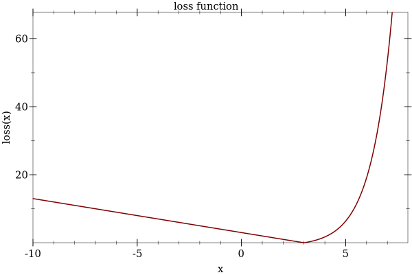
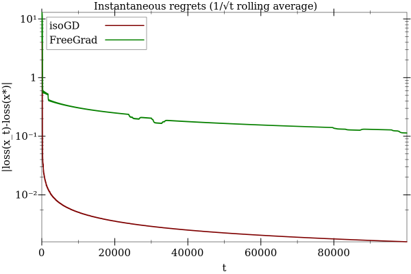
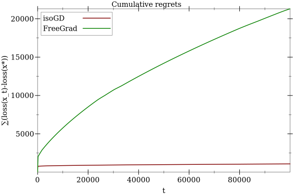
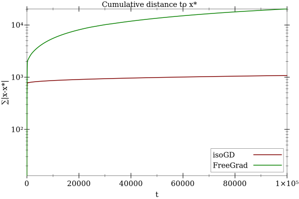
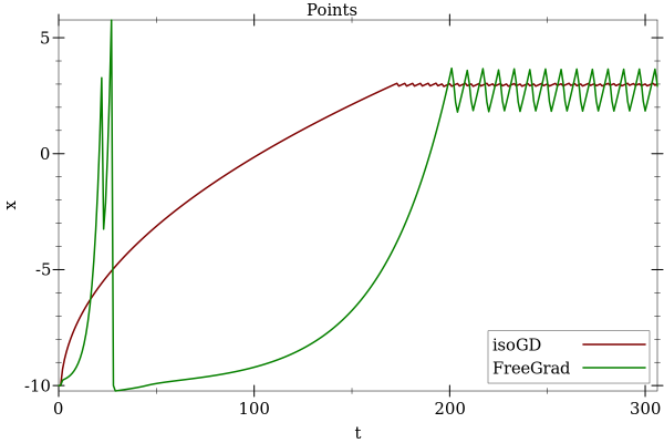
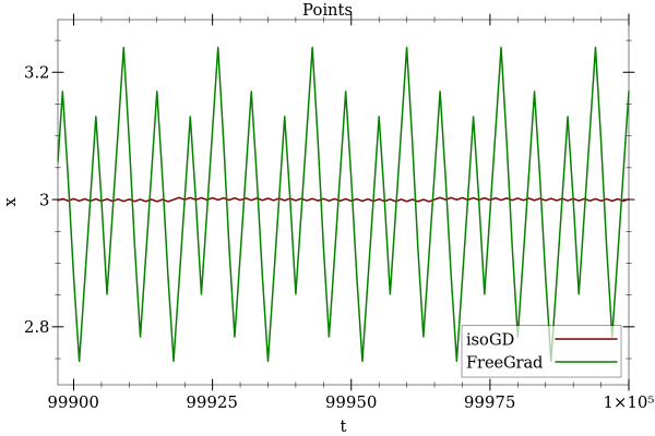
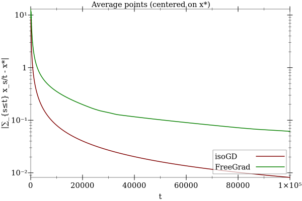
Figure 2: Behaviour of isoGD ($q=1$) and FreeRange on performing gradient descent on $\ell(\bm{x})=\bm{x}^{*}-\bm{x}$ if $\bm{x}<\bm{x}^{*}$ and $\ell(\bm{x})=\exp(\bm{x}-\bm{x}^{*})-1$ otherwise. Note the log scales on some of the y-axis.

Example 43 (MD on the simplex).

When the Bregman divergence is the the relative entropy $B_{R}(a,b)=\sum_{i\in[N]}a_{i}\ln(a_{i}/b_{i})$, and $\mathcal{X}=\Delta_{\text{p}}(N)$ is the probability simplex, then $\|\cdot\|=\|\cdot\|_{1}$ and $\|\cdot\|_{*}=\|\cdot\|_{\infty}$, $\phi_{1}\leq\ln N$, and $D=2$ so taking $q=\ln N$ gives

$$\mathcal{R}_{T}(\bm{x}^{*})\leq 2\sqrt{\ln N\sum_{t\in[T]}\|\ell_{t}\|_{\infty}^{2}}+(4+\sqrt{2\ln N})\max_{t\in[T]}\|\ell_{t}\|_{\infty}\,.$$

See also Appendix E for a more adaptive so-called second order bound with excess losses like AdaHedge (de Rooij et al., 2014) but with a Mirror-Descent-style projection, and a loss translation lemma on the simplex, which applies to the bound above. ∎

Appendix D ISOML-PROD DETAILED PROOF

Proof of 24.

Recall Eq. 12:

$$\mathcal{R}_{i,T}=\sum_{t\in[T]}(\bar{\ell}_{t}-\ell_{i,t})\leq\left(1+\frac{\ln\bm{x}_{i,T+1}}{\ln N}\right)\Delta_{i,T}\,.$$

We proceed to bound $\bm{x}_{i,T+1}$ and $\Delta_{i,T}$ in turn.

Bounding $\bm{x}_{i,T+1}$.

For $t\notin\mathcal{T}_{\emptyset}$, combining with Eq. 11 and the online correction Eq. 3 we have

$$\sum_{j\in[N]}\bm{x}_{j,t+1} \leq\sum_{j\in[N]}\left[\bm{x}_{j,t}(1+\eta_{j,t-1}(\bar{\ell}_{t}-\ell_{j,t}))+\frac{\delta_{j,t}}{\Delta_{j,t}}\bm{x}_{j,1}\right]$$

$$=\sum_{j\in[N]}\bm{x}_{j,t}+\underbrace{\sum_{j\in[N]}\bm{x}_{j,t}\eta_{j,t-1}\bar{\ell}_{t}-\sum_{j\in[N]}\bm{x}_{j,t}\eta_{j,t-1}\ell_{j,t}}_{=0\text{ by \lx@cref{creftype~refnum}{eq:mlprod_barloss}}}+\sum_{j\in[N]}\frac{\delta_{j,t}}{\Delta_{j,t}}\bm{x}_{j,1}$$

$$\leq\sum_{j\in[N]}\bm{x}_{j,t}+\sum_{j\in[N]}\frac{\delta_{j,t}}{\Delta_{j,t}}\bm{x}_{j,1}\,.$$ (15)

Observe that Eq. 15 holds straightforwardly also for $t\in\mathcal{T}_{\emptyset}$ since $\bm{x}_{t^{\prime}}=\bm{x}_{t}$—this would not be the case if null updates were not performed on all coordinates at once. Hence, by summing over $t\in[T]$ and telescoping we have, using $\bm{x}_{j,1}=1$,

$$\sum_{j\in[N]}\bm{x}_{j,T+1} \leq N+\sum_{j\in[N]}\sum_{t\in[T]}\frac{\delta_{j,t}}{\Delta_{j,t}}\,.$$

Note that if $\Delta_{j,t}=0$, necessarily by Eq. 3 we have $\bm{x}_{t+1}=\bm{x}_{j,t^{\prime}}=\bm{x}_{j,1}$, so we can choose $\delta_{j,t}/\Delta_{j,t-1}=0$. Define $C_{j,T}=\sum_{t\in[T]}\frac{\delta_{j,t}}{\Delta_{j,t}}$, then

$$\bm{x}_{i,T+1}\leq\sum_{j\in[N]}\bm{x}_{j,T+1}\leq N+N\max_{j\in[N]}C_{j,T}\,.$$

Bounding $\Delta_{i,T}$.

Recall that $\tau=\max\mathcal{T}_{\emptyset}$ is the last step where a null update is performed, and note that $\tau\geq 1$ when $T\geq 1$ unless the losses are 0. Let $\mu\in[N]$ be such that $\eta_{\mu,\tau-1}|\bar{\ell}_{t}-\ell_{\mu,t}|>1/2$ ($\mu$ necessarily exists by definition of $\mathcal{T}_{\emptyset}$). This implies that $\eta^{-1}_{\mu,\tau-1}<2S$, and thus $\Delta_{\mu,\tau-1}<2S\ln N$. Therefore, since null updates are performed on all coordinates at the same time with $\delta_{\cdot,t}=s_{t}$ for $t\in\mathcal{T}_{\emptyset}$, for all $i\in[N]$ we have

$$\sum_{t\in\mathcal{T}_{\emptyset}}\delta_{i,t}\ =\ \sum_{t\in\mathcal{T}_{\emptyset}}\delta_{\mu,t}\ \leq\ \Delta_{\mu,\tau}\ =\ \Delta_{\mu,\tau-1}+\delta_{\mu,\tau}\ \leq\ 2S\ln N+S\,.$$ (16)

Now define

$$\forall t\notin\mathcal{T}_{\emptyset}:\quad\forall y>0:\hat{\delta}_{t}(y) =\frac{qr_{i,t}^{2}}{2y}\,,\quad\forall y\leq 0:\hat{\delta}_{t}(y)=\infty\,, \forall t\in\mathcal{T}_{\emptyset}:\hat{\delta}_{t}(.) =0\,.$$

Also define $A_{t}=\sum_{u\in\mathcal{T}_{\emptyset}\cap[t]}\delta_{i,s}$. Then by Lemma 46, for $t\notin\mathcal{T}_{\emptyset}$,

$$\delta_{t}\ \leq\ \hat{\delta}_{t}(\Delta_{t-1}-q|r_{i,t}|)\ =\ \hat{\delta}_{t}((\Delta_{t}-A_{t})-\delta_{t}-q|r_{i,t}|+A_{t})\ \leq\ \hat{\delta}_{t}((\Delta_{t}-A_{t})-\delta_{t}-q|r_{i,t}|)\,.$$

Define $\tilde{\Delta}_{t}=\Delta_{t}-A_{t}$, then for all $t\notin\mathcal{T}_{\emptyset}$, $\tilde{\Delta}_{t}=\tilde{\Delta}_{t-1}+\delta_{t}$ with $\delta_{t}\leq\hat{\delta}_{t}(\tilde{\Delta}_{t}-\delta_{t}-q|r_{i,t}|)$ and for $t\in\mathcal{T}_{\emptyset},\tilde{\Delta}_{t}=\tilde{\Delta}_{t-1}+0=\tilde{\Delta}_{t}+\hat{\delta}_{t}(\tilde{\Delta}_{t})$. Therefore, by Lemma 13, with the isotuning sequence $(\hat{\Delta},\hat{\delta})$, and using Lemma 10 on $\hat{\Delta}_{T}$,

$$\tilde{\Delta}_{T} \leq\hat{\Delta}_{T}+\max_{t\in[T]}\{\delta_{t}+q|r_{i,t}|\}\,,$$

$$\Delta_{T} \leq\sqrt{q\sum_{t\notin\mathcal{T}_{\emptyset}}r_{i,t}^{2}}+\max_{t\notin\mathcal{T}_{\emptyset}}\{\delta_{t}+q|r_{i,t}|\}+A_{T}\ \leq\ \sqrt{V_{i,T}\ln N}+S/5+S\ln N+2S\ln N+S$$

where $A_{T}$ is bounded in Eq. 16, and $\delta_{t}=r_{i,t}\left(1-\frac{1}{u}\ln(1+u)\right)$ with $u=\eta_{i,t-1}r_{i,t}\leq 1/2$ can be bounded by $r_{i,t}/5$.

Finally.

We can now put it all together:

$$\mathcal{R}_{i,T} \leq\left(1+\frac{\ln\left(N+N\max_{j\in[N]}C_{j,T}\right)}{\ln N}\right)\left(\sqrt{V_{i,T}\ln N}+3S\ln N+\tfrac{6}{5}S\right)$$

$$\leq\left(2+\frac{\ln\left(1+\max_{j\in[N]}C_{j,T}\right)}{\ln N}\right)\left(\sqrt{V_{i,T}\ln N}+S(\tfrac{6}{5}+3\ln N)\right)\,.$$

Let $t_{0}=\min\{t\in[T]:\Delta_{j,t}>0\}$, then for all $\theta\in\{t_{0},\dots,T\}$,

$$C_{j,T}=\sum_{t\in[T]}\left(1-\frac{\Delta_{j,t-1}}{\Delta_{j,t}}\right)=\sum_{t=t_{0}+1}^{T}\left(1-\frac{\Delta_{j,t-1}}{\Delta_{j,t}}\right)=\sum_{t=t_{0}+1}^{\theta}\underbrace{\left(1-\frac{\Delta_{j,t-1}}{\Delta_{j,t}}\right)}_{\leq 1}+\sum_{t=\theta}^{T}\ln\frac{\Delta_{j,t}}{\Delta_{j,t-1}}\leq\theta-t_{0}+\ln\frac{\Delta_{j,T}}{\Delta_{j,\theta}}$$

where we used $1-1/x\leq\ln x$ and telescoping. Hence,

$$C_{j,T}\leq\min_{\theta\in\{t_{0},\dots,T\}}\theta-t_{0}+\ln\frac{\Delta_{j,T}}{\Delta_{j,\theta}}\,.$$

From this we can deduce all the following simultaneously:

$$C_{j,T} \leq T\,, \text{with }\theta=T\,,$$

$$C_{j,T} \leq o(1)+\ln ST \text{with }\theta=\operatorname*{argmin}_{t\in[T]}\left\{\Delta_{j,t}\geq\frac{\Delta_{j,T}}{ST}\right\}\text{since }\Delta_{j,T}=O(\sqrt{ST}\ln T)\,,$$

$$\text{then }\frac{\Delta_{j,T}}{ST}=o(1),\text{ and thus }\theta=t_{0}+o(1)\,,$$

$$C_{j,T} \leq\tau+\ln\frac{ST}{s_{\tau}} \text{ with }\theta=\tau=\max\mathcal{T}_{\emptyset}\text{ since }\Delta_{j,\tau}\geq\delta_{j,\tau}=s_{\tau}$$

$$\text{ and }\Delta_{j,T}\leq ST\text{ since }\delta_{j,t}\leq S\text{ for all }t\in[T]\,.\qed$$

Remark 44.

With a slight modification of Algorithm 4, we can obtain a variant of the Bernstein Optimal Aggregation (BOA) algorithm (Wintenberger, 2016) (see Footnote 5 in main text) with online correction and null updates and prove the same bound as for isoML-Prod under the same constraints. Replace Eq. 11 with

$$\forall i\in[N]:\bm{x}_{i,t^{\prime}} =\bm{x}_{i,t}f(\eta_{i,t-1}r_{i,t}) \text{ with }f(y) =\exp\left(y-\frac{y^{2}/2}{1-|y|}\right)\,.$$

Recall that $\phi_{i}(\bm{x})=-\ln\bm{x}_{i}$ and $\mathcal{X}=[0,\infty)^{N}$. To satisfy Eq. 5 we take

$$\delta_{i,t}=\delta^{*}_{i,t}=\left(\frac{1}{\eta_{i,t-1}}(\phi_{i,t^{\prime}}-\phi_{i,t})+r_{i,t}\right)_{\!+}=\eta_{i,t-1}\frac{r_{i,t}^{2}/2}{1-\eta_{i,t-1}|r_{i,t}|}\,.$$

We also need to show that Eq. 15 still holds: We do this by reducing it to the isoML-Prod case by using $f(y)\leq 1+y$ for $|y|<1$ (from Lemma 46) with $y=\eta_{i,t-1}r_{i,t}$; though as for isoML-Prod we enforce $|y|\leq 1/2$ to bound $\max_{t}\delta_{t}\leq S$ (which is slightly worse than $S/5$ for isoML-Prod). This constraint means that we need to perform null updates in the same conditions as for isoML-Prod, and we also still need null updates to be performed on all coordinates at the same time. Therefore the bound of 24 holds also for this variant of BOA. Note that Lemma 46 also saves a factor $\sqrt{2}$ compared to prior work where $\exp(y-y^{2})$ is used instead of $\exp(y-y^{2}/(2(1-|y|)))$. ∎

Remark 45.

It is straightforward to adapt the proof to allow for different initial weights $\bm{x}_{i,1}$ that may depend on $i$, as well as extending to a growing number of experts (Mourtada and Maillard, 2017). For example, if we can ensure that $\sum_{i\in[N]}\bm{x}_{i,1}\leq 1$ (and still $\bm{x}_{i,1}\geq 0$), then we would have $\phi_{i,1}=\ln\frac{1}{\bm{x}_{i,1}}$ (instead of 0 in Eq. 12) but from Eq. 15 we have by telescoping

$$\bm{x}_{i,T+1}\leq\sum_{j\in[N]}\bm{x}_{j,1}+\sum_{j\in[N]}\bm{x}_{j,1}C_{j,T}\leq 1+\langle\bm{x}_{1},C_{\cdot,T}\rangle$$

and setting $q_{i}=\ln\frac{1}{\bm{x}_{i,1}}=\phi_{i,1}$ we obtain the regret bound, using $\mathcal{R}_{T}(\bm{x}^{*})=\langle\bm{x}^{*},(\mathcal{R}_{i,T})_{i\in[N]}\rangle$ on the simplex,

$$\mathcal{R}_{T}(\bm{x}^{*}) \leq\sum_{i}\bm{x}^{*}_{i}\left(1+\frac{\phi_{i,1}}{q_{i}}+\frac{\ln(1+\langle\bm{x}_{1},C_{\cdot,T}\rangle)}{q_{i}}\right)\left(\sqrt{q_{i}V_{i,T}}+3Sq_{i}+2S\right)$$

$$\leq\left(2+\frac{\ln(1+\langle\bm{x}_{1},C_{\cdot,T}\rangle)}{\min_{i}\ln\frac{1}{\bm{x}_{i,1}}}\right)\left(\sqrt{\text{H}(\bm{x}^{*},\bm{x}_{1})\sum_{i}\bm{x}^{*}_{i}V_{i,T}}+3S\text{H}(\bm{x}^{*},\bm{x}_{1})+2S\right)\,,$$

where $\text{H}(\bm{x}^{*},\bm{x}_{1})=\sum_{i}\bm{x}^{*}_{i}\ln\frac{1}{\bm{x}_{i,1}}$ is the cross-entropy of $\bm{x}^{*}$ and $\bm{x}_{1}$ (and is equal to the relative entropy $\text{RE}(\bm{x}^{*}\|\bm{x}_{1})$ plus the constant entropy term $\text{H}(\bm{x}^{*},\bm{x}^{*})$), and we used Cauchy-Schwarz on $\sum_{i}\bm{x}^{*}_{i}\sqrt{q_{i}V_{i,T}}=\sum_{i}\sqrt{\bm{x}^{*}_{i}q_{i}}\sqrt{\bm{x}^{*}_{i}V_{i,T}}\leq\sqrt{\sum_{i}\bm{x}^{*}_{i}q_{i}}\sqrt{\sum_{i}\bm{x}^{*}_{i}V_{i,T}}$. Finally, note that $C_{j,T}$ is independent of $q_{j}$. We recover exactly the bound of 24 when $\bm{x}_{i,1}=1/N$. ∎

Lemma 46.

For all $x\in(-1,1)$,

$$\ln(1+x)\geq x-\frac{x^{2}}{2(1-|x|)}\,.\qed$$

Proof.

For $x\in[0,1)$, define $g_{+}(x)=\tfrac{1}{2}x^{2}+(1-x)(\ln(1+x)-x)$. Then $g_{+}^{\prime}(x)=x-(\ln(1+x)-x)+\frac{1-x}{1+x}-(1-x)\geq 0$, hence $g_{+}$ is increasing on $[0,1)$ and since $g_{+}(0)=0$ then $g_{+}(x)\geq 0$ for all $x\in[0,1)$.

Similarly, for $x\in(-1,0]$, define $g_{-}(x)=\tfrac{1}{2}x^{2}+(1+x)(\ln(1+x)-x)$. Then $g_{-}^{\prime}(x)=x+(\ln(1+x)-x)+1-(1+x)=\ln(1+x)-x\leq 0$ and since $g_{-}(0)=0$ then $g_{-}(x)\geq 0$ for all $x\in(-1,0]$, which concludes the proof. ∎

Appendix E ADAHEDGE, MIRROR-DESCENT STYLE

As mentioned before, the present paper is building upon the balancing of the regret idea of de Rooij et al. (2014) for AdaHedge. We show how to build a variant of AdaHedge that uses Mirror Descent-style projection with online correction based on Algorithm 1 without null updates, and straightforwardly recover the same regret bound with our tools, with a slight generalization.

We assume $\mathcal{X}=\Delta_{\text{p}}(N)$. Recall that the loss of the algorithm is $\bar{\ell}_{t}=\sum_{i\in[N]}\bm{x}_{i,t}\ell_{i,t}$ with $\ell_{t}\in{\mathbb{R}}^{N}$ and the instantaneous regret is $r_{t}=\langle\bm{x}_{t}-\bm{x}^{*},\ell_{t}\rangle$. Define, for some unknown $T\in{\mathbb{N}}_{1}$,

$$L =\max_{t\in[T],i\in[N]}|\ell_{i,t}|\,, S =\max_{t\in[T],i\in[N]}|\bar{\ell}_{t}-\ell_{i,t}|\,,$$

$$u_{t} =\sum_{i}\bm{x}_{i,t}(\ell_{i,t}-m_{t})^{2}\,, U_{T} =\sum_{t\in[T]}u_{t}\,, v^{\prime}_{t} =\sum_{i}\bm{x}_{i,t}(\bar{\ell}_{t}-\ell_{i,t})^{2}\,, V^{\prime}_{t} =\sum_{t\in[T]}v^{\prime}_{t}\,.$$

de Rooij et al. (2014) prove the scale-free bound of AdaHedge by first analyzing the regret for $[0,1]$ losses and then showing that the algorithm outputs predictions that are invariant to any rescaling of the losses.

Theorem 47 (Theorem 6, de Rooij et al. (2014), rescaled).

The regret of AdaHedge is bounded by

$$\mathcal{R}_{i,T}\leq 2\sqrt{V^{\prime}_{T}\ln N}+S^{\prime}\left(2+\tfrac{4}{3}\ln N\right)\,.$$

where $S^{\prime}=\max_{t\in[T]}(\max_{i\in[N]}\ell_{i,t}-\min_{j\in[N]}\ell_{j,t})$. ∎

This regret bound has the nice property of being invariant to any translation of the losses. However, surprisingly, it turns out that on the simplex non-translation invariant bounds have better properties since they can always be made translation invariant, while the converse may not hold:

Lemma 48 (Loss translation on the simplex).

Let $\mathcal{X}=\Delta_{\text{p}}(N),\ell_{t}\in{\mathbb{R}}^{N},\forall t\in{\mathbb{N}}_{1}$. For all $\bm{x}^{*}\in\mathcal{X}$, if an algorithm $\mathcal{A}$ sequentially predicts $\bm{x}_{t}$ and has a regret of the form

$$\mathcal{R}_{T}(\bm{x}^{*})\leq f(\ell_{1},\ell_{2},\dots)$$

then for all sequentially available $m_{t}\in{\mathbb{R}}$, algorithm $\mathcal{A}$ fed with the translated losses $\tilde{\ell}_{t}=\ell_{t}-m_{t}$ achieves the regret

$$\mathcal{R}_{T}(\bm{x}^{*})=\sum_{t}\langle\bm{x}_{t}-\bm{x}^{*},\ell_{t}\rangle\leq f(\ell_{1}-m_{1},\ell_{2}-m_{2},\dots)\,.$$

Proof.

Simply observe that on the simplex the regret is translation invariant: $\langle\bm{x}_{t}-\bm{x}^{*},\ell_{t}-m_{t}\rangle=\langle\bm{x}_{t}-\bm{x}^{*},\ell_{t}\rangle$. ∎

In particular when $m_{t}=\bar{\ell}_{t}$ the regret bound becomes translation invariant. See also Chen et al. (2021) for a coordinate-wise generalization of this property and additional discussion of its benefits.

We now describe the isoHedge algorithm. We use Assumption 1, and we take and $\phi(\bm{x})=\text{RE}(\bm{x}^{*}\|\bm{x})$. Define the update rule, for all $i\in[N]$ and for all $t\in{\mathbb{N}}_{1}$:

$$\bm{x}_{i,1} =\frac{1}{N}\,,$$

$$\bm{x}_{i,t^{\prime}} =\bm{x}_{i,t}\frac{\exp(-\eta_{t-1}\ell_{i,t})}{\sum_{j\in[N]}\bm{x}_{j,t}\exp(-\eta_{t-1}\ell_{j,t})}$$ (AdaHedge update and ‘projection’, MD style)

and we also use the online correction of Eq. 3. Null updates are unnecessary in this case because the update is always valid and $\delta_{t}$ will always be bounded by the largest loss. Define $q=\ln N$, and we define $\delta_{t}$ as tightly as possible from Eq. 5:

$$\delta_{t} =\delta^{*}_{t}=\left(\frac{1}{\eta_{t-1}}\ln\frac{\bm{x}_{i,t}}{\bm{x}_{i,t^{\prime}}}+r_{t}\right)_{\!+}=\frac{1}{\eta_{t-1}}\ln\left(\sum_{j\in[N]}\bm{x}_{j,t}\exp(-\eta_{t-1}\ell_{j,t})\right)+\bar{\ell}_{t}\,.$$ (17)

Note that the definition of $\delta_{t}$ is independent of the coordinate $i$. See Algorithm 5.

⬇

def isoHedge():

$\bm{x}_{1}=\left(\frac{1}{N},\dots,\frac{1}{N}\right)$

$\Delta_{0}=0$

for t = 1, 2, ...:

predict $\bm{x}_{t}$ ; observe $\ell_{t}$

choose $m_{t}\in{\mathbb{R}}$ # can be ${\color[rgb]{.8,.4,0}\bar{\ell}_{t}}$

$\eta=q/\Delta_{t-1}$ # ${\color[rgb]{.8,.4,0}\eta_{t-1}}$

$Z=\sum_{j\in[N]}\bm{x}_{j,t}\exp(\eta(m_{t}-\ell_{j,t}))$

for $i\in[N]$:

$\bm{x}_{i,t^{\prime}}=\frac{1}{Z}\bm{x}_{i,t}\exp(\eta(m_{t}-\ell_{i,t}))$ # AdaHedge update, MD style, projection = normalization

$\delta_{t}=\frac{1}{\eta}\ln Z+\bar{\ell}_{t}$ # AdaHedge’s mixability gap

$\Delta_{t}=\Delta_{t-1}+\delta_{t}$ # isotuning

$\bm{x}_{t+1}=\bm{x}_{t^{\prime}}\frac{\Delta_{t-1}}{\Delta_{t}}+\frac{\delta_{t}}{\Delta_{t}}\bm{x}_{1}$ # online correction

Algorithm 5 Instance of Algorithm 1 for AdaHedge with Mirror-Descent-style projection, online correction and isotuning (no null updates). Note that if $\Delta_{t-1}=0$, the limit $\eta^{-1}_{t-1}\to 0$ gives $\delta_{t}=\max_{i\in[N]}(\bar{\ell}_{t}-\ell_{i,t})$, and the online correction implies that $\bm{x}_{t+1}=\bm{x}_{1}$.

Theorem 49.

For all sequentially chosen $\{m_{t}\}_{t}\in{\mathbb{R}}^{T}$ the regret of isoHedge in Algorithm 5 after $T$ rounds is at most

$$\mathcal{R}_{T}(\bm{x}^{*})\leq 2\sqrt{U_{t}\ln N}+2S+\tfrac{2}{3}L\ln N\,.$$

In particular with $m_{t}=\bar{\ell}_{t}$, the regret is bounded by

$$\mathcal{R}_{T}(\bm{x}^{*})\leq 2\sqrt{V^{\prime}_{t}\ln N}+2S+\tfrac{2}{3}S\ln N\,.\qed$$

Proof.

We prove for $m_{t}=0,\forall t$ and apply Lemma 48.

As usual, we need to express $\delta_{t}$ as a function of $\Delta_{t}$. Define $\hat{\delta}_{t}(x)=qu_{t}/(2x)$ for $x>0$ and $\hat{\delta}_{t}(x)=\infty$ otherwise. From Corollary 52, we know that $e^{x}\leq 1+x+\frac{x^{2}/2}{1-x/3}$ for $x<3$ and so, with $\ln(1+x)\leq x$,

$$\delta_{t}\ \leq\ \frac{1}{\eta_{t-1}}\ln\left(\sum_{j}\bm{x}_{j,t}\left(1-\ell_{j,t}+\frac{\eta_{t-1}^{2}\ell_{j,t}^{2}/2}{1+\eta_{t-1}\ell_{j,t}/3}\right)\right)+\bar{\ell}_{t}$$

$$\leq\frac{\eta_{t-1}u_{t}/2}{1-\eta_{t-1}L/3}\ =\ \frac{qu_{t}/2}{\Delta_{t-1}-qL/3}\ =\ \frac{qu_{t}/2}{\Delta_{t}-\delta_{t}-qL/3}$$

which is valid at least when $\Delta_{t}-\delta_{t}-qL/3>0$, and thus $\delta_{t}\leq\hat{\delta}_{t}(\Delta_{t}-\delta_{t}-qL/3)$ for all $t\in[T]$. Therefore, using Lemma 13, let $(\hat{\Delta},\hat{\delta})$ be an isotuning sequence, then

$$\Delta_{T}\leq\hat{\Delta}_{T}+\max_{t\in[T]}\{\delta_{t}+qL/3\}\leq\sqrt{q\sum_{t\in[T]}u_{t}}+S+qL/3$$

by Lemma 10 and using $\delta_{t}\leq S$ from Eq. 17. The result follows from Lemma 12, since with $\phi_{1}=\ln N=q$ we have $\mathcal{R}_{i,T}\leq 2\Delta_{T}$. ∎

Observe that by contrast to the original analysis of AdaHedge, our analysis applies directly to losses in ${\mathbb{R}}^{N}$. Furthermore, the only application-specific difficulty is to bound $\delta_{t}$.

Remark 50.

One difference between isoHedge (when $m_{t}=\bar{\ell}_{t}$) and AdaHedge is that for $t=2$ AdaHedge predicts at a corner of the probability simplex like Follow The Leader (FTL) (de Rooij et al., 2014), while isoHedge predicts at the ‘center’ $(1/N,1/N,\dots)$. This latter behaviour is also the choice made by SOLO FTRL (Orabona and Pál, 2018), which deals with both bounded and unbounded domains—where playing at a corner is not always possible or even desirable. In particular, when losses are gradients, playing at a corner may lead to unbounded or infinite losses, e.g., $\ell_{i,t}=\frac{\partial(-\log\langle\bm{x}_{t},f_{t}\rangle)}{\partial\bm{x}_{i,t}}$ for some $f_{t}$. ∎

The following results are technical lemmas used in the proof of 49. A similar result can be extracted from the proofs of de Rooij et al. (2014).

Lemma 51.

For all $x\in{\mathbb{R}}$, $(e^{x}-x-1)(1-x/3)\leq x^{2}/2$. ∎

Proof.

Let

$$f(x) =(e^{x}-x-1)(1-x/3)-x^{2}/2$$

$$=e^{x}(3-x)/3+(x+1)(x/3-1)-x^{2}/2\,,$$

$$f^{\prime}(x) =e^{x}(2-x)/3-x/3-2/3\,,$$

$$f^{\prime\prime}(x) =e^{x}(1-x)/3-1/3\,,$$

$$f^{\prime\prime\prime}(x) =-xe^{x}/3\,.$$

Notice that $f(0)=f^{\prime}(0)=f^{\prime\prime}(0)=0$ and all functions above are continuous on ${\mathbb{R}}$. Therefore a Taylor expansion at 0 with Lagrange remainder gives $f(x)=-x^{3}ye^{y}/3$ for some $y$ between $x$ and 0 and thus $f(x)\leq 0$ for all $x\in{\mathbb{R}}$, which proves the result. ∎

Corollary 52.

For all $x<3$, $e^{x}\leq 1+x+\frac{x^{2}/2}{1-x/3}$. ∎

Proof.

Follows from Lemma 51. ∎

Appendix F SOFT-BAYES REVISITED

Soft-Bayes (Orseau et al., 2017) is an algorithm for the universal portfolio problem (Cover, 1991), with running time $O(N)$ per step for $N$ experts and a regret bound of $O(\sqrt{NT\ln N})$. A variant is also given with a better bound of $O(\sqrt{mT\ln N})$ where $m$ is the number of experts in hindsight that have been ‘good’ at least once after $T$ steps. While not changing the computational complexity of the algorithm, this variant requires keeping track of these $m$ experts online with an array of size $N$, thus making the algorithm less simple and makes the bound dependent on the specifics of the tracking algorithm.

We show how isotuning can be used to obtain a regret bound of $O(\sqrt{mT\ln N})$ without having to keep track of $m$, just by using the prescribed isotuning learning rate. We do not need null updates as we can bound $\max_{t}\delta_{t}$ directly.

We are in the online convex optimization setting, where $\mathcal{X}$ is the probability simplex of $N$ coordinates, and $\ell_{t}(\bm{x})=-\ln\langle\bm{x},p_{t}\rangle$ where $p_{t}\in[0,\infty)^{N}$.

Let $\mathcal{N}_{T}\in\operatorname*{argmin}_{S\subseteq[N]}\{|S|\mid\forall t\in[T]:S\cap\operatorname*{argmax}_{i\in[N]}\{p_{i,t}\}\neq\emptyset\}$ be the smallest subset of $[N]$ such that at each step $t$ at least one of the best experts at step $t$ is in this subset. Ties are broken arbitrarily. Note that neither $\mathcal{N}_{T}$ nor $|\mathcal{N}_{T}|$ need to be tracked by the algorithm, by contrast to the original work, which allows us to compete against a better subset in hindsight.

The core update of the Soft-Bayes algorithm is as follows (note that the notation for the index of the learning rate is offset by one compared to the notation of the original paper, to be aligned with the notation of the current paper). For all $i\in[N]$ and $t\in[T]$,

$$\bm{x}_{i,1} =\frac{1}{N}\,,$$

$$\bar{p}_{t} =\langle\bm{x}_{t},p_{t}\rangle\,,$$ (mixture prediction)

$$\bm{x}_{i,t^{\prime}} =\bm{x}_{i,t}\left(1-\eta_{t-1}+\eta_{t-1}\frac{p_{i,t}}{\bar{p}_{t}}\right)\,,$$ (Soft-Bayes update) (18)

The online correction of Eq. 3 is also applied (as in the original work), but not null updates. See Algorithm 6, and note that by contrast to the original algorithm, it does not indeed require keeping track of $m$.

⬇

def isoSoft-Bayes($N\geq 2$):

$\Delta_{0}=2\ln N$

$\bm{x}_{1}=\{\frac{1}{N},\frac{1}{N},\dots,\frac{1}{N}\}$

for $t=1,2,\dots$:

predict $\bm{x}_{t}$; observe $p_{t}$ # loss is ${\color[rgb]{.8,.4,0}-\ln\bar{p}_{t}}$

$\bar{p}_{t}=\langle\bm{x}_{t},p_{t}\rangle$

$\eta=\frac{\ln N}{\Delta_{t-1}}$ # ${\color[rgb]{.8,.4,0}\eta_{t-1}}$

$\forall i\in[N]:\bm{x}_{i,t^{\prime}}=\bm{x}_{i,t}\left(1-\eta+\eta\frac{p_{i,t}}{\bar{p}_{t}}\right)$ # Soft-Bayes update

$\delta_{t}=\max_{i\in[N]}\ln\left(1+\frac{\eta}{1-\eta}\frac{p_{i,t}}{\bar{p}_{t}}\right)$

$\Delta_{t}=\Delta_{t-1}+\delta_{t}$ # isotuning

$\bm{x}_{t+1}=\bm{x}_{t^{\prime}}\frac{\Delta_{t-1}}{\Delta_{t}}+\frac{\delta_{t}}{\Delta_{t}}\bm{x}_{1}$ # online correction

Algorithm 6 The Soft-Bayes algorithm with isotuning with regret $O(\sqrt{mT\ln N})$ where $m$ is the number of ‘good’ experts. Null updates are not used as the additive term $\max_{t}\delta_{t}$ is well bounded.

First we recall a central lemma of the original paper:

Lemma 53 (Lemma 4, Orseau et al. (2017)).

Let $\bm{x}\in\mathcal{X}$ and $b\in[0,\infty)^{N}$, then for all $\eta\in(0,1)$,

$$\ln\sum_{i\in[N]}\bm{x}_{i}b_{i}\leq\frac{1}{\eta}\sum_{i\in[N]}\bm{x}_{i}\ln(1-\eta+\eta b_{i})+\max_{i\in[N]}\ln\left(1+\frac{\eta}{1-\eta}b_{i}\right)\,.\qed$$

Define for all $t\in[T]$ (note that this slightly differs from Assumption 1),

$$q =\ln N\,, \Delta_{t} =\frac{q}{\eta_{t}}\,, \Delta_{0} =2q\,, \Delta_{t} =\Delta_{t-1}+\delta_{t}\,.$$

Theorem 54.

The regret of isoSoft-Bayes (Algorithm 6) for all $\bm{x}^{*}\in\mathcal{X}$ is bounded for all $T\in{\mathbb{N}}_{1}$ by

$$\mathcal{R}_{T}(\bm{x}^{*})\leq 4\sqrt{mT\ln N}+3\ln O(NT)+10m\ln\frac{N}{m}+6\ln N\,.$$

Proof.

Define $\phi(\bm{x})=\sum_{i\in[N]}\bm{x}^{*}_{i}\ln\frac{\bm{x}^{*}_{i}}{\bm{x}_{i}}$ and so we take take $q=\ln N\geq\phi_{1}$. To satisfy Eq. 5,

$$\delta^{*}_{t} =\left(\frac{1}{\eta_{t-1}}\sum_{i\in[N]}\bm{x}^{*}_{i}\ln\frac{\bm{x}_{i,t^{\prime}}}{\bm{x}_{i,t}}+\ln\frac{\langle\bm{x}^{*},p_{t}\rangle}{\bar{p}_{t}}\right)_{\!+}$$

$$=\left(-\frac{1}{\eta_{t-1}}\sum_{i\in[N]}\bm{x}^{*}_{i}\ln\left(1-\eta_{t-1}+\eta_{t-1}\frac{p_{i,t}}{\bar{p}_{t}}\right)+\ln\sum_{i\in[N]}\bm{x}^{*}_{i}\frac{p_{i,t}}{\bar{p}_{t}}\right)_{\!+}$$

$$\leq\max_{i\in[N]}\ln\left(1+\frac{\eta_{t-1}}{1-\eta_{t-1}}\frac{p_{i,t}}{\bar{p}_{t}}\right)=:\delta_{t}$$

where we used Lemma 53 on the last line. Hence this definition of $\delta_{t}$ satisfies Eq. 5.

From Lemma 11 and the concavity of the log function, for all $i\in[N]$ we have, using the update rule Eq. 18 on the second line along with $\ln(1+\eta-\eta x)=\ln(1+\frac{\eta}{1-\eta}x)+\ln(1-\eta)$:

$$\Delta_{t}\ln\bm{x}_{i,t+1} \geq\Delta_{t-1}\ln\bm{x}_{i,t^{\prime}}+\delta_{t}\ln\bm{x}_{i,1}$$

$$\Leftrightarrow \Delta_{t-1}\ln\bm{x}_{i,t+1}+\delta_{t}\ln\bm{x}_{i,t+1} \geq\Delta_{t-1}\ln\bm{x}_{i,t}+\Delta_{t-1}\ln\left(1+\frac{\eta_{t-1}}{1-\eta_{t-1}}\frac{p_{i,t}}{\bar{p}_{t}}\right)+\Delta_{t-1}\ln(1-\eta_{t-1})+\delta_{t}\ln\bm{x}_{i,1}$$

$$\Leftrightarrow \ln\left(1+\frac{\eta_{t-1}}{1-\eta_{t-1}}\frac{p_{i,t}}{\bar{p}_{t}}\right) \leq\ln\frac{\bm{x}_{i,t+1}}{\bm{x}_{i,t}}+\frac{\delta_{t}}{\Delta_{t-1}}\ln\frac{\bm{x}_{i,t+1}}{\bm{x}_{i,1}}\underbrace{-\ln(1-\eta_{t-1})}_{\leq\frac{\eta_{t-1}}{1-\eta_{t-1}}=\frac{q}{\Delta_{t-1}-q}}\,,$$

$$\delta_{t}\leq\sum_{i\in\mathcal{N}_{T}}\ln\left(1+\frac{\eta_{t-1}}{1-\eta_{t-1}}\frac{p_{i,t}}{\bar{p}_{t}}\right) \leq\sum_{i\in\mathcal{N}_{T}}\ln\frac{\bm{x}_{i,t+1}}{\bm{x}_{i,t}}+\frac{\delta_{t}}{\Delta_{t-1}}\underbrace{\sum_{i\in\mathcal{N}_{T}}\ln\frac{\bm{x}_{i,t+1}}{\bm{x}_{i,1}}}_{\leq m\ln\frac{N}{m}}+m\frac{q}{\Delta_{t-1}-q}$$ (19)

Define $a=m\ln\frac{N}{m}$, and $b_{t}=\sum_{i\in\mathcal{N}_{T}}\ln\frac{\bm{x}_{i,t+1}}{\bm{x}_{i,t}}$ and we write $b_{1:t}=\sum_{s\in[t]}b_{s}$. Then when $1-a/\Delta_{t-1}>0$ we have

$$\delta_{t}\left(1-\frac{a}{\Delta_{t-1}}\right) \leq b_{t}+\frac{mq}{\Delta_{t-1}-q}\,, \Leftrightarrow \delta_{t} \leq\left(1+\frac{a}{\Delta_{t-1}-a}\right)\left(b_{t}+\frac{mq}{\Delta_{t-1}-q}\right)\,.$$

Define, for all $t\in[T]$,

$$\forall x>0:\hat{\delta}_{t}(x) =\left(1+\frac{a}{x}\right)\left(b_{t}+\frac{mq}{x}\right)\,, \text{and }\forall x\leq 0:\hat{\delta}_{t}(x) =\infty\,.$$

Then, for all $t\in[T]$, since $\hat{\delta}_{t}(\Delta_{t-1}-a)=\infty$ if $1-a/\Delta_{t-1}\leq 0$,

$$\delta_{t}\ \leq\ \hat{\delta}_{t}(\Delta_{t-1}-\max\{a,q\})\ \leq\ \hat{\delta}_{t}\left((\Delta_{t}-\Delta_{0})-\left(\delta_{t}+\max\{a,q\}-\Delta_{0}\right)_{\!+}\right)\,,$$

and observe that $(\Delta_{t}-\Delta_{0})=(\Delta_{t-1}-\Delta_{0})+\delta_{t}$. Let $(\hat{\Delta},\hat{\delta})$ be an isotuning sequence, then by Lemma 13,

$$\Delta_{T}-\Delta_{0} \leq\hat{\Delta}_{T}+\max_{t\in[T]}\left(\delta_{t}+\max\{a,q\}-\Delta_{0}\right)_{\!+}\,,$$

$$\Delta_{T} \leq\hat{\Delta}_{T}+\max_{t\in[T]}\max\{\delta_{t}+\max\{a,q\},\Delta_{0}\}\ \leq\ \hat{\Delta}_{T}+\max_{t\in[T]}\delta_{t}+a+2q\,.$$

By 7 we have

$$\hat{\Delta}_{T}\ \leq\ \inf_{y>0}\left\{y+\sum_{t\in[T]}\left(1+\frac{a}{y}\right)\left(b_{t}+\frac{mq}{y}\right)\right\}\ =\ \inf_{y>0}\left\{y+\frac{ab_{1:T}+mqT}{y}+\frac{amqT}{y^{2}}\right\}+b_{1:T}\ \leq\ 2\sqrt{mqT}+4a\,,$$

where the last inequality is because $b_{1:T}=\sum_{i\in\mathcal{N}_{T}}\ln\frac{\bm{x}_{i,T+1}}{\bm{x}_{i,1}}\leq m\ln\frac{N}{m}=a$, taking $y=\sqrt{a^{2}+mqT}$ and using $\sqrt{u+v}\leq\sqrt{u}+\sqrt{v}$.

We proceed to bound $\max_{t}\delta_{t}$. Using $\bar{p}_{t}\geq\bm{x}_{i,t}p_{i,t}$ and $\eta_{t}/(1-\eta_{t})\leq 2\eta_{t}$ (since $\eta_{0}=\Delta_{0}/q=\tfrac{1}{2}$),

$$\delta_{t}\leq\max_{i}\ln\left(1+2\eta_{t-1}\frac{1}{\bm{x}_{i,t}}\right)=\max_{i}\ln\left(1+2\frac{q}{\Delta_{t-1}}\frac{1}{\bm{x}_{i,t}}\right)$$

Furthermore, since $\bar{p}_{t}\leq\max_{i}p_{i,t}$, then $\delta_{t}\geq\ln(1+\eta_{t-1}/(1-\eta_{t-1}))\geq\eta_{t-1}$. Also, from the online correction Eq. 3, multiplying by $\Delta_{t}$ on both side, we obtain

$$\Delta_{t}\bm{x}_{i,t+1}=\Delta_{t-1}\bm{x}_{i,t^{\prime}}+\delta_{t}\bm{x}_{i,1}\geq\delta_{t}\bm{x}_{i,1}\geq\eta_{t-1}\bm{x}_{i,1}=\frac{q}{N\Delta_{t-1}}$$ (20)

which gives

$$\delta_{t}\leq\ln\left(1+2N\Delta_{t-2}\right)\leq\ln(1+2\Delta_{T})+\ln N\,.$$

Therefore, putting it all together:

$$\Delta_{T}\leq 2\sqrt{mT\ln N}+\ln(1+2\Delta_{T})+5m\ln\frac{N}{m}+3\ln N\,,$$

where $\ln(1+2\Delta_{T})=\ln O(NT)$, and the result follows by $\mathcal{R}_{T}(\bm{x}^{*})\leq 2\Delta_{T}$ from Lemma 12 since $q=\ln N\geq\phi_{1}=\text{RE}(\bm{x}^{*}\|\bm{x}_{1})$. ∎

Remark 55.

We could even exclude $O(\sqrt{mT})$ outliers $\delta_{t}$ from the analysis, since $\delta_{t}\leq\ln O(NT)$. ∎

Remark 56.

54 actually applies to all $m^{\prime}\in\{m,\dots,N\}$ and in particular for $m^{\prime}=N$ for which $m^{\prime}\ln\frac{N}{m^{\prime}}=0$. ∎

Remark 57.

The leading factor 4 is likely due to using the convenient 7, but it seems plausible that a more careful analysis would remove a factor $\sqrt{2}$. ∎

Table of Notation

Notation	Meaning
$[n]$	$\{1,2,\dots,n\}$
$\left(x\right)_{\!+}$	$\max\{0,x\}$
$T$	some (unknown) number of rounds to play
$t$	some round index, usually $t\in[T]$
$N$	number of coordinates/experts
$\mathcal{X}$	convex subset of ${\mathbb{R}}^{N}$
$\Delta_{\text{p}}(N)$	probability simplex with $N$ coordinates
$\bm{x}^{*}$	some competitor point in $\mathcal{X}$
$\bm{x}_{t}$	point in $\mathcal{X}$ played by the algorithm
$\bm{x}_{t^{\prime}}$	algorithm-specific update of $\bm{x}_{t}$ before online correction
$\ell_{t}(\bm{x})$	OCO: loss function at round $t$
$\nabla_{t}$	OCO: $\nabla\ell_{t}$ gradient of the loss function at round $t$
$\ell_{t}$	OLO: in ${\mathbb{R}}^{N}$, loss vector at round $t$; corresponds to $\nabla_{t}$ in OCO
$\ell_{i,t}$	in ${\mathbb{R}}$, loss of coordinate/expert $i$ at round $t$
$\bar{\ell}_{t}$	$\sum_{i}\bm{x}_{i,t}\ell_{i,t}$ loss of the expert algorithm at round $t$
$G$	OCO: $\max_{t\in[T]}\|\nabla_{t}\|_{*}$, largest observed gradient
$L$	OLO: $\max_{t\in[T]}\|\ell_{t}\|_{*}$, largest observed loss
$L_{t}$	FTRL: $\sum_{s\in[t]}\ell_{s}$, cumulative loss
$\mathcal{R}_{T}(\bm{x}^{*})$	cumulative regret of the algorithm compared to $\bm{x}^{*}\in\mathcal{X}$
$r_{t}$	instantaneous regret of the algorithm, usually $\langle\bm{x}_{t}-\bm{x}^{*},\ell_{t}\rangle$ (OLO) or $\ell_{t}(\bm{x}_{t})-\ell_{t}(\bm{x}^{*})$ (OCO)
$r_{i,t}$	$\bar{\ell}_{t}-\ell_{i,t}$ instantaneous regret of the algorithm against expert $i$ at round $t$
$s_{t}$	$\max_{i\in[N]}|r_{i,t}|$
$S$	$\max_{t\in[T]}s_{t}$
$V_{i,T}$	$\sum_{t\in[T]}r_{i,t}^{2}$
$D$	$\max_{(a,b)\in\mathcal{X}^{2}}\|a-b\|$, diameter of $\mathcal{X}$ according to $\|\cdot\|$
$\eta$	learning rate, $\geq 0$
$q$	positive parameter of the algorithms
$\Delta_{t}$	$\Delta_{0}+\sum_{s\in[t]}\Delta_{s}$
$\delta^{*}_{t}$	algorithm-specific quantity, Eq. 4
$\delta_{t}$	algorithm-specific quantity, usually satisfies Eq. 5
$\hat{\delta}_{t}$	non-increasing continuous positive function such that usually $\delta_{t}\leq\hat{\delta}_{t}(\Delta_{t-1})$
$\|\cdot\|$	some norm
$\|\cdot\|_{*}$	dual norm of $\|\cdot\|$
$R$	regularizer, usually 1-strongly convex w.r.t. some norm $\|\cdot\|$ and non-negative
$B_{R}$	Bregman divergence
$\text{RE}(\cdot\|\cdot)$	relative entropy
$\phi$	some convex function
$\left[\!\left[test\right]\!\right]$	indicator function
$g^{\text{low}}_{t}$	lower bound of the domain of some function $g_{t}:(g^{\text{low}}_{t},\infty)\to[0,\infty)$ (Definition 5)
$g^{\inf}_{T}$	$\max_{t\in[T]}\left(g^{\text{low}}_{t}\right)_{\!+}$ for a given sequence of functions $\{g_{t}\}_{t\in[T]}$
$\mathcal{T}_{\emptyset}$	subset of $[T]$ where a null update is performed (Section 3.5)
$\tau$	$\max\mathcal{T}_{\emptyset}$, last round before $T$ a null update is performed (Section 3.5)
$c$	null update factor (Section 3.5)
$\operatorname*{iso}(\cdot,\cdot)$	iso operator (Section 3.1)

References

• Hazan (2016) Elad Hazan. Introduction to online convex optimization. Foundations and Trends® in Optimization, 2(3-4):157–325, 2016.
• Zinkevich (2003) Martin Zinkevich. Online convex programming and generalized infinitesimal gradient ascent. In Proceedings of the Twentieth International Conference on Machine Learning, pages 928–935, 2003.
• Auer et al. (2002) Peter Auer, Nicolò Cesa-Bianchi, and Claudio Gentile. Adaptive and self-confident on-line learning algorithms. Journal of Computer and System Sciences, 64(1):48 – 75, 2002.
• Orabona and Pál (2018) Francesco Orabona and Dávid Pál. Scale-free online learning. Theoretical Computer Science, 716:50–69, 2018.
• Pogodin and Lattimore (2020) Roman Pogodin and Tor Lattimore. On first-order bounds, variance and gap-dependent bounds for adversarial bandits. In Proceedings of The 35th Uncertainty in Artificial Intelligence Conference, volume 115 of Proceedings of Machine Learning Research, pages 894–904. PMLR, 22–25 Jul 2020.
• de Rooij et al. (2014) Steven de Rooij, Tim van Erven, Peter D. Grünwald, and Wouter M. Koolen. Follow the leader if you can, Hedge if you must. J. Mach. Learn. Res., 15(1):1281–1316, January 2014.
• Mhammedi and Koolen (2020) Zakaria Mhammedi and Wouter M. Koolen. Lipschitz and comparator-norm adaptivity in online learning. In Proceedings of Thirty Third Conference on Learning Theory, volume 125 of Proceedings of Machine Learning Research, pages 2858–2887. PMLR, 2020.
• Cesa-Bianchi et al. (2007) Nicolò Cesa-Bianchi, Yishay Mansour, and Gilles Stoltz. Improved second-order bounds for prediction with expert advice. Machine Learning, 66(2-3):321–352, 2007.
• Cesa-Bianchi and Lugosi (2006) Nicolo Cesa-Bianchi and Gabor Lugosi. Prediction, Learning, and Games. Cambridge University Press, New York, NY, USA, 2006.
• Shalev-Shwartz (2007) Shai Shalev-Shwartz. Online learning: Theory, algorithms, and applications. PhD thesis, Hebrew University, Jerusalem, 2007.
• Beck and Teboulle (2003) Amir Beck and Marc Teboulle. Mirror descent and nonlinear projected subgradient methods for convex optimization. Operations Research Letters, 31(3):167–175, 2003.
• Thune et al. (2019) Tobias Sommer Thune, Nicolò Cesa-Bianchi, and Yevgeny Seldin. Nonstochastic multiarmed bandits with unrestricted delays. In Advances in Neural Information Processing Systems 32, pages 6538–6547, 2019.
• Zimmert and Seldin (2020) Julian Zimmert and Yevgeny Seldin. An optimal algorithm for adversarial bandits with arbitrary delays. In Proceedings of the Twenty Third International Conference on Artificial Intelligence and Statistics, volume 108 of Proceedings of Machine Learning Research, pages 3285–3294. PMLR, 2020.
• Orseau et al. (2017) Laurent Orseau, Tor Lattimore, and Shane Legg. Soft-bayes: Prod for mixtures of experts with log-loss. In Proceedings of the 28th International Conference on Algorithmic Learning Theory, volume 76 of Proceedings of Machine Learning Research, pages 372–399, 2017.
• Gaillard et al. (2014) Pierre Gaillard, Gilles Stoltz, and Tim van Erven. A second-order bound with excess losses. In Proceedings of The 27th Conference on Learning Theory, COLT, volume 35 of JMLR Workshop and Conference Proceedings, pages 176–196, 2014.
• Wintenberger (2016) Olivier Wintenberger. Optimal learning with bernstein online aggregation. Machine Learning, 106(1):119–141, 2016.
• Lattimore and Szepesvári (2020) Tor Lattimore and Csaba Szepesvári. Exploration by optimisation in partial monitoring. In Proceedings of Thirty Third Conference on Learning Theory, volume 125 of Proceedings of Machine Learning Research, pages 2488–2515, 09–12 Jul 2020.
• Bartlett et al. (2007) Peter L. Bartlett, Elad Hazan, and Alexander Rakhlin. Adaptive online gradient descent. In Advances in Neural Information Processing Systems 20, pages 65–72, 2007.
• Gyorgy and Szepesvari (2016) Andras Gyorgy and Csaba Szepesvari. Shifting regret, mirror descent, and matrices. In Maria Florina Balcan and Kilian Q. Weinberger, editors, Proceedings of The 33rd International Conference on Machine Learning, volume 48 of Proceedings of Machine Learning Research, pages 2943–2951, New York, New York, USA, 20–22 Jun 2016. PMLR. URL https://proceedings.mlr.press/v48/gyorgy16.html.
• Fang et al. (2020) Huang Fang, Nick Harvey, Victor Portella, and Michael Friedlander. Online mirror descent and dual averaging: keeping pace in the dynamic case. In Hal Daumé III and Aarti Singh, editors, Proceedings of the 37th International Conference on Machine Learning, volume 119 of Proceedings of Machine Learning Research, pages 3008–3017. PMLR, 13–18 Jul 2020. URL https://proceedings.mlr.press/v119/fang20a.html.
• Györfi and Ottucsák (2007) László Györfi and György Ottucsák. Sequential prediction of unbounded stationary time series. IEEE Transactions on Information Theory, 53(5):1866–1872, 2007.
• Chen et al. (2021) Liyu Chen, Haipeng Luo, and Chen-Yu Wei. Impossible tuning made possible: A new expert algorithm and its applications. In Proceedings of Thirty Fourth Conference on Learning Theory, volume 134, pages 1216–1259. PMLR, 15–19 Aug 2021.
• Huang et al. (2021) Jiatai Huang, Yan Dai, and Longbo Huang. Scale-free adversarial multi-armed bandit with arbitrary feedback delays. CoRR, abs/2110.13400, 2021.
• McMahan (2017) H. Brendan McMahan. A survey of algorithms and analysis for adaptive online learning. Journal of Machine Learning Research, 18(90):1–50, 2017.
• Cutkosky (2019) Ashok Cutkosky. Artificial constraints and hints for unbounded online learning. In Proceedings of the Thirty-Second Conference on Learning Theory, volume 99 of Proceedings of Machine Learning Research, pages 874–894. PMLR, 2019.
• Mhammedi et al. (2019) Zakaria Mhammedi, Wouter M Koolen, and Tim Van Erven. Lipschitz adaptivity with multiple learning rates in online learning. In Proceedings of the Thirty-Second Conference on Learning Theory, volume 99 of Proceedings of Machine Learning Research, pages 2490–2511, 2019.
• Cesa-Bianchi et al. (1997) Nicolò Cesa-Bianchi, Yoav Freund, David Haussler, David P. Helmbold, Robert E. Schapire, and Manfred K. Warmuth. How to use expert advice. J. ACM, 44(3):427–485, May 1997.
• Sani et al. (2014) Amir Sani, Gergely Neu, and Alessandro Lazaric. Exploiting easy data in online optimization. In Advances in Neural Information Processing Systems, volume 27. Curran Associates, Inc., 2014.
• van Erven et al. (2011) Tim van Erven, Wouter M Koolen, Steven de Rooij, and Peter Grünwald. Adaptive hedge. In Advances in Neural Information Processing Systems, pages 1656–1664, 2011.
• Herbster and Warmuth (1998a) Mark Herbster and Manfred K. Warmuth. Tracking the best expert. Machine Learning, 32(2):151–178, August 1998a.
• György and Joulani (2021) Andras György and Pooria Joulani. Adapting to delays and data in adversarial multi-armed bandits. In Proceedings of the 38th International Conference on Machine Learning, volume 139, pages 3988–3997. PMLR, 2021.
• Duchi et al. (2011) John Duchi, Elad Hazan, and Yoram Singer. Adaptive subgradient methods for online learning and stochastic optimization. Journal of Machine Learning Research, 12(61):2121–2159, 2011.
• Herbster and Warmuth (1998b) Mark Herbster and Manfred K. Warmuth. Tracking the best regressor. In Proc. 11th Annu. Conf. on Comput. Learning Theory, pages 24–31. ACM Press, New York, NY, 1998b.
• Mourtada and Maillard (2017) Jaouad Mourtada and Odalric-Ambrym Maillard. Efficient tracking of a growing number of experts. In Proceedings of the 28th International Conference on Algorithmic Learning Theory (ALT), volume 76 of Proceedings of Machine Learning Research, pages 517–539, 2017.
• Cover (1991) Thomas M Cover. Universal portfolios. Mathematical finance, 1(1):1–29, 1991.