Model Averaging for Support Vector Machine by Cross-Validation

Abstract

Support vector machine (SVM) is a well-known statistical technique for classification problems in machine learning and other fields. An important question for SVM is the selection of covariates (or features) for the model. Many studies have considered model selection methods. As is well-known, selecting one winning model over others can entail considerable instability in predictive performance due to model selection uncertainties. This paper advocates model averaging as an alternative approach, where estimates obtained from different models are combined in a weighted average. We propose a model weighting scheme and provide the theoretical underpinning for the proposed method. In particular, we prove that our proposed method yields a model average estimator that achieves the smallest hinge risk among all feasible combinations asymptotically. To remedy the computational burden due to a large number of feasible models, we propose a screening step to eliminate the uninformative features before combining the models. Results from real data applications and a simulation study show that the proposed method generally yields more accurate estimates than existing methods.

Keywords: cross-validation, model averaging, model selection, prediction, support vector machine

1 Introduction

Support vector machine (SVM) (Vapnik, 1995; Schölkopf and Smola, 2001) is a well-known statistical technique for handling classification problems in biology, machine learning, medicine and many other fields. An important question for SVM is how to select the covariates (or features) of the model. Many studies have attempted to address this question and come up with a variety of methods. Weston et al. (2000) proposed a scaling method. Guyon et al. (2002) suggested a recursive feature elimination procedure. Some authors have considered regularisation methods within the context of SVM. For example, Bradley and Mangasarian (1998), Zhu et al. (2004) and Wegkamp and Yuan (2011) investigated the properties of a $L_{1}$ penalised SVM; Wang et al. (2006) considered SVMs with $L_{1}$ and $L_{2}$ penalties; Zou and Yuan (2008) considered the $L_{\infty}$ penalised SVM in the presence of prior knowledge in the group information of features; Zhang et al. (2006) and Becker et al. (2011) suggested a non-convex penalty in the application of gene selection; and Park et al. (2012) and Zhang et al. (2016b) investigated the oracle property of the SCAD-penalised SVM with a fixed number of covariates under a class of non-convex penalties. As well, Zhang et al. (2016c) developed a consistent information criterion for SVM with divergent-dimensional covariates. Claeskens et al. (2008) proposed an information criterion called $\text{SVMIC}_{L}$ for feature selection in SVM, and Zhang et al. (2016c) proved that this criterion results in model selection consistency when the number of features is finite, and developed a modified version of the criterion that achieves model selection consistency when the number of features diverges at an exponential rate of the sample size. The above provides an overview of the current state of the literature even though the list is by no means exhaustive.

A major critique of model selection, is that as this practice focuses on one single model and ignores all others, it can lead to decisions riskier than warranted. Model averaging is an alternative approach that has been proposed to address the above issue. Unlike model selection that commits to one champion model and discounts all others in the pool, model averaging combines different candidate models by an appropriate weighting scheme. A major takeaway from existing studies, is that model averaging often results in improved predictive accuracy and is a more robust strategy than model selection (Hansen, 2007; Wan et al., 2010).

Of the model averaging methods, Bayesian model averaging (BMA) is a common choice of technique as it is straightforward to implement. See Hoeting et al. (1999) for a review of the BMA methodology. The major challenge confronting BMA is choosing subjective priors. Frequentist model averaging (FMA), which is a more recent vintage, avoids the difficulty of specifying prior probabilities as it is entirely data-driven. Many weight choice methods within the FMA paradigm, including the smoothed information criteria (Buckland et al., 1997; Claeskens et al., 2006), optimal weighting (Hansen, 2007; Zhang et al., 2016a, 2020), and adaptive weighting (Yuan and Yang, 2005; Zhang et al., 2013) have been proposed in a variety of contexts. To the best of our knowledge, no study has considered model averaging within the context of SVM, and the purpose of this paper is to take steps in this direction.

Our contribution is two-fold. First, we develop a weight choice criterion and prove that the resultant model average estimator is asymptotically optimal in the sense of achieving the smallest hinge risk among all feasible combinations asymptotically. It is worthwhile to mention that our analysis allows the hinge loss to be non-smooth as well as asymmetric. Second, to remedy the computational burden due to a large number of feasible models, we propose a screening step to eliminate the uninformative features before combining the models.

The rest of the paper is organised as follows. Section 2 describes the model setup and introduces the FMA method. Section 3 presents results on the theoretical properties of the resultant FMA estimator. In Section 4, we evaluate the usefulness of the proposed procedure in finite samples. Section 5 applies the method to three real data sets. Proofs of results are relegated to the Appendix.

2 Model setup and estimation method

2.1 SVM and model averaging

Consider a random sample $\mathcal{D}_{n}=\{({\bf x}_{1},y_{1}),({\bf x}_{2},y_{2}),...,({\bf x}_{n},y_{n})\}$, where $y_{i}\in\{-1,+1\}$ and each of $({\bf x}_{i},y_{i})$ is independently drawn from an identical distribution. Denote ${\bf x}_{i}=(1,x_{i1},x_{i2},...,x_{ip})^{\rm T}\in\mathcal{R}^{p+1}$, and ${\bf x}_{i}^{+}=(x_{i1},x_{i2},...,x_{ip})^{\rm T}$. Write $\mbox{\boldmath${\beta}$}=(\beta_{0},\beta_{1},...,\beta_{p})^{\rm T}\in\mathcal{R}^{p+1}$ and $\mbox{\boldmath${\beta}$}^{+}=(\beta_{1},\beta_{2},...,\beta_{p})^{\rm T}\in\mathcal{R}^{(p+1)}$, where $\mbox{\boldmath${\beta}$}^{+}$ is the coefficient vector corresponding to ${\bf x}_{i}^{+}$. The objective of linear SVM is to find a hyperplane, defined by ${\bf x}^{\rm T}\mbox{\boldmath${\beta}$}=0$, to draw a boundary between $y=1$ and $y=-1$. This hyperplane is commonly estimated by solving the following optimisation problem (Hastie et al., 2001):

$$\min_{\scriptsize\mbox{\boldmath${\beta}$}}\left\{\frac{1}{n}\sum_{i=1}^{n}\left(1-y_{i}{\bf x}_{i}^{\rm T}\mbox{\boldmath${\beta}$}\right)_{+}+\frac{\lambda_{n}}{2}\left\|\mbox{\boldmath${\beta}$}^{+}\right\|^{2}\right\},$$ (1)

where $\|a\|$ is the Euclidean norm operator of the vector $a$, $(1-t)_{+}=\max(1-t,0)$ is a hinge loss function that can be asymmetric or symmetric, and smooth or non-smooth, and $\lambda_{n}$ is a tuning parameter.

One usually tackles the problem concerning the uncertainty in ${\bf x}$ by model selection, as discussed in Section 1. Here, we consider the alternative strategy of model averaging that combines models with different covariates. It is assumed that each model contains a minimum of one covariate in addition to the intercept term. Hence there exist a maximum of $2^{p}-1$ feasible candidate models. Some of these models may be uninformative and one may consider removing them before averaging. Without loss of generality, assume there are $S_{n}$ models to be combined. Clearly, it is required that $S_{n}\leq 2^{p}-1$. Let $s\in\{1,...,S_{n}\}$, and denote $\mathcal{M}_{s}=\{j_{1},...,j_{p_{s}}\}\subset\{1,...,p\}$ as the set consisting of the indices of elements of ${\bf x}_{{(s)},i}$. For the $sth$ model, ${\bf x}_{{(s)},i}=(1,x_{{(s)}i,j_{1}},...,x_{{(s)}i,j_{p_{s}}})^{\rm T}$ and $\mbox{\boldmath${\beta}$}_{(s)}^{\rm T}=(\beta_{{(s)}0},\beta_{{(s)}j_{1}},...,\beta_{{(s)}j_{p_{s}}})$. The estimator of $\mbox{\boldmath${\beta}$}_{(s)}$ is obtained by solving the optimisation problem described in (1), replacing ${\beta}$ by $\mbox{\boldmath${\beta}$}_{(s)}$ and ${\bf x}_{i}$ by ${\bf x}_{{(s)}i}$ everywhere, yielding

$$\widehat{\mbox{\boldmath${\beta}$}}_{(s)}=\arg\min_{\scriptsize\mbox{\boldmath${\beta}$}_{(s)}}\left\{\frac{1}{n}\sum_{i=1}^{n}\left(1-y_{i}{\bf x}_{{(s)}i}^{\rm T}\mbox{\boldmath${\beta}$}_{(s)}\right)_{+}+\frac{\lambda_{n}}{2}\left\|\mbox{\boldmath${\beta}$}^{+}_{(s)}\right\|^{2}\right\}.$$ (2)

Following Koo et al. (2008), we denote $\mbox{\boldmath${\beta}$}^{*}_{(s)}$ as the “quasi-true” parameter that minimises the population hinge loss. That is,

$$\mbox{\boldmath${\beta}$}^{*}_{(s)}=\arg\min_{\scriptsize\mbox{\boldmath${\beta}$}_{(s)}}\mathbb{E}(1-y{\bf x}_{(s)}^{\rm T}\mbox{\boldmath${\beta}$}_{(s)})_{+}.$$ (3)

To facilitate analysis, let $\Pi_{s}$ be a $(p+1)\times(p_{s}+1)$ dimensional selection matrix consisting of 1 or 0 and write $\widehat{\mbox{\boldmath${\beta}$}}_{s}=\Pi_{s}\widehat{\mbox{\boldmath${\beta}$}}_{(s)}$. For example, if the covariate vector of $sth$ model is ${\bf x}_{{(s)},i}=(1,x_{{(s)},i3})^{\rm T}$, and $\widehat{\mbox{\boldmath${\beta}$}}_{(s)}=(1,2)^{\rm T}$, then $\Pi_{s}=\begin{pmatrix}1&0&0&0\\ 0&0&0&1\end{pmatrix}^{\rm T}$ and $\widehat{\mbox{\boldmath${\beta}$}}_{s}=(1,0,0,2)^{\rm T}$. The model average estimator of ${\beta}$ is a weighted sum of $\widehat{\mbox{\boldmath${\beta}$}}_{s}$’s, $s=1,\cdots,S_{n}$, i.e.,

$$\widehat{\mbox{\boldmath${\beta}$}}({\bf w})=\sum_{s=1}^{S_{n}}w_{s}\widehat{\mbox{\boldmath${\beta}$}}_{s},$$ (4)

where ${\bf w}=(w_{1},...,w_{S_{n}})^{\rm T}$ is the weight vector belonging to the set ${\mathcal{W}}=\{{\bf w}\in[0,1]^{S_{n}}:\sum_{s=1}^{S_{n}}w_{s}=1\}$. We label $\widehat{\mbox{\boldmath${\beta}$}}({\bf w})$ as the SVM model average (SVMMA) estimator.

2.2 Weight choice criterion

As discussed above, the standard SVM approach derives the coefficient estimates by minimising the hinge loss associated with a given model. Analogously, when more than one model is involved, the hinge loss may be modified to be

$$\frac{1}{n}\sum_{i=1}^{n}\left(1-y_{i}{\bf x}_{i}^{\rm T}\widehat{\mbox{\boldmath${\beta}$}}({\bf w})\right)_{+}.$$ (5)

The purpose is to find a weight vector ${\bf w}$ to be used in (4) such that the resultant SVMMA estimator yields an optimal property. Clearly, the hinge loss in (5) favours bigger models, and if one minimises (5) directly, over-fitting becomes a distinct possibility. To reconcile this issue, we focus on the following alternative out-of-sample risk as an alternative:

$$R_{n}({\bf w}) =\mathbb{E}\left\{(1-\tilde{y}\tilde{{\bf x}}^{\rm T}\widehat{\mbox{\boldmath${\beta}$}}({\bf w}))_{+}|\mathcal{D}_{n}\right\},$$ (6)

where $(\tilde{y},\tilde{{\bf x}})$ is an independent copy from the distribution of $\mathcal{D}_{n}$. It is instructive to note that the expectation in (6) is computed with respect to $(\tilde{y},\tilde{{\bf x}})$, but $\widehat{\mbox{\boldmath${\beta}$}}({\bf w})$ is estimated based on $\mathcal{D}_{n}$. As $\mathcal{D}_{n}$ is unknown, we minimise the following estimator of (6) to obtain ${\bf w}$:

$$Q_{m}({\bf w})=\frac{1}{m}\sum_{i=1}^{m}\left(1-\tilde{y}_{i}\tilde{{\bf x}}_{i}^{\rm T}\widehat{\mbox{\boldmath${\beta}$}}({\bf w})\right)_{+}.$$ (7)

where $\{(\tilde{y}_{i},\tilde{{\bf x}}_{i})\}_{i=1}^{m}$ are independent copies from the same distribution of $\mathcal{D}_{n}$. In addition, we divide the data into a training sample and a validation or test sample. This is the cross-validation (CV) approach that allows the estimated model to be tested on new data. Let $n$ and $n_{test}$ be the size of the training sample and test sample respectively and $J$ the number of folds associated with the CV approach such that the number of observations in each block is $[n/J]$, where $[g]$ is the truncated integer value of $g$. Denote ${\cal A}(j)=\{(j-1)M_{n}+1,(j-1)M_{n}+2,...,jM_{n}\}$, $|{\cal A}(j)|$ the cardinality of ${\cal A}(j)$, and ${\cal B}(j)=\{1,2,...,n\}\bigcap{\cal A}(j)^{c}$. The CV approach is based on the criterion

$${\text{CV}}_{n}({\bf w}) =\frac{1}{n}\sum_{j=1}^{J}\sum_{i\in{\cal B}(j)}\left(1-y_{i}{\bf x}_{i}^{\rm T}\widetilde{\mbox{\boldmath${\beta}$}}^{[-j]}({\bf w})\right)_{+},$$ (8)

where

$$\widetilde{\mbox{\boldmath${\beta}$}}^{[-j]}({\bf w})=\sum_{s=1}^{S_{n}}w_{s}\Pi_{s}\widetilde{\mbox{\boldmath${\beta}$}}_{(s)}^{[-j]}\text{\quad and\quad}\widetilde{\mbox{\boldmath${\beta}$}}_{(s)}^{[-j]}=\arg\min_{\scalebox{0.7}{$\mbox{\boldmath${\beta}$}_{(s)}$}}\frac{1}{|{\cal A}(j)|}\sum_{i\in{\cal A}(j)}(1-y_{i}{\bf x}_{{(s)},i}^{\rm T}\mbox{\boldmath${\beta}$}_{(s)})_{+}.$$

Some explanations of the CV criterion and the above notations are in order. We denote $\widetilde{\mbox{\boldmath${\beta}$}}_{(s)}^{[-j]}$ as the estimator obtained with the $j$th sub-sample of data removed from the training sample; $\widetilde{\mbox{\boldmath${\beta}$}}_{(s)}^{[-j]}$ is obtained by minimising the hinge loss averaged over $|{\cal B}(j)|$ observations. The integrated estimator $\widetilde{\mbox{\boldmath${\beta}$}}^{[-j]}({\bf w})$ is obtained by combining $\widetilde{\mbox{\boldmath${\beta}$}}_{(s)}^{[-j]}$ obtained from each of the $S_{n}$ models. To evaluate the performance of $\widetilde{\mbox{\boldmath${\beta}$}}^{[-j]}({\bf w})$ on the test data, we calculate the associated hinge loss on the $j$th sub-sample of data that contains $|{\cal B}(j)|$ observations. We repeat this process for all $J$ sub-samples and the optimal weight vector is obtained by a minimisation of (8).

Although model averaging can often deliver more precise estimates and reduce bias compared to model selection, it is computationally intensive, especially when the data dimension is high. With $p$ covariates, there are $2^{p}-1$ potential candidate models, and when $p$ is large, it is difficult if not impossible to combine all models. We mitigate this problem by screening out the uninformative covariates before combining the models. Our model screening procedure entails sorting the covariates under $L_{1}$ penalty. We order the covariates according to the sequence in which the estimated coefficient of the covariate becomes non-zero as the penalty parameter decreases. Based on this ordering, we construct $S_{n}$ candidate models by including one extra covariate successively for each new model such that a given model is always nested within the next smallest model. The details are described in Algorithm 1. Zhang et al. (2020) considered a similar model screening method. After constructing the $S_{n}$ models, we calculate the model weights by the CV criterion in (8), and combine the models in accordance with (4). For the choice of $J$, we find that it generally has little impact on the results and we suggest choosing $J=5,10$. Finally, we follow the steps of Algorithm 2 to predict $y$.

Algorithm 1 Calculate $\widehat{{\bf w}}$

0:  $D=\{({\bf x}_{1},y_{1}),({\bf x}_{2},y_{2}),...,({\bf x}_{n},y_{n})\}$ #The first element of ${\bf x}_{i}$ is 1.Step 1: Pre-screening

0:  $a$, $b$, $L$, $\mathcal{C}_{0}=\emptyset$, $I=$list(), $J$, $S_{n}$, $M_{n}=[n/J]$ # The $L_{1}$-penalty parameter $\lambda$ is in $[a,b]$ and we let $a$ be 0.001. # $J$ is the number of folds in CV and $S_{n}$ is the number of candidate models.

  for $l=0$ to $L$ do

     $\lambda=a+l(b-a)/L$

     $\breve{\mbox{\boldmath${\beta}$}}=\arg\min_{\mbox{\boldmath${\beta}$}}n^{-1}\sum_{i=1}^{n}(1-y_{i}{\bf x}_{i}^{\rm T}\mbox{\boldmath${\beta}$})_{+}+\lambda\|\mbox{\boldmath${\beta}$}^{+}\|_{1}$

     $\mathcal{C}_{l+1}=\{i|\breve{\beta}_{i}^{+}=0,i=1,2,...,p\}$# $\breve{\mbox{\boldmath${\beta}$}}=(\breve{\beta}_{0},\breve{\mbox{\boldmath${\beta}$}}^{+\mathrm{T}})^{\rm T},\breve{\mbox{\boldmath${\beta}$}}^{+}=(\breve{\beta}_{1}^{+},\breve{\beta}^{+}_{2},...,\breve{\beta}_{p}^{+})^{\rm T}$.

     $I=I.extend(list(\mathcal{C}_{l+1}\backslash\mathcal{C}_{l}))$ # I.extend(.) means adding all the elements of a list to the tail of I

  end for

  $I=I.extend(list(0))$ # Add the index of 1 in ${\bf x}_{i}$

  $I=I.reverse()$ # I.reverse(.) means reversing the elements of IStep 2: Estimate each candidate model

  for $j=1$ to $J$ do

     ${\cal A}(j)=\{(j-1)M_{n}+1,(j-1)M_{n}+2,...,jM_{n}\}$${\cal B}(j)=\{1,2,...,n\}\bigcap{\cal A}(j)^{c}$

     for $s=1$ to $S_{n}$ do

        $\widehat{\mbox{\boldmath${\beta}$}}_{(s)}=\arg\min_{\scriptsize\mbox{\boldmath${\beta}$}_{(s)}}\left\{(n-M_{n})^{-1}\sum_{i\in{\cal A}(j)}(1-y_{i}{{\bf x}_{i,I[0:s]}}^{\rm T}\mbox{\boldmath${\beta}$}_{(s)})_{+}+\{2(n-M_{n})\}^{-1}\|\mbox{\boldmath${\beta}$}^{+}_{(s)}\|^{2}\right\}$ # ${\bf x}_{i,I[0:s]}$ means collecting the elements of ${\bf x}_{i}$ with indices in $I[0:s]$

        $\widehat{\mbox{\boldmath${\beta}$}}^{(j)}_{s}=\Pi_{s}\widehat{\mbox{\boldmath${\beta}$}}_{(s)}$#$\Pi_{s}$ is the selection matrix

     end for

  end forStep 3: Calculate $\widehat{{\bf w}}$

  $\widehat{{\bf w}}=\arg\min_{{\bf w}}{n}^{-1}\sum_{j=1}^{J}\sum_{i\in{\cal B}(j)}\left(1-y_{i}{\bf x}_{i}^{\rm T}\sum_{s=1}^{S_{n}}w_{s}\widehat{\mbox{\boldmath${\beta}$}}^{(j)}_{s}\right)_{+}$

  return  $\widehat{{\bf w}}$

Algorithm 2 Prediction

0:  $\widehat{{\bf w}}$, ${\bf x}_{\text{new}}$,$I$, $S_{n}$, $D=\{({\bf x}_{1},y_{1}),({\bf x}_{2},y_{2}),...,({\bf x}_{n},y_{n})\}$

  Estimate each candidate model based on $I$, $S_{n}$ and $\mathcal{D}_{n}$ to obtain $\{\widehat{\mbox{\boldmath${\beta}$}}_{1},\widehat{\mbox{\boldmath${\beta}$}}_{2},...,\widehat{\mbox{\boldmath${\beta}$}}_{S_{n}}\}$

  return  $\text{sign}({\bf x}_{\text{new}}^{\rm T}\sum_{s=1}^{S_{n}}\widehat{w}_{s}\widehat{\mbox{\boldmath${\beta}$}}_{s})$

3 Theoretical justification

3.1 Notations and technical conditions

This section is devoted to an investigation of the theoretical properties of the proposed model averaging strategy. Denote $L_{(s)}(\mbox{\boldmath${\beta}$}_{(s)})=\mathbb{E}(1-y{\bf x}_{(s)}^{\rm T}\mbox{\boldmath${\beta}$}_{(s)})_{+}$, $\mathbf{J}_{s}(\mbox{\boldmath${\beta}$}_{(s)})=-\mathbb{E}\left(\mathbf{1}_{\{1-y{\bf x}_{(s)}^{\rm T}\scalebox{0.5}{\mbox{\boldmath${\beta}$}}_{(s)}\geq 0\}}y{\bf x}_{(s)}\right)$ and $\mathbf{H}_{s}(\mbox{\boldmath${\beta}$}_{(s)})=\mathbb{E}\{\delta(1-y{\bf x}_{(s)}^{\rm T}\mbox{\boldmath${\beta}$}_{(s)}){\bf x}_{(s)}{\bf x}_{(s)}^{\rm T}\}$, where $\mathbf{1}_{\{\cdot\}}$ is the indicator function and $\delta(\cdot)$ is the Dirac delta function, $s=1,2,...,S_{n}$. Koo et al. (2008) showed that under some regular conditions, $\mathbf{J}_{(s)}(\mbox{\boldmath${\beta}$}_{(s)})$ and $\mathbf{H}_{(s)}(\mbox{\boldmath${\beta}$}_{(s)})$ possess the mathematical properties of the gradient and Hessian matrix of $L_{(s)}(\mbox{\boldmath${\beta}$}_{(s)})$ respectively. In addition, we let $f_{+}$ and $f_{-}$ be the densities of ${\bf x}^{+}\in\mathcal{R}^{p}$ conditional on $y=1$ and $y=-1$, respectively. Note that the dimension of the covariates ${\bf x}_{{(s)},i}$ used in the $sth$ candidate model is $p_{s}+1$. We therefore write ${p_{\max}}=\max_{1\leq s\leq S_{n}}p_{s}+1$ as the dimension of the largest candidate model.

Our proofs of theoretical results require the following conditions:

Condition 1

$f_{+}$ and $f_{-}$ are continuous and have the same common support in $\mathcal{R}^{p}$.

Condition 2

There is a constant $C_{1}>0$ such as $\max_{1\leq i\leq n}\max_{1\leq j\leq p}|x_{ij}|<C_{1}$.

Condition 3

For $s=1,2,...,S_{n}$, the $sth$ candidate model has a unique “quasi-true” parameter $\mbox{\boldmath${\beta}$}^{\ast}_{(s)}$ and there exists a constant $C_{2}>0$ such that $\|\mbox{\boldmath${\beta}$}^{\ast}_{(s)}\|\leq C_{2}\sqrt{p_{s}}$.

Condition 4

The densities of ${\bf x}_{(s),i}^{\rm T}\mbox{\boldmath${\beta}$}^{\ast}_{(s)}$ conditional on $y=1$ and $y=-1$ are uniformly bounded away from zero, and have a uniform upper bound $C_{3}$ (a positive constant) at the neighborhood of ${\bf x}_{(s),i}^{\rm T}\mbox{\boldmath${\beta}$}^{\ast}_{(s)}=1$ and ${\bf x}_{(s),i}^{\rm T}\mbox{\boldmath${\beta}$}^{\ast}_{(s)}=-1$ respectively.

Condition 5

For $s=1,2,...,S_{n}$, there exists a positive constants $c_{0}$ such that $\min_{1\leq s\leq S_{n}}\\ \lambda_{\min}\{\mathbf{H}_{s}(\mbox{\boldmath${\beta}$}^{\ast}_{(s)})\}\geq c_{0}$, where $\lambda_{\min}(\cdot)$ is the smallest eigenvalue of a matrix $(\cdot)$.

Condition 6

${p_{\max}}=O(n^{\kappa})$ for some constant $\kappa\in(0,1/5)$.

Condition 1, which is adopted from Koo et al. (2008), ensures that $\mathbf{J}_{s}(\mbox{\boldmath${\beta}$}_{(s)})$ and $\mathbf{H}_{s}(\mbox{\boldmath${\beta}$}_{(s)})$ are well-defined. Condition 2 facilitates the measurement of the order of ${\bf x}_{{(s)},i}$. This is a common condition in high-dimensional studies (e.g., Wang et al., 2012; Lee et al., 2014). Condition 3 is a mild condition that guarantees the existence of the “quasi-true” parameter. Similar conditions can be found in White (1982), Zhang et al. (2016a) and Ando and Li (2017). Condition 4 assumes that as the sample size increases, there is information around the non-differentiable points of the hinge loss function to enable the boundary of hyperplane to be identified - note that the observations that satisfy ${\bf x}_{(s),i}^{\rm T}\mbox{\boldmath${\beta}$}^{\ast}_{(s)}=1$ or ${\bf x}_{(s),i}^{\rm T}\mbox{\boldmath${\beta}$}^{\ast}_{(s)}=-1$ are around the hyperplane’s boundary, and are usually the non-differentiable points of the hinge loss function. We require the densities to be bounded away from zero so that there is information available to identify the hyperplane boundary. On the other hand, the data points should avoid being too concentrated near the boundary or non-differentiable points and accordingly we control the densities by the constant $C_{3}$. This is similar to the condition for model selection consistency of non-convex penalised SVM in high-dimension (Zhang et al., 2016b). Condition 5 assumes that the Hessian matrix is well-behaved and nonsingular when $\mbox{\boldmath${\beta}$}_{(s)}$ is near the “quasi-true” parameter. Condition 6 allows the dimension of the covariates to diverge with the sample size and imposes a restriction on its rate of divergence. Specifically, as the convergence of $\widehat{\mbox{\boldmath${\beta}$}}_{(s)}$ is only related to the number of covariates of the $sth$ model, we impose restrictions on ${p_{\max}}$ and not on $p$. As ${p_{\max}}<p$, Algorithm 1 can handle the cases of $p>n$ and $p/n\to\infty$.

3.2 Theoretical results

Lemma 1

Under Conditions 1-6, if $S_{n}=O\{\exp(n^{\tau})\}$ for some constant $\tau\in(0,1/2-3\kappa/2)$ and $\lambda_{n}=O(\sqrt{n^{-1}\log({p_{\max}})})$, we have

$$\max_{1\leq s\leq S_{n}}\left\|\widehat{\mbox{\boldmath${\beta}$}}_{(s)}-\mbox{\boldmath${\beta}$}^{\ast}_{(s)}\right\|={O_{p}\left(\sqrt{\frac{{p_{\max}}\log({p_{\max}})}{n}}\right)},$$ (9)

and

$$\max_{1\leq j\leq J}\max_{1\leq s\leq S_{n}}\left\|\widetilde{\mbox{\boldmath${\beta}$}}_{(s)}^{[-j]}-\mbox{\boldmath${\beta}$}^{\ast}_{(s)}\right\|={O_{p}\left(\sqrt{\frac{{p_{\max}}\log({p_{\max}})}{n}}\right)}.$$ (10)

This lemma provides the speed in which the estimates $\widehat{\mbox{\boldmath${\beta}$}}_{(s)}$ and $\widetilde{\mbox{\boldmath${\beta}$}}_{(s)}^{[-j]}$ converge to $\mbox{\boldmath${\beta}$}^{*}_{(s)}$ uniformly for $s$. As the covariates are contained in different candidate models and we estimate the parameters of each model independently, it suffices to explore the relationship between $n$ and ${p_{\max}}$ instead of $n$ and $p$.

Condition 7

There exists a constant $\xi_{0}$ such that

$$\liminf_{n\to\infty}\xi_{n}\geq\xi_{0}>0,$$ (11)

where $\xi_{n}=\inf_{{\bf w}\in{\mathcal{W}}}R_{n}({\bf w})$.

This condition is readily satisfied because the hinge loss is nonnegative and typically the data cannot be distinctly separated by the linear hyperplane. Similar conditions are often used in other studies of model averaging, such as Condition (A.6) of Hansen and Racine (2012) and Condition (A3) of Ando and Li (2017).

Theorem 1

Under Conditions 1 - 7, if $S_{n}=O(n^{\tau})$ for some constant $\tau\in(0,1-2\kappa)$, then

$$\frac{R_{n}(\widehat{{\bf w}})}{\inf_{{\bf w}\in\mathcal{W}}R_{n}({\bf w})}\to 1$$ (12)

in probability, where $\widehat{{\bf w}}$ is the optimal solution in (8).

This theorem shows that the SVMMA estimator is asymptotically optimal in the sense that it results in a hinge risk that is asymptotically identical to that obtained from the infeasible best possible model average estimator. In contrast to Lemma 1, we allow the order of $S_{n}$ to be $O(n^{\tau})$ instead of $O\{\exp(n^{\tau})\}$.

4 A simulation study

4.1 Methods for comparison and evaluation criteria

The purpose of this section is to examine the performance of the SVMMA estimator under sample sizes commonly encountered in practice via a simulation study. We include the following competing methods in the comparison:

• The SVM information criterion (SVMICL) and its modified high-dimensional version (SVMICH) introduced by Zhang et al. (2016c), defined as

  $$\text{SVMICL}_{s}=\sum_{i=1}^{n}(1-y_{i}{\bf x}_{{(s)},i}^{\rm T}\widehat{\mbox{\boldmath${\beta}$}}_{(s)})_{+}+p_{s}\log(n)$$ (13)

  and

  $$\text{SVMICH}_{s}=\sum_{i=1}^{n}(1-y_{i}{\bf x}_{{(s)},i}^{\rm T}\widehat{\mbox{\boldmath${\beta}$}}_{(s)})_{+}+\log^{3/2}(n)p_{s}$$ (14)

  respectively. The SVMICL and SVMICH select the model with the smallest value of their respective criterion.

• The smoothed-SVMICL (SCL) and smoothed-SVMICH (SCH) methods which are model averaging counterparts to the SVM and SVMICL respectively. The SCL and SCH weights for the $sth$ model are given by

  $$\text{SCL}_{s}=\exp\left(-\text{SVMICL}_{s}/n\right)\Big{/}\sum_{s=1}^{S_{n}}\exp\left(-\text{SVMICL}_{s}/n\right),s=1,2,...,S_{n},$$ (15)

  and

  $$\text{SCH}_{s}=\exp\left(-\text{SVMICH}_{s}/n\right)\Big{/}\sum_{s=1}^{S_{n}}\exp\left(-\text{SVMICH}_{s}/n\right),s=1,2,...,S_{n},$$ (16)

  respectively.

• The bagging (Breiman, 1996) (BAG) and adaboosting (Freund and Schapire, 1997) (ADA) methods that belong to the class of ensemble learning methods, both being popular methods in machine learning research. In the jargon of bagging and adaboosting, the candidate models are known as base learners. Bagging combines the outputs from base learners. Adaboosting is a type of boosting developed for classification problems. Unlike model averaging, adaboosting places no constraint on the weights for the outcomes from base learners. While bagging focuses on reducing the variance, adaboosting emphasises bias reduction.

• The uniform weighting method (UNIF) that assigns all the candidate models with an equal weight $1/S_{n}$.

We evaluate the performance of these methods by the following normalised hinge loss (NHL) and error rate on prediction (ER):

NHL $$=\frac{1}{D}\sum_{d=1}^{D}\frac{n_{\text{test}}^{-1}\sum_{i=1}^{n_{\text{test}}}\left(1-\tilde{y}^{(d)}_{i}\tilde{{\bf x}}^{(d)\mathrm{T}}_{i}\widehat{\mbox{\boldmath${\beta}$}}^{(d)}(\widehat{{\bf w}}^{(d)})\right)_{+}}{\min_{{\bf w}\in{\mathcal{W}}}n_{\text{test}}^{-1}\sum_{i=1}^{n_{\text{test}}}\left(1-\tilde{y}^{(d)}_{i}\tilde{{\bf x}}^{(d)\mathrm{T}}_{i}\widehat{\mbox{\boldmath${\beta}$}}^{(d)}({\bf w})\right)_{+}},$$ (17)

and

ER $$=\frac{1}{Dn_{\text{test}}}\sum_{d=1}^{D}\sum_{i=1}^{n_{\text{test}}}1(\tilde{y}^{(d)}_{i}\neq\widehat{y}^{(d)}_{i}),$$ (18)

where at the $dth$ replication, $\tilde{y}_{i}^{(d)}$ and $\tilde{{\bf x}}_{i}^{(d)}$ are observations of $y_{i}$ and ${\bf x}_{i}$ obtained from the test sample respectively, $\widehat{\mbox{\boldmath${\beta}$}}^{(d)}(\widehat{{\bf w}}^{(d)})$, $\widehat{{\bf w}}^{(d)}$, and $\widehat{y}^{(d)}_{i}$ are the estimate of $\beta$, the weight vector calculated by a given method, and a predicted value respectively, $D$ is the number of replications, and $n_{\text{test}}$ is the size of test sample. Note that for a model selection method, the elements of $\widehat{{\bf w}}^{(d)}$ are either 1 or 0. As bagging and adaboosting only deliver the outcome and not the estimate of ${\beta}$, we omit them in NHL comparisons.

4.2 Simulation designs

We consider the following two data generating processes (DGPs) similar to those used in the simulation study of Zhang et al. (2016c). They are related to linear discriminant analysis and Probit model respectively.

DGP1: $\mathrm{Pr}(Y=1)=\mathrm{Pr}(Y=-1)=0.5,{\bf x}|(Y=1)\sim N(\mbox{\boldmath${\mu}$},\mbox{\boldmath${\Sigma}$}),{\bf x}|(Y=-1)\sim N(-\mbox{\boldmath${\mu}$},\mbox{\boldmath${\Sigma}$}),\mbox{\boldmath${\mu}$}=(\underbrace{0.6,\cdots,0.6}_{q},0,...,0)^{\rm T}\in\mathcal{R}^{p}$, $\mbox{\boldmath${\Sigma}$}=(\sigma_{ij})_{p\times p}$, where $\sigma_{ii}=1$ for $i=1,2,...,p$, $\sigma_{ij}=0.2$ for $1\leq i\neq j\leq p$, and $q$ is a tuning parameter that measures the sparsity.

DGP2: $\mathrm{Pr}(Y=1)=\Phi({\bf x}^{\rm T}\mbox{\boldmath${\beta}$})$, ${\bf x}\sim N({\bf{0}}_{p},\mbox{\boldmath${\Sigma}$})$, $\mbox{\boldmath${\beta}$}=(\underbrace{2,\cdots,2}_{q},0,...,0)^{\rm T}$, $\mbox{\boldmath${\Sigma}$}=(\sigma_{ij})_{p\times p}$ with $\sigma_{ii}=1$ for $i=1,2,...,p$ and $\sigma_{ij}=0.4^{|i-j|}$ for $1\leq i\neq j\leq p$, where $\Phi(\cdot)$ is the cumulative distribution function (CDF) of the standard normal distribution.

For the evaluation of the method’s robustness with respect to model misspecification due to missing covariates, we consider the following two scenarios:

• S1: All candidate models are misspecified;

• S2: There exists at least one candidate model correctly representing the underlying DGP.

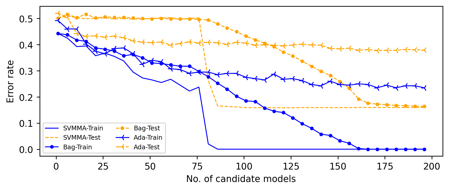
Figure 1: Learning curves under DGP1 and Scenario S1; $n$=400, $p$=1000.

We set the dimension $p$ in DGP1 and DGP2 to 1000. For Scenario S1, we set $q=5$ and omit one distinct covariate from each model at the training stage; for S2, we set $q=4$ and omit no variable. We apply the pre-screening step in Algorithm 1, set $a=0.001$ and $b=10$ for the range of $\lambda$, and $L=50$ for ordering the covariates. We choose $S_{n}$ such that the SVMMA results in the smallest risk as seen from the learning curves. For example, in Figure 1, when $S_{n}$ is in $(75,160)$, the error rates of the SVMMA method for both the training and test samples are at their lowest. We set $S_{n}=100$ but other values within the range of $(75,160)$ can also be chosen. We let the candidate models constructed for the SVMMA method be the base learners for bagging and adaboosting. This is to facilitate a fair comparison between model averaging and the two ensemble learning methods. We use a five-fold CV to calculate the model weights, and set $D=200$ and the sizes of the training and test samples to $n=100,200,300,400$ and $n_{test}=10000$ respectively.

4.3 Simulation results

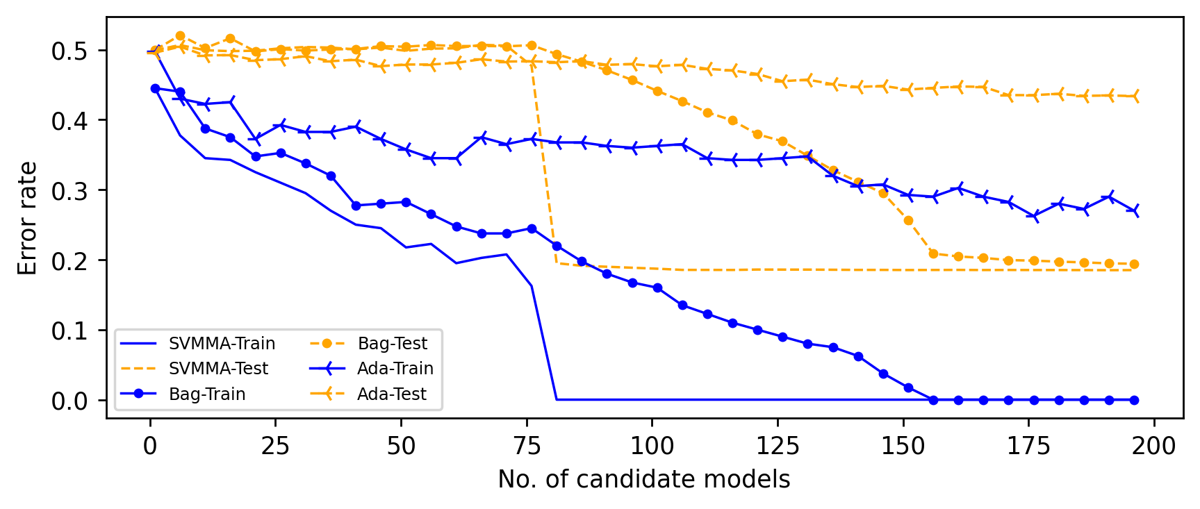
Figure 2: Learning curves under DGP2 and Scenario S1; $n$=400, $p$=1000.

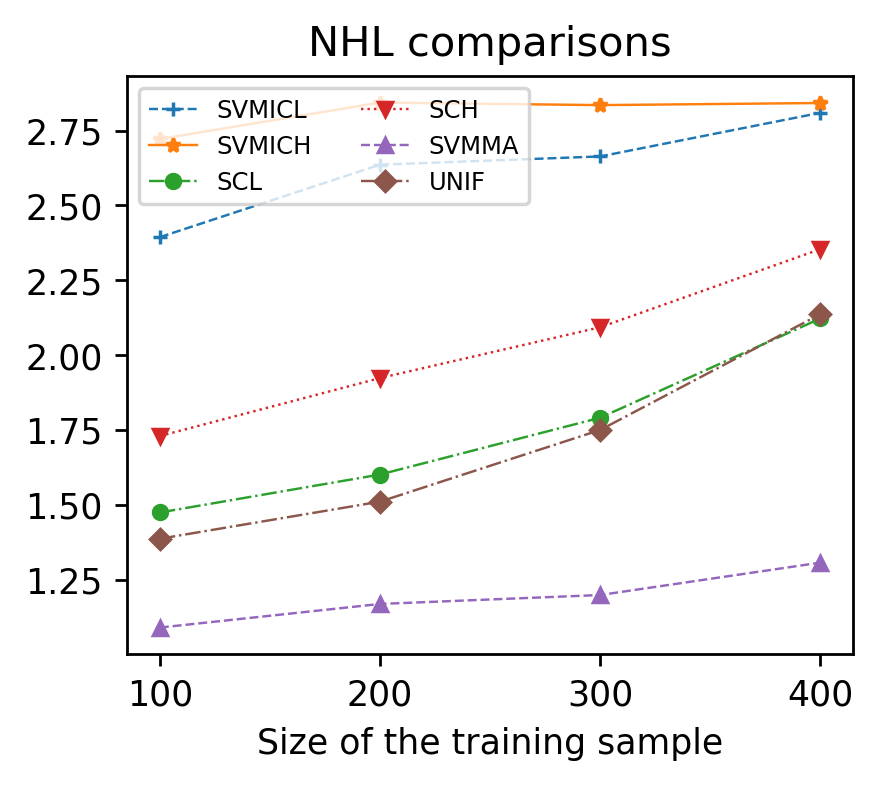
(a) DGP1

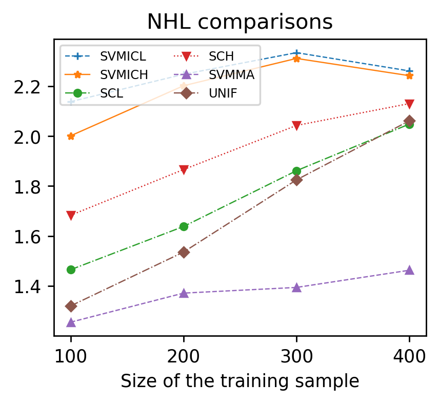
(b) DGP2

Figure 3: NHL under Scenario S1.

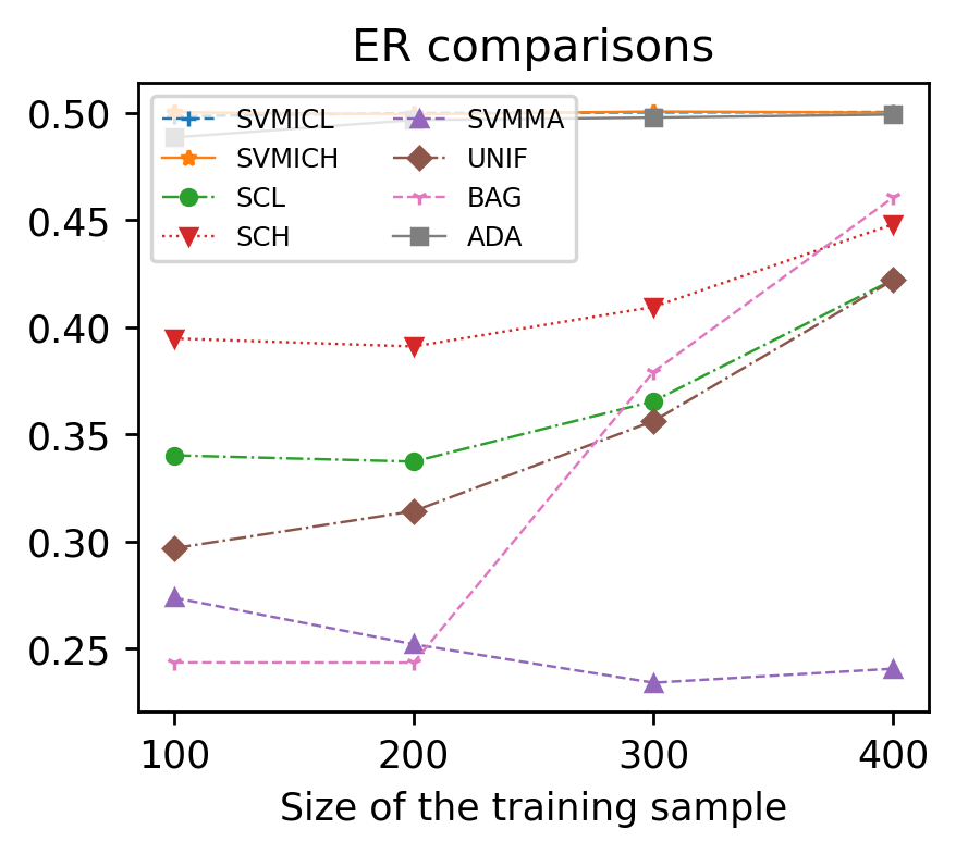
(b) DGP2

Figure 4: ER under Scenario S1.

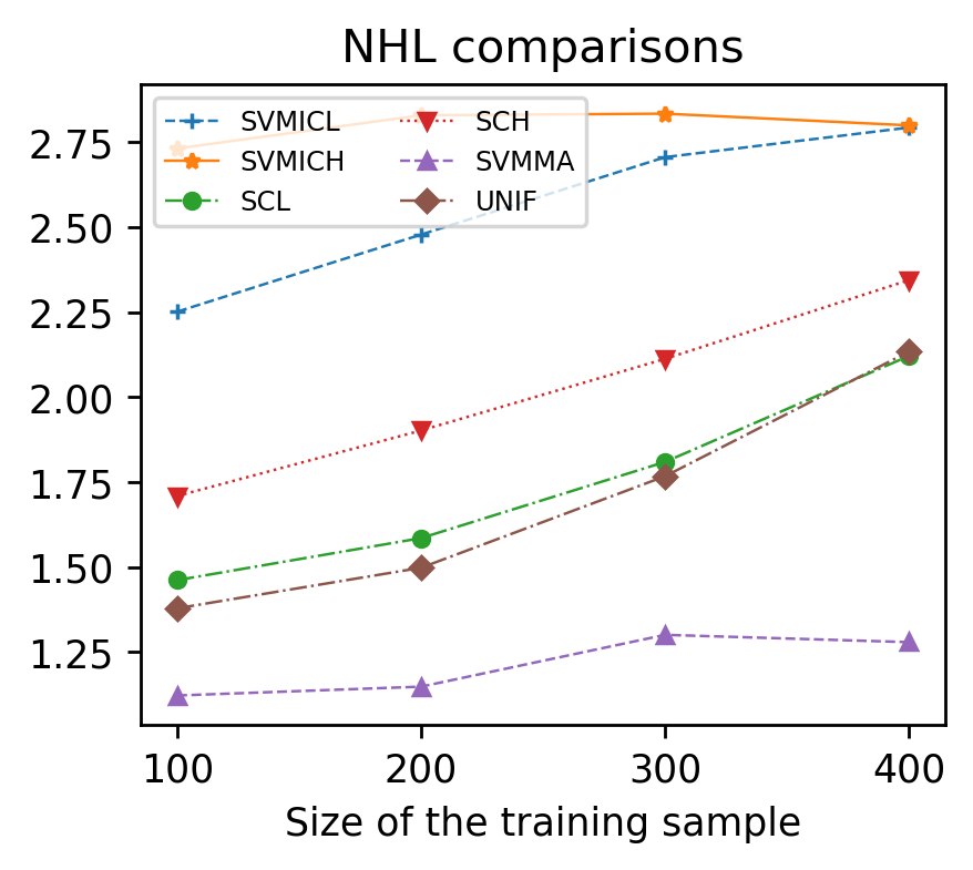
(a) DGP1

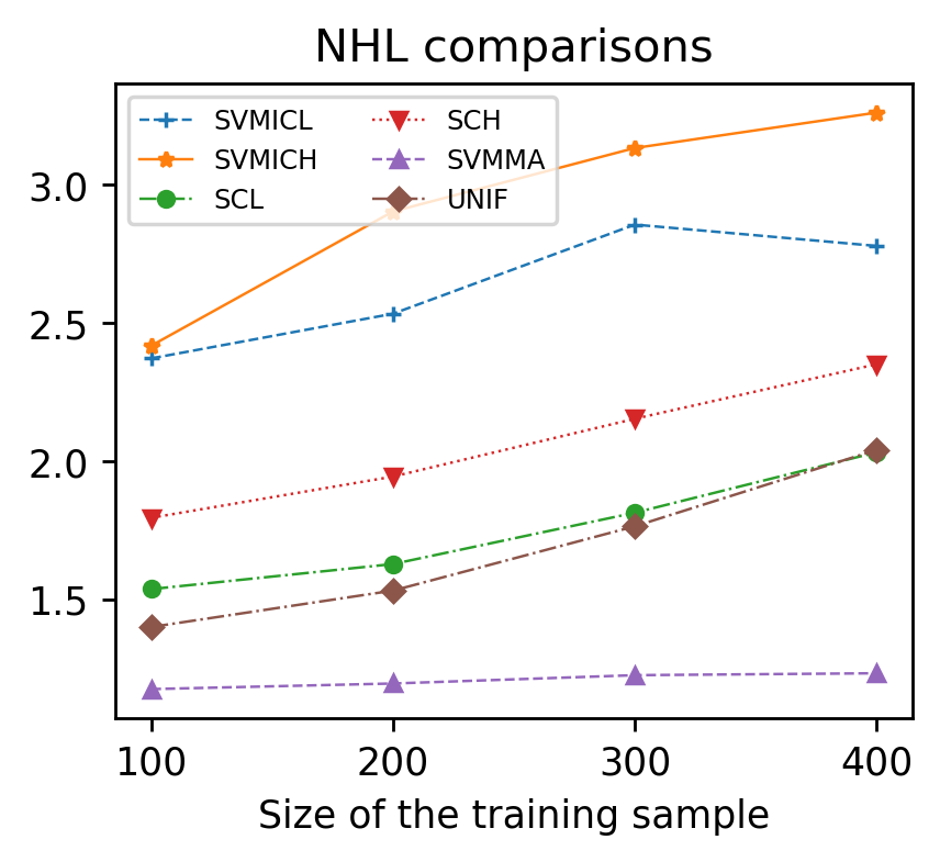
(b) DGP2

Figure 5: NHL under Scenario S2.

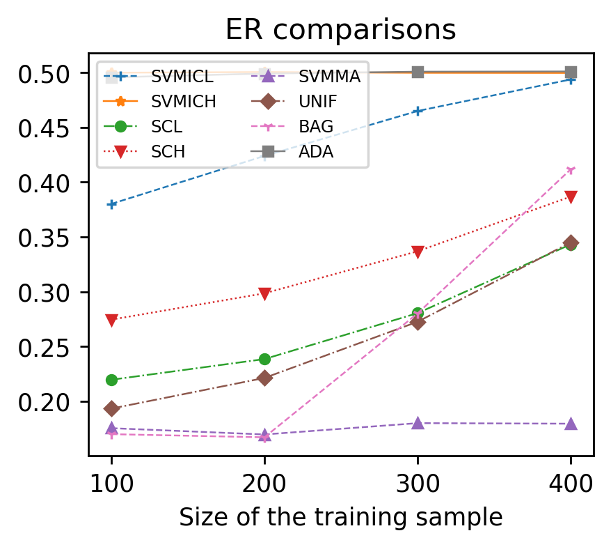
(a) DGP1

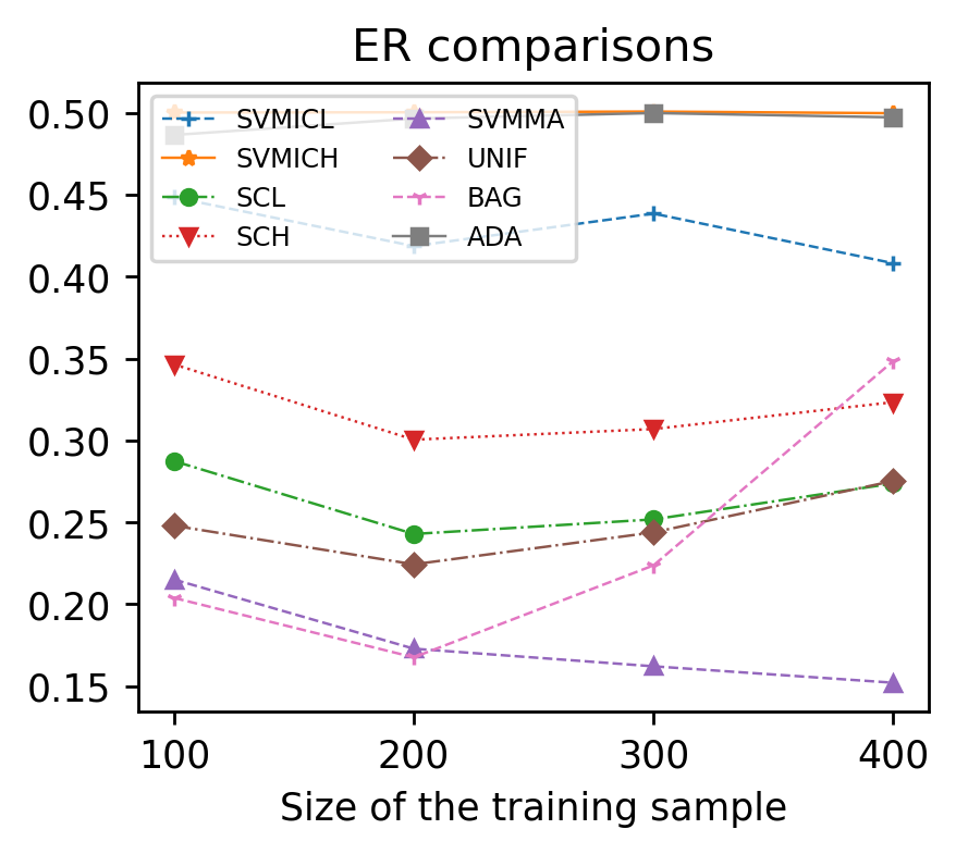
(b) DGP2

Figure 6: ER under Scenario S2.

The results are shown in Figures 1-6, where $(.)$-Train and $(.)$-Test in Figures 1-2 represent the error rates of a given method in the training and test samples respectively. Figures 1-2 show that generally speaking, the performance of SVMMA, bagging and adaboosting methods all improve as the number of base learners or candidate models increases, although in the case of adaboosting the improvement is not remarkable. For a given number of candidate models or base learners, SVMMA produces the best results in the majority of cases; while bagging is able to produce similar results to SVMMA, it can do so only at the expense of a larger number of base learners. This is a notable advantage of the proposed model averaging approach over bagging. Judging from the learning curves in 1-2, the superior SVMMA results are achieved by setting $S_{n}$ in (75, 160).

Figures 3-4 show that in terms of NHL, in all parts of the parameter space, the SVMMA approach delivers the best estimates, often by a large margin, the SCL estimator always has the edge over the SCH estimator, and both the SCL and SCH estimators dominate their corresponding model selection counterparts, the SVMICL and SVMICH estimators. Although the UNIF method is a distant second best compared to the SVMMA estimator, it is superior to the SCL estimator in terms of NHL over a large part of the parameter space. Exceptions occur when $n$ is very large, where the SCL can sometimes be slightly more accurate.

Generally speaking, the above findings carry over to comparisons in terms of ER. In all cases, adaboosting performs poorly, at a level comparable to the SVMICH estimator. On the other hand, bagging can sometimes deliver marginally better estimates than the SVMMA estimator when $n$ is small. That being said, bagging is an inferior strategy compared to most other methods when $n$ is moderate to large, while SVMMA offers more stable performance and is the preferred estimator in the majority of cases. The rather erratic performance of bagging can be explained by noting that a good bagging method relies on many independent learners (Zhou, 2012). However, in our case, every two candidate models have at least one common covariate, and as the training sample size grows, the diversity of their outcomes reduces. On the other hand, in the case of the SVMMA estimator, the weights reflect the strength of the candidate models, and better candidate models will be given higher weights, resulting in improved accuracy. It is instructive to note that a model average estimator with a weight constraint may be interpreted as a shrinkage estimator that balances between bias and variance (Jagannathan and Ma, 2003).

5 Real data examples

In this section, we apply the proposed methods to three real data sets, all obtained from the University of California at Irvine’s Machine Learning Repository. In all cases, we standardise the covariates and randomly split the data into a training subset and a test subset, containing $n$ and $n_{test}$ observations respectively. Write $N=n+n_{test}$ and $n=\lfloor g\times N\rfloor$, and let $g\in\{40\%,50\%,60\%,70\%,80\%\}$. We repeat the process of splitting the data 200 times, and calculate NHL and ER on that basis. The candidate models or base learners are generated in the same manner as in the simulation analysis. Our computation of the SVMMA weights is based on a five-fold CV.

Our first data set, labelled as “Sonar, Mines versus Rocks” (Dua and Graff, 2017), is downloadable from https://archive.ics.uci.edu/ml/datasets/Connectionist+Bench+(Sonar,+Mines+vs.+Rocks). The data contain 60 features and 208 observations. Our response variable is a binary variable that takes on 1 or 0 depending on whether the object is rock or mine. The features are signal information from sonars. More description can be found in Gorman and Sejnowski (1988). We set the number of candidate models to 20 based on the learning curve in Figure 7.

The second data set, labelled as “Ionosphere”, is downloadable from https://archive.ics.uci.edu/ml/datasets/ionosphere. The sample size is 351 with 33 features. The response is a binary variable that takes on 1 if the radar returns show evidence of some type of structure in the ionosphere, and 0 otherwise. The features are the information about electrons recorded by radars. More descriptions can be found in Sigillito et al. (1989). Judging from the behaviour of the learning curve in Figure 9, we set the number of candidate models to 30.

The third data set labelled as “LSVT Voice Rehabilitation”, is downloadable from https://archive.ics.uci.edu/ml/datasets/LSVT+Voice+Rehabilitation. The sample size is 126 with 309 features. The response is a binary variable equal to 1 if the subject is diagnosed with Parkinson’s disease, and 0 otherwise. The features are the biomedical speech signals. More description can be found in Tsanas et al. (2014). We set the number of candidate models to 30 according to the learning curve in Figure 11.

The learning abilities of model averaging and ensemble learning methods are compared in Figures 7, 9 and 11, where the $x$- and $y$-axes represent the number of candidate models and the error rates respectively. In all cases, the sizes of the training and test samples are 80% and 20% of the full sample size respectively. As is expected, for a given method, the ER associated with the training data is typically smaller than that associated with the test data. The learning ability of a method is often evaluated in terms of the stability of the ER it produces under the test sample - a method is deemed to be good if it leads to a small ER that stablises at a small value of the number of candidate models (i.e, $x$-axis). From that point of view, model averaging clearly outperforms the two ensemble learning methods, as revealed in the figures. One distinct advantage of SVMMA compared with bagging and adaboosting, is that it requires fewer base learners to achieve the same results.

Figures 8, 10 and 12 provide a comparison of the SVMMA with the SCH, SCL, SVMICH, SVMICL and UNIF methods in terms of NHL and ER in the test sample when the size of training sample varies between 40% and 80% of the total sample size. The results show that SVMMA is frequently the best performer in the pool with respect to both yardsticks. In addition, the fact that the curves of NHL of SVMMA are very close to 1, corroborates Theorem 1 because NHL is an estimate of $R_{n}(\widehat{{\bf w}})/\inf_{{\bf w}\in{\mathcal{W}}}R_{n}({\bf w})$. When NHL is near 1, it implies $R_{n}(\widehat{{\bf w}})/\inf_{{\bf w}\in{\mathcal{W}}}R_{n}({\bf w})\to 1$. Similar to the results of the simulation analysis, the SCL and SCH model averaging methods invariably deliver superior performance to their model selection counterparts, the SVMICL and SVMICH methods.

6 Concluding remarks

This paper develops a model averaging method based on cross-validation for SVM. We provided a weight choice criterion and showed that the resulting SVMMA estimator is asymptotically optimal in the sense of achieving the lowest hinge loss among all feasible models. We also developed a model screening method based on $L_{1}$ penalty. Our simulation and real data analysis shows that the proposed model average estimator performs well, compared with several other selection, averaging and ensemble learning methods. Work in progress by the authors develops optimal model averaging strategies for multi-kernel SVM models, which involve the choice of kernel as another layer of uncertainty.

(a) DGP1

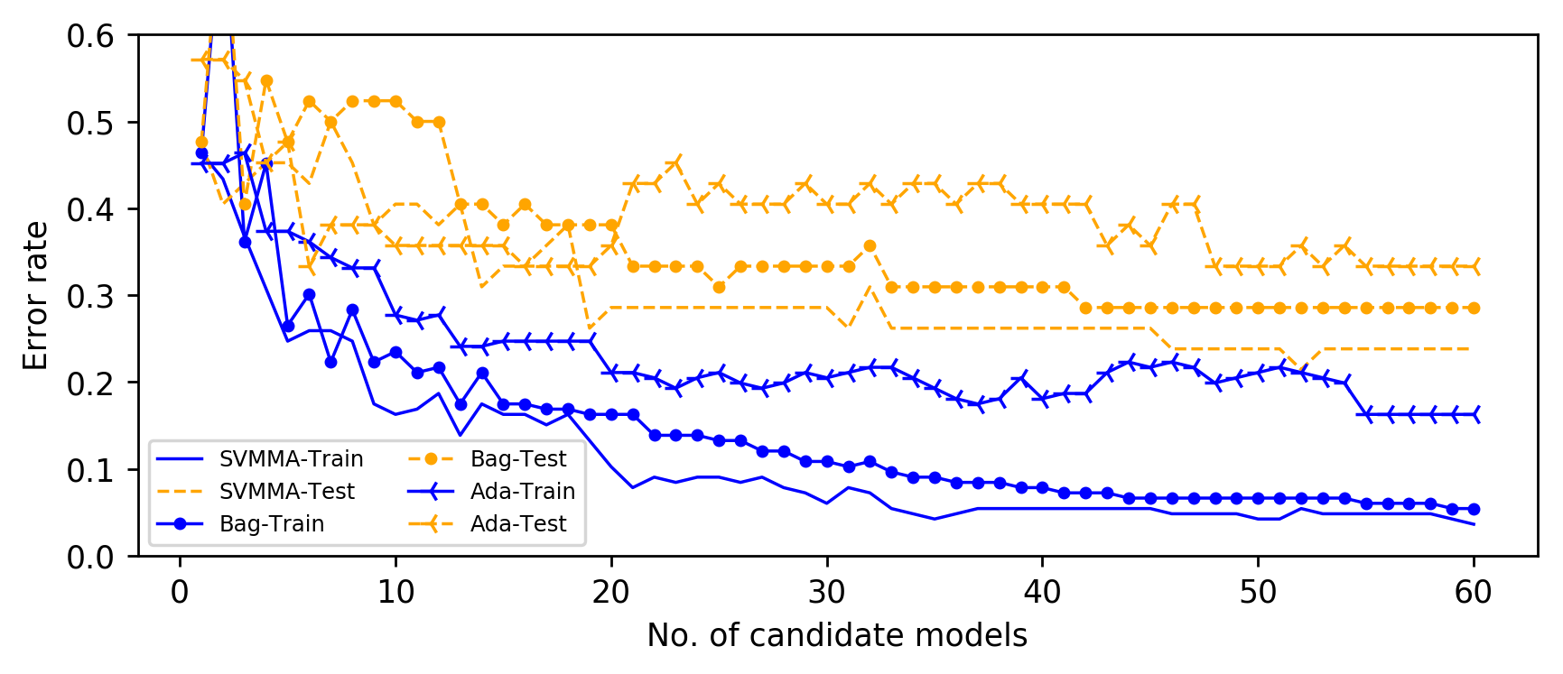
Figure 7: Learning curves for the Sonar data example; Sizes of the training and test samples are $\lfloor 80\%N\rfloor$ and $\lfloor 20\%N\rfloor$ respectively.

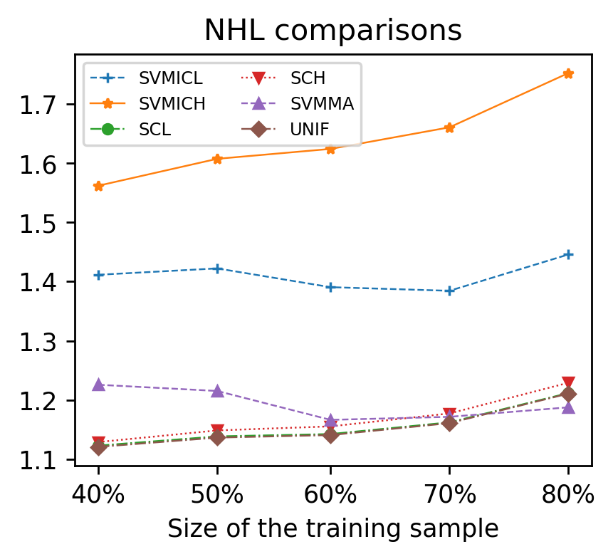
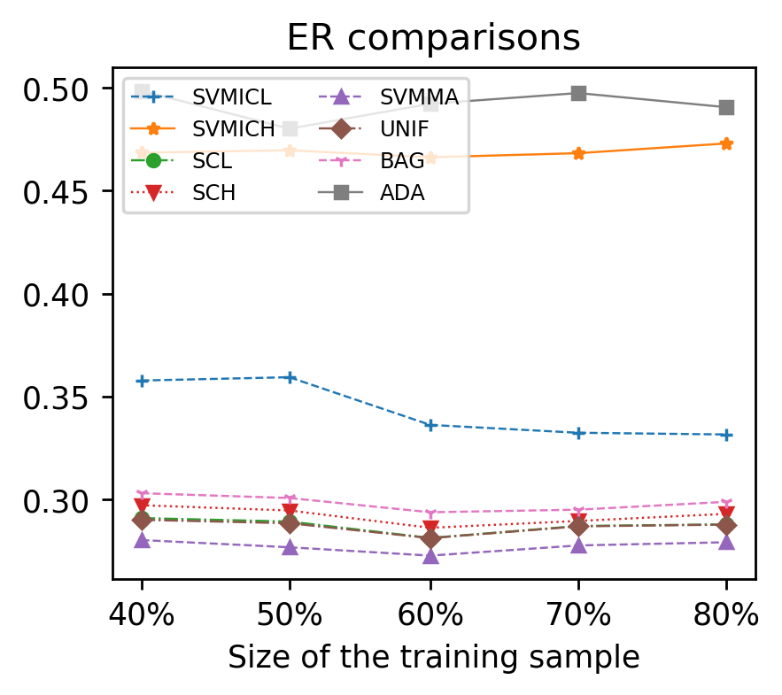
Figure 8: Comparisons for the Sonar data example.

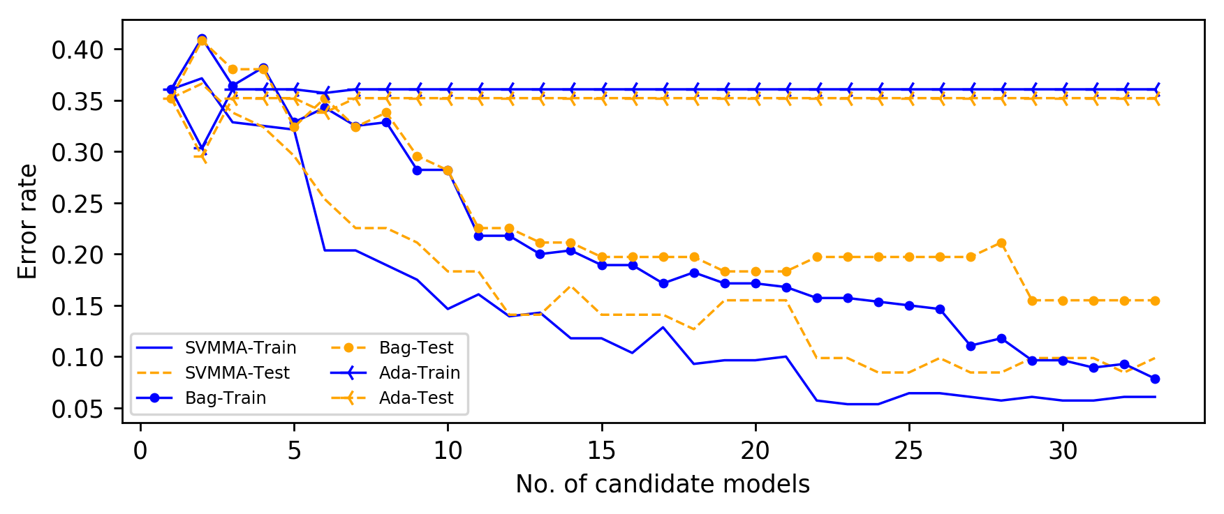
Figure 9: Learning curves for the Ionosphere data example; Sizes of the training and test samples are $\lfloor 80\%N\rfloor$ and $\lfloor 20\%N\rfloor$ respectively.

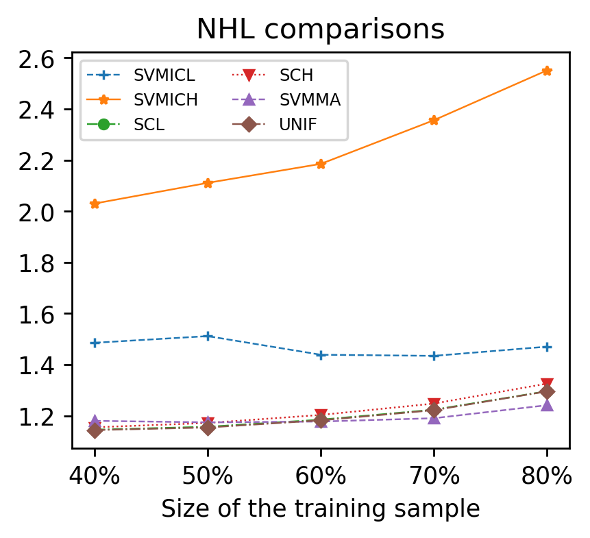
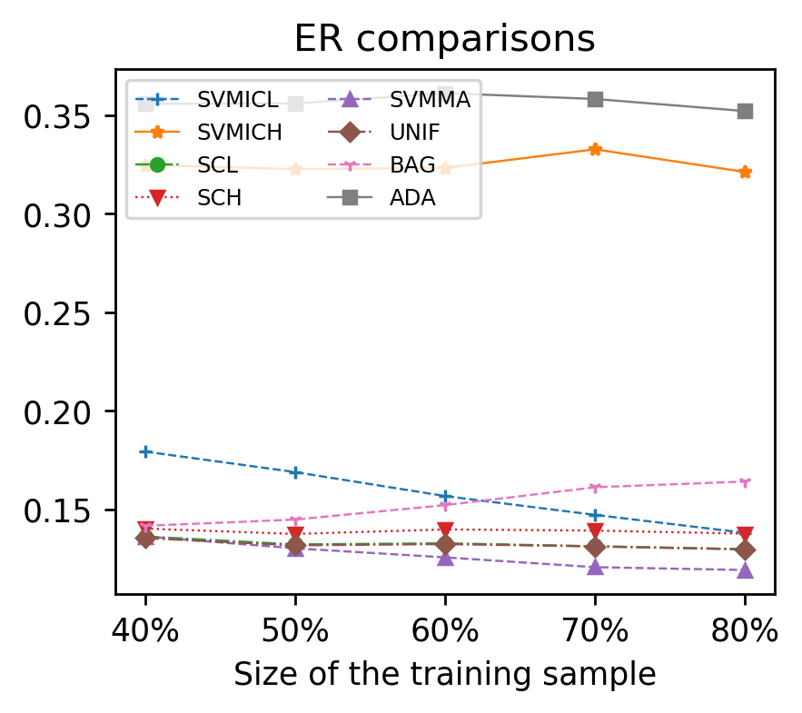
Figure 10: Comparisons for the Ionosphere data example.

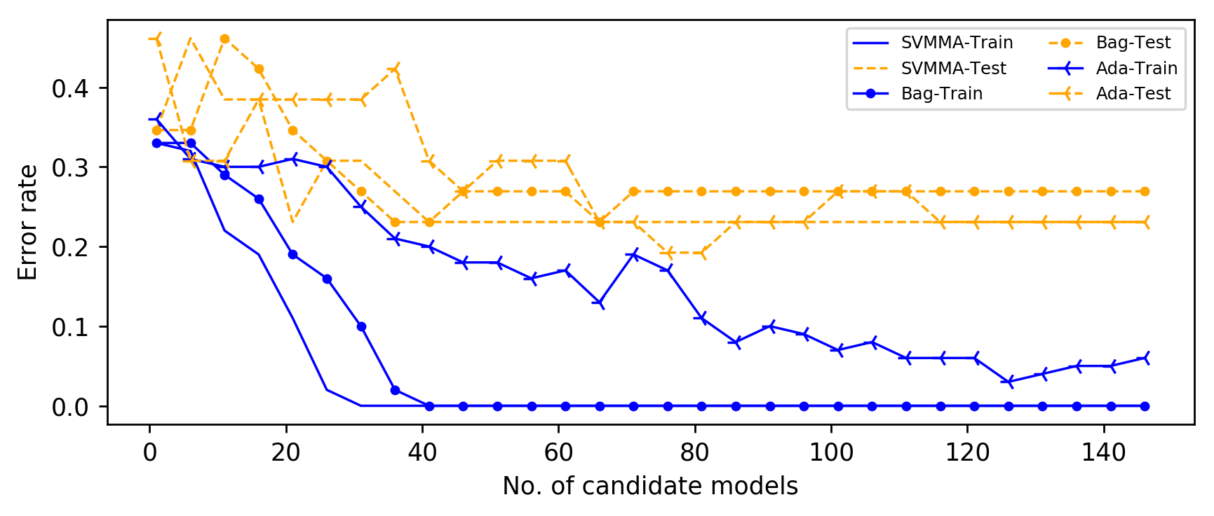
Figure 11: Learning curves for the LSVT data example; Sizes of the training and test samples are $\lfloor 80\%N\rfloor$ and $\lfloor 20\%N\rfloor$ respectively.

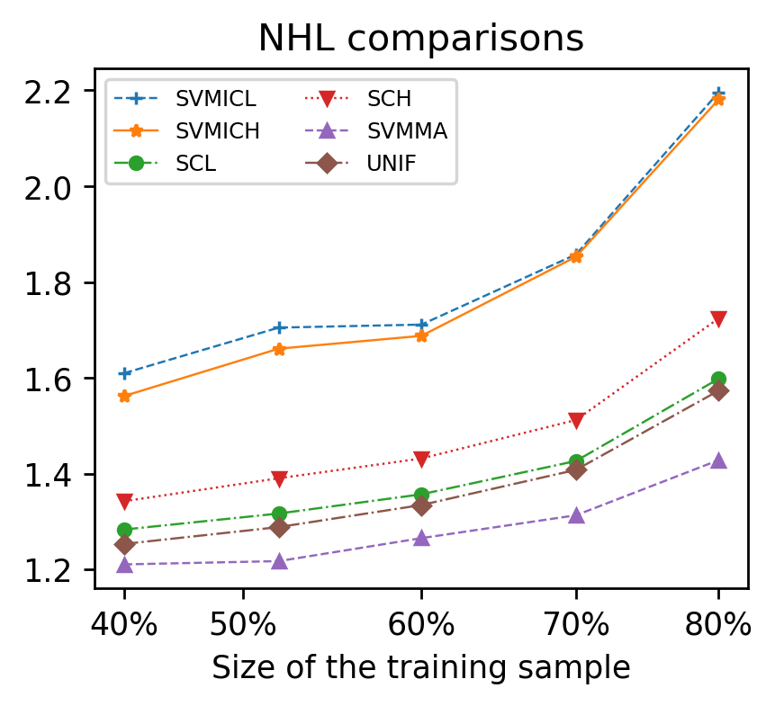
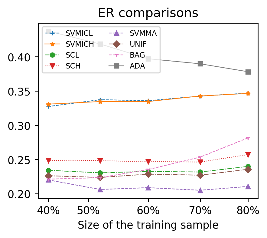
Figure 12: Comparisons for the LSVT data example.

Appendix A Appendix

This section provides the proof of Theorem 1. All limiting processes below correspond to $n\to\infty$ unless stated otherwise.

A.1 Proof of Lemma 1

Proof Part of this proof follows from Zhang et al. (2016c), but there are some differences and the conclusion is also different from that of Zhang et al. (2016c).

We will prove (9) first. Recall that $\widehat{\mbox{\boldmath${\beta}$}}_{(s)}=\arg\min_{\mbox{\boldmath${\beta}$}_{(s)}}\{n^{-1}\sum_{i=1}^{n}(1-y_{i}{\bf x}_{{(s)},i}^{\rm T}\mbox{\boldmath${\beta}$}_{(s)})+2^{-1}\lambda_{n}\|\mbox{\boldmath${\beta}$}_{(s)}^{+}\|^{2}\}$. We will show that, for any $0<\eta<1$, there exist a large constant $\triangle>0$ and an integer $N$ such that when $n>N$, we have

$$\mathrm{Pr}\left\{\min_{1\leq s\leq S_{n}}\inf_{\|{\bf u}_{(s)}\|=\triangle}\left\{l_{s}\left(\mbox{\boldmath${\beta}$}^{\ast}_{(s)}+\sqrt{n^{-1}{p_{\max}}\log({p_{\max}})}{\bf u}_{(s)}\right)-l_{s}(\mbox{\boldmath${\beta}$}^{\ast}_{(s)})\right\}>0\right\}>1-\eta,$$ (19)

where ${\bf u}_{(s)}\in\mathcal{R}^{p_{s}}$ and $l_{s}(\mbox{\boldmath${\beta}$}_{(s)})=n^{-1}\sum_{i=1}^{n}(1-y_{i}{\bf x}_{{(s)},i}^{\rm T}\mbox{\boldmath${\beta}$}_{(s)})_{+}+2^{-1}\lambda_{n}\|\mbox{\boldmath${\beta}$}_{(s)}^{+}\|^{2}$. As the hinge loss is convex, this implies that with probability $1-\eta$, $\max_{1\leq s\leq S_{n}}\|\widehat{\mbox{\boldmath${\beta}$}}_{(s)}-\mbox{\boldmath${\beta}$}^{\ast}_{(s)}\|\leq\triangle\sqrt{n^{-1}{p_{\max}}\log({p_{\max}})}$. Hence equation (9) in Lemma 1 holds.

Note that $l_{s}\left(\mbox{\boldmath${\beta}$}^{\ast}_{(s)}+\sqrt{n^{-1}{p_{\max}}\log({p_{\max}})}{\bf u}_{(s)}\right)-l_{s}\left(\mbox{\boldmath${\beta}$}^{\ast}_{(s)}\right)$ can be expressed as

$$\quad l_{s}\left(\mbox{\boldmath${\beta}$}^{\ast}_{(s)}+\sqrt{n^{-1}{p_{\max}}\log({p_{\max}})}{\bf u}_{(s)}\right)-l_{s}\left(\mbox{\boldmath${\beta}$}^{\ast}_{(s)}\right)$$

$$=n^{-1}\sum_{i=1}^{n}\left\{\left(1-y_{i}{\bf x}_{{(s)},i}^{\rm T}(\mbox{\boldmath${\beta}$}^{\ast}_{(s)}+\sqrt{n^{-1}{p_{\max}}\log({p_{\max}})}{\bf u}_{(s)})\right)_{+}-\left(1-y_{i}{\bf x}_{{(s)},i}^{\rm T}\mbox{\boldmath${\beta}$}^{\ast}_{(s)}\right)_{+}\right\}$$

$$\quad+2^{-1}\lambda_{n}\left\|\mbox{\boldmath${\beta}$}^{\ast+}_{(s)}+\sqrt{n^{-1}{p_{\max}}\log({p_{\max}})}{\bf u}_{(s)}^{+}\right\|^{2}-2^{-1}\lambda_{n}\|\mbox{\boldmath${\beta}$}^{\ast+}_{(s)}\|^{2}.$$ (20)

It is readily shown that

$$\quad\max_{1\leq s\leq S_{n}}\sup_{\|{\bf u}_{(s)}\|=\triangle}\left|\left\|\mbox{\boldmath${\beta}$}^{\ast+}_{(s)}+\sqrt{n^{-1}{p_{\max}}\log({p_{\max}})}{\bf u}_{(s)}^{+}\right\|^{2}-\left\|\mbox{\boldmath${\beta}$}^{\ast+}_{(s)}\right\|^{2}\right|$$

$$\leq\max_{1\leq s\leq S_{n}}\sup_{\|{\bf u}_{(s)}\|=\triangle}\left(\left\|\mbox{\boldmath${\beta}$}^{\ast+}_{(s)}+\sqrt{n^{-1}{p_{\max}}\log({p_{\max}})}{\bf u}_{(s)}^{+}\right\|+\left\|\mbox{\boldmath${\beta}$}^{\ast+}_{(s)}\right\|\right)\left\|\sqrt{n^{-1}{p_{\max}}\log({p_{\max}})}{\bf u}_{(s)}^{+}\right\|$$

$$\leq 2\triangle C_{2}{p_{\max}}\sqrt{n^{-1}\log({p_{\max}})}+\triangle n^{-1}{p_{\max}}\log({p_{\max}})$$

$$=O(\triangle{p_{\max}}\sqrt{n^{-1}\log({p_{\max}})}),$$ (21)

where the last inequality is obtained from Condition 3. Hence the order of difference of penalty terms in (20) is $O(\triangle\lambda_{n}{p_{\max}}\sqrt{n^{-1}\log({p_{\max}})})$.

Denote

$$g_{s,i}({\bf u}_{(s)}) =\left(1-y_{i}{\bf x}_{{(s)},i}^{\rm T}(\mbox{\boldmath${\beta}$}^{\ast}_{(s)}+\sqrt{n^{-1}{p_{\max}}\log({p_{\max}})}{\bf u}_{(s)})\right)_{+}-\left(1-y_{i}{\bf x}_{{(s)},i}^{\rm T}\mbox{\boldmath${\beta}$}^{\ast}_{(s)}\right)_{+}$$

$$\quad+\sqrt{n^{-1}{p_{\max}}\log({p_{\max}})}y_{i}{\bf x}_{{(s)},i}^{\rm T}{\bf u}_{(s)}\mathbf{1}\left(1-y_{i}{\bf x}_{{(s)},i}^{\rm T}\mbox{\boldmath${\beta}$}^{\ast}_{(s)}\geq 0\right)$$

$$\quad-\mathbb{E}\left[\left(1-y_{i}{\bf x}_{{(s)},i}^{\rm T}(\mbox{\boldmath${\beta}$}^{\ast}_{(s)}+\sqrt{n^{-1}{p_{\max}}\log({p_{\max}})}{\bf u}_{(s)})\right)_{+}\right]+\mathbb{E}\left[\left(1-y_{i}{\bf x}_{{(s)},i}^{\rm T}\mbox{\boldmath${\beta}$}^{\ast}_{(s)}\right)_{+}\right].$$

It can be verified that $\mathbb{E}[g_{{(s)},i}({\bf u})]=0$, $s=1,2,...,S_{n}$ by the definition of $\mbox{\boldmath${\beta}$}^{\ast}_{(s)}$ and $\mathbf{J}_{(s)}(\mbox{\boldmath${\beta}$}^{\ast}_{(s)})=0$. Note that (20) can be further decomposed as

$$n^{-1}\sum_{i=1}^{n}\left\{\left(1-y_{i}{\bf x}_{{(s)},i}^{\rm T}(\mbox{\boldmath${\beta}$}^{\ast}_{(s)}+\sqrt{n^{-1}{p_{\max}}\log({p_{\max}})}{\bf u}_{(s)})\right)_{+}-\left(1-y_{i}{\bf x}_{{(s)},i}^{\rm T}\mbox{\boldmath${\beta}$}^{\ast}_{(s)}\right)_{+}\right\}=n^{-1}(A_{s,n}+B_{s,n}),$$

where

$$A_{s,n}=\sum_{i=1}^{n}g_{s,i}({\bf u}_{(s)})$$

and

$$B_{s,n} =\sum_{i=1}^{n}\Big{[}-\sqrt{n^{-1}{p_{\max}}\log({p_{\max}})}y_{i}{\bf x}_{{(s)},i}^{\rm T}{\bf u}_{(s)}\mathbf{1}\left(1-y_{i}{\bf x}_{{(s)},i}^{\rm T}\mbox{\boldmath${\beta}$}^{\ast}_{(s)}\geq 0\right)$$

$$\quad+\mathbb{E}\left\{\left(1-y_{i}{\bf x}_{{(s)},i}^{\rm T}(\mbox{\boldmath${\beta}$}^{\ast}_{(s)}+\sqrt{n^{-1}{p_{\max}}\log({p_{\max}})}{\bf u}_{(s)})\right)_{+}\right\}-\mathbb{E}\left\{\left(1-y_{i}{\bf x}_{{(s)},i}^{\rm T}\mbox{\boldmath${\beta}$}^{\ast}_{(s)}\right)_{+}\right\}\Big{]}.$$ (22)

The remainder of the proof consists of three steps. In Step 1, we demonstrate that

$$\max_{1\leq s\leq S_{n}}\sup_{\|{\bf u}_{(s)}\|=\triangle}|A_{s,n}|=\triangle^{3/2}{p_{\max}}o_{p}(1).$$ (23)

In Step 2, it is shown that $\min_{1\leq s\leq S_{n}}\inf_{\|{\bf u}_{(s)}\|=\triangle}B_{s,n}$ dominates the terms of order $\triangle^{3/2}{p_{\max}}o_{p}(1)$ and is larger than zero. In Step 3, we use the results from the previous steps to prove (19).

Step 1: We use the covering number introduced by van der Vaart and Wellner (1996) to prove the uniform rate in (23). It suffices to show, for any $\epsilon>0$, that

$$\mathrm{Pr}\left(\max_{1\leq s\leq S_{n}}\sup_{\|{\bf u}_{(s)}\|=\triangle}p_{s}^{-1}\left|\sum_{i=1}^{n}g_{s,i}({\bf u}_{(s)})\right|>\triangle^{3/2}\epsilon\right)\to 0.$$ (24)

Note that the hinge loss satisfies the Lipschitz condition and $\max_{1\leq i\leq n}\|{\bf x}_{{(s)},i}\|\leq C_{1}\sqrt{p_{s}}$, $\max_{1\leq i\leq n}\mathbb{E}\|{\bf x}_{{(s)},i}\|\leq C_{1}\sqrt{p_{s}}$ from Condition 2. It is readily shown that

$$|g_{s,i}({\bf u}_{(s)})| \leq 3\triangle\sqrt{n^{-1}{p_{\max}}\log({p_{\max}})}\max\left\{\max_{1\leq i\leq n}\|{\bf x}_{{(s)},i}\|,\max_{1\leq i\leq n}\mathbb{E}\|{\bf x}_{{(s)},i}\|\right\}$$

$$\leq 3C_{1}\triangle{p_{\max}}\sqrt{n^{-1}\log({p_{\max}})}$$ (25)

and thus $\max_{1\leq s\leq S_{n}}\sup_{\|{\bf u}_{(s)}\|=\triangle}p_{s}^{-1}|g_{s,i}({\bf u}_{(s)})|=o(1)$ by Condition 6. By Lemma 2.5 of van de Geer (2000), the ball $\{{\bf u}_{(s)}:\|{\bf u}_{(s)}\|\leq\triangle\}$ in $\mathcal{R}^{p_{s}+1}$ can be covered by $N_{s}$ balls with radius $\zeta_{s}$, where $N_{s}\leq\{(4\triangle+\zeta_{s})/\zeta_{s}\}^{p_{s}+1}$. Denote ${\bf u}_{(s)}^{1},..,{\bf u}_{(s)}^{N}$ as the centers of the $N_{s}$ balls, let $\zeta_{s}=(nM_{1})^{-1}p_{s}$ (for some large constant $M_{1}>0$ ) and denote $\mathcal{U}_{s}^{k}=\{{\bf u}_{(s)}:\|{\bf u}_{(s)}-{\bf u}_{(s)}^{k}\|\leq\zeta_{s}\&\|{\bf u}_{(s)}\|=\triangle\}$. For any $\epsilon>0$, we have

$$\quad\max_{1\leq s\leq S_{n}}\max_{1\leq k\leq N_{s}}\sup_{{\bf u}_{(s)}\in\mathcal{U}_{s}^{(k)}}p_{s}^{-1}\left|\sum_{i=1}^{n}g_{s,i}({\bf u}_{(s)})-\sum_{i=1}^{n}g_{s,i}({\bf u}_{(s)}^{k})\right|$$

$$\leq\max_{1\leq s\leq S_{n}}\max_{1\leq k\leq N_{s}}\sup_{{\bf u}_{(s)}\in\mathcal{U}_{s}^{k}}p_{s}^{-1}\sum_{i=1}^{n}\left|g_{s,i}({\bf u}_{(s)})-g_{s,i}({\bf u}_{(s)}^{k})\right|$$

$$\leq\max_{1\leq s\leq S_{n}}\max_{1\leq k\leq N_{s}}\sup_{{\bf u}_{(s)}\in\mathcal{U}_{s}^{k}}np_{s}^{-1}\Big{\{}2\sqrt{n^{-1}{p_{\max}}\log({p_{\max}})}\|{\bf x}_{{(s)},i}\|\|{\bf u}_{(s)}-{\bf u}_{(s)}^{k}\|$$

$$\quad+\sqrt{n^{-1}{p_{\max}}\log({p_{\max}})}\|{\bf u}_{(s)}-{\bf u}_{(s)}^{k}\|\mathbb{E}\|{\bf x}_{{(s)},i}\|\Big{\}}$$

$$\leq\max_{1\leq s\leq S_{n}}3\triangle np_{s}^{-1}\sqrt{n^{-1}{p_{\max}}\log({p_{\max}})}\max\left\{\max_{1\leq i\leq n}\|{\bf x}_{{(s)},i}\|,\max_{1\leq i\leq n}\mathbb{E}\|{\bf x}_{{(s)},i}\|\right\}\zeta_{s}$$

$$\leq 3C_{1}M_{1}^{-1}\triangle{p_{\max}}\sqrt{n^{-1}\log({p_{\max}})}$$

$$=o(\triangle^{3/2}p_{\min}\epsilon/2),$$ (26)

where the last inequality arises from Condition 6. From (26), it can be shown that

$$\mathrm{Pr}\left(\max_{1\leq s\leq S_{n}}\sup_{\|{\bf u}_{(s)}\|=\triangle}p_{s}^{-1}\left|\sum_{i=1}^{n}g_{s,i}({\bf u}_{(s)})\right|>\triangle^{3/2}\epsilon\right)$$

$$\leq\mathrm{Pr}\Bigg{(}\max_{1\leq s\leq S_{n}}\max_{1\leq k\leq N_{s}}\sup_{{\bf u}_{(s)}\in\mathcal{U}_{s}^{(k)}}p_{s}^{-1}\left|\sum_{i=1}^{n}g_{s,i}({\bf u}_{(s)})-\sum_{i=1}^{n}g_{s,i}({\bf u}_{(s)}^{k})\right|$$

$$\quad+\max_{1\leq s\leq S_{n}}\max_{1\leq k\leq N_{s}}p_{s}^{-1}\left|\sum_{i=1}^{n}g_{s,i}({\bf u}_{(s)}^{k})\right|>\triangle^{3/2}\epsilon\Bigg{)}$$

$$\leq\mathrm{Pr}\Bigg{(}\max_{1\leq s\leq S_{n}}\max_{1\leq k\leq N_{s}}\sup_{{\bf u}_{(s)}\in\mathcal{U}_{s}^{(k)}}\left|\sum_{i=1}^{n}g_{s,i}({\bf u}_{(s)})-\sum_{i=1}^{n}g_{s,i}({\bf u}_{(s)}^{k})\right|>\triangle^{3/2}p_{\min}\epsilon/2\Bigg{)}$$

$$\quad+\sum_{s=1}^{S_{n}}\sum_{k=1}^{N_{s}}\mathrm{Pr}\left(\left|\sum_{i=1}^{n}g_{s,i}({\bf u}_{(s)}^{k})\right|>\triangle^{3/2}p_{s}\epsilon/2\right)$$

$$=\sum_{s=1}^{S_{n}}\sum_{k=1}^{N_{s}}\mathrm{Pr}\left(\left|\sum_{i=1}^{n}g_{s,i}({\bf u}_{(s)}^{k})\right|>\triangle^{3/2}p_{s}\epsilon/2\right)+o(1)$$ (27)

and $\sum_{i=1}^{n}g_{s,i}({\bf u}_{(s)}^{(k)})$ is the sum of independent zero-mean random variables.

By the bounded conditional density, under Conditions 1 and 4, recognising that
$\max_{1\leq i\leq n}\|{\bf x}_{{(s)},i}\|\leq C_{1}\sqrt{p_{s}}$, we have

$$\quad\mathrm{Pr}\left(|1-y_{i}{\bf x}_{{(s)},i}^{\rm T}\mbox{\boldmath${\beta}$}^{\ast}_{(s)}|\leq\sqrt{n^{-1}{p_{\max}}\log({p_{\max}})}\max_{1\leq i\leq n}\|{\bf x}_{{(s)},i}\|\triangle\right)$$

$$=\mathrm{Pr}\Big{(}\pm 1-\sqrt{n^{-1}{p_{\max}}\log({p_{\max}})}\max_{1\leq i\leq n}\|{\bf x}_{{(s)},i}\|\triangle\leq{\bf x}_{{(s)},i}^{\rm T}\mbox{\boldmath${\beta}$}^{\ast}_{(s)}\leq$$

$$\quad\sqrt{n^{-1}{p_{\max}}\log({p_{\max}})}\max_{1\leq i\leq n}\|{\bf x}_{{(s)},i}\|\triangle\pm 1\Big{|}y_{i}=\pm 1\Big{)}$$

$$\leq 2C_{3}\sqrt{n^{-1}{p_{\max}}\log({p_{\max}})}\max_{1\leq i\leq n}\|{\bf x}_{{(s)},i}\|\triangle$$

$$\leq 2\triangle C_{1}C_{3}\sqrt{n^{-1}p_{s}{p_{\max}}\log({p_{\max}})}.$$ (28)

Note that when $1-y_{i}{\bf x}_{{(s)},i}^{\rm T}\mbox{\boldmath${\beta}$}^{\ast}_{(s)}<\sqrt{n^{-1}{p_{\max}}\log({p_{\max}})}y_{i}{\bf x}_{{(s)},i}^{\rm T}{\bf u}_{(s)}$ and $\sqrt{n^{-1}{p_{\max}}\log({p_{\max}})}\\ y_{i}{\bf x}_{{(s)},i}^{\rm T}{\bf u}_{(s)}<0$, or when $1-y_{i}{\bf x}_{{(s)},i}^{\rm T}\mbox{\boldmath${\beta}$}^{\ast}_{(s)}>\sqrt{n^{-1}{p_{\max}}\log({p_{\max}})}y_{i}{\bf x}_{{(s)},i}^{\rm T}{\bf u}_{(s)}$ and $\sqrt{n^{-1}{p_{\max}}\log({p_{\max}})}\\ y_{i}{\bf x}_{{(s)},i}^{\rm T}{\bf u}_{(s)}>0$,

$$\left(1-y_{i}{\bf x}_{{(s)},i}^{\rm T}(\mbox{\boldmath${\beta}$}^{\ast}_{(s)}+\sqrt{n^{-1}{p_{\max}}\log({p_{\max}})}{\bf u}_{(s)})\right)_{+}-(1-y_{i}{\bf x}_{{(s)},i}^{\rm T}\mbox{\boldmath${\beta}$}^{\ast}_{(s)})_{+}$$

$$\quad+\sqrt{n^{-1}{p_{\max}}\log({p_{\max}})}y_{i}{\bf x}_{{(s)},i}^{\rm T}{\bf u}_{(s)}\mathbf{1}(1-y_{i}{\bf x}_{{(s)},i}^{\rm T}\mbox{\boldmath${\beta}$}^{\ast}_{(s)}\geq 0)=0.$$ (29)

Furthermore, equation (29) holds when $|1-y_{i}{\bf x}_{{(s)},i}^{\rm T}\mbox{\boldmath${\beta}$}^{\ast}_{(s)}|>\sqrt{n^{-1}{p_{\max}}\log({p_{\max}})}\max_{1\leq i\leq n}\|{\bf x}_{{(s)},i}\|\triangle$ as $\sqrt{n^{-1}{p_{\max}}\log({p_{\max}})}\max_{1\leq i\leq n}\|{\bf x}_{{(s)},i}\|\triangle>\left|\sqrt{n^{-1}{p_{\max}}\log({p_{\max}})}y_{i}{\bf x}_{{(s)},i}^{\rm T}{\bf u}_{(s)}\right|$. Hence we can write

$$\quad\sum_{i=1}^{n}\mathbb{E}\{g^{2}_{s,i}({\bf u}_{(s)}^{k})\}$$ (30)

$$\leq\sum_{i=1}^{n}\mathbb{E}\Bigg{[}\Bigg{\{}\Big{|}\left(1-y_{i}{\bf x}_{{(s)},i}^{\rm T}(\mbox{\boldmath${\beta}$}^{\ast}_{(s)}+\sqrt{n^{-1}{p_{\max}}\log({p_{\max}})}{\bf u}_{(s)}^{k})\right)_{+}-\left(1-y_{i}{\bf x}_{{(s)},i}^{\rm T}\mbox{\boldmath${\beta}$}^{\ast}_{(s)}\right)_{+}\Big{|}$$

$$\quad+\Big{|}\sqrt{n^{-1}{p_{\max}}\log({p_{\max}})}y_{i}{\bf x}_{{(s)},i}^{\rm T}{\bf u}_{(s)}^{k}\Big{|}\Bigg{\}}^{2}\mathbf{1}\Big{(}|1-y_{i}{\bf x}_{{(s)},i}^{\rm T}\mbox{\boldmath${\beta}$}^{\ast}_{(s)}|\leq\sqrt{n^{-1}{p_{\max}}\log({p_{\max}})}$$

$$\quad\times\max_{1\leq i\leq n}\|{\bf x}_{{(s)},i}\|\triangle\Big{)}\Bigg{]}$$

$$\leq\sum_{i=1}^{n}\mathbb{E}\Bigg{\{}\left(2\sqrt{n^{-1}{p_{\max}}\log({p_{\max}})}{\bf x}_{{(s)},i}^{\rm T}{\bf u}_{(s)}^{k}\right)^{2}\mathbf{1}\Big{(}|1-y_{i}{\bf x}_{{(s)},i}^{\rm T}\mbox{\boldmath${\beta}$}^{\ast}_{(s)}|\leq\sqrt{n^{-1}{p_{\max}}\log({p_{\max}})}$$

$$\quad\times\max_{1\leq i\leq n}\|{\bf x}_{{(s)},i}\|\triangle\Big{)}\Bigg{\}}$$

$$\leq\left(2\sqrt{n^{-1}{p_{\max}}\log({p_{\max}})}\max_{1\leq i\leq n}\|{\bf x}_{{(s)},i}\|\triangle\right)^{2}\sum_{i=1}^{n}\mathbb{E}\Big{(}|1-y_{i}{\bf x}_{{(s)},i}^{\rm T}\mbox{\boldmath${\beta}$}^{\ast}_{(s)}|\leq\sqrt{n^{-1}{p_{\max}}\log({p_{\max}})}$$

$$\quad\times\max_{1\leq i\leq n}\|{\bf x}_{{(s)},i}\|\triangle\Big{)}$$

$$\leq 4C_{1}^{2}\triangle^{2}n^{-1}p_{s}{p_{\max}}\log({p_{\max}})\sum_{i=1}^{n}\mathbb{E}\Big{(}|1-y_{i}{\bf x}_{{(s)},i}^{\rm T}\mbox{\boldmath${\beta}$}^{\ast}_{(s)}|\leq\sqrt{n^{-1}{p_{\max}}\log({p_{\max}})}\max_{1\leq i\leq n}\|{\bf x}_{{(s)},i}\|\triangle\Big{)}$$

$$\leq 4C_{1}^{2}\triangle^{2}n^{-1}p_{s}{p_{\max}}\log({p_{\max}})\times 2n\triangle C_{1}C_{3}\sqrt{n^{-1}p_{s}{p_{\max}}\log({p_{\max}})}$$

$$=8\triangle^{3}C_{1}^{3}C_{3}n^{-1/2}p_{s}^{3/2}p^{3/2}_{\max}\log^{3/2}({p_{\max}}),$$ (31)

where the second-to-last inequality arises from $\max_{1\leq i\leq n}\|{\bf x}_{{(s)},i}\|\leq C_{1}\sqrt{p_{s}}$ and the last inequality is from (28). Finally, by Bernstein’s inequality and recognising (25) and (31), we can write

$$\quad\sum_{s=1}^{S_{n}}\sum_{k=1}^{N_{s}}\mathrm{Pr}\left(\left|\sum_{i=1}^{n}g_{s,i}({\bf u}^{k})\right|>\triangle^{3/2}p_{s}\epsilon/2\right)$$

$$\leq\sum_{s=1}^{S_{n}}\sum_{k=1}^{N_{s}}2\exp\left(-\frac{\triangle^{3}p_{s}^{2}\epsilon^{2}/4}{\sum_{i=1}^{n}\mathbb{E}\{g_{s,i}^{2}({\bf u}^{k})\}+3\triangle^{5/2}C_{1}p_{s}{p_{\max}}\sqrt{n^{-1}\log({p_{\max}})}\epsilon/2}\right)$$

$$\leq\sum_{s=1}^{S_{n}}\left(\frac{4\triangle+(nM_{1})^{-1}p_{s}}{(nM_{1})^{-1}p_{s}}\right)^{p_{s}+1}$$

$$\quad\times\exp\left(-\frac{\triangle^{3}p_{s}^{2}\epsilon^{2}/4}{8\triangle^{3}C_{1}^{3}C_{3}n^{-1/2}p_{s}^{3/2}p^{3/2}_{\max}\log^{3/2}({p_{\max}})+3\triangle^{5/2}C_{1}p_{s}{p_{\max}}\sqrt{n^{-1}\log({p_{\max}})}\epsilon/2}\right)$$

$$\leq S_{n}\left(\frac{4\triangle M_{1}n}{p_{\min}}+1\right)^{{p_{\max}}+1}\exp\left(-\frac{\triangle^{3}p_{\min}^{1/2}\epsilon^{2}/4}{16\triangle^{3}C_{1}^{3}C_{3}n^{-1/2}p^{3/2}_{\max}\log^{3/2}({p_{\max}})}\right)$$

$$=O(1)\exp\left\{\log(S_{n})+({p_{\max}}+1)\log(4\triangle nM_{1}p^{-1}_{\min}+1)-64^{-1}C_{1}^{-3}C_{3}^{-1}\epsilon^{2}n^{1/2}p_{\min}^{1/2}p^{-3/2}_{\max}\log^{-3/2}({p_{\max}})\right\}$$

$$=o(1),$$ (32)

where the last equality is due to Condition 6 and $S_{n}=O\{\exp(n^{\tau})\}$ for $\tau\in(0,1/2-3\kappa/2)$. The proof of (24) is complete by combining (27) and (32).

Step 2: Let us rewrite $B_{s,n}$ as $B_{s,n}\equiv B_{s,n1}+B_{s,n2}$, where

$$B_{s,n1} =-\sum_{i=1}^{n}\sqrt{n^{-1}{p_{\max}}\log({p_{\max}})}y_{i}{\bf x}_{{(s)},i}^{\rm T}{\bf u}_{s}\mathbf{1}\left(1-y_{i}{\bf x}_{{(s)},i}^{\rm T}\mbox{\boldmath${\beta}$}^{\ast}_{(s)}\geq 0\right),$$

and

$$B_{s,n2} =\mathbb{E}\left\{\left(1-y_{i}{\bf x}_{{(s)},i}^{\rm T}(\mbox{\boldmath${\beta}$}^{\ast}_{(s)}+\sqrt{n^{-1}{p_{\max}}\log({p_{\max}})}{\bf u}_{(s)})\right)_{+}\right\}-\mathbb{E}\left\{\left(1-y_{i}{\bf x}_{{(s)},i}^{\rm T}\mbox{\boldmath${\beta}$}^{\ast}_{(s)}\right)_{+}\right\}.$$

To analyse $B_{s,n1}$, we observe that

$$\quad\left|\sum_{i=1}^{n}y_{i}{\bf x}_{{(s)},i}^{\rm T}{\bf u}_{(s)}\mathbf{1}\left(1-y_{i}{\bf x}_{{(s)},i}^{\rm T}\mbox{\boldmath${\beta}$}^{\ast}_{(s)}\geq 0\right)\right|$$

$$=\left|\sum_{j=0}^{p_{s}}\sum_{i=1}^{n}y_{i}{\bf x}_{{(s)},ij}u_{{(s)},j}\mathbf{1}\left(1-y_{i}{\bf x}_{{(s)},i}^{\rm T}\mbox{\boldmath${\beta}$}^{\ast}_{(s)}\geq 0\right)\right|$$

$$\leq\sum_{j=0}^{p_{s}}|u_{{(s)},j}|\max_{0\leq j\leq p_{s}}\left|\sum_{i=1}^{n}y_{i}x_{{(s)},ij}\mathbf{1}\left(1-y_{i}{\bf x}_{{(s)},i}^{\rm T}\mbox{\boldmath${\beta}$}^{\ast}_{(s)}\geq 0\right)\right|$$

$$\leq\sqrt{\sum_{j=0}^{p_{s}}u_{{(s)},j}^{2}}\sqrt{\sum_{j=0}^{p_{s}}1}\max_{0\leq j\leq p_{s}}\left|\sum_{i=1}^{n}y_{i}x_{{(s)},ij}\mathbf{1}\left(1-y_{i}{\bf x}_{{(s)},i}^{\rm T}\mbox{\boldmath${\beta}$}^{\ast}_{(s)}\geq 0\right)\right|$$

$$\leq\sqrt{p_{s}+1}\triangle\max_{0\leq j\leq p_{s}}\left|\sum_{i=1}^{n}y_{i}x_{{(s)},ij}\mathbf{1}\left(1-y_{i}{\bf x}_{{(s)},i}^{\rm T}\mbox{\boldmath${\beta}$}^{\ast}_{(s)}\geq 0\right)\right|.$$ (33)

By the definition of $\mathbf{J}_{s}(\mbox{\boldmath${\beta}$}^{\ast}_{(s)})$, note that $\mathbb{E}\left[y_{i}x_{{(s)},ij}\mathbf{1}\left(1-y_{i}{\bf x}_{{(s)},i}^{\rm T}\mbox{\boldmath${\beta}$}^{\ast}_{(s)}\geq 0\right)\right]=0$ for $0\leq j\leq p_{s}$. By Lemma 14.24 in Bühlmann and van de Geer (2011) (the Nemirovski moment inequality),

$$\quad\mathbb{E}\left\{\max_{0\leq j\leq p_{s}}\left|\sum_{i=1}^{n}y_{i}x_{{(s)},ij}\mathbf{1}\left(1-y_{i}{\bf x}_{{(s)},i}^{\rm T}\mbox{\boldmath${\beta}$}^{\ast}_{(s)}\geq 0\right)\right|\right\}$$

$$\leq\sqrt{8\log(2p_{s}+2)}\mathbb{E}\left(\max_{1\leq j\leq p_{s}+1}\sum_{i=1}^{n}y_{i}^{2}x^{2}_{{(s)},ij}\right)^{1/2}$$

$$\leq\sqrt{8\log(2p_{s}+2)}\sqrt{nC_{1}^{2}}$$

$$=O(\sqrt{n\log(p_{s})}),$$ (34)

where the last inequality is established by Condition 2. Additionally, using Markov’s inequality and by (34), we obtain

$$\max_{0\leq j\leq p_{s}}\left|\sum_{i=1}^{n}y_{i}x_{{(s)},ij}\mathbf{1}\left(1-y_{i}{\bf x}_{{(s)},i}^{\rm T}\mbox{\boldmath${\beta}$}^{\ast}_{(s)}\geq 0\right)\right|=O_{p}(\sqrt{n\log(p_{s})}).$$ (35)

Combining (33) and (35), we have

$$\quad\max_{1\leq s\leq S_{n}}\sup_{\|{\bf u}_{(s)}\|=\triangle}|B_{s,n1}|$$

$$=\max_{1\leq s\leq S_{n}}\sup_{\|{\bf u}_{(s)}\|=\triangle}\left|\sum_{i=1}^{n}-\sqrt{n^{-1}{p_{\max}}\log({p_{\max}})}y_{i}{\bf x}_{{(s)},i}^{\rm T}{\bf u}_{(s)}\mathbf{1}\left(1-y_{i}{\bf x}_{{(s)},i}^{\rm T}\mbox{\boldmath${\beta}$}^{\ast}_{(s)}\geq 0\right)\right|$$

$$=\sqrt{n^{-1}{p_{\max}}\log({p_{\max}})}\max_{1\leq s\leq S_{n}}\sup_{\|{\bf u}_{(s)}\|=\triangle}\left|\sum_{i=1}^{n}y_{i}{\bf x}_{{(s)},i}^{\rm T}{\bf u}_{(s)}\mathbf{1}\left(1-y_{i}{\bf x}_{{(s)},i}^{\rm T}\mbox{\boldmath${\beta}$}^{\ast}_{(s)}\geq 0\right)\right|$$

$$\leq\sqrt{n^{-1}{p_{\max}}\log({p_{\max}})}\triangle O_{p}\left\{\sqrt{{p_{\max}}+1}\sqrt{n\log({p_{\max}})}\right\}$$

$$=O_{p}(\triangle{p_{\max}}\log({p_{\max}})).$$ (36)

Turning to $B_{s,n2}$, under Conditions 5 and 6 and according to Koo et al. (2008), $\mathbf{H}_{(s)}(\mbox{\boldmath${\beta}$}_{(s)})$ is element-wise continuous at $\mbox{\boldmath${\beta}$}^{\ast}_{s}$. By Taylor expansion of the hinge loss at $\mbox{\boldmath${\beta}$}^{\ast}_{(s)}$, we have

$$\mathbf{H}_{(s)}\left(\mbox{\boldmath${\beta}$}^{\ast}_{(s)}+t\sqrt{n^{-1}{p_{\max}}}{\bf u}_{(s)}\right)=\mathbf{H}_{(s)}(\mbox{\boldmath${\beta}$}^{\ast}_{(s)})+o(1).$$ (37)

Hence, it is shown that

$$\quad\min_{1\leq s\leq S_{n}}\inf_{\|{\bf u}_{(s)}\|=\triangle}B_{s,n2}$$

$$=\min_{1\leq s\leq S_{n}}\inf_{\|{\bf u}_{(s)}\|=\triangle}\sum_{i=1}^{n}\left[\mathbb{E}\left\{\left(1-y_{i}{\bf x}_{{(s)},i}^{\rm T}(\mbox{\boldmath${\beta}$}^{\ast}_{(s)}+\sqrt{n^{-1}{p_{\max}}\log({p_{\max}})}{\bf u}_{(s)})\right)_{+}\right\}-\mathbb{E}\left\{(1-y_{i}{\bf x}_{{(s)},i}^{\rm T}\mbox{\boldmath${\beta}$}^{\ast}_{(s)})_{+}\right\}\right]$$

$$=\min_{1\leq s\leq S_{n}}\inf_{\|{\bf u}_{(s)}\|=\triangle}2^{-1}{p_{\max}}\log({p_{\max}}){\bf u}_{(s)}^{\rm T}\mathbf{H}_{(s)}\left(\mbox{\boldmath${\beta}$}^{\ast}_{(s)}+t\sqrt{n^{-1}{p_{\max}}\log({p_{\max}})}{\bf u}_{(s)}\right){\bf u}_{(s)}$$

$$\geq 2^{-1}\triangle^{2}c_{0}{p_{\max}}\log({p_{\max}}),$$ (38)

for some $0<t<1$, where the last inequality is due to (37) and Condition 5. It can be readily shown by (22), (36), (38) and Condition 6 that when $\triangle$ is sufficiently large, $2^{-1}\triangle^{2}c_{0}{p_{\max}}(>0)$ dominates other terms in $B_{s,n}$ . This completes the proof of Step 2.

Step 3: Combining (21), (24), (36) and (38), when $n$ and $\triangle$ are sufficiently large, we have

$$\quad\max_{1\leq s\leq S_{n}}\inf_{\|{\bf u}_{(s)}\|=\triangle}\left\{l_{s}\left(\mbox{\boldmath${\beta}$}^{\ast}_{(s)}+\sqrt{n^{-1}p_{\max}\log({p_{\max}})}{\bf u}_{(s)}\right)-l_{s}(\mbox{\boldmath${\beta}$}^{\ast}_{(s)})\right\}$$

$$=\max_{1\leq s\leq S_{n}}\inf_{\|{\bf u}_{(s)}\|=\triangle}\left\{n^{-1}(A_{s,n}+B_{s,n})+2^{-1}\lambda_{n}\left\|\mbox{\boldmath${\beta}$}^{\ast+}_{(s)}+\sqrt{n^{-1}{p_{\max}}\log({p_{\max}})}{\bf u}_{(s)}^{+}\right\|^{2}-2^{-1}\lambda_{n}\|\mbox{\boldmath${\beta}$}^{\ast+}_{(s)}\|^{2}\right\}$$

$$\geq\max_{1\leq s\leq S_{n}}\inf_{\|{\bf u}_{(s)}\|=\triangle}\Big{\{}n^{-1}B_{s,n}-n^{-1}|A_{s,n}|-2^{-1}\lambda_{n}\Big{|}\left\|\mbox{\boldmath${\beta}$}^{\ast+}_{(s)}+\sqrt{n^{-1}{p_{\max}}\log({p_{\max}})}{\bf u}_{(s)}^{+}\right\|^{2}-\|\mbox{\boldmath${\beta}$}^{\ast+}_{(s)}\|^{2}\Big{|}\Big{\}}$$

$$\geq\min_{1\leq s\leq S_{n}}\inf_{\|{\bf u}_{(s)}\|=\triangle}n^{-1}B_{s,n2}-\max_{1\leq s\leq S_{n}}\sup_{\|{\bf u}_{(s)}\|=\triangle}n^{-1}|B_{s,n1}|-\max_{1\leq s\leq S_{n}}\sup_{\|{\bf u}_{(s)}\|=\triangle}n^{-1}|A_{s,n}|$$

$$\quad-2^{-1}\lambda_{n}\max_{1\leq s\leq S_{n}}\sup_{\|{\bf u}_{(s)}\|=\triangle}\Big{|}\left\|\mbox{\boldmath${\beta}$}^{\ast+}_{(s)}+\sqrt{n^{-1}{p_{\max}}\log({p_{\max}})}{\bf u}_{(s)}^{+}\right\|^{2}-\|\mbox{\boldmath${\beta}$}^{\ast+}_{(s)}\|^{2}\Big{|}$$

$$=2^{-1}n^{-1}\triangle^{2}c_{0}{p_{\max}}\log({p_{\max}})-O_{p}(\triangle n^{-1}{p_{\max}}\log({p_{\max}}))-\triangle^{3/2}n^{-1}{p_{\max}}o_{p}(1)$$

$$\quad-2^{-1}\triangle\lambda_{n}{p_{\max}}\sqrt{n^{-1}\log({p_{\max}})}$$

$$>0,$$ (39)

where the last inequality is obtained from Conditions 5-6 and $\lambda_{n}=O(\sqrt{n^{-1}\log({p_{\max}})})$. This completes the proof of (19).

Equation (10) can be proved in a similar way. Note that $n-\lfloor n/J\rfloor\sim n$ and each sample from $\mathcal{D}_{n}$ is drawn independently from an identical distribution. Hence $\widetilde{\mbox{\boldmath${\beta}$}}^{[-j]}_{(s)}$ converges to $\mbox{\boldmath${\beta}$}^{\ast}_{(s)}$ in the same order as $\widehat{\mbox{\boldmath${\beta}$}}_{(s)}$ for each $j=1,2,...,J$, i.e.,

$$\max_{1\leq j\leq J}\max_{1\leq s\leq S_{n}}\left\|\widetilde{\mbox{\boldmath${\beta}$}}_{(s)}^{[-j]}-\mbox{\boldmath${\beta}$}^{\ast}_{(s)}\right\|=O_{p}\left(\sqrt{\frac{{p_{\max}}\log({p_{\max}})}{n}}\right).$$ (40)

 

A.2 Proof of Theorem 1

Let us introduce Lemma 2 that facilitates the proof of Theorem 1.

Lemma 2

Assume that Condition 7 and

$$\sup_{{\bf w}\in{\mathcal{W}}}\left|\frac{\mathrm{CV}({\bf w})-R_{n}({\bf w})}{R_{n}({\bf w})}\right|=o_{p}(1)$$ (41)

hold. Then

$$\frac{R_{n}(\widehat{{\bf w}})}{\inf_{{\bf w}\in\mathcal{W}}R_{n}({\bf w})}\to 1$$ (42)

in probability, where $\widehat{{\bf w}}$ is the optimal solution from (8).

Proof By the definition of infimum, there exist a sequence $\vartheta_{n}$ and a vector sequence ${\bf w}_{n}\in{\mathcal{W}}$ such that as $n\to\infty$, $\vartheta_{n}\to 0$ and

$$\inf_{{\bf w}\in{\mathcal{W}}}R_{n}({\bf w})=R_{n}({\bf w}_{n})-\vartheta_{n}.$$ (43)

From Condition 7, we have

$$\frac{R_{n}({\bf w}_{n})}{\inf_{{\bf w}\in{\mathcal{W}}}R_{n}({\bf w})} >\frac{\inf_{{\bf w}\in{\mathcal{W}}}R_{n}({\bf w})}{\inf_{{\bf w}\in{\mathcal{W}}}R_{n}({\bf w})}=1,$$ (44)

and

$$\frac{\vartheta_{n}}{\inf_{{\bf w}\in{\mathcal{W}}}R_{n}({\bf w})} =o_{p}(1).$$ (45)

Taking (41), (44) and (45) together, for any $\delta>0$,

$$\quad\mathrm{Pr}\left\{\left|\frac{\inf_{{\bf w}\in\mathcal{W}}R_{n}({\bf w})}{R_{n}(\widehat{{\bf w}})}-1\right|>\delta\right\}$$

$$=\mathrm{Pr}\left\{\frac{R_{n}(\widehat{{\bf w}})-\inf_{{\bf w}\in\mathcal{W}}R_{n}({\bf w})}{R_{n}(\widehat{{\bf w}})}-1>\delta\right\}$$

$$=\mathrm{Pr}\left\{\frac{R_{n}(\widehat{{\bf w}})-{\text{CV}}(\widehat{{\bf w}})+{\text{CV}}(\widehat{{\bf w}})-R_{n}({\bf w}_{n})+\vartheta_{n}}{R_{n}(\widehat{{\bf w}})}>\delta\right\}$$

$$\leq\mathrm{Pr}\left\{\frac{R_{n}(\widehat{{\bf w}})-{\text{CV}}(\widehat{{\bf w}})+{\text{CV}}({\bf w}_{n})-R_{n}({\bf w}_{n})+\vartheta_{n}}{R_{n}(\widehat{{\bf w}})}>\delta\right\}$$

$$\leq\mathrm{Pr}\left\{\frac{|R_{n}(\widehat{{\bf w}})-{\text{CV}}(\widehat{{\bf w}})|}{R_{n}(\widehat{{\bf w}})}+\frac{|{\text{CV}}({\bf w}_{n})-R_{n}({\bf w}_{n})|}{\inf_{{\bf w}\in{\mathcal{W}}}R_{n}({\bf w})}+\frac{\vartheta_{n}}{\inf_{{\bf w}\in{\mathcal{W}}}R_{n}({\bf w})}>\delta\right\}$$

$$\leq\mathrm{Pr}\left\{\sup_{{\bf w}\in{\mathcal{W}}}\left|\frac{R_{n}({\bf w})-{\text{CV}}({\bf w})}{R_{n}({\bf w})}\right|+\frac{|{\text{CV}}({\bf w}_{n})-R_{n}({\bf w}_{n})|/R_{n}({\bf w}_{n})}{\inf_{{\bf w}\in{\mathcal{W}}}R_{n}({\bf w})/R_{n}({\bf w}_{n})}+\frac{\vartheta_{n}}{\inf_{{\bf w}\in{\mathcal{W}}}R_{n}({\bf w})}>\delta\right\}$$

$$\leq\mathrm{Pr}\Bigg{\{}\sup_{{\bf w}\in{\mathcal{W}}}\left|\frac{R_{n}({\bf w})-{\text{CV}}({\bf w})}{R_{n}({\bf w})}\right|+\sup_{{\bf w}\in{\mathcal{W}}}\left|\frac{{\text{CV}}({\bf w})-R_{n}({\bf w})}{R_{n}({\bf w})}\right|\frac{R_{n}({\bf w}_{n})}{\inf_{{\bf w}\in{\mathcal{W}}}R_{n}({\bf w})}+\frac{\vartheta_{n}}{\inf_{{\bf w}\in{\mathcal{W}}}R_{n}({\bf w})}>\delta\Bigg{\}}$$

$$\to 0,$$ (46)

which implies that (42) is valid.  

Proof [Theorem 1] Let

$$T_{n}=\frac{1}{n}\sum_{i=1}^{n}\left(1-y_{i}{\bf x}_{i}^{\rm T}\widehat{\mbox{\boldmath${\beta}$}}({\bf w})\right)_{+}$$ (47)

By Lemma 2 and the triangle inequality, it suffices to verify that

$$\sup_{{\bf w}\in{\mathcal{W}}}\frac{|{\text{CV}}({\bf w})-T_{n}({\bf w})|}{R_{n}({\bf w})}=o_{p}(1),$$ (48)

and

$$\sup_{{\bf w}\in{\mathcal{W}}}\frac{|T_{n}({\bf w})-R_{n}({\bf w})|}{R_{n}({\bf w})}=o_{p}(1).$$ (49)

For (48), we have

$$|{\text{CV}}({\bf w})-T_{n}({\bf w})| =\left|\frac{1}{n}\sum_{j=1}^{J}\sum_{i\in{\cal A}(j)}\left\{(1-y_{i}{\bf x}_{i}^{\rm T}\widetilde{\mbox{\boldmath${\beta}$}}^{[-j]}({\bf w}))_{+}-(1-y_{i}{\bf x}_{i}^{\rm T}\widehat{\mbox{\boldmath${\beta}$}}({\bf w}))_{+}\right\}\right|$$

$$\leq\frac{1}{n}\sum_{j=1}^{J}\sum_{i\in{\cal A}(j)}\left|\int_{y_{i}{\bf x}_{i}^{\rm T}\widetilde{\mbox{\boldmath${\beta}$}}^{[-j]}({\bf w})}^{y_{i}{\bf x}_{i}^{\rm T}\widehat{\mbox{\boldmath${\beta}$}}({\bf w})}I(t\leq 1)\mathrm{d}t\right|$$

$$\leq\frac{1}{n}\sum_{j=1}^{J}\sum_{i\in{\cal A}(j)}\left|y_{i}{\bf x}_{i}^{\rm T}\left(\widetilde{\mbox{\boldmath${\beta}$}}^{[-j]}({\bf w})-\widehat{\mbox{\boldmath${\beta}$}}({\bf w})\right)\right|$$

$$\leq\frac{1}{n}\sum_{j=1}^{J}\sum_{i\in{\cal A}(j)}\sum_{s=1}^{S_{n}}w_{s}\|{\bf x}_{{(s)},i}\|\left\|\widetilde{\mbox{\boldmath${\beta}$}}_{(s)}^{[-j]}-\widehat{\mbox{\boldmath${\beta}$}}_{(s)}\right\|$$

$$\leq\frac{1}{n}\sum_{i=1}^{n}\max_{1\leq s\leq S_{n}}\|{\bf x}_{{(s)},i}\|\max_{1\leq j\leq J}\max_{1\leq s\leq S_{n}}\left\|\widetilde{\mbox{\boldmath${\beta}$}}_{(s)}^{[-j]}-\widehat{\mbox{\boldmath${\beta}$}}_{(s)}\right\|$$

$$\leq C_{1}\sqrt{{p_{\max}}}\max_{1\leq j\leq J}\max_{1\leq s\leq S_{n}}\left\|\widetilde{\mbox{\boldmath${\beta}$}}_{(s)}^{[-j]}-\widehat{\mbox{\boldmath${\beta}$}}_{(s)}\right\|$$

$$=O_{p}\left(\frac{{p_{\max}}\sqrt{\log({p_{\max}})}}{\sqrt{n}}\right)$$

$$=o_{p}(1),$$ (50)

where the second last equality is established based on Lemma 1, and the last equality is based on Conditions 6. Coupled with Condition 7 and (50), we obtain (48).

To prove (49), note that

$$|T_{n}({\bf w})-R_{n}({\bf w})| =\left|\frac{1}{n}\sum_{i=1}^{n}\left(1-y_{i}{\bf x}_{i}^{\rm T}\widehat{\mbox{\boldmath${\beta}$}}({\bf w})\right)_{+}-\mathbb{E}\left\{(1-y{\bf x}^{\rm T}\widehat{\mbox{\boldmath${\beta}$}}({\bf w}))_{+}|\mathcal{D}_{n}\right\}\right|$$

$$\leq\left|\frac{1}{n}\sum_{i=1}^{n}\left(1-y_{i}{\bf x}_{i}^{\rm T}\widehat{\mbox{\boldmath${\beta}$}}({\bf w})\right)_{+}-\frac{1}{n}\sum_{i=1}^{n}\left(1-y_{i}{\bf x}_{i}^{\rm T}\mbox{\boldmath${\beta}$}^{\ast}({\bf w})\right)_{+}\right|$$

$$\quad+\left|\frac{1}{n}\sum_{i=1}^{n}\left(1-y_{i}{\bf x}_{i}^{\rm T}\mbox{\boldmath${\beta}$}^{\ast}({\bf w})\right)_{+}-\mathbb{E}\left(1-y{\bf x}^{\rm T}\mbox{\boldmath${\beta}$}^{\ast}({\bf w})\right)_{+}\right|$$

$$\quad+\left|\mathbb{E}\left(1-y{\bf x}^{\rm T}\mbox{\boldmath${\beta}$}^{\ast}({\bf w})\right)_{+}-\mathbb{E}\left\{(1-y{\bf x}^{\rm T}\widehat{\mbox{\boldmath${\beta}$}}({\bf w}))_{+}|\mathcal{D}_{n}\right\}\right|$$

$$\equiv|\Omega_{1}({\bf w})|+|\Omega_{2}({\bf w})|+|\Omega_{3}({\bf w})|.$$ (51)

Recognising the above, Lemma 1 and Conditions 3 and 6, it can be shown that

$$\sup_{{\bf w}\in{\mathcal{W}}}|\Omega_{1}({\bf w})| \leq\sup_{{\bf w}\in{\mathcal{W}}}\frac{1}{n}\sum_{i=1}^{n}\left|\left(1-y_{i}{\bf x}_{i}^{\rm T}\widehat{\mbox{\boldmath${\beta}$}}({\bf w})\right)_{+}-\left(1-y_{i}{\bf x}_{i}^{\rm T}\mbox{\boldmath${\beta}$}^{\ast}({\bf w})\right)_{+}\right|$$

$$\leq\sup_{{\bf w}\in{\mathcal{W}}}\frac{1}{n}\sum_{i=1}^{n}\left|y_{i}{\bf x}_{i}^{\rm T}\left(\mbox{\boldmath${\beta}$}^{\ast}({\bf w})-\widehat{\mbox{\boldmath${\beta}$}}({\bf w})\right)\right|$$

$$\leq\sup_{{\bf w}\in{\mathcal{W}}}\frac{1}{n}\sum_{i=1}^{n}\sum_{s=1}^{S_{n}}w_{s}\|{\bf x}_{{(s)},i}\|\left\|\mbox{\boldmath${\beta}$}^{\ast}_{(s)}-\widehat{\mbox{\boldmath${\beta}$}}_{(s)}\right\|$$

$$\leq\max_{1\leq s\leq S_{n}}\left\|\mbox{\boldmath${\beta}$}^{\ast}_{(s)}-\widehat{\mbox{\boldmath${\beta}$}}_{(s)}\right\|\max_{1\leq i\leq n}\max_{1\leq s\leq S_{n}}\|{\bf x}_{{(s)},i}\|$$

$$=O_{p}\left(\frac{{p_{\max}}\sqrt{\log({p_{\max}})}}{\sqrt{n}}\right)$$

$$=o_{p}(1).$$ (52)

Define

$$|{\bf w}-{\bf w}^{\prime}|_{1}=\sum_{s=1}^{S_{n}}|w_{s}-w^{\prime}_{s}|,$$ (53)

for any ${\bf w}=(w_{1},...,w_{S_{n}})\in{\mathcal{W}}$ and ${\bf w}^{\prime}=(w^{\prime}_{1},...,w^{\prime}_{S_{n}})\in{\mathcal{W}}$. Let $h_{n}=1/({p_{\max}}\log n)$ and create grids using regions of the form ${\mathcal{W}}^{(l)}=\{{\bf w}:|{\bf w}-{\bf w}^{(l)}|_{1}\leq h_{n}\}$. By the notion of the $\epsilon-$covering number introduced by van der Vaart and Wellner (1996), ${\mathcal{W}}$ can be covered with $N=O(1/h_{n}^{S_{n}-1})$ regions ${\mathcal{W}}^{(l)}$, $l=1,...,N.$

Note that

$$\quad\sup_{{\bf w}\in{\mathcal{W}}^{(l)}}|\Omega_{2}({\bf w})-\Omega_{2}({\bf w}^{(l)})|$$

$$\leq\sup_{{\bf w}\in{\mathcal{W}}^{(l)}}\left|\frac{1}{n}\sum_{i=1}^{n}\left(1-y_{i}{\bf x}_{i}^{\rm T}\mbox{\boldmath${\beta}$}^{\ast}({\bf w})\right)_{+}-\frac{1}{n}\sum_{i=1}^{n}\left(1-y_{i}{\bf x}_{i}^{\rm T}\mbox{\boldmath${\beta}$}^{\ast}({\bf w}^{(l)})\right)_{+}\right|$$

$$\quad+\sup_{{\bf w}\in{\mathcal{W}}^{(l)}}\left|\mathbb{E}\left(1-y{\bf x}^{\rm T}\mbox{\boldmath${\beta}$}^{\ast}({\bf w})\right)_{+}-\mathbb{E}\left(1-y{\bf x}^{\rm T}\mbox{\boldmath${\beta}$}^{\ast}({\bf w}^{(l)})\right)_{+}\right|$$

$$\leq\sup_{{\bf w}\in{\mathcal{W}}^{(l)}}\frac{1}{n}\sum_{i=1}^{n}\left|y_{i}{\bf x}_{i}^{\rm T}\{\mbox{\boldmath${\beta}$}^{\ast}({\bf w}^{(l)})-\mbox{\boldmath${\beta}$}^{\ast}({\bf w})\}\right|+\sup_{{\bf w}\in{\mathcal{W}}^{(l)}}\mathbb{E}\left|y{\bf x}^{\rm T}\{\mbox{\boldmath${\beta}$}^{\ast}({\bf w}^{(l)})-\mbox{\boldmath${\beta}$}^{\ast}({\bf w})\}\right|$$

$$\leq\sup_{{\bf w}\in{\mathcal{W}}^{(l)}}\frac{1}{n}\sum_{i=1}^{n}\sum_{s=1}^{S_{n}}|w_{s}-w^{(l)}_{s}|\left|{\bf x}_{{(s)},i}^{\rm T}\mbox{\boldmath${\beta}$}^{\ast}_{(s)}\right|+\sup_{{\bf w}\in{\mathcal{W}}^{(l)}}\sum_{s=1}^{S_{n}}|w_{s}-w^{(l)}_{s}|\mathbb{E}\left|{\bf x}_{{(s)},i}^{\rm T}\mbox{\boldmath${\beta}$}^{\ast}_{(s)}\right|$$

$$=\sup_{{\bf w}\in{\mathcal{W}}^{(l)}}|{\bf w}-{\bf w}^{(l)}|_{1}\max_{1\leq s\leq S_{n}}\|\mbox{\boldmath${\beta}$}^{\ast}_{(s)}\|\left(\max_{1\leq i\leq n}\max_{1\leq s\leq S_{n}}\|{\bf x}_{{(s)},i}\|+\max_{1\leq i\leq n}\max_{1\leq s\leq S_{n}}\mathbb{E}\|{\bf x}_{{(s)},i}\|\right)$$

$$\leq\frac{C_{2}\sqrt{{p_{\max}}}}{{p_{\max}}\log(n)}2C_{1}\sqrt{{p_{\max}}}$$

$$=O_{p}\left(\log^{-1}(n)\right)$$

$$=o_{p}(1),$$ (54)

where the result holds uniformly for $j$. Hence we have

$$\sup_{{\bf w}\in{\mathcal{W}}}|\Omega_{2}({\bf w})| =\max_{1\leq l\leq N}\sup_{{\bf w}\in{\mathcal{W}}^{(j)}}|\Omega_{2}({\bf w})|$$

$$\leq\max_{1\leq l\leq N}|\Omega_{2}({\bf w}^{(l)})|+\max_{1\leq l\leq N}\sup_{{\bf w}\in{\mathcal{W}}^{(j)}}|\Omega_{2}({\bf w})-\Omega_{2}({\bf w}^{(l)})|$$

$$=\max_{1\leq l\leq N}|\Omega_{2}(\mathbf{w}^{(l)})|+o_{p}(1).$$ (55)

Furthermore, for any $\epsilon>0$,

$$\quad\mathrm{Pr}\left\{\max_{1\leq l\leq N}|\Omega_{2}(\mathbf{w}^{(l)})|>3\epsilon\right\}$$

$$=\mathrm{Pr}\Bigg{[}\max_{1\leq l\leq N}\Big{|}\frac{1}{n}\sum_{i=1}^{n}\left(1-y_{i}{\bf x}_{i}^{\rm T}\mbox{\boldmath${\beta}$}^{\ast}(\mathbf{w}^{(l)})\right)_{+}\mathbf{1}\left(|1-y_{i}{\bf x}_{i}^{\rm T}\mbox{\boldmath${\beta}$}^{\ast}(\mathbf{w}^{(l)})|<{p_{\max}}n^{0.1}\right)$$

$$\quad+\frac{1}{n}\sum_{i=1}^{n}\left(1-y_{i}{\bf x}_{i}^{\rm T}\mbox{\boldmath${\beta}$}^{\ast}(\mathbf{w}^{(l)})\right)_{+}\mathbf{1}\left(|1-y_{i}{\bf x}_{i}^{\rm T}\mbox{\boldmath${\beta}$}^{\ast}(\mathbf{w}^{(l)})|\geq{p_{\max}}n^{0.1}\right)$$

$$\quad-\mathbb{E}\left\{(1-y{\bf x}^{\rm T}\mbox{\boldmath${\beta}$}^{\ast}(\mathbf{w}^{(l)}))_{+}\mathbf{1}\left(|1-y{\bf x}^{\rm T}\mbox{\boldmath${\beta}$}^{\ast}(\mathbf{w}^{(l)})|<{p_{\max}}n^{0.1}\right)\right\}$$

$$\quad-\mathbb{E}\left\{(1-y{\bf x}^{\rm T}\mbox{\boldmath${\beta}$}^{\ast}(\mathbf{w}^{(l)}))_{+}\mathbf{1}\left(|1-y{\bf x}^{\rm T}\mbox{\boldmath${\beta}$}^{\ast}(\mathbf{w}^{(l)})|\geq{p_{\max}}n^{0.1}\right)\right\}\Big{|}>3\epsilon\Bigg{]}$$

$$\leq\mathrm{Pr}\Bigg{[}\max_{1\leq l\leq N}\Big{|}\frac{1}{n}\sum_{i=1}^{n}\left(1-y_{i}{\bf x}_{i}^{\rm T}\mbox{\boldmath${\beta}$}^{\ast}(\mathbf{w}^{(l)})\right)_{+}\mathbf{1}\left(|1-y_{i}{\bf x}_{i}^{\rm T}\mbox{\boldmath${\beta}$}^{\ast}(\mathbf{w}^{(l)})|<{p_{\max}}n^{0.1}\right)$$

$$\quad-\mathbb{E}\left\{(1-y{\bf x}^{\rm T}\mbox{\boldmath${\beta}$}^{\ast}(\mathbf{w}^{(l)}))_{+}\mathbf{1}\left(|1-y{\bf x}^{\rm T}\mbox{\boldmath${\beta}$}^{\ast}(\mathbf{w}^{(l)})|<{p_{\max}}n^{0.1}\right)\right\}\Big{|}>\epsilon\Bigg{]}$$

$$\quad+\mathrm{Pr}\Bigg{[}\max_{1\leq l\leq N}\frac{1}{n}\sum_{i=1}^{n}\left(1-y_{i}{\bf x}_{i}^{\rm T}\mbox{\boldmath${\beta}$}^{\ast}(\mathbf{w}^{(l)})\right)_{+}\mathbf{1}\left(|1-y_{i}{\bf x}_{i}^{\rm T}\mbox{\boldmath${\beta}$}^{\ast}(\mathbf{w}^{(l)})|\geq{p_{\max}}n^{0.1}\right)>\epsilon\Bigg{]}$$

$$\quad+\mathrm{Pr}\Bigg{[}\max_{1\leq l\leq N}\mathbb{E}\left\{(1-y{\bf x}^{\rm T}\mbox{\boldmath${\beta}$}^{\ast}(\mathbf{w}^{(l)}))_{+}\mathbf{1}\left(|1-y{\bf x}^{\rm T}\mbox{\boldmath${\beta}$}^{\ast}(\mathbf{w}^{(l)})|\geq{p_{\max}}n^{0.1}\right)\right\}>\epsilon\Bigg{]}$$

$$\equiv\Xi_{1}+\Xi_{2}+\Xi_{3}.$$ (56)

Clearly,

$$\quad\sum_{i=1}^{n}\mathbb{E}\left\{(1-y_{i}{\bf x}_{i}^{\rm T}\mbox{\boldmath${\beta}$}^{\ast}(\mathbf{w}^{(l)}))_{+}\right\}^{2}$$

$$\leq\sum_{i=1}^{n}\mathbb{E}\left|1-y_{i}{\bf x}_{i}^{\rm T}\mbox{\boldmath${\beta}$}^{\ast}(\mathbf{w}^{(l)})\right|^{2}$$

$$\leq\sum_{i=1}^{n}\mathbb{E}\left(1+2|{\bf x}_{i}^{\rm T}\mbox{\boldmath${\beta}$}^{\ast}({\bf w}^{(l)})|+{\bf x}_{i}^{\rm T}\mbox{\boldmath${\beta}$}^{\ast}({\bf w}^{(l)})\mbox{\boldmath${\beta}$}^{*\text{T}}({\bf w}^{(l)}){\bf x}_{i}^{\rm T}\right)$$

$$\leq\sum_{i=1}^{n}\mathbb{E}\left(1+2\max_{1\leq s\leq S_{n}}\|{\bf x}_{{(s)},i}\|\|\mbox{\boldmath${\beta}$}^{\ast}_{(s)}\|+\max_{1\leq s\leq S_{n}}\|\mbox{\boldmath${\beta}$}^{\ast}_{(s)}\|^{2}\|{\bf x}_{{(s)},i}\|^{2}\right)$$

$$\leq 4C^{2}_{1}C^{2}_{2}np^{2}_{\max}.$$ (57)

Using Boole’s and Bernstein’s inequalities and by (57),

$$\Xi_{1} \leq\sum_{j=1}^{N}\mathrm{Pr}\Bigg{[}\Big{|}\frac{1}{n}\sum_{i=1}^{n}\left(1-y_{i}{\bf x}_{i}^{\rm T}\mbox{\boldmath${\beta}$}^{\ast}(\mathbf{w}^{(l)})\right)_{+}\mathbf{1}\left(|1-y_{i}{\bf x}_{i}^{\rm T}\mbox{\boldmath${\beta}$}^{\ast}(\mathbf{w}^{(l)})|<{p_{\max}}n^{0.1}\right)$$

$$\quad-\mathbb{E}\left\{(1-y{\bf x}^{\rm T}\mbox{\boldmath${\beta}$}^{\ast}(\mathbf{w}^{(l)}))_{+}\mathbf{1}\left(|1-y{\bf x}^{\rm T}\mbox{\boldmath${\beta}$}^{\ast}(\mathbf{w}^{(l)})|<{p_{\max}}n^{0.1}\right)\right\}\Big{|}>\epsilon\Bigg{]}$$

$$\leq N\exp\left(-\frac{n^{2}\epsilon^{2}/2}{4C_{1}^{2}C_{2}^{2}np_{\max}^{2}+\epsilon{p_{\max}}n^{0.1}/3}\right)$$

$$\leq({p_{\max}}\log n)^{S_{n}-1}\exp\left(-\frac{n^{2}\epsilon^{2}/2}{4C_{1}^{2}C_{2}^{2}np_{\max}^{2}+\epsilon{p_{\max}}n^{0.1}/3}\right)$$

$$=O\left\{\exp\left(-\epsilon^{2}np^{-2}_{\max}+S_{n}\log({p_{\max}})+S_{n}\log\log(n)\right)\right\}$$

$$=o(1),$$ (58)

where the last equality is established from Condition 6 and the condition that $S_{n}=O(n^{\tau})$ for $\tau\in(0,1-2\kappa)$. Additionally, we can write

$$\Xi_{2} =\mathrm{Pr}\Bigg{\{}\max_{1\leq l\leq N}\frac{1}{n}\sum_{i=1}^{n}\left(1-y_{i}{\bf x}_{i}^{\rm T}\mbox{\boldmath${\beta}$}^{\ast}(\mathbf{w}^{(l)})\right)_{+}\mathbf{1}\left(|1-y_{i}{\bf x}_{i}^{\rm T}\mbox{\boldmath${\beta}$}^{\ast}(\mathbf{w}^{(l)})|\geq{p_{\max}}n^{0.1}\right)>\epsilon\Bigg{\}}$$

$$\leq\mathrm{Pr}\left(\max_{1\leq l\leq N}\max_{1\leq i\leq n}|1-y_{i}{\bf x}_{i}^{\rm T}\mbox{\boldmath${\beta}$}^{\ast}(\mathbf{w}^{(l)})|\geq{p_{\max}}n^{0.1}\right)$$

$$\leq\mathrm{Pr}\left\{\max_{1\leq l\leq N}\max_{1\leq i\leq n}\sum_{s=1}^{S_{n}}{w^{(l)}_{s}}\left(1+\|{\bf x}_{{(s)},i}\|\|\mbox{\boldmath${\beta}$}^{\ast}_{(s)}\|\right)\geq{p_{\max}}n^{0.1}\right\}$$

$$\leq\mathrm{Pr}\left\{\left(1+\max_{1\leq i\leq n}\max_{1\leq s\leq S_{n}}\|{\bf x}_{{(s)},i}\|\max_{1\leq s\leq S_{n}}\|\mbox{\boldmath${\beta}$}^{\ast}_{(s)}\|\right)\geq{p_{\max}}n^{0.1}\right\}$$

$$=o(1),$$ (59)

where the last inequality holds because of Conditions 2 and 3. Similarly,

$$\Xi_{3} =\mathrm{Pr}\left[\max_{1\leq l\leq N}\mathbb{E}\left\{(1-y{\bf x}^{\rm T}\mbox{\boldmath${\beta}$}^{\ast}(\mathbf{w}^{(l)}))_{+}\mathbf{1}\left(|1-y{\bf x}^{\rm T}\mbox{\boldmath${\beta}$}^{\ast}(\mathbf{w}^{(l)})|\geq{p_{\max}}n^{0.1}\right)\right\}>\epsilon\right]$$

$$\leq\mathrm{Pr}\left(\max_{1\leq l\leq N}\mathbb{E}|1-y{\bf x}^{\rm T}\mbox{\boldmath${\beta}$}^{\ast}(\mathbf{w}^{(l)})|\geq{p_{\max}}n^{0.1}\right)$$

$$\leq\mathrm{Pr}\left\{\left(1+\max_{1\leq s\leq S_{n}}\mathbb{E}\|{\bf x}_{(s)}\|\max_{1\leq s\leq S_{n}}\|\mbox{\boldmath${\beta}$}^{\ast}_{(s)}\|\right)\geq{p_{\max}}n^{0.1}\right\}$$

$$=o(1).$$ (60)

Together with (56), (58)– (60), we obtain $\max_{1\leq l\leq N}|\Omega_{2}(\mathbf{w}^{(l)})|=o_{p}(1)$. As well, by (55), we have

$$\sup_{{\bf w}\in{\mathcal{W}}}|\Omega_{2}({\bf w})|=o_{P}(1).$$ (61)

Finally, note that $(y,{\bf x})$ and $(\tilde{y},\tilde{{\bf x}})$ are independently and identically distributed, and under Lemma 1, we have

$$\sup_{{\bf w}\in{\mathcal{W}}}|\Omega_{3}({\bf w})| =\sup_{{\bf w}\in{\mathcal{W}}}\left|\mathbb{E}\left(1-y{\bf x}^{\rm T}\mbox{\boldmath${\beta}$}^{\ast}({\bf w})\right)_{+}-\mathbb{E}\left\{(1-\tilde{y}\tilde{{\bf x}}^{\rm T}\widehat{\mbox{\boldmath${\beta}$}}({\bf w}))|\mathcal{D}_{n}\right\}_{+}\right|$$

$$=\sup_{{\bf w}\in{\mathcal{W}}}\left|\mathbb{E}\left(1-\tilde{y}\tilde{{\bf x}}^{\rm T}\mbox{\boldmath${\beta}$}^{\ast}({\bf w})\right)_{+}-\mathbb{E}\left\{(1-\tilde{y}\tilde{{\bf x}}^{\rm T}\widehat{\mbox{\boldmath${\beta}$}}({\bf w}))|\mathcal{D}_{n}\right\}_{+}\right|$$

$$=\sup_{{\bf w}\in{\mathcal{W}}}\left|\mathbb{E}\int_{\tilde{y}\tilde{{\bf x}}^{\rm T}\mbox{\boldmath${\beta}$}^{\ast}({\bf w})}^{\tilde{y}\tilde{{\bf x}}^{\rm T}\widehat{\mbox{\boldmath${\beta}$}}({\bf w})}I(t\leq 1)\mathrm{d}t\bigg{|}\mathcal{D}_{n}\right|$$

$$\leq\sup_{{\bf w}\in{\mathcal{W}}}\mathbb{E}\left\{\left|\tilde{y}\tilde{{\bf x}}^{\rm T}\left(\widehat{\mbox{\boldmath${\beta}$}}({\bf w})-\mbox{\boldmath${\beta}$}^{\ast}({\bf w})\right)\right|\big{|}\mathcal{D}_{n}\right\}$$

$$\leq\sup_{{\bf w}\in{\mathcal{W}}}\sum_{s=1}^{S_{n}}w_{s}\mathbb{E}\left\{\left|\tilde{{\bf x}}_{(s)}^{\rm T}\left(\widehat{\mbox{\boldmath${\beta}$}}_{(s)}-\mbox{\boldmath${\beta}$}^{\ast}_{(s)}\right)\right|\big{|}\mathcal{D}_{n}\right\}$$

$$\leq\max_{1\leq s\leq S_{n}}\left\|\widehat{\mbox{\boldmath${\beta}$}}_{(s)}-\mbox{\boldmath${\beta}$}^{\ast}_{(s)}\right\|\max_{1\leq s\leq S_{n}}\mathbb{E}\|\tilde{{\bf x}}_{{(s)},i}\|$$

$$=O_{p}\left(\frac{{p_{\max}}\sqrt{\log({p_{\max}})}}{\sqrt{n}}\right)$$

$$=o_{p}(1),$$ (62)

where the last inequality holds due to Condition 6. Putting (51), (52), (61) and (62) together, we complete the proof of (49).

References

• Ando and Li (2017) Tomohiro Ando and Ker-Chau Li. A weight-relaxed model averaging approach for high-dimensional generalized linear models. The Annals of Statistics, 45:2654–2679, 2017.
• Becker et al. (2011) Natalia Becker, Grischa Toedt, Peter Lichter, and Axel Benner. Elastic scad as a novel penalization method for svm classification tasks in high-dimensional data. BMC bioinformatics, 12:138–151, 2011.
• Bradley and Mangasarian (1998) Paul S. Bradley and Olvi L. Mangasarian. Feature selection via concave minimization and support vector machines. In ICML, 98:82–90, 1998.
• Breiman (1996) Leo Breiman. Bagging predictors. Machine Learning, 24:123–140, 1996.
• Buckland et al. (1997) S. T. Buckland, K. P. Burnham, and N. H. Augustin. Model selection: An integral part of inference. Biometrics, 53:603–618, 1997.
• Bühlmann and van de Geer (2011) Peter Bühlmann and Sara van de Geer. Statistics for High-Dimensional Data: Methods, Theory and Applications. Springer, 2011.
• Claeskens et al. (2006) G. Claeskens, C. Croux, and J. van Kerckhoven. Variable selection for logistic regression using a prediction-focused information criterion. Biometrics, 62:972–979, 2006.
• Claeskens et al. (2008) G. Claeskens, C. Croux, and J. van Kerckhoven. An information criterion for variable selection in support vector machines. Journal of Machine Learning Research, 9:541–558, 2008.
• Dua and Graff (2017) Dheeru Dua and Casey Graff. UCI machine learning repository, 2017. URL http://archive.ics.uci.edu/ml.
• Freund and Schapire (1997) Y. Freund and R. E. Schapire. A decision-theoretic generalization of on-line learning and an application to boosting. Journal of Computer and System Sciences, 55:119–139, 1997.
• Gorman and Sejnowski (1988) R. P. Gorman and T. J. Sejnowski. Analysis of hidden units in a layered network trained to classify sonar targets. Neural Networks, 1:75–89, 1988.
• Guyon et al. (2002) I. Guyon, J. Weston, S. Barnhill, and V. Vapnik. Gene selection for cancer classification using support vector machines. Machine Learning, 46:389–422, 2002.
• Hansen and Racine (2012) B. E. Hansen and J. Racine. Jackknife model averaging. Journal of Econometrics, 167:38–46, 2012.
• Hansen (2007) Bruce E. Hansen. Least squares model averaging. Econometrica, 75:1175–1189, 2007.
• Hastie et al. (2001) Trevor Hastie, Robert Tibshirani, and Jerome Friedman. The Elements of Statistical Learning: Data Mining, Inference and Prediction. Springer, 2001.
• Hoeting et al. (1999) J. A. Hoeting, D. Madigan, A. E. Raftery, and C. T. Volinsky. Bayesian model averaging: A tutorial. Statistical Science, 14:382–417, 1999.
• Jagannathan and Ma (2003) Ravi Jagannathan and Tongshu Ma. Risk reduction in larege portfolios why impoosing the wrong constraints helps. The Journal of Finance, 58:1651–1683, 2003.
• Koo et al. (2008) Ja-Yong Koo, Yoonkyung Lee, Yuwon Kim, and Changyi Park. A bahadur representation of the linear support vector machine. Journal of Machine Learning Research, 9:1343–1368, 2008.
• Lee et al. (2014) Eun Ryung Lee, Hohsuk Noh, and Byeong U. Park. Model selection via bayesian information criterion for quantile regression models. Journal of the American Statistical Association, 109:216–229, 2014.
• Park et al. (2012) C. Park, K. R. Kim, R. Myung, and J. Y. Koo. Oracle properties of scad-penalized support vector machine. Journal of Statal Planning and Inference, 142:2257–2270, 2012.
• Schölkopf and Smola (2001) Bernard Schölkopf and Alex Smola. Learning with Kernels: Support Vector Machines, Regularization, Optimization, and Beyond. MIT Press, 2001.
• Sigillito et al. (1989) V. G. Sigillito, S. P. Wing, L. V. Hutton, and K. B. Baker. Classification of radar returns from the ionosphere using neural networks. Johns Hopkins APL Technical Digest, 10:262–266, 1989.
• Tsanas et al. (2014) A. Tsanas, M. A. Little, C. Fox, and L. O. Ramig. Objective automatic assessment of rehabilitative speech treatment in parkinson’s disease. IEEE transactions on Neural Systems and Rehabilitation Engineering, 22:181–190, 2014.
• van de Geer (2000) Sara van de Geer. Empirical Processes in M-Estimation. Cambridge University Press, 2000.
• van der Vaart and Wellner (1996) Ada W. van der Vaart and Jon A. Wellner. Weak Convergence and Empirical Process: With Applications to Statistics. Springer, 1996.
• Vapnik (1995) Vladimir N. Vapnik. The Nature of Statistical Learning Theory. Springer, 1995.
• Wan et al. (2010) A. T. K. Wan, X. Zhang, and G. Zou. Least squares model averaging by Mallows criterion. Journal of Econometrics, 156:277–283, 2010.
• Wang et al. (2012) Lan Wang, Yichao Wu, and Runze Li. Quantile regression for analyzing heterogeneity in ultra-high dimension. Journal of the American Statistical Association, 107:214–222, 2012.
• Wang et al. (2006) Li Wang, Ji Zhu, and Hui Zou. The doubly regularized support vector machine. Statistica Sinica, 16:589–615, 2006.
• Wegkamp and Yuan (2011) Marten Wegkamp and Ming Yuan. Support vector machines with a reject option. Bernoulli, 17:1368–1385, 2011.
• Weston et al. (2000) Jason Weston, Sayan Mukherjee, Olivier Chapelle, Massimiliano Pontil, Tomaso Poggio, and Vladimir Vapnik. Feature selection for svms. In NIPS, 12:668–674, 2000.
• White (1982) Halbert White. Maximum likelihood estimation of misspecified models. Econometrica, 50:1–25, 1982.
• Yuan and Yang (2005) Z. Yuan and Y. Yang. Combining linear regression models: When and how? Journal of the American Statistical Association, 100:1202–1214, 2005.
• Zhang et al. (2006) Hao Helen Zhang, Jeongyoun Ahn, Xiaodong Lin, and Cheolwoo Park. Gene selection using support vector machines with non-convex penalty. Bioinformatics, 22:88–95, 2006.
• Zhang et al. (2016a) X. Zhang, D. Yu, G. Zou, and H. Liang. Optimal model averaging estimation for generalized linear models and generalized linear mixed-effects models. Journal of the American Statistical Association, 111:1775–1790, 2016a.
• Zhang et al. (2016b) Xiang Zhang, Yichao Wu, Lan Wang, and Runze Li. Variable selection for support vector machines in moderately high dimensions. Journal of the Royal Statistical Society, Series B, 75:53–76, 2016b.
• Zhang et al. (2016c) Xiang Zhang, Yichao Wu, Lan Wang, and Runze Li. A consistent information criterion for support vector machines in diverging model spaces. Journal of Machine Learning Research, 17:1–26, 2016c.
• Zhang et al. (2013) Xinyu Zhang, Zudi Lu, and Guohua Zou. Adaptively combined forecasting for discrete response time series. Journal of Econometrics, 176:80–91, 2013.
• Zhang et al. (2020) Xinyu Zhang, Guohua Zou, Hua Liang, and Raymond J. Carroll. Parsimonious model averaging with a diverging number of parameters. Journal of the American Statistical Association, 115:972–984, 2020.
• Zhou (2012) Zhi-Hua Zhou. Ensemble Mehtods: Foundations and Algorithms. CRC Press, 2012.
• Zhu et al. (2004) Ji Zhu, Saharon Rosset, Trevor Hastie, and Rob Tibshirani. 1-norm support vector machines. Advances in neural information processing systems, 16:49–56, 2004.
• Zou and Yuan (2008) Hui Zou and Ming Yuan. The $f_{\infty}$-norm support vector machine. Statistica Sinica, 18:379–398, 2008.