Winding Number Statistics of a Parametric Chiral Unitary Random Matrix Ensemble

Abstract

The winding number is a concept in complex analysis which has, in the presence of chiral symmetry, a physics interpretation as the topological index belonging to gapped phases of fermions. We study statistical properties of this topological quantity. To this end, we set up a random matrix model for a chiral unitary system with a parametric dependence. We analytically calculate the discrete probability distribution of the winding numbers, as well as the parametric correlations functions of the winding number density. Moreover, we address aspects of universality for the two-point function of the winding number density by identifying a proper unfolding procedure. We conjecture the unfolded two-point function to be universal.

Dedicated to the Memory of Fritz Haake

1 Introduction

Chiral symmetry classes comprise three of the ten symmetry classes of disordered fermions [1, 2, 3, 4, 5], also known as the tenfold way. They were initially discovered in works on Quantum Chromodynamics (QCD) and statistical properties of lattice gauge calculations [6]. The chiral symmetry of the Dirac operator is broken spontaneously as well as explicitly by the quark masses. The spectral properties of the Dirac operator are connected to the chiral condensate, the order parameter of the phase transition that occurs at a high temperature and that restores chiral symmetry. To the present knowledge, simultaneously the confinement–deconfinement transition takes place which frees the quarks by opening the hadronic particles. The study of the chiral symmetry naturally establishes a link to random matrix theory [7, 8] and the theory of disordered systems. The so emerging chiral random matrix theory turned out to be a fruitful approach in low temperature quantum chromodynamics [9, 10, 11, 12, 13, 14, 15]. It is worth mentioning that topological aspects play an important role in QCD, one object of particular interest is the topological charge, a comparison of its various definitions was recently given in Ref. [16]. However, these topological quantities do not seem to be directly related to the ones we study in the present contribution.

In the context of condensed matter physics, however, chiral symmetry may appear either as sublattice symmetry or as a combination of time reversal and particle-hole symmetry [17]. In an early work [18] localization in systems with such a sublattice symmetry was observed. Here, the energy-level statistics at half filling is different from the bulk statistics. While the latter is described by the random matrix theory of the classical Wigner–Dyson ensembles, the former can be captured with chiral unitary, orthogonal, or symplectic random matrices, depending on the additional presence of time-reversal and spin-rotation symmetries or the lack thereof [19].

Translationally invariant one-dimensional chiral systems that are gapped at the center of the spectrum are also characterized by the winding number, an integer topological index associated with the bundle of negative-energy bands. Systems with a nonzero winding number $W$ are topologically nontrivial, and therefore have $\left|W\right|$ modes localized at each boundary [20, 21]. An intriguing example is the time-reversal invariant Majorana chain, which belongs to the chiral orthogonal class BDI, and whose edge modes have resilient quantum information properties [22].

When (discrete) translation invariance is broken by disorder obeying chiral symmetry, lattice momentum is no longer a good quantum number. Nevertheless, it is possible to express $W$ in position representation, and then calculate the winding number of a periodic system; it is then found in weakly disordered one-dimensional systems that the winding number is self–averaging and robust in the thermodynamic limit [23, 24].

On the other hand, if the translation invariance is perturbed by disorder that is itself periodic, translational invariance persists, but with a possibly larger unit cell. In this case the winding number is sensible also for strong disorder, as a random variable. The probability distribution of $W$ in periodic systems with a disordered unit cell depends on that of the disorder, but like the statistics of energy levels, it may turn out that the winding number statistics becomes universal when the unit cell becomes large, and moreover that the universal distribution can be reproduced by random matrix models.

This question has not yet been addressed in the chiral classes, but there are precursors in the unitary class A, where energy bands in two dimensions are topologically classified by the (first) Chern number. Random matrix models defined on compact two-dimensional parameter spaces were studied in [25, 26], showing that the Chern number distribution is Gaussian with a universal covariance.

In [26] the Chern number covariance was calculated as an integral of the correlation function of the adiabatic curvature, which is universal as well. The two-point correlation function of the adiabatic curvature follows a scaling form, with a scale parameter equal to the density of states multiplied by the correlation length of the elements of the random matrices in parameter space, and a universal scaling function. Universal scaling behaviour of this kind has been known for a long time in parametric correlations of spectral properties of random matrices, like the density and current of energy states [27]. Furthermore, the universal properties of parametric spectral correlations of random matrices agree with those of disordered systems [28, 29], motivating the universality hypothesis for the correlations of the adiabatic curvature and its chiral class analog, the winding number density, and a fortiori the probability distributions of Chern numbers and winding numbers.

We have the following goals: we want to calculate the discrete probability distribution of the winding numbers as well as the first two moments. We also wish to compute the parametric correlation functions for the winding number densities. Furthermore, we discuss aspects of universality for the two-point function by identifying an unfolding procedure.

The paper is organized as follows: in Sec. 2 we introduce chiral symmetry and the winding number. Furthermore we set up the random matrix model and define the goals of this paper. In Sec. 3 we present the main idea of our calculations and our results. More involved derivations are relegated to Sec. 4. We conclude in Sec. 5.

2 Posing the Problem

We consider the chiral unitary symmetry class, labeled AIII in the tenfold way [4, 3, 30, 1, 5]. We refer to the matrices in this class as Hamiltonians $H$, even though they may represent Dirac operators in the context of quantum chromodynamics. Using the anticommutator $\{,\}$, chiral symmetry can formally be expressed as

$$\{\mathcal{C},H\}=0$$ (1)

with the chiral operator $\mathcal{C}$. In our case, the matrices $H$ are complex Hermitean with dimension $2N\times 2N$, and the matrix representation of the chiral operator reads in diagonal form

$$\mathcal{C}=\begin{bmatrix}1\!\!1_{N}&0\\ 0&-1\!\!1_{N}\end{bmatrix}.$$ (2)

In the same basis a Hamiltonian obeying (1) takes the block off–diagonal form

$$H=\begin{bmatrix}0&K\\ K^{\dagger}&0\end{bmatrix},$$ (3)

where the $N\times N$ complex matrix $K$ has no symmetries. The chiral Gaussian Unitary Ensemble (chGUE) consists of all these matrices with entries drawn from a Gaussian probability distribution invariant under unitary rotations. Put differently, the matrices $K$ form a complex Ginibre ensemble [31].

Topological properties can be explored by giving these random matrices a parametric dependence $K=K(p)$ and thus $H=H(p)$, where the real variable $p$ lies on a circle, i.e. $p$ parametrizes the one–dimensional manifold $\mathcal{S}^{1}$. The topological invariant associated with this class of Hamiltonians is the winding number [32, 33]

$$W=\frac{1}{2\pi i}\int_{0}^{2\pi}dp\ w(p),$$ (4)

where

$$w(p)=\frac{d}{dp}\ln\det K(p)=\frac{1}{\det K(p)}\frac{d}{dp}\det K(p)$$ (5)

is the winding number density. It is a standard result in complex analysis that the winding number is an integer, $W\in\mathbb{Z}$, whenever $\det K$ is a nonzero analytic function of $p$. To set up a concrete random matrix model for the chiral Hamiltonians, we choose the parametric dependence in the explicit form

$$K(p)=K_{1}\cos p+K_{2}\sin p,$$ (6)

where now the matrices $K_{1}$ and $K_{2}$ are $N\times N$ dimensional complex matrices with independently Gaussian distributed elements, just like $K$ in (3). Hence, the sets of matrices $K_{1}$ and $K_{2}$ form independent Ginibre ensembles. We denote an average over this combined ensemble with angular brackets. The associated Hamiltonians

$$H(p)=H_{1}\cos p+H_{2}\sin p\qquad\text{with}\qquad H_{m}=\begin{bmatrix}0&K_{m}\\ K_{m}^{\dagger}&0\end{bmatrix},\ m=1,2\ ,$$ (7)

may thus be viewed as a defining a parametric combination of two chGUE’s. We also refer to $H=H(p)$ as a random matrix field.

We calculate the $k$-point correlation function of winding number densities as a random matrix ensemble average,

$$C_{k}(p_{1},\ldots,p_{k})=\left\langle w(p_{1})\cdots w(p_{k})\right\rangle.$$ (8)

The precise meaning of the angular brackets indicating the ensemble average will be given in the sequel. The arguments $p_{i},\ i=1,\ldots,k$ with $p_{i}\in[0,2\pi)$ are the different points on the parameter manifold. Furthermore, we compute the distribution of winding numbers $P(W)$. An exact expression for its moments

$$\left\langle W^{k}\right\rangle=\sum_{W\in\mathbb{Z}}W^{k}P(W)=\frac{1}{(2\pi i)^{k}}\int_{0}^{2\pi}dp_{1}\cdots\int_{0}^{2\pi}dp_{k}\ C_{k}(p_{1},\ldots,p_{k})$$ (9)

is given in terms of the $k$-point correlation function.

3 Concepts and Results

In Sec. 3.1 we sketch the strategy for our calculation of the $k$-point correlation function, the details of the derivations are collected in Sec. 4. Quite remarkably, we arrive at closed–form results for arbitrary $k$ and particularly simple expressions for $k=1$ and $k=2$. In Sec. 3.2, we discuss aspects of universality and unfold the parametric dependence of the two-point function. We conjecture the resulting limit to be universal. The winding number distribution and its moments are addressed in Sec. 3.3.

3.1 Expressions and Results for the $k$-Point Correlation Function

For the specific form of our random matrix field (6), noting that $\det K_{1}\neq 0$ with probability 1, we can evaluate the logarithm appearing in Eq. (5) as

$$\ln\det K(p) =\ln\det K_{1}+N\ln\sin p+\ln\det\left(\cot p+K_{1}^{-1}K_{2}\right)$$ (10)

$$=\ln\det K_{1}+N\ln\sin p+\sum_{n=1}^{N}\ln\left(\cot p+z_{n}\right),$$

where $z_{n},\ n=1,\ldots,N$ are the complex eigenvalues of the matrix $K_{1}^{-1}K_{2}$, we also use $z=(z_{1},\dots,z_{N})$. Taking the derivative yields the (unaveraged) winding number density

$$w(p)=N\cot p-\frac{1}{\sin^{2}p}\sum_{n=1}^{N}\frac{1}{\cot p+z_{n}}.$$ (11)

Here and below, intermediate singularities at $p=0,\pi$ cancel to yield analytic correlations functions for all values of $p$. The matrices $K_{1}^{-1}K_{2}$ form a so-called spherical ensemble [34]. The corresponding joint eigenvalue density is known,

$$G(z)=G(z_{1},\ldots,z_{N}) =\frac{1}{c_{N}\pi^{N}}\left|\Delta_{N}(z)\right|^{2}\prod_{n=1}^{N}\frac{1}{(1+\left|z_{n}\right|^{2})^{N+1}}$$ (12)

$$c_{N} =N!\prod_{n=1}^{N}B(n,N-n+1),$$

where $B(n,m)$ is the Euler Beta function [35] and

$$\Delta_{N}(z)=\prod_{1\leq n<m\leq N}(z_{n}-z_{m})=\det\left[z_{n}^{m-1}\right]_{n,m=1,\ldots,N}.$$ (13)

is the Vandermonde determinant. With the volume element over the combined $N$ complex planes

$$d[z]=\prod_{i=1}^{N}d[z_{n}]\quad\text{where}\quad d[z_{n}]=d{\text{Re }}z_{n}\ d{\text{Im }}z_{n},$$ (14)

we eventually arrive at a precise definition for the ensemble average of a function $F(z)=F(z_{1},\ldots,z_{N})$ as

$$\langle F(z)\rangle =\int d[z]G(z)F(z)$$ (15)

$$=\int d[z_{1}]\cdots\int d[z_{N}]\,G(z_{1},\ldots,z_{N})\,F(z_{1},\ldots,z_{N}).$$

In particular, for Eq. (8), we find that

$$C_{k}(p_{1},\ldots,p_{k})=\int d[z]\,G(z)\,w(p_{1})\cdots w(p_{k})$$ (16)

is the integral we have to compute. For convenience, we suppress the $z$ dependence in the argument of the function $w(p)$.

To proceed with the calculation of the integral (16), we observe that the winding number density $w(p)$ according to Eq. (11) features a term independent of the eigenvalues $z_{n}$. We subtract this term by defining

$$y(p) =w(p)-Nq=-\frac{1}{\sin^{2}p}\sum_{n=1}^{N}\frac{1}{q+z_{n}}$$ (17)

$$q =\cot p.$$

and calculate the correlation functions

$$\left\langle y(p_{1})\cdots y(p_{k})\right\rangle=\frac{(-1)^{k}}{\prod_{i=1}^{k}\sin^{2}p_{i}}\left\langle\prod_{i=1}^{k}\sum_{n=1}^{N}\frac{1}{q_{i}+z_{n}}\right\rangle$$ (18)

from which the correlation functions (8) can always be reconstructed. Expanding the $k$-fold product over the $w(p_{i})=y(p_{i})+Nq_{i}$, we arrive at

$$C_{k}\left(p_{1},\ldots,p_{k}\right)=\sum_{i=0}^{k}\sum_{\omega\in\mathbb{S}_{k}}\frac{N^{k-i}}{i!(k-i)!}\left(\prod_{l=1}^{k-i}q_{\omega(l)}\right)\left\langle\prod_{l=k-i+1}^{k}y\left(p_{\omega(l)}\right)\right\rangle.$$ (19)

The second sum runs over all elements $\omega(l)$ in the permutation group $\mathbb{S}_{k}$ of $k$ objects. It enters the formula, because the correlation functions (18) appear in all orders $i$ up to $k$, comprising different subsets of $\{p_{1},\ldots,p_{k}\}$ with cardinality $i$. Thus, the $k$-point correlation function $C_{k}$ can be determined from all lower order correlation functions (18).

Performing the product, the average (18) becomes a complicated sum of terms. In some of them, only one of the eigenvalues $z_{n}$ appears, these are the disconnected parts of the average to be performed. All other terms contain at least two different eigenvalues and may thus be referred to as connected. However, in Sec. 4 we will rewrite the ensemble average in Eq. (18) in such a way that all terms can be obtained from the average of the $N$- point completely connected average

$$\left\langle\prod_{n=1}^{N}\frac{1}{q_{n}+z_{n}}\right\rangle,$$ (20)

which is, due to its very definition as an average, invariant under all permutations of the $N$ arguments $q_{n},\ n=1,\ldots,N$. Our correlation functions, however, only depend on $k$ of those arguments $q_{n},\ i=1,\ldots,k$ where we assume $k\leq N$. We find the proper $k$-point connected average by taking the limit

$$\left\langle\prod_{n=1}^{k}\frac{1}{q_{n}+z_{n}}\right\rangle=\lim_{q_{k+1},\ldots,q_{N}\to\infty}\left(\prod_{m=k+1}^{N}q_{m}\right)\left\langle\prod_{n=1}^{N}\frac{1}{q_{n}+z_{n}}\right\rangle,$$ (21)

over the $N-k$ excess variables $q_{i},\ i=(k+1),\ldots,N$. For this $N$-point connected average (20) we derive in Sec. 4 the result

$$\left\langle\prod_{n=1}^{N}\frac{1}{q_{n}+z_{n}}\right\rangle=\frac{1}{c_{N}\pi^{N}}\sum_{\omega\in\mathbb{S}_{N}}\det\left[L_{nm\omega(n)}(q_{\omega(n)})\right]_{n,m=1,\ldots,N}$$ (22)

with the function

$$L_{nml}(q_{l})=\frac{(-1)^{m-n}\pi}{q_{l}^{m-n+1}}B(m,N-m+1)\begin{cases}u_{m}(N,q_{l}^{2})\qquad&m\geq n\\ -v_{m}(N,q_{l}^{2})\qquad&m<n\end{cases}.$$ (23)

The functions $u_{m}(N,q_{l}^{2})$ and $v_{m}(N,q_{l}^{2})$ are given by

$$u_{m}(N,q_{l}^{2}) =\frac{2}{B(m,N-m+1)}\int_{0}^{q_{l}}d\rho\frac{\rho^{2m-1}}{(1+\rho^{2})^{N+1}}$$

$$v_{m}(N,q_{l}^{2}) =\frac{2}{B(m,N-m+1)}\int_{q_{l}}^{\infty}d\rho\frac{\rho^{2m-1}}{(1+\rho^{2})^{N+1}}$$ (24)

and may be viewed as normalized incomplete Beta functions with the property

$$u_{m}(N,q_{l}^{2})+v_{m}(N,q_{l}^{2})=1.$$ (25)

We will come across these functions also in the distribution of the winding number to be discussed in Sec. 3.3. Taking the limit (21), the result (22) yields the $k$-point connected average,

$$\left\langle\prod_{n=1}^{k}\frac{1}{q_{n}+z_{n}}\right\rangle=\frac{1}{c_{N}\pi^{k}}\sum_{\omega\in\mathbb{S}_{N}}\left(\prod_{l=k+1}^{N}B(\omega(l),N-\omega(l)+1)\right)\det\left[L_{\omega(m)\omega(n)n}(q_{n})\right]_{n,m=1,\ldots,k}$$ (26)

which is a $k\times k$ determinant, as derived in Sec. 4.

From the general formulae (19) and (26), we obtain in Sec. 4 for the first two correlation functions

$$C_{1}(p_{1}) =0$$ (27)

$$C_{2}(p_{1},p_{2}) =-\frac{1-\cos^{2N}\left(p_{1}-p_{2}\right)}{1-\cos^{2}\left(p_{1}-p_{2}\right)}.$$

We notice that the two-point function depends only on the distance between the points $p_{1}$ and $p_{2}$ on the parameter manifold, which is a consequence of the translation invariance of our random matrix field (6). It turns out that for all $k$ one of the parameters can be set to zero (or any other arbitrary point) without losing any information.

3.2 Universality Aspects and Unfolding of the Two-Point Function

The power of Random Matrix Theory lies in the universality of its statistical predictions. For matrix dimensions tending to infinity, the spectral correlations measured on the local scale of the mean level spacing $\Delta$ coincides for all probability densities of the random matrices that do not have scales competing with the mean level spacing [7, 8]. The required rescaling procedure is referred to as unfolding. Furthermore, a similar universality is valid for the parametric correlations [27]. Inspired by this, we search for universal regimes in our correlation functions. To this end, we rescale the parameters with a positive power of $N$ according to

$$\psi_{i}=N^{\alpha}p_{i}.$$ (28)

We consider positive powers because we want to zoom into the parametric dependence to observe it on a proper local scale in the limit $N\rightarrow\infty$. Naturally, all physics systems that we want to compare with our random matrix theory should be considered on the same scale.

We turn to the two-point function (27). In the limit of large $N$ the rescaled arguments $\psi_{i}/N^{\alpha}$ become small, allowing us to expand the cosines. We find

$$\lim_{N\rightarrow\infty}C_{2}\left(\frac{\psi_{1}}{N^{\alpha}},\frac{\psi_{2}}{N^{\alpha}}\right)\frac{d\psi_{1}}{N^{\alpha}}\frac{d\psi_{2}}{N^{\alpha}}=f_{2}^{(\alpha)}(\psi_{1},\psi_{2})d\psi_{1}d\psi_{2}$$ (29)

with the function

$$f_{2}^{(\alpha)}(\psi_{1},\psi_{2})=\begin{cases}\displaystyle-\frac{1}{\left(\psi_{1}-\psi_{2}\right)^{2}}\qquad&\alpha<\frac{1}{2}\\ \displaystyle-\frac{1-\exp(-(\psi_{1}-\psi_{2})^{2})}{\left(\psi_{1}-\psi_{2}\right)^{2}}\qquad&\alpha=\frac{1}{2}\\ \displaystyle 0\qquad&\alpha>\frac{1}{2}\end{cases}.$$ (30)

The case $p_{1}=p_{2}$ or $\psi_{1}=\psi_{2}$, respectively, is subject to interpretation. As obvious from Eq.  (27), we have $C_{2}(p_{1},p_{1})=-1$. Hence, we must assume that the arguments are not equal, $\psi_{1}\neq\psi_{2}$, when taking the limit for arbitrary $\alpha$. We observe different regimes in the result (30). The regime with $\alpha=1/2$ amounts to an unfolding with the inverse of the mean level spacing $\Delta=\pi/\sqrt{2N}$ of the Gaussian unitary ensemble (GUE). This is in accordance with the works on parametric level correlations [28, 29], where a universal statistic was found after rescaling the parameter space with the root of the mean square velocity $\sqrt{\left\langle\left(\partial E_{m}(p_{i})/\partial p_{i}\right)^{2}\right\rangle/\Delta^{2}}$ of the energy $E_{m}=E_{m}(p_{i})$. In the present case $\sqrt{\left\langle\left(\partial E_{m}(p)/\partial p_{i}\right)^{2}\right\rangle}=1$ can be found using the methods of Ref. [27]. In Fig. 1 we display our result for two choices of $\alpha$ and various values of $N$. As seen, the unfolded two-point function approaches the limit (30) when $N$ increases. We conjecture that the function $f_{2}^{(\alpha)}(\psi_{1},\psi_{2})$ is universal.

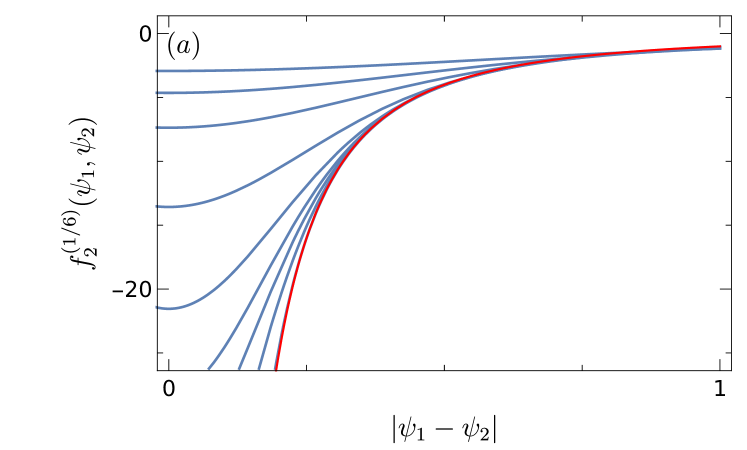
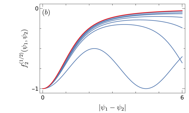
Figure 1: Unfolded two-point function after the rescaling (28) for different values of $N$ (blue). In (a) we used $N=5,10,20,50,100,150,200,300,1000$ and $\alpha=1/6$, in (b) $N=2,5,7,10,15,20,50,100$ and $\alpha=1/2$. For comparison the limit (29) (red).

3.3 Winding Number Distribution

For the discussion to follow, it is useful to cast the random matrix field (6) into an equivalent, but different form. Introducing $s=e^{ip}$ as complex variable on the unit circle, we have

$$K(s)=\frac{s}{2}(K_{1}-iK_{2})+\frac{1}{2s}(K_{1}+iK_{2}).$$ (31)

For the determinant we have

$$\det K(s) =\frac{1}{(2s)^{N}}\det(K_{1}+iK_{2}+s^{2}(K_{1}-iK_{2}))$$ (32)

$$=\frac{\det(K_{1}-iK_{2})}{(2s)^{N}}\prod_{n=1}^{N}\left(s^{2}+z_{n}^{\prime}\right),$$

where the $z_{n}^{\prime}$ are the solution of the generalized eigenvalue problem

$$(K_{1}+iK_{2}){\boldsymbol{v}}_{n}=z_{n}^{\prime}\left(K_{1}-iK_{2}\right){\boldsymbol{v}}_{n}$$ (33)

with eigenvectors ${\boldsymbol{v}}_{n}$. The matrices $K_{1}\pm iK_{2}$ are again Ginibre matrices, implying that the probability distribution of the $z_{n}^{\prime}$ is the one of the spherical ensemble (12). In the sequel, we thus always write $z_{n}$. The winding number in terms of Eq. (31) is

$$W=\frac{1}{2\pi i}\oint_{\left|s\right|=1}ds\frac{1}{\det K(s)}\frac{d}{ds}\det K(s)=\frac{1}{2\pi i}\oint_{\left|s\right|=1}ds\frac{d}{ds}\ln\det K(s).$$ (34)

Obviously, $\det(K_{1}-iK_{2})$ drops out in the integrand. The contour integral yields the difference of zeros and poles of $\det K(s)$ inside the unit circle. From Eq. (32) we infer that it has a pole of order $N$ at zero and that its zeros come in pairs, making their number even. Let $m$ be the number of solutions of Eq. (33) that lie inside the unit circle, then

$$W=2m-N$$ (35)

is the winding number. The number $m$ takes values from $0$ to $N$, thus the winding number lies between $-N$ and $N$. The probability that $m$ eigenvalues are inside the unit circle and the remaining ones outside is

$$r(m)=\int\limits_{\left|z_{1}\right|<1}d[z_{1}]\cdots\int\limits_{\left|z_{m}\right|<1}d[z_{m}]\int\limits_{\left|z_{m+1}\right|>1}d[z_{m+1}]\cdots\int\limits_{\left|z_{N}\right|>1}d[z_{N}]\,G(z).$$ (36)

In Sec. 4 we show that

$$r(m)=\frac{1}{N!}\sum_{\omega\in\mathbb{S}_{N}}\left(\prod_{i=1}^{m}u_{\omega(i)}(N,1)\right)\left(\prod_{i=m+1}^{N}v_{\omega(i)}(N,1)\right),$$ (37)

where the expressions $u_{i}(N,1)$ and $v_{i}(N,1)$ follow from the functions Eq. (3.1). Taking into account the permutation invariance of the eigenvalues inside, respectively outside, the unit circle and using Eq. (35) we find the discrete probability distribution

$$P(W)=r\left(\frac{W+N}{2}\right){N\choose(W+N)/2}$$ (38)

on the integers $W$ between $-N$ and $N$ as the winding number distribution for arbitrary, finite matrix dimension $N$.

Let us now turn to the moments (9) of this distribution. Since the one-point function (27) vanishes, the mean winding number is zero

$$\left\langle W\right\rangle=0.$$ (39)

To arrive at a closed form for $k=2$ we calculate, instead of directly applying the definition (9), the difference in the winding number variance of systems with $(N+1)\times(N+1)$ and $N\times N$ dimensional chiral subblocks. The second moment is given by

$$\left\langle W^{2}\right\rangle\Big{|}_{N}=-\frac{1}{4\pi^{2}}\int_{0}^{2\pi}dp_{1}dp_{2}\ C_{2}(p_{1},p_{2})=\frac{1}{2\pi}\int_{0}^{2\pi}d\varphi\frac{1-\cos^{2N}\varphi}{1-\cos^{2}\varphi},$$ (40)

where we indicate the $N$ dependence. For the difference we find

$$\left\langle W^{2}\right\rangle\Big{|}_{(N+1)}-\left\langle W^{2}\right\rangle\Big{|}_{N} =\frac{1}{2\pi}\int_{0}^{2\pi}d\varphi\cos^{2N}\varphi$$ (41)

$$=\frac{(2N-1)!!}{(2N)!!}=\frac{(2N+1)!!}{(2N)!!}-\frac{(2N-1)!!}{(2N-2)!!},$$

and with $\left\langle W^{2}\right\rangle|_{1}=1$ we obtain

$$\left\langle W^{2}\right\rangle=\frac{(2N-1)!!}{(2N-2)!!}\simeq 2\sqrt{\frac{N}{\pi}}.$$ (42)

The last expression holds for large $N$. Hence, the second moment grows with $\sqrt{N}$, not with $N$. The results (39) and (42) suggests to look at the distribution of $P(W)$ as a function of $W^{2}/\sqrt{N}$ for large $N$. Numerically, we find that it is well described by

$$\frac{P(W)}{P(0)}=\exp\left(-\frac{1}{4}\sqrt{\frac{\pi}{N}}W^{2}\right),$$ (43)

i.e. by a Gaussian distribution.

4 Derivations

In Sec. 4.1 we reformulate the quantity to be ensemble averaged in the $k$-point correlation function (18). We calculate the $N$-point and the $k$-point connected ensemble averages in Secs. 4.2 and 4.3, respectively. The explicit expressions for the one and two-point functions are worked out in Sec. 4.4. In Sec. 4.5 we compute the probability (36) appearing in the discrete winding number distribution (38).

4.1 Reformulation of the Key Expression to be Ensemble Averaged

To perform the calculation of the correlation function (18), it is helpful to rewrite the expression to be ensemble averaged, namely

$$\left\langle\prod_{i=1}^{k}\sum_{n=1}^{N}\frac{1}{q_{i}+z_{n}}\right\rangle,$$ (44)

by pulling out, pictorially speaking, the sums from the angular brackets, i.e. to cast the average (44) into a sum of terms containing only products to be averaged. This requires some work. We use the permutation invariance of the distribution (12) and think of the product of sums as a $k\times N$ lattice. Let the rows be labelled by $i=1,\ldots,k$ and the columns by $n=1,\ldots,N$. As depicted in Fig. 2 for some examples, each term in the product is a

Figure 2: Examples for paths on a $3\times 4$ lattice. Paths ${\boldsymbol{a}}$ and ${\boldsymbol{b}}$ both have the multiindex $(2,1,0,0)$ and are thus equivalent up to permutations in $i$. Path ${\boldsymbol{c}}=(1,1,1,0)$ is the completely connected path along the angle bisector of the lattice. Path ${\boldsymbol{d}}=(0,0,2,1)$ is equal to path ${\boldsymbol{b}}$ as the integration variables $z_{n}$ are permutation invariant.

path through the lattice, obeying the following rules:

• Each row is visited once and only once. This amounts to each $q_{i}$ appearing only once in each of the terms.

• Two paths are considered equal if they visit the same lattice points, irrespective of the order. The points on the lattice are coupled via multiplication, which is commutative.

To each path we assign a multiindex ${\boldsymbol{l}}=(l_{1},\ldots,l_{N})\in\mathbb{N}_{0}^{N}$ of length $\left|{\boldsymbol{l}}\right|=\sum_{n=1}^{N}l_{n}=k$. It describes how many times $l_{n}$ the path has visited the $n$–th column and therefore how many factors including $z_{n}$ appear in the associated term. However, this mapping is not unique. There are in total

$${k\choose{\boldsymbol{l}}}=\frac{k!}{l_{1}!\cdots l_{N}!}$$ (45)

paths sharing the same ${\boldsymbol{l}}$. In the matrix average these terms are equal up to permutations in the $q_{i}$. We take care of this by setting $q_{i}\rightarrow q_{\omega(i)}$ and summing over all permutations

$$\left\langle\prod_{i=1}^{k}\sum_{n=1}^{N}\frac{1}{q_{i}+z_{n}}\right\rangle=\frac{1}{k!}\sum_{\omega\in\mathbb{S}_{k}}\sum_{\left|{\boldsymbol{l}}\right|=k}\left\langle\prod_{i=1}^{k}\frac{1}{q_{\omega(i)}+z_{g_{{\boldsymbol{l}}}(i)}}\right\rangle.$$ (46)

Here, we introduce the step function

$$g_{{\boldsymbol{l}}}(i)=1+\sum_{n=1}^{N}\Theta\left(i-\sum_{j=1}^{n}l_{j}\right),\quad\text{with}\quad\Theta(0)=0,$$ (47)

employing the Heaviside unit step function $\Theta$, to select the correct variables $z_{n}$ for the integration of the corresponding product. We distinguish between different types of paths. In the disconnected paths only one $z_{n}$ appears, which amounts to $l_{n}=k$ for one $n$ and $l_{n}=0$ for all other $n$. We refer to all other paths as connected. Out of the connected paths the ones with $l_{n}\in\{0,1\}$, where each $z_{n}$ may appear only once, stand out. To these paths we refer as completely connected and their contributions may be evaluated via Eq. (21).

Next we consider the permutation invariance of the $z_{n}$. Let $h_{{\boldsymbol{l}}}(i)$ be the function that tallies up the number of integers $i$ appearing in ${\boldsymbol{l}}$. There are

$$\frac{N!}{\prod_{i=1}^{k}h_{{\boldsymbol{l}}}(i)!}$$ (48)

possible ways to permute the $z_{n}$ without changing the ensemble average. We choose the ordered multiindex ${\boldsymbol{l}}$ with $l_{1}\leq\ldots\leq l_{N}$ as a representative for all of these paths. On the $k\times N$ lattice, this amounts to paths below the angle bisector. We thus finally arrive at

$$\left\langle\prod_{i=1}^{k}\sum_{n=1}^{N}\frac{1}{q_{i}+z_{n}}\right\rangle=\frac{1}{k!}\sum_{\omega\in\mathbb{S}_{k}}\sum\limits_{\begin{subarray}{c}l_{1}\leq\ldots\leq l_{N}\\ \left|{\boldsymbol{l}}\right|=k\end{subarray}}{k\choose{\boldsymbol{l}}}\frac{N!}{\prod_{i=1}^{k}h_{{\boldsymbol{l}}}(i)!}\left\langle\prod_{i=1}^{k}\frac{1}{q_{\omega(i)}+z_{g_{{\boldsymbol{l}}}(i)}}\right\rangle.$$ (49)

Indeed, this is a sum over ensemble averages of products only. Generally, any $z_{n}$ may appear $l$ times. To handle this, we use the partial fraction expansion

$$\prod_{i=1}^{l}\frac{1}{q_{i}+z_{n}}=\sum_{i=1}^{l}\frac{1}{\prod_{j\neq i}(q_{j}-q_{i})}\frac{1}{q_{i}+z_{n}},$$ (50)

which reduces the corresponding averages to a sum of completely connected averages. Thus, the resulting expression can again be treated with Eq. (21).

4.2 Calculation of the $N$-Point Connected Ensemble Average

As already pointed out in Sec. 3.1, all connected $k$-point ensemble averages can be, via proper limits, obtained from the connected $N$-point average

$$\left\langle\prod_{n=1}^{N}\frac{1}{q_{n}+z_{n}}\right\rangle=\int d[z]\,G(z)\prod_{n=1}^{N}\frac{1}{q_{n}+z_{n}},$$ (51)

where $G(z)$ is the joint probability density (12) of the spherical ensemble. We use

$$|\Delta_{N}(z)|^{2}=\Delta_{N}(z)\Delta_{N}^{*}(z)=\Delta_{N}(z)\Delta_{N}(z^{*})$$ (52)

and expand the Vandermonde determinant $\Delta_{N}(z)$ in the Laplace form. This yields

$$\left\langle\prod_{n=1}^{N}\frac{1}{q_{n}+z_{n}}\right\rangle =\frac{1}{c_{N}\pi^{N}}\sum_{\omega\in\mathbb{S}_{N}}\text{sgn}\,\omega\int d[z]\Delta_{N}(z^{*})\prod_{n=1}^{N}\frac{z_{n}^{\omega(n)-1}}{\left(1+\left|z_{n}\right|^{2}\right)^{N+1}\left(q_{n}+z_{n}\right)}$$

$$=\frac{1}{c_{N}\pi^{N}}\sum_{\omega\in\mathbb{S}_{N}}\int d[z]\Delta_{N}(z^{*})\prod_{n=1}^{N}\frac{z_{n}^{n-1}}{\left(1+\left|z_{n}\right|^{2}\right)^{N+1}\left(q_{\omega(n)}+z_{n}\right)}$$ (53)

where the second equation follows from renaming the integration variables $z_{n}\rightarrow z_{\omega(n)}$ for each permutation $\omega\in\mathbb{S}_{N}$. The sign $\text{sgn}\,\omega$ of the permutation $\omega$ is canceled by the same sign appearing in $\Delta_{N}(z^{*})$ when changing the integration variables. Inserting the remaining Vandermonde determinant and integrating row by row we obtain Eq. (22) with the function

$$L_{nml}(q) =\int d[z_{n}]\frac{\left(z_{n}^{*}\right)^{m-1}z_{n}^{n-1}}{\left(1+\left|z_{n}\right|^{2}\right)^{N+1}\left(q_{l}+z_{n}\right)}$$

$$=\int_{0}^{\infty}d\rho_{n}\frac{\rho_{n}^{m+n-1}}{(1+\rho_{n}^{2})^{N+1}}\int_{0}^{2\pi}d\vartheta_{n}\frac{e^{i(n-m)\vartheta_{n}}}{q_{l}+\rho_{n}e^{i\vartheta_{n}}},$$ (54)

where we employ polar coordinates $z_{n}=\rho_{n}e^{i\vartheta_{n}}$ in the second equation. The angular integral yields, by virtue of the residue theorem,

$$\int_{0}^{2\pi}d\vartheta_{n}\frac{e^{i(n-m)\vartheta_{n}}}{q_{l}+\rho_{n}e^{i\vartheta_{n}}}=\begin{cases}\displaystyle\frac{2\pi}{q_{l}}\left(-\frac{\rho_{n}}{q_{l}}\right)^{m-n}\qquad&m\geq n,\rho_{n}<q_{l}\\ \displaystyle\frac{2\pi}{\rho_{n}}\left(-\frac{\rho_{n}}{q_{l}}\right)^{m-n+1}\qquad&m<n,\rho_{n}>q_{l}\\ \displaystyle 0\qquad&\text{else}\end{cases}.$$ (55)

Thus we arrive at Eq. (23).

4.3 Reduction to the $k$-Point Connected Ensemble Average

To take the limit (21) we need as an intermediate result a proper limit involving the function $L_{nml}(q_{l})$. As the limit $q_{l}\to\infty$ of the incomplete Beta functions (3.1) gives either unity or zero, the total limit is only non–vanishing if $m=n$,

$$\lim_{q_{l}\rightarrow\infty}q_{l}L_{nml}(q_{l})=\begin{cases}\pi B(m,N-m+1)\qquad&m=n\\ 0\qquad&m\neq n\end{cases}.$$ (56)

We apply this result to reduce the $k$-point connected average, which is, according to Eqs. (21) and (22), a limit of an $N\times N$ determinant. The limit makes all elements in the $\omega^{-1}(n)$–th row vanish except the diagonal element, which is $\pi B(\omega^{-1}(n),N-\omega^{-1}(n)+1)$. We expand the determinant in these elements

$$\left\langle\prod_{n=1}^{k}\frac{1}{q_{n}+z_{n}}\right\rangle =\frac{1}{c_{N}\pi^{k}}\sum_{\omega\in\mathbb{S}_{N}}\left(\prod_{l=k+1}^{N}B(\omega^{-1}(l),N-\omega^{-1}(l)+1)\right)$$

$$\qquad\qquad\qquad\det\left[L_{nm\omega(n)}(q_{\omega(n)})\right]_{n,m=1,\ldots,N}^{n,m\neq\omega^{-1}(l),l=k+1,\ldots,N}.$$ (57)

Interchanging row $n$ with row $\omega^{-1}(n)$ and column $m$ with column $\omega^{-1}(m)$ yields for the right hand side

$$\frac{1}{c_{N}\pi^{k}}\sum_{\omega\in\mathbb{S}_{N}}\left(\prod_{l=k+1}^{N}B(\omega^{-1}(l),N-\omega^{-1}(l)+1)\right)\det\left[L_{\omega^{-1}(n)\omega^{-1}(m)n}(q_{n})\right]_{n,m=1,\ldots,k}$$

$$\qquad\qquad=\frac{1}{c_{N}\pi^{k}}\sum_{\omega\in\mathbb{S}_{N}}\left(\prod_{l=k+1}^{N}B(\omega(l),N-\omega(l)+1)\right)\det\left[L_{\omega(n)\omega(m)n}(q_{n})\right]_{n,m=1,\ldots,k}.$$ (58)

We also used that the order in the sum over the permutations $\omega$ is invariant due to the group property of $\mathbb{S}_{N}$. Thus, we arrive at the result (26).

4.4 Explicit Expressions for the One and Two-Point Correlation Functions

For $k=1$ there are no connected terms. According to Eq. (19) and (49) the one-point function is given by

$$C_{1}(p_{1})=\left\langle y(p_{1})\right\rangle+Nq_{1}=-\frac{N}{\sin^{2}p_{1}}\left\langle\frac{1}{q_{1}+z_{1}}\right\rangle+Nq_{1}.$$ (59)

The average follows from Eq. (26),

$$\left\langle\frac{1}{q_{1}+z_{1}}\right\rangle=\frac{1}{Nq_{1}}\sum_{n=1}^{N}u_{n}(N,q_{1}^{2}).$$ (60)

The incomplete Beta functions (3.1) may be rewritten using integration by parts, we find

$$v_{m}(N,q_{1}^{2})=\sum_{l=0}^{m-1}{N-1-l\choose m-1-l}\frac{(q_{1}^{2})^{m-l-1}}{(1+q_{1}^{2})^{N-l}}.$$ (61)

Using the property (25) the sum in Eq. (60) can be evaluated by means of the binomial theorem, implying

$$\left\langle\frac{1}{q_{1}+z_{1}}\right\rangle=\frac{1}{q_{1}}-\frac{1}{q_{1}(1+q_{1}^{2})}=\sin p_{1}\cos p_{1}.$$ (62)

In the last step we reinserted $q_{1}=\cot p_{1}$. Altogether we arrive at the first of the results (27).

For $k=2$ we apply formulae (19) and (49) and use the vanishing of the one-point function

$$C_{2}(p_{1},p_{2}) =\left\langle y(p_{1})y(p_{2})\right\rangle-N^{2}q_{1}q_{2}$$

$$=\frac{1}{\sin^{2}p_{1}\sin^{2}p_{2}}\left\langle\prod_{i=1}^{2}\sum_{n=1}^{N}\frac{1}{q_{i}+z_{n}}\right\rangle-N^{2}q_{1}q_{2}.$$ (63)

With Eq. (49) we find

$$\left\langle\prod_{i=1}^{2}\sum_{n=1}^{N}\frac{1}{q_{i}+z_{n}}\right\rangle=N\left\langle\frac{1}{q_{1}+z_{1}}\frac{1}{q_{2}+z_{1}}\right\rangle+N(N-1)\left\langle\frac{1}{q_{1}+z_{1}}\frac{1}{q_{2}+z_{2}}\right\rangle.$$ (64)

The connected average is given by (26) and reads

$$\left\langle\frac{1}{q_{1}+z_{1}}\frac{1}{q_{2}+z_{2}}\right\rangle=\frac{1}{N(N-1)}\frac{1}{q_{1}q_{2}}\left(\sum\limits_{\begin{subarray}{c}n,m=1\\ n\neq m\end{subarray}}^{N}u_{n}(N,q_{1}^{2})u_{m}(N,q_{2}^{2})\right.$$

$$\qquad\qquad+\left.\sum\limits_{\begin{subarray}{c}n,m=1\\ n>m\end{subarray}}^{N}\left(\frac{q_{2}}{q_{1}}\right)^{n-m}u_{n}(N,q_{1}^{2})v_{m}(N,q_{2}^{2})+\left(\frac{q_{1}}{q_{2}}\right)^{n-m}v_{n}(N,q_{1}^{2})u_{m}(N,q_{2}^{2})\right)$$ (65)

This expression is readily simplified by using the translation invariance on the parameter manifold. We set $p_{2}=\pi/2$ which amounts to $q_{2}=0$ and find

$$\left\langle\frac{1}{q_{1}+z_{1}}\frac{1}{z_{2}}\right\rangle =\frac{1}{N(N-1)}\frac{1}{q_{1}^{2}}\sum_{n=2}^{N}u_{n}(N,q_{1}^{2})$$

$$=\frac{1}{(N-1)q_{1}^{2}}\left(1-\frac{1}{1+q_{1}^{2}}+\frac{1}{N(1+q_{1}^{2})^{N}}-\frac{1}{N}\right).$$ (66)

For the disconnected average we employ the partial fraction expansion (50) and Eq. (62),

$$\left\langle\frac{1}{q_{1}+z_{1}}\frac{1}{z_{1}}\right\rangle=-\frac{1}{q_{1}}\left(\left\langle\frac{1}{q_{1}+z_{1}}\right\rangle-\left\langle\frac{1}{z_{1}}\right\rangle\right)=-\frac{1}{1+q_{1}^{2}}.$$ (67)

Reinserting $q_{1}=\cot p_{1}$ yields

$$C_{2}\left(p_{1},\frac{\pi}{2}\right)=-\frac{1-\cos^{2N}p_{1}}{1-\cos^{2}p_{1}}$$ (68)

or, equivalently, the second of the results (27).

4.5 Calculation of the Probability $r(m)$

For the discrete winding number distribution (38) we need to compute the probability (36). The calculation is similar to the one in Sec. 4.2. Inserting the probability density (12), treating the Vandermonde determinants as in Sec. 4.2 and renaming the integration variables $z_{n}\rightarrow z_{\omega(n)}$, we have

$$r(m) =\frac{1}{c_{N}\pi^{N}}\sum_{\omega\in\mathbb{S}_{N}}\text{sgn}\,\omega\int\limits_{\left|z_{\omega(1)}\right|<1}d[z_{1}]\cdots\int\limits_{\left|z_{\omega(m)}\right|<1}d[z_{m}]$$

$$\qquad\qquad\int\limits_{\left|z_{\omega(m+1)}\right|>1}d[z_{m+1}]\cdots\int\limits_{\left|z_{\omega(N)}\right|>1}d[z_{N}]\,\prod_{n=1}^{N}\frac{z_{n}^{n-1}(z_{n}^{*})^{\omega(n)-1}}{(1+\left|z_{n}\right|^{2})^{N+1}}.$$ (69)

With polar coordinates $z_{n}=\rho_{n}e^{i\vartheta_{n}}$ we find Kronecker deltas for the angular integrals,

$$\int_{0}^{2\pi}d\vartheta_{n}e^{i(n-\omega(n))\vartheta_{n}}=2\pi\delta_{n\omega(n)}.$$ (70)

Thus, only the unit permutation $\omega=1\!\!1$ contributes. The radial integrals are given by the functions (3.1) for $q_{l}=1$. Altogether we arrive at formula (37).

5 Conclusions

We studied the winding number in a model of parameter dependent chiral random matrices. This seems to be the first time that statistical topology for a chiral symmetry class has been studied in such a schematic model. Apart form the conceptual importance, the winding number has concrete physics interpretations, for example, as the topological index belonging to gapped phases of fermions. We found that the joint probability density of the complex eigenvalues in our model coincides with that of the spherical ensemble which is known in the literature. We used it to address the new questions of statistical topology, we analytically calculated the discrete probability distribution of the winding numbers, as well as the parametric correlations functions of the winding number density. We derived a closed formula for the former and arrived for the latter at explicit determinant expressions for certain correlation functions of arbitrary order which allow for a construction of the winding number density correlations functions. We constructed the one and two-point functions. All our results involve incomplete Beta functions which are fairly simple.

As Random Matrix Theory is widely known to provide universal results for spectral statistics and certain parametric statistics, we are confident that our results hold universal information as well. To reveal it, we carried out an unfolding procedure similar to the one in the above contexts. Remarkably, we found different scaling limits. We expect our results for the unfolded two-point correlation function to be universal.

Our results, namely the implied universality of the correlation function and the Gaussian distribution of the topological index, are analogous to the ones obtained numerically in the case of the adiabatic curvature and the Chern number [26].

References

- [1] Alexander Altland and Martin R. Zirnbauer. Nonstandard symmetry classes in mesoscopic normal-superconducting hybrid structures. Phys. Rev. B, 55:1142–1161, Jan 1997.
- [2] P. Heinzner, A. Huckleberry, and M. R. Zirnbauer. Symmetry classes of disordered fermions. Communications in Mathematical Physics, 257:725–771, 2005.
- [3] Alexei Kitaev. Periodic table for topological insulators and superconductors. AIP Conference Proceedings, 1134(1):22–30, 2009.
- [4] Ching-Kai Chiu, Jeffrey C. Y. Teo, Andreas P. Schnyder, and Shinsei Ryu. Classification of topological quantum matter with symmetries. Rev. Mod. Phys., 88:035005, Aug 2016.
- [5] R. Oppermann. Anderson localization problems in gapless superconducting phases. Physica A: Statistical Mechanics and its Applications, 167(1):301–312, 1990.
- [6] Jacobus Verbaarschot. Spectrum of the qcd dirac operator and chiral random matrix theory. Phys. Rev. Lett., 72:2531–2533, Apr 1994.
- [7] Thomas Guhr, Axel Müller-Groeling, and Hans A. Weidenmüller. Random-matrix theories in quantum physics: common concepts. Phys. Rep., 299(4):189–425, 1998.
- [8] Madan Lal Mehta. Random Matrices. Academic Press, 2004.
- [9] J.J.M. Verbaarschot and T. Wettig. Random matrix theory and chiral symmetry in qcd. Annual Review of Nuclear and Particle Science, 50(1):343–410, 2000.
- [10] E.V. Shuryak and J.J.M. Verbaarschot. Random matrix theory and spectral sum rules for the dirac operator in qcd. Nuclear Physics A, 560(1):306–320, 1993.
- [11] T. Wettig, A. Schäfer, and H.A. Weidenmüller. The chiral phase transition and random matrix models. Nuclear Physics A, 610:492–499, 1996. Quark Matter ’96.
- [12] T. Wettig, A. Schäfer, and H.A Weidenmüller. The chiral phase transition in a random matrix model with molecular correlations. Physics Letters B, 367(1):28–34, 1996.
- [13] A. D. Jackson and J. J. M. Verbaarschot. Random matrix model for chiral symmetry breaking. Phys. Rev. D, 53:7223–7230, Jun 1996.
- [14] J. J. M. Verbaarschot and I. Zahed. Spectral density of the qcd dirac operator near zero virtuality. Phys. Rev. Lett., 70:3852–3855, Jun 1993.
- [15] T. Guhr, T. Wilke, and H. A. Weidenmüller. Stochastic field theory for a dirac particle propagating in gauge field disorder. Phys. Rev. Lett., 85:2252–2255, Sep 2000.
- [16] Constantia Alexandrou, Andreas Athenodorou, Krzysztof Cichy, Arthur Dromard, Elena Garcia-Ramos, Karl Jansen, Urs Wenger, and Falk Zimmermann. Comparison of topological charge definitions in lattice QCD. The European Physical Journal C, 80(5), may 2020.
- [17] Martin R. Zirnbauer. Particle–hole symmetries in condensed matter. Journal of Mathematical Physics, 62(2):021101, 2021.
- [18] Renate Gade. Anderson localization for sublattice models. Nuclear Physics B, 398(3):499–515, 1993.
- [19] C. W. J. Beenakker. Random-matrix theory of majorana fermions and topological superconductors. Rev. Mod. Phys., 87:1037–1066, Sep 2015.
- [20] Bo-Hung Chen and Dah-Wei Chiou. An elementary rigorous proof of bulk-boundary correspondence in the generalized su-schrieffer-heeger model. Physics Letters A, 384(7):126168, 2020.
- [21] Jacob Shapiro. The bulk-edge correspondence in three simple cases. Reviews in Mathematical Physics, 32(03):2030003, 2020.
- [22] Jason Alicea. New directions in the pursuit of majorana fermions in solid state systems. Reports on Progress in Physics, 75(7):076501, jun 2012.
- [23] Ian Mondragon-Shem, Taylor L. Hughes, Juntao Song, and Emil Prodan. Topological criticality in the chiral-symmetric aiii class at strong disorder. Phys. Rev. Lett., 113:046802, Jul 2014.
- [24] Alexander Altland, Dmitry Bagrets, and Alex Kamenev. Topology versus anderson localization: Nonperturbative solutions in one dimension. Phys. Rev. B, 91:085429, Feb 2015.
- [25] Paul N. Walker and Michael Wilkinson. Universal fluctuations of chern integers. Phys. Rev. Lett., 74:4055–4058, May 1995.
- [26] Omri Gat and Michael Wilkinson. Correlations of quantum curvature and variance of Chern numbers. SciPost Phys., 10:149, 2021.
- [27] C.W.J. Beenakker and B. Rejaei. Random-matrix theory of parametric correlations in the spectra of disordered metals and chaotic billiards. Physica A: Statistical Mechanics and its Applications, 203(1):61–90, 1994.
- [28] B. D. Simons and Boris L. Altshuler. Universal velocity correlations in disordered and chaotic systems. Phys. Rev. Lett., 70:4063–4066, Jun 1993.
- [29] B. D. Simons and B. L. Altshuler. Universalities in the spectra of disordered and chaotic systems. Phys. Rev. B, 48:5422–5438, Aug 1993.
- [30] Andreas P. Schnyder, Shinsei Ryu, Akira Furusaki, and Andreas W. W. Ludwig. Classification of topological insulators and superconductors in three spatial dimensions. Phys. Rev. B, 78:195125, Nov 2008.
- [31] Jean Ginibre. Statistical ensembles of complex, quaternion, and real matrices. Journal of Mathematical Physics, 6(3):440–449, 1965.
- [32] Maria Maffei, Alexandre Dauphin, Filippo Cardano, Maciej Lewenstein, and Pietro Massignan. Topological characterization of chiral models through their long time dynamics. New Journal of Physics, 20(1):013023, jan 2018.
- [33] János K. Asbóth, László Oroszlány, and András Pályi. A Short Course on Topological Insulators. Springer International Publishing, 2016.
- [34] Peter J Forrester and Manjunath Krishnapur. Derivation of an eigenvalue probability density function relating to the poincaré disk. Journal of Physics A: Mathematical and Theoretical, 42(38):385204, sep 2009.
- [35] NIST Digital Library of Mathematical Functions. http://dlmf.nist.gov/, Release 1.1.3 of 2021-09-15. F. W. J. Olver, A. B. Olde Daalhuis, D. W. Lozier, B. I. Schneider, R. F. Boisvert, C. W. Clark, B. R. Miller, B. V. Saunders, H. S. Cohl, and M. A. McClain, eds.