Probing the Electron-to-Proton Mass Ratio Gradient in the Milky Way with Class I Methanol Masers

Abstract

We estimate limits on non-universal coupling of hypothetical hidden fields to standard matter by evaluating the fractional changes in the electron-to-proton mass ratio, $\mu=m_{\rm e}/m_{\rm p}$, based on observations of Class I methanol masers distributed in the Milky Way disk over the range of the galactocentric distances $4\;\raise 1.29167pt\hbox{$<$\kern-7.5pt\raise-4.73611pt\hbox{$\sim$}}\;R\;\raise 1.29167pt\hbox{$<$\kern-7.5pt\raise-4.73611pt\hbox{$\sim$}}\;12$ kpc. The velocity offsets $\Delta V=V_{44}-V_{95}$ measured between the 44 and 95 GHz methanol lines provide, so far, one of the most stringent constraints on the spatial gradient $k_{\mu}\equiv d(\Delta\mu/\mu)/dR<2\times 10^{-9}$ kpc^-1 and the upper limit on $\Delta\mu/\mu$ $<2\times 10^{-8}$, where $\Delta\mu/\mu$ = $(\mu_{\rm\scriptscriptstyle obs}-\mu_{\rm\scriptscriptstyle lab})/\mu_{\rm\scriptscriptstyle lab}$. We also find that the offsets $\Delta V$ are clustered into two groups which are separated by $\delta_{\scriptscriptstyle\Delta V}=0.022\pm 0.003$ km s^-1 ($1\sigma$ C.L.). The grouping is most probably due to the dominance of different hyperfine transitions in the 44 and 95 GHz methanol maser emission. Which transition becomes favored is determined by an alignment (polarization) of the nuclear spins of the four hydrogen atoms in the methanol molecule. This result confirms that there are preferred hyperfine transitions involved in the methanol maser action.

1 Introduction

A variety of theories for the dark sector (dark matter and dark energy) suppose the existence of hidden fields which couple non-universally to the Standard Model, SM (for reviews, see Uzan 2011; Marsh 2016; Battaglieri et al. 2017; Hui et al. 2017; Irastorza & Redondo 2018; Terazawa 2018; Beacham et al. 2019; Ahmed et al. 2019). Such coupling would modulate the fermion masses in different ways thus changing their ratios. In particular, this relates to the fundamental constant of particle physics – the electron-to-proton mass ratio, $\mu=m_{\rm e}/m_{\rm p}$, – where $m_{\rm e}$ is directly determined by the coupling to the Higgs-like field(s), whereas the main input to $m_{\rm p}$ comes from the binding energy of quarks. Hence, measurements of $\mu$ can serve as a tool to probe the coupling between the SM and dark sector. New fields are predicted to be ultralight (Compton wavelengths $\lambda\sim 1$ kpc) and/or to change their values depending on the environmental parameters such as gravitational potential of baryonic matter or local baryonic mass density (e.g., Damour & Polyakov 1994; Khoury & Weltman 2004; Olive & Pospelov 2008; Brax 2018). This makes astronomical objects preferable targets in corresponding studies.

Measurements of fractional changes in $\mu$,

$$\frac{\Delta\mu}{\mu}=\frac{\mu_{\rm\scriptscriptstyle obs}-\mu_{\rm\scriptscriptstyle lab}}{\mu_{\rm\scriptscriptstyle lab}},$$ (1)

in astronomical objects are based on the fact that the molecular electron-vibro-rotational transitions have specific dependences on $\mu$ (Thompson 1975) and different sensitivities to $\mu$-variations (Varshalovich & Levshakov 1993; Flambaum & Kozlov 2007; Levshakov et al. 2011; Jansen et al. 2011; Patra et al. 2018). For a given molecular transition frequency $f$, the dimensionless sensitivity coefficient to a possible variation of $\mu$ is defined as

$$Q=\frac{df/f}{d\mu/\mu}\,.$$ (2)

The coefficients $Q$ take positive or negative signs and values ranging between $\sim 10^{-2}$ for H₂ and $\sim 10$s for CH₃OH and other molecules (for a review see, e.g., Kozlov & Levshakov 2013). The fractional changes in $\mu$ can be measured using any pair of lines of co-spatially distributed molecular transitions ($i,j$) with different values of $Q$ (Levshakov et al. 2011):

$$\frac{\Delta\mu}{\mu}=\frac{V_{j}-V_{i}}{c(Q_{i}-Q_{j})},$$ (3)

where $V_{j}$ and $V_{i}$ are the LSR radial velocities of molecular transitions with sensitivity coefficients $Q_{j}$ and $Q_{i}$, and $c$ is the speed of light. It is to note that spectral observations with modern facilities provide an unprecedented accuracy in measurements of molecular transitions and, hence, in $\Delta\mu/\mu$. Additional advantages are the relative simplicity of interpretation of the obtained results and a restricted number of sources of systematic errors (cf., e.g., Touboul et al. 2020).

Presently, the most stringent limit on $\Delta\mu/\mu$, $\Delta\mu/\mu$ $<7\times 10^{-9}$ (hereafter a $1\sigma$ confidence level is used), was obtained from high resolution spectral observations of Milky Way’s cold molecular cores in lines of NH₃, HC₃N, HC₅N, HC₇N, and N₂H⁺ at the Effelsberg 100-m, Medicina 32-m, and Nobeyama 45-m radio telescopes (Levshakov et al. 2010a,b; Levshakov et al. 2013, hereafter L13). Additionally, observations of the dense dark cloud core L1498 in thermal $E$- and $A$-type methanol CH₃OH lines at the IRAM 30-m telescope gave the upper limit of $\Delta\mu/\mu$ $<2\times 10^{-8}$ (Daprá et al. 2017, hereafter D17). In these studies, all molecular cores were located within a 300 pc radius from the Sun, which is insufficient to detect the predicted gradients of hidden ultralight fields: to probe the SM–dark sector coupling, observations of targets spaced apart by distances of kiloparsecs are required.

Such targets are objects of the present paper. We aim at obtaining the $\Delta\mu/\mu$ estimate in the Milky Way disk utilizing narrow emission lines of bright Class I methanol (CH₃OH) masers from the northern Galactic hemisphere distributed over the galactocentric distance range of $4\;\raise 1.29167pt\hbox{$<$\kern-7.5pt\raise-4.73611pt\hbox{$\sim$}}\;R\;\raise 1.29167pt\hbox{$<$\kern-7.5pt\raise-4.73611pt\hbox{$\sim$}}\;12$ kpc.

Methanol masers are usually classified into two types: Class I and Class II. The first type of sources is offset by $\sim 1$ pc from star formation signposts and mostly the result from collisional excitation (Menten 1991a,b; Cragg et al. 2005; Leurini et al. 2016). The sources are associated with shocks caused by molecular outflows, expansion of H ii regions, and cloud-cloud interactions (Kurtz et al. 2004; Voronkov et al. 2006, 2010, 2014). Masers of the second type are found in the closest environment of massive young stellar objects and are pumped by the reprocessed dust continuum radiation from these sources. The Class II methanol masers at 6.2 and 12.2 GHz were used by Ellingsen et al. (2011) to limit $\mu$-variations at the level $|\Delta\mu/\mu|<2.7\times 10^{-8}$. The advantages of using Class I methanol masers for the $\Delta\mu/\mu$ measurements are the following:

• They belong to a large population of Galactic emitters which are distributed across the Galactic plane towards both the Galactic centre and anti-centre. This enables us to scan $\Delta\mu/\mu$ over a large spatial range.

• The maser lines are strong and narrow (non-thermal) and, thus, their radial velocities can be measured with high precision.

• Methanol transitions show large differences in the sensitivity coefficients (denominator in Eq. 3). This naturally decreases uncertainties of the $\Delta\mu/\mu$ estimate.

• Class I masers are stable, i.e., do not exhibit flux variability at time intervals $\sim 1$ yr in contrast to Class II methanol masers which show greater temporal variability.

We estimate the fractional changes in $\mu$ using the Class I $A$-type methanol transitions at 44 and 95 GHz. The emission in these transitions is closely associated and traces the same spots (Val’tts et al. 2000; Voronkov et al. 2014; Leurini et al. 2016). This minimizes the Doppler noise, which are random shifts of spectral line positions caused by possible spatial segregation and kinematic effects. In addition to this component, which is stochastic, the total error budget of the measured radial velocity, $V_{\scriptscriptstyle\rm LSR}$, of a given spectral line contains also a systematic error related to the uncertainty in the laboratory values of rest frequencies. The laboratory frequencies of the 44 and 95 GHz transitions are presently measured with an error of $\sim 10$ kHz (Tsunekawa et al. 1995; Müller et al. 2004). This translates into systematic errors of $V_{\scriptscriptstyle\rm LSR}$ as great as $\sim 10$ m s^-1, restricting the limit on $\Delta\mu/\mu$ at the level of $10^{-8}$, i.e., the level already reached in the most accurate $\Delta\mu/\mu$ estimates up-to-now.

In principle, it is technically possible to measure the laboratory frequencies with accuracy $\sim 1$ kHz. However, the problem is more complicated. Namely, the molecule CH₃OH possesses an underlying hyperfine structure scaled over the same $\sim 10$ kHz (Hougen et al. 1991; Coudert et al. 2015; Belov et al. 2016; Lankhaar et al. 2016). The hyperfine splitting can only be partly resolved in the laboratory and is completely convolved in astrophysical observations. If emission is purely thermal, then the barycentre of the convolved profile is more or less stable and its error is localized within the kHz uncertainty interval (D17). If, however, emission is due to masing effects, then, as shown in Lankhaar et al. (2018), population inversion may be enhanced for some hyperfine transitions, while suppressed for others. The physical mechanisms leading to the favoured pumping of this or that hyperfine sublevel are not yet clear enough. As a result, the barycentre of the convolved profile will shift with an amplitude of $\sim 10$ kHz depending on the physical environment. The investigation of this additional systematics is another purpose of the present paper.

2 Observations and target selection

We use simultaneous observations of the 44 GHz ($7_{0}-6_{1}$ A⁺) and 95 GHz ($8_{0}-7_{1}$ A⁺) Class I methanol masers from the so-called Red MSX Source (RMS) catalogue observed by Kim et al. (2018) (hereafter K18), and from the Bolocam Galactic Plane Survey (BGPS) sources observed by Yang et al. (2020) (hereafter Y20). Both surveys were performed with the Korean VLBI Network (KVN) 21-m telescopes in single-dish telescope mode. The multifrequency receiving systems at each telescope allow us to observe 44 and 95 GHz methanol transitions at the same time, and with velocity scales defined in the same way. These two advantages are not being met by any other data set. Details of these observations are given in the original papers, here we repeat only those relevant to the present study.

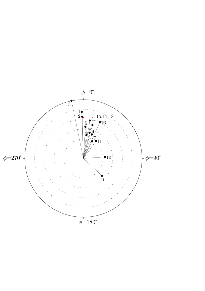
Figure 1: Location of the methanol masers (marked by numbers in accord with Table 1) in projection onto the Galactic plane. The concentric circles give the galactocentric distances starting from 4 kpc; the increment is 2 kpc. The Galactic centre is at coordinates $(R,\phi)=(0,0)$, and the Sun (red dot) is at coordinates $(R,\phi)$ = (8.34 kpc,0), as adopted by Mège et al. (2021).

Both the K18 and Y20 works were surveys aimed in the first place at the discovery of new methanol masers. Because of that the signal-to-noise ratio (S/N) in the majority of targets was not high enough to deduce the radial velocities with the required accuracy of $\sim$ 10s m s^-1. As a result, only 7 objects from 229 maser sources of K18 and 11 objects from 144 sources of Y20 turned out to be suitable for our purposes; the selected targets are listed in Table 1. Their spatial distribution in the Galactic disk is shown in Fig. 1. The objects lie at low Galactic latitudes $-2.6^{\circ}<b<2.8^{\circ}$ and are located towards both the Galactic centre and anti-centre at distances $D_{a}\leq 4.7$ kpc (anticentre) and $D_{c}\leq 12.3$ kpc (centre) from the Sun. Thus, the maximum scale covered is approximately 16 kpc which is comparable to the Galactic optical radius.

Both the K18 and Y20 surveys report a remarkable strong correlation between methanol peak velocities for the 44 and 95 GHz transitions:

$$V_{\rm pk,95}=(0.98\pm 0.05)V_{\rm pk,44}-(0.01\pm 0.010),$$ (4)

and

$$V_{\rm pk,95}=(0.9998\pm 0.0010)V_{\rm pk,44}-(0.0470\pm 0.0614),$$ (5)

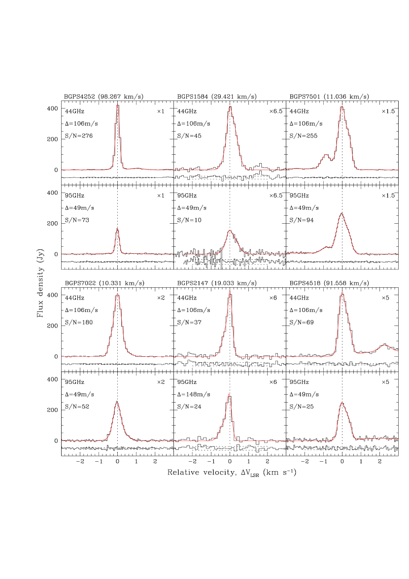
Figure 4: Same as Fig. 3, but for the BGPS (Bolocam Galactic Plane Survey) sources taken from Yang et al. (2020) and listed in Table 5. The BGPS catalogue (version of 1.0.1) can be found at https://irsa.ipac.caltech.edu/data/BOLOCAM_GPS/tables/bolocam_gps_v1_0_1.tbl

respectively. For the mean value of ${V}_{\rm pk,44}\simeq 75$ km s^-1 (see Fig. 4 in Y20) the relation (5) provides for the offset $\Delta V=V_{\rm pk,44}-V_{\rm pk,95}$ an error $\sigma_{\scriptscriptstyle\Delta V}\sim 0.1$ km s^-1, which transforms into an upper limit on $\Delta\mu/\mu$ $<10^{-7}$ in accord with Eq.(3) where $Q_{95}-Q_{44}=3.3$ (see Subsec. 3.3). Below we show how a more stringent limit on $\Delta\mu/\mu$  can be deduced from the existent datasets.

In K18, the original channel widths were $\Delta_{\rm ch}=0.053$ km s^-1 at 44 GHz, and 0.025 km s^-1 at 95 GHz, whereas in Y20, they were two times larger, $\Delta_{\rm ch}=0.106$ km s^-1 at 44 GHz, and 0.049 km s^-1 at 95 GHz. The peak flux densities, $F_{44}$ and $F_{95}$, indicated in Table 1, vary between 12 Jy (95 GHz, RMS153) and 420 Jy (44 GHz, BGPS4252) providing signal-to-noise ratios between S/N = 10 and S/N = 276. Both the signal-to-noise ratio and channel width are crucial for our analysis since they define the final uncertainty of the line position. Namely, an expected statistical uncertainty of the centre of a Gaussian-like line profile is given by (e.g., Landman et al. 1982):

$$\sigma_{0}\simeq\frac{0.7\Delta_{\rm ch}}{\rm S/N}\sqrt{n},$$ (6)

where $n={\rm FWHM}/\Delta_{\rm ch}$ is the line’s full width at half maximum (FWHM) in units of channels. With a typical line width (FWHM) for the methanol lines in question of $\sim 0.5$ km s^-1, one obtains for the marginal values of S/N = 10 and 276 the following errors: $\sigma_{0}\simeq 0.014$ km s^-1 ($\Delta_{\rm ch}=0.074$ km s^-1) and $\sigma_{0}\simeq 0.0006$ km s^-1 ($\Delta_{\rm ch}=0.106$ km s^-1).

The adopted rest frequencies 44069.430 MHz ($7_{0}-6_{1}$ A⁺) from Pickett et al. (1998) and 95169.463 MHz ($8_{0}-7_{1}$ A⁺) from Müller et al. (2004) were utilized in the original papers of K18 and Y20. Note that these frequencies differ from those recommended by NIST, NRAO, JPL, and CDMS (see Table 2).

3 Analysis

3.1 Method

At first, we determined the baseline for each original spectrum by choosing spectral windows without emission lines and/or noise spikes and then calculating the mean flux densities $F_{i}$ along with their rms uncertainties $\sigma_{i}$ for each spectral window. Using spline interpolation through this set of pairs $\{F_{i},\sigma_{i}\}$ we calculated a baseline which was subtracted from the spectrum. Then, the mean value of the rms uncertainties, $\sigma_{\rm rms}$, was determined and assigned to the whole spectrum.

The radial velocities $V_{\scriptscriptstyle\rm LSR}$ in Eq. 3 are calculated as described in Levshakov et al. (2019). $V_{\scriptscriptstyle\rm LSR}$ is attributed to the line centre which is defined as a point where the first order derivative of the line profile is equal to zero. In order to calculate this extremum point accurately the observed line profile, $f(x)$, is filtered. The filtering function $y(x)$ consists of a sum of $N$ Gaussian subcomponents, parameters of which are calculated by minimization of a $\chi^{2}$ function:

$$\chi^{2}_{\nu}=\frac{1}{\nu}\sum\{[f(x_{i})-y(x_{i})]/\sigma_{\rm rms}\}^{2},$$ (7)

where $\nu$ is the number of degrees of freedom. The number of subcomponents, $N$, is chosen so that the $\chi^{2}_{\nu}$ function is minimized at the level of $\chi^{2}_{\nu}\simeq 1$ to avoid under- or over-fitting of the line profile. The uncertainty of $V_{\scriptscriptstyle\rm LSR}$, $\sigma_{v}$, is determined by three points $\{x_{1},y_{1};x_{2},y_{2};x_{3},y_{3}\}$ with $x_{1}<x_{2}<x_{3}$ which include the flux density peak, $x_{\rm peak}\in(x_{1},x_{3})$:

$$\sigma_{v}=\frac{\sigma_{\rm rms}\cdot\Delta_{\rm ch}}{(y_{1}-2y_{2}+y_{3})^{2}}{\cal K},$$ (8)

where ${\cal K}=\sqrt{(y_{3}-y_{2})^{2}+(y_{1}-y_{3})^{2}+(y_{2}-y_{1})^{2}}$, and the channel width $\Delta_{\rm ch}=x_{2}-x_{1}=x_{3}-x_{2}$.

3.2 Reproducibility of radial velocities

The 44 GHz transition was observed by K18 in two epochs: the first one in 2011, and the second in 2012. The second set of observations included also the 95 GHz line. The one year time lapse can be used to test stability of Class I methanol masers as was mentioned in Sect. 1.

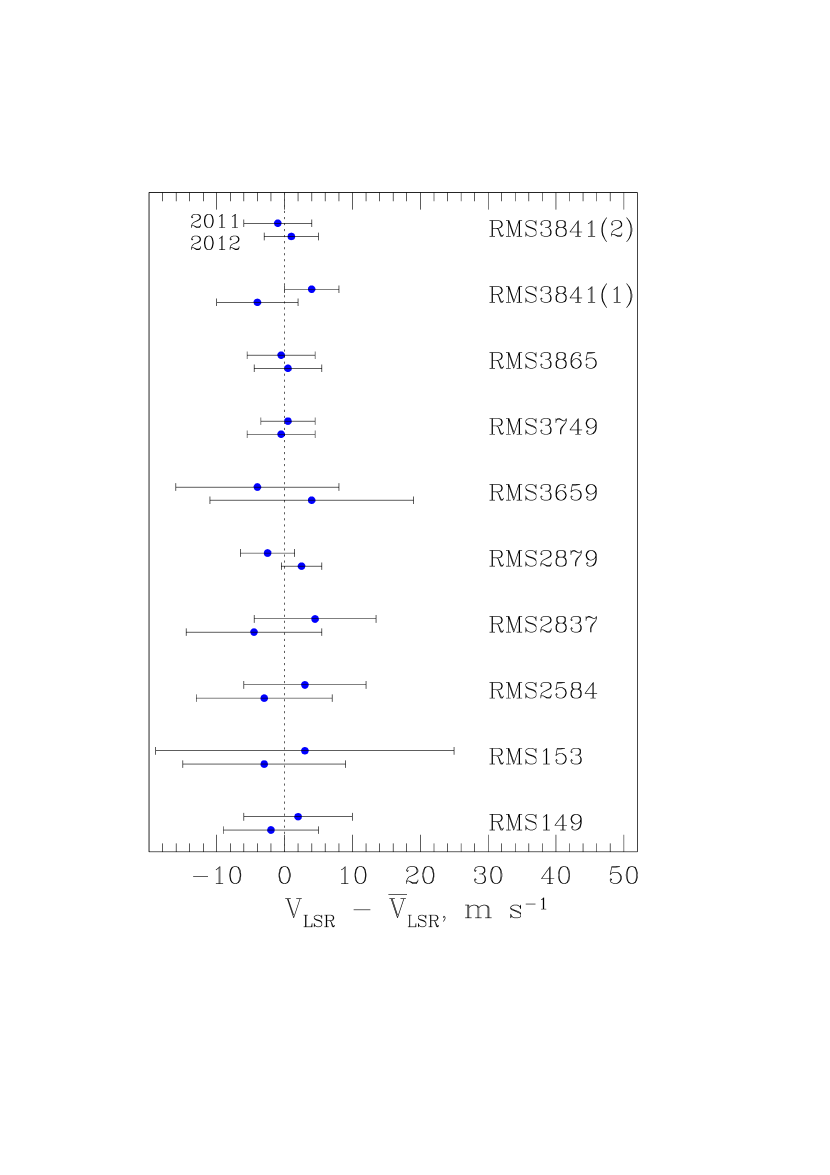
Figure 2: Reproducibility of the methanol line positions illustrated by the relative offsets of the measured $V_{\rm\scriptscriptstyle LSR}$ velocities of the 44 GHz line with respect to the mean value $\bar{V}_{\rm\scriptscriptstyle LSR}$ between the two observational epochs indicated at the left hand upper corner (see Table 3 for details). Error bars represent the experimental uncertainty $(1\sigma)$. The weighted mean of the velocity offsets $\Delta V_{\rm yr}=V_{2011}-V_{2012}$ is $\langle\Delta V_{\rm yr}\rangle_{w}=-1.1\pm 1.6$ m s^-1.

The radial velocities $V_{\rm\scriptscriptstyle LSR}$ of the 44 GHz line measured with respect to the mean value $\bar{V}_{\rm\scriptscriptstyle LSR}$ between the two observational epochs are plotted in Fig. 2, while the individual $V_{\rm\scriptscriptstyle LSR}$ values are listed in Table 3. This table includes 10 velocity offsets between 2011 and 2012 observations towards 9 maser sources (the 44 GHz profile in RMS3841 consists of two narrow subcomponents separated by 0.4 km s^-1). However, in the further analysis we used only 7 targets since the 95 GHz profiles towards RMS2584 and RMS3841 were not good enough for precision measurements of their $V_{\rm\scriptscriptstyle LSR}$ values.

Figure 2 demonstrates stability of the 44 GHz line position for all 10 pairs with the weighted mean $\langle\Delta V_{\rm yr}\rangle_{w}=-1.1\pm 1.6$ m s^-1. Taking this into account, we stack up 44 GHz spectra from both epochs coadding them with weights inversionally proportional to their variances, $\sigma^{2}_{\rm rms}$. The measured radial velocities based on the stacked data are listed in Table 4, second column. Since for the 44 and 95 GHz data, being taken at the same time (in 2012) with the same telescopes, the computations of velocity corrections leading to LSR velocities match each other. Thus stacking does not introduce a statistically significant systematic error.

3.3 Fractional changes in $\mu$

As it follows from Eq. 3, the fractional changes in $\mu$ are defined by the LSR radial velocities of a pair of methanol lines, $V_{i}$ and $V_{j}$, which have different sensitivity coefficients, $Q_{i}$ and $Q_{j}$, to $\mu$-variations.

For the 44 and 95 GHz methanol transitions the sensitivity coefficients were calculated in Jansen et al. (2011) and in Levshakov et al. (2011). Both groups give similar $Q$-values: $Q_{44}=-5.2\pm 0.3$, $Q_{95}=-1.88\pm 0.09$ (Jansen et al.), and $Q_{44}=-5.3\pm 0.6$ and $Q_{95}=-1.9\pm 0.3$ (Levshakov et al.). In our analysis we use $Q_{44}=-5.2$ and $Q_{95}=-1.9$. Their difference $\Delta Q=3.3$ is comparable to the difference between the sensitivity coefficients in the ammonia method where $\Delta Q=3.46$ (Flambaum & Kozlov 2007; Levshakov et al. 2010a).

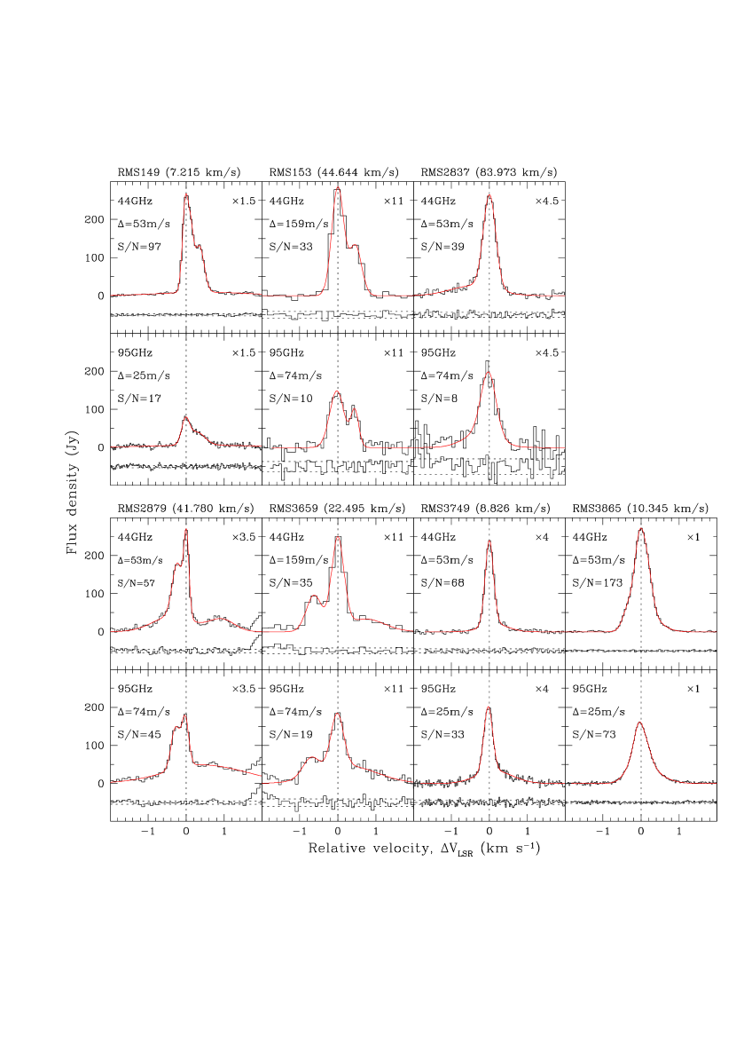
Figure 3: Black histograms are the baseline subtracted emission lines of CH₃OH at 44 GHz and 95 GHz towards RMS sources (Red Midcourse Space Experiment) taken from Kim et al. (2018) and listed in Table 4. The LSR radial velocities are given relative to the peak LSR velocity of the 44 GHz line which is indicated in parentheses after the source name. The fitting curves are shown by red. The residuals are plotted by the lower black histogram (arbitrarily offset for clarity), while the horizontal dotted lines show their $\pm 1\sigma$ boundaries. The signal-to-noise ratio (S/N) per channel at the line peak, the used channel width $\Delta$ (in m s^-1), and the flux density scale factor are depicted in each panel. The vertical dotted line marks the peak position of the 44 GHz line given to indicate small velocity offsets for the 95 GHz line.

The measured LSR radial velocities along with their uncertainties are given in Tables 4 and 5, whilst the fitting procedure is illustrated in Figs. 3 – 5. In these figures, vertical panels represent the 44 GHz (upper panel) and 95 GHz (lower panel) profiles of methanol masers whose names and peak velocities of the 44 GHz line are indicated at the top of each block. Some spectra were smoothed in order to improve the S/N ratio in individual channels and the used channel width is indicated in the corresponding panel.

In all calculations we used the rest frequencies adopted in the original papers of K18 and Y20 (see Table 2): $f^{\rm\scriptscriptstyle P}_{44}=44069.430$ GHz from Pickett et al. (1998), and $f^{\rm\scriptscriptstyle M}_{95}=95169.463$ GHz from Müller et al. (2004). If other sets of the rest frequencies listed in Table 2 would be adopted, then the velocity offsets, $\Delta V=V_{44}-V_{95}$, change as shown in Table 4, columns 4-8. These values were calculated in the following way.

The KVN telescopes adopt the radio definition of radial velocity which is given by

$$V_{\rm\scriptscriptstyle LSR}=c\left(1-\frac{f_{\rm obs}}{f_{\rm lab}}\right),$$ (9)

where $c$ is the speed of light. If we now consider two methanol lines with laboratory rest frequencies $f^{\prime}_{0,i}$ and $f^{\prime}_{0,j}$ (“old” reference frame) which are observed at the corresponding sky frequencies $f_{i}$ and $f_{j}$ and have the LSR radial velocities $V^{\prime}_{i}$ and $V^{\prime}_{j}$, then the difference between the measured velocities of these lines is determined for a new set of laboratory frequencies $f_{0,i}$ and $f_{0,j}$ (“new” reference frame) as

$$\Delta V_{ij}=\Delta V^{\prime}_{ij}+\delta V_{ij},$$ (10)

where $\Delta V^{\prime}_{ij}=V^{\prime}_{i}-V^{\prime}_{j}$ is the velocity offset between the lines $i$ and $j$ in the “old” reference frame, and $\delta V_{ij}$ is the Doppler correction term between the “old” and “new” reference frames:

$$\delta V_{ij}=c\left(\frac{f^{\prime}_{0,j}}{f_{0,j}}-\frac{f^{\prime}_{0,i}}{f_{0,i}}\right).$$ (11)

The absolute values of the weighted mean velocity offsets under different sets of laboratory frequencies $|\langle\Delta V\rangle_{w}|$ range from 0.030 km s^-1 to 0.176 km s^-1 (Table 4). In terms of $\Delta\mu/\mu$ (Eq. 3) these boundaries correspond to $\Delta\mu/\mu$ = $3.0\times 10^{-8}$ and $1.8\times 10^{-7}$, respectively. However, the latter clearly exceeds the upper limits on $\Delta\mu/\mu$ found in the Galaxy: $\Delta\mu/\mu$ $<7\times 10^{-9}$ (L13) and $\Delta\mu/\mu$ $<2\times 10^{-8}$ (D17). This means that the uncertainties in the JPL, NIST, and CDMS catalogues as well as those reported in Tsunekawa et al. (1995) seem to be far too small since the published rest frequencies lead to unrealistically large estimates of $\Delta\mu/\mu$ $\sim 10^{-7}$.

Accounting for all these details, we list in Table 5 only those $V_{\rm\scriptscriptstyle LSR}$ and $\Delta V$ values which are calculated with rest frequencies taken from the original paper of Y20.

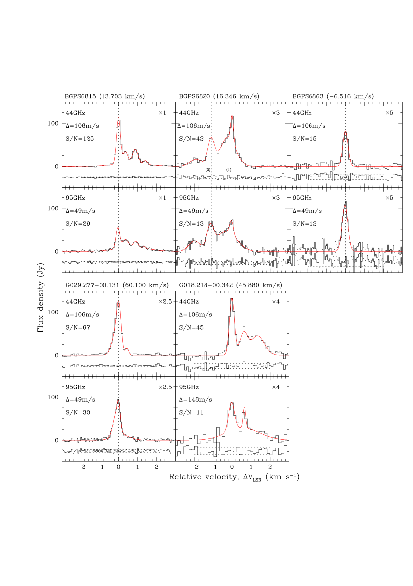
Figure 5: Continuation of Fig. 4

Our final sample consists of 7 sources from K18 and 11 sources from Y20 and the source BGPS6820 provides two peaks (see Fig. 5), i.e., in total we have 19 velocity offsets.

3.4 Spatial gradient of $\Delta\mu/\mu$

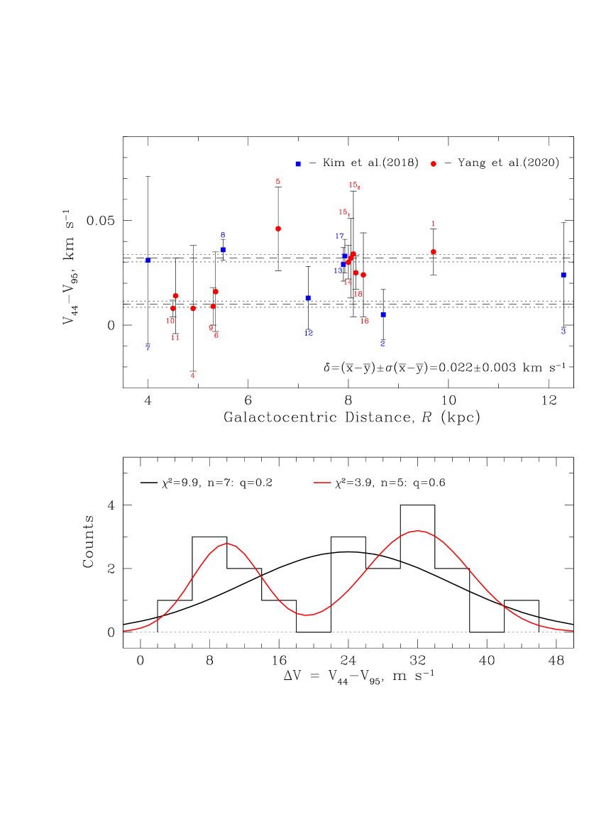
Figure 6: Upper panel. The measured velocity offsets $\Delta V=V_{44}-V_{95}$ against the galactocentric distances of the Class I methanol masers for the rest frequencies of 44069.430 MHz (Pickett et al. 1998) and 95169.463 MHz (Müller et al. 2004). The blue squares and red dots represent the sources from Tables 4 and 5, respectively. The horizontal dashed and dotted lines represent two sample means $\bar{x}=0.032$ km s^-1 and $\bar{y}=0.010$ km s^-1, and their $\pm 1\sigma$ boundaries. Student’s $t$-test supports the revealed difference $\delta$ between two groups of masers at $7.3\sigma$. Lower panel. The binned distribution of $\Delta V$ (histogram) compared to the unimodal (black curve) and bimodal (red curve) distributions. The corresponding $\chi^{2}$ values, the numbers of degrees of freedom $n$, and the quantiles $q$ are shown at the top of the panel. The probability of the bimodal distribution is 60% against 20% for the unimodal distribution in accord with the $\chi^{2}$-test for normality.

For each of the selected targets the measured velocity offset $\Delta V$ = $V_{44}-V_{95}$ is depicted in the upper panel of Fig. 6 against the target’s distance $R$ from the Galactic centre. The blue squares and red dots represent the sources from Tables 4 and 5, respectively. The indicated numbers correspond to the numbering in Table 1. The source BGPS6820 is represented by two red dots $15_{1}$ and $15_{2}$.

It is seen that there is a clustering of points into two groups what hints to the possible bimodality of the underlying distribution of the velocity offsets. This hypothesis is statistically tested (by $\chi^{2}$-criterium) as illustrated in the lower panel of Fig. 6. The unimodal distribution (black curve) with the mean $\langle\Delta V\rangle=0.024$ km s^-1, dispersion $\sigma=0.012$ km s^-1, and the number of degrees of freedom $n=7$ gives $\chi^{2}=9.9$, which corresponds to a significance (probability) of 20%. On the other hand, the bimodal distribution (red curve) with $n=5$, two separate means $\langle\Delta V\rangle_{1}=0.032$ km s^-1, $\langle\Delta V\rangle_{2}=0.010$ km s^-1, and dispersions $\sigma_{1}=0.006$ km s^-1, $\sigma_{2}=0.004$ km s^-1 delivers $\chi^{2}=3.9$ with the significance of 60%. Thus, we separate the data into two subsamples with $N=12$ and $N=7$ points. The corresponding sample means and their $1\sigma$ errors are $\langle\Delta V\rangle_{1}\equiv\bar{x}=0.0316\pm 0.0018$ km s^-1, and $\langle\Delta V\rangle_{2}\equiv\bar{y}=0.0104\pm 0.0015$ km s^-1, (marked by the horizontal dashed and dotted lines in the upper panel of Fig. 6). The weighted means and their errors are similar: $\langle\Delta V\rangle_{1,w}=0.0321\pm 0.0014$ km s^-1, and $\langle\Delta V\rangle_{2,w}=0.0086\pm 0.0009$ km s^-1. The significance of this difference in terms of Student’s $t$-test with $n=17$ degrees of freedom is about $7\sigma$: $\delta=(\bar{x}-\bar{y})\pm\sigma(\bar{x}-\bar{y})=0.022\pm 0.003$ km s^-1.

Additional arguments in support of two groups are that each of them contains points from both the K18 and Y20 surveys and that there is no correlation with the galactocentric distances, $R$, and/or the bolometric luminosities, $L_{\rm bol}$, listed in Table 1. This minimizes the probability of possible observational selection and systematic biases.

We note that the revealed bimodality does not depend on the rest frequencies of the 44 and 95 GHz lines since any combination of the rest frequencies listed in Table 2 would simply lead to a parallel shift of all points in the upper panel of Fig. 6 along the $Y$-axis. With our adopted set of the rest frequencies the weighted means for $\Delta\mu/\mu$ for each group are the following: $(\Delta\mu/\mu)_{1,w}=(32.5\pm 1.4)\times 10^{-9}$ and $(\Delta\mu/\mu)_{2,w}=(8.6\pm 0.9)\times 10^{-9}$.

Table 1 shows that the targets are distributed at galactocentric distances $4.0\;\raise 1.29167pt\hbox{$<$\kern-7.5pt\raise-4.73611pt\hbox{$\sim$}}\;R\;\raise 1.29167pt\hbox{$<$\kern-7.5pt\raise-4.73611pt\hbox{$\sim$}}\;12.3$ kpc. In this range, the input of the baryonic gravitational potential to the circular velocity of the Galactic rotation falls from 60-70% at $R\sim 4$ kpc to 30-50% at $R\sim 12$ kpc, whereas the input attributed to the dark matter increases correspondingly (e.g., Eilers et al. 2019; Bobylev et al. 2021; Nitschai et al. 2021). If the putative coupling between the baryonic and dark matter exists, then one can expect some dependence of $\Delta\mu/\mu$ on $R$.

The linear regression analysis of the velocity offsets for both groups returns similar constraints on the gradient of $\Delta V$: $(k_{\scriptscriptstyle\Delta V})_{1}=-0.0015\pm 0.0020$ km s^-1 kpc^-1 in the range $4.0\;\raise 1.29167pt\hbox{$<$\kern-7.5pt\raise-4.73611pt\hbox{$\sim$}}\;R\;\raise 1.29167pt\hbox{$<$\kern-7.5pt\raise-4.73611pt\hbox{$\sim$}}\;12.3$ kpc, and $(k_{\scriptscriptstyle\Delta V})_{2}=-0.0002\pm 0.0027$ km s^-1 kpc^-1 in the range $4.5\;\raise 1.29167pt\hbox{$<$\kern-7.5pt\raise-4.73611pt\hbox{$\sim$}}\;R\;\raise 1.29167pt\hbox{$<$\kern-7.5pt\raise-4.73611pt\hbox{$\sim$}}\;8.7$ kpc, what gives an upper limit on the gradient $k_{\mu}$ of $\Delta\mu/\mu$ in the Milky Way disk: $k_{\mu}<2\times 10^{-9}$ kpc^-1. With this gradient, we constrain the value of $\Delta\mu/\mu$ in the range $4.0\;\raise 1.29167pt\hbox{$<$\kern-7.5pt\raise-4.73611pt\hbox{$\sim$}}\;R\;\raise 1.29167pt\hbox{$<$\kern-7.5pt\raise-4.73611pt\hbox{$\sim$}}\;12.3$ kpc as $\Delta\mu/\mu$ $<2\times 10^{-8}$. This estimate is only slightly better than that reported by D17 and Ellingsen et al. (2011), but it is three times less tight as in L13 due to poor statistics of our targets.

It is interesting to compare the obtained $k_{\mu}$ estimate with corresponding values from other experiments. For example, the MICROSCOPE satellite mission also aimed at measuring the effects of possible non-universal coupling, but in a completely different way: it placed two masses of different composition (titanium and platinum alloys) on an orbit around the Earth and measured their circular acceleration (torsion balance). The reported upper limit on the non-standard coupling is $<10^{-14}$ (Touboul et al. 2020). With our estimate of the spatial gradient and the assumption of its isotropy one obtains for the MICROSCOPE distance from the Earth centre (7000 km) an upper limit on the non-standard coupling of $<4\times 10^{-22}$ which is tighter by eight orders of magnitude. This shows once more the advantages of astrophysical spectroscopic methods.

4 Maser action in the 44 and 95 GHz hyperfine components

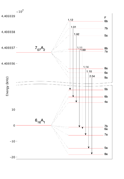
Figure 7: Hyperfine structure of the torsion-rotation levels of the 44 GHz ($7_{07}A_{2}\rightarrow 6_{16}A_{1}$) transition of methanol as calculated in Lankhaar et al. (2016). The energy of the $6_{16}A_{1}$ torsion-rotation level is set to zero. The Y-axis is broken in order to show both the hyperfine interactions ($\Delta E\sim 10$ kHz) and the torsion-rotational energy difference (here $\Delta E\sim 44$ GHz). The torsion-rotation central frequency $f_{0}=44069.367$ MHz is adopted from Xu et al. (2008). Arrows indicate the strongest hyperfine transitions with $\Delta F=\Delta J=1$, with the Einstein $A$ coefficients (in $10^{-7}$ s^-1) indicated above (see Table 6).

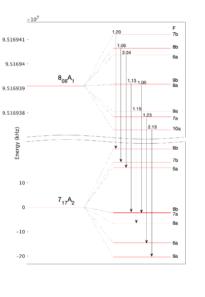
Figure 8: Hyperfine structure of the torsion-rotation levels of the 95 GHz ($8_{08}A_{1}\rightarrow 7_{17}A_{2}$) transition of methanol as calculated in Lankhaar et al. (2016). The energy of the $7_{17}A_{2}$ torsion-rotation level is set to zero. The Y-axis is broken in order to show both the hyperfine interactions ($\Delta E\sim 10$ kHz) and the torsion-rotational energy difference (here $\Delta E\sim 95$ GHz). The central frequency $f_{0}=95169.391$ MHz is adopted from Xu et al. (2008). Arrows indicate the strongest hyperfine transitions with $\Delta F=\Delta J=1$, with the Einstein $A$ coefficients (in $10^{-6}$ s^-1) indicated above (see Table 7).

The clustering of the measured velocity offsets $\Delta V$ into two groups separated by $\delta=22\pm 3$ m s^-1 raises a question about the physical mechanism behind the observed effect. Since the total nuclear spin angular momentum, I, of the molecule CH₃OH is non-zero for the torsion-rotation states, each state of the symmetry A participating in the maser transition is split up by hyperfine interactions in a pattern of $2I+1$ hyperfine states each of which is characterized by the total angular momentum F = J + I, with J being the rotational angular momentum. For transitions involving $A$-type levels with total nuclear spin $I=1$ and 2, the shift of 22 m s^-1 ($\sim 3$ and 7 kHz respectively, at 44 and 95 GHz) is comparable with the hyperfine frequency shifts within the corresponding torsion-rotation pattern. The frequency shifts, $\Delta f$, between the strongest hyperfine components with $\Delta F=\Delta J=1$ (Lankhaar et al. 2016) are listed in Tables 6 and 7 for, respectively, the 44 and 95 GHz transitions and are schematically illustrated in Figs. 7 and 8.

These data show that the $\approx 22$ m s^-1 separation could occur if the maser action is limited to a particular hyperfine transition with the largest Einstein $A$-coefficient for spontaneous emission. Namely, if the favoured transitions of the first group are those with the smallest values of $F=J-2$, $F=5a\rightarrow 4a$ (44 GHz) and $F=6a\rightarrow 5a$ (95 GHz), whereas for the second group they are those with the largest values of $F=J+2$, $F=9a\rightarrow 8a$ (44 GHz) and $F=10a\rightarrow 9a$ (95 GHz), then the velocity offset between the two groups would be 23 m s^-1.

The masing process with the dominance of particular hyperfine transitions has already been suggested by Lankhaar et al. (2018) for interpretations of the circular-polarization observations of Class II methanol masers at 6.7 GHz ($5_{1}\rightarrow 6_{0}A^{+}$). Two favoured transitions $F=3\rightarrow 4$ ($F=J-2$) and $F=7\rightarrow 8$ ($F=J+2$) with the largest Einstein $B$-coefficient for stimulated emission were used to deduce an average magnetic field strength $\langle|B|\rangle\approx 12$ mG in protostellar disks which was in line with OH maser polarization observations. However, including all CH₃OH hyperfine components would lead to a considerably larger magnetic field strength $\langle|B|\rangle\approx 80$ mG.

Similar maser actions limited to favoured hyperfine transitions were considered by Lankhaar et al. (2018) in their study of polarization observations of Class I methanol masers at 36 and 44 GHz in the outflows of massive star-forming regions. For the $E$-type levels $4_{-1}\rightarrow 3_{0}$ at 36 GHz (total nuclear spin $I=0$ and 1), the $F=3\rightarrow 2$ hyperfine line with the smallest value of $F=J-1$ was found to be dominating. For the $A$-type levels at 44 GHz, one favoured transition was $F=5a\rightarrow 4a$ as in our case, but for the other line there are two options with the largest Einstein $B$-coefficients (see Table 6): $F=8a\rightarrow 7a$ and $F=8b\rightarrow 7b$ with the intermediate values of $F=J+1$ and the ratio $B_{8a\rightarrow 7a}/B_{8b\rightarrow 7b}=1.02$. The second option is shifted by only 5 m s^-1 from the $F=9a\rightarrow 8a$ transition which is a favoured transition for our case. Probably, the observed polarization could be explained with this $F=9a\rightarrow 8a$ hyperfine component as well. Indeed, taking into account that masing in a spectral line occurs when population is inverted and the absolute value of the optical depth in the line $\tau>1$, emission in the $F=9a\rightarrow 8a$ component should dominate since $(i)$ the ratio of the Einstein $A$-coefficients $A_{9a\rightarrow 8a}/A_{8\rightarrow 7}\approx 2$, and $(ii)$ the intensity of the maser emission is exponentially dependent on $\tau$. In any case we conclude that the dominance of different hyperfine transitions in methanol masers should be somehow related to molecular spin alignment within hyperfine structures when all nuclear spins are of the same sign and the total angular momentum reaches its marginal values.

The orientation of atomic and molecular spins in the interstellar medium was considered for the first time by Varshalovich (1971) and later on in a series of publications of different authors (e.g., Burdyuzha & Varshalovich 1973; Landolfi & Landi Degl’Innoceni 1986; Matveenko et al. 1988; Yan & Lazarian 2007; Zhang et al. 2020). The main physical process behind this phenomenon is, in short, the following.

Atomic and molecular species in isotropic media have randomly oriented spins. If, however, there is a directed beam of radiation or fast particles then interaction with the beam will compel the spins to be aligned preferentially in one direction. In order for spins to be aligned, random collisions with the surrounding gas particles should not be too effective to flip spins over and thus to randomize their orientation.

In a magnetized medium, each hyperfine level of the methanol molecule with an angular momentum $F$ will split into $2F+1$ magnetic sublevels with different energy depending on the positive or negative Landé factor (Lankhaar et al. 2018). Then a difference in populations of hyperfine levels (i.e., the dominance of some of them) will imply that the spins of the molecules are aligned. As the projection of the photon spin, $s$, on its direction of motion is always fully oriented, $s=\pm 1$, whereas the photon state with $s=0$ is absent due to the transverse character of electromagnetic waves, the unpolarized beam contains an equal number of photon states with left- and right-hand circular polarization. By virtue of this, when a photon is scattered by a molecule, the spin of the molecule either becomes aligned anisotropically with an equal number of spins oriented towards or against the axis of symmetry, or becomes polarized with an unequal number of spins aligned predominantly in one direction. And if a magnetic field is present, it will control the orientation of the plane of polarization. It was shown that a maser with anisotropic pumping can achieve 100% polarization (Western & Watson 1983, 1984; Watson 2009).

We suppose that such polarization of spins can explain the clustering of the velocity offsets detected in the present work. The involved physical interactions are still not clear in full detail, but such an analysis which requires extended calculations is beyond the scope of this paper.

5 Summary and future prospects

Looking for the signs of possible non-universal coupling of hypothetical hidden field(s) to standard matter, we estimate the fractional changes in the electron-to-proton mass ratio, $\mu=m_{\rm e}/m_{\rm p}$, where the mass of the electron is predicted to be directly affected by the Higgs-like coupling and the mass of the proton is determined mainly by the binding energies of quarks. The measurements are based on observations of Class I methanol maser transitions in sources distributed in the Milky Way disk over the range of the galactocentric distances $4\;\raise 1.29167pt\hbox{$<$\kern-7.5pt\raise-4.73611pt\hbox{$\sim$}}\;R\;\raise 1.29167pt\hbox{$<$\kern-7.5pt\raise-4.73611pt\hbox{$\sim$}}\;12$ kpc. The sources were selected from two surveys performed by Kim et al. (2018) and Yang et al. (2020) at the Korean VLBI Network (KVN) 21-m telescopes in single-dish telescope mode. Observed were the Class I $A$-type methanol transitions $7_{0}-6_{1}$ A⁺ at 44 GHz, and $8_{0}-7_{1}$ A⁺ at 95 GHz. The value of $\Delta\mu/\mu$ is measured through the radial velocity offset $\Delta V=V_{44}-V_{95}$ according to Eq. 3.

Our main results are as follows.

• Observations of the 44 GHz line separated by a period of one year reveal a remarkable stability of the line position with an uncertainty of only $\pm 2$ m s^-1.

• The measured velocity offsets between the simultaneously measured 44 GHz and 95 GHz lines are clustered into two groups with the mean values separated by $\delta_{\scriptscriptstyle\Delta V}=0.022\pm 0.003$ km s^-1 ($1\sigma$ C.L.). The presence of two distinguished groups can be explained if the methanol maser action favors the following hyperfine transitions: $F=5a\rightarrow 4a$ and $6a\rightarrow 5a$ at, respectively, 44 and 95 GHz for the first mode with the smallest value of $F=J-2$, and $F=9a\rightarrow 8a$ and $10a\rightarrow 9a$ at, respectively, 44 and 95 GHz for the second mode with the largest value of $F=J+2$. By this we confirm the suggestion of Lankhaar et al. (2018) that masing involves preferred hyperfine transitions. The revealed bimodality also confirms that the emission from the 44 and 95 GHz transitions arises in the same environment and is highly cospatial.

• The measured $\Delta V$ values constrain the spatial gradient $k_{\mu}$ of $\Delta\mu/\mu$ in the Galactic disk $k_{\mu}<2\times 10^{-9}$ kpc^-1 in the range of the galactocentric distances $4\;\raise 1.29167pt\hbox{$<$\kern-7.5pt\raise-4.73611pt\hbox{$\sim$}}\;R\;\raise 1.29167pt\hbox{$<$\kern-7.5pt\raise-4.73611pt\hbox{$\sim$}}\;12$ kpc, while the upper limit on the changes in $\mu$ is $\Delta\mu/\mu$ $<2\times 10^{-8}$. These are the tightest constraints on the spatial $\mu$ variability at present.

• The rest frequencies of the 44 and 95 GHz methanol transitions reported in the NIST, NRAO, JPL, and CDMS molecular data bases are given with underestimated errors.

According to these results, future prospects should be the following:

• The 44 and 95 GHz methanol transitions turned out to be especially suitable for both $\Delta\mu/\mu$ estimations and studies of the methanol masing mechanisms. However, any further development can be possible only if new laboratory measurements of methanol rest frequencies with uncertainties of $\sim 1$ kHz will be carried out.

• Class I methanol masers have numerous transitions within the millimeter-wavelength range. Other Class I methanol maser pairs, such as the $4_{-1}-3_{0}$ $E$ line at 36 GHz and the $5_{-1}-4_{0}$ $E$ transition at 84 GHz and the series of $J_{2}-J_{1}$ $E$ lines near 25 GHz, could also be suitable to estimate $\Delta\mu/\mu$.

• Observations used in the present work were obtained in course of big surveys and in general were not intended for high precision measurements of the line positions. It is desirable to reobserve with higher S/N and better spectral resolution at least the selected targets.

• High spectral resolution polarization measurements can be also used to obtain quantitative characteristics of the revealed two groups of Class I methanol masers.

• Maser sources being observed with high angular resolution exhibit a complex spatial structure consisting of multiple spots. That is why interferometric observations of such sources would be of great importance since they make it possible to control results towards a given target using the measurements of the resolved spots.

Data Availability

The data underlying this article will be shared on reasonable request to the corresponding author.

Table 1: Selected target sources. Column 5 gives the radial velocities with respect to the LSR frame, $V_{\rm\scriptscriptstyle LSR}$. Columns 6 and 7 show the heliocentric, $D$, and galactocentric, $R$, distances. Columns 8 and 9 present the peak flux densities, $F_{44}$ and $F_{95}$, at 44 and 95 GHz. Column 10 shows the bolometric luminosities, $L_{\rm bol}$, extracted from the RMS catalogue for the sources of Kim et al. (2018), and from the Hi-Gal catalogue (Elia et al. 2021) for the sources of Yang et al. (2020) for which luminosities were updated with respect to the given distances.

No.	Source	R.A.	Dec.	$V_{\rm\scriptscriptstyle LSR}$		$D$		$R$		$F_{44}$	$F_{95}$	$L_{\rm bol}$
		(J2000)	(J2000)	(km s-1)		(kpc)		(kpc)		(Jy)	(Jy)	($L_{\odot}$)
(1)	(2)	(3)	(4)	(5)		(6)		(7)		(8)	(9)	(10)
1	BGPS7501β	06:12:52.90	+18:00:29.0	11.	0	1.	6ϵ	9.	7	273	178	4500
2	RMS149α	06:41:10.15	+09:29:33.6	7.	2	0.	6α	8.	7	175	55	1100
3	RMS153α	06:47:13.36	+00:26:06.5	44.	6	4.	7α	12.	3	25	12	16000
4	BGPS1584β	18:11:59.20	$-19$:36:03.0	29.	4	3.	3γ	4.	9	63	24	260
5	BGPS2147β	18:20:22.00	$-16$:14:44.0	19.	0	1.	6γ	6.	6	67	48	1400
6	G018.218-00.342β	18:25:21.99	$-13$:13:28.5	45.	9	12.	3γ	5.	3	33	22	8600
7	RMS2837α	18:31:44.08	$-09$:22:18.5	84.	0	4.	9α	4.	0	58	48	11000
8	RMS2879α	18:34:20.89	$-05$:59:42.5	41.	8	3.	0α	5.	5	76	52	41000
9	G029.277-00.131β	18:45:13.88	$-03$:18:43.9	60.	1	3.	6δ	5.	3	49	38	1300
10	BGPS4252β	18:46:05.60	$-02$:42:26.0	98.	3	9.	0γ	4.	5	420	168	10500
11	BGPS4518β	18:47:41.30	$-02$:00:21.0	91.	6	5.	2γ	4.	5	81	49	49300
12	RMS3659α	19:43:11.23	+23:44:03.6	22.	5	2.	2α	7.	2	23	17	22000
13	RMS3749α	20:20:30.60	+41:21:26.6	8.	8	1.	4α	7.	9	65	49	6500
14	BGPS6815β	20:35:34.20	+42:20:13.0	13.	7	1.	3δ	8.	0	107	55	430
15	BGPS6820β	20:36:58.10	+42:11:41.0	16.	3	1.	3δ	8.	0	39	24	930
16	BGPS6863β	20:40:28.70	+41:57:14.0	$-6$.	5	3.	5γ	8.	3	16	23	2700
17	RMS3865α	20:43:28.49	+42:50:01.8	10.	3	1.	4α	8.	0	272	161	650
18	BGPS7022β	20:43:28.50	+42:50:10.0	10.	3	1.	1δ	8.	0	198	128	570
References: αKim et al. (2018); βYang et al. (2020); γMège et al. (2021); δYang et al. (2017);
ϵRygl et al. (2010).

Table 2: List of rest frequencies of the methanol transitions at 44 GHz and 95 GHz from different publications. ($m$ – measured and $c$ – calculated values). The uncertainties are shown in parentheses.

Transition	$f$, MHz		References
$7_{0}-6_{1}$ A+	44069.	430c	1
	44069.	410(10)m	2
	44069.	476(15)c	3
	44069.	367(10)c	4
$8_{0}-7_{1}$ A+	95169.	475(10)m	2
	95169.	516(16)c	3
	95169.	391(11)c	4
	95169.	463(10)m	5
References: 1 - Pickett et al. (1998);
2 - Tsunekawa et al. (1995); 3 - Xu & Lovas (1997);
4 - Xu et al. (2008); 5 - Müller et al. (2004).
Notes: NIST recommended rest frequencies are based
on [3], whereas NRAO, JPL, and CDMS – on [4], see, e.g.,
https://splatalogue.online//index.php

Table 3: Comparison of two-epoch observations of Class I methanol masers. Measured LSR radial velocities ($V_{44}$) of the $7_{0}-6_{1}$ A⁺ transition at 44069.430 MHz (Pickett et al. 1998) and their differences $\Delta V=V_{2011}-V_{2012}$. Given in parentheses are statistical errors (1$\sigma$) in the last digits.

RMS	Date	$V_{44}$,		$\Delta V=V_{2011}-V_{2012}$,
ID		km s-1		km s-1
3841(2)	2011.04.15	0.	439(4)
	2012.10.12	0.	437(5)	$0$.	002(6)
3841(1)	2011.04.15	0.	025(6)
	2012.10.12	0.	033(4)	$-0$.	008(7)
3865	2011.04.11	10.	346(5)
	2012.10.11	10.	345(5)	$0$.	001(7)
3749	2011.04.16	8.	825(5)
	2012.10.10	8.	826(4)	$-0$.	001(6)
3659	2011.04.16	22.	502(15)
	2012.10.11	22.	494(12)	$0$.	008(19)
2879	2011.03.23	41.	780(3)
	2012.05.21	41.	775(4)	$0$.	005(5)
2837	2011.03.23	83.	970(10)
	2012.06.05	83.	979(9)	$-0$.	009(13)
2584	2011.03.21	13.	210(10)
	2012.06.05	13.	216(9)	$-0$.	006(13)
153	2011.03.25	44.	637(12)
	2012.02.15	44.	643(22)	$-0$.	006(25)
149	2011.03.29	7.	214(7)
	2012.03.10	7.	218(8)	$-0$.	004(11)
mean:				$0$.	004(8)

Table 4: Subsample of 7 targets from Kim et al. (2018). Comparison of the velocity offsets $\Delta V=V_{44}-V_{95}$ (in km s^-1) between the methanol transitions at 44 and 95 GHz calculated using rest frequencies from (see Table 2): P – Pickett et al. (1998); M – Müller et al. (2004); T – Tsunekawa et al. (1995); J – JPL catalogue; N – NIST catalogue. Indicated are statistical uncertainties ($1\sigma$) in the last digits. The errors in columns 5–8 are the same as in column 4.

RMS	$V^{\rm\scriptscriptstyle P}_{44}$		$V^{\rm\scriptscriptstyle M}_{95}$		$V^{\rm\scriptscriptstyle P}_{44}-V^{\rm\scriptscriptstyle M}_{95}$		$V^{\rm\scriptscriptstyle T}_{44}-V^{\rm\scriptscriptstyle M}_{95}$		$V^{\rm\scriptscriptstyle T}_{44}-V^{\rm\scriptscriptstyle T}_{95}$		$V^{\rm\scriptscriptstyle J}_{44}-V^{\rm\scriptscriptstyle J}_{95}$		$V^{\rm\scriptscriptstyle N}_{44}-V^{\rm\scriptscriptstyle N}_{95}$
(1)	(2)		(3)		(4)		(5)		(6)		(7)		(8)
149	7.	216(7)	7.	211(10)	$0$.	005(12)	$-0$.	131	$-0$.	169	$-0$.	197	0.	151
153	44.	644(6)	44.	620(24)	0.	024(25)	$-0$.	112	$-0$.	150	$-0$.	178	0.	170
2837	83.	973(7)	83.	942(39)	0.	031(40)	$-0$.	105	$-0$.	143	$-0$.	171	0.	177
2879	41.	780(2)	41.	744(5)	0.	036(5)	$-0$.	100	$-0$.	138	$-0$.	166	0.	182
3659	22.	495(5)	22.	482(14)	0.	013(15)	$-0$.	123	$-0$.	161	$-0$.	189	0.	159
3749	8.	826(3)	8.	797(7)	0.	029(8)	$-0$.	107	$-0$.	145	$-0$.	173	0.	175
3865	10.	345(4)	10.	312(7)	0.	033(8)	$-0$.	103	$-0$.	141	$-0$.	169	0.	179
weighted mean:					0.	030(4)	$-0$.	106	$-0$.	144	$-0$.	172	0.	176

Table 5: Subsample of 11 targets from Yang et al. (2020). Comparison of the velocity offsets $\Delta V=V_{44}-V_{95}$ (in km s^-1) between the methanol transitions at 44 and 95 GHz calculated using rest frequencies from (see Table 2): P – Pickett et al. (1998), and M – Müller et al. (2004). The 1$\sigma$ uncertainties in the last digits are denoted in parentheses.

Source	$V^{\rm\scriptscriptstyle P}_{44}$		$V^{\rm\scriptscriptstyle M}_{95}$		$V^{\rm\scriptscriptstyle P}_{44}-V^{\rm\scriptscriptstyle M}_{95}$
(1)	(2)		(3)		(4)
BGPS4252	98.	267(3)	98.	259(2)	$0$.	008(4)
BGPS1584	29.	421(12)	29.	413(28)	$0$.	008(30)
BGPS7501	11.	036(3)	11.	001(11)	$0$.	035(11)
BGPS7022	10.	331(4)	10.	306(7)	$0$.	025(8)
BGPS2147	19.	033(17)	18.	987(10)	$0$.	046(20)
BGPS4518	91.	558(9)	91.	544(16)	$0$.	014(18)
BGPS6815	13.	703(6)	13.	673(5)	$0$.	030(8)
BGPS6820(1)	16.	346(5)	16.	314(18)	$0$.	032(19)
BGPS6820(2)	15.	260(14)	15.	226(26)	$0$.	034(30)
BGPS6863	$-6$.	516(10)	$-6$.	540(17)	$0$.	024(20)
G029.277–00.131	60.	100(5)	60.	091(8)	$0$.	009(9)
G018.218–00.342	45.	880(6)	45.	864(18)	$0$.	016(19)
weighted mean:					$0$.	017(3)

Table 6: Transitions between hyperfine levels for the strongest components $\Delta F=\Delta J=1$ of the 44 GHz methanol maser (Lankhaar et al. 2016). The hyperfine frequency and velocity offsets, $\Delta f$ and $\Delta V$, are given relative to the central frequency of the corresponding torsion-rotation transition $f_{0}=44069.367$ MHz adopted from Xu et al. (2008). The Einstein $A$-coefficients are given in the last column.

$F_{\rm up}$	$F_{\rm down}$	$\Delta f$		$\Delta V$		$A_{ij}$
		(kHz)		(km s-1)		($10^{-7}$ s-1)
5a	4a	$-3$.	78	0.	026	1.923
6a	5a	1.	64	$-0$.	011	1.164
6a	5b	$-35$.	26	0.	240	0.798
6b	5a	34.	18	$-0$.	233	0.800
6b	5b	$-2$.	73	0.	019	1.125
7a	6a	2.	85	$-0$.	019	0.995
7a	6b	$-17$.	18	0.	117	0.951
7b	6a	17.	17	$-0$.	117	0.957
7b	6b	$-2$.	86	0.	019	1.009
8a	7a	$-4$.	00	0.	027	1.138
8a	7b	$-9$.	18	0.	062	0.877
8b	7a	8.	33	$-0$.	057	0.879
8b	7b	3.	16	$-0$.	022	1.112
9a	8a	2.	38	$-0$.	016	2.037

Table 7: Transitions between hyperfine levels for the strongest components $\Delta F=\Delta J=1$ of the 95 GHz methanol maser (Lankhaar et al. 2016). The hyperfine frequency and velocity offsets, $\Delta f$ and $\Delta V$, are given relative to the central frequency of the corresponding torsion-rotation transition $f_{0}=95169.391$ MHz adopted from Xu et al. (2008). The Einstein $A$-coefficients are given in the last column.

$F_{\rm up}$	$F_{\rm down}$	$\Delta f$		$\Delta V$		$A_{ij}$
		(kHz)		(km s-1)		($10^{-6}$ s-1)
6a	5a	$-3$.	55	0.	011	2.042
7a	6a	1.	97	$-0$.	006	1.227
7a	6b	$-36$.	47	0.	115	0.843
7b	6a	35.	65	$-0$.	112	0.845
7b	6b	$-2$.	78	0.	009	1.197
8a	7a	2.	82	$-0$.	009	1.052
8a	7b	$-17$.	89	0.	056	1.005
8b	7a	17.	81	$-0$.	056	1.009
8b	7b	$-2$.	91	0.	009	1.064
9a	8a	$-3$.	75	0.	012	1.148
9a	8b	$-8$.	22	0.	026	0.962
9b	8a	7.	46	$-0$.	024	0.962
9b	8b	2.	99	$-0$.	009	1.132
10a	9a	2.	38	$-0$.	008	2.133

References

- (1) Ahmed A., Carmona A., Ruiz J. C., Chung Y., Neubert M., 2019, J. High Energy Phys., 8, 45
- (2) Battaglieri M., et al., 2017, arXiv:1707.04591 [hep-ph]
- (3) Beacham J., et al., 2019, arXiv:1901.09966 [hep-ex]
- (4) Belov S. P., Golubiatnikov G. Yu., Lapinov A. V., Ilyushin V. V. Alekseev E. A., Meschetyakov A. A., Hougen J. T., Xu L.-H., 2016, J. Chem Phys., 145, 024307
- (5) Bobylev V. V., Bajkova A. T., Rastorguev A. S., Zabolotskikh M. V., 2021, MNRAS, 502, 4377
- (6) Brax P., 2018, Reports on Progress in Physics, 81, 016902
- (7) Burdyuzha V. V., Varshalovich D. A., 1973, Sov. Astron., 16, 597
- (8) Coudert L. H., Guttlé C., Huet T. R., Grabow J.-U., Levshakov S. A., 2015, J. Chem. Phys., 143, 044304
- (9) Cragg D. M., Sobolev A. M., Godfrey P. D., 2005, MNRAS, 360, 533
- (10) Damour T., Polyakov A. M., 1994, Nucl. Phys. B, 423, 532
- (11) Daprà M., et al., 2017, MNRAS, 472, 4434 [D17]
- (12) Eilers A.-C., Hogg D. W., Rix H.-W., Ness M. K., 2019, ApJ, 871, 120
- (13) Elia D., et al., 2021, MNRAS, 504, 2742
- (14) Ellingsen S., Voronkov M., Breen S., 2011, Phys. Rev. Lett., 107, 270801
- (15) Flambaum V. V., Kozlov M. G., 2007, Phys. Rev. Lett., 98, 240801
- (16) Hilborn R. C., 1982, Am. J. Phys., 50, 11
- (17) Hougen J. T., Meerts W. L., Ozier I., 1991, J. Mol. Spectrosc., 146, 8
- (18) Hui L., Ostriker J., Tremaine S., Witten E., 2017, Phys. Rev. D, 95, 043541
- (19) Irastorza I.G., Redondo J., 2018, Progress in Particle and Nucl. Phys., 102, 89
- (20) Jansen P., Xu L.-H., Kleiner I., Ubachs W., Bethlem H. L., 2011, Phys. Rev. Lett., 106, 100801
- (21) Khoury J., Weltman A., 2004, Phys. Rev. Lett., 93, 171104
- (22) Kim C.-H., Kim K.-T., Park Y.-S., 2018, ApJS, 236, 31 [K18]
- (23) Kozlov M. G., Levshakov S. A., 2013, Ann. Phys., 525, 452
- (24) Kurtz S., Hofner P., Álvarez C. V., 2004, ApJS, 155, 149
- (25) Landman D. A., Roussel-Dupré R., Tanigawa G., 1982, ApJ, 261, 732
- (26) Landolfi M., Landi Degl’Innocenti E., 1986, A&A, 167, 200
- (27) Lankhaar B., Vlemmings W., Surcis G., et al., 2018, Nature Astron., 2, 145
- (28) Lankhaar B., Groenenboom G. C., Avoid van der A., 2016, J. Chem. Phys., 145, 244301
- (29) Leurini S., Menten K. M., Walmsley C. M., 2016, A&A, 592, A31
- (30) Levshakov S. A., Ng K.-W., Henkel C., Mookerjea B., Agafonova I. I. Liu S.-Y., Wang W.-H., 2019, MNRAS, 487, 5175
- (31) Levshakov S. A., Reimers D., Henkel C., Winkel B., Mignano A., Centurión M., Molaro P., 2013, A&A, 559, A91 [L13]
- (32) Levshakov S. A., Kozlov M. G., Reimers D., 2011, ApJ, 738, 26
- (33) Levshakov S. A., Molaro P., Lapinov A. V., Reimers D., Henkel C., Sakai T., 2010a, A&A, 512, A44
- (34) Levshakov S. A., Lapinov A. V., Henkel C., Molaro P., Reimers D., Kozlov M. G., Agafonova I. I., 2010b, A&A, 524, A32
- (35) Marsh D. J. E., 2016, Physics Reports, 643, 1
- (36) Matveenko L. I., Graham D. A., Diamond P. J., 1988, Pis’ma Astron. Zh., 14, 1101
- (37) Mège P., et al., 2021, A&A, 646, A74
- (38) Menten, K. M., 1991a, in ASP Conf. Ser. 16, Atoms, Ions and Molecules: New Results in Spectral Line Astrophysics, ed. A. D. Haschick & P. T. P. Ho (San Francisco, CA: ASP), p. 119
- (39) Menten, K. M., 1991b, ApJ, 380, L75
- (40) Müller H. S. P., Menten K. M., Mäder H., 2004, A&A, 428, 1019
- (41) Nitschai M. S., Eilers A.-C., Neumayer N., Cappellari M., Rix H.-W., 2021, arXiv: 2106.05286
- (42) Olive K. A., Pospelov M., 2008, Phys. Rev. D, 77, 043524
- (43) Patra S., Karr J.-Ph., Hilico L., et al., 2018, J. Phys. B: At. Mol. Opt. Phys., 51, 024003
- (44) Pickett H. M., Poynter R. L., Cohen E. A., Delitsky M. L., Pearson J. C., Müller H. S. P., 1998, J. Quant. Spectrosc. Radiative Transfer, 60, 883
- (45) Rygl K. L. J., Brunthaler A., Reid M. J., Menten K. M., van Langevelde H. J., Xu Y., 2010, A&A, 511, A2
- (46) Terazawa H., 2018, QUARK MATTER: From Subquarks to the Universe (Nova Sci. Publ., N.Y.)
- (47) Thompson R. I., 1975, Astrophys. Lett., 16, 3
- (48) Touboul P., et al., 2020, arXiv:2012.06472
- (49) Tsunekawa S., Ukai T., Toyama A., Takagi K., 1995, Department of Physics, Toyama University, Japan, https://www.sci.u-toyama.ac.jp/phys/4ken/atlas/
- (50) Uzan J.-P., 2011, Living Rev. Rel. 14, 2
- (51) Val’tts I. E., Ellingsen S. P., Slysh V. I., Kalenskii S. V., Otrupcek R., Larionov G. M., 2000, MNRAS, 317, 315
- (52) Varshalovich D. A., 1971, Sov. Phys. Usp., 13, 429
- (53) Varshalovich D. A., Levshakov S. A., 1993, J. Exp. Theor. Phys. Lett., 58, 237
- (54) Voronkov M. A., Caswell J. L., Ellingsen S. P., Green J. A., Breen S. L., 2014, MNRAS, 439, 2584
- (55) Voronkov M. A., Caswell J. L., Ellingsen S. P., Sobolev A. M., 2010, MNRAS, 405, 2471
- (56) Voronkov M. A., Brooks K. J., Sobolev A. M., Ellingsen S. P., Ostrovskii A. B., caswell J. L., 2006, MNRAS, 373, 411
- (57) Watson W. D., 2009, Rev. Mex. AA (Serie de Conderencias), 36, 113
- (58) Western L. R., Watson W. D., 1984, ApJ, 285, 158
- (59) Western L. R., Watson W. D., 1983, ApJ, 275, 195
- (60) Xu L.-H., et al.., 2008, J. Mol. Spec., 251, 305
- (61) Xu L.-H., Lovas F. J., 1997, J. Phys. Chem. Ref. Data, 26, 17
- (62) Yan H., Lazarian A., 2007, ApJ, 657, 618
- (63) Yang W., Xu Y., Choi Y. K., Ellingsen S. P., Sobolev A. M., Chen X., Li J., Lu D., 2020, ApJS, 248, 18 [Y20]
- (64) Yang W., Xu Y., Chen X., Ellingsen S. P., Lu D., Ju B., Li Y., 2017, ApJS, 231, 20
- (65) Zhang H., Gangi M., Leone F., Taylor A., Yan H., 2020, ApJ, 902, L7