Chaotic dynamics of small sized charged Yukawa Dust Clusters
Abstract
In a recent work, Maity et al. (2020) the equilibrium of a cluster of charged dust particles mutually interacting with screened Coulomb force and radially confined by an externally applied electric field in a 2-D configuration was studied. It was shown that the particles arranged themselves on discrete radial rings forming a lattice structure. In some cases with the specific number of particles, no static equilibrium was observed; instead, angular rotation of particles positioned at various rings was observed. In a two-ringed structure, it was shown that the direction of rotation was opposite. The direction of rotation was also observed to change apparently at random time intervals. A detailed characterization of the dynamics of small-sized Yukawa clusters has been carried out in the present work. In particular, it has been shown that the dynamical time reversal of angular rotation exhibits chaotic behavior.
I Introduction
Plasma medium being intrinsically nonlinear has attracted considerable interest in the study of chaotic dynamics associated with it Fan et al. (1992); Mitra et al. (2014); Shaw et al. (2019). These studies have mostly explored the chaotic behavior associated with macroscopic signals such as the current-voltage characteristics etc. Some recent studies Sheridan (2005); Sheridan and Theisen (2010) have, however, also shown the presence of chaos in the dynamics of the small charged cluster of particles immersed in a plasma medium. For instance, in a paper by T.E. Sheridan Sheridan (2005), it was shown that a three-particle system exhibits chaotic dynamics in the presence of a low-frequency modulation of the underlying background plasma density.
The charged clusters are essentially dust particles immersed in plasma and form the basis for complex dusty plasma tabletop experiments Juan et al. (1998). The lighter electron species, in this case, gets attached to these micro-particles rendering them negatively charged. The charge on the micro-particles can often be quite large, of the order of electronic charges. The experiments involving dusty plasma are fairly simple, and they can be easily pushed into the strongly coupled regime Murillo (2004); Chu and Lin (1994); Thomas et al. (1994); Hayashi and Tachibana (1994) even at room temperature and normal densities. The dust charge gets shielded in the plasma environment, and as a result, the inter-dust interaction is typically described by the screened Coulomb potential Shukla and Mamun (2015). The experiments involving such configurations of dust particles are easy to perform, and the trajectory of individual dust particles can also be tracked with sufficient detail and with very simple diagnostics. Such a system offers an ideal test-bed for studying crystallization process Chu and Lin (1994); Thomas et al. (1994); Hayashi and Tachibana (1994), single-particle dynamics Juan and Lin (1998); Teng et al. (2009); Maity et al. (2018), phase transitions Melzer et al. (1996); Schweigert et al. (1998); Maity and Das (2019), etc. The system thus provides a very convenient example for studying the dynamical behavior of a small cluster of interacting particles placed in any externally applied field.
In a recently published work from our group Maity et al. (2020) the 2-D equilibrium study of charged dust cluster immersed in plasma under a radially confining static force has been studied with the help of Molecular Dynamics simulations. The screening of the charged dust particles by the background plasma was accounted for by considering a screened Yukawa interaction amidst dust particles. The dust particles were shown to arrange themselves in interesting patterns at various radial rings. The system was observed to relax towards static configuration with particles placed in radial rings in a definite pattern. In some cases, depending on the number of particles, it was noticed that there was no static configuration possible. In such cases, the dust particles exhibited azimuthal rotation, and the direction of rotation kept changing with time in a seemingly random fashion. We provide here an understanding of the formation of these structures on the basis of minimization of the total potential energy of the system. Furthermore, we explore the dynamical state exhibited by these small clusters of dust particles in detail and show that the azimuthal dynamics of the particles are essentially chaotic in time.
The paper has been organized as follows. In section II, we discuss the simulation details. Section III contains the details of possible configurations to which the system is observed to relax. The understanding and relaxation towards a dynamical state for some cases for which no static equilibrium exists has been provided in this section. In section IV, we study the dynamics in detail for some specific clusters and show that the azimuthal dynamics of the particles exhibit chaotic behavior. Section V contains the summary and conclusion.
II MD Simulation Details
We simulate of 2-D dust Yukawa cluster with a finite number of charged particles using classical Molecular Dynamics code, LAMMPS Plimpton (1995). Each simulation is started with random phase-space distribution of dust grains inside the simulation box of normalized length in and directions respectively. Here, is choose to normalized the length scales. We consider identically charged dust grains immersed in background plasma. The mass and charge of dust species are taken to be and respectively where is the charge of an electron. These values correspond to a typical experiment of dusty plasma Nosenko and Goree (2004). All negatively charged dust particles repel each other via screened coulomb potential, and are confined in the plane by a parabolic potential which is provided by an externally applied electric field of the form . Here, and are the typical Debye screening length and strength of confining potential respectively . We define normalized screening parameter defined as ) which represents the strength of pair interaction. The value of , which defines the strength of the electric field, has been chosen to be . Dynamics of dust particles are tracked by choosing time step for simulations where . The net force acting on any (say ) particle is sum of forces due to all other particles and external confinement force as given by the expression below
| (1) |
A Nose-Hoover thermostat Nosé (1984); Hoover (1985) is used to keep the system at the desired temperature, and phase space coordinates are generated from canonical ensemble using a thermostat. In addition, a chain of thermostats has been coupled to a particle thermostat Plimpton (1995); Hoover (1985). A thermal equilibrium state is obtained using a Nose-Hoover thermostat at particle kinetic temperature 416.95 K, which corresponds to Coulomb coupling parameter 2500. The typical particle velocity corresponding to this temperature is .
III Configuration of small clusters
We studied the relaxation of a specific number of charge particles distribution randomly placed in the box. The configuration as expected tries to relax to an equilibrium state in which the energy is minimum. A single particle would thus always reside at the center of simulation box where the external potential energy is minimum. As the number of particles are increased in the cluster the interaction potential amidst the particles also becomes relevant. The repulsive Yukawa potential of the particles tries to place particles as far apart as possible whereas the external electric field confines all of them close to the central region of the box. As a result of this the particles arrange themselves in patterns as illustrated in Table 1. The table shows different arrangements to which the particle relax as one changes the number of particles. It can be observed from the table that when the particle number lies between to they are arranged in a single ring at equi-angular spacing. As the number of particles is increased, we first get a configuration in which a single particle is placed at the center and others are placed around a ring at a particular radius. This continues till the total number of particle is . For particle number and beyond the structures become more complicated. The inner shell now comprises of to particles and the rest of the particles are arranged at a larger radius. It is in these configurations that one observes that in most cases the structure never relaxes to a stationary pattern, instead particles are observed to exhibit rotation.
![[Uncaptioned image]](/html/2112.14554/assets/fig10.png)
We now try to understand the formation of these patterns. The first question that we address is the preferred formation of the structure over observed in our simulations. We essentially would like to see if the former configuration is a state with lower potential energy for our simulations and hence it is preferred.
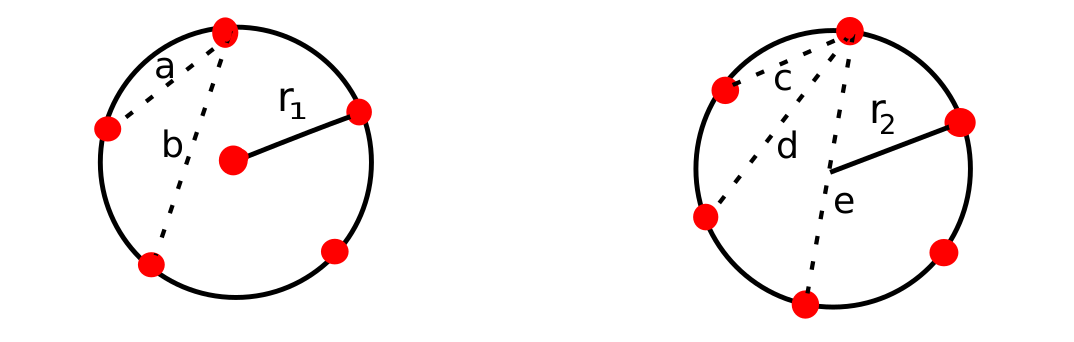
For this purpose we evaluate the internal potential energy (IPE) and the total potential energy (TPE) of the two possible configurations. Here the IPE is the amount of work done to bring the charges from infinite and make the cluster in the absence of an external electric field. TPE is the sum of IPE and parabolic potential energy due to external electric field. The schematic for (1,5) and (0,6) configurations is shown in Fig.1. The expression for IPE and TPE for the two configurations is written below:
| (2) |
| (3) |
where a, b, c, d, and e can be written in terms of and using relations
| (4) |
| (5) |
We have plotted the internal and total potential energy of both the configurations as a function of ring radius, as shown in fig.2. We find that in the absence of an external electric field, the IPE of both configurations does not have any minimum as expected. The configurations are not stable as charged particles repel each other. The external electric field tries to confine the particles giving rise to a minimum of total potential energy at a particular radius. This is shown in subplot (a) of Fig.2. Here the triangle(red) and square(green) denote the minimum of TPE for two possible configurations, viz., (1,5) and (0,6) respectively. In the presence of the external electric field, the value of TPE for the (1,5) configuration is less compared to that of (0,6) at the minima. This implies that the configuration (1,5) would be preferred over (0,6). The radius at which the minima of the TPE occurs is denoted by the red color triangle for which shown in Fig.2. This value matches precisely with the radius of the cluster observed in the relaxed state for simulations with particles. Thus formation of these configurations is based on the relaxation towards the minimum potential energy state.
The next question is related towards understanding those configurations which are unable to relax towards a stationary state. The characteristic feature exhibited by the dynamics in these cases is of further interest. These issues will now be adderssed in the next section.
IV Chaos in Dynamics
When the total number of the particle is such that they all get accommodated in a single radial shell or with one particle at a center and others on a single radial ring around it, the observed relaxed configuration is always stationary. For our simulations, this occurs till the total number of particles is in the system. When we increase the number of particles, the configurations become complex. They can be typically looked upon as structures for which particles are located on two or higher numbers of shells. For these cases, if the number of particles placed on each ring is integer multiple of each other, then the system relaxes towards a stationary state. If this condition is not satisfied, then the configuration displays complex dynamics. For instance, in clusters having 10 and 11 particles with configuration and respectively are shown in Table 1. For both these cases, the particles in the two shells are not related to each other by integer numbers. It is evident that for such combinations, there exists no possible placement of particles that can ever lead to a form for which the interparticle forces acting on every particle would be get balanced by the external force field, which would be required for a stationary configuration. A component of force, therefore, always remains unbalanced on some particles giving rise to interesting dynamics. We now try to understand the dynamics that are exhibited by such configurations. We have specifically chosen to illustrate this here with a detailed study of a configuration with particles. Other configurations exhibiting dynamical states have also been investigated, though they have not been presented here. The general inferences about the dynamics for all these cases remain similar.
We have shown the time evolution of the configuration of particles with two slightly different initial conditions in Fig.3. In subplots (a) and (c) we have shown the particle configuration at . It is to be noticed that the initial configurations of these two cases are slightly differ from each other. In subplot (b) and (d) the time evolution of these two configurations have been shown from to . Here, the color symbols from blue to red represent the increase of time. It is clear that the time evolution is drastically different even though the initial conditions were very close. The rotational dynamics observed is therefore sensitive to the chosen initial conditions.
We now track the angular velocity () of the particle defined by
| (6) |
here and are the and components of particle velocity and is the angle of rotation. In Fig.4 the time evolution has been shown for one of the particle located on the outer shells. Here, red (solid) and blue (dash) lines represents time evolution of for two different initial space distributions of particles shown in sub-plot (a) and (c) of Fig.3. The two plots of are almost identical to begin with and subsequently get uncorrelated. The vertical line in green at time separates the evolution which occurs before and after the cluster formation. It should be observed that the changing sign of corresponds to the changing direction of rotation. It should be observed from the figure that the time interval at which this occurs is fairly random.
Thus the system appears to be sensitive to a slight difference in the initial condition of the particles. We, therefore, analyze this system carefully quantitatively now.
IV.1 Time series analysis
In this section, we will mainly focus on the time history of for one of the particles, which has shown evidence of sensitivity towards initial conditions. In Fig.5 sub-plot (a) and (b) the Fourier transform and power spectrum of from to has been shown respectively. There are definite peaks in the frequency spectra against a noisy background. We can see from these subplots that the power spectrum is considerably broad, and there is no specific characteristic frequency of the system. The nature of the frequency and power spectrum is broad. The sub-plot (b) of Fig.5 shows that at the higher end of the spectrum, the power spectrum of falls as .
Identification of chaos in a series is a multistage process that includes calculating time delay coordinate, reconstructing phase space, calculating correlation dimension, and Lyapunov exponent Baker and Gollub (1996). The first step constitutes calculating the time-delay coordinate (). We want to reconstruct a phase space attractor, so it’s important to get a good estimate for the time delay () for this time series. The value of is a typical time after which one expects the correlation in the signal to die out. There are several methods by which we can calculate this time lag Fraser and Swinney (1986); Martinerie et al. (1992); Fraser (1989). It can thus be calculated by using either velocity autocorrelation or mutual information function. Fraser and Swinney Fraser and Swinney (1986) introduced an approach for selecting time delay using the first local minimum of mutual information function. Velocity auto-correlation examines the correlation in time series data as a function of time, and the first zero crossing gave an idea about . Here, we have a time-series of and its auto-correlation is shown in Fig.6. The first zero crossing corresponds to a delay of -time steps, which gives us time delay . Choosing this method would not introduce any bias as invariant quantities computing using reconstructed attractor are not very much sensitive to Baker and Gollub (1996).
The second step constitutes reconstruction of the phase space for this attractor, an abstract mathematical space spanned by the dynamical variable of the system. It was shown by Takens Takens (1981) that phase space can be reconstructed by time-delayed measurement of a single observed time-series signal. Fig.7 shows a reconstructed 3-D attractor for the time series of . In order to resolve the structure of the system in reconstructed phase space, the minimum embedding dimension is found to be using “False Nearest Neighbour” Kennel et al. (1992). For the choice of there were no self-intersections.
The third step is to calculate correlation dimension Grassberger and Procaccia (1983) . It should be independent of embedding dimension , which gives information about attractor that is effectively embedded in higher dimension space. We found that correlation dimension is . We observe that on changing the embedding dimension, the correlation dimension becomes independent of as shown in Fig.8. This suggests that the particle dynamics is not totally random but has chaotic attribute for which the attractor is strange with a non-integral dimension.
As the final step of our analysis, we try to find the Lyapunov exponent, which quantifies the mean divergence between neighboring trajectories in phase space for a chaotic system. The chaotic system must have at least one non-negative Lyapunov exponent. We evaluated the largest Lyapunov exponent (LLE) using the Rosenstein algorithm Rosenstein et al. (1993) by allocating the nearest neighbor on adjacent trajectories and computing the divergence between successive pairs along the trajectories. The slope of average logarithmic divergence is shown in subplot(a) of Fig.9 which gives the value of LLE as . The positive value of the LLE confirms that the system is chaotic.
We have carried out a similar analysis for other cluster configurations and observed that the rotational dynamics exhibited by the cluster configuration is essentially chaotic in nature. The Lyapunov index and other characteristics of the attractor for each case may, however, differ. For instance, in a cluster having particles the largest Lyapunov exponent is as shown in subplot (b) of Fig.9. The observation of strange attractors and positive LLE confirms the chaotic dynamics of particles inside the cluster.
We have also carried out Langevin dynamics simulation Feng et al. (2010) using LAMMPS Plimpton (1995), which includes the effect of neutral on dust particles of the cluster. The phase space trajectories in the attractor are a little distorted due to random kicks of neutrals with dust grains, but dynamics still remain chaotic with small changes in parameters like correlation dimension and Lyapunov exponent.
V Conclusion
Equilibrium and/or relaxed state for particles interacting with repulsive screened Coulomb/Yukawa potential in an overall radially confining force field was studied using Molecular Dynamics simulation. Such a system can be prepared easily in the laboratory by immersing charged micron-sized dust particles in ordinary electron-ion plasma. A biased ring electrode can provide the radial confinement. It is observed that the system relaxes towards a minimum energy configuration. In such a state, particles organize themselves in various shells around the center. Depending on the number of particles, the relaxed state is observed to be either stationary or exhibits a dynamical rotating state in which the particles arranged in various shells show rotation. The rotation changes with time, and detailed analysis shows that the dynamics is chaotic.
VI Acknowledgements
This research work has been supported by the J. C. Bose fellowship grant of AD (JCB/2017/000055) and the CRG/2018/000624 grant of DST. The authors thank IIT Delhi HPC facility for computational resources.
References
- Maity et al. (2020) S. Maity, P. Deshwal, M. Yadav, and A. Das, Physical Review E 102, 023213 (2020).
- Fan et al. (1992) S. Fan, S. Yang, J. Dai, S. Zheng, D. Yuan, and S. Tsai, Physics Letters A 164, 295 (1992).
- Mitra et al. (2014) V. Mitra, A. Sarma, M. Janaki, A. S. Iyenger, B. Sarma, N. Marwan, J. Kurths, P. K. Shaw, D. Saha, and S. Ghosh, Chaos, Solitons & Fractals 69, 285 (2014).
- Shaw et al. (2019) P. K. Shaw, N. Chaubey, S. Mukherjee, M. Janaki, and A. S. Iyengar, Physica A: Statistical Mechanics and its Applications 513, 126 (2019).
- Sheridan (2005) T. Sheridan, Physics of plasmas 12, 080701 (2005).
- Sheridan and Theisen (2010) T. Sheridan and W. Theisen, Physics of Plasmas 17, 013703 (2010).
- Juan et al. (1998) W.-T. Juan, Z.-H. Huang, J.-W. Hsu, Y.-J. Lai, and I. Lin, Physical Review E 58, R6947 (1998).
- Murillo (2004) M. S. Murillo, Physics of Plasmas 11, 2964 (2004).
- Chu and Lin (1994) J. Chu and I. Lin, Physical review letters 72, 4009 (1994).
- Thomas et al. (1994) H. Thomas, G. Morfill, V. Demmel, J. Goree, B. Feuerbacher, and D. Möhlmann, Physical Review Letters 73, 652 (1994).
- Hayashi and Tachibana (1994) Y. Hayashi and K. Tachibana, Jpn. J. Appl. Phys. 33, L804 (1994).
- Shukla and Mamun (2015) P. K. Shukla and A. Mamun, Introduction to dusty plasma physics (CRC press, 2015).
- Juan and Lin (1998) W.-T. Juan and I. Lin, Physical review letters 80, 3073 (1998).
- Teng et al. (2009) L.-W. Teng, M.-C. Chang, Y.-P. Tseng, and I. Lin, Physical review letters 103, 245005 (2009).
- Maity et al. (2018) S. Maity, A. Das, S. Kumar, and S. K. Tiwari, Physics of Plasmas 25, 043705 (2018).
- Melzer et al. (1996) A. Melzer, A. Homann, and A. Piel, Physical Review E 53, 2757 (1996).
- Schweigert et al. (1998) V. Schweigert, I. Schweigert, A. Melzer, A. Homann, and A. Piel, Physical review letters 80, 5345 (1998).
- Maity and Das (2019) S. Maity and A. Das, Physics of Plasmas 26, 023703 (2019).
- Plimpton (1995) S. Plimpton, Journal of computational physics 117, 1 (1995).
- Nosenko and Goree (2004) V. Nosenko and J. Goree, Physical review letters 93, 155004 (2004).
- Nosé (1984) S. Nosé, Molecular physics 52, 255 (1984).
- Hoover (1985) W. G. Hoover, Physical review A 31, 1695 (1985).
- Baker and Gollub (1996) G. L. Baker and J. P. Gollub, Chaotic dynamics: an introduction (Cambridge university press, 1996).
- Fraser and Swinney (1986) A. M. Fraser and H. L. Swinney, Physical review A 33, 1134 (1986).
- Martinerie et al. (1992) J. Martinerie, A. M. Albano, A. Mees, and P. Rapp, Physical Review A 45, 7058 (1992).
- Fraser (1989) A. M. Fraser, IEEE transactions on Information Theory 35, 245 (1989).
- Takens (1981) F. Takens, in Dynamical systems and turbulence, Warwick 1980 (Springer, 1981), pp. 366–381.
- Kennel et al. (1992) M. B. Kennel, R. Brown, and H. D. Abarbanel, Physical review A 45, 3403 (1992).
- Grassberger and Procaccia (1983) P. Grassberger and I. Procaccia, Physical review letters 50, 346 (1983).
- Rosenstein et al. (1993) M. T. Rosenstein, J. J. Collins, and C. J. De Luca, Physica D: Nonlinear Phenomena 65, 117 (1993).
- Feng et al. (2010) Y. Feng, J. Goree, and B. Liu, Physical Review E 82, 036403 (2010).