Technology, Institution, and Regional Growth: Evidence from Mineral Mining Industry in Industrializing Japan

Abstract

Coal extraction was an influential economic activity in interwar Japan. In the initial stage, coal mines used males and females as the miners worked in the pits. However, the innovation of labor-saving technologies and the renewal of traditional extraction methodology induced institutional change through the revision of labor regulations on female miners in the early 1930s. This dramatically changed the mines as the place where skilled males were the principal miners engaged in the underground works. I investigate the impact of coal mining on regional growth and assess how the institutional change induced by the labor regulations affected its process. By linking the location information of mines with registration- and census-based statistics, I found that coal mines led to remarkable population growth. The labor regulations did not stagnate but accelerated the local population growth as they forced female miners to exit from the labor market and form their families. The regulations prohibited risky underground works by female miners. This reduction in occupational hazards also improved early-life mortality via the mortality selection mechanism in utero.

Keywords: institution; mines; occupational hazard; regional economy; labor regulation; resource; structural shifts

JEL Codes: N30; N40; N50; N70; N90;

1 Introduction

How institution influences the economy has attracted wider attention (Hall and Jones 1999; Acemoglu et al. 2001). Institutional interventions in the labor market may impede development as they could prevent the labor market and structural adjustments (Freeman 1993; Fernández-Villaverde 2018). Cross-country evidence indicates that stronger regulation on labor markets could be associated with lower labor force participation and higher unemployment (Botero et al. 2004). Evidence based on the domestic variations in the labor regulation shows that pro-worker labor regulation decreases the economic activities in the formal manufacturing sector in India (Besley and Burgess 2004). However, a specific type of regulation, such as unemployment insurance, may improve risk-sharing and reduce the transaction cost in job search (Acemoglu and Shimer 1999). Therefore, understanding what labor regulations could hinder (or improve) economic performance is still an influential research agenda.

In this paper, I investigate how coal mining impacts the regional economic development in interwar Japan and how the institutional change concerning female labor patterns induced by the technology shocks influenced its process. In prewar Japan, the coal mining sector relied not only on male miners but also on female miners. However, the innovation of labor-saving technologies such as coal cutters and conveyors and the renewal of traditional extraction methodology induced institutional change through the revision of labor regulations on female miners in the interwar period. It dramatically changed the mining place from where female and male manual miners worked in the pits to where skilled male miners were the principal workers. Such an institutional change could have impacted the regional economy as it would increase the gender wage gap.

I found that the coal mine leads to population growth, indicating the regional development in the mining area. The revised labor regulations did not stagnate the local population growth but accelerated it because the institutional change due to the regulations had forced female miners to exit from the labor market and form their families. Since the revised regulation prohibited risky work in the pits by the female miners, it substantially reduced their occupational hazards. This led to the declines in overall female mortality and the improvements in the early-life mortality rates via the mortality selection mechanism in utero.

This paper adds to the literature on the role of the state and institutions during economic development from the perspective of female labor regulations (Botero et al. 2004; Besley and Burgess 2004). Importantly, it is the first study investigating the impacts of institutional change due to the regulations of female workers in the resource extraction sector. Coal is necessary for industrialization because broad economic activities heavily rely on coal consumption. I show that technology-induced labor regulations reduced female labor force participation and accelerated the local population growth through the family formation channel. This institutional change mitigated the occupational hazards for female miners and improved the early-life health status in the local economy. In this light, my findings shed new light on the role of gender-specific labor regulations in understanding the mechanisms behind regional economic growth.

This study is relevant to the broader literature on the economic impacts of resource extractions. Predictions regarding agglomeration theory imply that resource abundance can increase the demand for local labor in the mining sector and related industries, thereby causing an influx of population and agglomeration (Rosenthal and Strange 2004; Duranton and Puga 2004; Lederman and Maloney 2007). However, an increase in the resource extraction industry may stagnate the development of non-resource extraction industries by reallocating resources from the non-resource tradable sector (Sachs and Warner 1999, 2001). In fact, there are still debates on whether proximity to coal mines is necessary for regional economic growth during Europe’s industrialization. For example, a recent study by Fernihough and O’Rourke (2020) found that after the mid-eighteenth century, European cities closer to coalfields had a larger population than other cities. By contrast, Mokyr (1977) observed that the distribution of coal supplies did not contribute to industrialization.

My main results support the former assertion by showing that the coal mines led to population growth and structural shifts in the local economy. Importantly, this study adds to this literature to analyze the mechanism behind population growth due to resource extraction. Although studies have analyzed the impact of resource abundance on population growth, the mechanisms underlying this relationship have been understudied. I show that the population growth in the mining area initially occurred due to internal migration, but those people then formed families over time. Moreover, this study is the first to provide evidence that the institutional change induced by the technological shocks affected the impacts of the coal mines on the regional economy.

This paper also expands our understanding of the relationship between mining and regional human capital accumulation. A pivotal risk of mining is pollution, which can increase the health costs in resource-abundant locations and decrease agricultural productivity (Aragón and Rud 2015; von der Goltz and Barnwal 2019). To the best of my knowledge, however, the potential health risks of mining during historical industrialization have yet to be evaluated. I find that while there is little evidence on the air and water pollution pathways, occupational hazards for female miners lead to mortality selection in utero, which increases early-life mortality. Moreover, the regulations on female miners mitigated such mortality sorting mechanisms before births. My finding sheds light on the importance of occupational hazards in evaluating the economic activities of the resource extraction industry, which has been neglected in the literature. In addition, it provides suggestive evidence that labor regulations may improve the human capital of their offspring by improving early-life health conditions.

Finally, this study utilizes data on demographic, labor, and health outcomes constructed using census-based statistics. These data allow me to eliminate the risks caused by selection bias in the statistical inference. This study also has the advantage of exploiting specific geological strata given in nature as an instrumental variable, which offers robust estimates for evaluating the impacts of the coal mines on the regional economy. Moreover, this study provides the first evidence of a past-developing country in Asia, given that research has mainly focused on European countries, the US, Latin America, and African countries.

The remainder of the study is organized as follows. Section 2 briefly overviews the historical context. Section 3 summarizes the data. I describe the proposed identification strategy in Section 4. Section 5 presents the main results for the regional growth. Sections 6 and 7 provide the analyses on the regional health and labor supply, respectively. Section 8 overviews the robustness of the results, and Section 9 concludes.

2 Historical Background

2.1 Coal Mining Industry

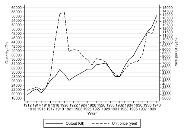
Figure 1: Coal Production in Japan from 1912 to 1940

Note: The solid line shows the coal output in giga tons (Gt). The dashed line indicates the coal price in yen per giga tons. The unit price is defined as the total price of coal output divided by the total coal output in each year.

Source: Created by the author. Data on coal output are from Ministry of International Trade and Industry (1954).

The Mining Code of 1892 allowed private companies to have mining concessions, accelerating the installation of modern technologies in mines and the development of Japan’s mining sector. For instance, winding engines were installed in the coal and copper mines in the 1890s, and the flame-smelting process was adopted in gold and silver mines in the 1900s (Ishii 1991, pp. 220–221). Before the First World War (WWI), the coal industry had developed as an export labor-intensive industry. However, WWI increased the average wage rates of miners, reducing the comparative advantage of the Japanese coal industry. Figure 1 illustrates the development of the coal industry and shows the negative shock in the early 1920s. This motivated coal mining firms to reduce the number of miners and adopt new extraction machines to improve firm productivity. Mining firms reallocate resources to relatively productive mines to improve their average productivity. Consequently, average labor productivity in the coal mining sector increased from the 1920s, particularly in the 1930s (Okazaki 2021). Figure 1 shows that total coal production increased during the interwar period.

In the early 1930s, coal accounted for approximately $55$% of total mineral output in Japan (Mining Bureau, Ministry of Commerce and Industry 1934, p.44). The large share of coal production indicates that coal extraction was an influential economic activity at that time. The higher wage rates of miners have motivated peasants to move into the extraction industry, shifting the local industrial structure from the primary to the production sector. For instance, the average daily wage of female miners working in the pits was one and a half to two times higher than those of the female workers in the silk and spinning industries (Nishinarita 1985, pp. 84–85). Besides the original inhabitants, therefore, mining workers would include a certain proportion of migrants. This may have influenced the structure of both the marriage market and fertility in the local economy surrounding mines. However, quantitative evidence of these changes in the regional economy is still lacking in literature.

2.2 Mining Technology, Occupational Hazards, and Regulations of Female Miners

By the end of the 19th century, a large part of mines had finished mechanizing the processes involved in hauling, such as drainage pumps and hoisting machines. However, this did not mean that the miner’s workload related to hauling operations was reduced. Instead, such mechanization in the main shafts had increased the workload of miners extracting and transporting coal around the face (Sumiya 1968, pp. 310–312).

In fact, the environment in the pit was generally poor. The air was polluted with dust, oxygen levels were low, and there was a risk of carbon monoxide poisoning. There was also a high fire risk from dynamite blasting and spontaneous combustion of gas and coal. Accidents caused by falling rocks occurred frequently. Available statistics indicate that the average number of accidents per year in the pits between 1917 and 1926, causing injuries and deaths of miners, was 142,595, of which 61,112 were from falling rocks. Accidents caused by explosions, poisoning, and suffocation were fewer than those caused by falling rocks, but they still occurred 311 times per year on average between 1917 and 1926 (Japan Mining Association 1928, p. table.6).

Notably, while miners included single male workers, a large proportion of them were married couples as miners usually worked in teams of two to three (Sumiya 1968, pp. 300–308). The male skilled miner, called saki yama, extracted coal at the face; meanwhile, the female miner, named ato yama, brought coal to the coal wagon at the gangway through steep pits using bamboo baskets called sura (Sumiya 1968, p. 319).

As coal is a bulky resource, the heavy work burden on pregnant women could have increased the risk of adverse pregnancy outcomes (Ahmed and Jaakkola 2007). Miners worked in pits with dirty air containing particulates, which eventually damaged their lungs and increased the risk of respiratory diseases such as tuberculosis (Sumiya 1968, pp.  410–411). Relatedly, a growing body of medical literature has revealed that particulates and radionuclides from coal increase the risk of stillbirths and premature deaths due to respiratory diseases in mothers (Landrigan et al. 2017; Lin et al. 2013).

An important event that changed such harsh labor pattern of female miners was an institutional change that occurred in the early 1930s. Following the International Labor Conference after World War I, the Social Affairs Bureau held a consultation meeting with miners in the 1920s to revise the Miners’ Labor Assistance Regulations of 1916. Initially, mining companies, who relied heavily on female miners for production, opposed the Social Affairs Bureau’s insistence on prohibiting women from working underground and late-night. However, the renewal of mining methods driven by new extraction technologies changed the attitudes of the mining companies in the late 1920s. In fact, the transition from the traditional room-and-pillar mining method to the longwall method was accompanied by the adoption of technologies such as coal cutters and conveyors.Compared to the room-and-pillar method, the coal extraction space of the longwall method is larger, allowing for the introduction of those machines (Nishinarita 1985, p. 91). Specifically, the conveyors could bring extracted coals from pits to gangway further efficiently than the female miners did, adding strong incentive to the mining companies to prohibit the underground works by the female miners (Tanaka and Ogino 1977, p. 79).At last, the Revised Miners’ Labor Assistance Regulations of September 1928 prohibited some underground and late-night work by female miners. Since the grace period for enforcement of the regulations lasted until 1933, the number of female miners gradually declined from around 1930. Table 1 shows that the number of female miners in the pits dropped from 1930 to 1933 when the revised regulation was enacted in September.

The full enforcement of the revised labor regulations did not eliminate female miners altogether because females were allowed to work in the pits of the thin layer and were primarily responsible for coal selection and other out-of-pit labor. More than 15,000 women still worked in the mines in the late 1930s, which represented approximately 10% of all the miners measured. Therefore, female miners played an essential role in the coal mines throughout the interwar period. However, it is also true that the technology-induced institutional change had substantially reduced the total number of female miners. This change further mitigated the occupational hazards for the female miners.

Table 1: Number of Coal Miners in the Manufacturing Censuses

	Female		Male		% share of
Year	Miners	Work in the pits (%)	Miners	Work in the pits (%)	female miners
1924	65147	$-$	179986	$-$	27
1927	56956	71	176524	76	24
1930	32680	60	153876	76	18
1933	15695	37	133460	77	11
1936	18694	25	178816	77	9

Notes: The statistics in this table are from the Labor Statistics Field Survey Reports that surveyed mines employing 50 or more miners. Figures in column 6 show the percentage share of females to the total number of miners.

Sources: Statistics are from Statistics Bureau of the Cabinet (1926, p. 5), Statistics Bureau of the Cabinet (1930, pp. 6–7), Statistics Bureau of the Cabinet (1932b, pp. 6–7), Statistics Bureau of the Cabinet (1936, p. 41), and Statistics Bureau of the Cabinet (1937, p. 45). The description of the survey subject is from Statistics Bureau of the Cabinet (1932a, p. 1) and Statistics Bureau of the Cabinet (1937, p. 1).

2.3 Mining Technology and Pollutions

Pollution may be another potential incidence that could influence the regional economy. Generally, industrial pollution was not recognized as a common social problem among the people of pre-war Japan. As a result, there is little documentation of pollution due to coal mining. Anecdotes, however, suggest that there are a few potential pathways that generate pollution around coal mines.

First was the soot and smoke caused by coal consumption to run steam-winding machines. Steam-winding engines were introduced early in the mechanization of the hauling process and exhausted the smoke from burning coal in the boiler. However, these steam-powered winders were gradually replaced with electric winders during the interwar period (Japan Mining Association 1930, 1931). Thus, this channel might be unlikely to impact the regional population health.

Second, presumably more relevant, is pollution from wastewater generated during mining. In the late 1930s, as coal mining became increasingly mechanized, some mines began introducing water-washing machines during coal sorting. Female miners who had worked in the pits before the prohibition of underground works in the early 1930s carried out this coal selection process. Unfortunately, there is little historical documentation systematically describing pollution caused by wastewater from coal mines. However, coal sludge from coal selection might have contaminated rivers to some extent at that time. An example is Onga river in the Chikuhō coalfield, which was called a “zenzai” (sweet red-bean soup), implying that the water was contaminated by the liquid waste (Chiba and Yamada 1964). Coal sludge contains several metal toxicities, including mercury (Hg) and cadmium (Cd), which are known to be associated with the incidence of miscarriages and stillbirths (Amadi et al. 2017; Sergeant et al. 2022). This suggests the possibility that the early-life mortality would have been higher in the coal mining region with greater river accessibility.

Overall, mining may influence the regional economy in several aspects. Firstly, the increased demand for local labor in the mining sector should lead to an influx of population. This must initially disturb the local demographic trends in the mining area. Secondly, occupational hazards and/or pollution could have impacted the regional population health. The heavy workloads and poor environments in the pits must have increased the risks of entire and early-life mortality. Environmental pollution may also increase the risks. Finally, the institutional change due to the revision of labor regulations may impact the regional economy because it substantially reduced the number of female miners and the gender wage gap in the local labor market.

3 Data

This study created a unique dataset of demographic outcomes, labor supply, and early life health outcomes across mining areas in the Japanese archipelago. Because mining is a localized economic activity, a smaller lattice dataset is preferred to identify the impact of mines. I collected and digitized a set of official census-based municipal-level statistics published in the 1930s.

3.1 Mine Deposit

I use official reports named Zenkoku kōjyō kōzan meibo (lists of factories and mines) published by Association for Harmonious Cooperation (1932, 1937) (hereafter, called the AHC), which document coal mine locations measured in October 1931 and October 1936. The AHC listed all mines with $50$ miners and more, meaning that very small-scale mines with fewer than $50$ mimers are outside this study’s scope. Thus, the main target of this study is the average impact of small- to large-scale coal mines and not the very small-scale collieries. This does not discount the comprehensiveness of the AHC because it still includes information on small-scale mines, which have been neglected in the literature.

I define the treatment group as the municipalities located within 0–5 km of the centroid of a municipality with mines. A 5 km threshold is fundamentally plausible because the mean value of the distance to the nearest neighborhood municipality is approximately 4 km. In fact, the estimated effects disappeared in the statistical sense outside the 5 km range, which means that the potential spillover effect is captured under this threshold. Finer details of the validity of this threshold are summarized in Online Appendix C.4. For the control group, I set the threshold as 5–30 km from the centroid.

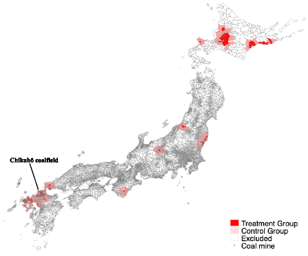
(a) 1931

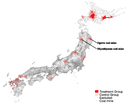
(b) 1936

Figure 2: Spatial Distribution of the Treated and Controlled Municipalities

Notes: The white circles indicate the location of municipalities with coal mines. The treatment (control) group highlighted in red (pink) includes the municipalities within 5 (between 5 and 30) km from a mine. The excluded municipalities are shown as empty lattices in the figures.

Source: Created by the author.

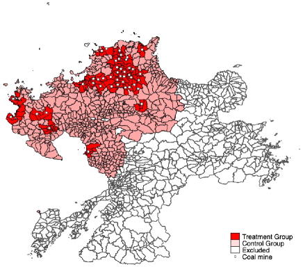
(a) 1931

(b) 1936

Figure 3: Location of Coal Mines around Chikuhō Coalfield in Kyushū

Notes: 1. The white circles indicate the location of municipalities with coal mines around Chikuhō coalfield (Figure 2a) in Kyushū region. Figure 3a shows the coal mines in Chikuhō, Kasuya, and Miike coalfields in Fukuoka, Karatsu coalfield in Saga, and Miike coalfield in Kumamoto. Amakusa coalfield in Kumamoto is added in Figure 3b (on the lower left of the figure). Ōita prefecture does not have coal mines but is shown in the figures to explain the border of the sample.

2. Treatment (control) group includes municipalities within 5 (between 5 and 30) km from a mine. The excluded municipalities are shown as empty lattices in the figures.

Source: Created by the author.

Figure 2 indicates the coal mine locations from the AHC and the corresponding treatment and control groups by year. Most coal mines are located in three specific areas in the southernmost, central, and northeastern regions: these are representative coalfields called Chikuhō, Jyōban, and Ishikari-Kushiro Tanden, respectively. Notably, a comparison of Figures 2a and 2b shows that these agglomerations were stable over time. For a closer look, Figure 3 provides an example map for a representative coalfield called Chikuhō-tanden in Kyushū island, Japan’s southernmost region (indicated in Figure 2a). One can see that the distribution of mines has changed little; only a few mines were opened or closed between 1931 and 1936. This feature of coal mines makes it difficult to use within-variation in the spatial distribution of the mines for identification. Online Appendix C.7 discusses this point in detail.

Finally, I explain the creation of the analytical samples. From $11,151$ total municipalities, I first retain the municipalities within a $30$ km radius from the centroid of the municipalities with mines. I then exclude the intersection of the different types of mines, such as municipalities within $5$ km from a gold, silver, and copper (GSC) mine. Table B.3 presents the summary statistics of the treatment variables. The number of municipalities in the analytical sample based on the 1931 and 1936 AHC were $1,140$ and $1,364$, respectively. Meanwhile, the proportion of treated municipalities was approximately $15$% and $13$%, respectively, for each sample.

3.2 Geological Stratum

The spatial distribution of a specific geological stratum created in the Cenozoic era, which includes some carboniferous ages, is used as an instrumental variable (IV) for the location of coal mines (Section 4). Data on the geological strata are obtained from the official database of the Ministry of Land, Infrastructure, Transport and Tourism, which includes roughly nine thousand stratum points. I matched each municipality in my analytical sample with the nearest stratum point to identify the municipalities with the relevant stratum. Online Appendix B.2 provides finer details of the IV’s definition and an example of a geological columnar section of a representative coal mine to show the relevance of the IV. Table B.3 presents the summary statistics of the indicator variables for the stratum.

3.3 Outcomes

Demographics

The primary dependent variable, population, is obtained by digitizing the municipal-level statistics documented in the 1930 and 1935 Population Censuses (Statistics Bureau of the Cabinet 1935b, 1939). To investigate the mechanism behind the potential local population growth due to mining, I also digitized the Municipal Vital Statistics of 1930 and 1935 (Statistics Bureau of the Cabinet 1932c, 1938), which document the total number of marriages, live births, and deaths in all municipalities in the survey years. I then consider four dependent variables: sex ratio, average household size, crude marriage rate, crude birth rate, and crude death rate by gender. These demographic variables represent the characteristics of marriage markets and family formation in the local economy. Using these variables, I assess whether the local population growth due to mining activity depended on immigrants and/or changes in the family planning of local people. Importantly, as the census documents the total number of people in all municipalities in the census years, it helps us avoid sample selection issues. Table B.4 presents the summary statistics of the demographic outcomes by treatment status and census year. The mean differences are statistically significant for most variables, implying that systematic demographic changes may have occurred around the mining extraction area.

Early-life Health

Next, I examine the infant mortality rate (IMR) to assess the impacts on early-life health. To analyze the potential mechanisms behind the shifts in infant mortality, I use the fetal death rate (FDR). To obtain both variables, I digitized the 1933 and 1938 reports documenting municipal-level statistics on births and infant deaths published by the Aiikukai and Social Welfare Bureau. I also consider the mortality rate of children aged 1–4 to assess the potential impacts of air pollution. All these statistics are based on official vital statistics. An important advantage of using these vital statistics is that since Japan has a comprehensive registration system, the data cover almost all fetal and infant death incidences in the measured years. Table B.4 shows the summary statistics of the early life health variables. Again, the mean differences were statistically significant.

Labor Supply

I consider the labor force participation rate, the number of workers per $100$ people, to investigate the impacts on local labor supplies. To analyze structural shifts, the employment share of workers in the mining, agricultural, manufacturing, commercial, and domestic sectors are considered; these are calculated as the number of workers in each industry per $100$ workers. I use the labor force participation rates of both sexes to better understand the potential gender bias among the changes in local labor markets. These labor statistics were obtained from the prefectural part of the 1930 Population Census. Panel C of Table B.4 presents the summary statistics of these variables by treatment status and census year. Similar to the demographic outcomes, the mean differences are statistically significant for most variables, which implies the potential impact of mining extraction.

3.4 Additional Control Variables

Accessibility to Railway Stations

As coal is a bulky mineral, railways were used to transport the extracted coal. Firms may have preferred setting extraction points closer to railway stations to reduce transportation costs (Sumiya 1968, pp. 440–441). Further, the local population size could be larger if one moves closer to stations. Therefore, controlling for the distance between each municipality and the nearest-neighboring station is preferable to deal with this potential endogeneity issue. I used the location information of all stations obtained from the official dataset provided by the Ministry of Land, Infrastructure, Transport and Tourism to compute the nearest-neighbor distance to stations in 1931 and 1936. Online Appendix B.4 summarizes the details of the data, and Online Appendix Figure B.5 shows the locations of these stations across the Japanese archipelago. Table B.5 shows the summary statistics.

Accessibility to Sea Ports

Although railways were primarily used to transport coal because coal mines were usually inland (Online Appendix Figure 2), marine transportation was also used for secondary logistics. Hence, similar to railway transportation, I include the distance to the nearest neighboring seaport as a variable to control for accessibility to marine transportation (Online Appendix Figure B.6 shows seaport locations). Online Appendix B.5 summarizes the data details and Table B.5 shows the summary statistics.

Accessibility to Rivers

Finally, I consider the accessibility to rivers. Not all mining areas have large rivers suitable for water transportation (Online Appendix Figure B.7). This means that rivers did not dominate the locations of coal mines. However, several mines used river transport as primary logistics until the development of railways before the late 1920s (Chiba and Yamada 1964). This implies that the spatial distribution of the river might have influenced the location of mines in such mining areas. Thus, I included the distance to the nearest neighboring river as a control variable. Online Appendix B.6 describes the details of the data, and Table B.5 shows the summary statistics. I also used the river accessibility variable to test the potential pollution from wastewater (Section 6).

4 Identification Strategy

I leverage the random nature of mineral deposits to identify the effects of mines. The linear regression model is as follows:

$$\footnotesize{\begin{split}y_{i}=\alpha+\beta\text{{MineDeposit}}_{i}+\mathbf{x}_{i}^{\prime}\bm{\gamma}+e_{i},\end{split}}$$ (1)

where $i$ indexes municipalities, $y$ is the outcome variable, MineDeposit is an indicator variable that equals one for municipalities within 5 km from a mine, $\mathbf{x}$ is a vector of control variables, and $e$ is a random error term.

Because the placement of a mine is determined by a geological anomaly, MineDeposit is random in nature (Benshaul-Tolonen 2019, p.1568). However, the rest of the variation may be correlated with the local variation in infrastructure. For instance, if a mineral deposit is found between a village and a city, the mining firm may choose the city as its main mining point because the city is likely to have better infrastructure than the village. Then, MineDeposit can be positively correlated with the error term, leading to a positive (negative) omitted variable bias in the estimate of $\beta$ if the placement of the city is positively (negatively) correlated with the outcome variable. To deal with this systematic bias in the ordinary least squares, I included two indicator variables that equal one for cities and towns, respectively. As explained in Section 3.4, I also include the distances to the nearest neighboring railway station, seaport, and river to control for transportation accessibility. The differences in the estimates from both specifications, including and excluding the control variables, indicate how much this omitted variable mechanism influences the results. Thus, I can partially assess the randomness of the primary exposure variable (MineDeposit). As I show later, the results from the simple regressions are materially similar to those from the specifications, including the control variables, thereby supporting the randomness of the exposure variable. To be conservative, I prefer the specification including the control variables (equation 1).

A potential threat in the identification may be measurement errors in time-dimensional assignments. As explained in Section 3.1, mine data were surveyed in October 1931 (1936), whereas the Population Census was conducted in October 1930 (1935). Similarly, data on fetal death and infant mortality were obtained from the 1933 (1938) Vital Statistics. The lags in the matching allow me to consider the exposure durations. For instance, fetus miscarriages in 1933 (1938) were in utero conceived in 1932 (1937), whereas their mothers should have been exposed to any shocks at the time of conception in 1932 (1937). The same argument can be applied to infant mortality: infants who passed away in 1933 (1938) were born at the beginning of 1932 (1937) at the earliest. Therefore, they should have been in utero in 1931 (1936). Consequently, the mining data that list the mines in October 1931 and 1936 may be reasonably matched with the health data of 1933 and 1938, respectively. However, one must be careful as there is still a one-year lag in matching with both the census and vital statistics datasets. This may lead to attenuation bias due to miss assignments in the time dimension, because the number of coal mines should be increased during that year.

To deal with such potential issues, I consider the IV estimator using the exogenous variation in the geological stratum. In this IV approach, Equation  1 is regarded as a structural form equation because the least-squares estimator ($\hat{\beta}$) is assumed to be attenuated by the measurement error in the exposure variable.

The reduced-form equation for MineDeposit is designed as follows:

$$\footnotesize{\begin{split}\textit{MineDeposit}_{i}=\kappa+\tau\textit{Stratum}_{i}+\mathbf{x}^{\prime}_{i}\bm{\mu}+\epsilon_{i},\end{split}}$$ (2)

where Stratum is a binary IV that equals one for municipalities with sedimentary rock created during the Cenozoic era, and $\epsilon$ is a random error term. The IV is plausibly excluded from the structural equation because the location of mines is essentially dominated by the distribution of geological stratum, which is exogenously given in nature and unobservable by people in the prewar period. In addition, the relevance condition holds because the location of coalfields is determined by the distribution of the stratum created in the Cenozoic era, which includes the Carboniferous period when the strata containing coal were created (Fernihough and O’Rourke 2020). Online Appendix B.2 summarizes the geological strata variable in finer detail and shows that the location of coal mines is determined by specific strata created in the Cenozoic era. Online Appendix C.2 discusses the validity of identification assumptions in more rigorous way.

I use the heteroskedasticity-consistent covariance matrix estimator as a baseline estimator. For the sensitivity check, I also use the standard errors clustered at the county level based on the cluster-robust covariance matrix estimator (Arellano 1987) to determine the influence of the potential influences of the local-scale spatial correlations. Online Appendix C.3 shows that the results are materially similar under both variance estimators. Therefore, the potential spatial correlations were negligible in this empirical setting.

5 Regional Development: Evidence from the Population Censuses

Table 2: Coal Mining and Regional Development:
Local Population Growth in the Mining Area

Panel A: 1930 Census
	Dependent Variable: ln(Population)
	(1)	(2)	(3)	(4)
MineDeposit	$1.386***$	$0.829***$	$0.812***$	$0.447***$
	$(0.291)$	$(0.197)$	$(0.211)$	$(0.058)$
City and Town FEs	No	Yes	Yes	Yes
Railway accessibility	No	No	Yes	Yes
Port accessibility	No	No	Yes	Yes
River accessibility	No	No	Yes	Yes
Observations	1,140	1,140	1,140	1,140
Estimator	IV/Wald	IV	IV	OLS
First-stage $F$-statistic	$43.39$	$37.70$	$32.19$	$--$
Mean of the DV	$8.29$	$8.29$	$8.29$	$8.29$
Panel B: 1935 Census
	Dependent Variable: ln(Population)
	(1)	(2)	(3)	(4)
MineDeposit	$1.401***$	$0.870***$	$0.895***$	$0.457***$
	$(0.278)$	$(0.188)$	$(0.194)$	$(0.057)$
City and Town FEs	No	Yes	Yes	Yes
Railway accessibility	No	No	Yes	Yes
Port accessibility	No	No	Yes	Yes
River accessibility	No	No	Yes	Yes
Observations	1,364	1,364	1,364	1,364
Estimator	IV/Wald	IV	IV	OLS
First-stage $F$-statistic	$48.87$	$44.11$	$40.48$	$--$
Mean of the DV	$8.27$	$8.27$	$8.27$	$8.27$

***, **, and * represent statistical significance at the 1%, 5%, and 10% levels, respectively. Standard errors based on the heteroskedasticity-robust covariance matrix estimator are reported in parentheses.

Notes: Panels A and B show the results for the 1930 and 1935 samples, respectively. The mean (standard deviation) of the log-transformed population for the 1930 and 1935 samples are 8.29(0.74) and 8.27(0.74), respectively. Panel A of Table B.4 shows the summary statistics for the population (before log-transformed).

Panel A of Table 2 presents the main results for the population in 1930. The estimate from a simple IV estimation is shown in column 1. Then I include the city and town fixed effects (column 2) and both the fixed effects and control variables (column 3). The estimated coefficient decreases from $1.386$ to $0.829$ when I include the fixed effects. This suggests that, as expected, the location of the coal mines may be positively correlated with the local infrastructure. Including additional control variables on transportation accessibility has little influence on the estimate ($0.812$), supporting the evidence that, after conditioning on the fixed effects, there are no influential unobservables that are potentially correlated with the location of mines. Panel B confirms the similar results for the population in 1935 in the same column layouts. The estimated coefficient from the specification including the full set of controls in column (3) is $0.895$, which is larger than that for the 1930 sample.

The estimated magnitude is economically meaningful. The estimates from the preferred specification of column (3) indicate that coal mines increased the local population by $125$% in 1930 (panel A) and $145$% in 1935 (panel B). The average number of miners per coal mine increased just less than $100$ during this period ($1,567$ in 1931 and $1,658$ in 1936). In this light, it is a bit surprising that the magnitude is estimated to be much greater in the 1935 sample. I will assess a potential explanation behind this trend in the next mechanism analysis section.

In column 4, I present the estimates based on the reduced-form assumption to see if the IV approach works as expected. Even after conditioning on the control variables, the estimates based on the IV approach in column (3) are greater than those in column (4). This implies that my IV estimation strategy dealt with the systematic attenuation due to the measurement errors.

5.1 Assessing the Mechanisms

My results from each cross-sectional sample imply that municipalities with coal mines in the 1930s experienced local population growth. A natural question is whether it results from natural increase or labor migration. Given that the flow data on the migrants is unavailable, I try to infer this mechanism using the available censuses and vital statistics.

Following the geometric population growth model, I hypothesize the population dynamics in the coal mining area within a very short-run, from time $t$ to $t+1$, can be specified as follows:

$$\footnotesize{\begin{split}\Psi_{t+1}-\Psi_{t}=\Pi_{t}+\Upsilon_{t}-\Omega_{t},\end{split}}$$ (3)

where $\Psi$, $\Pi$, $\Upsilon$, and $\Omega$ indicate the number of people, net migrants, live births, and deaths, respectively. The main scope herein is to analyze how the coal mines impacted each factor (i.e., migration, fertility, and mortality) before and after 1933, when the revision of regulations was fully enacted.

As explained, the number of net migrants is unobservable. Thus, I test this channel using the sex ratio and the average household size measured in the population censuses. If labor migrations were the leading cause, municipalities with mines should have had a disproportionate (i.e., higher) sex ratio and smaller household sizes because new miners were usually single males and couples. On the other hand, the natural growth channel is testable using the births and deaths statistics comprehensively measured in the vital statistics. In short, if the population grows naturally from family planning, municipalities with mines should have had higher marriage and fertility rates, and lower mortality rates.

First, I conducted my cross-sectional analysis using the IV estimation strategy to assess each pathway. I then compare the magnitudes for different years to discuss the potential mechanism behind the growth of the estimated magnitude of the coal mines on the local population. Table 3 presents the results. All the regressions include the fixed effects as well as the control variables.

5.1.1 During the Grace Period of the Revision of Regulations

Table 3: Testing the Mechanisms: Migration of Male Miners, Family Formation and Fertility,
and Improvements in Female Mortality

	1930 Census
	Migration		Family Formation		Mortality
Panel A	(1) Sex Ratio	(2) HH Size	(3) Marriage	(4) Fertility	(5) Male	(6) Female
MineDeposit	$0.115***$	$-0.438***$	$-2.585***$	$-7.020***$	$0.254$	$-1.852$
	$(0.036)$	$(0.145)$	$(0.825)$	$(2.055)$	$(1.517)$	$(1.459)$
City and Town FEs	Yes	Yes	Yes	Yes	Yes	Yes
Railway accessibility	Yes	Yes	Yes	Yes	Yes	Yes
Port accessibility	Yes	Yes	Yes	Yes	Yes	Yes
River accessibility	Yes	Yes	Yes	Yes	Yes	Yes
Observations	1,140	1,140	1,140	1,140	1,140	1,140
Estimator	IV	IV	IV	IV	IV	IV
First-stage $F$-statistic	$32.19$	$32.19$	$32.19$	$32.19$	$32.19$	$32.19$
Mean of the DV	$0.99$	$5.34$	$8.59$	$34.06$	$20.06$	$18.59$
	1935 Census
	Migration		Family Formation		Mortality
Panel B	(1) Sex Ratio	(2) HH Size	(3) Marriage	(4) Fertility	(5) Male	(6) Female
MineDeposit	$0.050**$	$-0.284**$	$-1.387**$	$-1.144$	$-1.182$	$-2.857**$
	$(0.024)$	$(0.128)$	$(0.677)$	$(1.576)$	$(1.201)$	$(1.142)$
City and Town FEs	Yes	Yes	Yes	Yes	Yes	Yes
Railway accessibility	Yes	Yes	Yes	Yes	Yes	Yes
Port accessibility	Yes	Yes	Yes	Yes	Yes	Yes
River accessibility	Yes	Yes	Yes	Yes	Yes	Yes
Observations	1,364	1,364	1,364	1,364	1,364	1,364
Estimator	IV	IV	IV	IV	IV	IV
First-stage $F$-statistic	$40.48$	$40.48$	$40.48$	$40.48$	$40.48$	$40.48$
Mean of the DV	$0.99$	$5.34$	$9.04$	$34.22$	$18.36$	$16.97$

***, **, and * represent statistical significance at the 1%, 5%, and 10% levels, respectively. Standard errors based on the heteroskedasticity-robust covariance matrix estimator are reported in parentheses.

Notes: 1. Panels A and B show the results for the 1930 and 1935 samples, respectively.

2. “Sex Ratio”, “HH Size”, “Marriage”, “Fertility”, “Male”, and “Female” indicate the sex ratio (male/female), average household size, crude marriage rate, crude birth rate, male death rate, and female death rate, respectively (Panel A of Online Appendix Table B.4).

3. The mean (standard deviation) of the sex ratio and average household size in 1930 and 1935 samples are 0.99 (0.08) and 5.34 (0.47), and 0.99 (0.07) and 5.34 (0.57), respectively. The mean (standard deviation) of the crude marriage rate and crude birth rate in the 1930 and 1935 samples are 8.59 (2.28) and 34.06 (5.52), and 9.04 (2.41) and 34.22 (5.47), respectively. The mean (standard deviation) of the male death rate and female death rate in the 1930 and 1935 samples are 20.06 (4.48) and 18.59 (4.33), and 18.36 (4.12) and 16.97 (4.21), respectively.

Panel A presents the results for the 1930 sample. The estimated coefficients in columns 1 and 2 indicate that municipalities with coal mines experienced an increase in the sex ratio and a decline in the household size. The estimated magnitudes are economically meaningful. Both estimates ($0.12$ and $0.44$) account for roughly one standard deviation in the sex ratio and the average household size (Panel A in Online Appendix Table B.4). This implies that the influx of single males had distorted the sex ratio and had decreased the average number of household members in the mining area. Although the result tells only about the single male immigrants, the married couple miners shall also have immigrated given the labor pattern in the coal mines (Section 2).

In columns 3–4, I test the fertility channel using the crude marriage and birth rates. The estimates for the rates are negative and statistically significant. Both estimates ($-2.59$ and $-7.02$) are greater than one standard deviation of each dependent variable, suggesting economically meaningful effects. This result makes sense because the influx of single male miners could be associated with lower marriage and fertility among the entire local population.

Columns 5–6 summarize the results for the mortality channel by gender, showing that the estimates are close to zero and statistically insignificant.

Taken together, the coal mines increased the net migration but decreased the fertility rate, suggesting the conditions of $\Pi>0$, $\Upsilon<0$, and $\Omega\approx 0$ in equation 3. This implies that the population growth in the mining area was mainly led by the influx of population in the early 1930s, which is basically consistent with implication from the agglomeration theory.

5.1.2 After the Full Enforcement of the Revision of Regulations

Panel B of Table 3 presents the results for the 1935 sample. The coal mining area changed after fully enacting the revised labor regulations.

In columns 1–2, the estimated magnitudes for the sex ratio and average household size ($0.05$ and $0.28$) are much smaller than those for the 1930 sample. Relatedly, columns 3–4 provide evidence that both marriage and fertility rates had been reverting to those natural trends. The estimated coefficients are much smaller in an absolute sense ($-1.39$ and $-1.14$), and the estimate for the fertility rate is no longer statistically significant. Columns 5–6 show that the estimate for the female death rate turns out to be statistically significant, whereas that for the male death rate is still close to zero and statistically insignificant. The estimated magnitude of female mortality increased from $-1.85$ in 1930 to $-2.86$ in 1935. The latter accounts for roughly $0.8$ standard deviation of the female mortality in 1935, which is not negligible.

These results are consistent with the historical facts in the following two aspects.

First, the revision of the regulations decreased the number of female miners, as discussed in Section 2. This institutional change has liberated women from dangerous underground work, which may have improved the health status of females. However, given the gender wage gap, it also pushed them out of the local labor market and shifted them to domestic work. Section 7 shows the evidence on this structural shift for female workers. This may have forced women to take on the role of building a family. The increase in fertility means reversing the overall sex ratio because the sex ratio at birth shall have a regular gender balance at that time. It follows that the average household size increased.

Second, as mechanization progressed, miners were required to accumulate knowledge and experience in operating machinery. Management, therefore, had an incentive to encourage miners to form families and continue employment over a long term (Morimoto 2013). For example, many coal mines were equipped with nurseries and other welfare facilities from the 1920s (Ministry of Commerce and Industry 1926). My results obtained seem to be in line with this attitude of companies.

To summarize, I find evidence that the miners had begun to form their families in the mid-1930s given the labor regulations on the female miners. This suggests the conditions of $\Upsilon>0$ and $\Omega<0$ in equation 3. Table 1 confirms that the total amount of miners had been relatively stable or even slightly increased between 1930 and 1935, supporting that net migration was still positive ($\Pi>0$). Taken together, a plausible explanation for the greater marginal effect on the local population in the mid-1930s is a change in the sign of the natural growth term ($\Upsilon-\Omega$) from negative to positive by the local family formation due to the institutional change in the early 1930s.

6 Occupational Hazards for Female Miners: Evidence from the Vital Statistics

I have documented the regional growth in the coal mining area and provided evidence that the revision of regulations had influenced the trends in the demographics. In this section, by using the early-life mortality measured in the registration-based vital statistics, I assess to what extent the occupational hazards influenced the reproductive health of female miners and whether the institutional change improved such hazards. I also consider the potential channel due to the mining pollution.

My results suggest that although the occupational hazards had decreased the health status of fetuses and infants, the institutional change had mitigated those risks. There is little evidence that the air and water pollution due to mining led to higher early-life mortality.

6.1 Theoretical Framework: Mortality Selection before Birth

First, I illustrate a theoretical framework for mortality selection in utero to better interpret the quantitative evidence from the vital statistics data. The biological sorting mechanism in utero suggested by the Trivers-Willard hypothesis (TWH) (Trivers and Willard 1973) implies that there are two possible cases in which fetuses are exposed to health shocks: scarring and selection.

Let $x\sim\mathcal{N}(\mu,\,\sigma^{2})$ be the initial health endowment of the fetus in utero, and assume that there is a survival threshold $x_{s}$ below which the fetus is culled before birth. First, the scarring mechanism shifts the mean of the distribution ($\mu$) toward the left as $\mu^{*}<\mu$, such that $x^{*}\sim\mathcal{N}(\mu^{*},\,\sigma^{2})$. As the survival threshold $x_{s}$ is fixed, this shift implies that the number of culled fetuses must increase as $F^{*}(x_{s})>F(x_{s})$, where $F^{*}(\cdot)$ and $F(\cdot)$ indicate the cumulative distribution functions (CDF) of the normal distributions with means $\mu^{*}$ and $\mu$, respectively. Similarly, the conditional expectation of the initial health endowment at birth satisfies the following condition:

$$\footnotesize{\begin{split}E[x^{*}|x^{*}>x_{s}]<E[x|x>x_{s}].\end{split}}$$ (4)

This means that the health endowment of surviving infants is more likely to decline due to fetal health shocks.

Contrarily, the selection mechanism shifts the survival threshold ($x_{s}$) toward the right as $x_{s}^{*}>x_{s}$. As the mean of the distribution is fixed, this shift also increases the number of culled fetuses as $F(x_{s}^{*})>F(x_{s})$. Consequently, the conditional expectation of endowment at birth satisfies the following condition:

$$\footnotesize{\begin{split}E[x|x>x_{s}]<E[x|x>x_{s}^{*}].\end{split}}$$ (5)

This implies that the health endowment of surviving infants is more likely to be improved if the selection mechanism works.

The propositions can be summarized as follows. First, fetal health shocks may increase the risk of fetal death through both mechanisms. Second, the risk of infant mortality increases (decreases) in the scarring (selection) mechanism. Third, if both mechanisms work simultaneously, the risk of infant mortality remains unchanged. Considering these, I use the fetal death and infant mortality rates to test whether coal mines had adverse health effects and which mechanism worked in the case of mineral mining exposure.

6.2 Scarring due to the Occupational Hazards

Table 4: Institutional Change Mitigated the Occupational Hazards for Female Miners

Panel A: 1933 Vital Statistics
	Analytical Sample
	Full		Treated		Full	Treated
	(1) IMR	(2) FDR	(3) FDR	(4) IMR	(5) CMR	(6) CMR
MineDeposit	$36.912**$	$22.921**$			$-0.108$
	$(16.976)$	$(10.146)$			$(2.905)$
Female Miner			$0.034**$	$0.098**$		$0.004$
			$(0.013)$	$(0.034)$		$(0.004)$
Male Miner			$-0.002$	$-0.007*$		$-0.001$
			$(0.002)$	$(0.004)$		$(0.001)$
River accessibility	$-1.283$	$-0.393$	$-1.343$	$-0.552$	$-0.244*$	$0.168$
	$(0.933)$	$(0.537)$	$(1.842)$	$(2.466)$	$(0.135)$	$(0.318)$
City and Town FEs	Yes	Yes	Yes	Yes	Yes	Yes
Railway accessibility	Yes	Yes	Yes	Yes	Yes	Yes
Port accessibility	Yes	Yes	Yes	Yes	Yes	Yes
Observations	1,140	1,140	93	93	1,140	93
Estimator	IV	IV	OLS	OLS	IV	OLS
First-stage $F$-statistic	$32.19$	$32.19$	$--$	$--$	$31.19$	$--$
Mean of the DV	$117.15$	$43.51$	$53.90$	$147.19$	$13.40$	$16.06$
Panel B: 1938 Vital Statistics
	Analytical Sample
	Full		Treated		Full	Treated
	(1) IMR	(2) FDR	(3) FDR	(4) IMR	(5) CMR	(6) CMR
MineDeposit	$17.411$	$6.680$			$1.417$
	$(12.420)$	$(8.236)$			$(2.558)$
Female Miner			$0.025*$	$0.066**$		$0.005$
			$(0.015)$	$(0.030)$		$(0.004)$
Male Miner			$0.001$	$0.000$		$0.000$
			$(0.001)$	$(0.002)$		$(0.000)$
River accessibility	$-1.162*$	$-0.379$	$0.186$	$-0.922$	$-0.286*$	$-0.285$
	$(0.646)$	$(0.475)$	$(1.588)$	$(1.655)$	$(0.152)$	$(0.395)$
City and Town FEs	Yes	Yes	Yes	Yes	Yes	Yes
Railway accessibility	Yes	Yes	Yes	Yes	Yes	Yes
Port accessibility	Yes	Yes	Yes	Yes	Yes	Yes
Observations	1,364	1,364	115	115	1,364	115
Estimator	IV	IV	OLS	OLS	IV	OLS
First-stage $F$-statistic	$40.48$	$40.48$	$--$	$--$	$40.48$	$--$
Mean of the DV	$114.33$	$37.30$	$50.16$	$135.91$	$16.81$	$20.70$

***, **, and * represent statistical significance at the 1%, 5%, and 10% levels, respectively. Standard errors based on the heteroskedasticity-robust covariance matrix estimator are reported in parentheses.

Notes: Panels A and B show the results for the 1933 and 1938 Vital Statistics samples, respectively (Panel B of Table B.4). Columns 1–2 show the results for the entire sample. Columns 3–4 show the results for the municipalities with coal mines (i.e., the municipalities included in the treatment group). Columns 5–6 show the results for the full sample and the municipalities with coal mines, respectively. The IMR, FDR, and CDR indicate the infant, fetal, and child mortality rates, respectively (Panel B of Table B.4). The mean (standard deviation) of the IMR, FDR, and CDR in the 1933 sample is 117.15 (42.66), 43.51 (27.41), and 13.40 (9.58), respectively. Those in the 1938 sample are 114.33 (42.79), 37.30 (25.68), and 16.81 (8.73), respectively.

Panel A of Table 4 presents the results for the 1933 sample. Column 1 shows that the estimate for the IMR is positive and statistically significant, indicating that coal mines increased the infant mortality risk. In column 2, I run the same regression by replacing the IMR with FDR to assess the mechanism behind the higher risk of infant mortality in coal mining areas. The estimate is positive and statistically significant. This implies that the greater risk was associated with reducing fetal health endowments by mining, supporting evidence on the scarring mechanism before birth (Section 6.1).

Next, I test whether the occupational hazard led to this scarring due to coal mining. In column 3, I limited my sample to $93$ municipalities with coal mines to analyze the correlation between the FDR and the number of female miners and accessibility to rivers. If heavy manual work during pregnancy affects fetal health, FDRs should be positively correlated with the number of female miners. To control for the scale effect and provide a placebo test, I included the number of male workers simultaneously in the same specification. The estimated coefficient for female miners is significantly positive, whereas that for male miners is rather negative. This result supports the evidence that occupational hazards for females (not males) alone increased the risk of death before birth. The estimate indicates that a one standard deviation increase in female miners ($=269.2$ miners) increases the number of fetal deaths by roughly $9$ ($0.034\times 269$) per 1000 births. This is economically meaningful because the mean difference in the FDR between the treatment and control groups was also approximately $9$ fetal deaths per 1000 births (Panel B of Online Appendix Table B.4). Column 4 shows the result for the IMR, showing that the estimated coefficient on the number of female miners is also statistically significantly positive. It further provides evidence that this reduction in fetal health endowment via occupational hazards for females is associated with higher infant mortality risks.

Panel B of Table 4 provides the results for the 1938 sample in the same panel and column layout. Columns 1–2 show positive but much smaller estimates, which are no longer statistically significant. The estimates listed in columns 3–4 are also positive, but smaller in magnitude. The estimate for the FDR shows that a one standard deviation increase in female miners ($=179.3$ miners) increased the number of fetal deaths by approximately $4.5$ ($0.025\times 179$) per 1000 births. This magnitude was less than half of that in 1933.

The decline in the estimated magnitude of these health outcomes between 1933 and 1938 could partly be associated with an improving trend in health-related risk-coping strategies, such as increments in the number of medical doctors and installation of modern water supply (Online Appendix Figure C.5). However, the city and town fixed effects as well as accessibility variables control for the heterogeneities in such local sanitary levels.

Taken together, my results imply that the occupational hazards had increased the early-life mortality risk through the scarring mechanism in utero. However, the risks had been substantially decreased in the late 1930s because the full enforcement of the revised labor regulations changed the labor patterns of female miners and furthermore reduced the number of female miners. Therefore, the institutional change may have attenuated the mortality selection mechanism before births throughout the 1930s.

Testing the Pollutions

Section 2 suggests that the coal sludge generated from the coal selection process might have been a potential pollution factor. Suppose such wastewater increases the health risk of fetuses and infants. In that case, municipalities with mines closer to rivers should have significantly higher mortality rates because the wastewater had been discharged into the rivers (Chiba and Yamada 1964). However, the estimated coefficients of the river accessibility variable are close to zero and statistically insignificant in columns 1 and 2 in Panel A, and this does not largely change in Panel B. This result suggests that, although wastewater was occurring as anecdotes suggest, it was not enough to harm the health conditions of mothers and infants.

Moreover, air pollution is also unlikely to increase mortality risks. If air pollution increases the early-life mortality, then the estimated coefficients on the male miner should be positive in columns 3 and 4 because larger mines should emit more coal smoke from the boilers of the steam winding machines. As shown, however, the estimates are very close to zero in all the cases. Column 5 of Panel A further tests the potential influence of air pollution using an alternative outcome, the mortality rate of children aged 1–4. If air pollution mattered, the child mortality rate should be greater in the coal mining area than in the surrounding regions because younger children are more susceptible to pollutants because they are more likely to play outside than infants. The estimate is, however, close to zero and is statistically insignificant. Column 6 of Panel A uses data on $93$ municipalities with coal mines and provides further evidence on this: the estimated coefficients on the number of female and male miners are very close to zero, suggesting that child mortality did not depend on the scale of emissions. The results for child mortality in 1938 are similar to those in 1933 (columns 5–6 in Panel B).

Overall, air pollution does not seem to be a plausible channel to explain the greater early-life mortality in the mining area. This is consistent with the historical fact that winding machines were electrified in the interwar periods (Section 2).

7 Gender-Biased Structure Shift: Evidence from the 1930 Census

Table 5: Institutional Change Resulted in the Gender-Biased Structural Shift

Panel A: Male Workers
	Dependent Variable
		Employment Share
	(1) LFPR	(2) Mining	(3) Agricultural	(4) Manufacturing	(5) Commerce	(6) Domestic
MineDeposit	$-0.696$	$34.451***$	$-35.136***$	$1.753$	$-1.914$	$-0.439***$
	$(1.167)$	$(5.076)$	$(6.539)$	$(2.192)$	$(1.577)$	$(0.139)$
City and Town FEs	Yes	Yes	Yes	Yes	Yes	Yes
Railway accessibility	Yes	Yes	Yes	Yes	Yes	Yes
Port accessibility	Yes	Yes	Yes	Yes	Yes	Yes
River accessibility	Yes	Yes	Yes	Yes	Yes	Yes
Observations	1,140	1,140	1,140	1,140	1,140	1,140
Estimator	IV	IV	IV	IV	IV	IV
Mean of the DV	$57.13$	$3.16$	$60.39$	$13.91$	$7.86$	$0.37$
Panel B: Female Workers
	Dependent Variable
		Employment Share
	(1) LFPR	(2) Mining	(3) Agricultural	(4) Manufacturing	(5) Commerce	(6) Domestic
MineDeposit	$-18.930***$	$24.342***$	$-25.144***$	$-9.727***$	$3.057$	$4.731***$
	$(4.214)$	$(4.162)$	$(5.964)$	$(2.210)$	$(2.666)$	$(1.434)$
City and Town FEs	Yes	Yes	Yes	Yes	Yes	Yes
Railway accessibility	Yes	Yes	Yes	Yes	Yes	Yes
Port accessibility	Yes	Yes	Yes	Yes	Yes	Yes
River accessibility	Yes	Yes	Yes	Yes	Yes	Yes
Observations	1,140	1,140	1,140	1,140	1,140	1,140
Estimator	IV	IV	IV	IV	IV	IV
First-stage $F$-statistic	$33.57$	$33.57$	$33.57$	$33.57$	$33.57$	$33.57$
Mean of the DV	$40.77$	$1.83$	$74.03$	$5.93$	$10.11$	$4.21$

***, **, and * represent statistical significance at the 1%, 5%, and 10% levels, respectively. Standard errors based on the heteroskedasticity-robust covariance matrix estimator are reported in parentheses.

Notes: Panels A and B show the results for male and female worker samples, respectively, from the 1930 Population Census (Panel C of Table B.4). Column (1) shows the results for the labor force participation rates (%), whereas Columns (2)–(6) show the results for employment share in each industrial sector (%). The mean (standard deviation) of the labor force participation rates, and the employment share in each industrial sector in the male sample are 57.13 (3.30), 3.16 (10.09) for mining, 60.39 (23.62) for agriculture, 13.91 (8.04) for manufacturing, 7.86 (6.44) for commercial, and 0.37 (0.54) for the domestic sector, respectively. Those for the female sample are 40.77 (10.65), 1.83 (6.92), 74.03 (21.90), 5.93 (8.78), 10.11 (10.10), and 4.21 (3.93), respectively.

In this section, I aim to evaluate how the coal mines influence the local industrial structure using labor supply statistics from the 1930 population census. Theory predicts the positive correlation between the resource extractions and local labor supply. Allcott and Keniston (2018) provides evidence of such a relationship for the oil and gas extraction industries in the post-World War II U.S. economy. My results show that the impacts of the coal mine on local labor supply depended on gender. While the local labor supply for male workers was not influenced by the coal extractions, that for female workers decreased with a meaningful magnitude. The rapid mechanization and institutional change observed in interwar Japan, which is not considered in the case of the postwar U.S. economy, may explain the gap in the findings. The labor-saving technological advances might had reduced the labor required in the mining sector and the labor regulations had further displaced women from the sector.

Male Workers

Panel A of Table 5 presents the results for the male workers. Column 1 shows the estimate for the male LFP is very close to zero and statistically insignificant. This indicates that coal mines did not influence the labor supply of male workers in the local economy.

Columns 2–6 show the results for the employment share of male workers. Column 2 indicates that coal mines increased the mining sector’s employment share by approximately 34%, leading to a similar decline in the agricultural sector’s employment share (column 3). This suggests that the structural shift in male workers’ employment occurred mainly in the agricultural sector. In column 4, the estimate for the manufacturing sector is positive, suggesting a marginal spillover effect of mines on the manufacturing industry in the mining areas. However, this effect is not statistically significant. Compared with the case of the 1970s U.S., the rapid mechanization may not have created the time window for generating spillover effects in the case of interwar Japan. The estimates for the commercial and domestic sectors are moderately negative and close to zero (columns 5–6, respectively). This is consistent with male workers being less likely to work in these service sectors (Panel C of Online Appendix Table B.4).

Female Workers

The results for female labor listed in Panel B show different responses. Column 1 shows a statistically significantly negative estimate, providing evidence that the coal mines decreased the female LFP. The estimate suggests that coal mines decreased the female LFP rate by approximately $19$%. This may be partly explained by the fact that the sample period is in the grace period of the revision of the regulations.

Columns 2–6 show the results for the employment share of female workers. Column 2 indicates that coal mines increase the mining sector’s employment share by $24$% and decrease the agricultural sector’s share by the same degree (column 3). The estimated magnitude is smaller than that for male workers (Panel A). This makes sense because, on average, females were less likely to work in mines than males (Table 1). While the manufacturing sector’s employment share decreases in the mining area (column 3), the estimates for the commercial and domestic sectors are moderately positive (columns 5–6, respectively). This is consistent with the increased relative demand for personal services from mining workers in mining areas (Caselli and Coleman II 2001).

Overall, I show clear gender differences in the local labor supply in the coal mining area. Males were engaged in mining work, whereas females were more likely to work in the domestic service industry or even exited from the labor markets, given the labor regulations. In this light, coal mining had led to gender-biased structural shifts in the case of 1930s Japan.

8 Robustness

I ensure the robustness of my results in the following ways. First, I used the cluster-robust variance-covariance matrix estimator in Online Appendix C.3. The results are robust to the potential influences of the local-scale spatial correlations. Second, I consider the potential influence of the altitude in the models because terrain may be associated with the local climatic conditions and fixed cost of transportation. The results are not sensitive to including the average altitude created using the grid cell data. Online Appendices B.7 and C.5 summarize the grid cell data and results, respectively. Third, I consider the regional heterogeneity in the endowment of male miners. The coal mines in Hokkaidō (northernmost island) were less likely to use female miners in the pits, given the nature of the labor supply of male miners. My results are materially similar if I include an indicator variable for Hokkaidō prefecture in the regressions (Online Appendix C.6). Fourth, I employ an alternative identification strategy. As explained in the data section, the nature of the assignments makes it difficult to employ the estimation strategy utilizing within variations of each unit. Nevertheless, I provide a case study using the DID approach for the subsample of the Tohoku region (northeastern region). The results are reasonable to the findings from my main results (Online Appendix C.7). Finally, I assess the validity of my results on coal mines by comparing the results for heavy metal mines. Since coal mining requires many more workers than heavy metal mining because coal is a bulky mineral, the estimated magnitudes for the heavy metal mines shall be much smaller. I confirm that the results are reasonable to such expectation (Online Appendix C.8).

9 Conclusion

The innovation of labor-saving technologies had occurred with the renewal of traditional extraction methodology in the coal mining sector in interwar Japan. These technology shocks induced the revision of labor regulations on the female miners, which led to institutional change concerning the females’ local labor market in the coal mining area. In this study, I examine the impact of coal mines on the regional economy during historical industrialization in interwar Japan and investigate how the institutional change influenced the effect.

To avoid potential selection bias, I utilize data on demographics, early-life health, and labor outcomes constructed using a set of official census-based statistics. I exploit the exogenous variation from the geological stratum to structurally identify the impacts of the coal mines on the regional economy. Several robustness checks confirm that my main results are not sensitive to the potential confounding factors and influential observations and the use of alternative variation in the estimation.

I find that the coal mines increased the local population, and its magnitude is greater in the sample after the full enforcement of the revised labor regulations. Evidence from the analyses using the local demographics and labor supply indicates that the regulations may have forced female miners to exit from labor market and to form their families. Before the full enforcement of the regulation, the occupational hazards for female miners substantially increased the early-life mortality via the biological mortality selection mechanism in utero. This institutional change, however, further led to improvements in early-life mortality.

The literature on institutional interventions in the labor market has provided evidence that labor regulations can impede regional developments as they can reduce the local labor supply and increase the unemployment (Botero et al. 2004). The revised labor regulations reduced the female labor supply and led to the gender-biased structural shift in the case of interwar Japan. My main findings, however, show that technology-induced labor regulations accelerated the local population growth through the family formation channel. In this process, the regulations played a role in mitigating the occupational hazards for female miners and improving the early-life health status in the local economy. I show the role of institutional change from the gender-specific labor regulations in understanding the mechanisms behind regional economic growth.

Appendices

Appendix Appendix A Background Appendix

A.1 Female Miners in Coal Mine

By the end of the 19th century, many mines in the Chikuhō coal fields had finished mechanizing the processes involved in hauling, such as drainage pumps and hoisting machines. However, this did not mean that the miner’s workload related to hauling operations was reduced. Instead, such mechanization in the main shafts had increased the workload of miners extracting and transporting coal around the face (Sumiya 1968, pp.  310–312).

Figure A.1a shows a photo of miners at the mine face (kiriha) in the 1910s. A male skilled miner (saki-yama) extracted coal, whereas a female miner (ato-yama) brought the coal using a bamboo basket called sura. Figure A.1b shows that ato-yama tied a rope around her body to prevent the heavy sura from slipping off in the steep pits. The environment in the pit was generally poor. The air was polluted with dust, oxygen levels were low, and there was a risk of carbon monoxide poisoning. There was also a high fire risk from dynamite blasting and spontaneous combustion of gas and coal. Moreover, accidents caused by falling rocks occurred frequently..

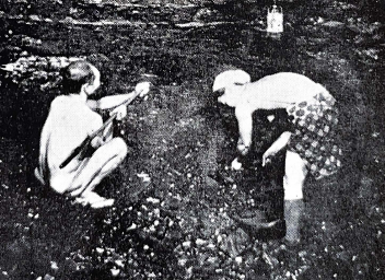
(a) Saki-yama (left) and Ato-yama (right)

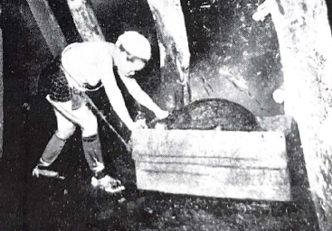
(b) Ato-yama using Sura

Figure A.1: Male (saki-yama) and Female Miners (ato-yama)

Notes: Figure A.1a shows the skilled male miner (saki-yama) extracting coal and the female miner (ato-yama) supporting her husband at the face. Figure A.1b illustrates an ato-yama bringing coal using a bamboo basket (sura) at the gangway through the steep pits. Both figures were taken in the early Taishō period.

Source: Fumoto (1961, p. 2).

The introduction of new mining technologies, such as coal cutters, was gradually adopted in the 1920s. The introduction of these technologies was accompanied by a transition from the traditional room-and-pillar mining method to the longwall method, which is more suitable for mechanical coal extraction. The number of miners, both male and female, declined during this transition. However, this did not entirely change the labor patterns of female miners. Approximately one in five miners was a woman in 1930 (Table 1), and they still worked inside the pits as ato-yama.

A significant event that changed the labor pattern of female miners was an institutional change that occurred in the early 1930s. Following the International Labor Conference after World War I, the Social Affairs Bureau held a consultation meeting with miners in the 1920s to revise the Miners’ Labor Assistance Regulations of 1916. Mining companies, who relied heavily on female miners for production, opposed the Social Affairs Bureau’s insistence on prohibiting women from working underground and late-night, but the Revised Miners’ Labor Assistance Regulations of September 1928 prohibited some underground and late-night work. Since the grace period for enforcement of the regulations lasted until 1933, the number of female miners gradually declined from around 1930. Table 1 shows that the number of female miners in the pits (ato-yama) dropped from 1930 to 1933, when the Revised Miner’s Labor Assistance Regulations were enacted in September. Mining companies responded to this decline by introducing coal conveyors (Tanaka and Oghino 1977, p. 79). Importantly, however, the revised regulations did not eliminate female miners altogether. Female miners were allowed to work in the pits of the thin layer and were primarily responsible for coal selection and other out-of-pit labor. More than 15,000 women still worked in the mines in the late 1930s, which represented approximately 10% of all the miners measured.

A.2 Influence of Great Depression in Japan

The impact of the Great Depression was not substantial in Japan compared to that in other countries (Miyamoto 2008, pp.  56–57; Abe 2008, p. 106; Blumenthal 1981, pp. 46). Blumenthal (1981, p.43) shows that the index of industrial production in Japan did not decrease dramatically between 1929 (=100) and 1930 (=97). In contrast, the US and the UK suffered much more significant reductions (81 in the US and 92 in the UK) in the same period. Blumenthal (1981, p. 45) also reports that the unemployment rates between 1930 and 1935 in the US, the UK, and Japan were approximately 27%, 15%, and 6%, respectively. Consequently, Japan’s GNP growth rate (from 1929 to 1930) was positive at $1.1$%, whereas it was $-7.7$ and $-0.1$, respectively, in the US and UK. This evidence supports the validity of using the systematic data from the census and vital statistics of the 1930s.

A.3 Shares of Coal and GSC Mines

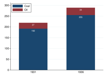
(a) Coal and oil mines

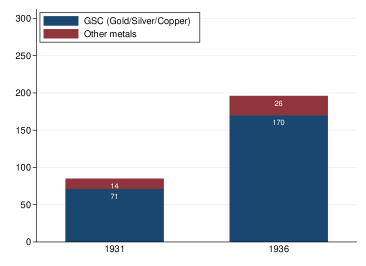
(b) Metal mines

Figure A.2: The Number of Coal, Oil, GSC, and the Other Metal Mines
in 1931 and 1936

Notes: This figure shows the number of coal and oil (Figure A.2a) and metal mines (Figure A.2b) documented in the AHCs of 1931 and 1936. GSC indicates gold, silver, and copper mines.

Source: Created by the author. Data on mines are from the Association for Harmonious Cooperation (1932, 1937).

Figure A.2a shows the number of coal and oil mines documented in the AHCs in 1931 and 1936. Similarly, Figure A.2b shows the numbers of GSC and other metal mines. As shown, approximately 90 (85)% of mines extracting fuels (metals) were coal (GSC) mines. Figure A.2 shows the number of mines, not municipalities. Since several mines coexist in a municipality, the number of municipalities with mines reported in the main text is smaller than the number of mines.

Appendix Appendix B Data Appendix

B.1 Mine Deposit

Data on the location and type of mines are obtained from the official reports published by the Association for Harmonious Cooperation (1932, 1937). They document all mines with more than $50$ miners in October 1931 and October 1936. The documents list three types of mines: metal, coal, and oil. In these documents, the mine’s location is indicated by the name of the municipality. Hence, the name of the municipality was used while geocoding to match the mine dataset with the datasets of the other variables. The shapefile used for geocoding was obtained from the official database of the Ministry of Land, Infrastructure, Transport and Tourism (available at: https://nlftp.mlit.go.jp/ksj/gml/datalist/KsjTmplt-N03-v2˙2.html (accessed on 23rd February 2021). Several municipalities were consolidated between the years 1930 and 1938. Thus, I used the municipality boundaries defined in 1938 and aggregate statistics for consolidated municipalities. A minimal number of municipalities were divided; these were excluded from the original dataset. To check all consolidations and divisions of municipalities, I used Zenkoku shichōsonmei hensen sōran (Municipal Autonomy Research Association 2006), the most comprehensive book on the history of municipalities’ names.

The initial dataset included both coal and heavy metal mines. To prepare the analytical samples, therefore, I had to exclude the duplications to identify the impacts of coal mines better. Panel A of Table B.1 summarizes duplications in the coal mine sample. Columns (1) and (2) show the figures based on the 1931 (1936) AHC, which is used to match with the 1930 (1935) Population Census and 1933 (1938) Vital Statistics datasets. Initially, there are $11,151$ municipalities in columns (1) and (2); note that the municipality boundaries are defined based on the 1938 boundaries. The number of municipalities within 30km of a coal mine is $1,147$ and $1,386$ in columns (1) and (2), respectively. The number of duplications in the treatment groups based on the $5$ km radius definition is $0$ and $2$ in columns (1) and (2), respectively. Similarly, the number of duplications in the control groups based on the $5$ km radius definition is $7$ and $20$ in columns (1) and (2), respectively. Following the trimming step shown in Figure B.1a, the analytical coal mine samples are $1,140$ ($=1,147-7$) and 1,364 ($=1,386-22$), respectively. Panel B of Table B.1 summarizes the duplications in the GSC mine sample. Following the same procedure as in Figure B.1b, the GSC mine samples used in the robustness analysis are $2,498$ ($=2,510-22$) and $3,293$ ($=3,337-44$), respectively.

The red (blue) circles in Figure B.2 indicate the coal (GSC) mine locations from the AHC. Figure 2 illustrates the spatial distribution of the coal mine sample by year and group. Figure 3 shows the distribution in Chikuhō coalfield in Kyushū in detail.

Table B.1: Duplications between Coal and GSC Mines

	(1)1930 or 1933	(2)1935 or 1938
Panel A: Coal mine sample
Number of total municipalities	11,151	11,151
Number of municipalities within 30km from a coal mine	1,147	1,386
Duplications in treatment group
Number of municipalities with a coal mine	93	115
of which has a GCS mine	0	1
Number of municipalities within 5km from a coal mine	167	179
of which has a GCS mine within 5km	0	2
Duplications in control group
Number of municipalities with no coal mines	1,054	1,335
of which has a GCS mine	3	12
Number of municipalities with no coal mines within 5km	980	1,271
of which has a GCS mine within 5km	7	20
Panel B: GSC mine sample
Number of total municipalities	11,151	11,151
Number of municipalities within 30km from a coal mine	2,510	3,337
Duplications in treatment group
Number of municipalities with a GSC mine	67	111
of which has a coal mine	0	1
Number of municipalities within 5km from a coal mine	125	174
of which has a coal mine within 5km	0	2
Duplications in control group
Number of municipalities with no GSC mines	2,437	3,196
of which has a coal mine	6	29
Number of municipalities with no GCS mines within 5km	2,373	3,119
of which has a coal mine within 5km	12	42

Source: See Online Appendix B.1.

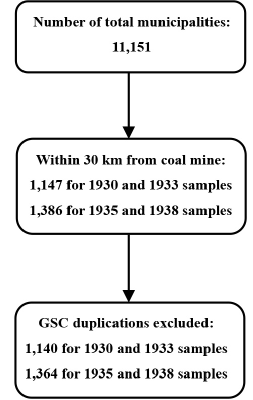
(a) Coal

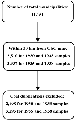
(b) GSC

Figure B.1: Construction of Analytical Samples

Notes: These figures show how to trim the municipalities into the analytical samples. Figures B.1a and B.1b show the trimming steps for the coal and GSC (gold, silver, and copper) mines, respectively.

Sources: Created by the author.

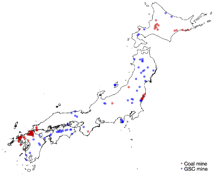
(a) 1931

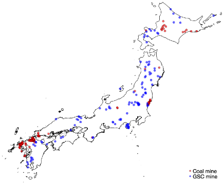
(b) 1936

Figure B.2: Location of Coal and GSC mines in 1931 and 1936

Notes: The red and blue circles indicate the locations of coal and GSC (gold, silver, and copper) mines, respectively. Chikuhō coalfield in Fukuoka prefecture in Kyushū region is indicated with an arrow in Figure B.2a. Figure 3 illustrates the coal mines around Chikuhō coalfield in detail.

Source: Created by the author.

B.2 Geological Stratum

I used the location information on geological strata (chisō) obtained from the official database of the Ministry of Land, Infrastructure, Transport and Tourism (available at: http://nrb-www.mlit.go.jp/kokjo/inspect/landclassification/download/index.html, accessed on 27th February 2020). The instrumental variable (IV) was defined as follows: First, I matched each municipality with the nearest stratum point ($11,151$ municipalities with $8,748$ stratum points). Figure B.3 illustrates the spatial distributions of the geological stratum and the mine locations (shown as circles). The average distance from the municipality’s centroid to the nearest stratum point was approximately 4 km (median = 3 km). This is shorter than the main treatment indicator variable of 5 km as the threshold for treatment. Second, using the analytical sample (Section 3.1), I regressed the indicator variable for coal mines on the strata to determine a plausible stratum strongly correlated with the location of coal mines. The data on the strata included 19 types of strata (with four categories of rock (and field) and six categories of era). I ran 19 regressions for each year’s (1931 and 1936) coal mine sample on the location of coal mines. Table B.2 presents the results. As shown, two strata, Tn and Tp, have statistically significant and positive correlations with the location of mines. Among them, the estimated coefficient for Tp has the most significant value ($0.323$ versus $0.143$ in the 1931 sample).

Tn and Tp are sedimentary rocks created during the Cenozoic era (shinseidai). Tp was created during a much earlier period, called the Paleogene period (ko daisanki), compared to Tn, which was made during the Neogene period (shin daisanki). Evidence indicates that Tp includes some coal layers created in the carboniferous ages (Nagao 1975). Figure B.4 shows a geological columnar section of the Iizuka coal mine, a representative coal mine in the Chikuho coalfield.

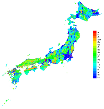
Figure B.3: Spatial distribution of mines and geological strata

Note: The white circles indicate the location of the mines. The strata are illustrated through colors.

Sources: Created by the author. Data on the location of mines are obtained from the Association for Harmonious Cooperation (1932, 1937). Data on the geological stratum are obtained from the Ministry of Land, Infrastructure, Transport and Tourism.

Table B.2: Defining Instrumental Variables for the Coal Mine Subsample

	Mining points in 1931			Mining points in 1936
Stratum	Coeff.	Std. Err.	$R$-squared	Coeff.	Std. Err.	$R$-squared
Sedimentary rock
M	$0.060$	$(0.073)$	$0.001$	$0.025$	$(0.051)$	$0.000$
P	$0.036$	$(0.122)$	$0.000$	$-0.034$	$(0.055)$	$0.000$
Pls	$0.020$	$(0.167)$	$0.000$	$0.037$	$(0.167)$	$0.000$
Tn	$0.143***$	$(0.040)$	$0.017$	$0.193***$	$(0.042)$	$0.028$
Tp	$0.323***$	$(0.049)$	$0.071$	$0.336***$	$(0.047)$	$0.074$
al	$-0.038$	$(0.031)$	$0.001$	$-0.033$	$(0.025)$	$0.001$
ds	$-0.147***$	$(0.011)$	$0.001$	$-0.131***$	$(0.009)$	$0.001$
lm	$0.020$	$(0.167)$	$0.000$	$-0.072$	$(0.060)$	$0.001$
tr	$-0.106***$	$(0.020)$	$0.015$	$-0.075***$	$(0.019)$	$0.008$
wf	$-0.123***$	$(0.030)$	$0.004$	$-0.109***$	$(0.026)$	$0.003$
Metamorphic rock
Gn	$-0.147***$	$(0.011)$	$0.000$	$-0.132***$	$(0.009)$	$0.002$
Sch	$-0.011$	$(0.046)$	$0.000$	$-0.007$	$(0.042)$	$0.000$
Body of water
w	$-0.147***$	$(0.011)$	$0.001$	$-0.131***$	$(0.009)$	$0.001$
Igneous rock
An	$-0.108***$	$(0.025)$	$0.007$	$-0.107***$	$(0.020)$	$0.007$
Bs	$-0.031$	$(0.051)$	$0.000$	$-0.027$	$(0.046)$	$0.000$
Gd	$0.133$	$(0.051)$	$0.002$	$0.122$	$(0.112)$	$0.002$
Gr	$-0.059**$	$(0.025)$	$0.004$	$-0.058***$	$(0.021)$	$0.004$
Lp	$-0.150***$	$(0.011)$	$0.004$	$-0.134***$	$(0.009)$	$0.005$
Sp	$0.054$	$(0.200)$	$0.000$	$0.013$	$(0.143)$	$0.000$

***, **, and * represent statistical significance at the 1%, 5%, and 10% levels, respectively. Standard errors based on the heteroskedasticity-robust covariance matrix estimator (Horn et al. 1975) are reported in parentheses.

Notes: The number of observations for 1931 and 1936 are $1,140$ and $1,364$, respectively.

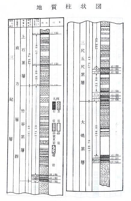
Figure B.4: Geological Columnar Section of the Iizuka Coal Mine

Note: This geological columnar section shows the strata around the Iizuka coal mine, including coal layers. The first to third columns include the names of layers created in the Paleogene period. The fourth to seventh columns examine the length of each layer, columnar, and legend. The black layers shown in the columnar of the sixth column are the coal layers: more than ten coal layers are included in the layers created in the Paleogene period.

Source: Fumoto (1961, p. Chishitsu chūjyō zu).

Table B.3: Summary Statistics: Mine and Instrumental Variables

	Year	Coal mines			GSC mines
		Mean	Std. Dev.	Obs.	Mean	Std. Dev.	Obs.
Mine Deposit	1931	$0.146$	$0.354$	$1140$	$0.050$	$0.218$	$2498$
	1936	$0.130$	$0.336$	$1364$	$0.053$	$0.224$	$3293$
Stratum	(1931)	$0.094$	$0.292$	$1140$	$--$	$--$	$--$
	(1936)	$0.086$	$0.280$	$1364$	$--$	$--$	$--$
Female Miners	1931	$207.51$	$269.16$	$93$	$51.91$	$71.13$	$57$
	1936	$145.65$	$179.77$	$115$	$40.73$	$59.18$	$111$
Male Miners	1931	$1359.25$	$1710.20$	$93$	$511.86$	$784.73$	$57$
	1936	$1512.84$	$2040.87$	$115$	$451.01$	$680.58$	$111$

Notes: This table shows the summary statistics for the indicator variable for the treatment group, geological stratum, and number of miners. The treatment (control) group is 0–5 (5-30) km from the centroid of a municipality that has a mine. The geological stratum is a time constant variable: “Year” in parenthesis indicates the matched year. GSC mines indicate gold, silver, and copper mines.

Sources: Data on the location of mines are from the Association for Harmonious Cooperation (1932, 1937).

B.3 Outcomes

Table B.4: Summary Statistics: Outcome Variables

Panel A:	Year	Overall			Treated			Controlled
Demographics		Mean	Std. Dev.	Obs.	Mean	Std. Dev.	Obs.	Mean	Std. Dev.	Obs.
Population	1930$\ddagger$	$6305.06$	$14829.74$	$1140$	$13091.93$	$25577.78$	$167$	$5140.20$	$11692.06$	$973$
	1935$\ddagger$	$6202.12$	$15598.06$	$1364$	$12986.87$	$28001.89$	$177$	$5190.41$	$12464.17$	$1187$
Sex ratio (male/female)	1930$\ddagger$	$0.99$	$0.08$	$1140$	$1.03$	$0.10$	$167$	$0.98$	$0.07$	$973$
	1935$\ddagger$	$0.99$	$0.07$	$1364$	$1.03$	$0.08$	$177$	$0.98$	$0.07$	$1187$
Household size	1930$\ddagger$	$5.34$	$0.47$	$1140$	$5.18$	$0.41$	$167$	$5.37$	$0.47$	$973$
	1935$\ddagger$	$5.34$	$0.57$	$1364$	$5.20$	$0.44$	$178$	$5.36$	$0.59$	$1187$
Crude marriage rate	1930$\ddagger$	$8.59$	$2.28$	$1140$	$7.43$	$2.19$	$167$	$8.79$	$2.24$	$973$
	1935$\ddagger$	$9.04$	$2.41$	$1364$	$7.98$	$2.05$	$177$	$9.20$	$2.42$	$1187$
Crude birth rate	1930$\ddagger$	$34.06$	$5.52$	$1140$	$31.75$	$5.62$	$167$	$34.46$	$5.40$	$973$
	1935$\ddagger$	$34.22$	$5.47$	$1364$	$32.37$	$4.96$	$177$	$34.50$	$5.49$	$1187$
Crude death rate (male)	1930	$20.06$	$4.48$	$1140$	$20.04$	$4.62$	$167$	$20.06$	$4.45$	$973$
	1935	$18.36$	$4.12$	$1364$	$177$	$17.90$	$177$	$18.43$	$4.14$	$1187$
Crude death rate (female)	1930	$18.59$	$4.33$	$1140$	$18.20$	$3.88$	$167$	$18.66$	$4.40$	$973$
	1935$\dagger$	$16.97$	$4.21$	$1364$	$16.30$	$3.89$	$177$	$17.08$	$4.24$	$1187$
Panel B:	Year	Overall			Treated			Controlled
Early-life health		Mean	Std. Dev.	Obs.	Mean	Std. Dev.	Obs.	Mean	Std. Dev.	Obs.
Infant mortality rate	1933$\ddagger$	$117.15$	$42.66$	$1140$	$139.40$	$44.56$	$167$	$113.34$	$41.15$	$973$
	1938$\ddagger$	$114.33$	$42.79$	$1364$	$131.97$	$36.79$	$177$	$111.70$	$43.02$	$1187$
Fetal death rate⋆	1933$\ddagger$	$43.51$	$27.41$	$1140$	$51.57$	$26.25$	$167$	$42.13$	$27.38$	$973$
	1938$\ddagger$	$37.30$	$25.68$	$1364$	$46.51$	$25.46$	$177$	$35.93$	$25.44$	$1187$
Child mortality rate⋆	1933$\ddagger$	$13.40$	$9.58$	$1140$	$15.54$	$7.11$	$167$	$13.03$	$9.90$	$973$
	1938$\ddagger$	$16.81$	$8.73$	$1364$	$19.05$	$8.52$	$177$	$16.47$	$8.72$	$1187$
Panel C:	Year	Overall			Treated			Controlled
Labor supply		Mean	Std. Dev.	Obs.	Mean	Std. Dev.	Obs.	Mean	Std. Dev.	Obs.
Labor force participation rate	1930$\ddagger$	$48.95$	$5.96$	$1140$	$45.76$	$6.10$	$167$	$49.50$	$5.76$	$973$
Male	1930	$57.13$	$3.30$	$1140$	$56.90$	$3.61$	$167$	$57.17$	$3.24$	$973$
Female	1930$\ddagger$	$40.77$	$10.65$	$1140$	$34.06$	$10.99$	$167$	$41.93$	$10.15$	$973$
Mining sector⋆	1930$\ddagger$	$2.75$	$9.12$	$1140$	$17.13$	$17.64$	$167$	$0.28$	$1.63$	$973$
Male⋆	1930$\ddagger$	$3.16$	$10.09$	$1140$	$19.32$	$19.17$	$167$	$0.39$	$2.00$	$973$
Female⋆	1930$\ddagger$	$1.83$	$6.92$	$1140$	$11.85$	$14.30$	$167$	$0.11$	$0.99$	$973$
Agricultural sector	1930$\ddagger$	$65.82$	$23.27$	$1140$	$45.55$	$25.93$	$167$	$69.30$	$20.91$	$973$
Male	1930$\ddagger$	$60.39$	$23.62$	$1140$	$38.84$	$25.01$	$167$	$64.09$	$21.29$	$973$
Female	1930$\ddagger$	$74.03$	$21.90$	$1140$	$57.66$	$25.20$	$167$	$76.84$	$19.98$	$973$
Manufacturing sector	1930$\ddagger$	$10.85$	$7.95$	$1140$	$12.39$	$6.08$	$167$	$10.59$	$8.21$	$973$
Male	1930$\ddagger$	$13.91$	$8.04$	$1140$	$16.80$	$7.12$	$167$	$13.41$	$8.08$	$973$
Female	1930$\ddagger$	$5.93$	$8.78$	$1140$	$4.03$	$3.62$	$167$	$6.26$	$9.35$	$973$
Commerce sector	1930$\ddagger$	$8.51$	$7.13$	$1140$	$10.44$	$6.62$	$167$	$8.18$	$7.17$	$973$
Male	1930$\dagger$	$7.86$	$6.44$	$1140$	$8.97$	$5.68$	$167$	$7.67$	$6.55$	$973$
Female	1930$\ddagger$	$10.11$	$10.10$	$1140$	$14.28$	$10.64$	$167$	$9.40$	$9.83$	$973$
Domestic sector	1930$\ddagger$	$1.77$	$1.31$	$1140$	$2.05$	$1.05$	$167$	$1.72$	$1.34$	$973$
Male⋆	1930$\dagger$	$0.37$	$0.54$	$1140$	$0.27$	$0.25$	$167$	$0.38$	$0.57$	$973$
Female	1930$\ddagger$	$4.21$	$3.93$	$1140$	$5.75$	$3.70$	$167$	$3.94$	$3.91$	$973$

Notes: $\ddagger$ and $\dagger$ in Panels B–D indicate that the mean difference between treatment and control groups is statistically significant at the 1% and 5% levels, respectively. The treatment (control) group is 0–5 (5-30) km from the centroid of a municipality that has a mine.

Panel A reports the summary statistics for the demographic outcomes: population, crude marriage rates, crude divorce rates, crude birth rates, and household size. The population is log-transformed in the regressions to deal with a skewed distribution in nature. Household size is the total number of people divided by the number of households. The crude marriage rate is the number of marriages per $1,000$ people. The crude birth rate is the number of live births per $1,000$ people. The crude death rate is the number of male (female) deaths per $1,000$ males (females).

Panel B reports the summary statistics for infant mortality (IMR), fetal death rates (FDR), and child mortality (CMR). The IMR is the number of infant deaths per $1,000$ live births. The FDR is the number of fetal deaths per $1,000$ births. The CMR is the number of deaths of children aged 1–4 per $1,000$ children aged 1–5. The variables with $\star$ have a set of censored observations; the results from the Tobit models are materially similar to the main results.

Panel C reports the summary statistics for labor force participation rates and employment shares. Labor force participation is the number of workers per $100$ people. The employment share is the number of workers in each sector per $100$ workers.

Sources: Data on the number of people and households are from the Statistics Bureau of the Cabinet (1935b, 1939). Data on the demographic variables are from the Statistics Bureau of the Cabinet (1932, 1938). Data on the labor force participation rates and employment shares are from the Statistics Bureau of the Cabinet (1933). Data on births, fetal, infant, and child deaths are from Aiikukai (1935); Social Welfare Bureau (1941).

B.3.1 Demographics

The official 1930 and 1935 Population Censuses published by the Statistics Bureau of the Cabinet document the number of people (by sex) and households in municipalities. The number of marriages and live births used to calculate crude marriage and birth rates were obtained from the Municipal Vital Statistics of 1930 and 1935 published by the Statistics Bureau of the Cabinet.

B.3.2 Labor Market

The number of workers in the mining, agricultural, manufacturing, commercial, and domestic sectors was digitized using the official report of the 1930 Population Census. The number of total workers and people was obtained from the same report.

B.3.3 Early-life Health

Data on the number of fetal, infant, and child deaths were digitized using the official reports of municipal-level vital statistics of 1933 and 1938 published by the Aiikukai and Social Welfare Bureau. Data on the number of births and live births used to calculate fetal death and IMRs were obtained from the same report. Data on the number of children aged 1–5 were obtained from the 1930 Population Censuses.

B.4 Railway Stations

The location information of railway stations was obtained from the official shapefile file created by the Ministry of Land, Infrastructure, Transport and Tourism (https://nlftp.mlit.go.jp/ksj/gml/datalist/KsjTmplt-N05-v1˙3.html, accessed 29th July 2022). The railway stations used to match the 1931 (1936) mining dataset included all stations (i.e., national, public, and private rails) in the railway sections in 1931 (1936). Figure B.5a (B.5b) illustrates the distribution of stations in 1931 (1936). The shortest distance between the centroid of each municipality and the station was used as the distance from the nearest neighboring station. Both figures confirm that railway stations were not concentrated in the mining areas. This is consistent with evidence that accessibility to railways does not influence the results.

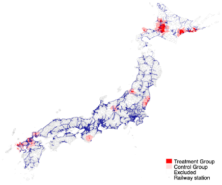
(a) 1931

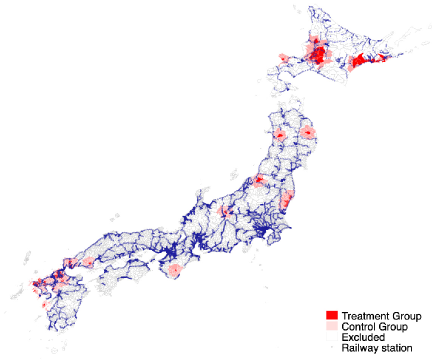
(b) 1936

Figure B.5: Spatial Distribution of Railway Stations

Notes: The blue circles indicate the location of railway stations. The base map used in this figure is Figure 2. The treatment (control) group highlighted in red (pink) includes the municipalities within 5 (between 5 and 30) km from a mine. The excluded municipalities are shown as empty lattices in the figures.

Source: Created by the author.

B.5 Seaports

Seaport locations were obtained from the official shapefile file created by the Ministry of Land, Infrastructure, Transport and Tourism (https://nlftp.mlit.go.jp/ksj/gmlold/datalist/gmlold˙KsjTmplt-C02.html, accessed 1st October 2022). The seaports used to match the 1931 (1936) mining dataset included all seaports (both commercial and fishery) listed in the 1931 (1936) edition of the Harbor Statistics of the Great Empire of Japan (Dainihon teikoku kōwan tōkei). The ports listed in the Harbor Statistics, but not included in the original shapefile of the Ministry of Land, Infrastructure, Transport, and Tourism, were added manually. Figure B.6a (B.6b) shows the distribution of seaports in 1931 (1936).

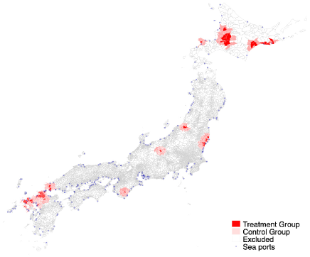
(a) 1931

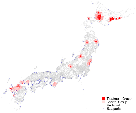
(b) 1936

Figure B.6: Spatial Distribution of Sea Ports

Notes: The blue circles indicate the location of seaports. The ports in Okinawa prefecture and a few ports in the islands far from the main island are not shown in the figures. The base map used in this figure is Figure 2. The treatment (control) group highlighted in red (pink) includes the municipalities within 5 (between 5 and 30) km from a mine. The excluded municipalities are shown as empty lattices in the figures.

Source: Created by the author.

B.6 Rivers

The location of rivers was obtained from the official shapefile provided by the Ministry of Land, Infrastructure, Transport, and Tourism (https://nlftp.mlit.go.jp/ksj/jpgis/datalist/KsjTmplt-W05.html, accessed August 21, 2018). The rivers used to match the mining dataset included those managed by the government or prefectures. As the rivers had not moved, the location information is time constant. Figure B.7a (B.7b) shows the distribution of the rivers matched to the 1931 (1936) base map.

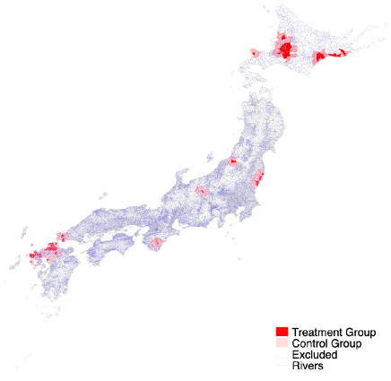
(a) 1931

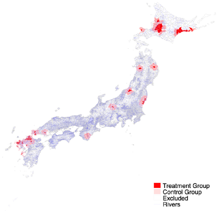
(b) 1936

Figure B.7: Spatial Distribution of Rivers

Notes: The blue lines indicate the location of rivers. The rivers in Okinawa prefecture and a few points in the islands far from the main island are not shown in the figures. The base map used in this figure is Figure 2. The treatment (control) group highlighted in red (pink) includes the municipalities within 5 (between 5 and 30) km from a mine. The excluded municipalities are shown as empty lattices in the figures.

Source: Created by the author.

B.7 Altitude

The grid cell data on altitude are taken from the official GIS database of the Ministry of Land, Infrastructure, Transport, and Tourism (https://nlftp.mlit.go.jp/ksj/gml/datalist/KsjTmplt-G04-d.html, accessed February 24, 2023). The average altitude in a 1 km square grid cell is calculated using the altitude measured in the 250 square grid cells in a third mesh-code initially assigned by the Ministry of Land, Infrastructure, Transport, and Tourism. The nearest neighbor grid cell is then linked to each municipality. The average distance to the nearest neighbor is $0.49$km, which is close enough to represent each municipality’s average altitude. Figure B.8 shows the spatial distribution of the altitude.

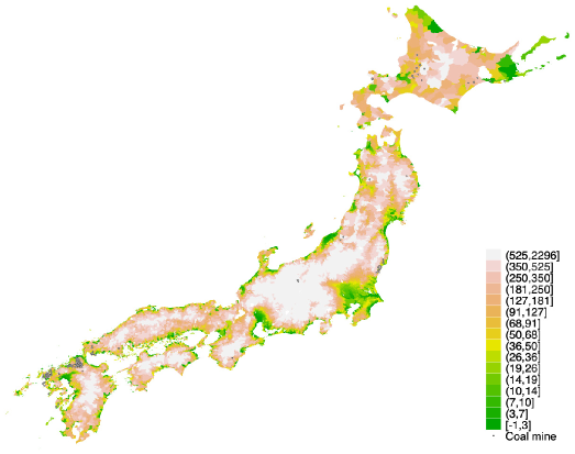
Figure B.8: Spatial Distribution of Altitude

Note: This figure illustrates the distribution of average altitude in each municipality. The rivers in Okinawa prefecture and a few points in the islands far from the main island are not shown in the figures. The white circles indicate the location of coal mines in 1936. Source: Created by the author.

Table B.5: Summary Statistics: Control Variables

	Year		Coal mines				GSC mines
Control Variables			Mean	Std. Dev.	Obs.		Mean	Std. Dev.	Obs.
Distance to station	1931		$5.38$	$5.84$	$1140$		$6.12$	$7.76$	$2498$
	1936		$5.62$	$6.18$	$1364$		$5.56$	$6.92$	$3293$
Distance to port	1931		$26.22$	$22.19$	$1140$		$29.87$	$22.22$	$2498$
	1936		$24.13$	$21.52$	$1364$		$32.66$	$24.28$	$3293$
Distance to river	1931		$0.99$	$1.59$	$1140$		$0.84$	$1.02$	$2498$
	1936		$1.02$	$1.55$	$1364$		$0.90$	$1.93$	$3293$

Notes: This table shows the summary statistics for the indicator variable for the treatment group and geological stratum. The geological stratum is a time constant variable: “Year” in parenthesis indicates the matched year. GSC mines indicate gold, silver, and copper mines. Distance to the nearest neighboring station/port/river is in kilometers.

Sources: Data on the location of mines are from the Association for Harmonious Cooperation (1932, 1937).

Appendix Appendix C Empirical Analysis Appendix

C.1 Attenuation due to Measurement Error

Consider a simplified projection of $y_{i}$ on $\textit{MineDeposit}_{i}$ as $y_{i}=\theta\textit{MineDeposit}_{i}+u_{i}$. When $\textit{MineDeposit}_{i}$ has a classical measurement error, as $\textit{MineDeposit}^{*}_{i}=\textit{MineDeposit}_{i}+u_{i}$, the observable model becomes $y_{i}=\theta^{*}\textit{MineDeposit}^{*}_{i}+\nu_{i}$. Consequently, I use $\text{cov}(\textit{MineDeposit}^{*}_{i},\nu_{i})=E[\textit{MineDeposit}^{*}_{i}\nu]=-\theta\text{var}(u_{i})\neq 0$ for $\theta^{*}=\theta+\text{cov}(\textit{MineDeposit}^{*}_{i},\nu_{i})/\text{var}(\textit{MineDeposit}^{*}_{i})$.

C.2 Assumptions for the Identification

To simplify the discussion on the identification assumptions, I focus on the most straightforward structural equation considered in this study, a dummy endogenous variable model taking the form:

$$\footnotesize{\begin{split}y_{i}=\alpha+\beta\text{{MineDeposit}}_{i}+e_{i},\\ \text{{MineDeposit}}_{i}=\kappa+\tau\text{{Stratum}}_{i}+\epsilon_{i}.\end{split}}$$ (6)

All the variables are those defined in Section 4. Note that I use the same Greek symbols to those used in equations 1 and 2 to simplify the expressions of the model, albeit those shall be different parameters to those considered in Section 4.

There are five assumptions to identify the parameter of interest under this setting: stable unit treatment value assumption (hereafter SUTVA), random assignments, exclusion restriction, nonzero average causal effect of the IV, and monotonicity (Angrist et al. 1996). Section 4 shows that the assumptions of the random assignments and exclusion restriction are essentially plausible given the nature of the spatial distributions of mines and stratums. In this subsection, I then discuss the rest of the three assumptions.

First, the SUTVA argues that the potential outcomes for municipality $i$ in the system (6) are only related to its own treatment status. Under my empirical setting that utilizes the municipal-level dataset, this assumption is less likely to be violated because there are certain distances among different treated municipalities, even in the agglomerated area such as Chikuhō coalfield. Moreover, to minimize the risk of SUTVA violation, I consider a certain threshold to define the treatment group. The results from the specifications show that the baseline definition of the treatment distance is plausible to model the potential spillover effects in the regression (Section C.4).

Second, let $\textit{MineDeposit}_{i}(\textit{Stratum}_{i})$ be an indicator for whether $i$ is treated given the random assignments of the geological strata, under the SUTVA. The nonzero average causal effect indicates that $E[\textit{MineDeposit}_{i}(1)-\textit{MineDeposit}_{i}(0)]\neq 0$. This assumption clearly holds because the likelihood of having coal mines increases with the IV strata (Online Appendix B.2).

Third, the monotonicity assumption suggests that $\forall i$, $\textit{MineDeposit}_{i}(1)\geq\textit{MineDeposit}_{i}(0)$. In sum, a combination of the nonzero average causal effect and monotonicity assumptions argue that strong monotonicity should be satisfied at least in one unit as $\textit{MineDeposit}_{i}(1)>\textit{MineDeposit}_{i}(0)$ (Angrist et al. 1996). Although this assumption is an idea for the potential outcome and is untestable (Imbens and Angrist 1994), there is fundamentally no reason for mining companies to avoid the stratum that contains coal seams. Thus, the instrument should affect the selection decision monotonically.

C.3 Alternative Variance Estimation

To assess the potential influences of the local-scale spatial correlations, I use the standard errors clustered at the county level based on the cluster-robust covariance matrix estimator (Arellano 1987). The finite-sample adjustment proposed by Hansen (2007) is implemented in the estimator. Table C.1 summarizes the results for the demographic outcomes, labor outcomes, and early-life health outcomes under the cluster-robust variance-covariance matrix estimator. All the results are materially similar to those of my baseline results in the main text.

Table C.1: Additional Results using the CRVE

Panel A-1: Population Growth (1930)
	(1) ln(Population)	(2) Sex Ratio	(3) HH Size	(4) Marrige	(5) Fertility	(6) Female MR
MineDeposit	$0.812***$	$0.115**$	$-0.438**$	$-2.584**$	$-7.020***$	$-1.851$
	$(0.234)$	$(0.045)$	$(0.190)$	$(1.019)$	$(2.092)$	$(1.642)$
Control variables	Yes	Yes	Yes	Yes	Yes	Yes
Observations	1,140	1,140	1,140	1,140	1,140	1,140
Panel A-2: Population Growth (1935)
MineDeposit	$0.895***$	$0.050*$	$-0.284$	$-1.386*$	$-1.144$	$-2.856**$
	$(0.193)$	$(0.028)$	$(0.216)$	$(0.741)$	$(2.212)$	$(1.395)$
Control variables	Yes	Yes	Yes	Yes	Yes	Yes
Observations	1,364	1,364	1,364	1,364	1,364	1,364
Panel B-1: Male Labor Supplies (1930)
	(1) LFP	(2) Mining	(3) Agricultural	(4) Manufacturing	(5) Commerce	(6) Domestic
MineDeposit	$-0.696$	$34.451***$	$-35.136***$	$1.752$	$-1.914$	$-0.439***$
	$(1.512)$	$(4.225)$	$(7.156)$	$(3.359)$	$(2.011)$	$(0.151)$
Control variables	Yes	Yes	Yes	Yes	Yes	Yes
Observations	1,140	1,140	1,140	1,140	1,140	1,140
Panel B-2: Female Labor Supplies (1930)
MineDeposit	$-18.930***$	$24.342***$	$-25.144***$	$-9.727***$	$3.057$	$4.731**$
	$(6.386)$	$(4.247)$	$(7.588)$	$(3.278)$	$(2.408)$	$(1.969)$
Control variables	Yes	Yes	Yes	Yes	Yes	Yes
Observations	1,140	1,140	1,140	1,140	1,140	1,140
Panel C-1: Early-life Health (1933)
	(1) IMR	(2) FDR	(3) FDR	(4) IMR	(5) CMR	(6) CMR
MineDeposit	$36.916$	$22.921**$			$-0.108$
	$(23.655)$	$(9.443)$			$(4.848)$
Female Miner			$0.034**$	$0.098***$		$0.004$
			$(0.013)$	$(0.034)$		$(0.004)$
Male Miner			$-0.002$	$-0.007*$		$-0.001$
			$(0.002)$	$(0.004)$		$(0.001)$
River accessibility	$-1.283$	$-0.393$	$-1.343$	$-0.552$	$-0.244$	$0.168$
	$(1.249)$	$(0.469)$	$(1.842)$	$(2.466)$	$(0.174)$	$(0.318)$
Control variables	Yes	Yes	Yes	Yes	Yes	Yes
Analytical sample	Full	Full	Treated	Treated	Full	Treated
Observations	1,140	1,140	93	93	1,140	93
Panel C-2: Early-life Health (1938)
MineDeposit	$17.412$	$6.680$			$1.717$
	$(16.220)$	$(11.385)$			$(3.306)$
Female Miner			$0.025*$	$0.066**$		$0.005$
			$(0.015)$	$(0.030)$		$(0.004)$
Male Miner			$0.001$	$0.000$		$0.000$
			$(0.001)$	$(0.002)$		$(0.000)$
River accessibility	$-1.162*$	$-0.379$	$0.279$	$-0.991$	$-0.286*$	$-0.278$
	$(0.623)$	$(0.435)$	$(1.601)$	$(1.640)$	$(0.168)$	$(0.393)$
Control variables	Yes	Yes	Yes	Yes	Yes	Yes
Analytical sample	Full	Full	Treated	Treated	Full	Treated
Observations	1,364	1,364	116	116	1,364	116

***, **, and * represent statistical significance at the 1%, 5%, and 10% levels, respectively. Standard errors based on the cluster-robust covariance matrix estimator are reported in parentheses. Standard errors are clustered at the 107 (124) counties in the 1933 (1938) sample.

Notes:

Panel A shows the results for the local population growth measured in the 1930 and 1935 Population Censuses. Panels A-1 and A-2 show the results for the 1930 and 1935 samples, respectively. Column (1) shows the result for the log-transformed population, whereas columns (2) and (3) show the results for mechanism analysis. Sex Ratio, HH Size, Marriage, Fertility, and Female MR indicate the sex ratio, average household size, crude marriage rate, crude birth rate, and female crude death rate, respectively (Panel B of Table B.4).

Panel B shows the results for the labor supplies measured in the 1930 Population Census. Panel B-1 and B-2 show the results for the male and female workers, respectively. Column (1) shows the main result for the labor force participation rate, whereas columns (2)–(5) show the results for the employment share in each industrial sector (Panel C of Table B.4).

Panel C shows the results for the early-life health measured in the 1933 and 1938 Vital Statistics. Panel C-1 and C-2 show the results for the 1933 and 1938 samples, respectively. IMR, FDR, and CMR indicate the infant mortality rate, fetal death rate, and child mortality rate, respectively (Panel B of Table B.4).

All the estimates listed are from the IV estimator. Control variables include the city and town fixed effects, railway accessibility, port accessibility, and river accessibility.

C.4 Testing the Validity of Threshold

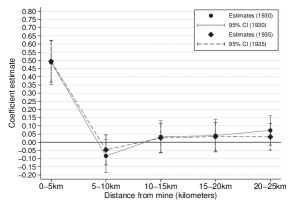
(a) Population

(b) IMR

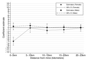
(c) LFP

Figure C.1: Heterogeneity in the Impact of Mines by Distance from the Mines

Notes: This figure shows the results from the expanded regressions of equation 1 that includes the five indicator variables for each 5km bin from a mine to 25 km away from the origin. 0–5 km distance from mines indicates the municipalities within 5 km of a mine. 5–10 (10–15, 15–20, 20–25) km distance from mines indicates the municipalities within $(5,10]$ ($(10,15],(15,20],(20,25]$) km of a mine. (20–30] km bin is used as a reference group.

Figures C.1a, C.1c, and C.1b show the results for the local population, labor force participation rate, and infant mortality rate (IMR), respectively. The dots and solid lines with caps show the estimates and their 95 percent confidence intervals, respectively. The confidence intervals are calculated using the standard errors based on the heteroskedasticity-robust covariance matrix estimator.

Source: Created by the author.

I test the validity of the threshold for the exposure variable (MineDeposit in 1) using my main outcome variables. In Figure C.1, I provide the results from the expanded regression of equation 1 that includes the five indicator variables for each 5 km bin from a mine. Figures C.1a, C.1b, and C.1c present the results for the population, IMR, and female labor force participation rate, respectively. Overall, the estimates are larger in the absolute sense within $5$ km, whereas those for the areas outside the 5 km bin are close to zero and statistically insignificant. This evidence provides a basis for defining the exposure variable that uses $5$ km as the threshold.

Only a 10-15 km bin for the infant mortality rate in 1938 shown in Figure C.1b shows a moderately positive estimate. The rest of this subsection assesses the potential mechanism behind the hike in the estimate for the 10–15 km bin in Figure C.1b.

First, to detect the region causing the hike, I split the entire sample into two subsamples: the municipalities belonging to Fukuoka prefecture and the others. The former might be an influential prefecture in the entire sample because it includes a number of mines in the Chikuhō coalfield. Figure C.2a shows the estimated coefficients for each subsample, suggesting that the hike originated from the Fukuoka prefecture variations.

Figure C.3a illustrates the distribution of the bins in Fukuoka. Figure C.3b clips the 10-15 km bin in the map. From a comparison of the distribution of the bins and the IMRs shown in Figure C.3c, it appears that some municipalities in the 10-15 km bin suffered a relatively higher risk of infant deaths, which is consistent with the tendency in Figure C.2a.

Notice that given a point of origin (i.e., a mine), a point on the concentric circle is a function of the distance. Therefore, to assess whether the hike in the 10-15 km bin is a random event or not, it is sufficient to check whether the location of mine is still endogenous and leading to the omitted variable bias, even after conditioning on the accessibility to railway stations, sea ports, and rivers.

A potential factor not considered in the baseline specification is the spatial distribution of the altitude. Terrain relates to the distribution of the locational fundamentals such as the climatic conditions (e.g., temperature and precipitation) and fixed cost of transportation. The climatic conditions are likely to affect agricultural productivity, suggesting that the altitude could be correlated with the opportunity cost of mining. Similarly, highlands are more expensive to transport, which may influence firm’s decisions on narrowly defined coal extraction areas.

To test this pathway, I created a new variable of the average altitude in each municipality using a set of grid cell datasets on the altitude (Online Appendix B.7). Figure C.3d shows the average altitude in each municipality in Fukuoka. Although this does not immediately provide a clear answer to the relationship between the location of mines and altitude, there is no specific correlation between both events. To delve into this relationship, I added the altitude as an additional control variable into the regressions in Figure C.2a. The result is shown in Figure C.2b, which is a nearly identical picture to Figure C.2a. Thus, the altitude is nearly independent to the location of mines.

To summarize, the hike observed in the 10-15 km bin shall be randomly occurred, but not be led by any systematic factors that relate to the distribution of mines. Given my empirical setting, this rather makes sense because using many bins reduces the available observations in each bin, making the moment estimator vulnerable to this kind of random shock.

Another evidence supporting this randomness is that such a hike in the 10-15km bin is not observed in the results for the 1933 sample (see Figure C.1b). If there were systematic factors, both 1933 and 1938 samples likely suffered the more significant risks of infant deaths in this bin. Similarly, the fact that only a 10-15 bin in Fukuoka prefecture suffers such a hike supports this argument. Overall, the hike is negligible in the sense that any systematic endogenous mechanism in the regression does not generate it.

(a) Baseline

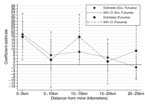
(b) Altitude Conditioned

Figure C.2: Heterogeneity in the Impact of Mines by Distance from the Mines:
The IMRs in 1938 in Fukuoka and Other Prefectures

Notes: This figure shows the results from the expanded regressions of Eq 1 that include the five indicator variables for each 5km bin from a mine to 25 km away from the origin. 0–5 km distance from mines indicates the municipalities within 5 km of a mine. 5–10 (10–15, 15–20, 20–25) km distance from mines indicates the municipalities within $(5,10]$ ($(10,15],(15,20],(20,25]$) km of a mine. (20–30] km bin is used as a reference group.

Figures C.1a, C.1c, and C.1b show the results for the local population, labor force participation rate, and infant mortality rate (IMR), respectively. The dots and solid lines with caps show the estimates and their 95 percent confidence intervals, respectively. The confidence intervals are calculated using the standard errors based on the heteroskedasticity-robust covariance matrix estimator.

Source: Created by the author.

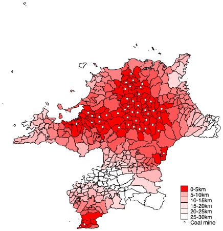
(a) Classification

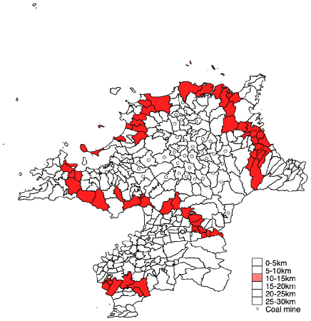
(b) 10-15 km Bins

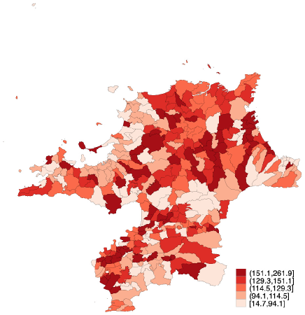
(c) IMR in 1938

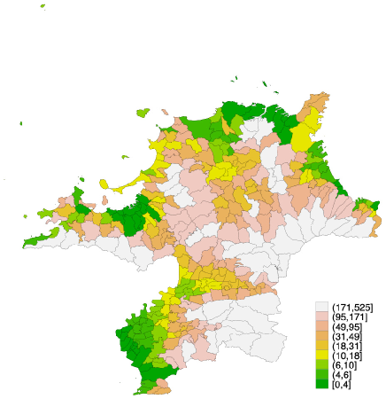
(d) Average Altitude

Figure C.3: Spatial Distribution of Rivers

Notes: Figure C.3a shows the spatial distribution of all the treatment bins used in Figure C.2. Figure C.3b highlights the location of the 10-15 km bin in Figure C.3a. Figures C.3c and C.3d show the infant mortality rates in 1938 and the average altitude in each municipality, respectively.

Source: Created by the author.

C.5 Sensitivity to the Altitude

The location of the mine might have been correlated with the altitude because terrain relates to the distribution of the locational fundamentals such as the climatic conditions and fixed cost of transportation. I confirmed that the results from the expanded regression including the average altitude in each municipality as an additional control variable show very similar results to my main results (not reported). Descriptions of the grid cell data on the average altitude are summarized in Online Appendix B.7.

C.6 Sensitivity to the Regional Heterogeneity in Endowment of Male Miners

I assess the influence of regional heterogeneity in female labor patterns. Nishinarita (1985) argues that, due to its geographical characteristics, coal mines in Hokkaidō (a northernmost island) tended to employ men from rural villages in the Tōhoku (northeastern) region of the main island as their main miners. This forced the coal mines in Hokkaidō to use a sloping-face haulage method instead of using ato-yama. As a result, female miners in the Hokkaido mines were mainly engaged in the coal selection process rather than working in pits. It is unlikely that this regional heterogeneity could affect the location of mines, because the location of coal mines depends on the presence or absence of coal-bearing strata (Section 4). In addition, the number of mines in Hokkaidō is relatively small, meaning that such regional heterogeneity in labor supply is less likely to disturb the estimates. Despite this, to test whether such features lead to omitted variable bias, I added an indicator variable for the municipalities of the Hokkaidō prefecture in the regressions. These results are similar to those of the main results listed in Tables 2,  5, and  4.

Table C.2 shows the results from the IV regressions, including an indicator variable for the municipalities in the Hokkaidō prefecture. Panels A, B, and C show the results for the population growth, labor supplies, and early-life health outcomes, respectively. The estimates listed in Panels A, B, and C are materially similar to those of my main results summarized in Tables 2, 5, and 4, respectively.

Table C.2: Additional Results: IV Regressions including a Hokkaidō Dummy

Panel A-1: Population Growth (1930)
	(1) ln(Population)	(2) Sex Ratio	(3) HH Size	(4) Marrige	(5) Fertility	(6) Female MR
MineDeposit	$0.922***$	$0.125**$	$-0.346**$	$-2.736**$	$-5.663***$	$-2.141$
	$(0.211)$	$(0.035)$	$(0.139)$	$(0.819)$	$(1.887)$	$(1.439)$
Control variables	Yes	Yes	Yes	Yes	Yes	Yes
Observations	1,140	1,140	1,140	1,140	1,140	1,140
Panel A-2: Population Growth (1935)
MineDeposit	$0.978***$	$0.059**$	$-0.207*$	$-1.512**$	$-0.426$	$-3.073***$
	$(0.194)$	$(0.023)$	$(0.123)$	$(0.664)$	$(1.560)$	$(1.132)$
Control variables	Yes	Yes	Yes	Yes	Yes	Yes
Observations	1,364	1,364	1,364	1,364	1,364	1,364
Panel B-1: Male Labor Supplies (1930)
	(1) LFP	(2) Mining	(3) Agricultural	(4) Manufacturing	(5) Commerce	(6) Domestic
MineDeposit	$-0.694$	$34.452***$	$-34.140***$	$1.752$	$-1.914$	$-0.439***$
	$(1.167)$	$(5.076)$	$(6.540)$	$(2.192)$	$(1.577)$	$(0.139)$
Control variables	Yes	Yes	Yes	Yes	Yes	Yes
Observations	1,140	1,140	1,140	1,140	1,140	1,140
Panel B-2: Female Labor Supplies (1930)
MineDeposit	$-18.931***$	$24.342***$	$-25.148***$	$-9.726***$	$3.058$	$4.731***$
	$(4.214)$	$(4.162)$	$(5.964)$	$(2.210)$	$(2.666)$	$(1.434)$
Control variables	Yes	Yes	Yes	Yes	Yes	Yes
Observations	1,140	1,140	1,140	1,140	1,140	1,140
Panel C-1: Early-life Health (1933)
	(1) IMR	(2) FDR	(3) FDR	(4) IMR	(5) CMR	(6) CMR
MineDeposit	$40.946**$	$21.558**$			$1.631$
	$(16.574)$	$(9.895)$			$(2.855)$
Female Miner			$0.029**$	$0.093***$		$0.006$
			$(0.012)$	$(0.033)$		$(0.004)$
Male Miner			$-0.002$	$-0.007*$		$-0.001$
			$(0.002)$	$(0.004)$		$(0.001)$
River accessibility	$-1.861**$	$-0.206$	$-0.090$	$-0.420$	$-0.492***$	$-0.137$
	$(0.893)$	$(0.543)$	$(1.498)$	$(2.611)$	$(0.149)$	$(0.290)$
Control variables	Yes	Yes	Yes	Yes	Yes	Yes
Analytical sample	Full	Full	Treated	Treated	Full	Treated
Observations	1,140	1,140	93	93	1,140	93
Panel C-2: Early-life Health (1938)
MineDeposit	$18.038$	$6.341$			$1.746$
	$(12.132)$	$(8.078)$			$(2.498)$
Female Miner			$0.025$	$0.065**$		$0.005$
			$(0.015)$	$(0.030)$		$(0.004)$
Male Miner			$0.001$	$0.000$		$0.000$
			$(0.001)$	$(0.002)$		$(0.000)$
River accessibility	$-1.274*$	$-0.324$	$0.439$	$-0.777$	$-0.342**$	$-0.294$
	$(0.669)$	$(0.491)$	$(1.645)$	$(1.667)$	$(0.159)$	$(0.433)$
Control variables	Yes	Yes	Yes	Yes	Yes	Yes
Analytical sample	Full	Full	Treated	Treated	Full	Treated
Observations	1,364	1,364	116	116	1,364	116

***, **, and * represent statistical significance at the 1%, 5%, and 10% levels, respectively. Standard errors based on the heteroskedasticity-robust covariance matrix estimator are reported in parentheses.

Notes:

Panel A shows the results for the local population growth measured in the 1930 and 1935 Population Censuses. Panels A-1 and A-2 show the results for the 1930 and 1935 samples, respectively. Column 1 shows the result for log-transformed population, whereas columns 2 and 3 show the results for mechanism analysis. Sex Ratio, HH Size, Marriage, Fertility, and Female MR indicate the sex ratio, average household size, crude marriage rate, crude birth rate, and female crude death rate, respectively (Panel B of Table B.4).

Panel B shows the results for the labor supplies measured in the 1930 Population Census. Panel B-1 and B-2 show the results for the male and female workers, respectively. Column 1 shows the main result for the labor force participation rate, whereas columns 2–5 show the results for the employment share in each industrial sector (Panel C of Table B.4).

Panel C shows the results for the early-life health measured in the 1933 and 1938 Vital Statistics. Panel C-1 and C-2 show the results for the 1933 and 1938 samples, respectively. IMR, FDR, and CMR indicate the infant mortality rate, fetal death rate, and child mortality rate, respectively (Panel B of Table B.4).

All the estimates listed are from the IV estimator. First-stage $F$-statistic values for each regression is similar to those reported in Tables 2, 5, and 4. Control variables include the city and town fixed effects, railway accessibility, port accessibility, river accessibility, and Hokkaidō dummy.

C.7 Alternative Identification Strategy

I used IV estimation to obtain the baseline estimates. For the outcome variables that can be used as a panel dataset, an alternative estimation strategy may be the DID approach, which uses both cross-sectional and within variations for the identification. To implement the DID technique, municipalities that had been treated throughout the measured years would have to be excluded, while municipalities that had newer mines during the sampled periods were left. However, the number of municipalities with coal mines increased by only 23 between 1931 and 1936 (Online Appendix A.3 presents the raw number of mines). Consequently, as explained in Section 3.1 in detail, the proportion of treated municipalities decreased from $15$% to $13$% (Panel A of Table B.3). This feature of the assignments makes it difficult to employ the DID approach as the main identification strategy for the coal mine sample because the information that can be used for the identification is insufficient.

Nevertheless, I provide a brief case study using the DID approach for the subsample, including Ogawa coal mine in Iwate prefecture and the Miyoshiyama coal mine in Akita prefecture. As indicated in Figure 2b, both mines were located in the northeastern (Tōhoku) region, where the coal mines did not exist in 1931. In this light, it is expected to provide relatively clean experimental conditions for the DID estimation, albeit the available sample size is limited.

For municipal $i$ at time $t\in\{1930,1935\}$, the two-way fixed effect (TWFE) model for the DID estimation is specified as follows:

$$\footnotesize{\begin{split}\textit{y}_{i,t}=\pi+\delta\textit{D}_{i,t}+\mathbf{x}^{\prime}_{i,t}\bm{\phi}+\eta_{i}+\lambda_{t}+\omega_{i,t},\end{split}}$$ (7)

where $\eta$, $\lambda$, and $\omega$ are the municipal fixed effect, year fixed effects, and random error term, respectively. $\textit{D}_{i,t}$ is a treatment indicator variable that takes one for the treatment group in the post-treatment period and zero for otherwise. $\mathbf{x}$ includes the accessibility measures on the stations and sea ports. Accessibility measure on the rivers is not included as it is a time-constant variable. However, the municipal fixed effect effectively controls for all these time-constant unobservable factors, including the geological strata and terrain that were potentially correlated with the location of mines.

Notice that this is a two-by-two DID setting for the TWFE model, which provides the unbiased DID estimator ($\hat{\delta}$) for the average treatment effect in the treated municipalities in the post-treatment period Abadie (2005). The identification assumptions are the independence of the treatment, which is confirmed already, and the parallel trends assumption. Figure C.4 shows the time-series plots of the outcome variables used in the DID analysis for the Iwate and Akita subsample in Table C.3. Although there are moderate fluctuations due to the small sample size in each group, these outcomes do not show peculiar trends but show the materially similar trends in the pretreatment years (i.e., 1925 and 1930). Notably, the outcomes of the treatment group in the post treatment period (i.e., 1935) show the clear kinks, whereas those for the control group show marginal changes in the post treatment period. A similar check for the IMR is unavailable because the data on the infant deaths in 1925 are unavailable.

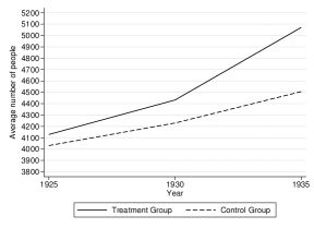
(a) Population

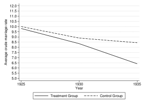
(b) Marriage

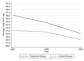
(c) Fertility

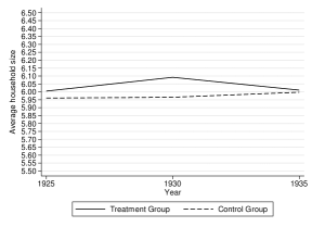
(d) Household Size

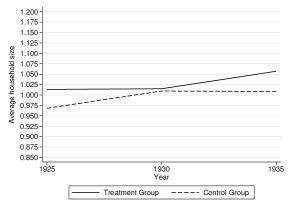
(e) Sex Ratio

Figure C.4: Trends in the Two Mining Areas in Iwate and Akita

Notes: This figure shows the time-series plots of the outcomes of the treatment and control groups in Iwate and Akita prefectures used in the regressions shown in Table C.3. Figures C.4a, C.4b, C.4c, C.4d, and C.4e show the average number of people, average crude marriage rate, average crude birth rate, average household size, and sex ratio, respectively. The data on the IMR in 1925 are unavailable.

Source: Created by the author.

The cluster-robust variance-covariance matrix estimator is used to deal with the heterosckedasticity and serial dependency (Arellano 1987).

Table C.3: Additional Results: Difference-in-Differences
for Two Coal Mine Areas in Iwate and Akita Prefectures

	Dependent Variable
	(1) Ln(Population)	(2) Marriage	(3) Fertility	(4) Size	(5) Sex Ratio	(6) IMR
MineDeposit	$0.072***$	$-1.478$	$-0.977$	$-0.101**$	$0.043***$	$22.350$
	$(0.025)$	$(1.506)$	$(2.558)$	$(0.050)$	$(0.011)$	$(24.066)$
Municipal and Year FEs	Yes	Yes	Yes	Yes	Yes	Yes
Railway accessibility	Yes	Yes	Yes	Yes	Yes	Yes
Port accessibility	Yes	Yes	Yes	Yes	Yes	Yes
Observations	136	136	136	136	136	136
Clusters	68	68	68	68	68	68
Years	1930 and 35	1930 and 35	1930 and 35	1930 and 35	1930 and 35	1933 and 38
Estimator	DID	DID	DID	DID	DID	DID

***, **, and * represent statistical significance at the 1%, 5%, and 10% levels, respectively. Standard errors based on the cluster-robust covariance matrix estimator are reported in parentheses.

Notes: This table shows the results for the coal mines subsample in Iwate and Akita prefectures. Column (1) shows the result for the log-transformed population. Columns (2)–(5) show the results for the crude marriage rate, crude birth rate, average household size, and sex ratio, respectively. Column (6) shows the result for the infant mortality rates. The results for the labor force participation rates are unavailable as those rates are measured only in the 1930 Population Census.

Table C.3 provides the results. Column (1) shows the result for the local population, whereas columns (2)–(5) show those for the crude marriage rate, crude birth rate, average household size, and sex ratio, respectively. Column (6) presents the result for the IMR. The results for the LFP rates are unavailable because those rates were measured only in one population census of 1930.

Overall, the DID results align with the findings from my baseline results. First, the opening of these two coal mines increased the local population by approximately $7.2$%. Although the estimated magnitude is much smaller than the baseline magnitude listed in Panel B-1 of Table 2, this is rather consistent with the fact that both coal mines are considerably smaller mines with roughly 100 miners. The results for the other demographic outcomes are also similar to those listed in Panel B-2 of Table 2. Second, the estimate for the IMR is positive but statistically insignificant, suggesting that the opening of coal mines did not increase the local infant mortality in the late 1930s. This is consistent with the fact that the impacts of coal mines on infant mortality could have been mitigated in the late 1930s by the regulations for the use of female miners in the pits (Section 6). In fact, both coal mines used few female miners: only 9 and 44 miners in Ogawa and Miyoshiyama coal mines, respectively.

C.8 Alternative Minerals: Heavy Metal Mines

Table C.4: Additional Results: Heavy Metal Mines

	Dependent Variable
	ln(Population)		LFP Rate in 1930		IMR
	(1) 1930	(2) 1935	(3) Male	(4) Female	(5) 1933	(6) 1938
MineDeposit	$0.160***$	$0.227***$	$-1.104***$	$-3.182***$	$-7.142**$	$-6.389**$
	$(0.047)$	$(0.049)$	$(0.321)$	$(0.942)$	$(3.107)$	$(3.013)$
City and Town FEs	Yes	Yes	Yes	Yes	Yes	Yes
Railway accessibility	Yes	Yes	Yes	Yes	Yes	Yes
Port accessibility	Yes	Yes	Yes	Yes	Yes	Yes
River accessibility	Yes	Yes	Yes	Yes	Yes	Yes
Observations	2,498	3,293	2,498	2,498	2,498	3,293
Estimator	OLS	OLS	OLS	OLS	OLS	OLS

***, **, and * represent statistical significance at the 1%, 5%, and 10% levels, respectively. Standard errors based on the heteroskedasticity-robust covariance matrix estimator are reported in parentheses.

Notes: This table shows the results for the GSC mines sample. Columns (1) and (2) show the results for the log-transformed population measured in the 1930 and 1935 population censuses, respectively. Columns (3) and (4) show the results for the labor force participation rates of male and female workers, respectively. Columns (5) and (6) show the results for the infant mortality rates (IMR) measured using the 1933 and 1938 vital statistics, respectively.

I assess the validity of my main results on coal mines by comparing the results for heavy metal mines. Specifically, I focus on three heavy metals: gold, silver, and copper (GSC). This is because GSC mines comprise more than $80$% of all metal mines and generally extract these metals at one place. Although the AHC documented other types of metal mines, they were indeed much smaller subsets: the number of lead and zinc, pig iron and steel, and tin mines recorded were only one, five, and four in 1931, respectively.

Historical evidence indicates that coal mining requires many more workers than heavy metal mining because coal is a bulky mineral (Section 2). Table B.3 indicates that the scale of GSC mines was much smaller than that of coal mines. In addition, unlike coal mines, the GSC mines were scattered across the archipelago and were less likely to agglomerate than coal mines (Online Appendix Figure B.2). In fact, the “enclave effect” suggests that some GSC mines are less likely to interact with local economies (Aragón and Rud 2013, 2015). This means that the impact of GSC mines on the regional economy would be smaller than those of coal mines. To assess this, I compare the estimates of the reduced-form equation 1 for the coal and GSC mines because unlike coal, a fuel mineral, no specific stratum can predict the spatial distribution of GSC mines.

Table C.4 lists the results. Panel A summarizes the results for the main outcome variables. The estimates for the local population listed in columns (1) and (2) are $0.160$ for 1930 sample and $0.227$ for 1935 sample, respectively. These are less than half of the estimates for the coal mine sample (column (3) of Panels A-1 and B-1 in Table 2). Similarly, columns (3) and (4) list smaller estimates for the labor force participation rates of male and female workers in mining areas (column (3) of Panels A-1 and B-1 in Table 5).

An interesting result was observed for the early life health outcomes. Generally, heavy metal mining releases toxic metals, such as mercury (Hg), cyanide (CN), and cadmium (Cd), which are associated with incidences of miscarriages and stillbirths (Amadi et al. 2017). However, columns (5) and (6) indicate that the results for IMRs are rather negative and statistically significant. This means that infant mortality risk is even lower in the GSC mining areas than that in the surrounding municipalities. Investigating this difference is beyond the scope of this study; however, this result suggests that unlike in coal mines, the positive economic effect of mines may exceed the adverse health effects, as found in a recent related study by Benshaul-Tolonen (2019). My results also support Drixler (2016), who found that industrial pollution from copper mines was not associated with the risk of high stillbirth rates in Japan in the late 19th century. In addition, this difference may be related to the characteristics of the pollutants. While particulates generated around coal mines may immediately deteriorate the mother’s and infant’s health conditions, the heavy metals from GSC mines might not immediately affect mothers. In other words, my empirical setting does not capture the accumulation effects of heavy metals on humans.

C.9 Time-Series Plots of the IMR and FDR

Figure C.5 shows the national average IMR (solid line) and FDRs (dashed line). Both series show secular decreasing trends between 1925 and 1940.

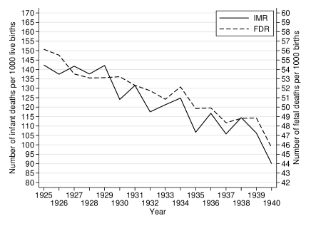
Figure C.5: The Infant Mortality and Fetal Death Rates
between 1925 and 1940

Note: This figure shows the national average infant mortality (IMR; solid line) and fetal death rates (FDR; dashed line) in Japan between 1925 and 1940. The IMR is the number of infant deaths per 1,000 live births. The FDR is defined as the number of fetal deaths per 1,000 births.

Sources: Created by the author. Data on the number of infant and fetal deaths are from the Statistics Bureau of the Cabinet (1926–1942).

C.10 Heterogeneity with Respect to Scale of Mines

While most of the municipalities with mines have a similar number of mines (i.e., one or two mines), there are several municipalities having many mines. Importantly, the causal effects are essentially heterogeneous across municipalities. This means that the municipalities with large-scale mine could have more significant impacts than those with small-scale mine. Estimating the heterogeneous treatment effects in detail is out of scope in this study. As explained, I am rather interested in estimating the LATE utilizing the IV approach. There also be a practical issue in estimating such varying effects: stratifying the treatment group disturbs the inference due to the small sample size in each subsample.

Despite this, it may be useful to see whether the potential heterogeneity in the treatment effect concerning scale of mines is reasonable. To assess the heterogeneity, I first stratify the treatment group into two subgroups using the median of the number of miners as a threshold. The key treatment indicator variable in equation 1 is then replaced with the two indicator variables for the two subgroups.

Table C.5 presents the results for the local population (columns (1) and (2)), labor force participation rates (columns (3) and (4)), and early-life health outcomes (columns (5) and (6)). Columns (1) and (2) suggest that the relatively large-scale mines had more significant impacts on the local population growth. Column (3) indicates that the impacts on the male labor force participation did not relate to the scale of mines, whereas column (4) suggests that the declines in the female labor force participation were mainly observed in the municipalities with relatively larger scale mines. Column (5) shows that the coal mines increased the risk of infant mortality regardless of the scale of mines in 1933, whereas column (6) indicates that the effects of relatively small-scale mines disappeared in 1938 and those of relatively large-scale mines also declined from 1933. This result is rather consistent with my baseline finding, which supports the effectiveness of the revised regulations.

Table C.5: Additional Results: Heterogeneity with Respect to the Scale of Mines

	Dependent Variable
	ln(Population)		LFP Rate in 1930		IMR
	(1) 1930	(2) 1935	(3) Male	(4) Female	(5) 1933	(6) 1938
MineDeposit ($\leq$ median)	$0.136**$	$0.176**$	$0.605$	$-0.966$	$18.108***$	$7.550$
	$(0.062)$	$(0.071)$	$(0.420)$	$(1.017)$	$(5.687)$	$(4.875)$
MineDeposit ($>$ median)	$0.674***$	$0.616***$	$-0.645$	$-7.881***$	$25.848***$	$21.698***$
	$(0.080)$	$(0.074)$	$(0.400)$	$(1.136)$	$(4.684)$	$(3.512)$
City and Town FEs	Yes	Yes	Yes	Yes	Yes	Yes
Railway accessibility	Yes	Yes	Yes	Yes	Yes	Yes
Port accessibility	Yes	Yes	Yes	Yes	Yes	Yes
River accessibility	Yes	Yes	Yes	Yes	Yes	Yes
Observations	1,140	1,364	1,140	1,140	1,140	1,364
Estimator	OLS	OLS	OLS	OLS	OLS	OLS

***, **, and * represent statistical significance at the 1%, 5%, and 10% levels, respectively. Standard errors based on the heteroskedasticity-robust covariance matrix estimator are reported in parentheses.

Notes: MineDeposit ($\leq$ median) indicates an indicator variable for the municipalities within 5km from a mine, which had the number of miners less than or equals to median. MineDeposit ($>$ median) indicates an indicator variable for the municipalities within 5km from a mine, which had the number of miners more than median. Columns (1) and (2) show the results for the log-transformed population measured in the 1930 and 1935 population censuses, respectively. Columns (3) and (4) show the results for the labor force participation rates of male and female workers, respectively. Columns (5) and (6) show the results for the infant mortality rates measured using the 1933 and 1938 vital statistics, respectively.

C.11 Conditional Expectation of the Truncated Normal Distribution

Let $x\sim\mathcal{N}(\mu,\,\sigma^{2})$ be the initial health endowment of a fetus in utero and $x_{s}$ be a survival threshold. The conditional expectation of the truncated normal distribution can be derived as:

$$\footnotesize{\begin{split}E[x|x>x_{s}]&=\int_{x_{s}}^{\infty}x\frac{f(x)}{1-F(x_{s})}dx\\ &=\frac{-\sigma^{2}}{1-F(x_{s})}\int_{x_{s}}^{\infty}-\frac{(x-\mu)}{\sigma^{2}}f(x)dx+\frac{\mu}{1-F(x_{s})}\int_{x_{s}}^{\infty}f(x)dx\\ &=\mu+\sigma^{2}\frac{f(x_{s})}{1-F(x_{s})}.\end{split}}$$

This implies that while the “scarring” mechanism ($\mu^{*}<\mu$) shifts the conditional mean toward the left, the “selection” mechanism ($x_{s}^{*}>x_{s}$) shifts the conditional mean toward the right.

References

- Abramitzky et al. (2011) Ran Abramitzky, Adeline Delavande, and Luis Vasconcelos. Marrying Up: The Role of Sex Ratio in Assortative Matching. American Economic Journal: Applied Economics, 3(3):124–157, July 2011.
- Acemoglu and Shimer (1999) Daron Acemoglu and Robert Shimer. Efficient unemployment insurance. The Journal of Political Economy, 107(5):893–928, 1999.
- Acemoglu et al. (2001) Daron Acemoglu, Simon Johnson, and James A Robinson. The colonial origins of comparative development: An empirical investigation. American Economic Review, 91(5):1369–1401, December 2001.
- Ahmed and Jaakkola (2007) Parvez Ahmed and Jouni J K Jaakkola. Maternal occupation and adverse pregnancy outcomes: a finnish population-based study. Occupational Medicine, 57(6):417–423, September 2007.
- Allcott and Keniston (2018) Hunt Allcott and Daniel Keniston. Dutch disease or agglomeration? the local economic effects of natural resource booms in modern america. The Review of Economic Studies, 85(2 (303)):695–731, 2018.
- Amadi et al. (2017) Cecilia Nwadiuto Amadi, Zelinjo Nkeiruka Igweze, and Orish Ebere Orisakwe. Heavy metals in miscarriages and stillbirths in developing nations. Middle East Fertility Society Journal, 22(2):91–100, June 2017.
- Angrist (2002) Josh Angrist. How do sex ratios affect marriage and labor markets? Evidence from America’s second generation. Quarterly Journal of Economics, 117(3):997–1038, August 2002.
- Aragón and Rud (2013) Fernando M Aragón and Juan Pablo Rud. Natural Resources and Local Communities: Evidence from a Peruvian Gold Mine. American Economic Journal: Economic Policy, 5(2):1–25, May 2013.
- Aragón and Rud (2015) Fernando M Aragón and Juan Pablo Rud. Polluting industries and agricultural productivity: Evidence from mining in Ghana. The Economic Journal, 126(597):1980–2011, September 2015.
- Arellano (1987) Manuel Arellano. Computing standard errors for robust within-groups estimators. Oxford Bulletin of Economics and Statistics, 49(4):431–434, November 1987.
- Association for Harmonious Cooperation (1932) Association for Harmonious Cooperation. Zenkoku kōjyōkōzan meibo (The lists of factories and mines, 1932 edition). [in Japanese]. Association for Harmonious Cooperation, Tokyo, 1932.
- Association for Harmonious Cooperation (1937) Association for Harmonious Cooperation. Zenkoku kōjyōkōzan meibo (The lists of factories and mines, 1937 edition). [in Japanese]. Association for Harmonious Cooperation, Tokyo, 1937.
- Beach and Hanlon (2017) Brian Beach and W Walker Hanlon. Coal Smoke and Mortality in an Early Industrial Economy. The Economic Journal, 128(615):2652–2675, November 2017.
- Benshaul-Tolonen (2019) Anja Benshaul-Tolonen. Local Industrial Shocks and Infant Mortality. The Economic Journal, 129(620):1561–1592, May 2019.
- Besley and Burgess (2004) Timothy Besley and Robin Burgess. Can labor regulation hinder economic performance? evidence from india. The Quarterly Journal of Economics, 119(1):91–134, 2004.
- Bjørnland and Thorsrud (2016) Hilde C Bjørnland and Leif A Thorsrud. Boom or Gloom? Examining the Dutch Disease in Two-speed Economies. The Economic Journal, 126(598):2219–2256, May 2016.
- Black et al. (2005) Dan Black, Terra McKinnish, and Seth Sanders. The economic impact of the coal boom and bust. The Economic Journal, 115(503):449–476, April 2005.
- Botero et al. (2004) Juan C Botero, Simeon Djankov, Rafael La Porta, Florencio Lopez-de Silanes, and Andrei Shleifer. The regulation of labor. The Quarterly Journal of Economics, 119(4):1339–1382, 2004.
- Caselli and Coleman II (2001) Francesco Caselli and Wilbur John Coleman II. The U.S. structural transformation and regional convergence: A reinterpretation. The Journal of Political Economy, 109(3):584–616, June 2001.
- Caselli and Guy (2009) Francesco Caselli and Michaels Guy. Do oil windfalls improve living standards? Evidence from Brazil. NBER Working Paper, 15550:1–60, December 2009.
- Caselli and Guy (2013) Francesco Caselli and Michaels Guy. Do Oil Windfalls Improve Living Standards? Evidence from Brazil. American Economic Journal: Applied Economics, 5(1):208–238, January 2013.
- Chiba and Yamada (1964) Hiroshi Chiba and Takashi Yamada. Chikuhō coalfield and onga river [in japanese]. Suiri kagaku, 8(1):88–103, 1964.
- Corden (1984) Max W Corden. Booming sector and Dutch disease economics: Survey and consolidation. Oxford Economic Papers, 36(3):359–380, November 1984.
- Corden and Neary (1982) Max W Corden and J Peter Neary. Booming sector and de-industrialisation in a small open economy. The Economic Journal, 92(368):825–848, December 1982.
- Djankov et al. (2002) Simeon Djankov, Rafael La Porta, Florencio Lopez-de Silanes, and Andrei Shleifer. The regulation of entry. The Quarterly Journal of Economics, 117(1):1–37, February 2002.
- Domenech (2008) Jordi Domenech. Mineral resource abundance and regional growth in Spain, 1860-2000. Journal of International Development, 20(8):1122–1135, November 2008.
- Drixler (2016) Fabian F Drixler. Hidden in Plain Sight: Stillbirths and Infanticides in Imperial Japan. The Journal of Economic History, 76(3):651–696, September 2016.
- Duranton and Puga (2004) Gilles Duranton and Diego Puga. Micro-foundations of urban agglomeration economies. In Vernon J Henderson and Jacques-François Thisse, editors, Handbook of Regional and Urban Economics, vol.4, pages 2063–2117. Elsevier, Amsterdam, 2004.
- Eastwood and Venables (1982) R K Eastwood and A J Venables. The macroeconomic implications of a resource discovery in an open economy. The Economic Journal, 92(366):285–299, June 1982.
- Fernández-Villaverde (2018) Jesús Fernández-Villaverde. The economic consequences of labor market regulations. University of Chicago Legal Forum, 2017(6), 2018.
- Fernihough and O’Rourke (2020) Alan Fernihough and Hjortshøj Kevin O’Rourke. Coal and the European Industrial Revolution. The Economic Journal, 131(635):1135–1149, April 2020.
- Freeman (1993) Richard B Freeman. Labor markets and institutions in economic development. American Economic Review, 83(2):403–408, 1993.
- Grönqvist et al. (2017) Hans Grönqvist, Peter J Nilsson, and Pre-Olof Robling. Early lead exposure and outcomes in adulthood. IFAU Working Paper, 4:1–72, May 2017.
- Hall and Jones (1999) Robert E Hall and Charles I Jones. Why do some countries produce so much more output per worker than others? The Quarterly Journal of Economics, 114(1):83–116, 1999.
- Hanlon (2020) Walker W Hanlon. Coal smoke, city growth, and the costs of the industrial revolution. The Economic Journal, 130(626):462–488, February 2020.
- Heblich et al. (2018) Stephan Heblich, Alex Trew, and Yanos Zylberberg. East side story: Historical pollution and persistent neighborhood sorting. School of Economics and Finance Discussion Papers, pages 1–77, March 2018.
- Hinkley (1977) David V Hinkley. Jackknifing in unbalanced situations. Technometrics, 19(3):285–292, August 1977.
- Horn et al. (1975) Susan D Horn, Roger A Horn, and David B Duncan. Estimating Heteroscedastic Variances in Linear Models. Journal of the American Statistical Association, 70(350):380–385, June 1975.
- Ishii (1991) Kanji Ishii. Japanese Economic History, second edition [in Japanese]. University of Tokyo Press, Tokyo, 1991.
- Ito (1990) Shigeru Ito. Population growth, urbanization, and employment structure. In Shumsaku Nishikawa and Arizo Yamamoto, editors, Japanese Economic History, volume.5 [in Japanese], pages 227–239. Iwanami Shoten, Tokyo, 1990.
- Japan Mining Association (1928) Japan Mining Association. Nihon kōzan kyōkai siryō, dai isshū (Japan Mining Association Materials, volume 1). [in Japanese]. Japan Mining Association, Tokyo, 1928.
- Japan Mining Association (1930) Japan Mining Association. Nihon kōzan kyōkai siryō, dai jyūyon shū (Japan Mining Association Materials, volume 14). [in Japanese]. Japan Mining Association, Tokyo, 1930.
- Japan Mining Association (1931) Japan Mining Association. Nihon kōzan kyōkai siryō, dai jyūgo shū (Japan Mining Association Materials, volume 15). [in Japanese]. Japan Mining Association, Tokyo, 1931.
- Kotsadam and Tolonen (2016) Andreas Kotsadam and Anja Tolonen. African mining, gender, and local employment. World Development, 83:325–339, July 2016.
- Landrigan et al. (2017) Philip J Landrigan, Richard Fuller, Nereus J R Acosta, Olusoji Adeyi, Robert Arnold, Niladri Nil Basu, Abdoulaye Bibi Baldé, Roberto Bertollini, Stephan Bose-O’Reilly, Jo Ivey Boufford, Patrick N Breysse, Thomas Chiles, Chulabhorn Mahidol, Awa M Coll-Seck, Prof Maureen L Cropper, Julius Fobil, Valentin Fuster, Michael Greenstone, Andy Haines, David Hanrahan, David Hunter, Mukesh Khare, Alan Krupnick, Bruce Lanphear, Bindu Lohani, Keith Martin, Karen V Mathiasen, Maureen A McTeer, Christopher J L Murray, Johanita D Ndahimananjara, Frederica Perera, Janez PotoÄ nik, Alexander S Preker, Jairam Ramesh, Johan Rockström, Carlos Salinas, Leona D Samson, Karti Sandilya, Peter D Sly, Kirk R Smith, Achim Steiner, Richard B Stewart, William A Suk, van Schayck Onno C P, Gautam N Yadama, Kandeh Yumkella, and Ma Zhong. The Lancet Commission on pollution and health. The Lancet, 391(10119):1–51, October 2017.
- Lederman and Maloney (2007) Daniel Lederman and William F. Maloney. Natural resources: Neither curse nor destiny. Stanford University Press, Washington, 2007.
- Lin et al. (2013) Ja-Liang Lin, Pao-Hsien Chu, Dan-Tzu Lin-Tan, Ching-Wei Hsu, Wen-Hung Huang, Kuan-Hsing Chen, and Tzung-Hai Yen. Cadmium excretion predicting 30-day mortality and illness severity of patients with acute myocardial infarction. International Journal of Cardiology, 168(5):4822–4824, October 2013.
- Mathias (2001) Peter Mathias. The First Industrial Nation: An Economic History of Britain, 1700-1914, 3rd edition. Routledge, 2001.
- Michaels (2010) Guy Michaels. The long term consequences of resource-based specialisation. The Economic Journal, 121(551):31–57, November 2010.
- Minami (1994) Ryōshin Minami. The Economic Development of Japan: A Quantitative Study, Second Edition. The Macmillan Press, Hampshire, 1994.
- Mining Bureau, Ministry of Commerce and Industry (1934) Mining Bureau, Ministry of Commerce and Industry. Hongoku kogyō no sūsei (Trend of mining in Japan, 1933 edition). [in Japanese]. Mining Bureau, Ministry of Commerce and Industry, Tokyo, 1934.
- Ministry of Commerce and Industry (1926) Ministry of Commerce and Industry. Honpou jyūyō kōzan yōran (Handbook of Important Mines in Japan). [in Japanese]. Bureau of Mines, Ministry of Commerce and Industry, Tokyo, 1926.
- Ministry of International Trade and Industry (1954) Ministry of International Trade and Industry. Honpō kogyō no sūsei (Trends in Mining Industry of Japan, 1950 edition). [in Japanese]. Ministry of International Trade and Industry, Tokyo, 1954.
- Mokyr (1977) Joel Mokyr. Industrialization in the Low Countries, 1795-1850. Yale University Press, New Haven, CT, 1977.
- Morimoto (2013) Mayo Morimoto. Naibu rōdō shijyō no keisei (Formation of Internal Labor Market). In Masaki Nakabayashi, editor, Long Wave of Modernization in the Japanese Economy [in Japanese], pages 259–302. University of Tokyo Press, Tokyo, 2013.
- Nakamura (1971) Takafusa Nakamura. An analysis of the economic growth in prewar Japan. [in Japanese]. Iwanami shoten, Tokyo, 1971.
- Neary and van Wijnbergen (1984) J Peter Neary and S van Wijnbergen. Can an oil discovery lead to a recession? A comment on eastwood and venables. The Economic Journal, 94(374):390–395, January 1984.
- Nickell and Laynard (1999) Stephen Nickell and Richard Laynard. Labor market institutions and economic performance. In Orley C Ashenfelter and David Card, editors, Handbook of Labor Economics, Volume 3, Part C, pages 3029–3084. North-Holland, Amsterdam, 1999.
- Nishinarita (1985) Yutaka Nishinarita. Jyoshirōdō no shoruikei to sono henyō. In Masanori Nakamura, editor, Technological Innovation and Women’s Labor [in Japanese], pages 71–106. Tokyo Daigaku Shuppan Kai, Tokyo, 1985.
- Notehelfer (1975) Fred G Notehelfer. Japan’s first pollution incident. Journal of Japanese Studies, 1(2):351–383, 1975.
- Okazaki (2021) Tetsuji Okazaki. Intrafirm resource reallocation and labor productivity growth in the Japanese coal mining industry: Comparative study on Mitsubishi Mining Co., Mitsui Mining Co., and Hokkaido Colliery & Steamship Co. in the 1930s [in Japanese]. CIGS Working Paper Series, 21-001J:1–23, September 2021.
- Papyrakis and Gerlagh (2007) Elissaios Papyrakis and Reyer Gerlagh. Resource abundance and economic growth in the United States. European Economic Review, 51(4):1011–1039, May 2007.
- Pollard (1981) Sidney Pollard. Peaceful Conquest: The Industrialization of Europe, 1760-1970. Oxford University Press, 1981.
- Rosenthal and Strange (2004) Stuart S Rosenthal and William C Strange. Evidence on the nature and sources of agglomeration economies. In Vernon J Henderson and Jacques-François Thisse, editors, Handbook of Regional and Urban Economics, vol.4, pages 2119–2171. Elsevier, Amsterdam, 2004.
- Sachs and Warner (1999) Jeffrey D Sachs and Andrew M Warner. The big push, natural resource booms and growth. Journal of Development Economics, 59(1):43–76, June 1999.
- Sachs and Warner (2001) Jeffrey D Sachs and Andrew M Warner. The curse of natural resources. European Economic Review, 45(4-6):827–838, May 2001.
- Sergeant et al. (2022) Christopher J Sergeant, Erin K Sexton, Jonathan W Moore, Alana R Westwood, Sonia A Nagorski, Joseph L Ebersole, David M Chambers, Sarah L O’Neal, Rachel L Malison, F Richard Hauer, Diane C Whited, Jill Weitz, Jackie Caldwell, Marissa Capito, Mark Connor, Christopher A Frissell, Greg Knox, Erin D Lowery, Randal Macnair, Vicki Marlatt, Jenifer K McIntyre, Megan V McPhee, and Nikki Skuce. Risks of mining to salmonid-bearing watersheds. Science Advances, 8(26):eabn0929, July 2022.
- Staiger and Stock (1997) Douglas Staiger and James H. Stock. Instrumental variables regression with weak instruments. Econometrica, 65(3):557–586, May 1997.
- Statistics Bureau of the Cabinet (1926) Statistics Bureau of the Cabinet. Rodō tōkei jitchi chōsa hōkoku, Taisho jyūsan nen, Kōzan no bu (Labor statistics field survey report, 1924 edition, Mine section). [in Japanese]. Statistics Bureau of the Cabinet, Tokyo, 1926.
- Statistics Bureau of the Cabinet (1930) Statistics Bureau of the Cabinet. Rodō tōkei jitchi chōsa hōkoku, Shōwa ni nen dai yonkan, Kōzan no bu (Labor statistics field survey report, 1927 edition, volume 4, Mine section). [in Japanese]. Statistics Bureau of the Cabinet, Tokyo, 1930.
- Statistics Bureau of the Cabinet (1932a) Statistics Bureau of the Cabinet. Rodō tōkei jitchi chōsa hōkoku, Shōwa ni nen dai ikkan, Kijyutsu no bu (Labor statistics field survey report, 1927 edition, volume 1, description). [in Japanese]. Statistics Bureau of the Cabinet, Tokyo, 1932a.
- Statistics Bureau of the Cabinet (1932b) Statistics Bureau of the Cabinet. Rodō tōkei jitchi chōsa hōkoku, Shōwa go nen dai nikan, Kōzan no bu (Labor statistics field survey report, 1930 edition, volume 2, Mine section). [in Japanese]. Statistics Bureau of the Cabinet, Tokyo, 1932b.
- Statistics Bureau of the Cabinet (1932c) Statistics Bureau of the Cabinet. Shichōsonbetsu jinkōdōtaitōkei (The vital statistics for municipalities, 1930 edition). [in Japanese]. Statistics Bureau of the Cabinet, Tokyo, 1932c.
- Statistics Bureau of the Cabinet (1935a) Statistics Bureau of the Cabinet. Shōwagonen Kokuseichōsahōkoku, fukenhen (1930 Population Census of Japan, prefectural part). [in Japanese]. Statistics Bureau of the Cabinet, Tokyo, 1935a.
- Statistics Bureau of the Cabinet (1935b) Statistics Bureau of the Cabinet. Shōwagonen Kokuseichōsahōkoku, daiikkan (1930 Population Census of Japan, volume 1). [in Japanese]. Statistics Bureau of the Cabinet, Tokyo, 1935b.
- Statistics Bureau of the Cabinet (1936) Statistics Bureau of the Cabinet. Rodō tōkei jitchi chōsa hōkoku, Shōwa hachi nen dai nikan, Kōzan no bu (Labor statistics field survey report, 1933 edition, volume 2, Mine section). [in Japanese]. Statistics Bureau of the Cabinet, Tokyo, 1936.
- Statistics Bureau of the Cabinet (1937) Statistics Bureau of the Cabinet. Rodō tōkei jitchi chōsa hōkoku, Shōwa jyūichi nen dai nikan, dai ichi bu (Labor statistics field survey report, 1936 edition, volume 2, First section). [in Japanese]. Statistics Bureau of the Cabinet, Tokyo, 1937.
- Statistics Bureau of the Cabinet (1938) Statistics Bureau of the Cabinet. Shichōsonbetsu jinkōdōtaitōkei (The vital statistics for municipalities, 1935 edition). [in Japanese]. Statistics Bureau of the Cabinet, Tokyo, 1938.
- Statistics Bureau of the Cabinet (1939) Statistics Bureau of the Cabinet. Shōwajyūnen Kokuseichōsahōkoku, daiikkan (1935 Population Census of Japan, volume 1). [in Japanese]. Statistics Bureau of the Cabinet, Tokyo, 1939.
- Sumiya (1968) Mikio Sumiya. Nihon sekitan sangyō bunseki (Study of Japanese Coal Industry). [in Japanese]. Iwanami Shoten, Tokyo, 1968.
- Tanaka and Ogino (1977) Naoki Tanaka and Yoshihiro Ogino. Miners protection issue and rationalization of coal extraction mechanism [in Japanese]. Enerugī-shi kenkyū, 8:74–82, June 1977.
- Tobin (1958) James Tobin. Estimation of relationships for limited dependent variables. Econometrica, 26(1):24–36, January 1958.
- Trivers and Willard (1973) Robert L Trivers and Dan E Willard. Natural Selection of Parental Ability to Vary the Sex Ratio of Offspring. Science, 179(4068):90–92, January 1973.
- Valente (2015) Christine Valente. Civil conflict, gender-specific fetal loss, and selection: A new test of the Trivers–Willard hypothesis. Journal of Health Economics, 39:31–50, January 2015.
- van Wijnbergen (1984) Sweder van Wijnbergen. The ‘Dutch Disease’: A disease after all? The Economic Journal, 94(373):41–55, March 1984.
- von der Goltz and Barnwal (2019) Jan von der Goltz and Prabhat Barnwal. Mines: The local wealth and health effects of mineral mining in developing countries. Journal of Development Economics, 139:1–16, June 2019.
- Wilson (2012) Nicholas Wilson. Economic booms and risky sexual behavior: Evidence from Zambian copper mining cities. Journal of Health Economics, 31(6):797–812, December 2012.