Signal and Image Reconstruction with Tight Frames via Unconstrained $\ell_{1}-\alpha\ell_{2}$-Analysis Minimizations

Abstract

In the paper, we introduce an unconstrained analysis model based on the $\ell_{1}-\alpha\ell_{2}$ $(0<\alpha\leq 1)$ minimization for the signal and image reconstruction. We develop some new technology lemmas for tight frame, and the recovery guarantees based on the restricted isometry property adapted to frames. The effective algorithm is established for the proposed nonconvex analysis model. We illustrate the performance of the proposed model and algorithm for the signal and compressed sensing MRI reconstruction via extensive numerical experiments. And their performance is better than that of the existing methods.

Key Words and Phrases. Unconstrained $\ell_{1}-\alpha\ell_{2}$-analysis, Tight frame, Restricted isometry property, Restricted orthogonality constant.

MSC 2020. 94A12, 90C26, 42C15

1 Introduction

1.1 Sparse Signal Reconstruction

In compressed sensing (CS), a crucial concern is to reconstruct a high-dimensional signals from a relatively small number of linear measurements

$$\bm{b}=\bm{A}\bm{x}+\bm{e},$$ (1.1)

where $\bm{b}\in\mathbb{R}^{m}$ is a vector of measurements, $\bm{A}\in\mathbb{R}^{m\times n}~{}(m\ll n)$ is a sensing matrix modeling the linear measurement process, $\bm{x}\in\mathbb{R}^{n}$ is an unknown sparse or compressible signal and $\bm{e}\in\mathbb{R}^{m}$ is a vector of measurement errors, see, e.g., [8, 14]. To reconstruct $\bm{x}$, the most intuitive approach is to find the sparsest signal, that is, one solves via the $\ell_{0}$ minimization problem:

$$\min_{\bm{x}\in\mathbb{R}^{n}}\|\bm{x}\|_{0}~{}~{}\text{subject~{} to}~{}~{}\bm{b}-\bm{A}\bm{x}\in\mathcal{B},$$ (1.2)

where $\|\bm{x}\|_{0}$ is the number of nonzero coordinates of $\bm{x}$ and $\mathcal{B}$ is a bounded set determined by the error structure. It is known that the problem (1.2) is NP-hard for high dimensional signals and faces challenges in both theoretical and computational (see, e.g., [15, 42, 54]). Then many fast and effective algorithms have been developed to recover $\bm{x}$ from (1.1). The Least Absolute Shrinkage and Selector Operator (Lasso) is among the most well-known algorithms, i.e.,

$$\min_{\bm{x}\in\mathbb{R}^{n}}~{}\lambda\|\bm{x}\|_{1}+\frac{1}{2}\|\bm{Ax}-\bm{b}\|_{2}^{2},$$ (1.3)

where $\lambda>0$ is a parameter to balance the data fidelity term $\|\bm{Ax}-\bm{b}\|_{2}^{2}/2$ and the regularized item $\|\bm{x}\|_{1}$.

In the paper, we mainly consider the case that $\bm{x}$ in numerous practical applications is not sparse itself but is compressible with respect to some given tight frame $\bm{D}\in\mathbb{R}^{n\times d}~{}(d\geq n)$. That is, $\bm{x}=\bm{D}\bm{f}$, where $\bm{f}\in\mathbb{R}^{d}$ is sparse. Here the Fig. 1 gives an example, in which the original signal is density but is sparse under a transformation. Readers can refer to [40] and find such a real signal example of electroencephalography (EEG) and electrocardiography (ECG). And we refer to [22] for basic theory on tight frame. Many recovery results for standard sparse signals have been extended to the dictionary sparse recovery, see, e.g., [4, 7, 32] for $\ell_{1}$ and [30, 31] for $\ell_{p}~{}(0<p<1)$ and references therein. Specially, based on the idea of (1.3), the following $\ell_{1}$-analysis problem in [7] is developed:

$$\min_{\bm{x}\in\mathbb{R}^{n}}\|\bm{D}^{\top}\bm{x}\|_{1}~{}~{}\text{subject~{} to}~{}~{}\bm{b}-\bm{A}\bm{x}\in\mathcal{B}.$$ (1.4)

One of the most commonly used frameworks to investigate the theoretical performance of the $\ell_{1}$-analysis method is the restricted isometry property adapted to $\bm{D}$ ($\bm{D}$-RIP), which is first proposed by Candès et al. [7] and can be defined as follows.

Definition 1.

A matrix $\bm{A}\in\mathbb{R}^{m\times n}$ is said to obey the restricted isometry property adapted to $\bm{D}\in\mathbb{R}^{n\times d}$ ($\bm{D}$-RIP) of order $s$ with constant $\delta_{s}$ if

$$(1-\delta_{s})\|\bm{Dx}\|_{2}^{2}\leq\|\bm{A}\bm{Dx}\|_{2}^{2}\leq(1+\delta_{s})\|\bm{Dx}\|_{2}^{2}$$

holds for all $s$-sparse vectors $\bm{v}\in\mathbb{R}^{d}$. The smallest constant $\delta_{s}$ is called as the the restricted isometry constant adapted to $\bm{D}$ ($\bm{D}$-RIC).

Note that when $\bm{D}$ is an identity matrix, i.e., $\bm{D}=\bm{I}\in\mathbb{R}^{n\times n}$, the definition of $\bm{D}$-RIP reduces to the standard RIP in [9, 8].

In the recent literature [32], the restricted orthogonality constant (ROC) in [9] for the standard CS is extended to the CS with tight frames, which is defined as follows.

Definition 2.

The $\bm{D}$-restricted orthogonality constant (abbreviated as $\bm{D}$-ROC) of order $(s,t)$, is the smallest positive number which satisfies

$$|\langle\bm{ADu},\bm{ADv}\rangle-\langle\bm{Du},\bm{Dv}\rangle|\leq\theta_{s,t}\|\bm{u}\|_{2}\|\bm{v}\|_{2}$$

for all $s$-sparse and $t$-sparse vectors $\bm{u},\bm{v}\in\mathbb{R}^{d}$.

Given the definition $\bm{D}$-RIP and $\bm{D}$-ROC. For any positive real number $\tau$ , we denote $\theta_{s,\tau t}$ and $\delta_{\tau t}$ as $\theta_{s,\lceil\tau t\rceil}$ and $\delta_{\lceil\tau t\rceil}$, respectively. Here and below, $\lceil t\rceil$ denotes the nearest integer greater than or equal to $t$. With the new notion, in term of $\bm{D}$-ROC, some sufficient conditions in [32] have been proposed, such as $\delta_{s}+1.25\theta_{s,s}<1$, and $\delta_{1.25s}+\theta_{s,1.25s}<1$.

1.2 MRI Reconstruction Based on Compressed Sensing

On the other hand, the idea of sparse signal reconstruction (compressed sensing) also has been used in Magnetic Resonance Imaging (MRI) reconstruction. MRI is crucial in clinical applications for disease diagnosis, since its noninvasive and nonionizing radiation properties enables advanced visualization of anatomical structure. However, MRI is limited by the scanning time for physical and physiological constraints [38]. In order to reduce the scanning period, the CS method has been introduced into MRI achieving the capability of accelerating the imaging speed, which is called CS-MRI technology [38]. The success of CS-MRI largely relies on sparsity representation [39] of the MRI images. The image is always assumed to be sparse (or compressible) in sparse transform domain (as shown in Fig. 2) for the sparsity-based image prior. Consequently, one can model the reconstruction process through minimizing the regularization function to promote the sparse solution. Sparse representations are confirmed to usually lead to lower reconstruction error [45].

In recent years, some scholars used redundant representation systems instead of orthogonal ones in the MRI community. Some representatives of redundant representations systems are undecimated or shift-invariant wavelet frames [1, 21, 34, 48], patch-based methods [26, 44, 53], over-complete dictionaries [45, 23], etc. Redundancy in a redundant system obtains robust image representations and also introduces additional benefits. For instance, the redundancy in wavelet enables shift-invariant property. For patch-based methods, redundancy lead to better noise removal and artifact suppression. The redundant coming from over-complete dictionaries contains more atom signals than required to represent images, which can better capture different image features, and make the representations relatively sparser than orthogonal dictionaries do. Redundancy also makes the designing or training of such dictionaries more flexible. Even though the trained dictionary is orthogonal for image patches, the overall representation system for the whole image maybe still be redundant [53, 5] due to overlapping of patches. Most of these redundant representation systems above can be categorized as tight frame systems [49]. More works about CS-MRI, readers can refer to two review papers [46, 51]. In this paper, we focus on tight frame-based MRI image reconstruction methods.

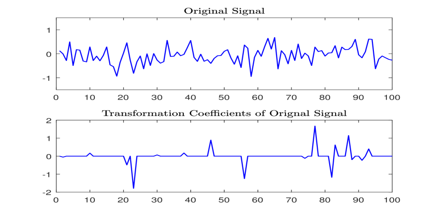
Figure 1: Original signal and its transformation coefficients. Upper: the original signal, which is density (not sparse); Down: the coefficients under tight frame transformation, which is sparse.

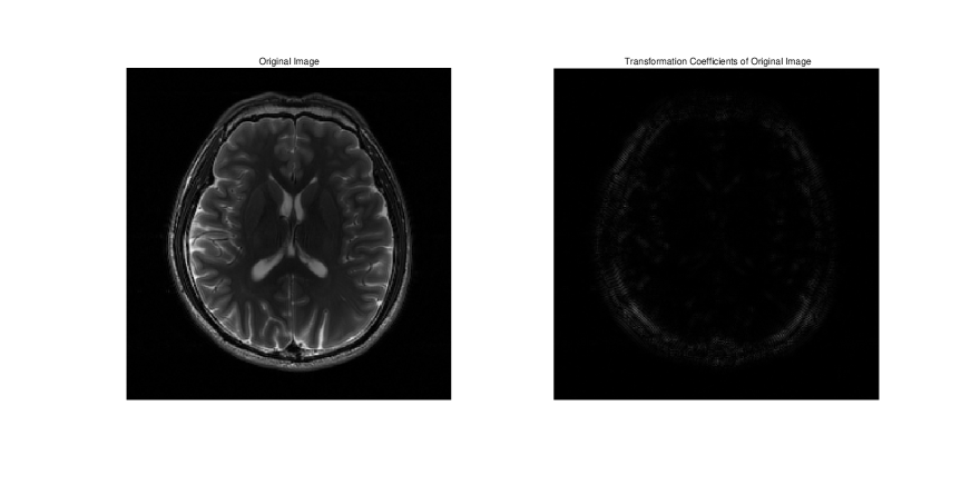
Figure 2: Brain MRI and its transformation coefficients. Left: the original Brain MRI, which is density (not sparse); Right: the coefficients under tight frame transformation, which is sparse. Here the black and white colors denote the pixel value $0$ and $1$, respectively.

1.3 Contributions

In this paper, we introduce the unconstrained $\ell_{1}-\alpha\ell_{2}$-analysis minimization:

$$\min_{\bm{x}\in\mathbb{R}^{n}}~{}\lambda(\|\bm{D}^{\top}\bm{x}\|_{1}-\alpha\|\bm{D}^{\top}\bm{x}\|_{2})+\frac{1}{2}\|\bm{Ax}-\bm{b}\|_{2}^{2}$$ (1.5)

for some constant $0<\alpha\leq 1$, where $\lambda$ is a regularization parameter. Denote (1.5) as Analysis $\ell_{1}-\alpha\ell_{2}$-Shrinkage and Selector Operator ($\ell_{1}-\alpha\ell_{2}$-ASSO). It is rooted to the sparse signal under tight frame and the constrained and unconstrained $\|\bm{x}\|_{1}-\alpha\|\bm{x}\|_{2}$ minimizations, which has recently attracted a lot of attention. The constrained $\|\bm{x}\|_{1}-\alpha\|\bm{x}\|_{2}$ minimization [28, 18, 33, 36, 37, 52] is

$$\min_{\bm{x}\in\mathbb{R}^{n}}~{}\|\bm{x}\|_{1}-\alpha\|\bm{x}\|_{2}\quad\text{subject \ to}\quad\bm{b}-\bm{A}\bm{x}\in\mathcal{B}.$$ (1.6)

And they have been introduced and studied different conditions based on RIP for the recovery of $\bm{x}$. The unconstrained $\|\bm{x}\|_{1}-\alpha\|\bm{x}\|_{2}$ minimization [33, 36, 37, 52, 19] is

$$\min_{\bm{x}\in\mathbb{R}^{n}}~{}\lambda(\|\bm{x}\|_{1}-\|\bm{x}\|_{2})+\frac{1}{2}\|\bm{A}\bm{x}-\bm{b}\|_{2}^{2}.$$ (1.7)

It is a key bridge for finding the solution of the constrained $\|\bm{x}\|_{1}-\alpha\|\bm{x}\|_{2}$ minimization (1.1). There is an effective algorithm based on the different of convex algorithm (DCA) to solve (1.7), see [37, 52]. Numerical examples in [28, 18, 37, 52] demonstrate that the $\ell_{1}-\alpha\ell_{2}$ minimization consistently outperforms the $\ell_{1}$ minimization and the $\ell_{p}$ minimization in [25] when the measurement matrix $\bm{A}$ is highly coherent.

Motivated by the smoothing and decomposition transformations in [47], the $\ell_{1}-\alpha\ell_{2}$-ASSO is written as a general nonsmooth convex optimization problem:

$$\min_{\bm{x}\in\mathbb{R}^{n}}~{}\lambda(\|\bm{z}\|_{1}-\alpha\|\bm{z}\|_{2})+\frac{1}{2}\|\bm{Ax}-\bm{b}\|_{2}^{2}+\frac{\rho}{2}\|\bm{D}^{\top}\bm{x}-\bm{z}\|_{2}^{2}.$$ (1.8)

We refer to it as Relaxed Analysis $\ell_{1}-\alpha\ell_{2}$-Shrinkage and Selector Operator ($\ell_{1}-\alpha\ell_{2}$-RASSO).

The main contributions are as follows:

1. We develop a new elementary technique for tight frames (Propositions 1 and 2) and show sufficient conditions based on $\bm{D}$-RIP and $\bm{D}$-ROC for the recovery of $\bm{x}$ from (1.1) via the $\ell_{1}-\alpha\ell_{2}$-ASSO (1.5), see to Theorem 1.

2. We show sufficient conditions based on $\bm{D}$-RIP frame for the recovery of the signal $\bm{x}$ from (1.1) via the $\ell_{1}-\alpha\ell_{2}$-RASSO (1.8), see to Theorem 2.

3. In order to find the solution of (1.5), we proposed an algorithm based on ADMM, which offers a noticeable boost to some sparse reconstruction algorithms for tight frames. Numerical examples based the effective algorithm is presented for both sparse signals and MRI. The recovery performance of the propose method is highly comparable (often better) to existing state-of-the-art methods.

1.4 Notations and Organization

Throughout the paper, we use the following basic notations. For any positive integer $n$, let $[[1,n]]$ be the set $\{1,\ldots,n\}$. For the index set $S\subseteq[[1,n]]$, let $|S|$ be the number of entries in $S$, $\bm{x}_{S}$ be the vector equal to $\bm{x}$ on $S$ and to zero on $S^{c}$, and $\bm{D}_{S}$ be $\bm{D}$ with all but the columns indexed by $S$ set to zero vector. For $\bm{x}\in\mathbb{R}^{n}$, denote $\bm{x}_{\max(s)}$ as the vector $\bm{x}$ with all but the largest $s$ entries in absolute value set to zero, and $\bm{x}_{-\max(s)}=\bm{x}-\bm{x}_{\max(s)}$. Let $\|\bm{D}^{\top}\bm{x}\|_{\alpha,1-2}$ be $\|\bm{D}^{\top}\bm{x}\|_{1}-\alpha\|\bm{D}^{\top}\bm{x}\|_{2}$. Especially, when $\alpha=1$, denote $\|\bm{D}^{\top}\bm{x}\|_{\alpha,1-2}$ with $\|\bm{D}^{\top}\bm{x}\|_{1-2}$. And we denote $n\times n$ identity matrix by $\bm{I}_{n}$, zeros matrix by $\bm{O}$, and the transpose of matrix $\bm{A}$ by $\bm{A}^{\top}$. Use the phrase “$s$-sparse vector” to refer to vectors of sparsity at most $s$. We use boldfaced letter to denote matrix or vector. We denote the standard inner product and Euclidean norm $\langle\cdot,\cdot\rangle$ and $\|\cdot\|_{2}$, respectively.

The rest of the paper is organized as follows. In Section 2, we describe some preliminaries about the tight frame and the unconstraint $\ell_{1}-\alpha\ell_{2}$ analysis models. In Section 3, we give the main conclusions and show their proof. Then we design an algorithm based on projected PISTA to solve the proposed model (1.5) in Section 4. And we also apply our algorithm to solve the proposed model for signal and MRI reconstruction in Section 5. Conclusions are given in Section 6.

2 Preliminaries

In this section, we first recall some significant lemmas in order to analyse the $\ell_{1}-\alpha\ell_{2}$-ASSO (1.5) and $\ell_{1}-\alpha\ell_{2}$-RASSO (1.8).

In view of the above-mentioned facts in Section 1, the $\bm{D}$-RIP plays a key role for the stable recovery of signal via the analysis approach. The following lemma show some basic properties in [32] for the $\bm{D}$-RIP with $\delta_{s}$ and $\theta_{s,t}$.

Lemma 1.

1. For any $s_{1}\leq s_{2}\leq d$, we have $\delta_{s_{1}}\leq\delta_{s_{2}}$.

2. For any positive integers $s$ and $t_{1}\leq t_{2}$, we have $\theta_{s,t_{2}}\leq\sqrt{\frac{t_{2}}{t_{1}}}\theta_{s,t_{1}}$.

3. $\theta_{s_{1},t_{1}}\leq\theta_{s_{2},t_{2}}$ if $s_{1}\leq s_{2}$ and $t_{1}\leq t_{2}$ with $s_{2}+t_{2}\leq d$.

4. For all nonnegative integers $s,t\leq d$, we have $\theta_{s,t}\leq\delta_{s+t}$.

Here, we proposed the standard properties for the dictionary $\bm{D}$.

Proposition 1.

Let $\bar{\bm{D}}\in\mathbb{R}^{(d-n)\times d}$ be the orthogonal complement of $\bm{D}\in\mathbb{R}^{n\times d}$, i.e., $\bar{\bm{D}}\bm{D}^{\top}=\bm{0}$, $\bar{\bm{D}}\bar{\bm{D}}^{\top}=\bm{I}_{n-d}$. Then,

1. For any $\bm{v}\in\mathbb{R}^{d}$, $\|\bm{v}\|_{2}^{2}=\|\bm{Dv}\|_{2}^{2}+\|\bar{\bm{D}}\bm{v}\|_{2}^{2}$.

2. For any $s$-sparse signal $\bm{v}\in\mathbb{R}^{d}$, we have

   $$(1-\delta_{s})\|\bm{v}\|_{2}^{2}\leq\|\bm{A}\bm{Dv}\|_{2}^{2}+\|\bar{\bm{D}}\bm{v}\|_{2}^{2}\leq(1+\delta_{s})\|\bm{v}\|_{2}^{2}.$$

3. $\langle\bm{u},\bm{v}\rangle=\langle\bar{\bm{D}}\bm{u},\bar{\bm{D}}\bm{v}\rangle+\langle\bm{D}\bm{u},\bm{D}\bm{v}\rangle$ for any $\bm{u}\in\mathbb{R}^{d}$.

4. For any $\|\bm{u}\|_{0}\leq s$ and $\|\bm{v}\|_{0}\leq t$, we have

   $$|\langle\bm{A}\bm{Du},\bm{A}\bm{Dv}\rangle+\langle\bar{\bm{D}}\bm{u},\bar{\bm{D}}\bm{v}\rangle-\langle\bm{u},\bm{v}\rangle|\leq\theta_{s,t}\|\bm{u}\|_{2}\|\bm{v}\|_{2}.$$

   Moreover, if $\text{\rm supp}(\bm{u})\cap\text{\rm supp}(\bm{v})=\emptyset$, we have

   $$|\langle\bm{A}\bm{Du},\bm{A}\bm{Dv}\rangle+\langle\bar{\bm{D}}\bm{u},\bar{\bm{D}}\bm{v}\rangle|\leq\theta_{s,t}\|\bm{u}\|_{2}\|\bm{v}\|_{2}.$$

Proof.

Despite the results $(i)$ and $(ii)$ in Proposition 1 are clear, we here give their proofs. As far as we know, the results (iii) and (iv) are first proved.

$(i)$ For any $v\in\mathbb{R}^{d}$, there is

$$\|\bm{Dv}\|_{2}^{2}+\|\bar{\bm{D}}\bm{v}\|_{2}^{2} =\langle\bm{D}^{\top}\bm{D}\bm{v},\bm{v}\rangle+\langle\bar{\bm{D}}^{\top}\bar{\bm{D}}\bm{v},\bm{v}\rangle$$

$$=\bm{v}^{\top}\begin{bmatrix}\bm{D}^{\top}&\bar{\bm{D}}^{\top}\\ \end{bmatrix}\begin{bmatrix}\bm{D}\\ \bar{\bm{D}}\\ \end{bmatrix}\bm{v}=\|\bm{v}\|_{2}^{2},$$

where the last equality comes from the definition of tight frame $\bm{D}\bm{D}^{\top}=\bm{I}_{n}$ and the definition of the orthogonal complement of frame $\bar{\bm{D}}\bar{\bm{D}}^{\top}=\bm{I}_{n-d}$.

$(ii)$ By the definition of $\bm{D}$-RIP, we have

$$\|\bm{A}\bm{Dv}\|_{2}^{2}+\|\bar{\bm{D}}\bm{v}\|_{2}^{2} \leq(1+\delta_{s})\|\bm{Dv}\|_{2}^{2}+\|\bar{\bm{D}}\bm{v}\|_{2}^{2}\leq(1+\delta_{s})\left(\|\bm{Dv}\|_{2}^{2}+\|\bar{\bm{D}}\bm{v}\|_{2}^{2}\right)$$

$$=(1+\delta_{s})\|\bm{v}\|_{2}^{2},$$ (2.1)

where the equality comes from the item $(i)$. Similarly, we can show the lower bound

$$\|\bm{A}\bm{Dv}\|_{2}^{2}+\|\bar{\bm{D}}\bm{v}\|_{2}^{2}\geq(1-\delta_{s})\|\bm{v}\|_{2}^{2}.$$ (2.2)

The combination of the upper bound (2) and the lower bound (2.2) gives the item (ii).

Next, we show our new conclusions items (iii) and (iv).

$(iii)$ According to the parallelogram identity, we have

$$\langle\bar{\bm{D}}\bm{u},\bar{\bm{D}}\bm{v}\rangle =\frac{1}{4}\left(\|\bar{\bm{D}}(\bm{u}+\bm{v})\|_{2}^{2}-\|\bar{\bm{D}}(\bm{u}-\bm{v})\|_{2}^{2}\right),$$

$$\langle\bm{D}\bm{u},\bm{D}\bm{v}\rangle =\frac{1}{4}\left(\|\bm{D}(\bm{u}+\bm{v})\|_{2}^{2}-\|\bm{D}(\bm{u}-\bm{v})\|_{2}^{2}\right).$$

Taking sum over both side of above two equalities, one has

$$\langle\bar{\bm{D}}\bm{u},\bar{\bm{D}}\bm{v}\rangle+\langle\bm{D}\bm{u},\bm{D}\bm{v}\rangle$$

$$=\frac{1}{4}\left(\left(\|\bar{\bm{D}}(\bm{u}+\bm{v})\|_{2}^{2}+\|\bm{D}(\bm{u}+\bm{v})\|_{2}^{2}\right)-\left(\|\bar{\bm{D}}(\bm{u}-\bm{v})\|_{2}^{2}+\|\bm{D}(\bm{u}-\bm{v})\|_{2}^{2}\right)\right)$$

$$=\frac{1}{4}\left(\|\bm{u}+\bm{v}\|_{2}^{2}-\|\bm{u}-\bm{v}\|_{2}^{2}\right),$$ (2.3)

where the second equality holds because of the item $(i)$. Last, by the above (2) and the following parallelogram identity

$$\langle\bm{u},\bm{v}\rangle=\frac{1}{4}\left(\|(\bm{u}+\bm{v})\|_{2}^{2}-\|(\bm{u}-\bm{v})\|_{2}^{2}\right),$$

we get

$$\langle\bm{u},\bm{v}\rangle=\langle\bar{\bm{D}}\bm{u},\bar{\bm{D}}\bm{v}\rangle+\langle\bm{D}\bm{u},\bm{D}\bm{v}\rangle.$$

$(iv)$ It follows from the item $(ii)$ and the definition of $\bm{D}$-ROC that

$$|\langle\bm{A}\bm{Du},\bm{A}\bm{Dv}\rangle+\langle\bar{\bm{D}}\bm{u},\bar{\bm{D}}\bm{v}\rangle-\langle\bm{u},\bm{v}\rangle|=|\langle\bm{A}\bm{Du},\bm{A}\bm{Dv}\rangle-\langle\bm{D}\bm{u},\bm{D}\bm{v}\rangle|nonumber$$

$$\leq\theta_{s,t}\|\bm{u}\|_{2}\|\bm{v}\|_{2},$$

which is our desired conclusion. ∎

Next, the following inequality is a modified cone constraint inequality for the unconstrained $\|\bm{D}^{\top}\bm{x}\|_{1}-\alpha\|\bm{D}^{\top}\bm{x}\|_{2}$ minimization (1.5). Its proof is similar as that of [19, Lemma 2.3] and we omit its proof.

Lemma 2.

Let $\bm{b}=\bm{Ax}+\bm{e}$ with $\|\bm{e}\|_{2}\leq\lambda$, $T=\text{\rm supp}(\bm{D}^{\top}\bm{x}_{\max(t)})$, and $\hat{\bm{x}}$ be a minimization solution of (1.5). Then

$$\|\bm{Ah}\|_{2}^{2}+2\lambda\|\bm{D}_{T^{c}}^{\top}\bm{h}\|_{1}\leq 2\lambda(\|\bm{D}_{T}^{\top}\bm{h}\|_{1}+\alpha\|\bm{D}^{\top}\bm{h}\|_{2}+2\|\bm{D}_{T^{c}}^{\top}\bm{x}\|_{1}+\|\bm{Ah}\|_{2}),$$ (2.4)

where ${\bm{h}}=\hat{{\bm{x}}}-{\bm{x}}$. And moreover,

$$\|\bm{Ah}\|_{2}^{2}+2\lambda(\|{\bm{D}}_{T^{c}}^{\top}{\bm{h}}\|_{1}-\alpha\|{\bm{D}}_{T^{c}}^{\top}{\bm{h}}\|_{2})\leq 2\lambda(\|{\bm{D}}_{T}^{\top}{\bm{h}}\|_{1}+2\|{\bm{D}}_{T^{c}}^{\top}{\bm{x}}\|_{1}+\alpha\|{\bm{D}}_{T}^{\top}{\bm{h}}\|_{2}+\|\bm{Ah}\|_{2}),$$

$$\|{\bm{D}}_{T^{c}}^{\top}{\bm{h}}\|_{1}\leq\|{\bm{D}}_{T}^{\top}{\bm{h}}\|_{1}+2\|{\bm{D}}_{T^{c}}^{\top}{\bm{x}}\|_{1}+\alpha\|{\bm{D}}^{\top}{\bm{h}}\|_{2}+\|\bm{Ah}\|_{2},$$

and

$$\|{\bm{A}h}\|_{2}^{2}\leq 2\lambda(\|{\bm{D}}_{T}^{\top}{\bm{h}}\|_{1}+2\|{\bm{D}}_{T^{c}}^{\top}{\bm{x}}\|_{1}+\alpha\|{\bm{D}}^{\top}{\bm{h}}\|_{2}+\|\bm{Ah}\|_{2}).$$

For the $\ell_{1}-\alpha\ell_{2}$-RASSO (1.8), there is a similar cone constraint inequality.

Lemma 3.

Let ${\bm{b}}={\bm{Ax}}+{\bm{e}}$ with $\|\bm{e}\|_{2}\leq\lambda$, and $T=\text{\rm supp}({\bm{D}}^{\top}{\bm{x}}_{\max(s)})$. Then the minimization solution $\hat{\bm{x}}$ of (1.8) satisfies

$$\|\bm{Ah}\|_{2}^{2}+2\lambda\|{\bm{D}}_{T^{c}}^{\top}{\bm{h}}\|_{1}\leq 2\lambda\bigg{(}\|{\bm{D}}_{T}^{\top}{\bm{h}}\|_{1}+\alpha\|{\bm{D}}^{\top}{\bm{h}}\|_{2}+2\|{\bm{D}}_{T^{c}}^{\top}{\bm{x}}\|_{1}+\|\bm{Ah}\|_{2}+\frac{(\alpha+1)^{2}d}{2}\frac{\lambda}{\rho}\bigg{)},$$ (2.5)

where ${\bm{h}}=\hat{{\bm{x}}}-{\bm{x}}$.

Proof.

Our proof is motivated by the proof of [19, Lemma 2.3] and [47, Lemma IV.4]. Assume that $(\hat{\bm{x}},\hat{\bm{z}})$ is another solution of (1.8), then

$$0 \geq\bigg{(}\lambda(\|\hat{{\bm{z}}}\|_{1}-\alpha\|\hat{{\bm{z}}}\|_{2})+\frac{1}{2}\|{\bm{A}}\hat{{\bm{x}}}-{\bm{b}}\|_{2}^{2}+\frac{\rho}{2}\|{\bm{D}}^{\top}\hat{{\bm{x}}}-\hat{{\bm{z}}}\|_{2}^{2}\bigg{)}$$

$$\hskip 12.0pt-\bigg{(}\lambda(\|{\bm{D}}^{\top}{\bm{x}}\|_{1}-\alpha\|{\bm{D}}^{\top}{\bm{x}}\|_{2})+\frac{1}{2}\|{\bm{A}}{\bm{x}}-{\bm{b}}\|_{2}^{2}\bigg{)}$$

$$=\frac{1}{2}\bigg{(}\|{\bm{A}}\hat{{\bm{x}}}-{\bm{b}}\|_{2}^{2}-\|{\bm{A}}{\bm{x}}-{\bm{b}}\|_{2}^{2}\bigg{)}$$

$$\hskip 12.0pt+\bigg{(}\lambda(\|\hat{{\bm{z}}}\|_{1}-\alpha\|\hat{{\bm{z}}}\|_{2})+\frac{\rho}{2}\|{\bm{D}}^{\top}\hat{{\bm{x}}}-\hat{{\bm{z}}}\|_{2}^{2}-\lambda(\|{\bm{D}}^{\top}{\bm{x}}\|_{1}-\alpha\|{\bm{D}}^{\top}{\bm{x}}\|_{2})\bigg{)}$$

$$=:I_{1}+I_{2}.$$ (2.6)

Next, we deal with terms $I_{1}$ and $I_{2}$, respectively. By $\hat{{\bm{x}}}={\bm{h}}+{\bm{x}}$ and ${\bm{A}x}-{\bm{b}}=-{\bm{e}}$,

$$I_{1} =\frac{1}{2}\bigg{(}\|{\bm{A}}{\bm{h}}-{\bm{e}}\|_{2}^{2}-\|-{\bm{e}}\|_{2}^{2}\bigg{)}=\frac{1}{2}\|{\bm{A}}{\bm{h}}\|_{2}^{2}-\langle{\bm{A}}{\bm{h}},{\bm{e}}\rangle$$

$$\overset{(1)}{\geq}\frac{1}{2}\|{\bm{A}}{\bm{h}}\|_{2}^{2}-\|{\bm{A}}{\bm{h}}\|_{2}\|{\bm{e}}\|_{2}\overset{(2)}{\geq}\frac{1}{2}\|{\bm{A}}{\bm{h}}\|_{2}^{2}-\lambda\|{\bm{A}}{\bm{h}}\|_{2},$$ (2.7)

where the inequality (1) comes from the Cauchy-Schwarz inequality, and the inequality (2) is from $\|{\bm{e}}\|_{2}\leq\lambda$.

Then, we estimate the term $I_{2}$. The subgradient optimality condition for (1.8) is

$${\bm{0}} ={\bm{A}}^{\top}({\bm{A}}\hat{{\bm{x}}}-{\bm{b}})+\rho{\bm{D}}({\bm{D}}^{\top}\hat{{\bm{x}}}-\hat{{\bm{z}}}),$$

$${\bm{0}} \in\lambda{\bm{v}}-\rho({\bm{D}}^{\top}\hat{{\bm{x}}}-\hat{{\bm{z}}}),$$

where ${\bm{v}}$ is a Frech$\acute{e}$t sub-differential of the function $\|\hat{{\bm{z}}}\|_{1}-\alpha\|\hat{{\bm{z}}}\|_{2}$. Then, we derive that

$$I_{2} =\lambda(\|\hat{{\bm{z}}}\|_{1}-\|{\bm{D}}^{\top}{\bm{x}}\|_{1})-\lambda\alpha(\|\hat{{\bm{z}}}\|_{2}-\|{\bm{D}}^{\top}{\bm{x}}\|_{2})+\frac{\rho}{2}\|{\bm{D}}^{\top}\hat{{\bm{x}}}-\hat{{\bm{z}}}\|_{2}^{2}$$

$$=\lambda\left(\left\|{\bm{D}}^{\top}\hat{{\bm{x}}}-\frac{\lambda}{\rho}{\bm{v}}\right\|_{1}-\|{\bm{D}}^{\top}{\bm{x}}\|_{1}\right)-\lambda\alpha\left(\left\|{\bm{D}}^{\top}\hat{{\bm{x}}}-\frac{\lambda}{\rho}{\bm{v}}\right\|_{2}-\|{\bm{D}}^{\top}{\bm{x}}\|_{2}\right)+\frac{\rho}{2}\|\frac{\lambda}{\rho}{\bm{v}}\|_{2}^{2}$$

$$\overset{(a)}{\geq}\lambda\left(\|{\bm{D}}^{\top}\hat{{\bm{x}}}\|_{1}-\|{\bm{D}}^{\top}{\bm{x}}\|_{1}-\frac{\lambda}{\rho}\|{\bm{v}}\|_{1}\right)-\lambda\alpha\left(\|{\bm{D}}^{\top}\hat{{\bm{x}}}\|_{2}-\|{\bm{D}}^{\top}{\bm{x}}\|_{2}+\frac{\lambda}{\rho}\|{\bm{v}}\|_{2}\right)+\frac{\lambda^{2}}{2\rho}\|{\bm{v}}\|_{2}^{2}$$

$$=\lambda\left(\left(\|{\bm{D}}^{\top}\hat{{\bm{x}}}\|_{1}-\|{\bm{D}}^{\top}{\bm{x}}\|_{1}\right)-\alpha\left(\|{\bm{D}}^{\top}\hat{{\bm{x}}}\|_{2}-\|{\bm{D}}^{\top}{\bm{x}}\|_{2}\right)\right)$$

$$\hskip 12.0pt+\frac{\lambda^{2}}{2\rho}(\|{\bm{v}}\|_{2}^{2}-2\|{\bm{v}}\|_{1}-2\alpha\|{\bm{v}}\|_{2})$$

$$=:I_{21}+I_{22},$$ (2.8)

where (a) is because of $\|{\bm{u}}\|_{p}-\|{\bm{v}}\|_{p}\leq\|\bm{u+v}\|_{p}\leq\|{\bm{u}}\|_{p}+\|{\bm{v}}\|_{p}$ for any $1\leq p\leq\infty$. Note that

$$I_{21} =\lambda\left(\|{\bm{D}}_{T}^{\top}(\bm{h+x})+{\bm{D}}_{T^{c}}^{\top}(\bm{h+x})\|_{1}-\|{\bm{D}}_{T}^{\top}{\bm{x}}+{\bm{D}}_{T^{c}}^{\top}{\bm{x}}\|_{1}\right)$$

$$\hskip 12.0pt-\lambda\alpha\left(\|{\bm{D}}^{\top}(\bm{h+x})\|_{2}-\|{\bm{D}}^{\top}{\bm{x}}\|_{2}\right)$$

$$\geq\lambda\left(\|{\bm{D}}_{T}^{\top}{\bm{x}}\|_{1}-\|{\bm{D}}_{T}^{\top}{\bm{h}}\|_{1}+\|{\bm{D}}_{T^{c}}^{\top}{\bm{h}}\|_{1}-\|{\bm{D}}_{T^{c}}^{\top}{\bm{x}}\|_{1}-\|{\bm{D}}_{T}^{\top}{\bm{x}}\|_{1}-\|{\bm{D}}_{T^{c}}^{\top}{\bm{x}}\|_{1}\right)$$

$$\hskip 12.0pt-\lambda\alpha\left(\|{\bm{D}}^{\top}{\bm{h}}\|_{2}\right)$$

$$=\lambda(\|{\bm{D}}_{T^{c}}^{\top}{\bm{h}}\|_{1}-\|{\bm{D}}_{T}^{\top}{\bm{h}}\|_{1}-2\|{\bm{D}}_{T^{c}}^{\top}{\bm{x}}\|_{1}-\alpha\|{\bm{D}}^{\top}{\bm{h}}\|_{2}),$$ (2.9)

where the inequality is because of $\|\bm{u+v}\|_{1}\geq\|{\bm{u}}\|_{1}-\|{\bm{v}}\|_{1}$ and $\|\bm{u+v}\|_{1}\leq\|{\bm{u}}\|_{1}+\|{\bm{v}}\|_{1}$. On the other hand,

$$I_{22} \overset{(1)}{\geq}\frac{\lambda^{2}}{2\rho}\left(\|{\bm{v}}\|_{2}^{2}-2(1+\alpha)\|{\bm{v}}\|_{1}\right)$$

$$=\frac{\lambda^{2}}{2\rho}\sum_{j=1}^{d}\left((|v|_{j}-(1+\alpha))^{2}-(1+\alpha)^{2}\right)\overset{(2)}{\geq}-\frac{(1+\alpha)^{2}\lambda^{2}d}{2\rho},$$ (2.10)

where (1) is because of $\|{\bm{v}}\|_{2}\leq\|{\bm{v}}\|_{1}$, and the equality (2) holds if and only if $|v|_{j}=(1+\alpha)$ for all $j=1,\ldots,d$. Substituting the estimate (2) and (2) into (2), one has

$$I_{2}\geq\lambda\left(\|{\bm{D}}_{T^{c}}^{\top}{\bm{h}}\|_{1}-\|{\bm{D}}_{T}^{\top}{\bm{h}}\|_{1}-2\|{\bm{D}}_{T^{c}}^{\top}{\bm{x}}\|_{1}-\alpha\|{\bm{D}}^{\top}{\bm{h}}\|_{2}-\frac{(1+\alpha)^{2}d\lambda}{2\rho}\right).$$ (2.11)

Last, substituting the estimate of $I_{1}$ in (2) and $I_{2}$ in (2.11) into the inequality (2), we get (2.5). ∎

The following lemma is the fundamental properties of the metric $\|{\bm{x}}\|_{1}-\alpha\|{\bm{x}}\|_{2}$ with $0\leq\alpha\leq 1$, see [52] and [18].

Lemma 4.

For any $\bm{x}\in\mathbb{R}^{n}$, the following statements hold:

(a) Let $0\leq\alpha\leq 1$, $T=\text{\rm supp}({\bm{x}})$ and $\|{\bm{x}}\|_{0}=s$. Then

$$(s-\alpha\sqrt{s})\min_{j\in T}|x_{j}|\leq\|{\bm{x}}\|_{1}-\alpha\|{\bm{x}}\|_{2}\leq(\sqrt{s}-\alpha)\|{\bm{x}}\|_{2}.$$ (2.12)

(b) Let $S,S_{1},S_{2}\subseteq[n]$ satisfy $S=S_{1}\cup S_{2}$ and $S_{1}\cap S_{2}=\emptyset$. Then

$$\|\bm{x}_{S_{1}}\|_{1}-\alpha\|\bm{x}_{S_{1}}\|_{2}+\|\bm{x}_{S_{2}}\|_{1}-\alpha\|\bm{x}_{S_{2}}\|_{2}\leq\|\bm{x}_{S}\|_{1}-\alpha\|\bm{x}_{S}\|_{2}.$$ (2.13)

Now, we can give the key technical tool used in the main results. It provides an estimation based on $\bm{D}$-ROC for $|\langle\bm{ADu},\bm{ADv}\rangle+\langle\bar{{\bm{D}}}{\bm{u}},\bar{{\bm{D}}}{\bm{v}}\rangle|$, where one of $\bm{u}$ or $\bm{v}$ is sparse. Our idea is inspired by [6, Lemma 5.1] and [27, Lemma 2.3].

Proposition 2.

Let $s_{1},s_{2}\leq n$. Suppose ${\bm{u}},{\bm{v}}\in\mathbb{R}^{d}$ satisfy $\text{\rm supp}({\bm{u}})\cap\text{\rm supp}({\bm{v}})=\emptyset$ and $\bm{u}$ is $s_{1}$ sparse. If $\|{\bm{v}}\|_{1-2}\leq(s_{2}-\sqrt{s_{2}})\eta$ and $\|{\bm{v}}\|_{\infty}\leq\eta$, then

$$|\langle\bm{ADu},\bm{ADv}\rangle+\langle\bar{{\bm{D}}}{\bm{u}},\bar{{\bm{D}}}{\bm{v}}\rangle|\leq\bigg{(}1+\frac{\sqrt{2}}{2}\bigg{)}\eta\sqrt{s_{2}}\theta_{s_{1},s_{2}}\|\bm{u}\|_{2}.$$ (2.14)

Before giving the proof of Proposition 2, we first recall a convex combination of sparse vectors for any point based on the metric $\|\cdot\|_{1}-\|\cdot\|_{2}$.

Lemma 5.

[17, Lemma2.2] Let a vector $\bm{\nu}\in\mathbb{R}^{d}$ satisfy $\|\bm{\nu}\|_{\infty}\leq\eta$, where $\alpha$ is a positive constant. Suppose $\|\bm{\nu}\|_{1-2}\leq(s-\sqrt{s})\eta$ with a positive integer $s$ and $s\leq|\mathrm{supp}(\bm{\nu})|$. Then $\bm{\nu}$ can be represented as a convex combination of $s$-sparse vectors $\bm{v}^{(i)}$, i.e.,

$$\bm{\nu}=\sum_{i=1}^{N}\lambda_{i}\bm{v}^{(i)},$$ (2.15)

where $N$ is a positive integer,

$$0<\lambda_{i}\leq 1,\ \ \ \ \sum_{i=1}^{N}\lambda_{i}=1,$$ (2.16)

$$\mathrm{supp}(\bm{v}^{(i)})\subseteq\mathrm{supp}(\bm{\nu}),\ \ \|\bm{v}^{(i)}\|_{0}\leq{s},\ \ \|\bm{v}^{(i)}\|_{\infty}\leq\Big{(}1+\frac{\sqrt{2}}{2}\Big{)}\eta,$$ (2.17)

and

$$\sum_{i=1}^{N}\lambda_{i}\|\bm{v}^{(i)}\|_{2}^{2}\leq\Big{[}\Big{(}1+\frac{\sqrt{2}}{2}\Big{)}^{2}(s-\sqrt{s})+1\Big{]}\theta^{2}.$$ (2.18)

Now, we give the proof of Proposition 2 in details.

Proof.

Suppose $\|\bm{v}\|_{0}=t$. We consider two cases as follows.

Case I: $t\leq s_{2}$.

By the item (iv) of Proposition 1 and $\|{\bm{v}}\|_{\infty}\leq\alpha$, we have

$$|\langle\bm{ADu},\bm{ADv}\rangle+\langle\bar{{\bm{D}}}{\bm{u}},\bar{{\bm{D}}}{\bm{v}}\rangle| \leq\theta_{s_{1},t}\|{\bm{u}}\|_{2}\|{\bm{v}}\|_{2}\leq\theta_{s_{1},t}\|{\bm{u}}\|_{2}\|{\bm{v}}\|_{\infty}\sqrt{\|{\bm{v}}\|_{0}}$$

$$\leq\eta\sqrt{s_{2}}\theta_{s_{1},s_{2}}\|{\bm{u}}\|_{2}.$$ (2.19)

Case II: $t>s_{2}$.

We shall prove by induction. Assume that (2.14) holds for $t-1$. Note that $\|{\bm{v}}\|_{1-2}\leq\eta(s_{2}-\sqrt{s_{2}})$ and $\|{\bm{v}}\|_{\infty}\leq\eta$. By Lemma 5, ${\bm{v}}$ can be represented as the convex hull of $s_{2}$-sparse vectors:

$${\bm{v}}=\sum_{j=1}^{N}\gamma_{j}{\bm{v}}^{j},$$

where ${\bm{v}}^{j}$ is $s_{2}$-sparse for any $j\in[N]$ and

$$\sum_{j=1}^{N}\gamma_{j}=1,~{}~{}0<\gamma_{j}\leq 1,j\in[N].$$

Since $\bm{v}^{j}$ is $s_{2}$-sparse and $s_{2}\leq t-1$, we use the induction assumption,

$$|\langle\bm{ADu},\bm{ADv}\rangle+\langle\bar{{\bm{D}}}{\bm{u}},\bar{{\bm{D}}}{\bm{v}}\rangle|\leq\sum_{j=1}^{N}\gamma_{j}|\langle\bm{ADu},\bm{AD}\bm{v}^{j}\rangle+\langle\bar{{\bm{D}}}{\bm{u}},\bar{{\bm{D}}}{\bm{v}}^{j}\rangle|$$

$$\overset{(a)}{\leq}\sum_{j=1}^{N}\gamma_{j}\bigg{(}\theta_{s_{1},s_{2}}\|\bm{v}^{j}\|_{2}\|\bm{u}\|_{2}\bigg{)}\leq\sum_{j=1}^{N}\gamma_{j}\bigg{(}\theta_{s_{1},s_{2}}\|\bm{v}^{j}\|_{\infty}\sqrt{\|\bm{v}^{j}\|_{0}}\|\bm{u}\|_{2}\bigg{)}$$

$$\overset{(b)}{\leq}\sum_{j=1}^{N}\gamma_{j}\bigg{(}\bigg{(}1+\frac{\sqrt{2}}{2}\bigg{)}\eta\sqrt{s_{2}}\theta_{s_{1},s_{2}}\|\bm{u}\|_{2}\bigg{)}=\bigg{(}1+\frac{\sqrt{2}}{2}\bigg{)}\eta\sqrt{s_{2}}\theta_{s_{1},s_{2}}\|\bm{u}\|_{2},$$ (2.20)

where (a) is in view of the item (iv) of Proposition 1, and (b) is in virtue of Lemma 5.

The combination of Case I and Case II is (2.14). ∎

3 Main Result based on D-RIC and D-ROC

In this section, we develop sufficient conditions based on $\bm{D}$-RIC and $\bm{D}$-ROC of the $\ell_{1}-\alpha\ell_{2}$-ASSO (1.5) and $\ell_{1}-\alpha\ell_{2}$-RASSO (1.8) for the signal recovery applying the technique of the convex combination.

3.1 Auxiliary Lemmas Under RIP Frame

Combining the above auxiliary results in Section 2, we first introduce some main inequalities, which play an important role in establishing the recovery condition of the $\ell_{1}-\alpha\ell_{2}$-ASSO (1.5) and $\ell_{1}-\alpha\ell_{2}$-RASSO (1.8).

Proposition 3.

For positive integers $s\geq 2$ and $k\geq 1$, let $S=\text{\rm supp}({\bm{D}}^{\top}{\bm{h}}_{\max(s)})$ and $T=\text{\rm supp}({\bm{D}}^{\top}{\bm{x}}_{\max(s)})$. Assume that

$$\|\bm{D}_{S^{c}}^{\top}\bm{h}\|_{1}-\alpha\|\bm{D}_{S^{c}}^{\top}\bm{h}\|_{2}\leq a\|\bm{D}_{S}^{\top}\bm{h}\|_{1}+b\|\bm{D}_{S}^{\top}\bm{h}\|_{2}+c\|\bm{D}_{T^{c}}^{\top}\bm{x}\|_{1}+\eta\|{\bm{Ah}}\|_{2}+\gamma,$$ (3.1)

where $a>0$ and $b,c,\eta,\gamma\geq 0$ satisfy $(a-1)\sqrt{s}+(b+1)\geq 0$. Then the following statements hold:

(i)

For the set $S$, one has

$$|\langle\bm{AD}\bm{D}_{S}^{\top}{\bm{h}},\bm{AD}\bm{D}_{S^{c}}^{\top}{\bm{h}}\rangle|$$

$$\leq\theta_{s,s}\sqrt{s}\Big{(}1+\frac{\sqrt{2}}{2}\Big{)}\Big{(}\frac{a\sqrt{s}+b}{\sqrt{s}-1}\frac{\|\bm{D}_{S}^{\top}\bm{h}\|_{2}}{\sqrt{s}}+\frac{c\|\bm{D}_{T^{c}}^{\top}\bm{x}\|_{1}+\eta\|{\bm{A}h}\|_{2}+\gamma}{s-\sqrt{s}}\Big{)}\|\bm{D}_{S}^{\top}{\bm{h}}\|_{2},$$ (3.2)

(ii)

Let the set

$$\tilde{S}=S\cup\Big{\{}i:|(\bm{D}_{S^{c}}^{\top}\bm{h})(i)|>\frac{1}{t-1}\frac{a\sqrt{s}+b}{\sqrt{s}-1}\frac{\|\bm{D}_{S}^{\top}\bm{h}\|_{2}}{\sqrt{s}}+\frac{c\|\bm{D}_{T^{c}}^{\top}\bm{x}\|_{1}+\eta\|{\bm{A}h}\|_{2}+\gamma}{(t-1)(s-\sqrt{s})}\Big{\}}$$ (3.3)

for any $t>3$. Then

$$|\langle\bm{AD}\bm{D}_{\tilde{S}}^{\top}{\bm{h}},\bm{AD}\bm{D}_{\tilde{S}^{c}}^{\top}{\bm{h}}\rangle|\leq\theta_{ts,(t-1)s}\frac{\sqrt{\lceil(t-1)s\rceil}}{t-1}\Big{(}1+\frac{\sqrt{2}}{2}\Big{)}$$

$$\times\Big{(}\frac{a\sqrt{s}+b}{\sqrt{s}-1}\frac{\|\bm{D}_{S}^{\top}\bm{h}\|_{2}}{\sqrt{s}}+\frac{c\|\bm{D}_{T^{c}}^{\top}\bm{x}\|_{1}+\eta\|{\bm{A}h}\|_{2}+\gamma}{s-\sqrt{s}}\Big{)}\|\bm{D}_{\tilde{S}}^{\top}{\bm{h}}\|_{2}.$$ (3.4)

(iii)

Let $\bm{A}$ satisfy $\bm{D}$-RIP with

$$\rho_{s,t}=:\delta_{ts}+\sqrt{\frac{\lceil(t-1)s\rceil}{(t-1)^{2}s}}\frac{(\sqrt{2}+1)(\sqrt{s}+\alpha)}{\sqrt{2}(\sqrt{s}-1)}\theta_{st,(t-1)s}<1,$$ (3.5)

with $t\geq 3$. Then

$$\|\bm{D}_{S}^{\top}\bm{h}\|_{2}\leq \frac{(\sqrt{2}+1)\theta_{ts,(t-1)s}}{\sqrt{2}(1-\rho_{s,t})}\frac{\sqrt{\lceil(t-1)s\rceil}}{(t-1)(s-\sqrt{s})}\Big{(}c\|\bm{D}_{T^{c}}^{\top}\bm{x}\|_{1}+\gamma\Big{)}$$

$$+\Big{(}\frac{(\sqrt{2}+1)\theta_{ts,(t-1)s}}{\sqrt{2}(1-\rho_{s,t})}\frac{\sqrt{(t-1)s}}{(t-1)(s-\sqrt{s})}+\frac{\sqrt{1+\delta_{ts}}}{1-\rho_{s,t}}\Big{)}\eta\|\bm{Ah}\|_{2},$$ (3.6)

where $\eta\geq 1$.

(iv)

Let $\bm{A}$ satisfy $\bm{D}$-RIP with

$$\rho_{s}=:\delta_{s}+\frac{(\sqrt{2}+1)(\sqrt{s}+\alpha)}{\sqrt{2}(\sqrt{s}-1)}\theta_{s,s}<1.$$ (3.7)

Then

$$\|\bm{D}_{S}^{\top}\bm{h}\|_{2}\leq \frac{(\sqrt{2}+1)\theta_{s,s}}{\sqrt{2}(1-\rho_{s})(\sqrt{s}-1)}\Big{(}c\|\bm{D}_{T^{c}}^{\top}\bm{x}\|_{1}+\gamma\Big{)}$$

$$+\Big{(}\frac{(\sqrt{2}+1)\theta_{s,s}}{\sqrt{2}(1-\rho_{s})(\sqrt{s}-1)}+\frac{\sqrt{1+\delta_{s}}}{1-\rho_{s}}\Big{)}\eta\|\bm{Ah}\|_{2},$$ (3.8)

where $\eta\geq 1$.

(v)

For the term $\|\bm{D}_{S^{c}}^{\top}\bm{h}\|_{2}$, there is

$$\|\bm{D}_{S^{c}}^{\top}\bm{h}\|_{2}$$

$$\leq\Bigg{(}\sqrt{\frac{a\sqrt{s}+b}{\sqrt{s}}+\frac{\alpha^{2}}{4s}}+\frac{\alpha+\bar{\varepsilon}}{2\sqrt{s}}\Bigg{)}\|\bm{D}_{S}^{\top}\bm{h}\|_{2}+\frac{1}{2\bar{\varepsilon}}\big{(}c\|\bm{D}_{T^{c}}^{\top}\bm{x}\|_{1}+\eta\|\bm{Ah}\|_{2}+\gamma\big{)},$$ (3.9)

where $\bar{\varepsilon}>0$ is a constant.

Proof.

Please see Appendix A. ∎

3.2 Main Result Under RIP Frame

Now, we show the stable recovery conditions based $\bm{D}$-RIP for the $\ell_{1}-\alpha\ell_{2}$-ASSO (1.5) and the $\ell_{1}-\alpha\ell_{2}$-RASSO (1.8), respectively.

Theorem 1.

Consider $\bm{b}=\bm{Ax}+\bm{e}$ with $\|\bm{e}\|_{2}\leq\eta$. Let $\hat{\bm{x}}$ be the minimizer of the $\ell_{1}-\alpha\ell_{2}$-ASSO (1.5). The following statements hold:

(i)

If the measurement matrix $\bm{A}$ satisfies (3.5), then

$$\|\hat{\bm{x}}-\bm{x}\|_{2}$$

$$\leq \Bigg{(}\left(\sqrt{\frac{\alpha+\sqrt{s}}{\sqrt{s}}+\frac{\alpha^{2}}{4s}}+\frac{\alpha+1}{2\sqrt{s}}+1\right)\left(\tau+\frac{\left(\tau(1-\rho_{s,t})+\sqrt{1+\delta_{ts}}\right)C}{C(1-\rho_{s,t})+(\sqrt{s}+\alpha)\sqrt{1+\delta_{ts}}}\right)$$

$$\hskip 12.0pt+\frac{1}{2}\left(1+\frac{C(1-\rho_{s,t})}{C(1-\rho_{s,t})+(\sqrt{s}+\alpha)\sqrt{1+\delta_{ts}}}\right)\Bigg{)}2\|\bm{D}_{T^{c}}^{\top}\bm{x}\|_{1}$$

$$+\left(\left(\sqrt{\frac{\alpha+\sqrt{s}}{\sqrt{s}}+\frac{\alpha^{2}}{4s}}+\frac{\alpha+1}{2\sqrt{s}}+1\right)\frac{\tau(1-\rho_{s,t})+\sqrt{1+\delta_{ts}}}{1-\rho_{s,t}}+\frac{1}{2}\right)$$

$$\hskip 12.0pt\times\left(C+\frac{(\sqrt{s}+\alpha)\sqrt{1+\delta_{ts}}}{(1-\rho_{s,t})}\right)2\lambda,$$

where the constants $\tau$ and $C$ are as follows

$$\begin{cases}\tau=\frac{(\sqrt{2}+1)\theta_{ts,(t-1)s}}{\sqrt{2}(1-\rho_{s,t})}\frac{\sqrt{(t-1)s}}{(t-1)(s-\sqrt{s})},&\\ C=1+\frac{(\sqrt{2}+1)\theta_{ts,(t-1)s}}{\sqrt{2}(1-\rho_{s,t})}\frac{(\sqrt{s}+\alpha)}{(s-\sqrt{s})}\frac{\sqrt{(t-1)s}}{t-1}.\end{cases}$$ (3.10)

(ii)

If the measurement matrix $\bm{A}$ satisfies (3.7), then

$$\|\hat{\bm{x}}-\bm{x}\|_{2}\leq \Bigg{(}\left(\sqrt{\frac{\alpha+\sqrt{s}}{\sqrt{s}}+\frac{\alpha^{2}}{4s}}+\frac{\alpha+1}{2\sqrt{s}}+1\right)\left(\tau+\frac{\left(\tau(1-\rho_{s})+\sqrt{1+\delta_{s}}\right)C}{C(1-\rho_{s})+(\sqrt{s}+\alpha)\sqrt{1+\delta_{s}}}\right)$$

$$\hskip 12.0pt+\frac{1}{2}\left(1+\frac{C(1-\rho_{s})}{C(1-\rho_{s})+(\sqrt{s}+\alpha)\sqrt{1+\delta_{s}}}\right)\Bigg{)}2\|\bm{D}_{T^{c}}^{\top}\bm{x}\|_{1}$$

$$+\left(\left(\sqrt{\frac{\alpha+\sqrt{s}}{\sqrt{s}}+\frac{\alpha^{2}}{4s}}+\frac{\alpha+1}{2\sqrt{s}}+1\right)\frac{\tau(1-\rho_{s})+\sqrt{1+\delta_{s}}}{1-\rho_{s}}+\frac{1}{2}\right)$$

$$\hskip 12.0pt\times\left(C+\frac{(\sqrt{s}+\alpha)\sqrt{1+\delta_{s}}}{(1-\rho_{s})}\right)2\lambda,$$

where the constants $\tau$ and $C$ are as follows

$$\begin{cases}\tau=\frac{(\sqrt{2}+1)\theta_{s,s}}{\sqrt{2}(1-\rho_{s})}\frac{1}{\sqrt{s}-1},&\\ C=1+\frac{(\sqrt{2}+1)\theta_{s,s}}{\sqrt{2}(1-\rho_{s})}\frac{\sqrt{s}+\alpha}{\sqrt{s}-1}.\end{cases}$$ (3.11)

Theorem 2.

Consider $\bm{b}=\bm{Ax}+\bm{e}$ with $\|\bm{e}\|_{2}\leq\eta$. Let $\hat{\bm{x}}$ be the minimizer of the $\ell_{1}-\alpha\ell_{2}$-RASSO (1.8). The following statements hold:

(i)

If the measurement matrix $\bm{A}$ satisfies the $\bm{D}$-RIP with (3.5), then

$$\|\hat{\bm{x}}-\bm{x}\|_{2}$$

$$\leq \Bigg{(}\left(\sqrt{\frac{\alpha+\sqrt{s}}{\sqrt{s}}+\frac{\alpha^{2}}{4s}}+\frac{\alpha+1}{2\sqrt{s}}+1\right)\left(\tau+\frac{\left(\tau(1-\rho_{s,t})+\sqrt{1+\delta_{ts}}\right)C}{C(1-\rho_{s,t})+(\sqrt{s}+\alpha)\sqrt{1+\delta_{ts}}}\right)$$

$$\hskip 12.0pt+\frac{1}{2}\left(1+\frac{C(1-\rho_{s,t})}{C(1-\rho_{s,t})+(\sqrt{s}+\alpha)\sqrt{1+\delta_{ts}}}\right)\Bigg{)}$$

$$\times\left(2\|\bm{D}_{T^{c}}^{\top}\bm{x}\|_{1}+\frac{(\alpha+1)^{2}d}{2}\frac{\lambda}{\rho}\right)$$

$$+\left(\left(\sqrt{\frac{\alpha+\sqrt{s}}{\sqrt{s}}+\frac{\alpha^{2}}{4s}}+\frac{\alpha+1}{2\sqrt{s}}+1\right)\frac{\tau(1-\rho_{s,t})+\sqrt{1+\delta_{ts}}}{1-\rho_{s,t}}+\frac{1}{2}\right)$$

$$\hskip 12.0pt\times\left(C+\frac{(\sqrt{s}+\alpha)\sqrt{1+\delta_{ts}}}{(1-\rho_{s,t})}\right)2\lambda,$$

where the constants $\tau$ and $C$ are in (3.10).

(ii)

If the measurement matrix $\bm{A}$ satisfies the $\bm{D}$-RIP with (3.7), then

$$\|\hat{\bm{x}}-\bm{x}\|_{2}\leq \Bigg{(}\left(\sqrt{\frac{\alpha+\sqrt{s}}{\sqrt{s}}+\frac{\alpha^{2}}{4s}}+\frac{\alpha+1}{2\sqrt{s}}+1\right)\left(\tau+\frac{\left(\tau(1-\rho_{s})+\sqrt{1+\delta_{s}}\right)C}{C(1-\rho_{s})+(\sqrt{s}+\alpha)\sqrt{1+\delta_{s}}}\right)$$

$$\hskip 12.0pt+\frac{1}{2}\left(1+\frac{C(1-\rho_{s})}{C(1-\rho_{s})+(\sqrt{s}+\alpha)\sqrt{1+\delta_{s}}}\right)\Bigg{)}$$

$$\times\left(2\|\bm{D}_{T^{c}}^{\top}\bm{x}\|_{1}+\frac{(\alpha+1)^{2}d}{2}\frac{\lambda}{\rho}\right)$$

$$+\left(\left(\sqrt{\frac{\alpha+\sqrt{s}}{\sqrt{s}}+\frac{\alpha^{2}}{4s}}+\frac{\alpha+1}{2\sqrt{s}}+1\right)\frac{\tau(1-\rho_{s})+\sqrt{1+\delta_{s}}}{1-\rho_{s}}+\frac{1}{2}\right)$$

$$\hskip 12.0pt\times\left(C+\frac{(\sqrt{s}+\alpha)\sqrt{1+\delta_{s}}}{(1-\rho_{s})}\right)2\lambda,$$

where the constants $\tau$ and $C$ are in (3.11).

Remark 1.

The condition (3.7) reduces to

$$\delta_{2s}<\frac{1}{\frac{\bigg{(}1+\frac{\sqrt{2}}{2}\bigg{)}(\sqrt{s}+\alpha)}{\sqrt{s}-1}+1}.$$ (3.12)

It is clearly weaker than the following condition in [18, Theorem 2]

$$\delta_{2s}<\frac{1}{\sqrt{1+\frac{(\sqrt{s}+{\alpha})^{2}\Big{(}\Big{(}1+\frac{\sqrt{2}}{2}\Big{)}^{2}(s-\sqrt{s})+1\Big{)}}{s(\sqrt{s}-1)^{2}}}},$$

and the following condition in [17, Theorem 3.4]

$$\delta_{2s}<\frac{1}{\sqrt{1+\frac{(\sqrt{s}+1)^{2}\Big{(}\Big{(}1+\frac{\sqrt{2}}{2}\Big{)}^{2}(s-\sqrt{s})+1\Big{)}}{s(\sqrt{s}-1)^{2}}}}.$$

Remark 2.

We notice that Wang and Wang [50, Equation (6)] established the following condition

$$\delta_{s}+\frac{\sqrt{s}+\sqrt{2}-1}{\sqrt{s}-1}\theta_{s,s}<1.$$ (3.13)

Though it is weaker than our condition

$$\delta_{s}+\frac{(\sqrt{2}+1)(\sqrt{s}+\alpha)}{\sqrt{2}(\sqrt{s}-1)}\theta_{s,s}<1$$ (3.14)

for $s\geq 2$, their condition is for the constraint $\ell_{1}-\ell_{2}$ model rather than unconstraint $\ell_{1}-\ell_{2}$ model.

Remark 3.

Our condition (3.12) is weaker than that of [19, Corollary 2]

$$\mu<\frac{1}{3s+6},$$ (3.15)

owing to $\mu=\delta_{2s}$.

Proofs of Theorems $1$ and $2$ is similar, so we only present the detail proof of Theorem 2.

Proof of Theorem 2.

We first show the conclusion $(\bm{i})$. By $\bm{D}\bm{D}^{\top}=\bm{I}_{n}$, we know

$$\|\bm{h}\|_{2}=\|\bm{D}^{\top}\bm{h}\|_{2}=\sqrt{\|\bm{D}_{S}^{\top}\bm{h}\|_{2}^{2}+\|\bm{D}_{S^{c}}^{\top}\bm{h}\|_{2}^{2}}\leq\|\bm{D}_{S}^{\top}\bm{h}\|_{2}+\|\bm{D}_{S^{c}}^{\top}\bm{h}\|_{2},$$ (3.16)

where $\|\bm{D}_{S}^{\top}\bm{h}\|_{2}$ and $\|\bm{D}_{S^{c}}^{\top}\bm{h}\|_{2}$ are needed to estimated, respectively.

We first estimate $\|\bm{D}_{S}^{\top}\bm{h}\|_{2}$. By Lemma 3, then the condition (3.1) holds with $a=1,~{}b=\alpha,~{}c=2,~{}\eta=1,~{}\gamma=(\alpha+1)^{2}d\lambda/(2\rho)$. Using Proposition 3 $(iii)$, one has

$$\|\bm{D}_{S}^{\top}\bm{h}\|_{2}\leq \frac{(\sqrt{2}+1)\theta_{ts,(t-1)s}}{\sqrt{2}(1-\rho_{s,t})}\frac{\sqrt{\lceil(t-1)s\rceil}}{(t-1)(s-\sqrt{s})}\Big{(}2\|\bm{D}_{T^{c}}^{\top}\bm{x}\|_{1}+\frac{(\alpha+1)^{2}d\lambda}{2\rho}\Big{)}$$

$$+\Big{(}\frac{(\sqrt{2}+1)\theta_{ts,(t-1)s}}{\sqrt{2}(1-\rho_{s,t})}\frac{\sqrt{\lceil(t-1)s\rceil}}{(t-1)(s-\sqrt{s})}+\frac{\sqrt{1+\delta_{ts}}}{1-\rho_{s,t}}\Big{)}\|\bm{Ah}\|_{2}$$

$$= \tau\Big{(}2\|\bm{D}_{T^{c}}^{\top}\bm{x}\|_{1}+\frac{(\alpha+1)^{2}d\lambda}{2\rho}\Big{)}+\bar{\tau}\|\bm{Ah}\|_{2},$$ (3.17)

where

$$\begin{cases}\tau=\frac{(\sqrt{2}+1)\theta_{ts,(t-1)s}}{\sqrt{2}(1-\rho_{s,t})}\frac{\sqrt{\lceil(t-1)s\rceil}}{(t-1)(s-\sqrt{s})},&\\ \bar{\tau}=\tau+\frac{\sqrt{1+\delta_{ts}}}{1-\rho_{s,t}}.\end{cases}$$ (3.18)

In order to estimate $\|\bm{D}_{S}^{\top}\bm{h}\|_{2}$, we need an upper bound of $\|\bm{Ah}\|_{2}$. Using Lemma 3, we derive

$$\|\bm{Ah}\|_{2}^{2}-2\lambda\|\bm{Ah}\|_{2}$$

$$\leq 2\lambda\left(\|\bm{D}_{S}^{\top}\bm{h}\|_{1}+2\|\bm{D}_{T^{c}}^{\top}\bm{x}\|_{1}+\frac{(\alpha+1)^{2}d\lambda}{2\rho}+\alpha\|\bm{D}^{\top}\bm{h}\|_{2}-\|\bm{D}_{S^{c}}^{\top}\bm{h}\|_{1}\right)$$

$$\leq 2\sqrt{s}\lambda\|\bm{D}_{S}^{\top}\bm{h}\|_{2}+2\lambda\left(2\|\bm{D}_{T^{c}}^{\top}\bm{x}\|_{1}+\frac{(\alpha+1)^{2}d\lambda}{2\rho}+\alpha\|\bm{D}_{S}^{\top}\bm{h}\|_{2}+\alpha\|\bm{D}_{S^{c}}^{\top}\bm{h}\|_{2}-\|\bm{D}_{S^{c}}^{\top}\bm{h}\|_{1}\right)$$

$$\overset{(a)}{\leq}2\lambda(\sqrt{s}+\alpha)\|\bm{D}_{S}^{\top}\bm{h}\|_{2}+2\lambda\left(2\|\bm{D}_{T^{c}}^{\top}\bm{x}\|_{1}+\frac{(\alpha+1)^{2}d\lambda}{2\rho}\right)$$

$$\overset{(b)}{\leq}2\lambda(\sqrt{s}+\alpha)\left(\bar{\tau}\|\bm{Ah}\|_{2}+\tau\left(2\|\bm{D}_{T^{c}}^{\top}\bm{x}\|_{1}+\frac{(\alpha+1)^{2}d\lambda}{2\rho}\right)\right)$$

$$\hskip 12.0pt+2\lambda\left(2\|\bm{D}_{T^{c}}^{\top}\bm{x}\|_{1}+\frac{(\alpha+1)^{2}d\lambda}{2\rho}\right)$$

$$=2\lambda(\sqrt{s}+\alpha)\bar{\tau}\|\bm{Ah}\|_{2}+2\lambda(1+(\sqrt{s}+\alpha)\tau)\left(2\|\bm{D}_{T^{c}}^{\top}\bm{x}\|_{1}+\frac{(\alpha+1)^{2}d\lambda}{2\rho}\right),$$

where (a) follows from $\alpha\|\bm{D}_{S^{c}}^{\top}\bm{h}\|_{2}\leq\|\bm{D}_{S^{c}}^{\top}\bm{h}\|_{2}\leq\|\bm{D}_{S^{c}}^{\top}\bm{h}\|_{1}$, (b) is because of (3.2). Thus

$$\|\bm{Ah}\|_{2}^{2}-2\lambda(1+(\sqrt{s}+\alpha)\bar{\tau})\|\bm{Ah}\|_{2}-2\lambda(1+(\sqrt{s}+\alpha)\tau)\left(2\|\bm{D}_{T^{c}}^{\top}\bm{x}\|_{1}+\frac{(\alpha+1)^{2}d\lambda}{2\rho}\right)\leq 0.$$

By the fact that the second order inequality $aX^{2}-bX-c\leq 0$ for $a,b,c>0$ has the solution

$$X\leq\frac{b+\sqrt{b^{2}+4ac}}{2a}\leq\frac{b+\sqrt{(b+2ac/b)^{2}}}{2a}=\frac{b}{a}+\frac{c}{b},$$

then

$$\|\bm{Ah}\|_{2} \leq(1+(\sqrt{s}+\alpha)\bar{\tau})2\lambda+\frac{(1+(\sqrt{s}+\alpha)\tau)\left(2\|\bm{D}_{T^{c}}^{\top}\bm{x}\|_{1}+\frac{(\alpha+1)^{2}d\lambda}{2\rho}\right)}{1+(\sqrt{s}+\alpha)\bar{\tau}}$$

$$=2\bar{C}\lambda+\frac{C}{\bar{C}}\Big{(}2\|\bm{D}_{T^{c}}^{\top}\bm{x}\|_{1}+\frac{(\alpha+1)^{2}d\lambda}{2\rho}\Big{)},$$ (3.19)

where

$$\begin{cases}C=1+(\sqrt{s}+\alpha)\tau=1+\frac{(\sqrt{2}+1)\theta_{ts,(t-1)s}}{\sqrt{2}(1-\rho_{s,t})}\frac{(\sqrt{s}+\alpha)}{(s-\sqrt{s})}\frac{\sqrt{(t-1)s}}{t-1},&\\ \bar{C}=1+(\sqrt{s}+\alpha)\bar{\tau}=C+\frac{(\sqrt{s}+\alpha)\sqrt{1+\delta_{ts}}}{1-\rho_{s,t}}.\end{cases}$$ (3.20)

Combining (3.2) with (3.2), one has

$$\|\bm{D}_{S}^{\top}\bm{h}\|_{2}$$

$$\leq\tau\left(2\|\bm{D}_{T^{c}}^{\top}\bm{x}\|_{1}+\frac{(\alpha+1)^{2}d}{2}\frac{\lambda}{\rho}\right)+\bar{\tau}\left(2\lambda\bar{C}+\frac{C}{\bar{C}}\Big{(}2\|\bm{D}_{T^{c}}^{\top}\bm{x}\|_{1}+\frac{(\alpha+1)^{2}d\lambda}{2\rho}\Big{)}\right)$$

$$=\left(\tau+\frac{C}{\bar{C}}\bar{\tau}\right)\left(2\|\bm{D}_{T^{c}}^{\top}\bm{x}\|_{1}+\frac{(\alpha+1)^{2}d}{2}\frac{\lambda}{\rho}\right)+2\bar{\tau}\bar{C}\lambda.$$ (3.21)

Next, we consider an upper bound of $\|\bm{D}_{S^{c}}^{\top}\bm{h}\|_{2}$. And from Proposition (3) $(v)$ with $\bar{\varepsilon}=1$, it follows that

$$\|\bm{D}_{S^{c}}^{\top}\bm{h}\|_{2}$$

$$\leq\Bigg{(}\sqrt{\frac{\sqrt{s}+\alpha}{\sqrt{s}}+\frac{\alpha^{2}}{4s}}+\frac{\alpha+1}{2\sqrt{s}}\Bigg{)}\|\bm{D}_{S}^{\top}\bm{h}\|_{2}+\frac{1}{2}\Big{(}2\|\bm{D}_{T^{c}}^{\top}\bm{x}\|_{1}+\|\bm{Ah}\|_{2}+\frac{(\alpha+1)^{2}d\lambda}{2\rho}\Big{)}.$$ (3.22)

Similarly, combining (3.2) with (3.2), (3.2) reduces to

$$\|\bm{D}_{S^{c}}^{\top}\bm{h}\|_{2}\leq\Bigg{(}\sqrt{\frac{\alpha+\sqrt{s}}{\sqrt{s}}+\frac{\alpha^{2}}{4s}}+\frac{\alpha+1}{2\sqrt{s}}\Bigg{)}\|\bm{D}_{S}^{\top}\bm{h}\|_{2}+\frac{1}{2}\left(2\|\bm{D}_{T^{c}}^{\top}\bm{x}\|_{1}+\frac{(\alpha+1)^{2}d}{2}\frac{\lambda}{\rho}\right)$$

$$\hskip 12.0pt+\frac{1}{2}\Big{(}2\bar{C}\lambda+\frac{C}{\bar{C}}\Big{(}2\|\bm{D}_{T^{c}}^{\top}\bm{x}\|_{1}+\frac{(\alpha+1)^{2}d\lambda}{2\rho}\Big{)}\Big{)}$$

$$\leq\Bigg{(}\sqrt{\frac{\alpha+\sqrt{s}}{\sqrt{s}}+\frac{\alpha^{2}}{4s}}+\frac{\alpha+1}{2\sqrt{s}}\Bigg{)}\|\bm{D}_{S}^{\top}\bm{h}\|_{2}+\frac{1}{2}\bigg{(}1+\frac{C}{\bar{C}}\bigg{)}\left(2\|\bm{D}_{T^{c}}^{\top}\bm{x}\|_{1}+\frac{(\alpha+1)^{2}d}{2}\frac{\lambda}{\rho}\right)$$

$$\hskip 12.0pt+\bar{C}\lambda.$$ (3.23)

Therefore, substituting the estimation of $\|\bm{D}_{S}^{\top}\bm{h}\|_{2}$ and $\|\bm{D}_{S^{c}}^{\top}\bm{h}\|_{2}$ into (3.16), one has

$$\|\bm{h}\|_{2} \overset{(a)}{\leq}\Bigg{(}\sqrt{\frac{\alpha+\sqrt{s}}{\sqrt{s}}+\frac{\alpha^{2}}{4s}}+\frac{\alpha+1}{2\sqrt{s}}+1\Bigg{)}\|\bm{D}_{S}^{\top}\bm{h}\|_{2}$$

$$\hskip 12.0pt+\frac{1}{2}\bigg{(}1+\frac{C}{\bar{C}}\bigg{)}\left(2\|\bm{D}_{T^{c}}^{\top}\bm{x}\|_{1}+\frac{(\alpha+1)^{2}d}{2}\frac{\lambda}{\rho}\right)+\bar{C}\lambda$$

$$\overset{(b)}{\leq}\Bigg{(}\sqrt{\frac{\alpha+\sqrt{s}}{\sqrt{s}}+\frac{\alpha^{2}}{4s}}+\frac{\alpha+1}{2\sqrt{s}}+1\Bigg{)}\left(\left(\tau+\bar{\tau}\frac{C}{\bar{C}}\right)\left(2\|\bm{D}_{T^{c}}^{\top}\bm{x}\|_{1}+\frac{(\alpha+1)^{2}d}{2}\frac{\lambda}{\rho}\right)+\bar{\tau}\bar{C}2\lambda\right)$$

$$\hskip 24.0pt+\frac{1}{2}\bigg{(}1+\frac{C}{\bar{C}}\bigg{)}\left(2\|\bm{D}_{T^{c}}^{\top}\bm{x}\|_{1}+\frac{(\alpha+1)^{2}d}{2}\frac{\lambda}{\rho}\right)+\bar{C}\lambda$$

$$=\Bigg{(}\Bigg{(}\sqrt{\frac{\alpha+\sqrt{s}}{\sqrt{s}}+\frac{\alpha^{2}}{4s}}+\frac{\alpha+1}{2\sqrt{s}}+1\Bigg{)}\left(\tau+\bar{\tau}\frac{C}{\bar{C}}\right)+\frac{1}{2}\bigg{(}1+\frac{C}{\bar{C}}\bigg{)}\Bigg{)}$$

$$\hskip 12.0pt\times\left(2\|\bm{D}_{T^{c}}^{\top}\bm{x}\|_{1}+\frac{(\alpha+1)^{2}d}{2}\frac{\lambda}{\rho}\right)+\left(\left(\sqrt{\frac{\alpha+\sqrt{s}}{\sqrt{s}}+\frac{\alpha^{2}}{4s}}+\frac{\alpha+1}{2\sqrt{s}}+1\right)\bar{\tau}+\frac{1}{2}\right)2\bar{C}\lambda$$

$$=:E_{1}\left(2\|\bm{D}_{T^{c}}^{\top}\bm{x}\|_{1}+\frac{(\alpha+1)^{2}d}{2}\frac{\lambda}{\rho}\right)+E_{2}2\lambda,$$

where (a) is due to (3.2), and (b) is from (3.2). Recall the definition of the constants $\tau,\bar{\tau}$ in (3.18) and $C,\bar{C}$ in (3.20), we get

$$E_{1}=\Bigg{(}\sqrt{\frac{\alpha+\sqrt{s}}{\sqrt{s}}+\frac{\alpha^{2}}{4s}}+\frac{\alpha+1}{2\sqrt{s}}+1\Bigg{)}$$

$$\hskip 12.0pt\times\left(\tau+\left(\tau+\frac{\sqrt{1+\delta_{ts}}}{1-\rho_{s,t}}\right)\left(\frac{C(1-\rho_{s,t})}{C(1-\rho_{s,t})+(\sqrt{s}+\alpha)\sqrt{1+\delta_{ts}}}\right)\right)$$

$$+\frac{1}{2}\bigg{(}1+\frac{C(1-\rho_{s,t})}{C(1-\rho_{s,t})+(\sqrt{s}+\alpha)\sqrt{1+\delta_{ts}}}\bigg{)}$$

$$=\Bigg{(}\sqrt{\frac{\alpha+\sqrt{s}}{\sqrt{s}}+\frac{\alpha^{2}}{4s}}+\frac{\alpha+1}{2\sqrt{s}}+1\Bigg{)}\left(\tau+\frac{\big{(}\tau(1-\rho_{s,t})+\sqrt{1+\delta_{ts}}\big{)}C}{C(1-\rho_{s,t})+(\sqrt{s}+\alpha)\sqrt{1+\delta_{ts}}}\right)$$

$$+\frac{1}{2}\bigg{(}1+\frac{C(1-\rho_{s,t})}{C(1-\rho_{s,t})+(\sqrt{s}+\alpha)\sqrt{1+\delta_{ts}}}\bigg{)},$$

$$E_{2} =\left(\left(\sqrt{\frac{\alpha+\sqrt{s}}{\sqrt{s}}+\frac{\alpha^{2}}{4s}}+\frac{\alpha+1}{2\sqrt{s}}+1\right)\frac{\tau(1-\rho_{s,t})+\sqrt{1+\delta_{ts}}}{1-\rho_{s,t}}+\frac{1}{2}\right)$$

$$\hskip 12.0pt\times\left(C+\frac{(\sqrt{s}+\alpha)\sqrt{1+\delta_{ts}}}{1-\rho_{s,t}}\right).$$ (3.24)

Therefore, we complete the proof of item ($i$).

($ii$) We can prove the conclusion ($ii$) in a similar way only by replacing Proposition 3 (iii) with Proposition 3 (iv).

∎

4 Numerical Algorithm

In this section, we develop an efficient algorithm to solve the $\ell_{1}-\alpha\ell_{2}$-ASSO (1.5).

The projected fast iterative soft-thresholding algorithm (pFISTA) for tight frames in [35] is suited solving the $\ell_{1}$-analysis problem (1.4) for MRI reconstruction. Compared to the common iterative reconstruction methods such as iterative soft-thresholding algorithm (ISTA) in [12] and fast iterative soft-thresholding algorithm (FISTA) in [3], the pFISTA algorithm achieves better reconstruction and converges faster. Inspired by the pFISTA algorithm, an efficient algorithm is introduced to solve the nonconvex-ASSO problem (1.5) in this section.

For the given frame $\bm{D}\in\mathbb{R}^{n\times d}$, there are many dual frames. Here, we only consider its canonical dual frame

$$\bm{\Phi}=(\bm{D}\bm{D}^{\top})^{-1}\bm{D},$$ (4.1)

which satisfies

$$\bm{\Phi}\bm{D}^{\top}=\bm{I}_{n},$$

and is also the pseudo-inverse of $\bm{D}$ [16]. Taking $\bm{z}=\bm{D}^{\top}\bm{x}$, the $\ell_{1}-\alpha\ell_{2}$-ASSO (1.5) is written as

$$\min_{\bm{z}\in\text{Range}(\bm{D}^{\top})}~{}\lambda(\|\bm{z}\|_{1}-\alpha\|\bm{z}\|_{2})+\frac{1}{2}\|\bm{A}\bm{\Phi}\bm{z}-\bm{b}\|_{2}^{2}.$$ (4.2)

Now, we solve (4.2) by the idea of the pFISTA algorithm. First, we introduce an indicator function

$$\chi(\bf{z})=\begin{cases}\bm{0},~{}\bm{z}\in\text{Range}(\bm{D}^{\top}),&\\ +\bm{\infty},~{}\text{otherwise},\end{cases}$$

then an equivalent unconstrained model of (4.2) is

$$\min_{\bm{z}\in\mathbb{R}^{d}}~{}\lambda(\|\bm{z}\|_{1}-\alpha\|\bm{z}\|_{2})+\chi(\bm{z})+\frac{1}{2}\|\bm{A}\bm{\Phi}\bm{z}-\bm{b}\|_{2}^{2}.$$ (4.3)

Let

$$g(\bm{z})=\lambda(\|\bm{z}\|_{1}-\alpha\|\bm{z}\|_{2})+\chi(\bm{z}),~{}~{}h(\bm{z})=\frac{1}{2}\|{\bm{A}}\bm{\Phi}{\bm{z}}-{\bm{b}}\|_{2}^{2},$$

then (4.3) can be rewritten as

$$\min_{{\bm{z}}\in\mathbb{R}^{d}}~{}g(\bm{z})+h(\bm{z}),$$ (4.4)

where $g$ is a non-smooth function, and $h$ is a smooth function with a $\ell_{h}$-Lipschitz continuous gradient ($\ell_{h}>0$), i.e

$$\|\nabla h(\bm{z}_{1})-\nabla h(\bm{z}_{2})\|_{2}\leq\ell_{h}\|\bm{z}_{1}-\bm{z}_{2}\|_{2}.$$

Next, we solve (4.3) via ISTA by incorporating the proximal mapping

$$\bm{z}^{k+1} =\text{Prox}_{\gamma g}(\bm{z}^{k}-\gamma\nabla h(\bm{z}^{k}))$$

$$=\arg\min_{\bm{z}\in\text{Range}(\bm{D}^{\top})}\gamma\lambda(\|\bm{z}\|_{1}-\alpha\|\bm{z}\|_{2})+\frac{1}{2}\left\|\bm{z}-\left(\bm{z}^{k}-\gamma\nabla h(\bm{z}^{k})\right)\right\|_{2}^{2},$$ (4.5)

where $\gamma$ is the step size and $\text{Prox}_{\gamma g}(\cdot)$ is the proximal operator of the function $\gamma g$. The proximal operator of $\mu_{1}\ell_{1}-\mu_{2}\ell_{2}$ in [33, Proposition 7.1] and [36, Section 2] is

$$\text{Prox}_{\lambda(\ell_{1}-\alpha\ell_{2})}({\bm{b}})=\arg\min_{\bm{x}}\frac{1}{2}\|\bm{x}-\bm{b}\|_{2}^{2}+\lambda(\|\bm{x}\|_{1}-\alpha\|\bm{x}\|_{2}),\ \ \ \ 0<\alpha\leq 1,$$ (4.6)

which has an explicit formula for ${\bm{x}}$. And the solution in (4.6) is unique in some special cases. Therefore the problem (4) is just as follows

$$\bm{z}^{k+1}=\text{Proj}_{\text{Range}(\bm{D}^{\top})}\left(\text{Prox}_{\lambda(\ell_{1}-\alpha\ell_{2})}\left(\left(\bm{z}^{k}-\gamma\nabla h(\bm{z}^{k})\right)\right)\right),$$ (4.7)

where $\text{Proj}_{\mathcal{C}}(\cdot)$ is a projection operator on the set $\mathcal{C}$.

So far, the original analysis model (1.5) has been converted into a much simpler form (4). However, it is a challenge to find an analytical solution of (4) since there is the constraint ${\bm{z}}\in\text{Range}(\bm{D}^{\top})$. Note that the orthogonal projection operator on $\text{Range}(\bm{D}^{\top})=\{\bm{\Phi}\bm{z}:\bm{z}\in\mathbb{R}^{d}\}$ is

$$\text{Proj}_{\text{Range}(\bm{D}^{\top})}(\bm{z})=\bm{D}^{\top}\bm{\Phi}\bm{z}.$$

Therefore, we propose to replace (4) by

$$\begin{cases}\tilde{\bm{z}}^{k+1}=\text{Prox}_{\lambda\gamma(\ell_{1}-\alpha\ell_{2})}\left(\bm{z}^{k}-\gamma\bm{\Phi}^{\top}\bm{A}^{\top}(\bm{A}\bm{\Phi}\bm{z}^{k}-\bm{b})\right),&\\ \bm{z}^{k+1}=\text{Proj}_{\text{Range}(\bm{D}^{\top})}(\tilde{\bm{z}}^{k+1})=\bm{D}^{\top}\bm{\Phi}\tilde{\bm{z}}^{k+1}.&\end{cases}$$ (4.8)

By the fact that $\bm{\Phi}\bm{D}^{\top}=\bm{I}_{n}$ and (4.1), the two steps in (4.8) can be recast as

$$\tilde{\bm{z}}^{k+1}=\text{Prox}_{\lambda\gamma(\ell_{1}-\alpha\ell_{2})}\left(\bm{D}^{\top}\left(\bm{\Phi}\tilde{\bm{z}}^{k}-\gamma(\bm{D}\bm{D}^{\top})^{-1}\bm{A}^{\top}(\bm{A}\bm{\Phi}\tilde{\bm{z}}^{k}-\bm{b})\right)\right).$$ (4.9)

Now, let us turn our attention to how to get the formulation of $\bm{x}^{k+1}$. By substituting the coefficients $\bm{x}^{k}=\bm{\Phi}\bm{z}^{k}=\bm{\Phi}\bm{D}^{\top}\bm{\Phi}\tilde{\bm{z}}^{k}=\bm{\Phi}\tilde{\bm{z}}^{k}$ into (4.9), one has

$$\bm{x}^{k+1}=\bm{\Phi}\text{Prox}_{\lambda\gamma(\ell_{1}-\alpha\ell_{2})}\left(\bm{D}^{\top}\left(\bm{x}^{k}-\gamma(\bm{D}\bm{D}^{\top})^{-1}\bm{A}^{\top}(\bm{A}\bm{x}^{k}-\bm{b})\right)\right),$$ (4.10)

which is a solution of the $\ell_{1}-\alpha\ell_{2}$-ASSO (1.5). For a tight frame, we have $\bm{\Phi}=\bm{D}$ and $\bm{D}\bm{D}^{\top}=\bm{I}_{n}$, then (4.10) reduces to

$$\bm{x}^{k+1}=\bm{D}\text{Prox}_{\lambda\gamma(\ell_{1}-\alpha\ell_{2})}\left(\bm{D}^{\top}\left(\bm{x}^{k}-\gamma\bm{A}^{\top}(\bm{A}\bm{x}^{k}-\bm{b})\right)\right).$$ (4.11)

Based on all the above derivations, the efficient algorithm of the $\ell_{1}-\alpha\ell_{2}$-ASSO (1.5) is proposed and summarized in Algorithm $1$ as follows.

 

Algorithm $1$: the $\ell_{1}-\alpha\ell_{2}$-pFISTA for solving (1.5)

Input: ${\bm{A}}$,${\bm{D}}$, ${\bm{b}}$, $0<\alpha\leq 1$, $\lambda$, $\gamma$.
Initials:  $\bm{x}=\bm{x}^{0}$, $\bm{y}=\bm{y}^{0}=\bm{x}^{0}$, $t=t^{0}=1$, $k=0$.
Circulate Step 1–Step 4 until “some stopping criterion is satisfied”:

Step 1: Update ${\bm{x}}^{k+1}$ according to

$$\bm{x}^{k+1}=\bm{D}~{}\text{Prox}_{\lambda\gamma(\ell_{1}-\alpha\ell_{2})}\left(\bm{D}^{\top}\left(\bm{y}^{k}-\gamma\bm{A}^{\top}(\bm{A}\bm{y}^{k}-\bm{b})\right)\right).$$ (4.12)

Step 2: Update ${\bm{t}}^{k+1}$ as follows

$$t_{k+1}=\frac{1+\sqrt{1+4t_{k}^{2}}}{2}.$$ (4.13)

Step 3: Update $\bm{y}^{k+1}$ as follows

$$\bm{y}_{k+1}=\bm{x}^{k+1}+\frac{t_{k}-1}{t_{k+1}}(\bm{x}^{k+1}-\bm{x}^{k}).$$ (4.14)

Step 4: Update $k$ to $k+1$.
Output: $\hat{\bm{x}}$.
 

Remark 4.

In our algorithm, we set the total iterated number $K=1000$, and take the stopping criterion $\|\bm{x}^{k+1}-\bm{x}^{k}\|_{2}/\|\bm{x}^{k}\|_{2}<\epsilon$ with the tolerate error $\epsilon=10^{-6}$.

5 Numerical Experiments

In this section, we demonstrate the performance of the $\ell_{1}-\alpha\ell_{2}$-ASSO (1.5) via simulation experiments and compare the proposed $\ell_{1}-\alpha\ell_{2}$-ASSO (1.5) to the state-of-art the $\ell_{1}$-analysis and $\ell_{p}$-analysis minimization methods.

All experiments were performed under Windows Vista Premium and MATLAB v7.8 (R2016b) running on a Huawei laptop with an Intel(R) Core(TM)i5-8250U CPU at 1.8 GHz and 8195MB RAM of memory.

5.1 Signal Reconstruct Under Tight Frame

In this subsection, we evaluate the performance of the $\ell_{1}-\alpha\ell_{2}$-ASSO (1.5) and compared our method with the following models:

$$\min_{{\bm{x}}\in\mathbb{R}^{n}}~{}\lambda\|{\bm{D}}^{\top}{\bm{x}}\|_{p}^{p}~{}\text{subject~{}to~{}}{\bm{A}}{\bm{x}}={\bm{b}}.$$ (5.1)

When $p=1$, the method (5.1) is Analysis Basis Pursuit, which is solved by CVX package (see [20, 43]). When $0<p<1$, Lin and Li [31] present an algorithm based on iteratively reweighted least squares (IRLS) to solve the $\ell_{p}$-analysis model (5.1). Many papers have showed that IRLS method with smaller value of $p$ (for example $p=0.1,0.5$) perform better than that of larger value of $p$ (for example $p=0.7,0.9$). In addition, $p=0.5$ gave slightly higher success frequency than $p=0.1$. Please refer to [10, Section 4], [13, Section 8.1], and [25, Section 4.1]. Therefore, we only compare our method with the $\ell_{p}$ model (5.1) for $p=0.5$.

First of all, we roughly follow a construction of tight random frames from [43]:

1. First, draw a $n\times d$ Gaussian random matrix $\bm{E}$ and compute its singular value decomposition $\bm{E}=\bm{U}\bm{\Sigma}\bm{V}^{\top}$.

2. If $n\leq d$, we replace $\bm{\Sigma}$ by the matrix $\tilde{\bm{\Sigma}}=[\tau\bm{I}_{n},\bm{0}]\in\mathbb{R}^{n\times d}$ with $\tau=\sqrt{d/n}$, which yields a tight frame $\bm{D}=\bm{U}\tilde{\bm{\Sigma}}\bm{V}^{\top}$. If $n>d$, we replace $\bm{\Sigma}$ by the matrix $\tilde{\bm{\Sigma}}=[\tau\bm{I}_{d},\bm{0}]^{\top}\in\mathbb{R}^{n\times d}$ with $\tau=\sqrt{d/n}$, which yields a tight frame $\bm{D}=\bm{U}\tilde{\bm{\Sigma}}\bm{V}^{\top}$.
   

Nam et.al. [43] also showed us how to generate cosparse signal $\bm{x}_{0}\in\mathbb{R}^{n}$. We adopt their scheme and produce an $s$-cosparse signal in the following way:

1. First, choose $s$ rows of the analysis operator $\bm{D}^{\top}=\bm{\Omega}\in\mathbb{R}^{n\times d}$ at random, and those are denoted by an index set $|S|$ (thus, $|S|=s$).

2. Second, form an arbitrary signal $\bm{y}$ in $\mathbb{R}^{n}$–e.g., a random vector with Gaussian i.i.d. entries.

3. Then, project $\bm{y}$ onto the orthogonal complement of the subspace generated by the rows of $\bm{\Omega}$ that are indexed by $S$, this way getting the cosparse signal $\bm{x}_{0}$. Explicitly, $\bm{x}_{0}=\left(\bm{I}_{n}-\bm{\Omega}_{S}^{\top}(\bm{\Omega}_{S}\bm{\Omega}_{S}^{\top})^{-1}\bm{\Omega}_{S}\right)\bm{y}$. In fact, $\bm{D}^{\top}\bm{x}_{0}=[\bm{0};\bm{\Omega}_{S^{c}}\bm{x}_{0}]\in\mathbb{R}^{d}$ is $(d-s)$-sparse.

Alternatively, one could first find a basis for the orthogonal complement and then generate a random coefficient vector for the basis. In the experiment, the entries of $\bm{A}\in\mathbb{R}^{m\times n}$ are drawn independently from the normal distribution. The observation is obtained by $\bm{b}=\bm{A}\bm{x}_{0}$.

Let $\hat{\bm{x}}$ be the reconstructed signal. We record the success rate over $100$ independent trials. The recovery is regarded as successful if

$$\text{rel-err}(\hat{\bm{x}},{\bm{x}}_{0})=\frac{\|\hat{\bm{x}}-{\bm{x}}_{0}\|_{2}}{\|{\bm{x}}_{0}\|_{2}}<\varepsilon,$$ (5.2)

for $\varepsilon=10^{-2}$. We display success rate of different algorithms to recover sparse signals over $100$ repeated trials for different cosparsity $s$.

For fairness of comparison, the key parameters of our proposed method and compared algorithms have been tuned in all experiments according to [43]. In all cases, the signal dimension $n$ is set to 100. We then varied the number $m$ of measurements, the cosparsity $\ell$ of the target signal, and the operator size $d$ according to the following formulae:

$$m=\varrho n,d=\varsigma n,\ell=n-\rho m$$ (5.3)

where $0<\varrho\leq 1$, $\varsigma\geq 1$, $0<\rho\leq 1$. Here we take $\varsigma=1,\rho=\{0.05,0.10,0.15,\ldots,1\}$ and $\varrho=\{0.05,0.1,0.15,\ldots,1\}$, i.e., the measurement $m=\{5,10,15,\dots,100\}$.

In Figure 3, we plot the phase transition diagram, which characterizes sharp shifts in the success probability of reconstruction when the dimension parameter crosses a threshold. The $x$-axis and the $y$-axis represent the under-sampling ratio and co-sparsity ratio, respectively. Yellow and blue denote perfect recovery and failure in all experiments, respectively. It can be clearly seen that Success Rate (the yellow) of the proposed $\ell_{1}-\alpha\ell_{2}$ methods are the highest in all experiments. Experimental results show that $\ell_{1}-\alpha\ell_{2}$ methods outperform $\ell_{1}$ method and $\ell_{p}$ methods.

Figure 4 shows the average CPU time of all methods at different $\varrho$ and $\rho$. We can observe that the CPU time of the proposed method is significantly lower than those of $\ell_{1}$ method at whole, and higher than those of $\ell_{p}$ method for $p=0.5$. Thus, $\ell_{1}-\alpha\ell_{2}$-ASSO method can achieve a good balance between CPU time and recovery performance.

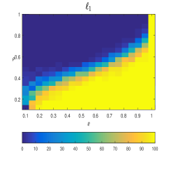
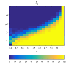
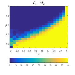
Figure 3: Success percentage of the $\ell_{1}$-, $\ell_{p}$- ($p=0.5)$ and $\ell_{1}-\alpha\ell_{2}$-analysis for recover sparse signals versus the ratios $\varrho$ and $\rho$.

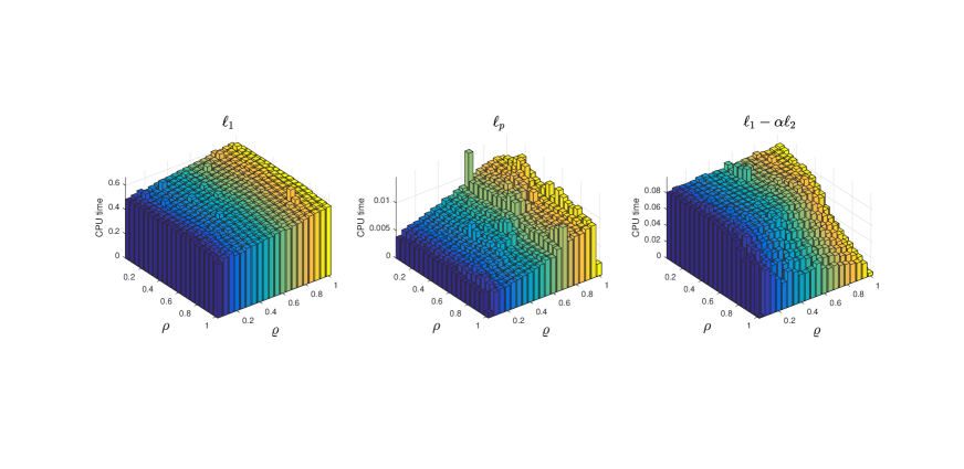
Figure 4: CPU time of the $\ell_{1}$-, $\ell_{p}$- ($p=0.5)$ and $\ell_{1}-\alpha\ell_{2}$-analysis for the sparse signal recovery versus the ratios $\varrho$ and $\rho$.

5.2 Reconstruction of Compressed Sensing Magnetic Resonance Imaging under Tight Frame

In this subsection, we consider the shift-invariant discrete wavelet transform (SIDWT) for tight frame $\bm{D}$, which is a typical tight frame in simulation [1, 2, 11, 24]. And SIDWT is also called as undecimated, translation-invariant, or fully redundant wavelets. In all the experiments, we utilize Daubechies wavelets with 4 decomposition levels in SIDWT.

In CS-MRI, the sampling operator is

$$\bm{A}=\bm{U}\mathcal{F},$$

where $\mathcal{F}$ is the discrete Fourier transform, and $\bm{U}$ is the sampling mask in the frequency space. The matrix $\bm{U}$ is also called the undersampling matrix. We keep samples along certain radial lines passing through the center of the Fourier data ($k$-space). We reconstruct magnetic resonance images (MRI) from incomplete spectral Fourier data: $256\times 256$ Brain MRI and $512\times 512$ Foot MRI (see [29, Section 4.1]) via the $\ell_{1}-\alpha\ell_{2}$-ASSO (1.5).

Similarly, we compare the $\ell_{1}-\alpha\ell_{2}$-ASSO (1.5) to the $\ell_{1}$-analysis and $\ell_{p}$($0<p<1$)-analysis minimization methods. We adopt the pFISTA for tight frames in [35] to solve the $\ell_{1}$-analysis minimization problem. The $\ell_{p}$($0<p<1$)-analysis model is

$$\min_{{\bm{x}}}~{}\lambda\|{\bm{D}}^{\top}{\bm{x}}\|_{p}^{p}+\frac{1}{2}\|\bm{UF}{\bm{x}}-{\bm{b}}\|_{2}^{2},$$ (5.4)

which is solved by the idea of the pFISTA for tight frames. In fact, as shown in section 4, the equality (4.12) is replaced by

$$\bm{x}^{k+1}=\bm{D}~{}\text{Prox}_{\lambda\gamma\ell_{p}}\left(\bm{D}^{\top}\left(\bm{y}^{k}-\gamma\bm{A}^{*}(\bm{A}\bm{y}^{k}-\bm{b})\right)\right),$$ (5.5)

where $0<p<1$ and the notation ${Prox}_{\lambda\ell_{p}}(\bf{b})$ is the proximal operator of $\ell_{p}$ norm, see [41].

The quantitative comparison is done in terms of the relative error (RE) defined as

$$\text{RE}=\frac{\|\hat{\bm{x}}-\bm{x}_{0}\|_{2}}{\|\bm{x}_{0}\|_{2}},$$

where $\bm{x}_{0}$ is the truth image and $\hat{\bm{x}}$ is the reconstructed image. To demonstrate how $\ell_{1}-\alpha\ell_{2}$-ASSO method compares with other methods in terms of image quality, we show the restored versions of Brain images and Foot images and reconstruction errors in Figures 5, 6 and Table 1, respectively.

In Figures 5 and 6, we show the reconstructed images of different methods for $76$ radial sampling lines (sampling rate 30.81$\%$ and 16.17$\%$ for Brain-MRI and Foot-MRI, respectively). By inspecting the recovered images of brain, it can be seen that $\ell_{1}-\alpha\ell_{2}$ method can obtain better performance than other methods. We also record the CPU time of all methods in Table 1.

6 Conclusions

In this paper, we consider the signal and compressed sensing magnetic resonance imaging reconstruction under tight frame. We propose the unconstrained $\ell_{1}-\alpha\ell_{2}$-analysis model (1.5) and (1.8). Based on the restricted isometry property and restricted orthogonality constant adapted to tight frame $\bm{D}$ ($\bm{D}$-RIP and $\bm{D}$-ROC), we develop new vital auxiliary tools (see Propositions 1 and 2) and sufficient conditions of stable recovery (see Theorems 1 and 2). Based on the Projected FISTA [35], we establish the fast and efficient algorithm to solve the unconstrained $\ell_{1}-\alpha\ell_{2}$-analysis model in Section 4. The proposed method has better performance than the $\ell_{p}$-analysis model with $0<p\leq 1$ in numerical examples for the signal and compresses sensing MRI recovery.

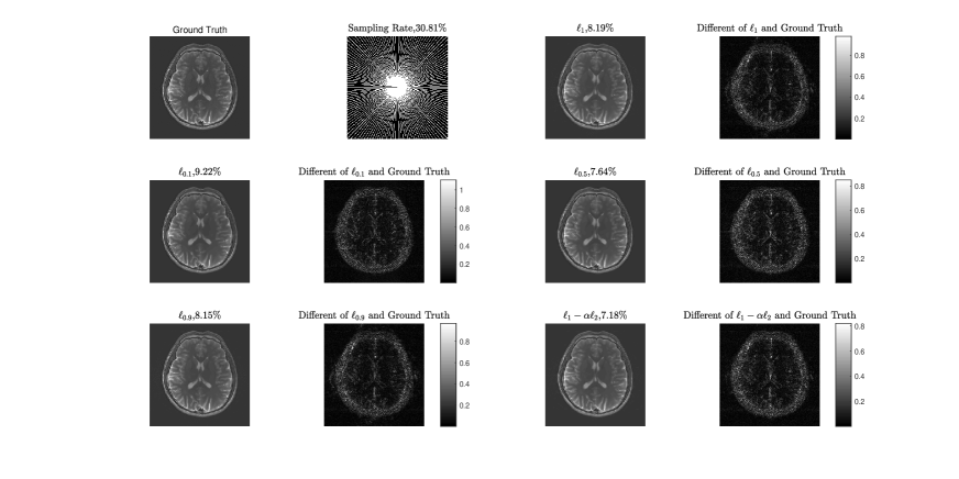
Figure 5: Reconstructed Brain-MRI by the $\ell_{1}$-, $\ell_{p}$- ($0<p<1$) and $\ell_{1}-\alpha\ell_{2}$-analysis. From left to right in the first line: Ground truth, sample lines, $\ell_{1}$ reconstruction image, difference images of $\ell_{1}$ to the ground truth image. From left to right in the second line: $\ell_{0.1}$ reconstruction image, difference images of $\ell_{0.1}$ to the ground truth image, $\ell_{0.5}$ reconstruction image, difference images of $\ell_{0.5}$ to the ground truth image. From left to right in the third line: $\ell_{0.9}$ reconstruction image, difference images of $\ell_{0.9}$ to the ground truth image, $\ell_{1}-\alpha\ell_{2}$ reconstruction image, difference images of $\ell_{1}-\alpha\ell_{2}$ to the ground truth image.

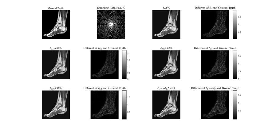
Figure 6: Reconstructed Foot-MRI by the $\ell_{1}$-, $\ell_{p}$- ($0<p<1$) and $\ell_{1}-\alpha\ell_{2}$-analysis. From left to right in the first line: Ground truth, sample lines, $\ell_{1}$ reconstruction image, difference images of $\ell_{1}$ to the ground truth image. From left to right in the second line: $\ell_{0.1}$ reconstruction image, difference images of $\ell_{0.1}$ to the ground truth image, $\ell_{0.5}$ reconstruction image, difference images of $\ell_{0.5}$ to the ground truth image. From left to right in the third line: $\ell_{0.9}$ reconstruction image, difference images of $\ell_{0.9}$ to the ground truth image, $\ell_{1}-\alpha\ell_{2}$ reconstruction image, difference images of $\ell_{1}-\alpha\ell_{2}$ to the ground truth image.

Table 1: The CPU Time (s) of Different reconstruction Models

Image	Sampling Rate	$\ell_{1}$	$\ell_{0.1}$	$\ell_{0.5}$	$\ell_{0.9}$	$\ell_{1}-\alpha\ell_{2}$
Brain-MRI	30.08$\%$	80.9519	164.4825	238.4073	322.2761	85.1567
Foot-MRI	16.17$\%$	308.3546	441.8828	657.7717	857.9363	340.5498

Appendix A The proof of Lemma 3

Proof.

$(\bm{i})$ From the condition (3.1), it follows that

$$\|\bm{D}_{S^{c}}^{\top}\bm{h}\|_{1}-\|\bm{D}_{S^{c}}^{\top}\bm{h}\|_{2} \overset{(a)}{\leq}\|\bm{D}_{S^{c}}^{\top}\bm{h}\|_{1}-\alpha\|\bm{D}_{S^{c}}^{\top}\bm{h}\|_{2}$$

$$\leq a\|\bm{D}_{S}^{\top}\bm{h}\|_{1}+b\|\bm{D}_{S}^{\top}\bm{h}\|_{2}+c\|\bm{D}_{T^{c}}^{\top}\bm{x}\|_{1}+\eta\|{\bm{A}h}\|_{2}+\gamma$$

$$\overset{(b)}{\leq}(a\sqrt{s}+b)\|\bm{D}_{S}^{\top}\bm{h}\|_{2}+c\|\bm{D}_{T^{c}}^{\top}\bm{x}\|_{1}+\eta\|{\bm{A}h}\|_{2}+\gamma$$

$$\leq(s-\sqrt{s})\bigg{(}\frac{a\sqrt{s}+b}{\sqrt{s}-1}\frac{\|\bm{D}_{S}^{\top}\bm{h}\|_{2}}{\sqrt{s}}+\frac{c\|\bm{D}_{T^{c}}^{\top}\bm{x}\|_{1}+\eta\|{\bm{A}h}\|_{2}+\gamma}{s-\sqrt{s}}\bigg{)}$$

$$=:(s-\sqrt{s})\varrho,$$ (A.1)

where $(a)$ is due to $0<\alpha\leq 1$, and $(b)$ follows from the fact $\|\bm{D}_{S}^{\top}\bm{h}\|_{1}\leq\sqrt{s}\|\bm{D}_{S}^{\top}\bm{h}\|_{2}$.

Furthermore, using the fact that $(a-1)\sqrt{s}+(b+1)\geq 0$, i.e., $\frac{a\sqrt{s}+b}{\sqrt{s}-1}\geq 1$, one has

$$\|\bm{D}_{S^{c}}^{\top}\bm{h}\|_{\infty}\leq\frac{\|\bm{D}_{S}^{\top}\bm{h}\|_{1}}{s}\leq\frac{\|\bm{D}_{S}^{\top}\bm{h}\|_{2}}{\sqrt{s}}\leq\frac{\sqrt{s}+\alpha}{\sqrt{s}-1}\frac{\|\bm{D}_{S}^{\top}\bm{h}\|_{2}}{\sqrt{s}}\leq\varrho,$$ (A.2)

where the last inequality is due to the definition of $\varrho$ in (A). By Proposition 2 with $\bm{u}=\|\bm{D}_{S}^{\top}\bm{h}\|_{1}$ and $\bm{v}=\|\bm{D}_{S^{c}}^{\top}\bm{h}\|_{1}$, the desired inequality ((i)) is clear.

$(\bm{ii})$ From the definition of $\tilde{S}$ in (3.3) and $\varrho$ in (A), it follows that

$$\|\bm{D}_{{\tilde{S}}^{c}}^{\top}\bm{h}\|_{\infty}\leq\frac{\varrho}{t-1},$$ (A.3)

and

$$\|\bm{D}_{{\tilde{S}}^{c}}^{\top}\bm{h}\|_{1}-\|\bm{D}_{{\tilde{S}}^{c}}^{\top}\bm{h}\|_{2}= \|\bm{D}_{S^{c}}^{\top}\bm{h}-\bm{D}_{\tilde{S}\setminus S}^{\top}\bm{h}\|_{1}-\|\bm{D}_{S^{c}}^{\top}\bm{h}-\bm{D}_{\tilde{S}\setminus S}^{\top}\bm{h}\|_{2}$$

$$\overset{(a)}{=} \|\bm{D}_{S^{c}}^{\top}\bm{h}\|_{1}-\|\bm{D}_{\tilde{S}\setminus S}^{\top}\bm{h}\|_{1}-\|\bm{D}_{S^{c}}^{\top}\bm{h}-\bm{D}_{\tilde{S}\setminus S}^{\top}\bm{h}\|_{2}$$

$$\overset{(b)}{\leq} \big{(}\|\bm{D}_{S^{c}}^{\top}\bm{h}\|_{1}-\|\bm{D}_{S^{c}}^{\top}\bm{h}\|_{2}\big{)}-(\|\bm{D}_{\tilde{S}\setminus S}^{\top}\bm{h}\|_{1}-\|\bm{D}_{\tilde{S}\setminus S}^{\top}\bm{h}\|_{2})$$

$$\overset{(c)}{\leq} (s-\sqrt{s})\varrho-(\|\bm{D}_{\tilde{S}\setminus S}^{\top}\bm{h}\|_{1}-\|\bm{D}_{\tilde{S}\setminus S}^{\top}\bm{h}\|_{2}),$$ (A.4)

where $(a)$, $(b)$ and $(c)$ follow from $\tilde{S}\setminus S\subseteq S^{c}$, the triangle inequality on $\|\cdot\|_{2}$, and (A), respectively.

For the second term of the above inequality, using Lemma 4 (b) with $S_{1}=\tilde{S}\setminus S$ and $S_{2}=\tilde{S}^{c}$, we derive that

$$\|\bm{D}_{S^{c}}^{\top}\bm{h}\|_{1}-\|\bm{D}_{S^{c}}^{\top}\bm{h}\|_{2}\geq \big{(}\|\bm{D}_{\tilde{S}\setminus S}^{\top}\bm{h}\|_{1}-\|\bm{D}_{\tilde{S}\setminus S}^{\top}\bm{h}\|_{2}\big{)}+\big{(}\|\bm{D}_{\tilde{S}^{c}}^{\top}\bm{h}\|_{1}-\|\bm{D}_{\tilde{S}^{c}}^{\top}\bm{h}\|_{2}\big{)}$$

$$\geq \|\bm{D}_{\tilde{S}\setminus S}^{\top}\bm{h}\|_{1}-\|\bm{D}_{\tilde{S}\setminus S}^{\top}\bm{h}\|_{2}$$

$$\overset{(a)}{\geq} (|\tilde{S}\setminus S|-\sqrt{|\tilde{S}\setminus S|})\min_{i\in\tilde{S}\setminus S}|(\bm{D}_{\tilde{S}\setminus S}^{\top}\bm{h})(i)|$$

$$\overset{(b)}{\geq} (|\tilde{S}\setminus S|-\sqrt{|\tilde{S}\setminus S|})\frac{\varrho}{t-1},$$ (A.5)

where we use Lemma 4 (a) and the definition of $\tilde{S}$ in $(a)$ and $(b)$, respectively. Substituting (A) into (A), there is

$$\|\bm{D}_{\tilde{S}^{c}}^{\top}\bm{h}\|_{1}-\|\bm{D}_{\tilde{S}^{c}}^{\top}\bm{h}\|_{2}\leq\Big{(}(s(t-1)-|\tilde{S}\setminus S|)-(\sqrt{s}(t-1)-\sqrt{|\tilde{S}\setminus S|})\Big{)}\frac{\varrho}{t-1}.$$ (A.6)

Since $t\geq 3$ and $s\geq 2$, as shown in the items (a) and (b) of [18, Page 18], we have

$$|\tilde{S}\setminus S|<s(t-1),\ \ \ \ \sqrt{s(t-1)-|\tilde{S}\setminus S|}\leq\sqrt{s}(t-1)-\sqrt{|\tilde{S}\setminus S|}.$$

Then,

$$\|\bm{D}_{\tilde{S}^{c}}^{\top}\bm{h}\|_{1}-\|\bm{D}_{\tilde{S}^{c}}^{\top}\bm{h}\|_{2}\leq\Big{(}s(t-1)-|\tilde{S}\setminus S|-\sqrt{s(t-1)-|\tilde{S}\setminus S|}\Big{)}\frac{\varrho}{t-1}.$$ (A.7)

Therefore, from (A.3), (A.7) and Proposition 2 with $\bm{u}=\bm{D}_{\tilde{S}}^{\top}{\bm{h}}$, $\bm{v}=\bm{D}_{\tilde{S}^{c}}^{\top}\bm{h}$, it follows that

$$|\langle\bm{AD}\bm{D}_{\tilde{S}}^{\top}{\bm{h}},\bm{AD}\bm{D}_{\tilde{S}^{c}}^{\top}{\bm{h}}\rangle+\langle\bar{\bm{D}}\bm{D}_{\tilde{S}}^{\top}{\bm{h}},\bar{\bm{D}}\bm{D}_{\tilde{S}^{c}}^{\top}{\bm{h}}\rangle|$$

$$\leq\bigg{(}1+\frac{\sqrt{2}}{2}\bigg{)}\theta_{ts,(t-1)s-|\tilde{S}\setminus S|}\sqrt{\lceil(t-1)s\rceil-|\tilde{S}\setminus S|}\frac{\varrho}{t-1}\|\bm{D}_{\tilde{S}}^{\top}{\bm{h}}\|_{2}$$

$$\leq\bigg{(}1+\frac{\sqrt{2}}{2}\bigg{)}\theta_{ts,(t-1)s}\sqrt{\lceil(t-1)s\rceil}\frac{\varrho}{t-1}\|\bm{D}_{\tilde{S}}^{\top}{\bm{h}}\|_{2}.$$ (A.8)

Based on the fact $\bar{\bm{D}}\bm{D}^{\top}=\bm{0}$, the above inequality reduces to the desired ((ii)).

$(\bm{iii})$ For the term $\langle\bm{Ah},\bm{AD}\bm{D}_{\tilde{S}}^{\top}\bm{h}\rangle$, there is

$$|\langle\bm{Ah},\bm{AD}\bm{D}_{\tilde{S}}^{\top}\bm{h}\rangle\big{|}\leq\|\bm{Ah}\|_{2}\|\bm{AD}\bm{D}_{\tilde{S}}^{\top}\bm{h}\|_{2}\overset{(a)}{\leq}\sqrt{1+\delta_{ts}}\|\bm{D}\bm{D}_{\tilde{S}}^{\top}\bm{h}\|_{2}\|\bm{Ah}\|_{2}$$

$$\leq\sqrt{1+\delta_{ts}}\|\bm{D}\|_{2\rightarrow 2}^{1/2}\|\bm{D}_{\tilde{S}}^{\top}\bm{h}\|_{2}\|\bm{Ah}\|_{2}\overset{(b)}{=}\sqrt{1+\delta_{ts}}\|\bm{D}_{\tilde{S}}^{\top}\bm{h}\|_{2}\|\bm{Ah}\|_{2},$$ (A.9)

where $(a)$ is because of the matrix $\bm{A}$ satisfying the $\bm{D}$-RIP of $ts$ order, and $(b)$ follows from $\|\bm{D}\|_{2\rightarrow 2}=\|\bm{D}\bm{D}^{\top}\|_{2\rightarrow 2}^{1/2}=1$.

Next, we will establish the lower bound of $\big{|}\langle\bm{Ah},\bm{AD}\bm{D}_{\tilde{S}}^{\top}\bm{h}\rangle\big{|}$. Note that

$$\big{|}\langle\bm{Ah},\bm{AD}\bm{D}_{\tilde{S}}^{\top}\bm{h}\rangle\big{|}\geq\|\bm{AD}\bm{D}_{\tilde{S}}^{\top}\bm{h}\|_{2}^{2}-\big{|}\langle\bm{AD}\bm{D}_{\tilde{S}^{c}}^{\top}\bm{h},\bm{AD}\bm{D}_{\tilde{S}}^{\top}\bm{h}\rangle\big{|}.$$

From Proposition 1 with $\bm{v}=\bm{D}_{\tilde{S}^{c}}^{\top}\bm{h}$ and $\bar{\bm{D}}\bm{D}^{\top}=\bm{0}$, it follows that

$$\|\bm{AD}\bm{D}_{\tilde{S}}^{\top}\bm{h}\|_{2}^{2}=\|\bm{AD}\bm{D}_{\tilde{S}}^{\top}\bm{h}\|_{2}^{2}+\|\bar{\bm{D}}\bm{D}_{\tilde{S}}^{\top}\bm{h}\|_{2}^{2}\geq(1-\delta_{ts})\|\bm{D}_{\tilde{S}}^{\top}\bm{h}\|_{2}^{2}.$$

By ((ii)) in item (ii) and $\varrho$ in (A), we have

$$\big{|}\langle\bm{AD}\bm{D}_{\tilde{S}^{c}}^{\top}\bm{h},\bm{AD}\bm{D}_{\tilde{S}}^{\top}\bm{h}\rangle\big{|}\leq\theta_{ts,(t-1)s}\sqrt{\lceil(t-1)s\rceil}\bigg{(}1+\frac{\sqrt{2}}{2}\bigg{)}\frac{\varrho}{t-1}\|\bm{D}_{\tilde{S}}^{\top}\bm{h}\|_{2}$$

Then,

$$\big{|}\langle\bm{Ah},\bm{AD}\bm{D}_{\tilde{S}}^{\top}\bm{h}\rangle\big{|}$$

$$\geq(1-\delta_{ts})\|\bm{D}_{\tilde{S}}^{\top}\bm{h}\|_{2}^{2}-\theta_{ts,(t-1)s}\bigg{(}1+\frac{\sqrt{2}}{2}\bigg{)}\frac{\sqrt{\lceil(t-1)s\rceil}}{t-1}\|\bm{D}_{\tilde{S}}^{\top}\bm{h}\|_{2}$$

$$\cdot\bigg{(}\frac{a\sqrt{s}+b}{\sqrt{s}-1}\frac{\|\bm{D}_{S}^{\top}\bm{h}\|_{2}}{\sqrt{s}}+\frac{c\|\bm{D}_{T^{c}}^{\top}\bm{x}\|_{1}+\eta\|{\bm{A}h}\|_{2}+\gamma}{s-\sqrt{s}}\bigg{)}$$

$$\geq\bigg{(}1-\delta_{ts}-\bigg{(}1+\frac{\sqrt{2}}{2}\bigg{)}\sqrt{\frac{\lceil(t-1)s\rceil}{(t-1)^{2}s}}\frac{a\sqrt{s}+b}{\sqrt{s}-1}\theta_{ts,(t-1)s}\bigg{)}\|\bm{D}_{\tilde{S}}^{\top}\bm{h}\|_{2}^{2}$$

$$-\theta_{ts,(t-1)s}\bigg{(}1+\frac{\sqrt{2}}{2}\bigg{)}\frac{\sqrt{\lceil(t-1)s\rceil}}{t-1}\frac{c\|\bm{D}_{T^{c}}^{\top}\bm{x}\|_{1}+\eta\|{\bm{A}h}\|_{2}+\gamma}{s-\sqrt{s}}\|\bm{D}_{\tilde{S}}^{\top}\bm{h}\|_{2},$$ (A.10)

where the last inequality is due to $S\subseteq\tilde{S}$. Combining (A) with (A), one has

$$\bigg{(}1-\delta_{ts}-\sqrt{\frac{\lceil(t-1)s\rceil}{(t-1)^{2}s}}\frac{(\sqrt{2}+1)(\sqrt{s}+\alpha)}{\sqrt{2}(\sqrt{s}-1)}\theta_{ts,(t-1)s}\bigg{)}\|\bm{D}_{\tilde{S}}^{\top}\bm{h}\|_{2}^{2}$$

$$-\bigg{(}\theta_{ts,(t-1)s}\frac{\sqrt{2}+1}{\sqrt{2}}\frac{\sqrt{\lceil(t-1)s\rceil}}{t-1}\frac{c\|\bm{D}_{T^{c}}^{\top}\bm{x}\|_{1}+\eta\|\bm{Ah}\|_{2}+\gamma}{s-\sqrt{s}}$$

$$+\sqrt{1+\delta_{ts}}\|\bm{Ah}\|_{2}\bigg{)}\|\bm{D}_{\tilde{S}}^{\top}\bm{h}\|_{2}\leq 0.$$

Therefore, using (3.5) we derive that

$$\|\bm{D}_{S}^{\top}\bm{h}\|_{2}\leq\|\bm{D}_{\tilde{S}}^{\top}\bm{h}\|_{2}$$

$$\leq\frac{\theta_{ts,(t-1)s}}{(1-\rho_{s,t})}\frac{\sqrt{2}+1}{\sqrt{2}}\frac{\sqrt{\lceil(t-1)s\rceil}}{(t-1)(s-\sqrt{s})}\left(c\|\bm{D}_{T^{c}}^{\top}\bm{x}\|_{1}+\gamma\right)$$

$$+\bigg{(}\frac{\theta_{ts,(t-1)s}}{(1-\rho_{s,t})}\frac{\sqrt{2}+1}{\sqrt{2}}\frac{\sqrt{\lceil(t-1)s\rceil}}{(t-1)(s-\sqrt{s})}+\frac{\sqrt{1+\delta_{ts}}}{1-\rho_{s,t}}\bigg{)}\eta\|\bm{Ah}\|_{2},$$ (A.11)

where $\eta\geq 1$.

$(\bm{iv})$ As shown in the proof of $(iii)$, we can prove the item (iv) by item (i) and (3.7). We here omit the detail proof.

$(\bm{v})$ The idea of the proof is the argument in [17, Step 2]. By (3.1) and the fact that $\|\bm{D}_{S^{c}}^{\top}\bm{h}\|_{\infty}\leq\|\bm{D}_{S}^{\top}\bm{h}\|_{1}/s\leq\|\bm{D}_{S}^{\top}\bm{h}\|_{2}/\sqrt{s}$, we have

$$\|\bm{D}_{S^{c}}^{\top}\bm{h}\|_{2}^{2}\leq\|\bm{D}_{S^{c}}^{\top}\bm{h}\|_{1}\|\bm{D}_{S^{c}}^{\top}\bm{h}\|_{\infty}$$

$$\leq\big{(}a\|\bm{D}_{S}^{\top}\bm{h}\|_{1}+b\|\bm{D}_{S}^{\top}\bm{h}\|_{2}+c\|\bm{D}_{T^{c}}^{\top}\bm{x}\|_{1}+\eta\|{\bm{Ah}}\|_{2}+\gamma+\alpha\|\bm{D}_{S^{c}}^{\top}\bm{h}\|_{2}\big{)}\frac{\|\bm{D}_{S}^{\top}\bm{h}\|_{2}}{\sqrt{s}}$$

$$\leq\frac{\alpha\|\bm{D}_{S}^{\top}\bm{h}\|_{2}}{\sqrt{s}}\|\bm{D}_{S^{c}}^{\top}\bm{h}\|_{2}+\frac{a\sqrt{s}+b}{\sqrt{s}}\|\bm{D}_{S}^{\top}\bm{h}\|_{2}^{2}+\frac{c\|\bm{D}_{T^{c}}^{\top}\bm{x}\|_{1}+\eta\|{\bm{Ah}}\|_{2}+\gamma}{\sqrt{s}}\|\bm{D}_{S}^{\top}\bm{h}\|_{2}.$$

That is,

$$\bigg{(}\|\bm{D}_{S^{c}}^{\top}\bm{h}\|_{2}-\frac{\alpha\|\bm{D}_{S}^{\top}\bm{h}\|_{2}}{2\sqrt{s}}\bigg{)}^{2}$$

$$\leq\bigg{(}\frac{\alpha^{2}}{4s}+\frac{a\sqrt{s}+b}{\sqrt{s}}\bigg{)}\|\bm{D}_{S}^{\top}\bm{h}\|_{2}^{2}+\frac{c\|\bm{D}_{T^{c}}^{\top}\bm{x}\|_{1}+\eta\|{\bm{Ah}}\|_{2}+\gamma}{\sqrt{s}}\|\bm{D}_{S}^{\top}\bm{h}\|_{2}.$$

Then, we obtain

$$\|\bm{D}_{S^{c}}^{\top}\bm{h}\|_{2}$$

$$\leq\Bigg{(}\sqrt{\frac{a\sqrt{s}+b}{\sqrt{s}}+\frac{\alpha^{2}}{4s}}+\frac{\alpha}{2\sqrt{s}}\Bigg{)}\|\bm{D}_{S}^{\top}\bm{h}\|_{2}+\sqrt{\frac{c\|\bm{D}_{T^{c}}^{\top}\bm{x}\|_{1}+\eta\|{\bm{Ah}}\|_{2}+\gamma}{\sqrt{s}}\|\bm{D}_{S}^{\top}\bm{h}\|_{2}}$$

$$\leq\Bigg{(}\sqrt{\frac{a\sqrt{s}+b}{\sqrt{s}}+\frac{\alpha^{2}}{4s}}+\frac{\alpha+\bar{\varepsilon}}{2\sqrt{s}}\Bigg{)}\|\bm{D}_{S}^{\top}\bm{h}\|_{2}+\frac{1}{2\bar{\varepsilon}}\big{(}c\|\bm{D}_{T^{c}}^{\top}\bm{x}\|_{1}+\eta\|\bm{Ah}\|_{2}+\gamma\big{)},$$ (A.12)

where the second inequality comes from the basic inequality $\sqrt{|a||b|}\leq\frac{|a|+|b|}{2}$, and the constant $\bar{\varepsilon}>0$. ∎

References

- [1] Christopher A Baker, Kevin King, Dong Liang, and Leslie Ying. Translational-invariant dictionaries for compressed sensing in magnetic resonance imaging. In 2011 IEEE International Symposium on Biomedical Imaging: From Nano to Macro, pages 1602–1605. IEEE, 2011.
- [2] Richard Baraniuk et al. Rice wavelet toolbox, 2009.
- [3] Amir Beck and Marc Teboulle. A fast iterative shrinkage-thresholding algorithm for linear inverse problems. SIAM journal on imaging sciences, 2(1):183–202, 2009.
- [4] Alfred M Bruckstein, David L Donoho, and Michael Elad. From sparse solutions of systems of equations to sparse modeling of signals and images. SIAM review, 51(1):34–81, 2009.
- [5] Jian-Feng Cai, Hui Ji, Zuowei Shen, and Gui-Bo Ye. Data-driven tight frame construction and image denoising. Applied and Computational Harmonic Analysis, 37(1):89–105, 2014.
- [6] T Tony Cai and Anru Zhang. Compressed sensing and affine rank minimization under restricted isometry. IEEE Transactions on Signal Processing, 61(13):3279–3290, 2013.
- [7] Emmanuel J Candès, Yonina C Eldar, Deanna Needell, and Paige Randall. Compressed sensing with coherent and redundant dictionaries. Applied and Computational Harmonic Analysis, 31(1):59–73, 2011.
- [8] Emmanuel J Candès, Justin K Romberg, and Terence Tao. Stable signal recovery from incomplete and inaccurate measurements. Communications on Pure and Applied Mathematics: A Journal Issued by the Courant Institute of Mathematical Sciences, 59(8):1207–1223, 2006.
- [9] Emmanuel J Candès and Terence Tao. Decoding by linear programming. IEEE transactions on information theory, 51(12):4203–4215, 2005.
- [10] Rick Chartrand and Valentina Staneva. Restricted isometry properties and nonconvex compressive sensing. Inverse Problems, 24(3):035020, 2008.
- [11] Ronald R Coifman and David L Donoho. Translation-invariant de-noising. In Wavelets and statistics, pages 125–150. Springer, 1995.
- [12] Ingrid Daubechies, Michel Defrise, and Christine De Mol. An iterative thresholding algorithm for linear inverse problems with a sparsity constraint. Communications on Pure and Applied Mathematics: A Journal Issued by the Courant Institute of Mathematical Sciences, 57(11):1413–1457, 2004.
- [13] Ingrid Daubechies, Ronald DeVore, Massimo Fornasier, and C Sinan Güntürk. Iteratively reweighted least squares minimization for sparse recovery. Communications on Pure and Applied Mathematics: A Journal Issued by the Courant Institute of Mathematical Sciences, 63(1):1–38, 2010.
- [14] David L Donoho. Compressed sensing. IEEE Transactions on information theory, 52(4):1289–1306, 2006.
- [15] David L Donoho, Michael Elad, and Vladimir N Temlyakov. Stable recovery of sparse overcomplete representations in the presence of noise. IEEE Transactions on Information Theory, 52(1):6–18, 2005.
- [16] Michael Elad, Peyman Milanfar, and Ron Rubinstein. Analysis versus synthesis in signal priors. Inverse problems, 23(3):947, 2007.
- [17] Huanmin Ge, Wengu Chen, and Michael K Ng. New restricted isometry property analysis for minimization methods. SIAM Journal on Imaging Sciences, Accepted, 2021.
- [18] Huanmin Ge and Peng Li. The dantzig selector: recovery of signal via minimization. Inverse Problems, 38(1):015006, 2021.
- [19] Pengbo Geng and Wengu Chen. Unconstrained minimization for sparse recovery via mutual coherence. Mathematical Foundations of Computing, 3(2):65–79, 2020.
- [20] Martin Genzel, Gitta Kutyniok, and Maximilian März. -analysis minimization and generalized (co-) sparsity: When does recovery succeed? Applied and Computational Harmonic Analysis, 52:82–140, 2021.
- [21] Matthieu Guerquin-Kern, M Haberlin, Klaas Paul Pruessmann, and Michael Unser. A fast wavelet-based reconstruction method for magnetic resonance imaging. IEEE transactions on medical imaging, 30(9):1649–1660, 2011.
- [22] Deguang Han, Keri Kornelson, Eric Weber, and David Larson. Frames for undergraduates, volume 40. American Mathematical Soc., 2007.
- [23] Yue Huang, John Paisley, Qin Lin, Xinghao Ding, Xueyang Fu, and Xiao-Ping Zhang. Bayesian nonparametric dictionary learning for compressed sensing mri. IEEE Transactions on Image Processing, 23(12):5007–5019, 2014.
- [24] Mohammad H Kayvanrad, A Jonathan McLeod, John SH Baxter, Charles A McKenzie, and Terry M Peters. Stationary wavelet transform for under-sampled mri reconstruction. Magnetic resonance imaging, 32(10):1353–1364, 2014.
- [25] Ming-Jun Lai, Yangyang Xu, and Wotao Yin. Improved iteratively reweighted least squares for unconstrained smoothed minimization. SIAM Journal on Numerical Analysis, 51(2):927–957, 2013.
- [26] Zongying Lai, Xiaobo Qu, Yunsong Liu, Di Guo, Jing Ye, Zhifang Zhan, and Zhong Chen. Image reconstruction of compressed sensing mri using graph-based redundant wavelet transform. Medical image analysis, 27:93–104, 2016.
- [27] Peng Li and Wengu Chen. Signal recovery under cumulative coherence. Journal of Computational and Applied Mathematics, 346:399–417, 2019.
- [28] Peng Li, Wengu Chen, Huanmin Ge, and Michael K. Ng. minimization methods for signal and image reconstruction with impulsive noise removal. Inverse Problems, 36(5):055009, 2020.
- [29] Peng Li, Wengu Chen, and Michael K Ng. Compressive total variation for image reconstruction and restoration. Computers & Mathematics with Applications, 80(5):874–893, 2020.
- [30] Song Li and Junhong Lin. Compressed sensing with coherent tight frames via -minimization for . Inverse Problems & Imaging, 8(3):761, 2014.
- [31] Junhong Lin and Song Li. Restricted -isometry properties adapted to frames for nonconvex -analysis. IEEE Transactions on Information Theory, 62(8):4733–4747, 2016.
- [32] Junhong Lin, Song Li, and Yi Shen. New bounds for restricted isometry constants with coherent tight frames. IEEE Transactions on Signal Processing, 61(3):611–621, 2013.
- [33] Tianxiang Liu and Ting Kei Pong. Further properties of the forward–backward envelope with applications to difference-of-convex programming. Computational Optimization and Applications, 67(3):489–520, 2017.
- [34] Yunsong Liu, Jian-Feng Cai, Zhifang Zhan, Di Guo, Jing Ye, Zhong Chen, and Xiaobo Qu. Balanced sparse model for tight frames in compressed sensing magnetic resonance imaging. PloS one, 10(4):e0119584, 2015.
- [35] Yunsong Liu, Zhifang Zhan, Jian-Feng Cai, Di Guo, Zhong Chen, and Xiaobo Qu. Projected iterative soft-thresholding algorithm for tight frames in compressed sensing magnetic resonance imaging. IEEE transactions on medical imaging, 35(9):2130–2140, 2016.
- [36] Yifei Lou and Ming Yan. Fast minimization via a proximal operator. Journal of Scientific Computing, 74(2):767–785, 2018.
- [37] Yifei Lou, Penghang Yin, Qi He, and Jack Xin. Computing sparse representation in a highly coherent dictionary based on difference of and . Journal of Scientific Computing, 64(1):178–196, 2015.
- [38] Michael Lustig, David Donoho, and John M Pauly. Sparse mri: The application of compressed sensing for rapid mr imaging. Magnetic Resonance in Medicine: An Official Journal of the International Society for Magnetic Resonance in Medicine, 58(6):1182–1195, 2007.
- [39] Michael Lustig, David L Donoho, Juan M Santos, and John M Pauly. Compressed sensing mri. IEEE signal processing magazine, 25(2):72–82, 2008.
- [40] Angshul Majumdar and Rabab K Ward. Energy efficient eeg sensing and transmission for wireless body area networks: A blind compressed sensing approach. Biomedical Signal Processing and Control, 20:1–9, 2015.
- [41] Goran Marjanovic and Victor Solo. On optimization and matrix completion. IEEE Transactions on signal processing, 60(11):5714–5724, 2012.
- [42] Nicolai Meinshausen and Peter Bühlmann. High-dimensional graphs and variable selection with the lasso. Annals of Statistics, 34(3), 2006.
- [43] Sangnam Nam, Mike E Davies, Michael Elad, and Rémi Gribonval. The cosparse analysis model and algorithms. Applied and Computational Harmonic Analysis, 34(1):30–56, 2013.
- [44] Xiaobo Qu, Yingkun Hou, Fan Lam, Di Guo, Jianhui Zhong, and Zhong Chen. Magnetic resonance image reconstruction from undersampled measurements using a patch-based nonlocal operator. Medical image analysis, 18(6):843–856, 2014.
- [45] Saiprasad Ravishankar and Yoram Bresler. Mr image reconstruction from highly undersampled -space data by dictionary learning. IEEE transactions on medical imaging, 30(5):1028–1041, 2011.
- [46] Mrinmoy Sandilya and SR Nirmala. Compressed sensing trends in magnetic resonance imaging. Engineering science and technology, an international journal, 20(4):1342–1352, 2017.
- [47] Zhao Tan, Yonina C Eldar, Amir Beck, and Arye Nehorai. Smoothing and decomposition for analysis sparse recovery. IEEE Transactions on Signal Processing, 62(7):1762–1774, 2014.
- [48] S. S. Vasanawala, M. J. Murphy, Marcus T. Alley, P. Lai, Kurt Keutzer, John M. Pauly, and Michael Lustig. Practical parallel imaging compressed sensing mri: Summary of two years of experience in accelerating body mri of pediatric patients. In 2011 ieee international symposium on biomedical imaging: From nano to macro, pages 1039–1043. IEEE, 2011.
- [49] Martin Vetterli, Jelena Kovacevic, and Vivek K Goyal. Foundations of signal processing tables. 2012.
- [50] Wendong Wang and Jianjun Wang. Improved sufficient condition of -minimisation for robust signal recovery. Electronics Letters, 55(22):1199–1201, 2019.
- [51] Jong Chul Ye. Compressed sensing mri: a review from signal processing perspective. BMC Biomedical Engineering, 1(1):1–17, 2019.
- [52] Penghang Yin, Yifei Lou, Qi He, and Jack Xin. Minimization of for compressed sensing. SIAM Journal on Scientific Computing, 37(1):A536–A563, 2015.
- [53] Zhifang Zhan, Jian-Feng Cai, Di Guo, Yunsong Liu, Zhong Chen, and Xiaobo Qu. Fast multiclass dictionaries learning with geometrical directions in mri reconstruction. IEEE Transactions on biomedical engineering, 63(9):1850–1861, 2015.
- [54] Peng Zhao and Bin Yu. On model selection consistency of lasso. Journal of Machine Learning Research, 7(12):2541–2563, 2006.