The Classical Multidimensional Scaling Revisited

Abstract

We reexamine the the classical multidimensional scaling (MDS). We study some special cases, in particular, the exact solution for the sub-space formed by the 3 dimensional principal coordinates is derived. Also we give the extreme case when the points are collinear. Some insight into the effect on the MDS solution of the excluded eigenvalues (could be both positive as well as negative) of the doubly centered matrix is provided. As an illustration, we work through an example to understand the distortion in the MDS construction with positive and negative eigenvalues.

1 Basics of the classical MDS

We recall in this section some basics of the classical MDS from Mardia et al (1979, Section 14.2). Let us denote the $n\times n$ distance matrix as $\mathbf{D}=(d_{ij})$ and form the matrix $\mathbf{A}$

$$\mathbf{A}=\{a_{ij}\},a_{ij} =-\frac{1}{2}d_{ij}^{2},$$ (1)

and define the corresponding doubly centered matrix $\mathbf{B}$,

$$\mathbf{B}=\mathbf{H}\mathbf{A}\mathbf{H},$$ (2)

where $\mathbf{H}=\mathbf{I_{n}}-\frac{\underaccent{\bar}{1}_{n}\underaccent{\bar}{1}_{n}^{T}}{n}$ is the centering matrix in the standard notation. We can rewrite $\mathbf{B}$ as

$$\mathbf{B}=\mathbf{X}\mathbf{X}^{T},$$ (3)

and the $n\times n$ matrix $\mathbf{X}$ of the principal coordinates in the Euclidean space (assuming that $\mathbf{B}$ is semi-positive) is given by

$$\mathbf{X}=\mathbf{\Gamma}\mathbf{\Lambda}^{\frac{1}{2}}=({\lambda_{1}}^{\frac{1}{2}}{\gamma_{1}},{\lambda_{2}}^{\frac{1}{2}}{\gamma_{2}}\ldots,{\lambda_{n}}^{\frac{1}{2}}{\gamma_{n}})=(\underaccent{\bar}{x}_{(1)},\underaccent{\bar}{x}_{(2)},\ldots,\underaccent{\bar}{x}_{(n)}),$$ (4)

where

$$\underaccent{\bar}{x}_{(i)}={\lambda_{i}}^{\frac{1}{2}}{\underaccent{\bar}{\gamma}_{i}},i=1,\ldots,n,$$

with the spectral decomposition of $\mathbf{B}$

$$\mathbf{B}=\mathbf{\Gamma}\mathbf{\Lambda}\mathbf{\Gamma}^{T},$$ (5)

and

$$\mathbf{\Gamma}=\{\gamma_{ij}\}=(\underaccent{\bar}{\gamma}_{1},\ldots,\underaccent{\bar}{\gamma}_{n})$$

is the orthogonal matrix of eigenvectors and $\mathbf{\Lambda}$ is the diagonal matrix of eigenvalues,

$$\mathbf{\Lambda}=\text{Diag}\{\lambda_{1},\ldots,\lambda_{n}\}.$$

Indeed, the $n$ principal coordinates $\underaccent{\bar}{x}_{i},i=1,2,\ldots,n$ are the rows of $\mathbf{X}$, namely,

$$\mathbf{X}=\begin{pmatrix}\underaccent{\bar}{x}^{T}_{1}\\ \underaccent{\bar}{x}^{T}_{2}\\ \vdots\\ \underaccent{\bar}{x}^{T}_{n}\end{pmatrix},\underaccent{\bar}{x}_{i}^{T}=({\lambda_{1}}^{\frac{1}{2}}{\gamma}_{i1},\ldots,{\lambda_{n}}^{\frac{1}{2}}{\gamma}_{in}),i=1,\ldots,n.$$ (6)

We can use any “subpart” of $\mathbf{X}$ to define the principal coordinates of a low dimensional space as our MDS solution. Note that the last eigenvalue $\lambda_{n}$ is zero so at least $\underaccent{\bar}{x}_{(n)}=0$ so we can work on the remaining $n-1$ dimensional coordinates.

Note that, for simplicity, we have taken $\mathbf{X}$ as the $n\times n$ matrix rather than $n\times p$ matrix. We now show that, for any dissimilarity matrix $\mathbf{D}$ with real entries but not necessarily semi-positive definite $\mathbf{B}$ as in above, $\lambda_{1}$ will be always positive. We have

$$tr(\mathbf{B})=tr(\mathbf{H}^{2}\mathbf{A})=tr(\mathbf{H}\mathbf{A})=tr(\mathbf{A})-tr(\underaccent{\bar}{1}^{T}\mathbf{A}\underaccent{\bar}{1})/n$$

so that

$$\sum_{i=1}^{n}\lambda_{i}=\sum_{i<j}d_{i,j}^{2}/n>0.$$ (7)

Hence $\lambda_{1}>0$. Thus implying that we can always ”fit” one-dimensional configuration for any distance/ dissimilarity matrix.

Let us now consider the case when the n points lie on a line then we will have only one non-zero eigenvalue $\lambda$ of $\mathbf{B}$ so from (7), it is given by

$$\lambda=\sum_{i<j}d_{i,j}^{2}/n.$$

• For n=3 with points on the line with the inter-point distances as $a,b,c$, we have $\lambda=(a^{2}+b^{2}+c^{2})/3,$ where if $AB=a,BC=b,AC=c$ with the points $A,B,C$ in that order then $a+b=c.$

• If the points are $1,2,\ldots,n$ then we find that $\lambda=n(n^{2}-1)/12$ so with the distances scaled to (0,1), we have $\lambda$ = $n(n^{2}-1)/12(n-1)^{2}$ and $\lambda$=O(n).

2 The MDS solution for $2\times 2$ distance matrix

Let $X=(\underaccent{\bar}{x}_{(1)},\underaccent{\bar}{x}_{(2)})$ where $\underaccent{\bar}{x}_{k},k=1,2$ are the coordinates in 2 dimensions. Suppose the two points are separated by a distance $d$. We have

$$D=\begin{pmatrix}0&d\\ d&0\end{pmatrix},\hskip 3.0ptB=\begin{pmatrix}\frac{d^{2}}{4}&\frac{-d^{2}}{4}\\ \frac{-d^{2}}{4}&\frac{d^{2}}{4}\end{pmatrix}.$$

The eigenvalues of $$\mathbf{B}$$ are given by

$$|\mathbf{B}-\lambda\mathbf{I}_{2}| =\lambda^{2}-2\lambda\frac{d^{2}}{4}.$$ (8)

Solving (8) gives the eigenvalues

$$\lambda_{1}=\frac{d^{2}}{2}\ \text{and}\ \lambda_{2}=0,$$

with the corresponding eigenvectors

$$\underaccent{\bar}{\gamma}_{1}=\left(\frac{1}{\sqrt{2}},\frac{-1}{\sqrt{2}}\right)^{T}\ \text{and}\ \underaccent{\bar}{\gamma}_{2}=\left(\frac{1}{\sqrt{2}},\frac{1}{\sqrt{2}}\right)^{T}.$$

Now using  $$\underaccent{\bar}{x}_{(k)}=\lambda_{k}^{\frac{1}{2}}\underaccent{\bar}{\gamma}_{k} \mathbf{X}$$ from (4), and we get for

$$\underaccent{\bar}{x}_{(1)}=\left(\frac{d}{2},\frac{-d}{2}\right)^{T}\hskip 3.0pt \text{and}\hskip 3.0pt\underaccent{\bar}{x}_{(2)}=\left(0,0\right)^{T}.$$ (9)

So the principal coordinates from (6) are

$$\underaccent{\bar}{x}_{1}=\left(\frac{d}{2},0\right)^{T}\hskip 3.0pt\text{and}\hskip 3.0pt\underaccent{\bar}{x}_{2}=\left(-\frac{d}{2},0\right)^{T}.$$ (10)

To get a lower dimensional coordinate space (one dimensional), we can simply use, along the line ( $x$- axis), the following two points:

$$x_{1}=\frac{d}{2},\quad x_{2}=-\frac{d}{2}.$$

We can now shift $x$ conveniently by using $x^{*}$ = $x+\frac{d}{2}$ so we have the new coordinates

$$x^{*}_{1}=d,\quad x^{*}_{2}=0$$

along the $x^{*}$- axis in one dimension with the origin at $x^{*}_{2}$.

The solution (10) is trivial as the points only require placing a distance $d$ apart to be recovered, although it does serve as a pointer for the $3\times 3$ distance matrix in the next section.

3 The MDS solution for $3\times 3$ distance matrix

We now extend the last section of the $2\times 2$ distance matrix to the $3\times 3$ distance matrix where in principle, we need to follow the same steps. Let now $\mathbf{X}=(\underaccent{\bar}{x}_{(1)},\underaccent{\bar}{x}_{(2)},\underaccent{\bar}{x}_{(3)})$, where $\underaccent{\bar}{x}_{k},k=1,2,3$ give the coordinates of points in three dimensions . Let

$$\mathbf{D} =\begin{pmatrix}0&a&b\\ a&0&c\\ b&c&0\end{pmatrix}.$$ (11)

Then it can be seen that

$$\mathbf{B} =\frac{1}{18}\begin{pmatrix}4a^{2}+4b^{2}-2c^{2}&-5a^{2}+b^{2}+c^{2}&a^{2}-5b^{2}+c^{2}\\ -5a^{2}+b^{2}+c^{2}&4a^{2}-2b^{2}+4c^{2}&a^{2}+b^{2}-5c^{2}\\ a^{2}-5b^{2}+c^{2}&a^{2}+b^{2}-5c^{2}&-2a^{2}+4b^{2}+4c^{2}\end{pmatrix}.$$

and

$$|\mathbf{B}-\lambda\mathbf{I}_{3}| =\left(\frac{-1}{6}(a^{2}b^{2}+a^{2}c^{2}+b^{2}c^{2})+\frac{1}{12}(a^{4}+b^{4}+c^{4})\right)\lambda$$

$$\quad\quad+\frac{1}{3}(a^{2}+b^{2}+c^{2})\lambda^{2}-\lambda^{3}.$$ (12)

Let

$$\Delta =\sqrt{a^{4}+b^{4}+c^{4}-a^{2}b^{2}-a^{2}c^{2}-b^{2}c^{2}}.$$ (13)

Solving (12) we find that the eigenvalues are

$$\lambda_{1} =\frac{1}{6}(a^{2}+b^{2}+c^{2}+2\Delta),$$

$$\lambda_{2} =\frac{1}{6}(a^{2}+b^{2}+c^{2}-2\Delta),$$

$$\text{and}\ \lambda_{3} =0.$$ (14)

We show below in the proof of Theorem 1 that $$\Delta \mathbf{B} \mathbf{R}$$ is always non-negative. To find the corresponding eigenvectors, is rotated using a Helmert rotation matrix

$$\mathbf{R} =\begin{pmatrix}\frac{1}{\sqrt{3}}&\frac{1}{\sqrt{3}}&\frac{1}{\sqrt{3}}\\ \frac{-1}{\sqrt{2}}&0&\frac{1}{\sqrt{2}}\\ \frac{1}{\sqrt{6}}&\frac{-2}{\sqrt{6}}&\frac{1}{\sqrt{6}}\end{pmatrix}.$$

That is

$$\mathbf{R}\mathbf{B}\mathbf{R}^{T} =\begin{pmatrix}0&0&0\\ 0&\frac{b^{2}}{2}&\frac{(-a^{2}+c^{2})}{2\sqrt{3}}\\ 0&\frac{(-a^{2}+c^{2})}{2\sqrt{3}}&\frac{(2a^{2}-b^{2}+2c^{2})}{6}\end{pmatrix}=\begin{pmatrix}0&0&0\\ 0&\sigma^{2}_{1,1}&\sigma^{2}_{1,2}\\ 0&\sigma^{2}_{1,2}&\sigma^{2}_{2,2}\end{pmatrix}$$ (15)

which has a $2\times 2$ symmetric matrix nested within a $3\times 3$ null matrix. We first give the eigenvectors of $\mathbf{R}^{T}\mathbf{B}\mathbf{R}$ by using a result of Mardia et al (1979, page 246, Exercise 8.1.1) ,

$$\underaccent{\bar}{\phi}_{1} =\begin{pmatrix}0\\ \sigma^{2}_{2,2}-\sigma^{2}_{1,1}+\Theta\\ -2\sigma^{2}_{1,2}\end{pmatrix}\hskip 3.0pt\text{and}\hskip 3.0pt\underaccent{\bar}{\phi}_{2}=\begin{pmatrix}0\\ 2\sigma^{2}_{1,2}\\ \sigma^{2}_{2,2}-\sigma^{2}_{1,1}+\Theta\end{pmatrix}$$ (16)

where $$\Theta=\sqrt{(\sigma^{2}_{1,1}-\sigma^{2}_{2,2})^{2}+4\sigma^{4}_{1,2}} \mathbf{R} \mathbf{B}$$. Next, the rotation is reversed by pre-multiplying the unnormalized eigenvectors (16) by to deduce the eigenvectors of

$$\underaccent{\bar}{\gamma}_{1} =\begin{pmatrix}b^{2}-c^{2}+\Delta\\ -a^{2}+c^{2}\\ a^{2}-b^{2}-\Delta\end{pmatrix},\ \underaccent{\bar}{\gamma}_{2}=\begin{pmatrix}2a^{2}-b^{2}-c^{2}-\Delta\\ -a^{2}+2b^{2}-c^{2}+2\Delta\\ -a^{2}-b^{2}+2c^{2}-\Delta\end{pmatrix},\ \underaccent{\bar}{\gamma}_{3}=\begin{pmatrix}1\\ 1\\ 1\end{pmatrix}$$ (17)

where $$\Delta \underaccent{\bar}{x}_{(k)}=\lambda_{k}^{\frac{1}{2}}\underaccent{\bar}{\gamma}_{k} \mathbf{X}$$ is given by (13). Now using   from (4), and we get for

$$\underaccent{\bar}{x}_{(1)} =w_{1}\begin{pmatrix}b^{2}-c^{2}+\Delta\\ -a^{2}+c^{2}\\ a^{2}-b^{2}-\Delta\end{pmatrix}\text{where}$$

$$w_{1} =\sqrt{(a^{2}+b^{2}+c^{2}+2\Delta)/(12\delta)},$$ (18)

$$\delta =\Delta(2\Delta-a^{2}+2b^{2}-c^{2})$$

and

$$\underaccent{\bar}{x}_{(2)} =w_{2}\begin{pmatrix}2a^{2}-b^{2}-c^{2}-\Delta\\ -a^{2}+2b^{2}-c^{2}+2\Delta\\ -a^{2}-b^{2}+2c^{2}-\Delta\end{pmatrix}\text{where}$$

$$w_{2} =\sqrt{(a^{2}+b^{2}+c^{2}-2\Delta)/(12\delta)},$$ (19)

$$\delta =\Delta(2\Delta-a^{2}+2b^{2}-c^{2})$$

and

$$\underaccent{\bar}{x}_{(3)} =(0,0,0)^{T}$$ (20)

$$\text{since}\hskip 3.0pt\lambda_{3}=0.$$

The constants $w_{1}$ and $w_{2}$ are a product of $\lambda_{k}^{\frac{1}{2}}$ and the eigenvector normalization constant. Let A, B and C be the vertices of the triangle then say $AB=a,BC=b,AC=c$ . Further, let $x,y,z$ be the three axes then with $n=3$ the principal coordinates from (6) can be written down using $\underaccent{\bar}{x}_{(1)},\underaccent{\bar}{x}_{(2)},\underaccent{\bar}{x}_{(3)}$ from (3), (3), and (20) respectively. As the triangle lies in the $x-y$ plane , we have the following theorem with $(x_{i},y_{i}),i=1,2,3$ of A, B, C respectively by ignoring the $z-$ coordinates.
Theorem 1. Let $a^{2}+b^{2}+c^{2}\geq 2\Delta$ where $\Delta$ is given by (13) , we have

$$x_{1}=w_{1}(b^{2}-c^{2}+\Delta),\quad y_{1}=w_{2}(2a^{2}-b^{2}-c^{2}-\Delta),$$ (21)

$$x_{2}=w_{1}(-a^{2}+c^{2}),\quad y_{2}=w_{2}(-a^{2}+2b^{2}-c^{2}+2\Delta),$$ (22)

$$x_{3}=w_{1}(a^{2}-b^{2}-\Delta),\quad y_{3}=w_{2}(-a^{2}-b^{2}+2c^{2}-\Delta),$$ (23)

where

$$w_{1}=\sqrt{(a^{2}+b^{2}+c^{2}+2\Delta)/(12\delta)},\quad w_{2}=\sqrt{(a^{2}+b^{2}+c^{2}-2\Delta)/(12\delta)},$$

with $\delta=\Delta(2\Delta-a^{2}+2b^{2}-c^{2}).$

Further, the center of gravity of the triangle is at $(0,0)$.
Proof. Most of the results are already proved above. Note that $\Delta$ and $\delta$ are non-negative using the following inequality of the Geometric Mean and Arithmetic Mean given below successively.

$$x^{2}y^{2}\leq(x^{4}+y^{4})/2.$$

Alternatively, we see easily $\Delta>0$ on noting that

$$2\Delta^{2}=(a^{2}-b^{2})^{2}+(a^{2}-c^{2})^{2}+(b^{2}-c^{2})^{2}.$$

Corollary 1. Let $a=c,a<b<2a$ then for this isosceles case, we have

$$x_{1}=b/2,y_{1}=-(4a^{2}-b^{2})/6;\quad x_{2}=0,y_{2}=-2y_{1};\quad x_{3}=-x_{1},y_{3}=y_{1}.$$ (24)

Proof. From the equations (14), (3) and (3), we find that for $a<b<2a$ we have

$$\lambda_{1}=b^{2}/2,\lambda_{2}=(4a^{2}-b^{2})/6,\quad w_{1}=1/(4\Delta),\quad w_{2}=\sqrt{(4a^{2}-b^{2})}/(12\Delta),$$

where $\Delta=b^{2}-a^{2}.$ Using these results in Theorem 1, our proof follows.
We now consider a wide range of particular isosceles triangles

• If $b=a$ , we have an equilateral triangle.

• If $b=2a$ , we have a flat triangle as $\lambda_{2}=\lambda_{3}=0.$

• If $b>2a$ then $\lambda_{1}>0,\lambda_{3}=0$ but $\lambda_{2}$ is imaginary so we can have a real solution only in one dimension.

• If $a$ is very large and $b$ is fixed then we have a peaked isosceles triangle.

Note that for the isosceles triangle, without any loss of generalities by rescaling, we can write the coordinates of $A,B,C$ as

$$A=(1,-e),B=(0,2e),C=(-1,-e)$$

where $e=\sqrt{(4a^{2}-b^{2})}/(3b).$ It allows the equilateral case with $a=b$ ( as a limit) leading to the coordinates

$$A(1,-1/\sqrt{3}),B(0,2/\sqrt{3}),C(-1,-1/\sqrt{3}).$$

Remark 1. Equation (14), which gives the eigenvalues of $\mathbf{B}$, can be used to determine if the desired Euclidean properties of $\mathbf{D}$ are violated. Rearranging the equation for the second eigenvalues (14) or $w_{2}\geq 0$ gives the condition ( for $\mathbf{B}$ to be semi- positive definite)

$$a^{2}+b^{2}+c^{2} \geq 2\Delta.$$ (25)

Hence, if this inequality holds then $\mathbf{D}$ is Euclidean.

Remark 2. For visualization, we can shift the origin (and rotate if so desired) for the points $A,B,C$. For example, in (21), (22), (23), we can use the transformation (as in the $2x2$ case)

$$x_{i}^{*}=x_{i}-x_{1},y_{i}^{*}=y_{i}-y_{1}$$

so we have

$$x_{1}^{*}=0,y_{1}^{*}=0$$

which helps in visualizing the isosceles case, in particular.

4 Effect of excluding eigenvalues in the MDS solution

When the distance /dissimilarity matrix is very general, the corresponding matrix $\mathbf{B}$ can have some negative eigenvalues, which can distort the Euclidean fitted configuration. We now give some insight into this possible effect. Let $\mathbf{D}=(\delta_{ij})$ be an $n\times n$ dissimilarity matrix. We are using slightly different notation than in the first section to emphasize that we are working now on a dissimilarity matrix and with the fitted distances $(d_{ij})$ for the MDS solution . Suppose as in (5) the corresponding matrix $\mathbf{B}$ has spectral decomposition $\mathbf{B}=\mathbf{\Gamma}\mathbf{\Lambda}\mathbf{\Gamma}^{T}$, with the eigenvalues in decreasing order (there is always at least one zero, and perhaps some negative eigenvalues) where as in Section 1, $\mathbf{\Lambda}$ is the diagonal matrix with the eigenvalues $\lambda_{\ell},\ell=1,\ldots,n,$ and $\mathbf{\Gamma}$ is the matrix of the eigenvectors. Write

$$g_{ij}^{(\ell)}=\lambda_{\ell}(\gamma_{i,\ell}-\gamma_{j,\ell})^{2}.$$ (26)

Then from (6), the distance between the points $\underaccent{\bar}{x}_{i}^{T}=({\lambda_{1}}^{\frac{1}{2}}{\gamma}_{i1},\ldots,{\lambda_{n}}^{\frac{1}{2}}{\gamma}_{in})$ and $\underaccent{\bar}{x}_{j}^{T}=({\lambda_{1}}^{\frac{1}{2}}{\gamma}_{j1},\ldots,{\lambda_{n}}^{\frac{1}{2}}{\gamma}_{jn})$ is given by

$$\delta^{2}_{ij}=\sum_{\ell=1}^{n}g_{ij}^{(\ell)}$$ (27)

which is an exact identity. If the MDS solution uses the first $p$ eigenvalues (assumed to be nonnegative, $p\leq n$), then the squared Euclidean distances for this MDS solution are given by

$$d^{2}_{ij}=\sum_{\ell=1}^{p}g_{ij}^{(\ell)}.$$ (28)

The difference between (27) and (28) is

$$\delta^{2}_{ij}-d^{2}_{ij}=\sum_{\ell=p+1}^{n}g_{ij}^{(\ell)}$$ (29)

and measures the extent at sites $i,j$ to which the MDS solution fails to recover the starting dissimilarities.

Let us fix 2 sites $i,j$ and consider two mutually exclusive possibilities (of course more complicated situations can occur):

(a) Suppose $g_{ij}^{(\ell)}$ is near 0 for all $\ell=p+1,\ldots,n$ except for one value $\ell=\ell_{1}$, say. Further suppose that $\lambda_{\ell_{1}}>0$. Then from (26) and (29), we have

$$\delta^{2}_{ij}-d^{2}_{ij}>0;$$

(b) Suppose $g_{ij}^{(\ell)}$ is near 0 for all $\ell=p+1,\ldots,n$ except for one value $\ell=\ell_{2}$, say. Further suppose that $\lambda_{\ell_{2}}<0$. Then again from (26) and (29),

$$\delta^{2}_{ij}-d^{2}_{ij}<0.$$

Hence, if $g_{ij}$ given by (26) is positive (negative), the Euclidean distance will be smaller than (greater than) the dissimilarity.

We now give a numerical example.

Example. We look at the journey times between a selection of 5 rail stations in Yorkshire (UK) to understand how the eigenvectors of $\mathbf{B}$ can help to understand the behaviour of a solution of $\mathbf{B}$ with some negative eigenvalues.

There are two rail lines between Leeds and York; a fast line with direct trains, and a slow line that stops at various intermediate stations including Headingley, Horsforth and Harrogate.

Here the “journey time” is defined as the time taken to reach the destination station for a passenger who begins a journey at the starting station at 12:00 noon. For example, consider a passenger beginning a journey at Leeds station at 12:00. If the next train for York leaves at 12:08 and arrives in York at 12:31, then the journey time is 31 minutes (8 minutes waiting in Leeds plus 23 minutes on the train). The times here are taken from a standard weekday timetable.

Table 1 below gives the dissimilarities between all pairs of stations, where the dissimilarity between two stations $S1$ and $S2$ is defined as the smaller of two times: the journey time from $S1$ to $S2$ and the journey time from $S2$ to $S1$. Further the dissimilarity between a station and itself is taken to be 0.

Table 1: Dissimilarity matrix $\mathbf{D}$ for train journey times between 5 rail stations in Yorkshire.

	A	B	C	D	E
(1) A: Leeds	0	23	23	53	31
(2) B: Headingley	23	0	11	34	71
(3) C: Horsforth	23	11	0	34	67
(4) D: Harrogate	53	34	34	0	44
(5) E: York	31	71	67	44	0

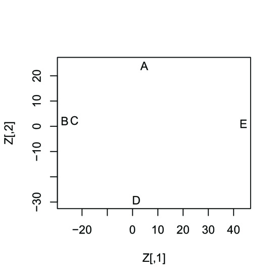
Figure 1: Two-dimensional MDS solution for train journey times between 5 rail stations in Yorkshire. A: Leeds, B: Headingley, C: Horsforth, D: Harrogate, E: York.

The eigenvalues of $\mathbf{B}$ are

$$\lambda_{1}=3210,\lambda_{2}=1439,\lambda_{3}=61,\lambda_{4}=0,\lambda_{5}=-964,$$

and the corresponding eigenvectors in $\mathbf{\Gamma}$ are

Eigenvectors
      [,1]  [,2]  [,3]  [,4]  [,5]
[1,]  0.08  0.63 -0.06 -0.45  0.63
[2,] -0.48  0.06 -0.66 -0.45 -0.38
[3,] -0.41  0.06  0.75 -0.45 -0.26
[4,]  0.03 -0.77 -0.04 -0.45  0.45
[5,]  0.77  0.02  0.00 -0.45 -0.45

We take our MDS solution to be the two dimensional principal coordinates. Figure 1 plots these two dimensional principal coordinates. Obviously as seen by the eigenvalues, $\mathbf{D}$ is not a distance matrix. Also we can check that

$$71=\delta_{25}>\delta_{12}+\delta_{15}=23+31=54,$$

which violates the triangle inequality.

The eigenvalues are 3210, 1439, 61, 0, -964. The first two are considerably larger than the rest in absolute value, suggesting the 2D MDS solutions should be a good representation. In particular, $\lambda_{3}=61$ seems negligible, $\lambda_{4}=0$ is an eigenvalue that always appears with eigenvector $\underaccent{\bar}{1}_{n}$, $\lambda_{5}=-964$ is smaller than the first two eigenvalues, but not entirely negligible and may cause some distortion in the reconstruction as we now examine.

Figure 1 shows that the stations lie roughly on a circle (not surprising since there are two lines between Leeds and York). Also, Headingley and Horsforth are close together, and Leeds is further from Harrogate than from York in terms of the dissimilarity though geographically Harrogate is nearer to Leeds than York.

In the MDS solution, the Euclidean distance between Headingley and Horsforth is 7.1, which is smaller than the dissimilarity value 11. On the other hand, in the MDS solution the Euclidean distance between Leeds and York is 45.5, which is larger than the dissimilarity value 31. We can now explain this behaviour using the spectral decomposition of $\mathbf{B}$, and using the result derived in this section. Let us now denote the stations A, $\ldots$, E by $1,\ldots,5$ respectively. Eigenvector entries for selected stations (and the corresponding eigenvalues 61 and -964 respectively)
Station $j=3$ $j=5$ Headingley (2) -0.66 -0.38 Horsforth (3) 0.75 -0.26 absolute difference 1.41 0.12 Leeds (1) -0.06 0.63 York (5) 0.00 -0.45 absolute difference 0.06 1.08

Hence, the difference between Headingley and Horsforth is dominated by the eigenvector $j=3$ (with positive eigenvalue, 61), whereas the difference between Leeds and York is dominated by the eigenvector $j=5$ (with negative eigenvalue, -964). In fact, the numerical values of the terms (26) in the difference between the two distances given by (29) are

$$g_{23}^{(3)}=121.3,\quad g_{23}^{(4)}=0,\quad g_{23}^{(5)}=-13.9,$$

and

$$g_{15}^{(3)}=0.2,\quad g_{15}^{(4)}=0,\quad g_{15}^{(5)}=-1124.4,$$

so the dominated contributions $g_{23}^{(3)}$ and $g_{15}^{(5)}$ are clearly seen. This discussion explains why in the MDS solution, the Euclidean distance between Headingley (2) and Horsforth (3) is smaller than the dissimilarity value whereas the Euclidean distance between Leeds (1) and York (5) is larger than the dissimilarity value.

5 Acknowledgment

We wish to express our thanks to Wally Gilks and John Kent for their helpful comments and to the University of Leeds for the Example in Section 4 from an Examination paper. The first author would also like to thank the Leverhulme Trust for the Emeritus Fellowship.

6 References

Mardia, K. V., Kent, J. T., and Bibby, J. M. (1979). Multivariate Analysis. Academic press.