Semantic Feature Extraction for Generalized Zero-shot Learning
Abstract
Generalized zero-shot learning (GZSL) is a technique to train a deep learning model to identify unseen classes using the attribute. In this paper, we put forth a new GZSL technique that improves the GZSL classification performance greatly. Key idea of the proposed approach, henceforth referred to as semantic feature extraction-based GZSL (SE-GZSL), is to use the semantic feature containing only attribute-related information in learning the relationship between the image and the attribute. In doing so, we can remove the interference, if any, caused by the attribute-irrelevant information contained in the image feature. To train a network extracting the semantic feature, we present two novel loss functions, 1) mutual information-based loss to capture all the attribute-related information in the image feature and 2) similarity-based loss to remove unwanted attribute-irrelevant information. From extensive experiments using various datasets, we show that the proposed SE-GZSL technique outperforms conventional GZSL approaches by a large margin.
Introduction
Image classification is a long-standing yet important task with a wide range of applications such as autonomous driving, industrial automation, medical diagnosis, and biometric identification (Fujiyoshi, Hirakawa, and Yamashita 2019; Ren, Hung, and Tan 2017; Ronneberger, Fischer, and Brox 2015; Sun et al. 2013). In solving the task, supervised learning (SL) techniques have been popularly used for its superiority (Simonyan and Zisserman 2014; He et al. 2016). Well-known drawback of SL is that a large number of training data are required for each and every class to be identified. Unfortunately, in many practical scenarios, it is difficult to collect training data for certain classes (e.g., endangered species and newly observed species such as variants of COVID-19). When there are unseen classes where training data is unavailable, SL-based models are biased towards the seen classes, impeding the identification of the unseen classes.
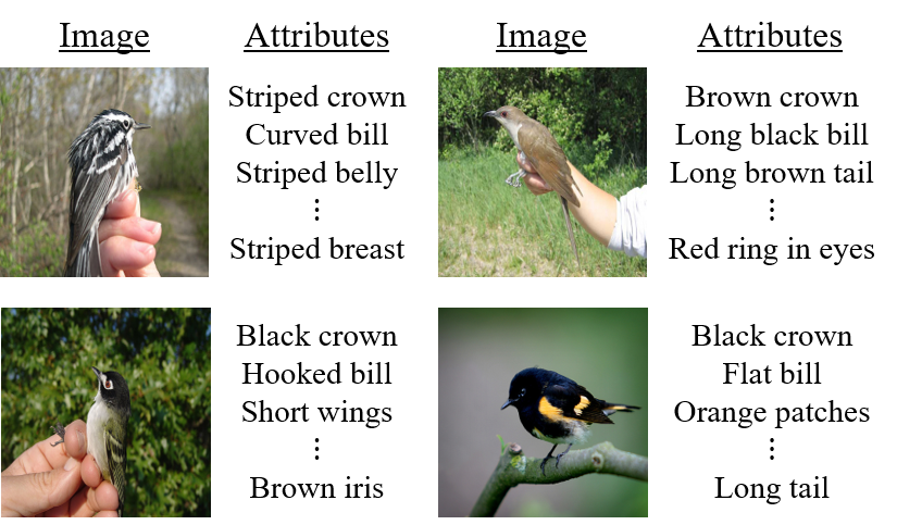
Recently, to overcome this drawback, a technique to train a classifier using manually annotated attributes (e.g., color, size, and shape; see Fig. 1) has been proposed (Lampert, Nickisch, and Harmeling 2009; Chao et al. 2016). Key idea of this technique, dubbed as generalized zero-shot learning (GZSL), is to learn the relationship between the image and the attribute from seen classes and then use the trained model in the identification of unseen classes. In (Akata et al. 2015), for example, an approach to identify unseen classes by measuring the compatibility between the image feature and attribute has been proposed. In (Mishra et al. 2018), a network synthesizing the image feature from the attribute has been employed to generate training data of unseen classes. In extracting the image feature, a network trained using the classification task (e.g., ResNet (He et al. 2016)) has been popularly used. A potential drawback of this extraction method is that the image feature might contain attribute-irrelevant information (e.g., human fingers in Fig. 1), disturbing the process of learning the relationship between the image and the attribute (Tong et al. 2019; Han, Fu, and Yang 2020; Li et al. 2021).
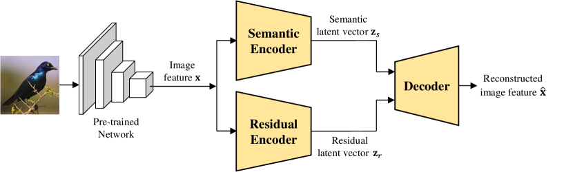
In this paper, we propose a new GZSL technique that removes the interference caused by the attribute-irrelevant information. Key idea of the proposed approach is to extract the semantic feature, feature containing the attribute-related information, from the image feature and then use it in learning the relationship between the image and the attribute. In extracting the semantic feature, we use a modified autoencoder consisting of two encoders, viz., semantic and residual encoders (see Fig. 2). In a nutshell, the semantic encoder captures all the attribute-related information in the image feature and the residual encoder catches the attribute-irrelevant information.
In the conventional autoencoder, only reconstruction loss (difference between the input and the reconstructed input) is used for the training. In our approach, to encourage the semantic encoder to capture the attribute-related information only, we use two novel loss functions on top of the reconstruction loss. First, we employ the mutual information (MI)-based loss to maximize (minimize) MI between the semantic (residual) encoder output and the attribute. Since MI is a metric to measure the level of dependency between two random variables, by exploiting the MI-based loss, we can encourage the semantic encoder to capture the attribute-related information and at the same time discourage the residual encoder to capture any attribute-related information. As a result, all the attribute-related information can be solely captured by the semantic encoder. Second, we use the similarity-based loss to enforce the semantic encoder not to catch any attribute-irrelevant information. For example, when a bird image contains human fingers (see Fig. 1), we do not want features related to the finger to be included in the semantic encoder output. To do so, we maximize the similarity between the semantic encoder outputs of images that are belonging to the same class (bird images in our example). Since attribute-irrelevant features are contained only in a few image samples (e.g., human fingers are included in a few bird images), by maximizing the similarity between the semantic encoder outputs of the same class, we can remove attribute-irrelevant information from the semantic encoder output.
From extensive experiments using various benchmark datasets (AwA1, AwA2, CUB, and SUN), we demonstrate that the proposed approach outperforms the conventional GZSL techniques by a large margin. For example, for the AwA2 and CUB datasets, our model achieves 2% improvement in the GZSL classification accuracy over the state-of-the-art techniques.
Related Work and Background
Conventional GZSL Approaches
The main task in GZSL is to learn the relationship between the image and the attribute from seen classes and then use it in the identification of unseen classes. Early GZSL works have focused on the training of a network measuring the compatibility score between the image feature and the attribute (Akata et al. 2015; Frome et al. 2013). Once the network is trained properly, images can be classified by identifying the attribute achieving the maximum compatibility score. Recently, generative model-based GZSL approaches have been proposed (Mishra et al. 2018; Xian et al. 2018). Key idea of these approaches is to generate synthetic image features of unseen classes from the attributes by employing a generative model (Mishra et al. 2018; Xian et al. 2018). As a generative model, conditional variational autoencoder (CVAE) (Kingma and Welling 2013) and conditional Wasserstein generative adversarial network (CWGAN) (Arjovsky, Chintala, and Bottou 2017) have been popularly used. By exploiting the generated image features of unseen classes as training data, a classification network identifying unseen classes can be trained in a supervised manner.
Over the years, many efforts have been made to improve the performance of the generative model. In (Xian et al. 2019; Schonfeld et al. 2019; Gao et al. 2020), an approach to combine multiple generative models (e.g., CVAE and CWGAN) has been proposed. In (Felix et al. 2018; Ni, Zhang, and Xie 2019), an additional network estimating the image attribute from the image feature has been used to make sure that the synthetic image features satisfy the attribute of unseen classes. In (Xian et al. 2018; Vyas, Venkateswara, and Panchanathan 2020; Li et al. 2019), an additional image classifier has been used in the generative model training to generate distinct image features for different classes.
Our approach is conceptually similar to the generative model-based approach in the sense that we generate synthetic image features of unseen classes using the generative model. The key distinctive point of the proposed approach over the conventional approaches is that we use the features containing only attribute-related information in the classification to remove the interference, if any, caused by the attribute-irrelevant information.
MI for Deep Learning
Mathematically, the MI between two random variables and is defined as
| (1) |
where is the joint probability density function (PDF) of and , and and are marginal PDFs of and , respectively. In practice, it is very difficult to compute the exact value of MI since the joint PDF is generally unknown and the integrals in (1) are often intractable. To approximate MI, various MI estimators have been proposed (Oord, Li, and Vinyals 2018; Cheng et al. 2020). Representative estimators include InfoNCE (Oord, Li, and Vinyals 2018) and contrastive log-ratio upper bound (CLUB) (Cheng et al. 2020), defined as
| (2) | ||||
| (3) |
where is a pre-defined score function measuring the compatibility between and , and is the conditional PDF of given , which is often approximated by a neural network.
The relationship between MI, InfoNCE, and CLUB is given by
| (4) |
Recently, InfoNCE and CLUB have been used to strengthen or weaken the independence between different parts of the neural network. For example, when one tries to enforce the independence between and , that is, to reduce , an approach to minimize the upper bound of MI can be used (Yuan et al. 2021). Whereas, when one wants to maximize the dependence between and , that is, to increase , an approach to maximize the lower bound of MI (Tschannen et al. 2019) can be used.
SE-GZSL
In this section, we present the proposed GZSL technique called semantic feature extraction-based GZSL (SE-GZSL). We first discuss how to extract the semantic feature from the image feature and then delve into the GZSL classification using the extracted semantic feature.
Semantic Feature Extraction
In extracting the semantic feature from the image feature, the proposed SE-GZSL technique uses the modified autoencoder architecture where two encoders, called semantic and residual encoders, are used in capturing the attribute-related information and the attribute-irrelevant information, respectively (see Fig 2). As mentioned, in the autoencoder training, we use two loss functions: 1) MI-based loss to encourage the semantic encoder to capture all attribute-related information and 2) similarity-based loss to encourage the semantic encoder not to capture attribute-irrelevant information. In this subsection, we discuss the overall training loss with emphasis on these two.
MI-based Loss
To make sure that all the attribute-related information is contained in the semantic encoder output, we use MI in the autoencoder training. To do so, we maximize MI between the semantic encoder output and the attribute which is given by manual annotation. At the same time, to avoid capturing of attribute-related information in the residual encoder, we minimize MI between the residual encoder output and the attribute. Let and be the semantic and residual encoder outputs corresponding to the image feature , and be the image attribute (see Fig. 2). Then, our training objective can be expressed as
| (5) |
where and () are weighting coefficients.
Since the computation of MI is not tractable, we use InfoNCE and CLUB (see (2) and (3)) as a surrogate of MI. In our approach, to minimize the objective function in (5), we express its upper bound using InfoNCE and CLUB and then train the autoencoder in a way to minimize the upper bound. Using the relationship between MI and its estimators in (4), the upper bound of the objective function in (5) is
| (6) |
Let be the set of seen classes, be the attribute of a seen class , and be the set of training image features for the class . Further, let and be the semantic and residual encoder outputs corresponding to the input image feature , respectively, then can be expressed as
| (7) |
where is the total number of training image features.
Similarity-based Loss
We now discuss the similarity-based loss to enforce the semantic encoder not to capture any attribute-irrelevant information.
Since images belonging to the same class have the same attribute, attribute-related image features of the same class would be more or less similar. This means that if the semantic encoder captures attribute-related information only, then the similarity between semantic encoder outputs of the same class should be large. Inspired by this observation, to remove the attribute-irrelevant information from the semantic encoder output, we train the semantic encoder in a way to maximize the similarity between outputs of the same class:
| (8) |
where the similarity is measured using the cosine-similarity function defined as
Also, we minimize the similarity between semantic encoder outputs of different classes to obtain sufficiently distinct semantic encoder outputs for different classes:
| (9) |
Using the fact that one can maximize and minimize at the same time by minimizing , we obtain the similarity-based loss as
| (10) |
Overall Loss
By adding the conventional reconstruction loss for the autoencoder, the MI-based loss , and the similarity-based loss , we obtain the overall loss function as
| (11) |
where is a weighting coefficient and is the reconstruction loss given by
| (12) |
Here, is the image feature reconstructed using the semantic and residual encoder outputs ( and ) in the decoder. When the training is finished, we only use the semantic encoder for the purpose of extracting the semantic feature.
GZSL Classification Using Semantic Features
So far, we have discussed how to extract the semantic feature from the image feature. We now discuss how to perform the GZSL classification using the semantic feature.
In a nutshell, we synthesize semantic feature samples for unseen classes from their attributes. Once the synthetic samples are generated, the semantic classifier identifying unseen classes from the semantic feature is trained in a supervised manner.
Semantic Feature Generation
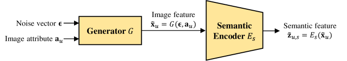
To synthesize the semantic feature samples for unseen classes, we first generate image features from the attributes of unseen classes and then extract the semantic features from the synthetic image features using the semantic encoder (see Fig. 3).
In synthesizing the image feature, we employ WGAN that mitigates the unstable training issue of GAN by exploiting a Wasserstein distance-based loss function (Arjovsky, Chintala, and Bottou 2017). The main component in WGAN is a generator synthesizing the image feature from a random noise vector and the image attribute (i.e., ). Conventionally, WGAN is trained to minimize the Wasserstein distance between the distributions of real image feature and generated image feature given by
| (13) | ||||
where is an auxiliary network (called critic), , and is the regularization coefficient (a.k.a., gradient penalty coefficient) (Gulrajani et al. 2017). In our scheme, to make sure that the semantic feature obtained from is similar to the real semantic feature , we additionally use the following losses in the WGAN training:
| (14) | ||||
| (15) |
We note that these losses are analogous to the losses with respect to the real semantic feature in (6) and (10), respectively. By combining (13), (14), and (15), we obtain the overall loss function as
| (16) |
where and are weighting coefficients.
After the WGAN training, we use the generator and the semantic encoder in synthesizing semantic feature samples of unseen classes. Specifically, for each unseen class , we generate the semantic feature by synthesizing the image feature using the generator and then exploiting it as an input to the semantic encoder (see Fig. 3):
| (17) |
By resampling the noise vector , a sufficient number of synthetic semantic features can be generated.
Semantic Feature-based Classification
After generating synthetic semantic feature samples for all unseen classes, we train the semantic feature classifier using a supervised learning model (e.g., softmax classifier, support vector machine, and nearest neighbor). Suppose, for example, that the softmax classifier is used as a classification model. Let be the set of synthetic semantic feature samples for the unseen class , then the semantic feature classifier is trained to minimize the cross entropy loss111We recall that is the set of semantic features for the seen class .
| (18) |
where
| (19) |
and and are weight and bias parameters of the softmax classifier to be learned.
Comparison with Conventional Approaches
There have been previous efforts to extract the semantic feature from the image feature (Tong et al. 2019; Han, Fu, and Yang 2020; Li et al. 2021; Chen et al. 2021). While our approach seems to be a bit similar to (Li et al. 2021) and (Chen et al. 2021) in the sense that the autoencoder-based image feature decomposition method is used for the semantic feature extraction, our work is dearly distinct from those works in two respects. First, we use different training strategy in capturing the attribute-related information. In our approach, to make sure that the semantic encoder output contains all the attribute-related information, we use two complementary loss terms: 1) the loss term to encourage the semantic encoder to capture the attribute-related information and 2) the loss term to discourage the residual encoder to capture any attribute-related information (see (5)). Whereas, the training loss used to remove the attribute-related information from the residual encoder output has not been used in (Li et al. 2021; Chen et al. 2021). Also, we employ a new training loss to remove the attribute-irrelevant information from the semantic encoder output (see (10)), for which there is no counterpart in (Li et al. 2021; Chen et al. 2021).
Experiments
| Classifier input | AwA1 | AwA2 | CUB | SUN |
|---|---|---|---|---|
| Image feature | 90.9 | 92.8 | 73.8 | 47.1 |
| Semantic feature | 91.9 | 93.4 | 76.1 | 49.3 |
(a) Semantic features
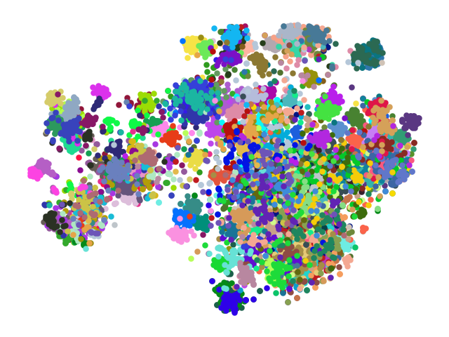
(b) Image features
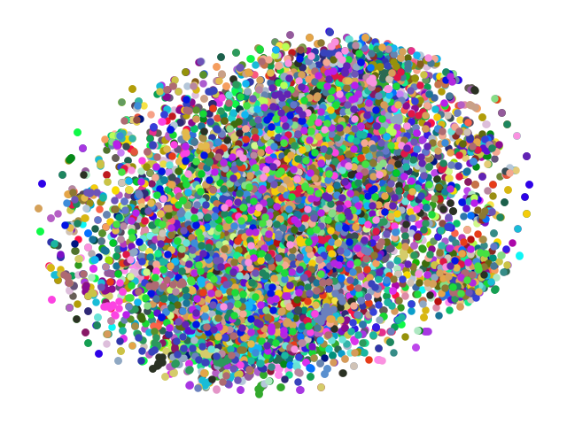
(c) Residual features
| Method | Feature Type | AwA1 | AwA2 | CUB | SUN | ||||||||
|---|---|---|---|---|---|---|---|---|---|---|---|---|---|
| CVAE-GZSL | ResNet | - | - | 47.2 | - | - | 51.2 | - | - | 34.5 | - | - | 26.7 |
| f-CLSWGAN | 61.4 | 57.9 | 59.6 | - | - | - | 57.7 | 43.7 | 49.7 | 36.6 | 42.6 | 39.4 | |
| cycle-CLSWGAN | 64.0 | 56.9 | 60.2 | - | - | - | 61.0 | 45.7 | 52.3 | 33.6 | 49.4 | 40.0 | |
| f-VAEGAN-D2 | - | - | - | 70.6 | 57.6 | 63.5 | 60.1 | 48.4 | 53.6 | 38.0 | 45.1 | 41.3 | |
| LisGAN | 76.3 | 52.6 | 62.3 | - | - | - | 57.9 | 46.5 | 51.6 | 37.8 | 42.9 | 40.2 | |
| CADA-VAE | 72.8 | 57.3 | 64.1 | 75.0 | 55.8 | 63.9 | 53.5 | 51.6 | 52.4 | 35.7 | 47.2 | 40.6 | |
| DASCN | 68.0 | 59.3 | 63.4 | - | - | - | 59.0 | 45.9 | 51.6 | 38.5 | 42.4 | 40.3 | |
| LsrGAN | 74.6 | 54.6 | 63.0 | - | - | - | 59.1 | 48.1 | 53.0 | 37.7 | 44.8 | 40.9 | |
| Zero-VAE-GAN | 66.8 | 58.2 | 62.3 | 70.9 | 57.1 | 62.5 | 47.9 | 43.6 | 45.5 | 30.2 | 45.2 | 36.3 | |
| DLFZRL | Semantic | - | - | 61.2 | - | - | 60.9 | - | - | 51.9 | - | - | 42.5 |
| RFF-GZSL | 75.1 | 59.8 | 66.5 | - | - | - | 56.6 | 52.6 | 54.6 | 38.6 | 45.7 | 41.9 | |
| Disentangled-VAE | 72.9 | 60.7 | 66.2 | 80.2 | 56.9 | 66.6 | 58.2 | 51.1 | 54.4 | 36.6 | 47.6 | 41.4 | |
| SE-GZSL | Semantic | 76.7 | 61.3 | 68.1 | 80.7 | 59.9 | 68.8 | 60.3 | 53.1 | 56.4 | 40.7 | 45.8 | 43.1 |
| Loss | AwA1 | AwA2 | CUB | SUN | ||||||||
|---|---|---|---|---|---|---|---|---|---|---|---|---|
| 64.6 | 53.1 | 58.3 | 68.9 | 55.7 | 61.6 | 54.5 | 46.1 | 49.9 | 38.4 | 40.6 | 39.4 | |
| + | 75.0 | 57.9 | 65.4 | 74.2 | 58.6 | 65.5 | 59.4 | 51.5 | 55.1 | 37.1 | 46.5 | 41.3 |
| + + | 76.7 | 61.3 | 68.1 | 80.7 | 59.9 | 68.8 | 60.3 | 53.1 | 56.4 | 40.7 | 45.8 | 43.1 |
Experimental Setup
Datasets
In our experiments, we evaluate the performance of our model using four benchmark datasets: AwA1, AwA2, CUB, and SUN. The AwA1 and AwA2 datasets contain 50 classes of animal images annotated with 85 attributes (Lampert, Nickisch, and Harmeling 2009; Xian, Schiele, and Akata 2017). The CUB dataset contains 200 species of bird images annotated with 312 attributes (Welinder et al. 2010). The SUN dataset contains 717 classes of scene images annotated with 102 attributes (Patterson and Hays 2012). In dividing the total classes into seen and unseen classes, we adopt the conventional dataset split presented in (Xian, Schiele, and Akata 2017).
Implementation Details
As in (Xian et al. 2018; Schonfeld et al. 2019), we use ResNet-101 (He et al. 2016) as a pre-trained classification network and fix it in our training process. We implement all the networks in SE-GZSL (semantic encoder, residual encoder, and decoder in the image feature decomposition network, and generator and critic in WGAN) using the multilayer perceptron (MLP) with one hidden layer as in (Xian et al. 2018, 2019). We set the number of hidden units to 4096 and use LeakyReLU with a negative slope of 0.02 as a nonlinear activation function. For the output layer of the generator, the ReLU activation is used since the image feature extracted by ResNet is non-negative. As in (Oord, Li, and Vinyals 2018), we define the score function in (6) as where is a weight matrix to be learned. Also, as in (Cheng et al. 2020), we approximate the conditional PDF in (6) using a variational encoder consisting of two hidden layers. The gradient penalty coefficient in the WGAN loss is set to as suggested in the original WGAN paper (Gulrajani et al. 2017). We set the weighting coefficients in (7), (11), and (16) to .
Semantic Feature-based Image Classification
We first investigate whether the image classification performance can be improved by exploiting the semantic feature. To this end, we train two image classifiers: the classifier exploiting the image feature and the classifier utilizing the semantic feature extracted by the semantic encoder. To compare the semantic feature directly with the image feature, we use the simple softmax classifier as a classification model. In Table 1, we summarize the top-1 classification accuracy of each classifier on test image samples for seen classes. We observe that the semantic feature-based classifier outperforms the image feature-based classifier for all datasets. In particular, for the SUN and CUB datasets, the semantic feature-based classifier achieves about improvement in the top-1 classification accuracy over the image feature-based classifier, which demonstrates that the image classification performance can be enhanced by removing the attribute-irrelevant information in the image feature.
Visualization of Semantic Features
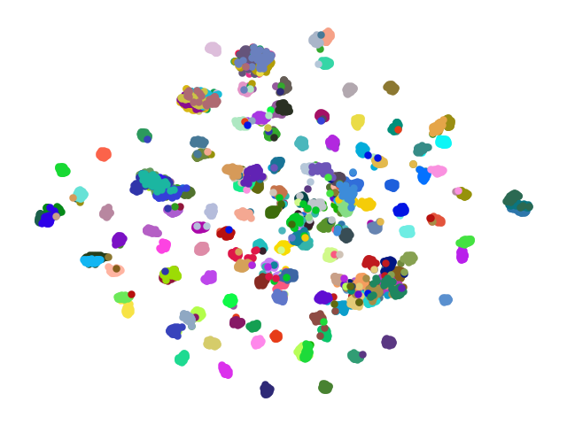
In Fig. 4, we visualize semantic feature samples obtained from the CUB dataset using a t-distributed stochastic neighbor embedding (t-SNE), a tool to visualize high-dimensional data in a two-dimensional plane (Van der Maaten and Hinton 2008). For comparison, we also visualize image feature samples and residual feature samples extracted by the residual encoder. We observe that semantic feature samples containing only attribute-related information are well-clustered, that is, samples of the same class are grouped and samples of different classes are separated (see Fig. 4(a)). Whereas, image feature samples of different classes are not separated sufficiently (see Fig. 4(b)) and residual feature samples are scattered randomly (see Fig. 4(c)).
Comparison with State-of-the-art
We next evaluate the GZSL classification performance of the proposed approach using the standard evaluation protocol presented in (Xian, Schiele, and Akata 2017). Specifically, we measure the average top-1 classification accuracies and on seen and unseen classes, respectively, and then use their harmonic mean as a metric to evaluate the performance. In Table 2, we summarize the performance of SE-GZSL on different datasets. For comparison, we also summarize the performance of conventional methods among which DLFZRL, RFF-GZSL, and Disentangled-VAE are semantic feature-based approaches (Tong et al. 2019; Han, Fu, and Yang 2020; Li et al. 2021) and other methods are image feature-based approaches (Mishra et al. 2018; Xian et al. 2018; Felix et al. 2018; Xian et al. 2019; Li et al. 2019; Schonfeld et al. 2019; Ni, Zhang, and Xie 2019; Vyas, Venkateswara, and Panchanathan 2020; Gao et al. 2020).
From the results, we observe that the proposed SE-GZSL outperforms conventional image feature-based approaches by a large margin. For example, for the AwA2 dataset, SE-GZSL achieves about 5% improvement in the harmonic mean accuracy over image feature-based approaches. We also observe that SE-GZSL outperforms existing semantic feature-based approaches for all datasets. For example, for the AwA1, AwA2, and CUB datasets, our model achieves about 2% improvement in the harmonic mean accuracy over the state-of-the-art approaches.
Ablation Study
Effectiveness of Loss Functions
In training the semantic feature extractor, we have used the MI-based loss and the similarity-based loss . To examine the impact of each loss function, we measure the performance of three different versions of SE-GZSL: 1) SE-GZSL trained only with the reconstruction loss , 2) SE-GZSL trained with and , and 3) SE-GZSL trained with , , and . From the results in Table 3, we observe that the performance of SE-GZSL can be enhanced greatly by exploiting the MI-based loss . In particular, for the AwA1 and CUB datasets, we achieve more than improvement in the harmonic mean accuracy by utilizing . Also, for the AwA2 dataset, we achieve about improvement of the accuracy. One might notice that when is not used, SE-GZSL performs worse than conventional image feature-based methods (see Table 2). This is because the semantic encoder cannot capture all the attribute-related information without , and thus using the semantic encoder output in the classification incurs the loss of the attribute-related information. We also observe that the performance of SE-GZSL can be improved further by exploiting the similarity-based loss . For example, for the AwA2 dataset, more than improvement in the harmonic mean accuracy can be achieved by utilizing .
Importance of Residual Encoder
| Method | AwA1 | AwA2 | CUB | SUN |
|---|---|---|---|---|
| SE-GZSL w/o residual encoder | 66.7 | 67.5 | 55.1 | 42.1 |
| SE-GZSL w/ residual encoder | 68.1 | 68.8 | 56.4 | 43.1 |
For the semantic feature extraction, we have decomposed the image feature into the attribute-related feature and the attribute-irrelevant feature using the semantic and residual encoders. An astute reader might ask why the residual encoder is needed to extract the semantic feature. To answer this question, we measure the performance of SE-GZSL without using the residual encoder. From the results in Table 4, we can observe that the GZSL performance of SE-GZSL is degraded when the residual encoder is not used. This is because if the residual encoder is removed, then the attribute-irrelevant information, required for the reconstruction of the image feature, would be contained in the semantic encoder output and therefore mess up the process to learn the relationship between the image feature and the attribute.
Conclusion
In this paper, we presented a new GZSL technique called SE-GZSL. Key idea of the proposed SE-GZSL is to exploit the semantic feature in learning the relationship between the image and the attribute, removing the interference caused by the attribute-irrelevant information. To extract the semantic feature, we presented the autoencoder-based image feature decomposition network consisting of semantic and residual encoders. In a nutshell, the semantic and residual encoders capture the attribute-related information and the attribute-irrelevant information, respectively. In training the image feature decomposition network, we used MI-based loss to encourage the semantic encoder to capture all the attribute-related information and similarity-based loss to discourage the semantic encoder to capture any attribute-irrelevant information. Our experiments on various datasets demonstrated that the proposed SE-GZSL outperforms conventional GZSL approaches by a large margin.
Acknowledgements
This work was supported in part by the Samsung Research Funding & Incubation Center for Future Technology of Samsung Electronics under Grant SRFC-IT1901-17 and in part by the National Research Foundation of Korea (NRF) grant funded by the Korea government (MSIT) under Grant 2020R1A2C2102198.
References
- Akata et al. (2015) Akata, Z.; Perronnin, F.; Harchaoui, Z.; and Schmid, C. 2015. Label-Embedding for Image Classification. IEEE Transactions on Pattern Analysis and Machine Intelligence, 38(7): 1425–1438.
- Arjovsky, Chintala, and Bottou (2017) Arjovsky, M.; Chintala, S.; and Bottou, L. 2017. Wasserstein Generative Adversarial Networks. In Proceedings of the International Conference on Machine Learning, 214–223.
- Chao et al. (2016) Chao, W.-L.; Changpinyo, S.; Gong, B.; and Sha, F. 2016. An Empirical Study and Analysis of Generalized Zero-Shot Learning for Object Recognition in the Wild. In Proceedings of the European Conference on Computer Vision, 52–68.
- Chen et al. (2021) Chen, Z.; Luo, Y.; Qiu, R.; Wang, S.; Huang, Z.; Li, J.; and Zhang, Z. 2021. Semantics Disentangling for Generalized Zero-Shot Learning. In Proceedings of the IEEE/CVF International Conference on Computer Vision, 8712–8720.
- Cheng et al. (2020) Cheng, P.; Hao, W.; Dai, S.; Liu, J.; Gan, Z.; and Carin, L. 2020. CLUB: A Contrastive Log-ratio Upper Bound of Mutual Information. In Proceedings of the International Conference on Machine Learning, 1779–1788.
- Felix et al. (2018) Felix, R.; Reid, I.; Carneiro, G.; et al. 2018. Multi-Modal Cycle-Consistent Generalized Zero-Shot Learning. In Proceedings of the European Conference on Computer Vision, 21–37.
- Frome et al. (2013) Frome, A.; Corrado, G.; Shlens, J.; Bengio, S.; Dean, J.; Ranzato, M.; and Mikolov, T. 2013. DeViSE: A Deep Visual-Semantic Embedding Model. In Proceedings of the International Conference on Neural Information Processing Systems, 2121–2129.
- Fujiyoshi, Hirakawa, and Yamashita (2019) Fujiyoshi, H.; Hirakawa, T.; and Yamashita, T. 2019. Deep Learning-based Image Recognition for Autonomous Driving. IATSS Research, 43(4): 244–252.
- Gao et al. (2020) Gao, R.; Hou, X.; Qin, J.; Chen, J.; Liu, L.; Zhu, F.; Zhang, Z.; and Shao, L. 2020. Zero-VAE-GAN: Generating Unseen Features for Generalized and Transductive Zero-Shot Learning. IEEE Transactions on Image Processing, 29: 3665–3680.
- Gulrajani et al. (2017) Gulrajani, I.; Ahmed, F.; Arjovsky, M.; Dumoulin, V.; and Courville, A. 2017. Improved Training of Wasserstein GANs. In Proceedings of the International Conference on Neural Information Processing Systems, 5769–5779.
- Han, Fu, and Yang (2020) Han, Z.; Fu, Z.; and Yang, J. 2020. Learning the Redundancy-Free Features for Generalized Zero-Shot Object Recognition. In Proceedings of the IEEE/CVF Conference on Computer Vision and Pattern Recognition, 12865–12874.
- He et al. (2016) He, K.; Zhang, X.; Ren, S.; and Sun, J. 2016. Deep Residual Learning for Image Recognition. In Proceedings of the IEEE Conference on Computer vision and Pattern Recognition, 770–778.
- Kingma and Welling (2013) Kingma, D. P.; and Welling, M. 2013. Auto-Encoding Variational Bayes. arXiv:1312.6114.
- Lampert, Nickisch, and Harmeling (2009) Lampert, C. H.; Nickisch, H.; and Harmeling, S. 2009. Learning to Detect Unseen Object Classes by Between-Class Attribute Transfer. In Proceedings of the IEEE Conference on Computer Vision and Pattern Recognition, 951–958. IEEE.
- Li et al. (2019) Li, J.; Jing, M.; Lu, K.; Ding, Z.; Zhu, L.; and Huang, Z. 2019. Leveraging the Invariant Side of Generative Zero-Shot Learning. In Proceedings of the IEEE/CVF Conference on Computer Vision and Pattern Recognition, 7402–7411.
- Li et al. (2021) Li, X.; Xu, Z.; Wei, K.; and Deng, C. 2021. Generalized Zero-Shot Learning via Disentangled Representation. In Proceedings of the AAAI Conference on Artificial Intelligence, volume 35, 1966–1974.
- Mishra et al. (2018) Mishra, A.; Krishna Reddy, S.; Mittal, A.; and Murthy, H. A. 2018. A Generative Model for Zero Shot Learning Using Conditional Variational Autoencoders. In Proceedings of the IEEE Conference on Computer Vision and Pattern Recognition Workshops, 2188–2196.
- Ni, Zhang, and Xie (2019) Ni, J.; Zhang, S.; and Xie, H. 2019. Dual Adversarial Semantics-Consistent Network for Generalized Zero-Shot Learning. Advances in Neural Information Processing Systems, 32: 6146–6157.
- Oord, Li, and Vinyals (2018) Oord, A. v. d.; Li, Y.; and Vinyals, O. 2018. Representation Learning With Contrastive Predictive Coding. arXiv:1807.03748.
- Patterson and Hays (2012) Patterson, G.; and Hays, J. 2012. Sun Attribute Database: Discovering, Annotating, and Recognizing Scene Attributes. In Proceedings of the IEEE Conference on Computer Vision and Pattern Recognition, 2751–2758.
- Ren, Hung, and Tan (2017) Ren, R.; Hung, T.; and Tan, K. C. 2017. A Generic Deep-Learning-based Approach for Automated Surface Inspection. IEEE Transactions on Cybernetics, 48(3): 929–940.
- Ronneberger, Fischer, and Brox (2015) Ronneberger, O.; Fischer, P.; and Brox, T. 2015. U-net: Convolutional Networks for Biomedical Image Segmentation. In International Conference on Medical Image Computing and Computer-Assisted Intervention, 234–241. Springer.
- Schonfeld et al. (2019) Schonfeld, E.; Ebrahimi, S.; Sinha, S.; Darrell, T.; and Akata, Z. 2019. Generalized Zero-and Few-Shot Learning via Aligned Variational Autoencoders. In Proceedings of the IEEE/CVF Conference on Computer Vision and Pattern Recognition, 8247–8255.
- Simonyan and Zisserman (2014) Simonyan, K.; and Zisserman, A. 2014. Very Deep Convolutional Networks for Large-Scale Image Recognition. arXiv:1409.1556.
- Sun et al. (2013) Sun, Z.; Zhang, H.; Tan, T.; and Wang, J. 2013. Iris Image Classification Based on Hierarchical Visual Codebook. IEEE Transactions on Pattern Analysis and Machine Intelligence, 36(6): 1120–1133.
- Tong et al. (2019) Tong, B.; Wang, C.; Klinkigt, M.; Kobayashi, Y.; and Nonaka, Y. 2019. Hierarchical Disentanglement of Discriminative Latent Features for Zero-Shot Learning. In Proceedings of the IEEE/CVF Conference on Computer Vision and Pattern Recognition, 11467–11476.
- Tschannen et al. (2019) Tschannen, M.; Djolonga, J.; Rubenstein, P. K.; Gelly, S.; and Lucic, M. 2019. On Mutual Information Maximization for Representation Learning. arXiv:1907.13625.
- Van der Maaten and Hinton (2008) Van der Maaten, L.; and Hinton, G. 2008. Visualizing Data Using t-SNE. Journal of Machine Learning Research, 9(11).
- Vyas, Venkateswara, and Panchanathan (2020) Vyas, M. R.; Venkateswara, H.; and Panchanathan, S. 2020. Leveraging Seen and Unseen Semantic Relationships for Generative Zero-Shot Learning. In Proceedings of the European Conference on Computer Vision, 70–86.
- Welinder et al. (2010) Welinder, P.; Branson, S.; Mita, T.; Wah, C.; Schroff, F.; Belongie, S.; and Perona, P. 2010. Caltech-UCSD Birds 200.
- Xian et al. (2018) Xian, Y.; Lorenz, T.; Schiele, B.; and Akata, Z. 2018. Feature Generating Networks for Zero-Shot Learning. In Proceedings of the IEEE Conference on Computer Vision and Pattern Recognition, 5542–5551.
- Xian, Schiele, and Akata (2017) Xian, Y.; Schiele, B.; and Akata, Z. 2017. Zero-Shot Learning-the Good, the Bad and the Ugly. In Proceedings of the IEEE Conference on Computer Vision and Pattern Recognition, 4582–4591.
- Xian et al. (2019) Xian, Y.; Sharma, S.; Schiele, B.; and Akata, Z. 2019. f-VAEGAN-D2: A Feature Generating Framework for Any-Shot Learning. In Proceedings of the IEEE/CVF Conference on Computer Vision and Pattern Recognition, 10275–10284.
- Yuan et al. (2021) Yuan, S.; Cheng, P.; Zhang, R.; Hao, W.; Gan, Z.; and Carin, L. 2021. Improving Zero-shot Voice Style Transfer via Disentangled Representation Learning. arXiv:2103.09420.