Bayesian Neural Hawkes Process for Event Uncertainty Prediction

Abstract

Event data consisting of time of occurrence of the events arises in several real-world applications. Recent works have introduced neural network based point processes for modeling event-times, and were shown to provide state-of-the-art performance in predicting event-times. However, neural point process models lack a good uncertainty quantification capability on predictions. A proper uncertainty quantification over event modeling will help in better decision making for many practical applications. Therefore, we propose a novel point process model, Bayesian Neural Hawkes process (BNHP) which leverages uncertainty modelling capability of Bayesian models and generalization capability of the neural networks to model event occurrence times. We augment the model with spatio-temporal modeling capability where it can consider uncertainty over predicted time and location of the events. Experiments on simulated and real-world datasets show that BNHP significantly improves prediction performance and uncertainty quantification for modelling events.

1 Introduction

Many dynamic systems are characterized by sequences of discrete events over continuous time. Such temporal data are generated in various applications such as earthquakes, taxi-pickups, financial transactions, patient visits to hospitals etc. Despite these diverse domains, a common question across all the platforms is: Given an observed sequence of events, can we predict the time for the occurrence of the next event. A practical model should not only be capable of doing prediction but also model uncertainty in its predictions. For example, in healthcare predicting the patient arrival and uncertainty around prediction in the form of a time interval can help in queue management in hospitals. Similarly, uncertainty estimates for volcanic eruptions and earthquakes can help in risk management and make proactive decisions. A proper modelling of uncertainty will help users to determine what predictions by the event prediction model one can rely upon. Therefore, we need a model for event time prediction which can capture uncertainty. However, the neural models used for predicting temporal events make a point estimation of parameters and lack the required uncertainty modelling capability. This can lead to unreliable and overconfident predictions which can adversely affect decision making in many real-world applications. Therefore, we need to develop models which will also consider the confidence of the model in making the prediction.

Popular approaches for modeling event-data are based on point processes which are defined using a latent intensity function. A Hawkes process (HP) Hawkes (1971) is a point process with self-triggering property i.e. occurrences of previous events trigger occurrences of future events. A parametric form of the Hawkes process assumes monotonically decaying influence over past events, which may limit the expressive ability of the model and can deteriorate the performance on complex data sets. Therefore, recent techniques model the intensity function as a neural network Mei and Eisner (2017); Du et al. (2016); Xiao et al. (2017); Omi et al. (2019) so that the influence of past events can be modelled in a non-parametric manner without assuming a particular functional form.

Neural network based models typically tend to yield overconfident predictions and are incapable of properly modelling predictive uncertainty Gal (2016). This can be overcome by combining Bayesian principles in neural networks, leading to Bayesian neural networks (BNN) Neal (2012). BNN puts a distribution over the weight parameters and computes a posterior over them using Bayes theorem. Predictions are made using Bayesian model averaging using this posterior distribution which help in modelling uncertainty. However, determination of posterior is fraught with practical difficulties. Monte Carlo (MC) Dropout proposed by Gal and Ghahramani (2016a); Gal and Ghahramani (2016b) provides a practical and useful approach to develop BNNs. They proved that dropout regularization can be seen as equivalent to performing Bayesian inference over weights of a neural network.

In this paper, we propose Bayesian Neural Hawkes Process (BNHP) where we develop Monte Carlo dropout for a neural Hawkes process consisting of recurrent and feed-forward neural networks. BNHP is not only capable of modelling uncertainty but also improves the prediction of the event-times. Our contribution can be summarized as:

• We propose a novel model which combines the advantages of the neural Hawkes process and Bayesian neural network for modelling uncertainty over time of occurrence of events. We also extend the proposed approach to spatio-temporal event modeling set-up.

• We develop MC dropout for a neural Hawkes process network which consists of both recurrent and feed-forward neural networks.

• We demonstrate the effectiveness of BNHP for uncertainty modelling and prediction of event times and locations on several simulated and real world data.

2 Related Work

Hawkes process: Point processes Valkeila (2008) are useful to model the distribution of points and are defined using an underlying intensity function. Hawkes process Hawkes (1971) is a point process Valkeila (2008) with self-triggering property. i.e occurrence of previous events trigger occurrences of future events. Hawkes process has been used in earthquake modelling Hainzl et al. (2010), crime forecasting Mohler et al. (2011), finance Bacry et al. (2015); Embrechts et al. (2011) and epidemic forecasting Diggle et al. (2005); Chiang et al. (2021). However, to avoid parametric models various research works have proposed Du et al. (2016); Mei and Eisner (2017); Omi et al. (2019); Zuo et al. (2020) where intensity function is learnt using neural networks, which are better at learning unknown distributions. Along the direction of the spatio-temporal Hawkes process, Du et al. (2016) has considered spatial attributes by discretizing space and considering them as marks, which is unable to model spatio-temporal intensity function. Okawa et al. (2019); Zhou et al. (2021) has proposed spatio-temporal intensity as a mixture of kernels. Chen et al. (2020) has proposed Neural ODE for modeling spatio-temporal point processes. Another work Ilhan and Kozat (2020) has applied random Fourier features based transformations to represent kernel operations in spatio-temporal Hawkes process. A recent work Zhou et al. (2021) has introduced deep spatio-temporal point process where they integrate spatio-temporal point process with deep learning by modeling space-time intensity function as mixture of kernels where intensity is inferred using variational inference.

Bayesian Neural Networks (BNNs) Neal (2012); Gal (2016) are widely used framework to find uncertainty estimates for deep models. However, one has to resort to approximate inference techniques Graves (2011); Neal (2012) due to intractable posterior in BNNs. An alternative solution is to incorporate uncertainty directly into the loss function Lakshminarayanan et al. (2017); Pearce et al. (2018). Monte Carlo Dropout proposed by Gal and Ghahramani (2016a); Gal and Ghahramani (2016b) proved that dropout regularization Srivastava et al. (2014) can act as approximation for Bayesian inference over the weights of neural networks.

There are few works Zhang et al. (2020, 2019); Wang et al. (2020) where uncertainty is captured over the parameters of parametric hawkes process. In Chapfuwa et al. (2020) authors have proposed an adversarial non-parametric model that accounts for calibration and uncertainty for time to event and uncertainty prediction. However, neural point processes are a widely adopted model for event modeling due to its theoretical and practical effectiveness in various applications. Therefore, the goal of this paper is to augment the capabilities of the neural point process to predict future events with the uncertainty estimation capability. To achieve this, we propose a novel approach which combines neural point process and Monte Carlo dropout for performing uncertainty estimation for event-time prediction.

3 Bayesian Neural Hawkes Process

We consider the input sequence $S=\{t_{i}\}_{i=1}^{N}$ in the observation interval $[0,T]$ and inter-event time interval as $\tau_{i}=t_{i}-t_{i-1}$. Our goal is to predict the time of occurrence of next events along with uncertainty estimates over the predicted time. We consider a neural Hawkes process (NHP) Omi et al. (2019), which consider a combination of recurrent neural network and feed-forward neural network to model the likelihood associated with the sequence of events $\{t_{i}\}_{i=1}^{N}$ and predict the future events. We propose Bayesian Neural Hawkes process by developing MC dropout jointly over recurrent and feed-forward neural networks in an NHP.

3.1 Neural Hawkes Process

A major characteristic of the Hawkes process Hawkes (1971) is the conditional intensity function which conditions the next event occurrence based on the history of events. Following recent advances in Hawkes process Du et al. (2016); Omi et al. (2019), neural Hawkes processes were proposed which model the intensity function as a nonlinear function of history using a neural network. In particular Omi et al. (2019) uses a combination of recurrent neural network and feedforward neural network to model the intensity function. This allows the intensity function to take any functional form depending on data and help in better generalization performance. We represent history by using hidden representations generated by recurrent neural networks (RNNs) at each time step. The hidden representation $\boldsymbol{h}_{i}$ at time $t_{i}$ is obtained as

$$\boldsymbol{h}_{i}=RNN(\tau_{i},\boldsymbol{h}_{i-1};W_{r})=\sigma(\tau_{i}V_{r}+\boldsymbol{h}_{i-1}U_{r}+b_{r})$$ (1)

where $W_{r}$ represents the parameters associated with RNN such as input weight matrix $V^{r}$, recurrent weight matrix $U_{r}$, and and bias $b_{r}$. $\boldsymbol{h}_{i}$ is obtained by repeated application of the RNN block on a sequence formed from previous $M$ inter-arrival times. This is used as input to a feedforward neural network to compute the intensity function (hazard function) and consequently the cumulative hazard function for computing the likelihood of event occurrences.

In the proposed model, we consider the following input to the feed-forward neural network 1) the hidden representation generated from RNN, 2) time of occurrence of the event and 3) elapsed time from the most recent event. To better capture the uncertainty in predicting points in future time, we considered the time at which the intensity function needs to be evaluated. We model the conditional intensity as a function of the elapsed time from the most recent event, and is represented as $\lambda(t-t_{i}|\boldsymbol{h}_{i},t)$, where $\lambda(\cdot)$ is a non-negative function referred to as a hazard function. Therefore, we define cumulative hazard function in terms of inter-event interval

$$\tau=t-t_{i}=\Phi(\tau|\boldsymbol{h}_{i},t)=\int_{0}^{\tau}\lambda(s|\boldsymbol{h}_{i},t)ds$$ (2)

Cumulative hazard function is modeled using a feed-forward neural network (FNN)

$$\Phi(\tau|\boldsymbol{h}_{i},t)=FNN(\tau,h_{i},t;W_{t}).$$ (3)

However, we need to fulfill two properties of cumulative hazard function. Firstly, it has to be a monotonically increasing function of $\tau$ and secondly, it has to be positive valued. We achieve these by maintaining positive weights and positive activation functions in the neural network Chilinski and Silva (2020); Omi et al. (2019). The hazard function itself can be then obtained by differentiating the cumulative hazard function with respect to $\tau$ as

$$\lambda(\tau|\boldsymbol{h}_{i},t)=\frac{\partial}{\partial\tau}\Phi(\tau|\boldsymbol{h}_{i},t)$$ (4)

The log-likelihood of observing event times is defined as follows using the cumulative hazard function:

$$\begin{split}&\log p(\{t_{i}\}_{i=1}^{N};W)=\sum_{i=1}^{N}\log p(t_{i}|\mathcal{H}_{i};W)=\sum_{i=1}^{N}\big{(}\log(\frac{\partial}{\partial\tau}\Phi(\tau_{i}|\boldsymbol{h}_{i-1},t_{i};W))-\Phi(\tau_{i}|\boldsymbol{h}_{i-1},t_{i};W)\big{)}\end{split}$$ (5)

where $\tau_{i}=t_{i}-t_{i-1}$ and $W=\{W_{r},W_{t}\}$ represents the combined weights associated with RNN and FNN. In NHP, the weights of the networks are learnt by maximizing the likelihood given by (LABEL:eq:log_lik_nhp). The gradient of the log-likelihood function is calculated using backpropagation.

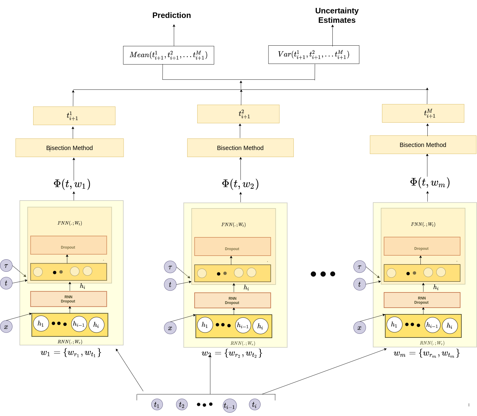
Figure 1: Framework for the proposed approach. Input: Time of occurrence associated with sequence of events. Output: time of occurrence of future events along with the uncertainty estimate.

3.2 Monte Carlo Dropout for Neural Hawkes Process

In this section, we discuss our proposed framework Bayesian Neural Hawkes Process (BNHP) (shown in Figure 1), for estimating uncertainty over time of occurrence of events. We propose a simple and practical approach based on Monte Carlo (MC) Dropout Gal and Ghahramani (2016a)] to model uncertainty in NHP. We develop MC Dropout for the NHP model which consists of two kinds of networks - RNN processing the input sequence and FNN producing the cumulative hazard function.

To model uncertainty, we follow a Bayesian approach, where we treat the weight matrices as random variables and put a prior distribution such as a standard Gaussian over them, i.e. $p(W)=\mathcal{N}(W;0,I)$. A Bayesian model will learn a posterior distribution over the parameters, instead of point estimates which allows them to capture uncertainty in the model. The likelihood of observing the event times given the weight parameters is defined by (LABEL:eq:log_lik_nhp). We find the posterior distribution over the parameters $p(W|\{t_{i}\}_{i=1}^{N})$ given the observed sequence of events using the Bayes Theorem,

$$p(W\mid\{t_{i}\}_{i=1}^{N})=\frac{p(\{t_{i}\}_{i=1}^{N}\mid W)p(W)}{p(\{t_{i}\}_{i=1}^{N})}.$$ (6)

However, the posterior computation is intractable due to non-linear functions modelled using neural networks. Hence, we find an approximate distribution $q(W)$ to the posterior $p(W|\{t_{i}\}_{i=1}^{N})$ using variational inference (VI) Blei et al. (2017). The parameters of $q(W)$ is obtained by minimizing the variational lower bound (ELBO) involving Kullback-Leibler (KL) divergence.

$$-\sum_{i=1}^{N}\int q(W)\,\log p(t_{i}|\mathcal{H}_{i};W)\,dW+KL(q(W)\parallel p(W))$$

Monte-Carlo (MC) dropout Gal and Ghahramani (2016a) assumes a particular form for the variational approximation which makes the ELBO computation equivalent to training the neural networks with dropout regularization. It has been shown that using VI with this specific form for the variational approximation is equivalent to applying dropout during training and testing Gal and Ghahramani (2016a).

A challenge with the neural Hawkes process in applying MC dropout is that, we have two kinds of neural networks with two types of weight parameters: $W_{t}$ associated with the FNN and $W_{r}$ associated with the RNN. Consequently, we use different variational approximations over each of the parameter types and thus different dropout regularizations as described below. We assume the variational distribution $q(W)$ can be decomposed as product of the variational distributions $q(W_{t})$ and $q(W_{r})$. We assume the following form for the variational distribution $q(W_{t})=\prod_{l=1}^{L}q(W_{t}^{l})$, where a sample $\hat{W}_{t}^{l}$ associated with layer $l$ is obtained from $q(W_{t}^{l})$ as

$$\hat{W}_{t}^{l}\sim\bar{W}_{t}^{l}\cdot diag([\mathbf{z}^{l}])\quad\,\quad\mathbf{z}^{l}\sim Bernoulli(p)$$ (7)

where $p$ is the drop probability and $\bar{W}_{t}^{l}$ are variational parameters (also weight matrix) to be estimated from the ELBO. Due to binary valued $\mathbf{z}^{l}$, $\hat{W}^{l}$ sampled from $q(W^{l})$ will have some of the columns of the weight matrix set to zero aiding in dropout regularization.

For the weights $W_{r}$ in the RNN , we use a variant of the standard MC-Dropout to perform learning and inference. First we assume the variational distribution $q(W_{r})$ to factorize over the weight matrices $V^{r}$, $U_{r}$, and $b_{r}$,

$$q(W_{r})=q(V_{r})q(U_{r})q(b_{r})$$ (8)

For each of these weight matrices, we assume the variational distribution to factorize over the rows,

$$q(V_{r})=\prod_{k=1}^{K}q(V_{rk})$$ (9)

Each row in the weight matrix follows an approximate distribution :

$$q(V_{rk})=p\mathcal{N}(V_{rk};0,\sigma_{r}^{2}I)+(1-p)\mathcal{N}(V_{rk};\bar{V}_{rk},\sigma_{r}^{2}I)$$ (10)

where $p$ is the drop probability, $\bar{V}_{rk}$ is the weight vector (also variational parameters) and $\sigma_{r}^{2}$ is the variance. The distribution (10) is similar to the sampling process in (7) when the variance is small. We sample the weight matrices $\hat{W}_{r}=\{\hat{V}_{r},\hat{U}_{r},\hat{b}_{r}\}$ associated with RNN from the variational distribution defined by (10). This results in the masking of random rows of the weight matrices. In the case of RNN, the same masked weight matrices are used for processing all the elements in the input sequence Gal and Ghahramani (2016b). But, different sequences use different masked weights.

For obtaining the distribution over the inter-arrival time $\tau_{i}$, we first obtain hidden representation $\mathbf{h}_{i-1}$ using an RNN with sampled weight matrices $\hat{W}_{ri}$. This is then fed through FNN along with other inputs and sampled weight matrix $\hat{W}_{ti}$ to obtain the cumulative hazard function $\Phi(\tau_{i}|\boldsymbol{h}_{i-1},t_{i},\hat{W}_{i})$. Consequently, the variational lower bound (ELBO) is written as

$$L_{VI}(\bar{W})=-\sum_{i=1}^{N}\log p(t_{i}|\mathcal{H}_{i};\hat{W}_{i})+\lambda\parallel\bar{W}\parallel^{2}$$

$$=-\sum_{i=1}^{N}\big{(}\log(\frac{\partial}{\partial\tau}\Phi(\tau_{i}|\boldsymbol{h}_{i-1},t_{i};\hat{W}_{i}))-\Phi(\tau_{i}|\boldsymbol{h}_{i-1},t_{i};\hat{W}_{i})\big{)}+\lambda(\parallel\bar{W}_{t}\parallel^{2}+\parallel\bar{V}_{r}\parallel^{2}+\parallel\bar{U}_{r}\parallel^{2}+\parallel\bar{b}_{r}\parallel^{2})$$

where $\bar{W}=\{\bar{W}_{t},\bar{V}_{r},\bar{U}_{r},\bar{b}_{r}\}$ represents all the weight matrices (variational parameters) that needs to be learnt by minimizing the objective function (3.2). We can observe that this is equivalent to learning weight parameters in a neural Hawkes process by minimizing the negative log-likelihood (LABEL:eq:log_lik_nhp), but with dropout regularization and $\ell_{2}$ norm regularization (obtained by simplifying the KL term) over the weight matrices.

3.3 Prediction and Uncertainty Estimation

For prediction, Bayesian models make use of the full posterior distribution over parameters rather than a point estimate of the parameters. This allows them to make robust predictions and model uncertainty over the predictions. After learning the variational parameters $\bar{W}$, we use the approximate posterior $q(W)$ to make predictions. The probability of predicting the time of next event given the history of previous event times with last event at $t_{N}$ is computed as

$$p(t_{*}|\mathcal{H})=\int p(t_{*}|\mathcal{H};W)q(W)dW=\frac{1}{S}\sum_{s=1}^{S}p(t_{*}|\mathcal{H};\hat{W}_{s})$$

where we approximated the integral with a Monte-Carlo approximation Neal (2012) with $S$ samples from $q(W)$ ($\hat{W}_{s}\sim q(W)$) and $\tau_{*}=t_{*}-t_{N}$. We can observe that sampling from $q(W)$ leads to performing dropout at the test time and the final prediction is obtained by averaging the prediction over multiple dropout architectures. Here, uncertainty in the weights induces model uncertainty for event time prediction.

Monte-Carlo dropout on NHP provides a feasible and practical technique to model uncertainty in event prediction. MC dropout is equivalent to performing $M$ forward passes through the NHP with stochastic dropouts at each layer but considering the specific nature of the network (recurrent or feedforward). Final prediction is done by taking an average prediction from the $M$ network architectures formed out of dropout in the forward pass. This can be seen as equivalent to ensemble of NHPs which could also lead to improved predictive performance. For each network, we use the bisection method Omi et al. (2019) to predict the time of the next event. Bisection method provides the median $t_{*}$ of the predictive distribution over next event time using the relation $\Phi(t_{*}-t_{N}|\boldsymbol{h}_{N},t_{*};\hat{W})=\log(2)$. We obtain $S$ median event times, with each median event time $t_{*_{s}}$ obtained using a network with sampled weight $\hat{W}_{s}$. The mean event time is then found by averaging $S$ times obtained from different sampled weights, $t_{*}=\frac{1}{S}\sum_{s=1}^{S}t_{*_{s}}$. The variance of predicted time is obtained as

$$Var(t_{*})={\sigma_{*}}^{2}=\frac{1}{S}\sum_{s=1}^{S}(t_{*_{s}}-t_{*})^{2}$$ (11)

We also define lower and upper bound of predicted time as

$${t}_{*}^{L}={t}_{*}-k\sigma_{*};\quad{t}_{*}^{U}={t}_{*}+k\sigma_{*}$$ (12)

Algorithm 1 provides the details of the prediction process, where $\hat{W}_{s}$ denotes a weight vector sample obtained using dropout at test time.

1:Input: $\{t_{1},t_{2},t_{3},\ldots,t_{p}\}$, number of MC samples $S$, parameters $W$ and neural HP network $f^{W}(\cdot)$ which consider previous $M$ inter-arrival times.

2:Output: Time of occurrence of future predictions $\hat{t}_{p+1},\hat{t}_{p+2},\ldots,\hat{t}_{n}$ and uncertainty intervals as $\{\hat{t}_{p+1}^{L}$, $\hat{t}_{p+1}^{U}\}$, $\{\hat{t}_{p+2}^{L}$, $\hat{t}_{p+2}^{U}\}$ and $\{\hat{t}_{n}^{L}$, $\hat{t}_{n}^{U}\}$

3:Train the model to learn $\bar{W}$ from the train data $\{t_{1},t_{2},t_{3},\ldots,t_{p}\}$ by minimizing the loss (3.2).

4:for $i\leftarrow p+1,n$ do

5:     for $s\leftarrow 1,S$ do

6:         $\Phi_{i}^{s}(\tau)\leftarrow f^{(\hat{W}_{s})}(\{\tau_{k},t_{k}\}_{k=i-M}^{i-1})$

7:         $\lambda_{i}^{s}(\tau)\leftarrow\frac{\partial}{\partial\tau}\Phi_{i}^{s}(\tau)$

8:         $\bar{t}_{i}^{(s)}\leftarrow\textsc{Bisection}(\Phi_{i}^{s}(\tau))$      

9:     $\hat{t}_{p}\leftarrow\frac{1}{S}\sum_{s=1}^{S}\bar{t}_{i}^{(s)}$

10:     $\sigma_{p}^{2}\leftarrow\frac{1}{S}\sum_{s=1}^{S}(\bar{t}_{p}^{(s)}-\hat{t}_{p})^{2}$

11:     $\hat{t}_{p}^{L}=\hat{t}_{p}-k*\sigma_{p}$, $\hat{t}_{p}^{U}=\hat{t}_{p}+k*\sigma_{p}$

Algorithm 1 Proposed Approach

3.4 Bayesian Neural Hawkes Process for Spatio-Temporal Modeling (ST-BNHP)

We extend the Bayesian Neural Hawkes Process developed for modeling uncertainty over time to modeling uncertainty over space. For applications involving spatio-temporal data such as traffic flow prediction, and human mobility prediction it is useful to obtain uncertainty over spatial points apart from the temporal uncertainty. Following Valkeila (2008), we model conditional intensity function for modelling the spatio-temporal data as $\lambda(t,x)=\lambda(t)p(\mathbf{x}|t)$, where $\mathbf{x}\in\mathcal{R}^{D}$ represents a spatial point or location and $p(\mathbf{x}|t)$ is the conditional spatial density of location $\mathbf{x}$ at t given $H_{t}$.

Since many mobility patterns involve movement in close-by regions, we model the conditional spatial density $p(\mathbf{x}_{i}|t_{i})$ as a Gaussian conditioned on the history, i.e. all the past events, times and locations ($(t_{i-},\mathbf{x}_{i-})$). Thus,

$$\begin{split}p(\mathbf{x}_{i}|t_{i-},\mathbf{x}_{i-})&=\mathcal{N}(\mathbf{x}_{i};\mu(t_{i-},\mathbf{x}_{i-}),\sigma(t_{i-},\mathbf{x}_{i-}))\end{split}$$ (13)

In the proposed model, we consider parameters of the Gaussian $\mu(\cdot)$ and $\sigma(\cdot)$ as functions of past event times and locations and are modeled using a feed-forward neural network.

$$[\mu(t_{i-},\mathbf{x}_{i-}),\sigma(t_{i-},\mathbf{x}_{i-})]=FNN(\boldsymbol{h}_{i},\mathbf{x}_{i-};W_{l})$$

where $\boldsymbol{h}_{i}$ is the hidden representation obtained from the RNN model with the sequence of the past event times as input.

The log likelihood for the spatio-temporal neural Hawkes model can be written as $\sum_{i=1}^{N}LL(t_{i},\mathbf{x}_{i};W,W_{l})$, where

$$LL(t_{i},\mathbf{x}_{i};W,W_{l})=\log p(t_{i}|\mathcal{H}_{i};W)+\log p(\mathbf{x}_{i}|t_{i-},x_{i-};W_{l}).$$

To obtain spatio-temporal Bayesian neural Hawkes (ST-BNHP) model, we consider a distribution over $W_{l}$ and follow a similar approach as in Section 3.2, where a variational distribution $q(W_{l})$ over $W_{l}$ is defined as in (7). The resulting ELBO considers the spatial likelihood and can be written as

$$\begin{split}&-\sum_{i=1}^{N}LL(t_{i},\mathbf{x}_{i};\hat{W}_{i},\hat{W}_{li})+\lambda(\parallel\bar{W}\parallel^{2}+\parallel\bar{W}_{l}\parallel^{2})\end{split}$$ (14)

where $\hat{W}_{li}\sim q(W_{l})$ and $\bar{W}_{l}$ is the variational parameter (weight matrix). The parameters are learnt by minimizing the lower bound (14) and is equivalent to learning with dropout regularization. Prediction is done as discussed in Section 3.2, where one considers multiple dropout architectures (corresponding to different samples of weight matrices), and taking an average over them. For each dropout architecture, we predict the time of occurrence of the next event using the bisection method and the location of of the next event by sampling from the conditional Gaussian $\mathcal{N}(\mathbf{x}_{*};\mu(t_{N-},\mathbf{x}_{N-}),\sigma(t_{N-},\mathbf{x}_{N-}))$.

		Sim-Poisson				Sim-Hawkes				Crime				Music
Metric	SHP	NHP	EH	BNHP	SHP	NHP	EH	BNHP	SHP	NHP	EH	BNHP	SHP	NHP	EH	BNHP
MNLL	1.21	1.36	*	0.196	1.08	1.26	*	0.166	1.809	1.42	*	0.279	1.239	0.97	*	-0.322
MAE	0.81	0.76	0.172	0.078	0.382	0.83	0.234	0.156	0.903	0.82	0.242	0.158	0.997	0.58	0.104	0.060
PIC@1	0.0	0.0	0.019	0.946	0.0	0.0	0.012	0.725	0.0	0.0	0.002	0.586	0.0	0.0	0.265	0.836
PIC@2	0.0	0.0	0.031	0.996	0.0	0.0	0.029	0.976	0.0	0.0	0.005	0.856	0.0	0.0	0.312	0.963
PIC@5	0.0	0.0	0.061	1.0	0.0	0.0	0.058	0.999	0.0	0.0	0.015	0.997	0.0	0.0	0.458	0.996

Table 1: Comparison of the proposed approach (BNHP) against the baselines (Please note that EH uses least square loss and hence MNLL for EH is not comparable to our results, hence MNLL for EH is marked with ’*’. )

Dataset	Method	MNLL	MNLL Temporal	MNLL Spatial	MAE time	MAE lat	MAE long	PIC time	PIC spatial
Foursquare	ST-HomogPoisson	8.204	-	-	4.229	1.23	1.824	0.026	0.025
	ST-NHP	5.366	1.562	3.804	2.048	0.889	0.798	0.0	0.387
	ST-BNHP	2.817	0.477	2.340	1.122	0.754	0.760	0.877	0.649
Taxi	ST-HomogPoisson	13.711	-	-	2.472	4.386	1.527	0.041	0.056
	ST-NHP	3.812	1.476	2.335	1.501	0.639	0.581	0.0	0.546
	ST-BNHP	2.392	0.054	2.338	0.133	0.589	0.536	0.386	0.721

Table 2: Comparison of the proposed approach (ST-BNHP) against the baselines for spatio-temporal modeling

Table 3: Dataset Statistics

Dataset	# events
Sim-Poisson	80,000
Sim-Hawkes	80,000
Crime	217,662
Music	112,610
NYC	200,000
Foursquare	95,702

4 Experiments and Results

Dataset Details

We extensively perform experiments on six datasets including two synthetic and four real-world datasets. Dataset statistics are mentioned in Table 3.

• Simulated Poisson (Sim-Poisson): We simulate a homogeneous poisson process with conditional intensity $\lambda$ = 1.

• Simulated Hawkes (Sim-Hawkes): We use the Hawkes process, in which the kernel function is given by the sum of multiple exponential functions. The conditional intensity function is given by $\lambda(t)=\mu+\sum_{t_{i}<t}\sum_{j=1}^{2}\alpha_{j}\beta_{j}\exp{(-\beta_{j}(t-t_{i}))}$. We have used $\mu=0.05$, $\alpha_{1}=0.4$, $\alpha_{2}=0.4$, $\beta_{1}=1.0$, $\beta_{1}=20.0$.

• Crime: This dataset contains the records of the police department calls for service in San Francisco . Each record contains the crime and timestamp associated with the call along with other information. We have selected ten such crimes as Burgalary, Drugs, Fraud, Injury, Accident, Intoxicated Person, Mentally disturbed, Person with knife, Stolen Vehicle, Suicide Attempt, Threats/Harrassment and their associated timestamps. Each sequence corresponds to a crime.

• Music: This dataset contains the history of music listening of users at lastfm . We consider 20 sequences from 20 most active users in the month of January, 2009. Each sequence corresponds to one user.

• New York Taxi: The dataset contains trip records for taxis in New York City. Each pick-up record is considered as an event. This datset contains spatial attributes in the form of latitude-longitude pair along with time of occurrence of events. We consider 100,000 events for each user and a sequence is constructed for each vendor.

• Foursquare: This is a location-based social network which contains information about check-ins of users. We have considered top 200 users during the period April 2012 to February, 2013. Each sequence corresponds to each user. This dataset also contains spatial attributes as latitude-longitude along with time of occurrence of events.

We have used the New York Taxi and Foursquare dataset for spatio-temporal modeling.

Evaluation metrics

We consider these metrics for evaluation of our results

• Mean Negative Log Likelihood (MNLL): Log-likelihood considers the probability of predicting the actual observations, and we expect a good model to have a lower MNLL score.

• Mean Absolute Error for prediction (MAE): The measure computes purely the absolute error in predicting the time without considering the probability. A model with low MAE will reflect a better model.

• Prediction Interval Coverage (PIC): It represents the number of times an actual event occurs within the estimated interval. Hence, higher PIC will represent a better model.

• Prediction Interval Length (PIL): It represents the length of difference between upper bound and lower bound of the predicted interval (Refer (12)). We report the mean and variance of interval length ($2*k*\sigma$). Higher PIL signifies more uncertainty associated with the event.

These evaluation metrics are tweaked for spatio-temporal modeling as well. For example, spatial MNLL represents conditional spatial density. MAE and PIL are calculated separately for latitude and longitude. Moreover, we modulate PIC in spatial manner by considering an actual event to occur within the estimated latitude and longitude bounds.

Baselines

We compare our experimental setup with the following baselines.

• NHP: Neural Hawkes process (NHP) Omi et al. (2019) serves as a baseline for evaluating the performance of predicted time of occurrence of event.

• SHP: We consider the standard Hawkes Process with exponential kernel as another baseline. NHP and SHP model probability distribution over event times $p(\tau|h_{i})$, though they do not model epistemic uncertainty like BNHP.

• Ensemble Hawkes (EH): We propose a new baseline capable of modelling epistemic uncertainty - an ensemble of parametric HP using exponential kernels with different hyper-parameters. To avoid convergence issues, we use least-square loss Xu et al. (2018) for training EH. Due to this, MNLL of EH won’t be comparable with other methods which use survival likelihood. Each ensemble consists of 10 models with decays ranging between 0.001 to 0.1.

• ST-HomogPoisson: The intensity is assumed to be constant over space and time. This is used as a baseline against ST-BNHP.

• ST-NHP: is the NHP augmented with the Gaussian spatial conditional density defined in (13).

Implementation Details

Herein, we present training details for all our experiments. We split our dataset into training, validation and test set as 70-10-20. The split is made across all sequences. Therefore, the first 70%, next 10% and last 20% of the events in each sequence are used for training, validation and testing respectively. The best hyperparameters are selected using the validation set. We consider a recurrent neural network with one layer and 64 units and 5-layer feed-forward neural network with 16 units in each layer. Recurrent Neural Network is associated with a dropout at input level as well as recurrent layer level. Along with that, there is a dropout associated with feedforward neural network to represent cumulative hazard function. Also, we use Tanh activation function. We use Adam optimizer with learning rate, $\beta_{1}$ and $\beta_{2}$ as 0.0001, 0.90 and 0.99 along with L2 regularization. We have used 50 different architectures using Monte Carlo Dropout. The results are reported after averaging the results after running the model three times. We perform 1-step lookahead prediction where we use actual time of occurrence of events as past events for the historical information to predict future event. We have perfomed all the experiments on Intel(R) Xeon(R) Silver 4208 CPU @ 2.10GHz, GeForce RTX 2080 Ti GPU and 128 GB RAM. We have implemented our code in Tensorflow 1.5.0 Abadi et al. (2015).

4.1 Results

We perform evaluation of the proposed methodology across quantitative and qualitative dimensions. We compare our results with the baselines and are reported in Table 1. We can observe that the proposed methodology is performing well in terms of time of prediction of event as well as uncertainty estimation for the event. The proposed method BNHP achieves significantly better MNLL and MAE as compared to NHP, SHP and ensemble of Hawkes Process for all the datasets. A better generalization performance can be attributed to the ensemble of NHP architectures obtained through dropout at test time. In addition to improved predictive performance, our approach also provides better uncertainty estimates. We quantify the uncertainty interval on the basis of how well the predicted intervals capture the actual occurrence of events. We report PIC@k in Table 1 for different values of k ($k=\{1,2,3\}$) in computing the upper bound and lower bound of the prediction interval(Refer (12)). SHP and NHP provide very small interval lengths and the actual points will not lie in this small interval, hence their PIC values are close to $0$. So, we compare the PIC of the proposed approach with an ensemble of Hawkes Processes. We can observe that we predict better PIC values compared to EH. We augment the proposed model to spatio-temporal event modeling as well where we predict uncertainty associated with time and location of the event. We report the results in Table 2. The proposed extension (ST-BNHP) performs better than both the baselines for both the datasets in terms of MNLL and MAE. We can observe that PIC@1 values are also better for predicted time and location (in terms of latitude and longitude) of occurrence of an event. One could argue that too wide intervals may yield higher PIC, but such intervals may be of no use. However, if the predicted intervals are too high, the algorithm will output higher MNLL score (or smaller log-likelihood). On the contrary, if the interval length is too small, then the number of events captured within the predicted interval will also be less, hence yielding a low PIC. Ideally, the length of the uncertainty interval should be large enough to capture points well and small enough to yield low MNLL. We observe that the proposed BNHP model gives lowest MNLL and highest PIC. Also, MAE scores are also better for the real-world datasets. Our method achieves significantly better results in terms of MNLL, MAE and PIC both on synthetic and real world data sets, establishing it as an effective technique for spatio-temporal modelling.

4.2 Analysis

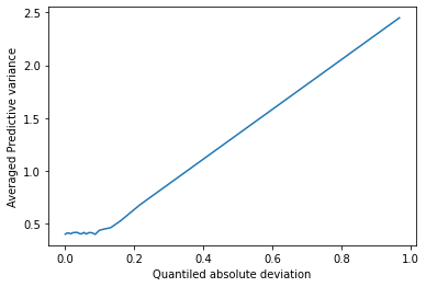
(a) Sim-Poisson Dataset

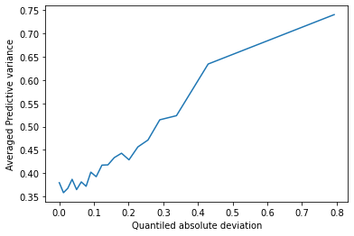
(b) Crime Dataset

Figure 2: Predictive variance against quantiles of absolute deviation.

Dataset	Sim-Poisson	Sim-Hawkes	Music	Crime
correlation	0.537	0.324	0.336	0.107

Table 4: Spearman Coefficient between MAE and PIL (positive value indicates positive correlation)

Relevance of Predictive Uncertainty

Evaluating uncertainty for an event data is a difficult task. We expect a model to be more confident for correct predictions and should exhibit smaller uncertainty. Consequently, it should assign lower PIL for correct predictions and vice-versa. To acknowledge this behavior, we plot Quantile Plots of absolute deviation against the average variance predicted by the model. For this, we consider quantile $q$ of the absolute deviation (AD) of predicted time and actual time $|\hat{t}_{i}-t_{i}|$. Then we average prediction interval length (Avg-PIL), of all the events with absolute deviation less than the quantile value.

$$\text{Avg-PIL}=\{\text{Average}(2*\sigma_{i})|\quad\forall|t_{i}-\hat{t}_{i}|<=\text{q-th quantile}\}$$

We can observe the quantile plots of averaged predictive variance against the absolute deviation of the predicted time for simulated Poisson and Crime dataset in the Figure 2. An increasing line suggests that as absolute deviation increases, predictive uncertainty also increases, hence supporting our hypotheses. We also validate our hypothesis using correlation between predictive variance and AD. We calculate Spearman coefficient between AD and PIL for all the datasets and report in Table 4. Here, we can observe that the Spearman coefficient is positive for all datasets, supporting our hypothesis.

Figure 3: Correlation between MAE and PIL

(a) PIL

(b) MAE

Also, Figure 3 displays averaged AD and PIC for a batch of three for a sequence of events corresponding to a user of Music dataset. Here also, it is evident that the correlation between AD and prediction interval length.

Sensitivity Analysis

We also perform sensitivity analysis on crime dataset for different dropouts. The results are reported in Table 5. We observe that smaller values of dropout probabilities will not change the results much. Though we can obtain a very high PIC value of 0.999 with a drop probability of $0.8$, this is not the best setting due to very high MAE. So, the algorithm is producing wider intervals to cover many events, however the MAE is increasing. On the contrary, dropout 0.1 is producing low MAE, however PIC is also low. So, actual event coverage will be low for such a model.

Spatial Analysis

The proposed approach outputs spatial uncertainty in terms of lower and upper bound on latitude and longitude. To analyze spatial uncertainty in the units of distance, we calculate the distance between the predicted latitude-longitude bounds (PIL) for locations associated with a user from the Foursquare dataset and plot in Figure 4. Also, Table 6 lists the correlation between predictive variance and absolute deviation (AD) for predicted time, latitude and longitude. The positive correlation coefficient indicates that predictive uncertainty increases with increase in AD.

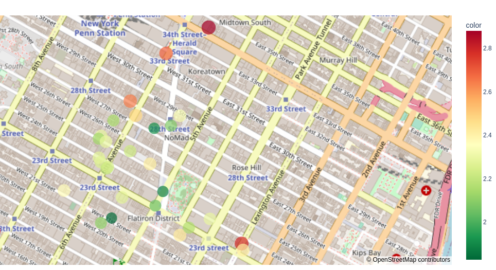
Figure 4: Plots for locations from Foursquare with color coding showing distance between predicted lower and upper bound(in km)

5 Conclusion

We propose Bayesian Neural Hawkes Process for predicting event occurrence times and modelling uncertainty. BNHP combines the advantages of NHP and Bayesian learning, resulting in improved predictive performance and uncertainty modelling capability. The proposed model uses a practical approach based on MC Dropout and extends it for the NHP model. We further develop BNHP for modelling spatio-temporal data. Our experiments on simulated and real datasets demonstrate the efficacy of the proposed approach.

Dropout	MAE	PIC
0.01	0.201	0.294
0.1	0.193	0.227
0.6	0.203	0.737
0.8	5.57	0.999

Table 5: Sensitivity Analysis for
different dropouts for Crime dataset

	Foursq	Taxi
Time	0.91	0.75
Lat	0.17	0.01
Long	0.18	0.01

Table 6: Correlation between MAE and PIL for spatial coordinates.

References

- Abadi et al. [2015] Martín Abadi, Ashish Agarwal, Paul Barham, Eugene Brevdo, Zhifeng Chen, Craig Citro, Greg S. Corrado, Andy Davis, Jeffrey Dean, Matthieu Devin, Sanjay Ghemawat, Ian Goodfellow, Andrew Harp, Geoffrey Irving, Michael Isard, Yangqing Jia, Rafal Jozefowicz, Lukasz Kaiser, Manjunath Kudlur, Josh Levenberg, Dandelion Mané, Rajat Monga, Sherry Moore, Derek Murray, Chris Olah, Mike Schuster, Jonathon Shlens, Benoit Steiner, Ilya Sutskever, Kunal Talwar, Paul Tucker, Vincent Vanhoucke, Vijay Vasudevan, Fernanda Viégas, Oriol Vinyals, Pete Warden, Martin Wattenberg, Martin Wicke, Yuan Yu, and Xiaoqiang Zheng. TensorFlow: Large-scale machine learning on heterogeneous systems, 2015. Software available from tensorflow.org.
- Bacry et al. [2015] Emmanuel Bacry, Iacopo Mastromatteo, and Jean-François Muzy. Hawkes processes in finance. Market Microstructure and Liquidity, 1(01):1550005, 2015.
- Blei et al. [2017] David M. Blei, Alp Kucukelbir, and Jon D. McAuliffe. Variational inference: A review for statisticians. Journal of the American Statistical Association, 112(518):859–877, 2017.
- Chapfuwa et al. [2020] Paidamoyo Chapfuwa, Chenyang Tao, Chunyuan Li, Irfan Khan, Karen J Chandross, Michael J Pencina, Lawrence Carin, and Ricardo Henao. Calibration and uncertainty in neural time-to-event modeling. IEEE Transactions on Neural Networks and Learning Systems, 2020.
- Chen et al. [2020] Ricky TQ Chen, Brandon Amos, and Maximilian Nickel. Neural spatio-temporal point processes. In International Conference on Learning Representations, 2020.
- Chiang et al. [2021] Wen-Hao Chiang, Xueying Liu, and George Mohler. Hawkes process modeling of covid-19 with mobility leading indicators and spatial covariates. International journal of forecasting, 2021.
- Chilinski and Silva [2020] Pawel Chilinski and Ricardo Silva. Neural likelihoods via cumulative distribution functions. In Conference on Uncertainty in Artificial Intelligence, pages 420–429. PMLR, 2020.
- Diggle et al. [2005] Peter Diggle, Barry Rowlingson, and Ting-li Su. Point process methodology for on-line spatio-temporal disease surveillance. Environmetrics: The official journal of the International Environmetrics Society, 16(5):423–434, 2005.
- Du et al. [2016] Nan Du, Hanjun Dai, Rakshit Trivedi, Utkarsh Upadhyay, Manuel Gomez-Rodriguez, and Le Song. Recurrent marked temporal point processes: Embedding event history to vector. In Proceedings of the 22nd ACM SIGKDD International Conference on Knowledge Discovery and Data Mining, pages 1555–1564, 2016.
- Embrechts et al. [2011] Paul Embrechts, Thomas Liniger, and Lu Lin. Multivariate hawkes processes: an application to financial data. Journal of Applied Probability, 48(A):367–378, 2011.
- Gal and Ghahramani [2016a] Yarin Gal and Zoubin Ghahramani. Dropout as a bayesian approximation: Representing model uncertainty in deep learning. In international conference on machine learning, pages 1050–1059. PMLR, 2016.
- Gal and Ghahramani [2016b] Yarin Gal and Zoubin Ghahramani. A theoretically grounded application of dropout in recurrent neural networks. Advances in neural information processing systems, 29:1019–1027, 2016.
- Gal [2016] Yarin Gal. Uncertainty in deep learning. PhD thesis, PhD thesis, University of Cambridge, 2016.
- Graves [2011] Alex Graves. Practical variational inference for neural networks. In Advances in neural information processing systems, pages 2348–2356. Citeseer, 2011.
- Hainzl et al. [2010] Sebastian Hainzl, D Steacy, and S Marsan. Seismicity models based on coulomb stress calculations. Community Online Resource for Statistical Seismicity Analysis, 2010.
- Hawkes [1971] Alan G Hawkes. Spectra of some self-exciting and mutually exciting point processes. Biometrika, 58(1):83–90, 1971.
- Ilhan and Kozat [2020] Fatih Ilhan and Suleyman S Kozat. Modeling of spatio-temporal hawkes processes with randomized kernels. IEEE Transactions on Signal Processing, 68:4946–4958, 2020.
- Lakshminarayanan et al. [2017] Balaji Lakshminarayanan, Alexander Pritzel, and Charles Blundell. Simple and scalable predictive uncertainty estimation using deep ensembles. Advances in Neural Information Processing Systems, 30, 2017.
- Mei and Eisner [2017] Hongyuan Mei and Jason M Eisner. The neural hawkes process: A neurally self-modulating multivariate point process. Advances in Neural Information Processing Systems, 30, 2017.
- Mohler et al. [2011] George O Mohler, Martin B Short, P Jeffrey Brantingham, Frederic Paik Schoenberg, and George E Tita. Self-exciting point process modeling of crime. Journal of the American Statistical Association, 106(493):100–108, 2011.
- Neal [2012] Radford M Neal. Bayesian learning for neural networks, volume 118. Springer Science & Business Media, 2012.
- Okawa et al. [2019] Maya Okawa, Tomoharu Iwata, Takeshi Kurashima, Yusuke Tanaka, Hiroyuki Toda, and Naonori Ueda. Deep mixture point processes: Spatio-temporal event prediction with rich contextual information. In Proceedings of the 25th ACM SIGKDD International Conference on Knowledge Discovery & Data Mining, pages 373–383, 2019.
- Omi et al. [2019] Takahiro Omi, Kazuyuki Aihara, et al. Fully neural network based model for general temporal point processes. Advances in Neural Information Processing Systems, 32:2122–2132, 2019.
- Pearce et al. [2018] Tim Pearce, Alexandra Brintrup, Mohamed Zaki, and Andy Neely. High-quality prediction intervals for deep learning: A distribution-free, ensembled approach. In International Conference on Machine Learning, pages 4075–4084. PMLR, 2018.
- Srivastava et al. [2014] Nitish Srivastava, Geoffrey Hinton, Alex Krizhevsky, Ilya Sutskever, and Ruslan Salakhutdinov. Dropout: a simple way to prevent neural networks from overfitting. The journal of machine learning research, 15(1):1929–1958, 2014.
- Valkeila [2008] Esko Valkeila. An introduction to the theory of point processes, volume ii: General theory and structure, by daryl j. daley, david vere-jones, 2008.
- Wang et al. [2020] Haoyun Wang, Liyan Xie, Alex Cuozzo, Simon Mak, and Yao Xie. Uncertainty quantification for inferring hawkes networks. Advances in Neural Information Processing Systems, 33, 2020.
- Xiao et al. [2017] Shuai Xiao, Junchi Yan, Xiaokang Yang, Hongyuan Zha, and Stephen Chu. Modeling the intensity function of point process via recurrent neural networks. In Proceedings of the AAAI Conference on Artificial Intelligence, volume 31, 2017.
- Xu et al. [2018] Hongteng Xu, Dixin Luo, Xu Chen, and Lawrence Carin. Benefits from superposed hawkes processes. In International Conference on Artificial Intelligence and Statistics, pages 623–631. PMLR, 2018.
- Zhang et al. [2019] R Zhang, C Walder, MA Rizoiu, and L Xie. Efficient non-parametric bayesian hawkes processes. In IJCAI International Joint Conference on Artificial Intelligence, 2019.
- Zhang et al. [2020] Rui Zhang, Christian Walder, and Marian-Andrei Rizoiu. Variational inference for sparse gaussian process modulated hawkes process. In Proceedings of the AAAI Conference on Artificial Intelligence, volume 34, pages 6803–6810, 2020.
- Zhou et al. [2021] Zihao Zhou, Xingyi Yang, Ryan Rossi, Handong Zhao, and Rose Yu. Neural point process for learning spatiotemporal event dynamics. arXiv preprint arXiv:2112.06351, 2021.
- Zuo et al. [2020] Simiao Zuo, Haoming Jiang, Zichong Li, Tuo Zhao, and Hongyuan Zha. Transformer hawkes process. In International Conference on Machine Learning, pages 11692–11702. PMLR, 2020.