2Collège de Bois-de-Boulogne, Montréal, QC, Canada
3Département de Physique, Université de Montréal, Montréal, QC, Canada
11email: m.talafha@astro.elte.hu
Role of observable nonlinearities in solar cycle modulation
Abstract
Context. Two candidate mechanisms have recently been considered with regard to the nonlinear modulation of solar cycle amplitudes. Tilt quenching (TQ) comprises the negative feedback between the cycle amplitude and the mean tilt angle of bipolar active regions relative to the azimuthal direction. Latitude quenching (LQ) consists of a positive correlation between the cycle amplitude and average emergence latitude of active regions.
Aims. Here, we explore the relative importance and the determining factors behind the LQ and TQ effects.
Methods. We systematically probed the degree of nonlinearity induced by TQ and LQ, as well as a combination of both using a grid based on surface flux transport (SFT) models. The roles played by TQ and LQ are also explored in the successful 2x2D dynamo model, which has been optimized to reproduce the statistical behaviour of real solar cycles.
Results. The relative importance of LQ versus TQ is found to correlate with the ratio in the SFT model grid, where is the meridional flow amplitude and is the diffusivity. An analytical interpretation of this result is given, further demonstrating that the main underlying parameter is the dynamo effectivity range, , which is, in turn, determined by the ratio of equatorial flow divergence to diffusivity. The relative importance of LQ versus TQ is shown to scale as . The presence of a latitude quenching effect is seen in the 2x2D dynamo, contributing to the nonlinear modulation by an amount that is comparable to TQ. For other dynamo and SFT models considered in the literature, the contribution of LQ to the modulation covers a broad range – from entirely insignificant to serving as a dominant source of feedback. On the other hand, the contribution of a TQ effect (with the usually assumed amplitude) is never shown to be negligible.
Key Words.:
Sun – Dynamo – Magnetic field – Solar Cycle1 Introduction
The origin of intercycle variations in the series of 11-year solar activity cycles and the possibilities to predict them have been the focus of intense research over the past decade (Petrovay 2020, Charbonneau 2020, Nandy 2021). In a physical system displaying periodic or quasiperiodic behaviour, intercycle variations must be due to either inherent nonlinearities or external forcing. A plausible example is the way in which the strictly sinusoidal, periodic solutions of the simple linear oscillator equation turn into less regular quasiperiodic variations when nonlinear or stochastic forcing terms are added. Indeed, under some simplifying assumptions, the equations describing a solar flux transport dynamo can be truncated to a nonlinear oscillator equation (Lopes et al. 2014).
Here, ”external” forcing refers to the physical model under consideration and not necessarily to the object of study, namely: in mean-field models of the solar dynamo, stochastic variation triggered by small-scale disturbances that are not explicitly modelled is the most plausible source of such forcing. Possibilities for making solar cycle predictions are determined by the nature and interplay of these nonlinear and stochastic effects.
Based on its observed characteristics, the solar dynamo is likely to be an -dynamo, wherein strong toroidal magnetic fields are generated by the windup of a weaker poloidal (north–south) field by differential rotation. The strong toroidal field buried below the surface then occasionally and locally emerges to the surface and protrudes into the atmosphere in the form of east–west oriented magnetic flux loops that are observed as solar active regions. Besides their dominant azimuthal magnetic field component, these loops, presumably under the action of Coriolis force, also develop a poloidal field component which is typically oriented opposite to the preexisting global poloidal field. The evolution of the poloidal magnetic field on the solar surface (where it is effectively radial) can be followed on solar full-disk magnetograms and found to be well described by phenomenological surface flux transport (SFT) models (Jiang et al. 2014). In such SFT models, the evolution of the radial magnetic field at the surface is described by an advective-diffusive transport equation, with an added source term representing emerging active regions and an optional sink term to describe the effects of radial diffusion. Advection is attributed to the poleward meridional flow, while diffusion is due to supergranular motions.
At solar minimum, the field is found to be strongly concentrated at the Sun’s poles, so the dominant contribution to the solar dipole moment, namely:
| (1) |
(where : latitude, : time, : azimuthally averaged field strength) comes from the polar caps. It is this polar field that serves as seed for the windup into the toroidal field of the next solar cycle, so for intercycle variations it is sufficient to consider the azimuthally averaged SFT equation. This is expressed as:
| (2) | |||||
where is the solar radius, is the supergranular diffusivity, is the meridional flow speed, is the time scale of decay due to radial diffusion, and is the source representing flux emergence.
As Eq. (2) is linear, the amplitude of the dipole moment, , built up by the end of cycle is uniquely set by the inhomogeneous term, . The windup of the poloidal field, , in turn, is expected to be linearly related to the peak amplitude of the toroidal field in cycle, , and, hence, to the amplitude of the next activity cycle — this is indeed confirmed by both observations and dynamo models (Muñoz-Jaramillo et al. 2013, Kumar et al. 2021). The only step where nonlinearities and stochastic noise can enter this process is thus via flux emergence, linking the subsurface toroidal field to the poloidal source at the surface. As is directly accessible to observations, this implies that the nonlinearities involved may, in principle, be empirically constrained.
Indeed, Dasi-Espuig et al. (2010) reported that the average tilt of the axis of bipolar active regions relative to the azimuthal direction is anticorrelated with regard to the cycle amplitude. Starting with the pioneering work of Cameron et al. (2010), this tilt quenching (TQ) effect has become widely used in solar dynamo modeling, especially as the product of the mean tilt with the cycle amplitude has been shown to be a good predictor of the amplitude of the next cycle. The observational evidence, however, is still inconclusive, and the numerical form of the effect remains insufficiently constrained (see, however, Jiao et al. 2021 for more robust recent evidence and also Jha et al. 2020 for the effect’s dependence on field strength).
Jiang (2020) recently called attention to another nonlinear modulation mechanism: latitude quenching (LQ). This is based on the emprirical finding based on an analysis of a long sunspot record, which shows that the mean latitude where active regions emerge in a given phase of the solar cycle is correlated with the cycle amplitude. From higher latitudes, a lower fraction of leading flux can manage become diffused across the equator, leaving less trailing flux to contribute to the polar fields. Therefore, the correlation found here represents a negative feedback effect. Assuming a linear dependence for both the mean tilt and the mean latitude on cycle amplitude, based on one particular SFT setup, Jiang (2020) found that TQ and LQ yield comparable contributions to the overall nonlinearity in the process of the regeneration of the poloidal field from the poloidal source. The net result showed that the net dipole moment change during a cycle tends to be saturated for stronger cycles.
Our objective in the present work is to further explore the respective roles played by TQ and LQ in the solar dynamo. In Section 2, we extend the analysis to other SFT model setups and study how the respective importance of TQ and LQ depend on model parameters. In Section 3, we further consider a case where the form of TQ is explicitly assumed to be nonlinear, namely: the 2x2D dynamo model. Our conclusions are summarized in Section 4.
2 Quadratic nonlinearities in a surface flux transport model
2.1 Model
For the study of how different nonlinearities compare in SFT models with different parameter combinations, our model setup is a generalization of the approach of Petrovay & Talafha (2019) (hereafter Paper 1).
In the prior study, our intention was to model “typical” or “average” solar cycles, so that our source function would not consist of individual ARs but a smooth distribution (interpreted as an ensemble average) representing the probability distribution of the emergence of leading and trailing polarities on the solar surface. By nature, this source is thus axially symmetric, so our whole SFT model is reduced to one dimension, as described by Eq. (2).
For the meridional flow, we consider a sinusoidal profile with a dead zone around the poles,
| (3) |
with . This profile has been used in many other studies, including Jiang (2020), who took the values ms, kms, and .
Our source term is a generalization of the source used in Paper 1. The source is a smooth distribution representing an ensemble average or probability distribution of the emergence of leading and trailing polarities on the solar surface (Cameron & Schüssler 2007, Muñoz-Jaramillo et al. 2010), represented as a pair of rings of opposite magnetic polarities:
| (4) | |||||
where is a factor that depends on the sign of the toroidal field and is the amplitude for cycle . In the numerical implementation of this source profile, care was taken to ensure zero net flux on the spherical surface by reducing the amplitude of the equatorward member of each pair by an appropriate sphericity factor .
is the time profile of activity in a cycle while characterizes the latitude dependence of activity at a given cycle phase. In contrast to Paper 1 where a series of identical cycles was considered, here we allow for intercycle variations, so will be different for each cycle.
The time profile of solar activity in a typical cycle was determined by Hathaway et al. (1994) from the average of many cycles as:
| (5) |
with , , , where is the time since the last cycle minimum.
The latitudinal profile is a Gaussian migrating equatorward during the course of a cycle:
| (6) |
with the constant fixed as . Following the empirical results of Jiang et al. (2011), the standard deviation is given by:
| (7) |
where year is the cycle period. We note that alternate fitting formulae were determined by Lemerle et al. 2015 on the basis of a single cycle.
We obtain the latitudinal separation of the rings as a consequence of Joy’s law, while the mean latitude was again empirically determined by Jiang et al. (2011). These parameters, in turn, are now dependent on cycle amplitude introducing two nonlinearities into the problem.
Tilt Quenching (TQ): Joy’s law varies depending on the amplitude of the cycle as
| (8) |
Here, is an arbitrary reference value corresponding to a “typical” or average cycle amplitude, as set by the nonlinear limitation of the dynamo. Equation (8), thus, measures the departure of the feedback from its value in this reference state; its assumed linear form should be valid for a restricted range in and is not incompatible with the rather lax observational constraints,— cf. Fig. 1b in Jiang (2020). The nonlinearity parameter is another free parameter to be explored; our reference value for it will be 0.15.111We note that alternate functional forms for Joy’s law, admitted by the observational constraints, such as or have also been tested in the context of the linear case (Paper 1) and found to have only a minor impact on the results.
Latitude Quenching (LQ): following Jiang et al. (2011) for the mean latitude of activity at a given phase of cycle we have:
| (9) |
with the mean latitude in cycle given by:
| (10) |
Here, the nonlinearity parameter is fairly tightly constrained by the empirical results of Jiang et al. (2011) as .
For the SFT model parameters, our model grid will be a subset of the grid described in Paper 1. For we only consider two values here: a decay time scale of eight years, comparable to the cycle length and supported by a number of studies (see Paper 1 and references therein), and the reference case with effectively no decay ( years). For m/s, the full set of values in the grid is considered; and similarly for kms, the full set of values is studied (as listed in Table 2). Furthermore, for the study of the effects of individual nonlinearities, for each parameter combination in the SFT model four cases will be considered, as listed in Table 1.
| Case | ||
|---|---|---|
| noQ | 0 | 0 |
| TQ | 0 | 0.15 |
| LQ | 2.4 | 0 |
| LQTQ | 2.4 | 0.15 |
For each combination of the parameters , , , , and we run the SFT code solving Eq. (2) for 1000 solar cycles to produce a statistically meaningful sample of cycles.
2.2 Results
In order to study how the nonlinearities affect the dipole moment built up during cycles of different amplitudes, here we consider the purely stochastic case where individual cycle amplitudes are drawn from a statistical distribution without any regard for previous solar activity. The factor in Eq. (4) is assumed to alternate between even and odd cycles. The form of the statistical distribution chosen is not important for our current purpose but, for concreteness, fluctuations are represented as multiplicative noise applied to the amplitude of the poloidal field source. This noise then follows lognormal statistics: , where is a gaussian random variable of zero mean and standard deviation of . The coefficient for an average cycle is set to to ensure that the resulting dipolar moments roughly agree with observed values (in Gauss).
We note that the latitude-integrated amplitude of our source term must be linearly related to the observed value of the smoothed international sunspot number:
The proportionality coefficient, was arbitrarily tuned to closely reproduce the observed mean value of for each value of .
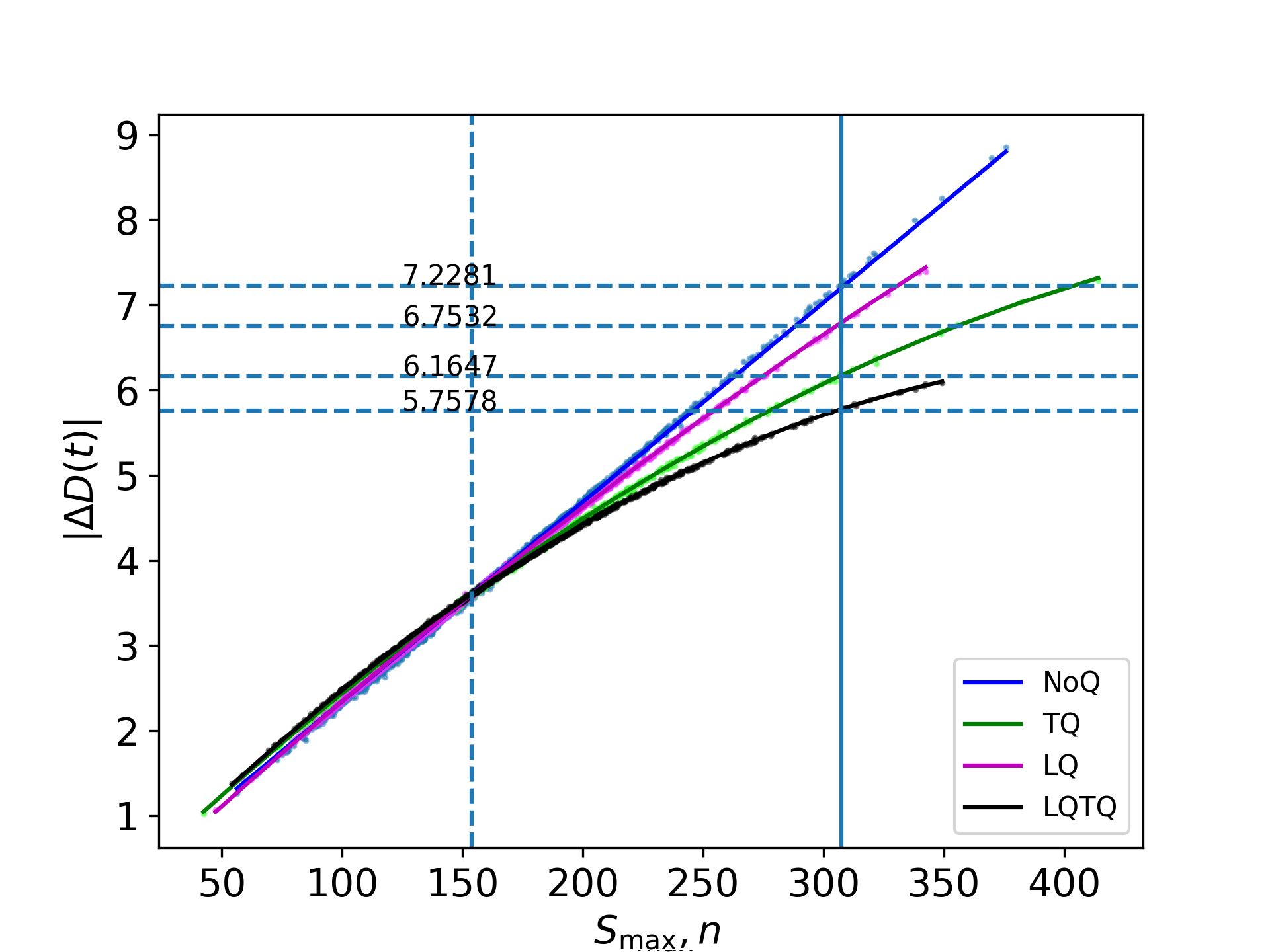
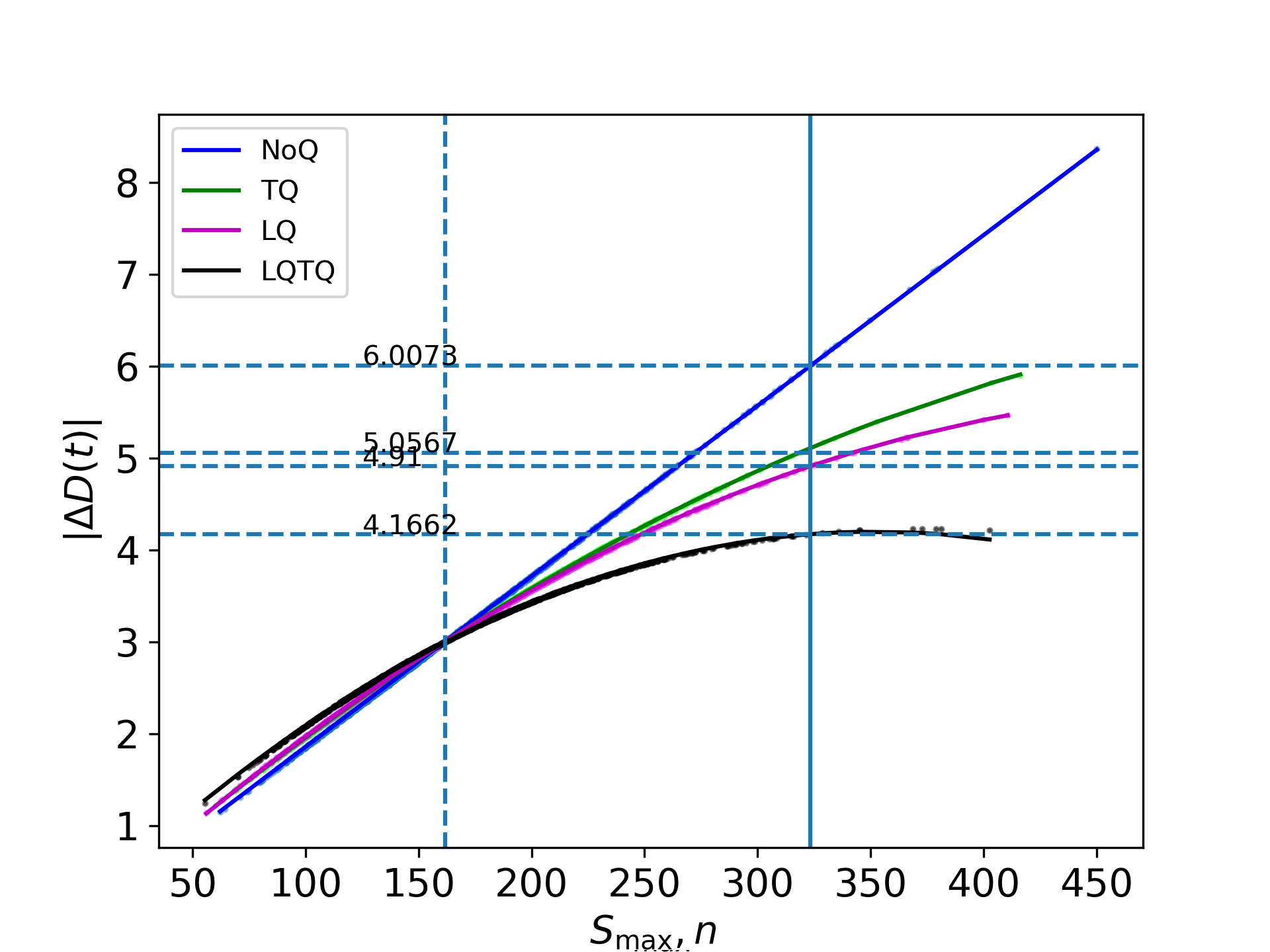
Introducing the notation (with in years), the net contribution of cycle to the change in dipolar moment is given by . Figures 1 and 2 display against the cycle amplitude for some example runs.
The linear case (noQ) is obviously well suited to a linear fit, while all three nonlinear cases are seen to be well represented by quadratic fits forced to intersect the linear fit at the mean value of .
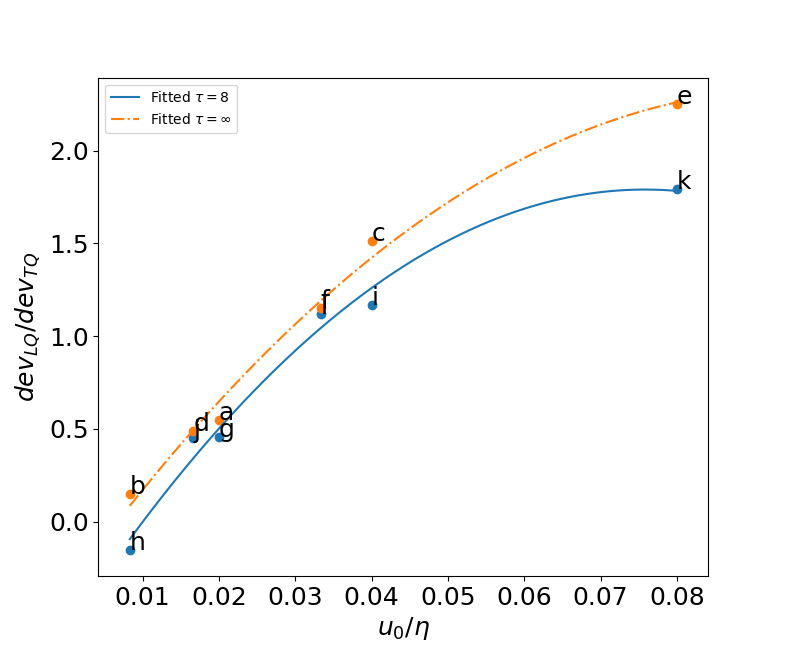
The respective importance of TQ and LQ is seen to differ for these cases. For a quantitative characterization of the influence of nonlinearities we use the deviation of from the linear case at an arbitrary selected value of (roughly twice the mean), as illustrated by the solid vertical lines in Figs. 1–2. To give an example, in the TQ case, the deviation is for the model in Fig. 1. The relative importance of latitude quenching versus tilt quenching is then characterized by the ratio of these deviations for the LQ and TQ cases, . Comparing these values to several parameter combinations reveals that the relative importance of the two effects is primarily determined by the ratio . This is borne out in Fig. 3.
| case | [yr] | [ms] | [kms] | [∘] |
|---|---|---|---|---|
| a | 5 | 250 | 12.35 | |
| b | 5 | 600 | 18.52 | |
| c | 10 | 250 | 9.44 | |
| d | 10 | 600 | 13.41 | |
| e | 20 | 250 | 7.79 | |
| f | 20 | 600 | 10.05 | |
| g | 8 | 5 | 250 | 12.35 |
| h | 8 | 5 | 600 | 18.52 |
| i | 8 | 10 | 250 | 9.44 |
| j | 8 | 10 | 600 | 13.41 |
| k | 8 | 20 | 250 | 7.79 |
| l | 8 | 20 | 600 | 10.05 |
2.3 Interpretation
Over a short interval of time the smooth source distribution assumed, Eq. (4) is reduced to a bipole with a flux of
| (11) | |||||
in each polarity.
The ultimate contribution of such a bipole to the solar axial dipole moment after several years has been analytically derived by Petrovay et al. (2020) as:
| (12) |
where is the initial contribution of the bipole to the global dipole moment, is the time of the minimum of the next cycle, while the asymptotic dipole contribution factor is given by:
| (13) |
Here, is a constant and defining as the divergence of the meridional flow at the equator and the dynamo effectivity range is a universal function of for plausible choices of the meridional flow profile.
For the source considered here:
| (14) |
Combining the last three equations and integrating for the full duration of the cycle yields the net change in the solar dipole moment:
| (15) |
with
| (16) |
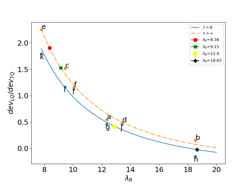
This shows that and, hence, the nonlinear effects in it, only depend on model parameters through and the dynamo effectivity range . For a fixed meridional flow profile, as used in this work, , hence is uniquely related to , explaining the dependence on the latter variable, as shown in Fig. 3. On the other hand, usinq Eqs. (26) and (27) of Petrovay et al. (2020), can be derived for each of our models, allowing us to plot the underlying relation of the nonlinearity ratios with . This plot is displayed in Fig. 4.
In order to understand the form of this relation we recall from Eqs. (8)–(10) that
| (17) |
Upon substituting the Eqs. (8)–(10) into (15), the deviations from the linear case correspond to the terms containing and . We will consider these terms in the limit and, relying on the mean value theorem for integrals, time integrals will be substituted by the product of the cycle period and the value of the integrand for an appropriately defined average. These weighted averages are not expected to differ from the unweighted average by more than a few degrees, so they will be substituted here simply by for an approximation.
In the TQ case, using Eq. (8), the term containing is immediately found to scale as
| (18) |
The LQ case is slightly more complex. In the limit , the dependence on the latitude of activity enters Eq. (15) through the combination . A Taylor expansion yields:
| (19) |
Substituting here and plugging the expression back into Eq. (15), the term involving is found to scale as:
| (20) |
2.4 Discussion
It is to be noted in Fig. 4 that for high
values of , the value of becomes slightly negative.
This is due to the circumstance that latitudinal quenching can affect
in two ways:
(i) by modulating the fraction of active regions above
that do not contribute to , which results in a negative
feedback; (ii) by modulating the mean tilt angle of active regions in accordance
with Joy’s law, which is a positive feedback effect.
For the first effect dominates. However, when significantly exceeds the fraction of ARs above becomes negligible, so only the second, positive feedback effect remains. As a result, changes sign.
A slight dependence on is also noticed. This can be attributed to the fact that for shorter values of the dipole moment contribution of ARs appearing early in the cycle will have more time to decay until the next minimum, hence, these ARs will have a lower relative contribution to . But the ARs in the early part of the cycle are the ones at the highest latitudes, that is, they are most affected by LQ via effect (i) above. Hence, for shorter values of the relative importance of LQ is expected to be slightly suppressed. This suppression may be expected to vanish towards higher values of , in agreement with Fig. 4.
The larger, coloured symbols in Fig. 4 mark the positions of various dynamo and SFT models discussed in recent publications. It is apparent that the case where LQ results in a positive feedback is not strictly of academic interest: at least one SFT model discussed recently, namely, that of Whitbread et al. (2018) is in this parameter range. The parameter choice for this model was motivated by an overall optimization of observed versus simulated magnetic supersynoptic maps (Whitbread et al. 2017). At the other end of the scale, the low diffusivity, medium flow speed models of Bhowmik & Nandy (2018) and Jiang & Cao (2018) are in a range where LQ is manifest as a negative feedback giving the dominating contribution to the nonlinearity, although the effect of TQ remains non-negligible.
Conversely, the locus of the SFT component of the 2x2D model of Lemerle & Charbonneau (2017) in Fig. 4 indicates that if the TQ and LQ effects were formulated as in our model, the contributions of TQ should dominate but the negative feedback due to LQ would also contribute quite significantly to the nonlinearity. We take a closer look at this model in the following section.
As a caveat regarding the validity of these conclusions, we recall that the results presented in this section are based on the assumption of one particular form of the time profile of the source function, Eq. (5), with constant parameters and a strictly fixed periodicity of 11 years. As long as deviations from it are stochastic, this source may still be considered representative as an ensemble average. However, there have also been indications of systematic deviations.
It is well known that the length of solar cycles is inversely related to their amplitude: this effect implies an inverse correlation of the parameter in Eq. (5) with (or, equivalently, ). It is, however, straightforward to see that a variation in will not affect our results. If is kept constant, as suggested by Hathaway et al. (1994), is the only time scale appearing in , so, with fixed, its variation will simply manifest as a self-similar temporal expansion or contraction of the profile (5). As a result, cycle lengths will then vary and so will the area below the curve, namely, the total amount of emerging flux, and, hence, the amplitude of the dipole moment source. As a result, the dipole moment built up by the end of the cycle will linearly scale with . This scaling factor, however, will be the same for the TQ, LQ, and subsequent cases, so the ratio between their deviations, plotted in Figure 4, remains unaffected.
Furthermore, Jiang et al. (2018) noted that actual cycle profiles tend to show a systematic upward deviation from the profile (5) in their late phases. Such an effect would indeed had an impact on our results somewhat. As in these late phases the activity is concentrated near the equator, at latitudes well below , the extra contribution to the dipole moment due to this excess is not expected to be subject to LQ, while it is still affected by TQ. Hence, , plotted in Figure 4, is expected to be somewhat lower with this correction. This relative difference, in turn, may be expected to vanish towards higher values of , where LQ becomes insignificant anyway.
3 Nonlinear effects in the 2x2D dynamo model
In this section, we consider the role of nonlinearities in a full dynamo model, namely, the 2x2D dynamo model (Lemerle et al. 2015 and Lemerle & Charbonneau 2017). This model, also used for solar cycle forecast (Labonville et al. 2019), couples a 2D surface SFT model with an axisymmetric model of the dynamo operating in the convective zone. The azimuthal average of the poloidal magnetic field resulting from the SFT component is used as upper boundary condition in the subsurface component, while the source term in the SFT model is a set of bipolar magnetic regions (BMRs) introduced instantaneously with a probability related to the amount of toroidal flux in a layer near the base of the convective zone, as a simplified representation of the flux emergence process. The model has a large number of parameters optimized for best reproduction of the observed characteristics of solar cycle 21.
3.1 Nonlinearity vs. stochastic scatter in the 2x2D dynamo
Figure 5 presents the equivalent of Figs. 1 and 2 for 5091 cycles simulated in the 2x2D model. A marked nonlinearity is clearly seen: the net contribution of a cycle to the dipole moment increases slower than in the linear case with cycle amplitude, representing a negative feedback, similarly to the case of the pure SFT model.
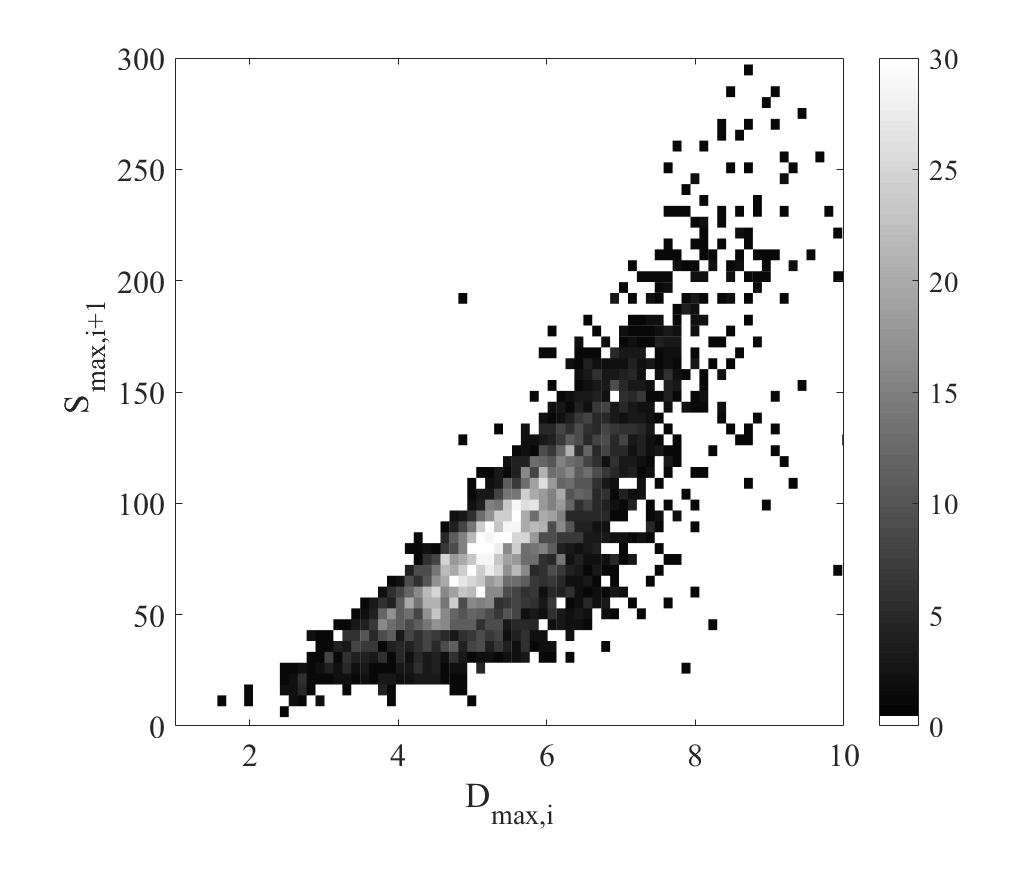
In the dynamo model, the dipole moment built up during a cycle feeds back into the cycle as the amplitude of the toroidal field generated by the windup of the poloidal fields (and, hence, the amplitude of the upcoming cycle) increases with the amplitude of the poloidal field. This is borne out in Fig. 6. We note that the relation is not exactly linear and there is a slight threshold effect at work, which is presumably related to the requirement that the toroidal field must exceed a minimal field strength for emergence.
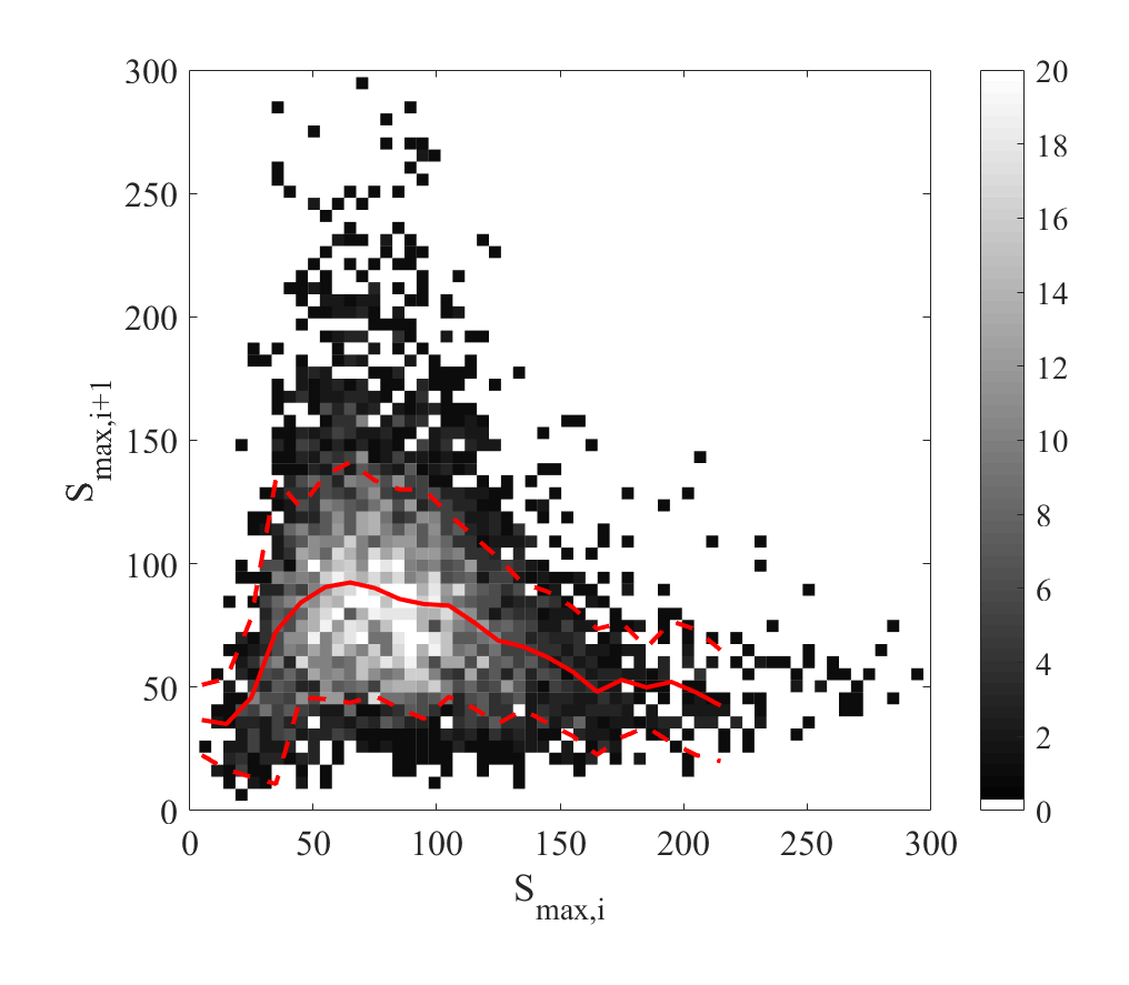
The combined result of the two feedbacks presented in Figs. 5 and 6 is a nonlinear coupling between the amplitudes of subsequent cycles as shown in Fig. 7. The convex shape of the median curve implies that on average, very weak cycles will be followed by stronger cycles and very strong cycles will be followed by weak cycles. However, there is a very large amount of scatter present in the plot. A comparison with the scatter in Figs. 5 and 6 shows that the main contribution to the scatter comes from Fig. 5. As is uniquely determined by the source term in the SFT equation representing flux emergence, the main cause of random scatter around the mean nonlinear relation is identified as the stochastic nature of the flux emergence process, namely, the scatter in the time, location, and properties of individual active regions (BMRs in the 2x2D model) statistically following the evolution of the underlying toroidal field.
3.2 Latitude quenching in the 2x2D dynamo model
The question arises as to whether the nonlinearity plotted in Fig. 5 is a consequence of TQ, LQ, or both. Apart from a threshold effect which was not found to be strong or even necessarily needed in the optimized model, the only nonlinearity explicitly built into the 2x2D model is TQ. The tilt angle (i.e., initial dipole contribution ) of a BMR is assumed to scale with
| (22) |
where is the quenching field amplitude.
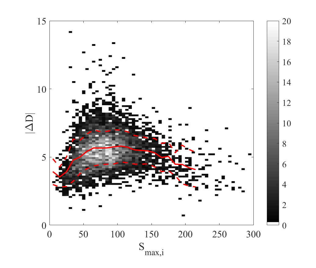
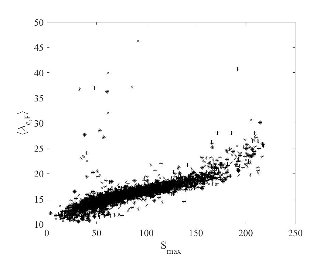
As the latitudinal distribution of BMRs is fed into the SFT component of the 2x2D model from the mean-field component, LQ cannot be imposed. Nevertheless, this does not mean that LQ is not present. Indeed, as demonstrated in Fig. 8, the 2x2D model displays a very marked latitude quenching effect, with a tight correlation between the mean emergence latitude of BMRs and cycle amplitude. This LQ is even stronger than witnessed in the Sun, varying by as varies between and . In contrast, according to Eq. (10), only varies by about (from to ) for the same range in .
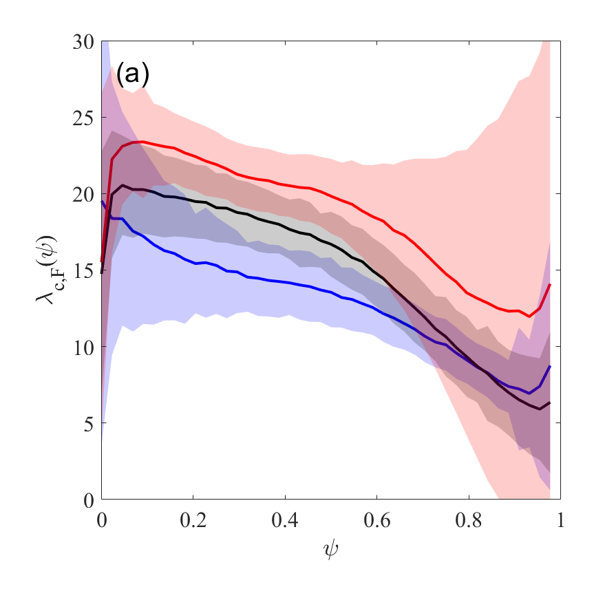
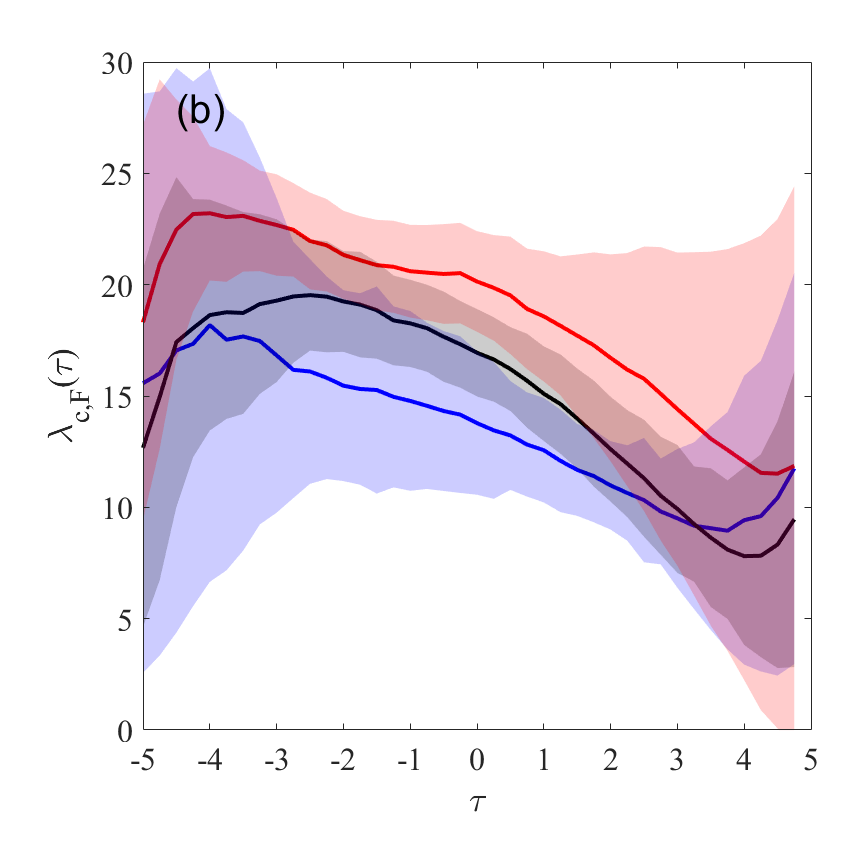
The origin of this LQ effect is elucidated in Fig. 9. Three subsamples of all simulated cycles are considered: cycles stronger or weaker than the mean amplitude by at least 1 standard deviation are displayed in red or blue, respectively, while black marks cycles not farther from the mean amplitude than 0.1 standard deviation. The plots clearly demonstrate that tracks of latitudinal migration of these three subsets are systematically shifted relative to each other. The alternative possibility that all cycles follow the same track with LQ resulting from the different temporal variation of the activity level can thus be discarded.
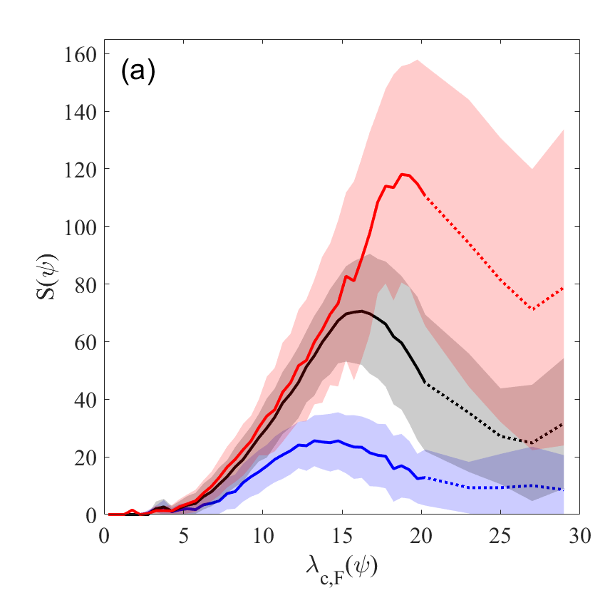
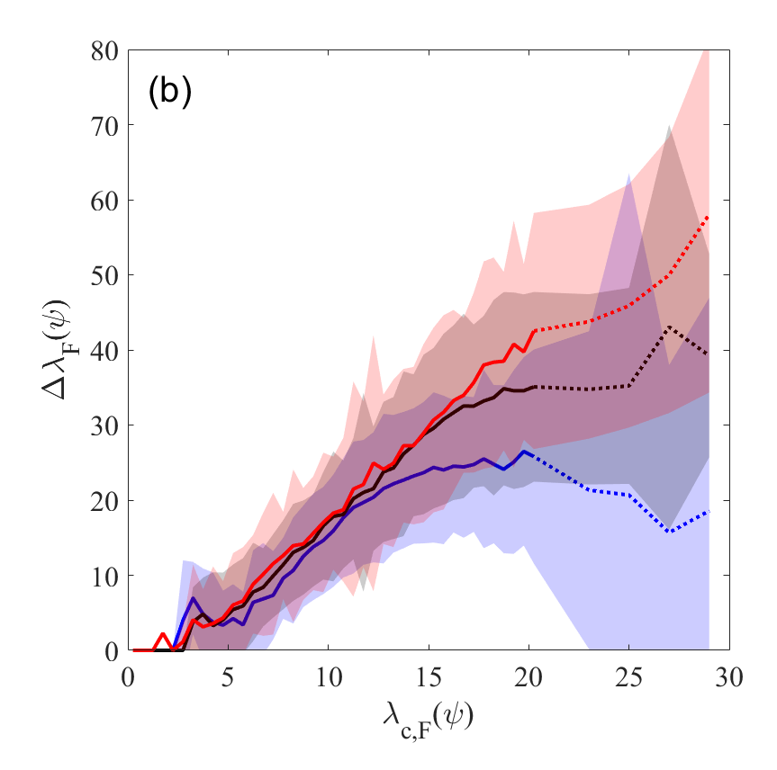
Cameron & Schüssler (2016) considered the time evolution of mean latitude and width of the activity belts in observed solar cycles, interpreting the decay phase of cycles as a result of the cancellation of oppositely oriented toroidal flux bundles across the equator by turbulent diffusion. They pointed out that this leads to a certain universality of the characteristics of the decay phases in different solar cycles. Our finding that the tracks of migrating toroidal flux bundles systematically differ for strong and weak cycles may at first sight seem to contradict this interpretation. However, a closer look at the properties of decay phases of cycles simulated in the 2x2D model confirms the universality posited by Cameron & Schüssler (2016). In Fig. 10a, we present the evolution of the (pseudo) sunspot number simulated in the models against the latitude of activity belts, rather than against time, while Fig. 10b presents the evolution of the width of the latitudinal distribution of BMRs in a similar way (see Figs. 3 and 4 in Cameron & Schüssler 2016 for the observational equivalents of these plots.) It is apparent that the curves for the strong, average and weak subsamples are nicely aligned towards their low-latitude (i.e., late-phase) ends, confirming the universality proposition.
4 Conclusion
In this work, we explore the relative importance and the determining factors behind the LQ and TQ effects. The degree of nonlinearity induced by TQ, LQ, and their combination was systematically probed in a grid of surface flux transport (SFT) models. The relative importance of LQ versus TQ has been found to correlate with the ratio in the SFT model grid, where is the meridional flow amplitude and is diffusivity. An analytical interpretation of this result has been given, further showing that the main underlying parameter is the dynamo effectivity range , which, in turn, is determined by the ratio of equatorial flow divergence to diffusivity. The relative importance of LQ versus TQ was found to scale as .
As displayed in Fig. 4, for various dynamo and SFT models considered in the literature the contribution of LQ to the amplitude modulation covers a broad range from being insignificant to being the dominant form of feedback. On the other hand, the contribution of a TQ effect (with the usually assumed amplitude) is never negligible.
The role of TQ and LQ was also explored in the 2x2D dynamo model optimized to reproduce the statistical behaviour of real solar cycles. We demonstrated the presence of latitude quenching in the 2x2D dynamo. The locus of the SFT component of the model in Fig. 4 suggests that LQ contributes to the nonlinear modulation by an amount comparable to TQ. This LQ effect is present in the model despite the lack of any modulation in the meridional flow. We note that the meridional inflow module of the 2x2D model developed by Nagy et al. 2020 was not used for these runs. This agrees with the results of Karak (2020) who showed the presence of latitude quenching in the STABLE dynamo model with a steady meridional flow. As LQ is rather well constrained on the observational side (Jiang 2020), its presence and character may potentially be used in the future as a test or merit function in the process of fine-tuning of dynamo models to solar observations.
Acknowledgements.
This research was supported by the Hungarian National Research, Development and Innovation Fund (grants no. NKFI K-128384 and TKP2021-NKTA-64), by the European Union’s Horizon 2020 research and innovation programme under grant agreement No. 955620, and by the Fonds de Recherche du Québec – Nature et Technologie (Programme de recherche collégiale). The collaboration of the authors was facilitated by support from the International Space Science Institute in ISSI Team 474.References
- Bhowmik & Nandy (2018) Bhowmik, P. & Nandy, D. 2018, Nature Communications, 9, 5209
- Cameron & Schüssler (2007) Cameron, R. & Schüssler, M. 2007, ApJ, 659, 801
- Cameron et al. (2010) Cameron, R. H., Jiang, J., Schmitt, D., & Schüssler, M. 2010, ApJ, 719, 264
- Cameron & Schüssler (2016) Cameron, R. H. & Schüssler, M. 2016, A&A, 591, A46
- Charbonneau (2020) Charbonneau, P. 2020, Living Reviews in Solar Physics, 17, 4
- Dasi-Espuig et al. (2010) Dasi-Espuig, M., Solanki, S. K., Krivova, N. A., Cameron, R., & Peñuela, T. 2010, A&A, 518, A7
- Hathaway et al. (1994) Hathaway, D. H., Wilson, R. M., & Reichmann, E. J. 1994, Solar Physics, 151, 177
- Jha et al. (2020) Jha, B. K., Karak, B. B., Mandal, S., & Banerjee, D. 2020, ApJ, 889, L19
- Jiang (2020) Jiang, J. 2020, ApJ, 900, 19
- Jiang et al. (2011) Jiang, J., Cameron, R. H., Schmitt, D., & Schüssler, M. 2011, A&A, 528, A82
- Jiang & Cao (2018) Jiang, J. & Cao, J. 2018, Journal of Atmospheric and Solar-Terrestrial Physics, 176, 34
- Jiang et al. (2014) Jiang, J., Hathaway, D. H., Cameron, R. H., et al. 2014, Space Sci. Rev., 186, 491
- Jiang et al. (2018) Jiang, J., Wang, J.-X., Jiao, Q.-R., & Cao, J.-B. 2018, The Astrophysical Journal, 863, 159
- Jiao et al. (2021) Jiao, Q., Jiang, J., & Wang, Z. 2021, A&A, 653, A27
- Karak (2020) Karak, B. B. 2020, ApJ, 901, L35
- Kumar et al. (2021) Kumar, P., Nagy, M., Lemerle, A., Karak, B. B., & Petrovay, K. 2021, ApJ, 909, 87
- Labonville et al. (2019) Labonville, F., Charbonneau, P., & Lemerle, A. 2019, Sol. Phys., 294, 82
- Lemerle & Charbonneau (2017) Lemerle, A. & Charbonneau, P. 2017, ApJ, 834, 133
- Lemerle et al. (2015) Lemerle, A., Charbonneau, P., & Carignan-Dugas, A. 2015, ApJ, 810, 78
- Lopes et al. (2014) Lopes, I., Passos, D., Nagy, M., & Petrovay, K. 2014, Space Sci. Rev., 186, 535
- Muñoz-Jaramillo et al. (2013) Muñoz-Jaramillo, A., Balmaceda, L. A., & DeLuca, E. E. 2013, Phys. Rev. Lett., 111, 041106
- Muñoz-Jaramillo et al. (2010) Muñoz-Jaramillo, A., Nandy, D., Martens, P. C. H., & Yeates, A. R. 2010, ApJ, 720, L20
- Nagy et al. (2020) Nagy, M., Lemerle, A., & Charbonneau, P. 2020, Journal of Space Weather and Space Climate, 10, 62
- Nandy (2021) Nandy, D. 2021, Sol. Phys., 296, 54
- Petrovay (2020) Petrovay, K. 2020, Living Reviews in Solar Physics, 17, 2
- Petrovay et al. (2020) Petrovay, K., Nagy, M., & Yeates, A. R. 2020, Journal of Space Weather and Space Climate, 10, 50
- Petrovay & Talafha (2019) Petrovay, K. & Talafha, M. 2019, A&A, 632, A87
- Whitbread et al. (2018) Whitbread, T., Yeates, A. R., & Muñoz-Jaramillo, A. 2018, ApJ, 863, 116
- Whitbread et al. (2017) Whitbread, T., Yeates, A. R., Muñoz-Jaramillo, A., & Petrie, G. J. D. 2017, A&A, 607, A76