Differentially-Private Clustering of Easy Instances

Abstract

Clustering is a fundamental problem in data analysis. In differentially private clustering, the goal is to identify $k$ cluster centers without disclosing information on individual data points. Despite significant research progress, the problem had so far resisted practical solutions. In this work we aim at providing simple implementable differentially private clustering algorithms that provide utility when the data is ”easy,” e.g., when there exists a significant separation between the clusters.

We propose a framework that allows us to apply non-private clustering algorithms to the easy instances and privately combine the results. We are able to get improved sample complexity bounds in some cases of Gaussian mixtures and $k$-means. We complement our theoretical analysis with an empirical evaluation on synthetic data.

1 Introduction

Differential privacy [DMNS06] is a mathematical definition of privacy, that aims to enable statistical analyses of databases while providing strong guarantees that individual-level information does not leak. Privacy is achieved in differentially private algorithms through randomization and the introduction of “noise” to obscure the effect of each individual, and thus differentially private algorithms can be less accurate than their non-private analogues. In most cases, this loss in accuracy is studied theoretically, using asymptotic tools. As a result, there is currently a significant gap between what is known to be possible theoretically and what can be done in practice with differential privacy. In this work we take an important step towards bridging this gap in the context of clustering related tasks.

The construction of differentially private clustering algorithms has attracted a lot of attention over the last decade, and many different algorithms have been suggested. However, to the best of our knowledge, none of these algorithms have been implemented: They are not particularly simple and suffer from large hidden constants that translate to a significant loss in utility, compared to non-private implementations.

Question .

How hard is it to cluster privately with a practical implementation?

We take an important step in this direction using the following approach. Instead of directly tackling “standard” clustering tasks, such as $k$-means clustering, we begin by identifying a very simple clustering problem that still seems to capture many of the challenges of practical implementations (we remark that this problem is completely trivial without privacy requirements). We then design effective (private) algorithms for this simple problem. Finally, we reduce “standard” clustering tasks to this simple problem, thereby obtaining private algorithms for other tasks.

In more detail, we introduce the following problem, called the $k$-tuple clustering problem.

Definition (informal, revised in Definition 3).

An instance of the $k$-tuple clustering problem is a collection of $k$-tuples. Assuming that the input tuples can be partitioned into $k$ “obvious clusters”, each consisting of one point of each tuple, then the goal is to report $k$ “cluster-centers” that correctly partition the input tuples into clusters. If this assumption on the input structure does not hold, then the outcome is not restricted.

Remark .

1. By “obvious clusters” we mean clusters which are far away from each other.

2. The input tuples are unordered. This means, e.g., that the “correct” clustering might place the first point of one tuple with the fifth point of another tuple.

3. Of course, we want to solve this problem while guaranteeing differential privacy. Intuitively, this means that the outcome of our algorithm should not be significantly effected when arbitrarily modifying one of the input tuples.

Observe that without the privacy requirement this task is trivial: We can just take one arbitrary input tuple $(x_{1},...,x_{k})$ and report it. With the privacy requirement, this task turns out to be non-trivial. It’s not that this problem cannot be solved with differential privacy. It can. It’s not even that the problem requires large amounts of data asymptotically. It does not. However, it turns out that designing an implementation with a practical privacy-utility tradeoff, that is effective on finite datasets (of reasonable size), is quite challenging.

1.1 Our algorithms for the ${\boldsymbol{k}}$-tuple problem

We present two (differentially private) algorithms for the $k$-tuple clustering problem, which we call $\mathsf{PrivatekAverages}$ and $\mathsf{PrivatekNoisyCenters}$. Both algorithms first privately test if indeed the input is partitioned into $k$ obvious clusters and quit otherwise. They differ by the way they compute the centers in case this test passes. Algorithm $\mathsf{PrivatekAverages}$ privately averages each identified cluster. Algorithm $\mathsf{PrivatekNoisyCenters}$, on the other hand, does not operate by averaging clusters. Instead, it selects one of the input $k$-tuples, and then adds a (relatively small) Gaussian noise to every point in this tuple. We prove that this is private if indeed there are $k$ obvious clusters in the input. We evaluate these two algorithms empirically, and show that, while algorithm $\mathsf{PrivatekAverages}$ is “better in theory”, algorithm $\mathsf{PrivatekNoisyCenters}$ is much more practical for some interesting regimes of parameters.

We now give a simplified overview of the ideas behind our algorithms. For concreteness, we focus here on $\mathsf{PrivatekAverages}$. Recall that in the $k$-tuple clustering problem, we are only required to produce a good output assuming the data is “nice” in the sense that the input tuples can be clustered into $k$ “far clusters” such that every cluster contains exactly one point from every tuple. However, with differential privacy we are “forced” to produce good outputs even when this niceness assumption does not hold. This happens because if the input data is “almost nice” (in the sense that modifying a small number of tuples makes it nice) then differential privacy states that the outcome of the computation should be close to what it is when the input data is nice.

So, the definition of differential privacy forces us to cope with “almost nice” datasets. Therefore, the niceness test that we start with has to be a bit clever and “soft” and succeed with some probability also for data which is “almost nice”. Then, in order to achieve good performances, we have to utilize the assumption that the data is “almost nice” when we compute the private centers. To compute these centers, Algorithm $\mathsf{PrivatekAverages}$ determines (non-privately) a clustering of the input tuples, and then averages (with noise) each of the clusters. The conceptual challenge here is to show that even though the clustering of the data is done non-privately, it is stable enough such that the outcome of this algorithm still preserves privacy.

1.2 Applications

The significance of algorithms $\mathsf{PrivatekAverages}$ and $\mathsf{PrivatekNoisyCenters}$ is that many clustering related tasks can be privately solved by a reduction to the $k$-tuple clustering problem. In this work we explore two important use-cases: (1) Privately approximating the $k$-means under stability assumption, and (2) Privately learning the parameters of a mixture of well-separated Gaussians.

${\boldsymbol{k}}$-Means Clustering

In $k$-means clustering, we are given a database ${\cal P}$ of $n$ input points in ${\mathbb{R}}^{d}$, and the goal is to identify a set $C$ of $k$ centers in ${\mathbb{R}}^{d}$ that minimizes the sum of squared distances from each input point to its nearest center. This problem is NP-hard to solve exactly, and even NP-hard to approximate to within a multiplicative factor smaller than $1.0013$ [LSW17]. The current (non-private) state-of-the-art algorithm achieves a multiplicative error of $6.357$ [ANFSW19].

One avenue that has been very fruitful in obtaining more accurate algorithms (non-privately) is to look beyond worst-case analysis [ORSS12, ABS10, ABS12, BBG09, BL12, KK10]. In more details, instead of constructing algorithms which are guaranteed to produce an approximate clustering for any instance, works in this vain give stronger accuracy guarantees by focusing only on instances that adhere to certain “nice” properties (sometimes called stability assumptions or separation conditions). The above mentioned works showed that such “nice” inputs can be clustered much better than what is possible in the worst-case (i.e., without assumptions on the data).

Given the success of non-private stability-based clustering, it is not surprising that such stability assumptions were also utilized in the privacy literature, specifically by [NRS07, WWS15, HL18a, SSS20]. While several interesting concepts arise from these four works, none of their algorithms have been implemented, their algorithms are relatively complex, and their practicability on finite datasets is not clear.

We show that the problem of stability-based clustering (with privacy) can be reduced to the $k$-tuple clustering problem. Instantiating this reduction with our algorithms for the $k$-tuple clustering problem, we obtain a simple and practical algorithm for clustering “nice” $k$-means instances privately.

Learning Mixtures of Gaussians. Consider the task of privately learning the parameters of an unknown mixtures of Gaussians given i.i.d. samples from it. By now, there are various private algorithms that learn the parameters of a single Gaussian [KV18, KLSU19, CWZ19, BS19, KSU20, BDKU20]. Recently, [KSSU19] presented a private algorithm for learning mixtures of well-separated (and bounded) Gaussians. We remark, however, that besides the result of [BDKU20], which is a practical algorithm for learning a single Gaussian, all the other results are primarily theoretical.

By a reduction to the $k$-tuples clustering problem, we present a simple algorithm that privately learns the parameters of a separated (and bounded) mixture of $k$ Gaussians. From a practical perspective, compared with the construction of the main algorithm of [KSSU19], our algorithm is simple and implementable. From a theoretical perspective, our algorithm offers reduced sample complexity, weaker separation assumption, and modularity. See Section 6.4 for the full comparison.

1.3 Other Related Work

The work of [NRS07] presented the sample-and-aggregate method to convert a non-private algorithm into a private algorithm, and applied it to easy clustering problems. However, their results are far from being tight, and they did not explore certain considerations (e.g., how to minimize the impact of a large domain in learning mixture of Gaussians).

Another work by [BKSW21] provides a general method to convert from a cover of a class of distributions to a private learning algorithm for the same class. The work gets a near-optimal sample complexity, but the algorithms have exponential running time in both $k$ and $d$ and their learning guarantees are incomparable to ours (they perform proper learning, while we provide clustering and parameter estimation).

In the work of [KSSU19], they presented an alternative algorithm for learning mixtures of Gaussians, which optimizes the sample-and-aggregate approach of [NRS07], and is somewhat similar to our approach. That is, their algorithm executes a non-private algorithm several times, each time for obtaining a new “$k$-tuple” of means estimations, and then aggregates the findings by privately determine a new $k$-tuple of means estimation. But their approach has two drawbacks. First, in order to privately do that, their algorithm ignores the special $k$-tuples structure, and apply a more wasteful and complicated “minimal enclosing ball” algorithm from [NS17, NSV16]. Second, in contrast to them, for creating a $k$-tuple, our algorithm only applies a non-private algorithm for separating the samples in the mixture (i.e., for determine which samples belong to the same Gaussian), and not for estimating their parameters. This yields that we need less samples per invocation of the non-private algorithm for creating a single $k$-tuple, which results with an improved sample complexity (each $k$-tuple in our case is just the averages of each set of samples, which might not necessarily be very close to the true means, but is close enough for our setting where the Gaussians are well-separated). Finally, given a private separation of the sample, we just apply some private algorithm for estimating the parameters of each (single) Gaussian (e.g., [KV18, KLSU19, CWZ19, BS19, KSU20, BDKU20]). For more details about our construction, see Section 6.

Furthermore, there are many differentially-private algorithms that are related to learning mixture of Gaussians (notably PCA) [BDMN05a, KT13, CSS13, DTTZ14], and differentially-private algorithms for clustering [NRS07, GLM+10, NSV16, NS17, BDL+17, KS18, HL18a, GKM20]. We remark that for the learning Gaussians mixtures problem, applying these algorithms naively would introduce a polynomial dependence on the range of the data, which we seek to avoid.

2 Preliminaries

2.1 Notation

In this work, a $k$-tuple $X=\{{\bf x}_{1},\ldots,{\bf x}_{k}\}$ is an unordered set of $k$ vectors ${\bf x}_{i}\in{\mathbb{R}}^{d}$. For ${\bf x}\in{\mathbb{R}}^{d}$, we denote by $\mathopen{}\mathclose{{}\left\lVert{\bf x}}\right\rVert$ the $\ell_{2}$ norm of ${\bf x}$. For ${\bf c}\in{\mathbb{R}}^{d}$ and $r>0$, we denote $B({\bf c},r):=\{{\bf x}\in{\mathbb{R}}^{d}\colon\mathopen{}\mathclose{{}\left\lVert{\bf x}-{\bf c}}\right\rVert\leq r\}$. For a multiset ${\cal P}\in({\mathbb{R}}^{d})^{*}$ we denote by ${\rm Avg}({\cal P}):=\frac{1}{\mathopen{}\mathclose{{}\left|{\cal P}}\right|}\cdot\sum_{{\bf x}\in{\cal P}}{\bf x}$ the average of all points in ${\cal P}$. Throughout this work, a database ${\cal D}$ is a multiset. For two multisets ${\cal D}=\{x_{1},\ldots,x_{n}\}$ and ${\cal D}^{\prime}=\{x_{1}^{\prime},\ldots,x_{m}^{\prime}\}$, we let ${\cal D}\cup{\cal D}^{\prime}$ be the multiset $\{x_{1},\ldots,x_{n},x_{1}^{\prime},\ldots,x_{m}^{\prime}\}$. For a multiset ${\cal D}=\{x_{1},\ldots,x_{n}\}$ and a set $S$, we let ${\cal D}\cap S$ be the multiset $\{x_{i}\}_{i\in{\cal I}}$ where ${\cal I}=\{i\in[n]\colon x_{i}\in S\}$. All logarithms considered here are natural logarithms (i.e., in base $e$).

2.2 Indistinguishability and Differential Privacy

Definition (Neighboring databases).

Let ${\cal D}=\{x_{1},\ldots,x_{n}\}$ and ${\cal D}^{\prime}=\{x_{1}^{\prime},\ldots,x_{n}^{\prime}\}$ be two databases over a domain ${\cal X}$. We say that ${\cal D}$ and ${\cal D}^{\prime}$ are neighboring if there is exactly one index $i\in[n]$ with $x_{i}\neq x_{i}^{\prime}$.

Definition ($(\varepsilon,\delta)$-indistinguishable).

Two random variable $X,X^{\prime}$ over a domain ${\cal X}$ are called $(\varepsilon,\delta)$-indistinguishable, iff for any event $T\subseteq{\cal X}$, it holds that ${\mathrm{Pr}}\mathopen{}\mathclose{{}\left[X\in T}\right]\leq e^{\varepsilon}\cdot{\mathrm{Pr}}\mathopen{}\mathclose{{}\left[X^{\prime}\in T}\right]+\delta$. If $\delta=0$, we say that $X$ and $X^{\prime}$ are $\varepsilon$-indistinguishable.

Definition ($(\varepsilon,\delta)$-differential privacy [DMNS06]).

An algorithm ${\cal A}$ is called $(\varepsilon,\delta)$-differentially private, if for any two neighboring databases ${\cal D},{\cal D}^{\prime}$ it holds that ${\cal A}({\cal D})$ and ${\cal A}({\cal D}^{\prime})$ are $(\varepsilon,\delta)$-indistinguishable. If $\delta=0$ (i.e., pure privacy), we say that ${\cal A}$ is $\varepsilon$-differentially private.

Lemma ([BS16]).

Two random variable $X,X^{\prime}$ over a domain ${\cal X}$ are $(\varepsilon,\delta)$-indistinguishable, iff there exist events $E,E^{\prime}\subseteq{\cal X}$ with ${\mathrm{Pr}}\mathopen{}\mathclose{{}\left[X\in E}\right],{\mathrm{Pr}}\mathopen{}\mathclose{{}\left[X^{\prime}\in E^{\prime}}\right]\geq 1-\delta$ such that $X|_{E}$ and $X^{\prime}|_{E^{\prime}}$ are $\varepsilon$-indistinguishable.

2.2.1 Basic Facts

The following fact is a corollary of Section 2.2.

Fact .

Let $X,X^{\prime}$ be two random variables over a domain ${\cal X}$, and let $E,E^{\prime}\subseteq{\cal X}$ be two events. If $X|_{E}$ and $X^{\prime}|_{E^{\prime}}$ are $(\varepsilon,\delta_{1})$-indistinguishable and ${\mathrm{Pr}}\mathopen{}\mathclose{{}\left[X\in E}\right],{\mathrm{Pr}}\mathopen{}\mathclose{{}\left[X^{\prime}\in E^{\prime}}\right]\geq 1-\delta_{2}$, then $X$ and $X^{\prime}$ are $(\varepsilon,\delta_{1}+\delta_{2})$-indistinguishable.

Proof.

Since $X|_{E}$ and $X^{\prime}|_{E^{\prime}}$ are $(\varepsilon,\delta_{1})$-indistinguishable, we deduce by Section 2.2 that there exists events $F\subseteq E$ and $F^{\prime}\subseteq E^{\prime}$ with ${\mathrm{Pr}}\mathopen{}\mathclose{{}\left[X\in F\mid E}\right],{\mathrm{Pr}}\mathopen{}\mathclose{{}\left[X^{\prime}\in F^{\prime}\mid E^{\prime}}\right]\geq 1-\delta_{1}$ such that $X|_{F}$ and $X^{\prime}|_{F^{\prime}}$ are $(\varepsilon,0)$-indistinguishable. In addition, note that

$${\mathrm{Pr}}\mathopen{}\mathclose{{}\left[X\in F}\right]={\mathrm{Pr}}\mathopen{}\mathclose{{}\left[X\in E}\right]\cdot{\mathrm{Pr}}\mathopen{}\mathclose{{}\left[X\in F\mid E}\right]\geq(1-\delta_{2})(1-\delta_{1})\geq 1-(\delta_{1}+\delta_{2}).$$

Similarly, it holds that ${\mathrm{Pr}}\mathopen{}\mathclose{{}\left[X^{\prime}\in F^{\prime}}\right]\geq 1-(\delta_{1}+\delta_{2})$. Therefore, by applying the opposite direction of Section 2.2 on the events $F$ and $F^{\prime}$, we deduce that $X$ and $X^{\prime}$ are $(\varepsilon,\delta_{1}+\delta_{2})$-indistinguishable.     $\Box$

In addition, we use the following facts.

Fact .

Let $X,X^{\prime}$ be two $\varepsilon$-indistinguishable random variables over a domain ${\cal X}$, and let $E,E^{\prime}\subseteq{\cal X}$ be two events with ${\mathrm{Pr}}\mathopen{}\mathclose{{}\left[X\in E}\right],{\mathrm{Pr}}\mathopen{}\mathclose{{}\left[X^{\prime}\in E^{\prime}}\right]\geq 1-\delta$. Then $X|_{E}$ and $X^{\prime}|_{E^{\prime}}$ are $(\varepsilon-\ln(1-\delta),\>\frac{e^{\varepsilon}\delta}{1-\delta})$-indistinguishable.

Proof.

Fix a subset $T\subseteq{\cal X}$ and compute

$${\mathrm{Pr}}\mathopen{}\mathclose{{}\left[X\in T\mid E}\right]\leq\frac{{\mathrm{Pr}}\mathopen{}\mathclose{{}\left[X\in T}\right]}{{\mathrm{Pr}}\mathopen{}\mathclose{{}\left[E}\right]}\leq\frac{e^{\varepsilon}\cdot{\mathrm{Pr}}\mathopen{}\mathclose{{}\left[X^{\prime}\in T}\right]}{1-\delta} \leq\frac{e^{\varepsilon}}{1-\delta}\cdot\mathopen{}\mathclose{{}\left({\mathrm{Pr}}\mathopen{}\mathclose{{}\left[X^{\prime}\in T\mid E^{\prime}}\right]+{\mathrm{Pr}}\mathopen{}\mathclose{{}\left[X^{\prime}\notin E^{\prime}}\right]}\right)$$

$$\leq e^{\varepsilon-\ln(1-\delta)}\cdot{\mathrm{Pr}}\mathopen{}\mathclose{{}\left[X^{\prime}\in T\mid E^{\prime}}\right]+\frac{e^{\varepsilon}\delta}{1-\delta}$$

where the last inequality holds since ${\mathrm{Pr}}\mathopen{}\mathclose{{}\left[X^{\prime}\notin E^{\prime}}\right]\leq\delta$ by assumption.     $\Box$

Fact .

Let $X,X^{\prime}$ be two random variables over a domain ${\cal X}$. Assume there exist events $E,E^{\prime}\subseteq{\cal X}$ such that the following holds:

• ${\mathrm{Pr}}\mathopen{}\mathclose{{}\left[X\in E}\right]\in e^{\pm\varepsilon}\cdot{\mathrm{Pr}}\mathopen{}\mathclose{{}\left[X^{\prime}\in E^{\prime}}\right]$, and

• $X|_{E}$ and $X^{\prime}|_{E^{\prime}}$ are $(\varepsilon^{*},\delta)$-indistinguishable, and

• $X|_{\neg E}$ and $X^{\prime}|_{\neg E^{\prime}}$ are $(\varepsilon^{*},\delta)$-indistinguishable.

Then $X,X^{\prime}$ are $(\varepsilon+\varepsilon^{*},\delta e^{\varepsilon})$-indistinguishable.

Proof.

Fix an event $T\subseteq{\cal X}$ and compute

$${\mathrm{Pr}}\mathopen{}\mathclose{{}\left[X\in T}\right]={\mathrm{Pr}}\mathopen{}\mathclose{{}\left[X\in T\mid E}\right]\cdot{\mathrm{Pr}}\mathopen{}\mathclose{{}\left[X\in E}\right]+{\mathrm{Pr}}\mathopen{}\mathclose{{}\left[X\in T\mid\neg E}\right]\cdot{\mathrm{Pr}}\mathopen{}\mathclose{{}\left[X\notin E}\right]$$

$$\leq\mathopen{}\mathclose{{}\left(e^{\varepsilon^{*}}\cdot{\mathrm{Pr}}\mathopen{}\mathclose{{}\left[X^{\prime}\in T\mid E^{\prime}}\right]+\delta}\right)\cdot e^{\varepsilon}\cdot{\mathrm{Pr}}\mathopen{}\mathclose{{}\left[X^{\prime}\in E^{\prime}}\right]+\mathopen{}\mathclose{{}\left(e^{\varepsilon^{*}}\cdot{\mathrm{Pr}}\mathopen{}\mathclose{{}\left[X^{\prime}\in T\mid\neg E^{\prime}}\right]+\delta}\right)\cdot e^{\varepsilon}\cdot{\mathrm{Pr}}\mathopen{}\mathclose{{}\left[X^{\prime}\notin E^{\prime}}\right]$$

$$=e^{\varepsilon+\varepsilon^{*}}\cdot{\mathrm{Pr}}\mathopen{}\mathclose{{}\left[X^{\prime}\in T}\right]+\delta e^{\varepsilon}.$$

$\Box$

2.2.2 Group Privacy and Post-Processing

Fact (Group Privacy).

If ${\cal A}$ is $(\varepsilon,\delta)$-differentially private, then for all pairs of databases ${\cal S}$ and ${\cal S}^{\prime}$ that differ by $k$ points it holds that ${\cal A}({\cal S})$ and ${\cal A}({\cal S}^{\prime})$ are $(k\varepsilon,ke^{k\varepsilon}\delta)$-indistinguishable.

Fact (Post-processing).

If ${\cal A}$ is $(\varepsilon,\delta)$-differentially private, then for every (randomized) function $F$ it holds that $F\circ{\cal A}$ is $(\varepsilon,\delta)$-differentially private.

2.2.3 Composition

Theorem 2.1 (Basic composition, adaptive case [DRV10]).

If ${\cal A}_{1}$ and ${\cal A}_{2}$ satisfy $(\varepsilon_{1},\delta_{1})$ and $(\varepsilon_{2},\delta_{2})$ differential privacy (respectively), then any algorithm that adaptively uses ${\cal A}_{1}$ and ${\cal A}_{2}$ (and does not access the database otherwise) ensures $(\varepsilon_{1}+\varepsilon_{2},\delta_{1}+\delta_{2})$-differential privacy.

Theorem 2.2 (Advanced composition [DRV10]).

Let $0<\varepsilon_{0},\delta^{\prime}\leq 1$, and let $\delta_{0}\in[0,1]$. An algorithm that adaptively uses $k$ algorithms that preserve $(\varepsilon_{0},\delta_{0})$-differential privacy (and does not access the database otherwise) ensures $(\varepsilon,\delta)$-differential privacy, where $\varepsilon=\sqrt{2k\ln(1/\delta^{\prime})}\cdot\varepsilon_{0}+2k\varepsilon_{0}^{2}$ and $\delta=k\delta_{0}+\delta^{\prime}$.

2.2.4 The Laplace Mechanism

Definition (Laplace distribution).

For $\sigma\geq 0$, let ${\rm Lap}(\sigma)$ be the Laplace distribution over ${\mathbb{R}}$ with probability density function $p(z)=\frac{1}{2\sigma}\exp\mathopen{}\mathclose{{}\left(-\frac{\mathopen{}\mathclose{{}\left|z}\right|}{\sigma}}\right)$.

Fact .

Let $\varepsilon>0$. If $X\sim{\rm Lap}(1/\varepsilon)$ then for all $t>0:\quad{\mathrm{Pr}}\mathopen{}\mathclose{{}\left[\mathopen{}\mathclose{{}\left|X}\right|>t/\varepsilon}\right]\leq e^{-t}$.

Definition (Sensitivity).

We say that a function $f\colon{\cal U}^{n}\rightarrow{\mathbb{R}}$ has sensitivity $\lambda$ if for all neigboring databases ${\cal S},{\cal S}^{\prime}$ it holds that $\mathopen{}\mathclose{{}\left|f({\cal S})-f({\cal S}^{\prime})}\right|\leq\lambda$.

Theorem 2.3 (The Laplace Mechanism [DMNS06]).

Let $\varepsilon>0$, and assume $f\colon{\cal U}^{n}\rightarrow{\mathbb{R}}$ has sensitivity $\lambda$. Then the mechanism that on input ${\cal S}\in{\cal U}^{n}$ outputs $f({\cal S})+{\rm Lap}(\lambda/\varepsilon)$ is $\varepsilon$-differentially private.

2.2.5 The Gaussian Mechanism

Definition (Gaussian distribution).

For $\mu\in{\mathbb{R}}$ and $\sigma\geq 0$, let ${\cal N}(\mu,\sigma^{2})$ be the Gaussian distribution over ${\mathbb{R}}$ with probability density function $p(z)=\frac{1}{\sqrt{2\pi}}\exp\mathopen{}\mathclose{{}\left(-\frac{(z-\mu)^{2}}{2\sigma^{2}}}\right)$.

Fact .

Let ${\bf X}=(X_{1},\ldots,X_{d})$, where the $X_{i}$’s are i.i.d. random variables, distributed according to ${\cal N}(0,\sigma^{2})$. Then for all $\beta>0:\quad{\mathrm{Pr}}\mathopen{}\mathclose{{}\left[\mathopen{}\mathclose{{}\left\lVert{\bf X}}\right\rVert\leq\mathopen{}\mathclose{{}\left(\sqrt{d}+\sqrt{2\log(1/\beta)}}\right)\cdot\sigma}\right]\geq 1-\beta$.

Definition ($\ell_{2}$-sensitivity).

We say that a function $f\colon{\cal U}^{n}\rightarrow{\mathbb{R}}^{d}$ has $\ell_{2}$-sensitivity $\lambda$ if for all neigboring databases ${\cal S},{\cal S}^{\prime}$ it holds that $\mathopen{}\mathclose{{}\left\lVert f({\cal S})-f({\cal S}^{\prime})}\right\rVert\leq\lambda$.

Theorem 2.4 (The Gaussian Mechanism [DKM+06]).

Let $\varepsilon,\delta\in(0,1)$, and assume $f\colon{\cal U}^{n}\rightarrow{\mathbb{R}}^{d}$ has $\ell_{2}$-sensitivity $\lambda$. Let $\sigma\geq\frac{\lambda}{\varepsilon}\sqrt{2\log(1.25/\delta)}$. Then the mechanism that on input ${\cal S}\in{\cal U}^{n}$ outputs $f({\cal S})+\mathopen{}\mathclose{{}\left({\cal N}(0,\sigma^{2})}\right)^{d}$ is $(\varepsilon,\delta)$-differentially private.

Observation .

For the case that ${\cal S}\in({\mathbb{R}}^{d})^{n}$ and $f({\cal S})={\rm Avg}({\cal S})$, if we are promised that each coordinate of the points is bounded by a segment of length $\Lambda$, then the sensitivity is bounded by $\lambda=\Lambda/n$, and therefore, by taking $\sigma=O(\frac{\Lambda}{\varepsilon n}\sqrt{\log(1/\delta)})$ we get by Section 2.2.5 that with probability $1-\beta$, the resulting point ${\bf z}$ of the mechanism satisfies $\mathopen{}\mathclose{{}\left\lVert{\bf z}-{\rm Avg}({\cal S})}\right\rVert\leq\frac{\Lambda\sqrt{\log(1.25/\delta)}}{\varepsilon n}\mathopen{}\mathclose{{}\left(\sqrt{d}+\sqrt{2\log(1/\beta)}}\right)$.

Remark .

Theorem 2.4 guarantees differential-privacy whenever two neighboring databases have equal size. However, it can be easily extended to a more general case in which the privacy guarantee also holds in cases of addition and deletion of a point, with essentially the same noise magnitude (e.g., see Appendix A in [NSV16]).

The following proposition states the following: Assume that ${\bf X}\sim\mu+({\cal N}(0,\sigma^{2}))^{d}$ for some $\mu\in{\mathbb{R}}^{d}$, and let ${\bf y}\in{\mathbb{R}}^{d}$ such that $\mathopen{}\mathclose{{}\left\lVert{\bf y}-\mu}\right\rVert$ is “large enough” (i.e., larger than $\Omega\mathopen{}\mathclose{{}\left(\sigma\sqrt{\log(1/\beta)}}\right)$). Then with probability $1-\beta$ (over ${\bf X}$) it holds that $\mathopen{}\mathclose{{}\left\lVert{\bf X}-\mu}\right\rVert<\mathopen{}\mathclose{{}\left\lVert{\bf X}-{\bf y}}\right\rVert$. Note that such an argument is trivial when $\mathopen{}\mathclose{{}\left\lVert{\bf y}-\mu}\right\rVert$ is at least $\Omega(\sigma\sqrt{d\log(1/\beta)})$, but here we are aiming for a distance that is independent of $d$. The proof of the proposition, which appears at Section B.3 as a special case of Section B.3, is based on a standard projection argument.

Proposition .

Let ${\bf X}\sim\mu+({\cal N}(0,\sigma^{2}))^{d}$ and let ${\bf y}\in{\mathbb{R}}^{d}$ with $\mathopen{}\mathclose{{}\left\lVert{\bf y}-\mu}\right\rVert>2\sqrt{2\log\mathopen{}\mathclose{{}\left(\frac{1}{\beta}}\right)}\cdot\sigma$. Then with probability $1-\beta$ (over the choice of ${\bf X}$), it holds that $\mathopen{}\mathclose{{}\left\lVert{\bf X}-\mu}\right\rVert<\mathopen{}\mathclose{{}\left\lVert{\bf X}-{\bf y}}\right\rVert$.

2.2.6 Estimating the Average of Points

As mentioned in Section 2.2.5, the Gaussian mechanism (Theorem 2.4) allows for privately estimating the average of points in $B({\bf 0},\Lambda)\subseteq{\mathbb{R}}^{d}$ within $\ell_{2}$ error of $\approx\frac{\Lambda\sqrt{d}}{\varepsilon n}$. In some cases, we could relax the dependency on $\Lambda$. For example, using the following proposition.

Proposition (Estimating the Average of Bounded Points in ${\mathbb{R}}^{d}$).

Let $\varepsilon\in(0,1)$, $d,\Lambda>0$ and let $r_{\min}\in[0,\Lambda]$. There exists an efficient $(\varepsilon,\delta)$-differentially private algorithm that takes an $n$-size database ${\cal S}$ of points inside the ball $B({\bf 0},\Lambda)$ in ${\mathbb{R}}^{d}$ and satisfy the following utility guarantee: Assume that $n\geq\frac{32\sqrt{2d\log(2/\delta)}}{\varepsilon}\log\mathopen{}\mathclose{{}\left(\frac{4d\Lambda}{r_{\min}\beta}}\right)+4$, and let $r>0$ be the minimal radius of a $d$-dimensional ball that contains all points in ${\cal S}$. Then with probability $1-\beta$, the algorithm outputs $\hat{{\bf a}}\in{\mathbb{R}}^{d}$ such that

$$\mathopen{}\mathclose{{}\left\lVert\hat{{\bf a}}-{\rm Avg}({\cal S})}\right\rVert\leq O\mathopen{}\mathclose{{}\left(\max\{r,r_{\min}\}\cdot\frac{d\sqrt{\log(1/\delta)}}{\varepsilon n}\mathopen{}\mathclose{{}\left(\sqrt{\log(d/\delta)\log(d/\beta)}+\log\mathopen{}\mathclose{{}\left(\frac{\Lambda d}{r_{\min}\beta}}\right)}\right)}\right).$$

The algorithm runs in time $\tilde{O}(dn)$ (ignoring logarithmic factors).

Section 2.2.6 can be seen as a simplified variant of [NSV16]’s private average algorithm. The main difference is that [NSV16] first uses the Johnson Lindenstrauss (JL) transform [JL84] to randomly embed the input points in ${\mathbb{R}}^{d^{\prime}}$ for $d^{\prime}\approx\log n$, and then estimates the average of the points in each axis of ${\mathbb{R}}^{d^{\prime}}$. As a result, they manage to save a factor of $\sqrt{d}$ upon Section 2.2.6 (at the cost of paying a factor of $\log n$ instead). However, for simplifying the construction and the implementation, we chose to omit the JL transform step, and we directly estimate the average along each axis of ${\mathbb{R}}^{d}$. For completeness, we present the full details of Section 2.2.6 in Section A.1.3.

2.2.7 Sub-Sampling

Lemma ([BKN10, KLN+11]).

Let ${\cal A}$ be an $(\varepsilon^{*},\delta^{*})$-differentially private algorithm operating on databases of size $m$. Fix $\varepsilon\leq 1$, and denote $n=\frac{m}{\varepsilon}(3+\exp(\varepsilon^{*}))$. Construct an algorithm ${\cal B}$ that on an input database ${\cal D}=(z_{i})_{i=1}^{n}$, uniformly at random selects a subset ${\cal I}\subseteq[n]$ of size $m$, and executes ${\cal A}$ on the multiset ${\cal D}_{{\cal I}}=(z_{i})_{i\in{\cal I}}$. Then ${\cal B}$ is $(\varepsilon,\delta)$-differentially private, where $\delta=\frac{n}{4m}\cdot\delta^{*}$.

The following lemma states that switching between sampling with replacement and without replacement has only a small effect on privacy.

Lemma ([BNSV15]).

Fix $\varepsilon\leq 1$ and let ${\cal A}$ be an $(\varepsilon,\delta)$-differentially private algorithm operating on databases of size $m$. For $n\geq 2m$, construct an algorithm ${\cal A}^{\prime}$ that on input a database ${\cal D}$ of size $n$, subsamples (with replacement) $m$ rows from ${\cal D}$, and runs ${\cal A}$ on the result. Then ${\cal A}^{\prime}$ is $(\varepsilon^{\prime},\delta^{\prime})$-differentially private for $\varepsilon^{\prime}=6\varepsilon m/n$ and $\delta^{\prime}=\exp\mathopen{}\mathclose{{}\left(6\varepsilon m/n}\right)\cdot\frac{4m}{n}\cdot\delta$.

2.3 Concentration Bounds

Fact (Hoeffding’s inequality).

Let $X_{1},\ldots,X_{n}$ be independent random variables, each $X_{i}$ is strictly bounded by the interval $[a_{i},b_{i}]$, and let $\bar{X}=\frac{1}{n}\sum_{i=1}^{n}X_{i}$. Then for every $t\geq 0$:

$${\mathrm{Pr}}\mathopen{}\mathclose{{}\left[\mathopen{}\mathclose{{}\left|\bar{X}-{\mathrm{E}}\mathopen{}\mathclose{{}\left[\bar{X}}\right]}\right|\geq t}\right]\leq 2\exp\mathopen{}\mathclose{{}\left(-\frac{2n^{2}t^{2}}{\sum_{i=1}^{n}(b_{i}-a_{i})^{2}}}\right)$$

Fact ([CO13, Theorem 5.3]).

Let $X\sim\operatorname{Bin}(n,p)$, then for all $t\geq 0$:

1. ${\mathrm{Pr}}\mathopen{}\mathclose{{}\left[X\geq{\mathrm{E}}\mathopen{}\mathclose{{}\left[X}\right]+t}\right]\leq\exp\mathopen{}\mathclose{{}\left(-\frac{t^{2}}{2\mathopen{}\mathclose{{}\left(np+t/3}\right)}}\right)$.

2. ${\mathrm{Pr}}\mathopen{}\mathclose{{}\left[X\leq{\mathrm{E}}\mathopen{}\mathclose{{}\left[X}\right]-t}\right]\leq\exp\mathopen{}\mathclose{{}\left(-\frac{t^{2}}{2np}}\right)$.

3 $k$-Tuples Clustering

We first introduce a new property of a collection of (unordered) $k$-tuples $\{{\bf x}_{1},\ldots,{\bf x}_{k}\}\in({\mathbb{R}}^{d})^{k}$, which we call partitioned by $\Delta$-far balls.

Definition ($\Delta$-far balls).

A set of $k$ balls ${\cal B}=\{B_{i}=B({\bf c}_{i},r_{i})\}_{i=1}^{k}$ over ${\mathbb{R}}^{d}$ is called $\Delta$-far balls, if for every $i\in[k]$ it holds that $\mathopen{}\mathclose{{}\left\lVert{\bf c}_{i}-{\bf c}_{j}}\right\rVert\geq\Delta\cdot\max\{r_{i},r_{j}\}$ (i.e., the balls are relatively far from each other).

Definition (partitioned by $\Delta$-far balls).

A $k$-tuple $X\in({\mathbb{R}}^{d})^{k}$ is partitioned by a given set of $k$ $\Delta$-far balls ${\cal B}=\{B_{1},\ldots,B_{k}\}$, if for every $i\in[k]$ it holds that $\mathopen{}\mathclose{{}\left|X\cap B_{i}}\right|=1$. A multiset of $k$-tuples ${\cal T}\in(({\mathbb{R}}^{d})^{k})^{*}$ is partitioned by ${\cal B}$, if each $X\in{\cal T}$ is partitioned by ${\cal B}$. We say that ${\cal T}$ is partitioned by $\Delta$-far balls if such a set ${\cal B}$ of $k$ $\Delta$-far balls exists.

In some cases we want to use a notion of a multiset ${\cal T}$ almost partitioned by $\Delta$-far balls. This is defined below using the additional parameter $\ell$.

Definition ($\ell$-nearly partitioned by $\Delta$-far balls).

A multiset ${\cal T}\in(({\mathbb{R}}^{d})^{k})^{*}$ is $\ell$-nearly partitioned by a given set of $\Delta$-far balls ${\cal B}=\{B_{1},\ldots,B_{k}\}$, if there are at most $\ell$ tuples in ${\cal T}$ that are not partitioned by ${\cal B}$. We say that ${\cal T}$ is $\ell$-nearly partitioned by $\Delta$-far balls if such a set of $\Delta$-far balls ${\cal B}=\{B_{1},\ldots,B_{k}\}$ exists.

For a database of $n$ $k$-tuples ${\cal T}\in(({\mathbb{R}}^{d})^{k})^{*}$, we let ${\rm Points}({\cal T})$ be the collection of all the points in all the $k$-tuples in ${\cal T}$.

Definition (The points in a collection of $k$-tuples).

For ${\cal T}=\{\{{\bf x}_{1,j}\}_{j=1}^{k},\ldots,\{{\bf x}_{n,j}\}_{j=1}^{k}\}\in(({\mathbb{R}}^{d})^{k})^{n}$, we define ${\rm Points}({\cal T})=\{{\bf x}_{i,j}\}_{i\in[n],j\in[k]}\in({\mathbb{R}}^{d})^{kn}$.

The following proposition states that if ${\cal T}$ is partitioned by $\Delta$-far balls for $\Delta>3$, then each choice of $\Delta$-far balls that partitions ${\cal T}$ induces the same partition.

Proposition .

Let ${\cal T}\in(({\mathbb{R}}^{d})^{k})^{*}$ be a multiset that is partitioned by a set of $\Delta$-far balls ${\cal B}=\{B_{1},\ldots,B_{k}\}$ for $\Delta>3$. Then for every $k$-tuple $X=\{{\bf x}_{1},\ldots,{\bf x}_{k}\}\in{\cal T}$ and for every $i\in[k]$, there exists a ball in ${\cal B}$ (call it $B_{i}$), such that ${\rm Points}({\cal T})\cap B_{i}=\{{\bf x}\in{\rm Points}({\cal T})\colon i=\operatorname*{argmin}_{j\in[k]}\mathopen{}\mathclose{{}\left\lVert{\bf x}-{\bf x}_{j}}\right\rVert\}$.

Proof.

Let $X=\{{\bf x}_{1},\ldots,{\bf x}_{k}\}\in{\cal T}$, and for every $i\in[k]$ let $B_{i}=B({\bf c}_{i},r_{i})\in{\cal B}$ be the ball that contains ${\bf x}_{i}$. We prove the proposition by showing that for every $i$ and every ${\bf x}\in{\rm Points}({\cal T})\cap B_{i}$, it holds that $i=\operatorname*{argmin}_{j\in[k]}\mathopen{}\mathclose{{}\left\lVert{\bf x}-{\bf x}_{j}}\right\rVert$.

In the following, fix ${\bf x}\in{\rm Points}({\cal T})\cap B_{i}$. On the one hand, since ${\bf x}\in B_{i}$, it holds that $\mathopen{}\mathclose{{}\left\lVert{\bf x}-{\bf x}_{i}}\right\rVert\leq r_{i}$. On the other hand, for any $j\neq i$ it holds that

$$\mathopen{}\mathclose{{}\left\lVert{\bf x}-{\bf x}_{j}}\right\rVert\geq\mathopen{}\mathclose{{}\left\lVert{\bf c}_{i}-{\bf c}_{j}}\right\rVert-\mathopen{}\mathclose{{}\left\lVert{\bf c}_{i}-{\bf x}}\right\rVert-\mathopen{}\mathclose{{}\left\lVert{\bf c}_{j}-{\bf x}_{j}}\right\rVert>3\max\{r_{i},r_{j}\}-r_{i}-r_{j}\geq r_{i},$$

where the strict inequality holds since $B_{i},B_{j}$ are $\Delta$-far balls for $\Delta>3$. Namely, we deduce that $\mathopen{}\mathclose{{}\left\lVert{\bf x}-{\bf x}_{i}}\right\rVert<\mathopen{}\mathclose{{}\left\lVert{\bf x}-{\bf x}_{j}}\right\rVert$, as required.     $\Box$

We now formally define the partition of a database ${\cal T}\in(({\mathbb{R}}^{d})^{k})^{*}$ which is partitioned by $\Delta$-far balls for $\Delta>3$.

Definition (${\rm Partition}({\cal T})$).

Given a multiset ${\cal T}\in(({\mathbb{R}}^{d})^{k})^{*}$ which is partitioned by $\Delta$-far balls for $\Delta>3$, we define the partition of ${\cal T}$, which we denote by ${\rm Partition}({\cal T})=\{{\cal P}_{1},\ldots,{\cal P}_{k}\}$, by fixing an (arbitrary) $k$-tuple $X=\{{\bf x}_{1},\ldots,{\bf x}_{k}\}\in{\cal T}$ and setting ${\cal P}_{i}=\{{\bf x}\in{\rm Points}({\cal T})\colon i=\operatorname*{argmin}_{j\in[k]}\mathopen{}\mathclose{{}\left\lVert{\bf x}-{\bf x}_{j}}\right\rVert\}$.

By Section 3, this partition is well defined (i.e., is independent of the choice of the $k$-tuple $X$).

We now define the $k$-tuple clustering problem.

Definition ($k$-tuple clustering).

The input to the problem is a database ${\cal T}\in(({\mathbb{R}}^{d})^{k})^{n}$ and a parameter $\Delta>3$. The goal is to output a $k$-tuple $Y=\{{\bf y}_{1},\ldots,{\bf y}_{k}\}\in({\mathbb{R}}^{d})^{k}$ such that the following holds: If ${\cal T}$ is partitioned by $\Delta$-far balls, then for every $i\in[k]$, there exists a cluster in ${\rm Partition}({\cal T})$ (call it ${\cal P}_{i}$) such that ${\cal P}_{i}=\{{\bf x}\in{\rm Points}({\cal T})\colon i=\operatorname*{argmin}_{j\in[k]}\mathopen{}\mathclose{{}\left\lVert{\bf x}-{\bf y}_{j}}\right\rVert\}$.

Namely, in the $k$-tuple clustering problem, the goal is to output a $k$-tuple $Y$ that partitions ${\cal T}$ correctly. We remark that without privacy, the problem is completely trivial, since any $k$-tuple $X\in{\cal T}$ is a good solution by definition. We also remark that for applications, we are also interested in the quality of the solution. Namely, how small is the distance between ${\bf y}_{i}$ and ${\cal P}_{i}$, compared to the other clusters in ${\rm Partition}({\cal T})$. This is captured in the following definition.

Definition (good and good-averages solutions).

Let ${\cal T}\in(({\mathbb{R}}^{d})^{k})^{n}$ and $\alpha,r_{\min}\geq 0$. We say that a $k$-tuple $Y=\{{\bf y}_{1},\ldots,{\bf y}_{k}\}\in({\mathbb{R}}^{d})^{k}$ is an $(\alpha,r_{\min})$-good solution for clustering ${\cal T}$, if there exists a set of $\Delta$-far balls (for $\Delta>3$) ${\cal B}=\{B_{i}=B({\bf c}_{i},r_{i})\}_{i=1}^{k}$ that partitions ${\cal T}$ such that for every $i\in[k]$ it holds that

$$\mathopen{}\mathclose{{}\left\lVert{\bf y}_{i}-{\bf c}_{i}}\right\rVert\leq\alpha\cdot\max\{r_{i},r_{\min}\}$$

If such ${\cal B}$ exists with $r_{i}\geq r_{\min}$ for every $i\in[k]$, we say that $Y$ is an $\alpha$-good-average solution. In a special case where such set of balls exists for ${\bf c}_{i}={\rm Avg}({\cal P}_{i})$ where $\{{\cal P}_{1},\ldots,{\cal P}_{k}\}={\rm Partition}({\cal P})$, we say that $Y$ is an $(\alpha,r_{\min})$-good-averages solution.

We remark that the additional parameter $r_{\min}$ is usually needed when considering differentially private algorithms, even for simpler problems like estimating the average of points (e.g., see Section 2.2.6). In addition, note that the quality of the solution is measured by how small is $\alpha$. The following claim states that if ${\cal T}$ is partitioned by $\Delta$-far balls for $\Delta>3$, then any $\alpha$-good solution according to Section 3 for $\alpha<\Delta/2-1$ is also a $k$-tuples clustering solution according to Section 3.

Claim .

If ${\cal T}\in(({\mathbb{R}}^{d})^{k})^{n}$ is partitioned by $\Delta$-far balls for $\Delta>3$, and $Y\in({\mathbb{R}}^{d})^{k}$ is an $\alpha$-good solution for clustering ${\cal T}$ for $\alpha<\Delta/2-1$, then for every $i\in[k]$, there exists a cluster in ${\rm Partition}({\cal T})$ (call it ${\cal P}_{i}$) such that ${\cal P}_{i}=\{{\bf x}\in{\rm Points}({\cal T})\colon i=\operatorname*{argmin}_{j\in[k]}\mathopen{}\mathclose{{}\left\lVert{\bf x}-{\bf y}_{j}}\right\rVert\}$.

Proof.

Since $Y$ is an $\alpha$-good solution, there exists a set of $\Delta$-far balls ${\cal B}=\{B_{i}=B({\bf c}_{i},r_{i})\}_{i=1}^{k}$ such that for every $i\in[k]$ it holds that

$$\mathopen{}\mathclose{{}\left\lVert{\bf y}_{i}-{\bf c}_{i}}\right\rVert\leq\alpha\cdot r_{i}.$$

Now denote by ${\cal P}_{i}$ the cluster ${\rm Points}({\cal T})\cap B_{i}\in{\rm Partition}({\cal T})$. It remains to prove that for every ${\bf x}\in{\cal P}_{i}$ and $j\neq i$ it holds that $\mathopen{}\mathclose{{}\left\lVert{\bf x}-{\bf y}_{i}}\right\rVert<\mathopen{}\mathclose{{}\left\lVert{\bf x}-{\bf y}_{j}}\right\rVert$. In the following, fix such ${\bf x}$ and $j$.

On the one hand, it holds that

$$\mathopen{}\mathclose{{}\left\lVert{\bf x}-{\bf y}_{i}}\right\rVert\leq\mathopen{}\mathclose{{}\left\lVert{\bf x}-{\bf c}_{i}}\right\rVert+\mathopen{}\mathclose{{}\left\lVert{\bf y}_{i}-{\bf c}_{i}}\right\rVert\leq(1+\alpha)r_{i}.$$

On the other hand, we have

$$\mathopen{}\mathclose{{}\left\lVert{\bf x}-{\bf y}_{j}}\right\rVert\geq\mathopen{}\mathclose{{}\left\lVert{\bf c}_{i}-{\bf c}_{j}}\right\rVert-\mathopen{}\mathclose{{}\left\lVert{\bf x}-{\bf c}_{i}}\right\rVert-\mathopen{}\mathclose{{}\left\lVert{\bf y}_{j}-{\bf c}_{j}}\right\rVert\geq\Delta\cdot\max\{r_{i},r_{j}\}-r_{i}-\alpha\cdot r_{j}\geq(\Delta-1-\alpha)r_{i}.$$

Hence, we conclude that $\mathopen{}\mathclose{{}\left\lVert{\bf x}-{\bf y}_{i}}\right\rVert<\mathopen{}\mathclose{{}\left\lVert{\bf x}-{\bf y}_{j}}\right\rVert$ whenever $\alpha<\Delta/2-1$, as required.     $\Box$

For applications, we focus on a specific type of algorithms for the $k$-tuple clustering problems, that outputs a good-averages solution.

Definition (averages-estimator for $k$-tuple clustering).

Let $\mathsf{A}$ be an algorithm that gets as input a database in $(({\mathbb{R}}^{d})^{k})^{*}$. We say that $\mathsf{A}$ is an $(n,\alpha,r_{\min},\beta,\Delta,\Lambda)$-averages-estimator for $k$-tuple clustering, if for every ${\cal T}\in(B({\bf 0},\Lambda)^{k})^{n}\subseteq(({\mathbb{R}}^{d})^{k})^{n}$ that is partitioned by $\Delta$-far balls, $\mathsf{A}({\cal T})$ outputs w.p. $1-\beta$ an $(\alpha,r_{\min})$-good-averages solution $Y\in({\mathbb{R}}^{d})^{k}$ for clustering ${\cal T}$.

Note that we allow the algorithm to handle only tuples over $B({\bf 0},\Lambda)$. If the algorithm can handle arbitrary tuples over ${\mathbb{R}}^{d}$, we omit the last parameter $\Lambda$.

3.1 Additional Facts

In this section we prove some facts about $\Delta$-far balls for $\Delta>6$.

The following proposition states that if ${\cal B}=\{B_{i}\}_{i=1}^{k}$ and ${\cal B}^{\prime}=\{B_{i}^{\prime}\}_{i=1}^{k}$ are two sets of $\Delta$-far balls for $\Delta>6$, and ${\bf x}$ is a point that belongs to either $B_{i}$ or $B_{i}^{\prime}$ for some $i\in[k]$, such that $B_{i}$ and $B_{i}^{\prime}$ intersect each other, then the center of $B_{i}$ is closest to ${\bf x}$ among all the centers of all the balls in ${\cal B}$ (and the same holds w.r.t. $B_{i}^{\prime}$ and ${\cal B}^{\prime}$).

Proposition .

Let ${\cal B}=\{B_{i}=B({\bf c}_{i},r_{i})\}_{i=1}^{k}$ and ${\cal B}^{\prime}=\{B_{i}^{\prime}=B({\bf c}_{i}^{\prime},r_{i}^{\prime})\}_{i=1}^{k}$ be two sets of $\Delta$-far balls for $\Delta>6$ s.t. for every $i\in[k]$ it holds that $B_{i}\cap B_{i}^{\prime}\neq\emptyset$. Then for every $i\in[k]$ and every ${\bf x}\in B_{i}\cup B_{i}^{\prime}$, it holds that $i=\operatorname*{argmin}_{j\in[k]}\mathopen{}\mathclose{{}\left\lVert{\bf x}-{\bf c}_{j}}\right\rVert$.

Proof.

Fix $i\in[k]$ and ${\bf x}\in B_{i}\cup B_{i}^{\prime}$. If ${\bf x}\in B_{i}$, the proof trivially follows. Therefore, in the following we assume that ${\bf x}\notin B_{i}$, and therefore, ${\bf x}\in B_{i}^{\prime}$.

Note that on the one hand, it holds that

$$\mathopen{}\mathclose{{}\left\lVert{\bf x}-{\bf c}_{i}}\right\rVert\leq\mathopen{}\mathclose{{}\left\lVert{\bf x}-{\bf c}_{i}^{\prime}}\right\rVert+\mathopen{}\mathclose{{}\left\lVert{\bf c}_{i}^{\prime}-{\bf c}_{i}}\right\rVert\leq r_{i}^{\prime}+(r_{i}+r_{i}^{\prime})=2r_{i}^{\prime}+r_{i}$$ (1)

On the other hand, fix $j\neq i$, and note that

$$\mathopen{}\mathclose{{}\left\lVert{\bf x}-{\bf c}_{j}}\right\rVert \geq\mathopen{}\mathclose{{}\left\lVert{\bf c}_{i}-{\bf c}_{j}}\right\rVert-\mathopen{}\mathclose{{}\left\lVert{\bf x}-{\bf c}_{i}}\right\rVert$$ (2)

$$>6\max\{r_{i},r_{j}\}-(2r_{i}^{\prime}+r_{i})$$

$$\geq 5\max\{r_{i},r_{j}\}-2r_{i}^{\prime},$$

where the second inequality holds by Equation 1 along with the fact that ${\cal B}$ are $\Delta$-far balls for $\Delta>6$. Therefore, if $\max\{r_{i},r_{j}\}\geq r_{i}^{\prime}$, we deduce by Equations 1 and 2 that $\mathopen{}\mathclose{{}\left\lVert{\bf x}-{\bf c}_{i}}\right\rVert<\mathopen{}\mathclose{{}\left\lVert{\bf x}-{\bf c}_{j}}\right\rVert$. Otherwise (i.e., $\max\{r_{i},r_{j}\}<r_{i}^{\prime}$), note that

$$\mathopen{}\mathclose{{}\left\lVert{\bf x}-{\bf c}_{j}}\right\rVert \geq\mathopen{}\mathclose{{}\left\lVert{\bf c}_{i}^{\prime}-{\bf c}_{j}^{\prime}}\right\rVert-\mathopen{}\mathclose{{}\left\lVert{\bf x}-{\bf c}_{i}^{\prime}}\right\rVert-\mathopen{}\mathclose{{}\left\lVert{\bf c}_{j}^{\prime}-{\bf c}_{j}}\right\rVert$$ (3)

$$>6\max\{r_{i}^{\prime},r_{j}^{\prime}\}-r_{i}^{\prime}-(r_{i}^{\prime}+r_{i})$$

$$>3r_{i}^{\prime}.$$

Hence, we deduce by Equations 1 and 3 that $\mathopen{}\mathclose{{}\left\lVert{\bf x}-{\bf c}_{i}}\right\rVert<\mathopen{}\mathclose{{}\left\lVert{\bf x}-{\bf c}_{j}}\right\rVert$ also in this case, which concludes the proof of the proposition.     $\Box$

We next prove that if ${\cal T}$ is partitioned by $\Delta$-far balls for $\Delta>6$, and ${\cal B}$, a set of $\Delta$-far balls, partitions at least one tuple in ${\cal T}$, then by partitioning the points in ${\rm Points}({\cal T})$ w.r.t. the centers of the balls in ${\cal B}$, we obtain exactly ${\rm Partition}({\cal T})$.

Proposition .

Let ${\cal T}\in(({\mathbb{R}}^{d})^{k})^{n}$ be a multiset that is partitioned by $\Delta$-far balls for $\Delta>6$, let ${\cal B}=\{B_{1},\ldots,B_{k}\}$ be a set of $\Delta$-far balls that partitions at least one $k$-tuple of ${\cal T}$, and let ${\bf c}_{1},\ldots,{\bf c}_{k}$ be the centers of $B_{1},\ldots,B_{k}$, respectively. In addition, for every $i\in[k]$ let ${\cal Q}_{i}=\{{\bf x}\in{\rm Points}({\cal T})\colon i=\operatorname*{argmin}_{j\in[k]}\mathopen{}\mathclose{{}\left\lVert{\bf x}-{\bf c}_{j}}\right\rVert\}$. Then $\{{\cal Q}_{1},\ldots,{\cal Q}_{k}\}={\rm Partition}({\cal T})$.

Proof.

Let $X=\{{\bf x}_{1},\ldots,{\bf x}_{k}\}\in{\cal T}$ be the assumed $k$-tuple that is partitioned by ${\cal B}$, let ${\cal B}^{*}=\{B_{1}^{*},\ldots,B_{k}^{*}\}$ be a set of $\Delta$-far balls that partitions (all of) ${\cal T}$, and assume w.l.o.g. that ${\bf x}_{i}\in B_{i}\cap B_{i}^{*}$ for every $i\in[k]$. Section 3.1 yields that for every $i\in[k]$ and ${\bf x}\in B_{i}^{*}$ it holds that ${\bf x}\in{\cal Q}_{i}$, yielding that $B_{i}^{*}\cap{\rm Points}({\cal T})\subseteq{\cal Q}_{i}$. Since both sets $\{B_{i}^{*}\}_{i=1}^{k}$ and $\{{\cal Q}_{i}\}_{i=1}^{k}$ consist of disjoints sets that cover all the points in ${\rm Points}({\cal T})$, we conclude that $\{{\cal Q}_{1},\ldots,{\cal Q}_{k}\}={\rm Partition}({\cal T})$.     $\Box$

4 Our Algorithms

In this section we present two $(\varepsilon,\delta)$-differentially private algorithms for the $k$-tuple clustering problem: $\mathsf{PrivatekAverages}$ and $\mathsf{PrivatekNoisyCenters}$. Algorithm $\mathsf{PrivatekAverages}$ attempts to solve the problem by determining the clusters in ${\rm Partition}({\cal T})$ and then privately estimating the average of each cluster using the algorithm from Section 2.2.6. Algorithm $\mathsf{PrivatekNoisyCenters}$, on the other hand, does not operate by averaging clusters. Instead, it first selects one of the input tuples $X\in{\cal T}$ (in a special way), and then adds a (relatively small) Gaussian noise to this tuple.

Both algorithms share the same first step, which is to call $\mathsf{PrivateTestPartition}$ (Section 4.2) that privately decides whether ${\cal T}$ is $\ell$-nearly partitioned by $\Delta$-far balls or not (for small $\ell$), and if so, determines (non-privately) a set of $\Delta$-far balls ${\cal B}=\{B_{1},\ldots,B_{k}\}$ that $\ell$-nearly partitions ${\cal T}$. In Section 4.1 we describe Algorithm $\mathsf{PrivateTestCloseTuples}$, which is the main component of $\mathsf{PrivateTestPartition}$. In Section 4.2 we describe $\mathsf{PrivateTestPartition}$ and state its properties. Then, in Section 4.3 we describe $\mathsf{PrivatekAverages}$ and prove its guarantees, and in Section 4.4 we describe $\mathsf{PrivatekNoisyCenters}$ and prove its guarantees.

4.1 Algorithm $\mathsf{PrivateTestCloseTuples}$

In this section we describe $\mathsf{PrivateTestCloseTuples}$ (Section 4.1), which given two multisets of $k$-tuples ${\cal T}_{1}$ and ${\cal T}_{2}$, privately checks whether the tuples in ${\cal T}_{1}$ are close to the tuples in ${\cal T}_{2}$.

Algorithm ($\mathsf{PrivateTestCloseTuples}$). Input: Multisets ${\cal T}_{1}\in(({\mathbb{R}}^{d})^{k})^{m}$ and ${\cal T}_{2}\in(({\mathbb{R}}^{d})^{k})^{n}$, a privacy parameter $\varepsilon_{1}\in(0,1]$ for ${\cal T}_{1}$, a privacy parameters $\varepsilon_{2}\in(0,1]$ for ${\cal T}_{2}$, a confidence parameter $\beta\in(0,1]$, and a separation parameter $\Delta>6$. Operation: 1. For each $X=\{{\bf x}_{1},\ldots,{\bf x}_{k}\}\in{\cal T}_{1}$: (a) Let ${\cal B}_{X}=\{B_{i}^{X}=B({\bf x}_{i},r_{i}^{X})\}_{i=1}^{k}$, where $r_{i}^{X}=\frac{1}{\Delta}\cdot\min_{j\neq i}\mathopen{}\mathclose{{}\left\lVert{\bf x}_{i}-{\bf x}_{j}}\right\rVert$. (b) Let $\ell_{X}=\mathopen{}\mathclose{{}\left|\{Y\in{\cal T}_{2}\colon Y\text{ is {not} partitioned by }{\cal B}_{X}\}}\right|$. (c) Let $\hat{\ell}_{X}=\ell_{X}+{\rm Lap}\mathopen{}\mathclose{{}\left(\frac{m}{\varepsilon_{2}}}\right)$. (d) Set ${\rm pass}_{X}=\begin{cases}1&\hat{\ell}_{X}\leq\frac{m}{\varepsilon_{2}}\cdot\log\mathopen{}\mathclose{{}\left(\frac{m}{\beta}}\right)\\ 0&\text{otherwise}\end{cases}$. 2. Let $s=\sum_{X\in{\cal T}_{1}}{\rm pass}_{X}$ and compute $\hat{s}\leftarrow s+{\rm Lap}\mathopen{}\mathclose{{}\left(\frac{1}{\varepsilon_{1}}}\right)$. 3. If $\hat{s}<m-\frac{1}{\varepsilon_{1}}\log\mathopen{}\mathclose{{}\left(\frac{1}{\beta}}\right)$, set ${Status}=\text{"Failure"}$. Otherwise, set ${Status}=\text{"Success"}$. 4. If ${Status}=\text{"Success"}$ and ${\rm pass}_{X}=1$ for at least one $X\in{\cal T}_{1}$, let $X^{*}$ be the first tuple in ${\cal T}_{1}$ with ${\rm pass}_{X^{*}}=1$ and set ${\cal B}={\cal B}_{X^{*}}$. Otherwise, set ${\cal B}$ to be a set of $k$ empty balls. 5. Output $({Status},{\cal B})$.

4.1.1 Properties of $\mathsf{PrivateTestCloseTuples}$

The properties of $\mathsf{PrivateTestCloseTuples}$ are summarized by the following claims.

Claim (Correctness).

Assume that ${\cal T}={\cal T}_{1}\cup{\cal T}_{2}$ is partitioned by $(2\Delta+2)$-far balls. Then with probability $1-\beta$, when executing $\mathsf{PrivateTestCloseTuples}$ on input ${\cal T}_{1},{\cal T}_{2},\varepsilon_{1},\varepsilon_{2},\beta$,$\Delta$, it outputs $(\text{``Success"},{\cal B})$, where ${\cal B}$ is a set of $\Delta$-far balls that partitions ${\cal T}$.

Proof.

We first prove that for every $X\in{\cal T}_{1}$, the set of balls ${\cal B}_{X}=\{B_{i}^{X}=B({\bf x}_{i},r_{i}^{X})\}_{i=1}^{k}$ from Step 1a is a set of $\Delta$-far balls that partitions ${\cal T}_{2}$. Fix $X=\{{\bf x}_{1},\ldots,{\bf x}_{k}\}\in{\cal T}_{1}$, let ${\cal B}=\{B_{i}=B({\bf c}_{i},r_{i})\}_{i=1}^{k}$ be a set of $(2\Delta+2)$-far balls that partitions ${\cal T}$ (such a set exists by assumption), and assume w.l.o.g. that $\forall i\in[k]\colon{\bf x}_{i}\in B_{i}$. In addition, recall that $r_{i}^{X}=\frac{1}{\Delta}\cdot\min_{j\neq i}\mathopen{}\mathclose{{}\left\lVert{\bf x}_{i}-{\bf x}_{j}}\right\rVert$ (Step 1a), and therefore, by definition it holds that ${\cal B}_{X}$ is a set of $\Delta$-far balls. It is left to prove that it partitions ${\cal T}$. Note that for every $i\neq j$ it holds that

$$\mathopen{}\mathclose{{}\left\lVert{\bf x}_{i}-{\bf x}_{j}}\right\rVert \geq\mathopen{}\mathclose{{}\left\lVert{\bf c}_{i}-{\bf c}_{j}}\right\rVert-\mathopen{}\mathclose{{}\left\lVert{\bf x}_{i}-{\bf c}_{i}}\right\rVert-\mathopen{}\mathclose{{}\left\lVert{\bf x}_{j}-{\bf c}_{j}}\right\rVert$$

$$>(2\Delta+2)\cdot\max\{r_{i},r_{j}\}-r_{i}-r_{j}$$

$$\geq 2\Delta\cdot\max\{r_{i},r_{j}\}$$

Therefore, for every $i\in[k]$, $r_{i}^{X}=\frac{1}{\Delta}\cdot\min_{j\neq i}\mathopen{}\mathclose{{}\left\lVert{\bf x}_{i}-{\bf x}_{j}}\right\rVert>2\cdot r_{i}$. Since ${\bf x}_{i}\in B_{i}$, we conclude that $B_{i}\subseteq B_{i}^{X}$, which yields that ${\cal B}_{X}$ partitions ${\cal T}$.

Therefore, for every $X=\{{\bf x}_{1},\ldots,{\bf x}_{k}\}\in{\cal T}_{1}$ it holds that $\ell_{X}$, the value from Step 1b, is $0$. Hence, by Section 2.2.4 and the union bound, with probability $1-\frac{\beta}{2}$ it holds that $\forall X\in{\cal T}_{1}:\text{ }{\rm pass}_{X}=1$, which yields that $s=m$ (where $m=\mathopen{}\mathclose{{}\left|{\cal T}_{1}}\right|$). When $s=m$, we obtain by Section 2.2.4 that with probability $1-\frac{\beta}{2}$ it holds that $\hat{s}\geq s-\frac{1}{\varepsilon_{1}}\log(1/\beta)=m-\frac{1}{\varepsilon_{1}}\log(1/\beta)$, i.e., ${Status}=\text{``Success''}$. This concludes the proof of the claim.     $\Box$

Claim (${Status}$ is $\varepsilon_{1}$-DP w.r.t. ${\cal T}_{1}$).

Let ${\cal T}_{1},{\cal T}_{1}^{\prime}\in(({\mathbb{R}}^{d})^{k})^{m}$ be two neighboring databases, let ${\cal T}_{2}\in(({\mathbb{R}}^{d})^{k})^{n}$, and consider two independent executions $\mathsf{PrivateTestCloseTuples}({\cal T}_{1},{\cal T}_{2})$ and $\mathsf{PrivateTestCloseTuples}({\cal T}_{1}^{\prime},{\cal T}_{2})$ (with the same parameters $\varepsilon_{1},\varepsilon_{2},\beta,\Delta$). Let ${Status}$ and ${Status}^{\prime}$ be the status outcomes of the two executions (respectively). Then ${Status}$ and ${Status}^{\prime}$ are $\varepsilon_{1}$-indistinguishable.

Proof.

Note that each $k$-tuple $X\in{\cal T}_{1}$ can affect only the bit ${\rm pass}_{X}$. Therefore, by the properties of the Laplace mechanism (Theorem 2.3) and post-processing (Section 2.2.2), it holds that ${Status}$ and ${Status}^{\prime}$ are $\varepsilon_{1}$-indistinguishable.     $\Box$

Claim (${Status}$ is $\varepsilon_{2}$-DP w.r.t. ${\cal T}_{2}$).

Let ${\cal T}_{2},{\cal T}_{2}^{\prime}\in(({\mathbb{R}}^{d})^{k})^{n}$ be two neighboring databases, let ${\cal T}_{1}\in(({\mathbb{R}}^{d})^{k})^{m}$, and consider two independent executions $\mathsf{PrivateTestCloseTuples}({\cal T}_{1},{\cal T}_{2})$ and $\mathsf{PrivateTestCloseTuples}({\cal T}_{1},{\cal T}_{2}^{\prime})$ (with the same parameters $\varepsilon_{1},\varepsilon_{2},\beta$). Let ${Status}$ and ${Status}^{\prime}$ be the status outcomes of the two executions (respectively). Then ${Status}$ and ${Status}^{\prime}$ are $\varepsilon_{2}$-indistinguishable.

Proof.

For each $X\in{\cal T}_{1}$, let $\ell_{X},{\rm pass}_{X}$ and $\ell_{X}^{\prime},{\rm pass}_{X}^{\prime}$ be the values computed in the loop 1 in the two executions (respectively). Since $\mathopen{}\mathclose{{}\left|\ell_{X}-\ell_{X}^{\prime}}\right|\leq 1$, we obtain by the properties of the Laplace mechanism, along with post-processing, that ${\rm pass}_{X}$ and ${\rm pass}_{X}^{\prime}$ are $\frac{\varepsilon_{2}}{m}$-indistinguishable. Hence, by basic composition (Theorem 2.1) we deduce that $\{{\rm pass}_{X}\}_{X\in{\cal T}_{1}}$ and $\{{\rm pass}_{X}^{\prime}\}_{X\in{\cal T}_{1}}$ are $\varepsilon_{2}$-indistinguishable, and we conclude by post-processing that ${Status}$ and ${Status}^{\prime}$ are $\varepsilon_{2}$-indistinguishable.     $\Box$

The following claim states that when $\mathsf{PrivateTestCloseTuples}({\cal T}_{1},{\cal T}_{2})$ outputs $(\text{``Success''},{\cal B})$, then with high probability, ${\cal T}_{2}$ is almost partitioned by ${\cal B}$.

Claim (On success, ${\cal B}$ almost partitions ${\cal T}_{2}$).

Let $\delta>0$, let ${\cal T}_{1}\in(({\mathbb{R}}^{d})^{k})^{m}$ and ${\cal T}_{1}\in(({\mathbb{R}}^{d})^{k})^{n}$, and assume that $m>\frac{1}{\varepsilon_{1}}\cdot\mathopen{}\mathclose{{}\left(2\log(1/\delta)+\log(1/\beta)}\right)$. Consider a random execution of
$\mathsf{PrivateTestCloseTuples}({\cal T}_{1},{\cal T}_{2},\varepsilon_{1},\varepsilon_{2},\beta)$, and let $({Status},{\cal B})$ be the outcome of the execution. Let $S$ be the event that ${Status}=\text{"Success"}$, and let $E\subseteq S$ be the event that ${\cal T}_{2}$ is $\ell$-nearly partitioned by ${\cal B}$, where $\ell=\frac{m}{\varepsilon_{2}}\cdot\log\mathopen{}\mathclose{{}\left(\frac{m}{\beta\delta}}\right)$. Then the following holds: If ${\mathrm{Pr}}\mathopen{}\mathclose{{}\left[S}\right]\geq\delta$, then ${\mathrm{Pr}}\mathopen{}\mathclose{{}\left[E\mid S}\right]\geq 1-\delta$.

Proof.

Let $\{{\rm pass}_{X}\}_{X\in{\cal T}_{1}}$ be the values from Section 4.2 in the execution $\mathsf{PrivateTestCloseTuples}({\cal T}_{1},{\cal T}_{2},\varepsilon_{1},\varepsilon_{2},\beta)$, and let $W$ be the event that there exists $X\in{\cal T}_{1}$ with ${\rm pass}_{X}=1$. Note that

$${\mathrm{Pr}}\mathopen{}\mathclose{{}\left[\neg W\mid S}\right]\leq\frac{{\mathrm{Pr}}\mathopen{}\mathclose{{}\left[S\mid\neg W}\right]}{{\mathrm{Pr}}\mathopen{}\mathclose{{}\left[S}\right]}\leq\frac{{\mathrm{Pr}}\mathopen{}\mathclose{{}\left[{\rm Lap}(1/\varepsilon_{1})>\frac{2}{\varepsilon_{1}}\cdot\log\mathopen{}\mathclose{{}\left(\frac{1}{\delta}}\right)}\right]}{\delta}\leq\frac{\delta^{2}}{2\delta}\leq\frac{\delta}{2},$$

where the second inequality holds since ${\mathrm{Pr}}\mathopen{}\mathclose{{}\left[S}\right]\geq\delta$ and since $m-\frac{1}{\varepsilon_{1}}\log\mathopen{}\mathclose{{}\left(\frac{1}{\beta}}\right)>\frac{2}{\varepsilon_{1}}\cdot\log\mathopen{}\mathclose{{}\left(\frac{1}{\delta}}\right)$, and the third one holds by Section 2.2.4. Therefore, in the following we prove the claim by showing that

$${\mathrm{Pr}}\mathopen{}\mathclose{{}\left[E\mid W\land S}\right]\geq 1-\frac{\delta}{2}$$ (4)

Let $X^{*}$ be the tuple from Step 4 (it exists when $W\land S$ occurs), and recall that ${\cal B}={\cal B}_{X^{*}}$ and that $\ell_{X^{*}}$ is the minimal value such that ${\cal T}_{2}$ is $\ell_{X^{*}}$-nearly partitioned by ${\cal B}$. Since ${\rm pass}_{X^{*}}=1$, it holds that $\hat{\ell}_{X^{*}}=\ell_{X^{*}}+{\rm Lap}(m/\varepsilon_{2})\leq\frac{m}{\varepsilon_{2}}\cdot\log\mathopen{}\mathclose{{}\left(\frac{m}{\beta}}\right)$. Equation 4 now follows by the following calculation.

$${\mathrm{Pr}}\mathopen{}\mathclose{{}\left[E\mid W\land S}\right] ={\mathrm{Pr}}\mathopen{}\mathclose{{}\left[\ell_{X^{*}}>\frac{m}{\varepsilon_{2}}\cdot\log\mathopen{}\mathclose{{}\left(\frac{m}{\beta\delta}}\right)\mid\hat{\ell}_{X^{*}}\leq\frac{m}{\varepsilon_{2}}\cdot\log\mathopen{}\mathclose{{}\left(\frac{m}{\beta}}\right)}\right]$$

$$\leq{\mathrm{Pr}}\mathopen{}\mathclose{{}\left[{\rm Lap}(m/\varepsilon_{2})<-\frac{m}{\varepsilon_{2}}\cdot\log\mathopen{}\mathclose{{}\left(\frac{1}{\delta}}\right)}\right]$$

$$\leq\frac{\delta}{2},$$

where the last inequality holds by Section 2.2.4.     $\Box$

4.2 Algorithm $\mathsf{PrivateTestPartition}$

In this section we describe $\mathsf{PrivateTestPartition}$ (Section 4.2) and state its properties. In the following, we define $m$ and $\varepsilon_{1}$ (functions of $n,\varepsilon,\delta,\beta$) that are used by $\mathsf{PrivateTestPartition}$.

Definition .

Let $m=m(n,\varepsilon,\delta,\beta)$ be the smallest integer that satisfies $m>\frac{1}{\varepsilon_{1}}\cdot\mathopen{}\mathclose{{}\left(2\log(1/\delta)+\log(1/\beta)}\right)$, where $\varepsilon_{1}=\log(\frac{\varepsilon n}{2m}-3)$.

The dependence between $m$ and $\varepsilon_{1}$ for Algorithm $\mathsf{PrivateTestPartition}$ is due to the choice of ${\cal T}_{1}$ as an $m$-size random sample of ${\cal T}$. A smaller $m$ allows for a larger value of $\varepsilon_{1}$ for the same overall privacy, by a sub-sampling argument (e.g., Section 2.2.7). We note that for $n\gg 1/\varepsilon$ and $\beta,\delta\geq\frac{1}{{\rm poly}(n)}$, we have $\varepsilon_{1}=\Theta(\log n)$, which yields that $m=O(1)$. For smaller values of $\delta$, we obtain that $m=O\mathopen{}\mathclose{{}\left(\frac{\log(1/\delta)}{\log n}}\right)$.

Algorithm ($\mathsf{PrivateTestPartition}$). Input: A multiset ${\cal T}\in(({\mathbb{R}}^{d})^{k})^{n}$, privacy parameters $\varepsilon,\delta\in(0,1]$, confidence parameter $\beta\in(0,1]$, and separation parameter $\Delta>6$. Operation: 1. Let $m$ and $\varepsilon_{1}$ be the values from Section 4.2 w.r.t. $n,\varepsilon,\delta,\beta$, and let $\varepsilon_{2}=\varepsilon/2$. 2. Let ${\cal T}_{1}$ be a uniform sample of $m$ $k$-tuples from ${\cal T}$ (without replacement), and let ${\cal T}_{2}={\cal T}$. 3. Output $({Status},{\cal B})=\mathsf{PrivateTestCloseTuples}({\cal T}_{1},{\cal T}_{2},\varepsilon_{1},\varepsilon_{2},\beta,\Delta)$.

4.2.1 Properties of $\mathsf{PrivateTestPartition}$

The following claim is an immediate corollary of Section 4.1.1

Claim (Correctness).

Assume that ${\cal T}$ is partitioned by $(2\Delta+2)$-far balls. Then with probability $1-\beta$, when executing $\mathsf{PrivateTestCloseTuples}$ on input ${\cal T},\varepsilon,\delta,\beta,\Delta$, it outputs $(\text{``Success"},{\cal B})$, where ${\cal B}$ is a set of $\Delta$-far balls that partitions ${\cal T}$.

The following claim is a corollary of Sections 4.1.1 and 4.1.1.

Claim (${Status}$ is private).

Let ${\cal T}$ and ${\cal T}^{\prime}$ be two neighboring databases, and consider two independent executions $\mathsf{PrivateTestPartition}({\cal T})$ and $\mathsf{PrivateTestPartition}({\cal T}^{\prime})$ (with the same parameters $\varepsilon,\delta,\beta$). Let ${Status}$ and ${Status}^{\prime}$ be the status outcomes of the two executions (respectively). Then ${Status}$ and ${Status}^{\prime}$ are $\varepsilon$-indistinguishable.

Proof.

As a first step, assume that we have two (different) copies of ${\cal T}$, call them $\tilde{{\cal T}}_{1}$ and $\tilde{{\cal T}}_{2}$, where ${\cal T}_{1}$ is chosen from the copy $\tilde{{\cal T}}_{1}$, and ${\cal T}_{2}$ is chosen from the copy $\tilde{{\cal T}}_{2}$, and let $(\tilde{{\cal T}}_{1}^{\prime},\tilde{{\cal T}}_{2}^{\prime})$ be a neighboring database of $(\tilde{{\cal T}}_{1},\tilde{{\cal T}}_{2})$. If $\tilde{{\cal T}}_{2}$ and $\tilde{{\cal T}}_{2}^{\prime}$ are neighboring (and $\tilde{{\cal T}}_{1}=\tilde{{\cal T}}_{1}^{\prime}$), we obtain by Section 4.1.1 that ${Status}$ and ${Status}^{\prime}$ are $\varepsilon/2$-indistinguishable. Therefore, assume that $\tilde{{\cal T}}_{1}$ and $\tilde{{\cal T}}_{1}^{\prime}$ are neighboring (and $\tilde{{\cal T}}_{2}=\tilde{{\cal T}}_{2}^{\prime}$). By Section 4.1.1, ${Status}$ and ${Status}^{\prime}$ are $\varepsilon_{1}$-indistinguishable if the resulting samples ${\cal T}_{1}$ and ${\cal T}_{1}^{\prime}$ in the two executions are neighboring. Since ${\cal T}_{1}$ is just an $m$-size sample from $\tilde{{\cal T}}_{1}$, and since $\varepsilon_{1}=\log(\frac{\varepsilon n}{2m}-3)$, we obtain by subsampling argument (Section 2.2.7) that ${Status}$ and ${Status}^{\prime}$ are $\varepsilon/2$-indistinguishable also in this case.

Finally, going back to our case where $\tilde{{\cal T}}_{1}=\tilde{{\cal T}}_{2}={\cal T}$, we deduce by the above analysis along with group privacy (of $2$) that ${Status}$ and ${Status}^{\prime}$ are $\varepsilon$-indistinguishable.     $\Box$

The following claim is an immediate corollary of Section 4.1.1. It states that when the tests succeed, then w.h.p., ${\cal T}$ is $\ell$-nearly partitioned by ${\cal B}$, for the value of $\ell$ defined below.

Definition .

Let $\ell=\ell(n,\varepsilon,\delta,\beta)=\frac{2m}{\varepsilon}\cdot\log\mathopen{}\mathclose{{}\left(\frac{m}{\beta\delta}}\right)$, where $m=m(n,\varepsilon,\delta,\beta)$ is the value from Section 4.2.

We note that $\ell=O\mathopen{}\mathclose{{}\left(\frac{\log^{2}(1/\delta)}{\varepsilon\log n}}\right)$. When $\beta,\delta\geq 1/{\rm poly}(n)$, we have that $\ell=O\mathopen{}\mathclose{{}\left(\frac{1}{\varepsilon}\log n}\right)$.

Claim (On success, ${\cal B}$ almost partitions ${\cal T}$).

Let ${\cal T}\in(({\mathbb{R}}^{d})^{k})^{n}$ and $\delta>0$. Consider a random execution of $\mathsf{PrivateTestPartition}({\cal T},\varepsilon,\delta,\beta,\Delta)$, and let $({Status},{\cal B})$ be the outcome of the execution. Let $S$ be the event that ${Status}=\text{"Success"}$, and let $E\subseteq S$ be the event that ${\cal T}$ is $\ell$-nearly partitioned by ${\cal B}$, where $\ell=\ell(n,\varepsilon,\delta,\beta)$ is the value from Section 4.2.1. Then the following holds: If ${\mathrm{Pr}}\mathopen{}\mathclose{{}\left[S}\right]\geq\delta$, then ${\mathrm{Pr}}\mathopen{}\mathclose{{}\left[E\mid S}\right]\geq 1-\delta$.

Proof.

Immediately holds by Section 4.1.1 since $\ell=\frac{m}{\varepsilon_{2}}\cdot\log\mathopen{}\mathclose{{}\left(\frac{m}{\beta\delta}}\right)$, and since it holds that $m>\frac{1}{\varepsilon_{1}}\cdot\mathopen{}\mathclose{{}\left(2\log(1/\delta)+\log(1/\beta)}\right)$ (by definition), as required by Section 4.1.1.     $\Box$

Recall that Algorithm $\mathsf{PrivateTestPartition}$ has two outputs: A bit $Status$ and a set of balls ${\cal B}$. As we stated in Claim 4.2.1, the bit $Status$ preserves privacy. The set of balls ${\cal B}$, however, does not. Still, in the following sections we use Algorithm $\mathsf{PrivateTestPartition}$ as a subroutine in our two main algorithms $\mathsf{PrivatekAverages}$ and $\mathsf{PrivatekNoisyCenters}$. To argue about the privacy properties of these algorithms, we rely on the following key property of algorithm $\mathsf{PrivateTestPartition}$.

Claim .

Let $\mathsf{A}^{*}$ be an algorithm that gets as input a multiset ${\cal T}\in(({\mathbb{R}}^{d})^{k})^{n}$ and a set of balls ${\cal B}=\{B_{1},\ldots,B_{k}\}$, and let $\ell=\ell(n,\varepsilon/2,\delta/4,\beta/2)$ be the value from Section 4.2.1. Assume that $\mathsf{A}^{*}$ has the property that for any neighboring multisets ${\cal T},{\cal T}^{\prime}$ and any sets of $\Delta$-far balls ${\cal B},{\cal B}^{\prime}$ that $\ell$-nearly partitions ${\cal T}$ and ${\cal T}^{\prime}$ (respectively), it holds that $\mathsf{A}^{*}({\cal T},{\cal B})$ and $\mathsf{A}^{*}({\cal T}^{\prime},{\cal B}^{\prime})$ are $(\varepsilon^{*},\delta/4)$-indistinguishable. Let $\mathsf{A}$ be the algorithm that on input ${\cal T}$, does the following steps: (1) Compute $({Status},{\cal B})=\mathsf{PrivateTestPartition}\mathopen{}\mathclose{{}\left({\cal T},\varepsilon/2,\delta/4,\beta/2,\Delta}\right)$, and (2) If ${Status}=\text{``Failure''}$, output $\perp$ and abort, and otherwise output $\mathsf{A}^{*}({\cal T},{\cal B})$. Then $\mathsf{A}$ is $(\varepsilon/2+\varepsilon^{*},\delta)$-differentially private.

Proof.

Let ${\cal T}$ and ${\cal T}^{\prime}$ be two neighboring multisets of size $n$. In the following we consider two independent executions: $\mathsf{A}({\cal T})$ and $\mathsf{A}({\cal T}^{\prime})$. In $\mathsf{A}({\cal T})$, let $O$ be the outcome, let $S,E$ be the events from Section 4.2.1 w.r.t. the execution of $\mathsf{PrivateTestPartition}$ in step (1), and let $({Status},{\cal B})$ be the resulting output of $\mathsf{PrivateTestPartition}$. Similarly, let $O^{\prime},S^{\prime},E^{\prime},{Status}^{\prime},{\cal B}^{\prime}$ be the events and random variables w.r.t. the execution $\mathsf{A}({\cal T}^{\prime})$. Let $q={\mathrm{Pr}}\mathopen{}\mathclose{{}\left[S}\right]$ and $q^{\prime}={\mathrm{Pr}}\mathopen{}\mathclose{{}\left[S^{\prime}}\right]$. By Section 4.2.1 and by group privacy (Section 2.2.2), ${Status}$ and ${Status}^{\prime}$ are $\frac{\varepsilon}{2}$-indistinguishable. Therefore, $q\in e^{\pm\varepsilon/2}\cdot q^{\prime}$. Recall that $\mathsf{A}$ outputs $\perp$ and aborts whenever ${Status}=\text{"Failure"}$, and therefore, ${\mathrm{Pr}}\mathopen{}\mathclose{{}\left[O=\perp}\right]=1-q$ and ${\mathrm{Pr}}\mathopen{}\mathclose{{}\left[O^{\prime}=\perp}\right]=1-q^{\prime}$. If $q<\frac{\delta}{2}$ then $q^{\prime}<e^{\varepsilon/2}\cdot\frac{\delta}{2}\leq\delta$ (recall that $\varepsilon\leq 1$), and therefore, ${\mathrm{Pr}}\mathopen{}\mathclose{{}\left[O=\perp}\right],{\mathrm{Pr}}\mathopen{}\mathclose{{}\left[O^{\prime}=\perp}\right]\geq 1-\delta$. This means that $O$ and $O^{\prime}$ are $(0,\delta)$-indistinguishable in the case that $q<\frac{\delta}{2}$ (by Section 2.2). Similarly, it holds that $O$ and $O^{\prime}$ are $(0,\delta)$-indistinguishable when $q^{\prime}<\frac{\delta}{2}$. Hence, in the rest of the analysis we assume that $q,q^{\prime}\geq\frac{\delta}{2}$.

By Section 2.2.1, since $O|_{\neg S}\equiv O^{\prime}|_{\neg S^{\prime}}$ (both outcomes equal to $\perp$ when ${Status}={Status}^{\prime}="\text{Failure}"$) and since ${\mathrm{Pr}}\mathopen{}\mathclose{{}\left[S}\right]\in e^{\pm\varepsilon/2}\cdot{\mathrm{Pr}}\mathopen{}\mathclose{{}\left[S^{\prime}}\right]$, it is enough to prove that $O|_{S}$ and $O^{\prime}|_{S^{\prime}}$ are $(\varepsilon^{*},\frac{\delta}{2})$-indistinguishable. Furthermore, since ${\mathrm{Pr}}\mathopen{}\mathclose{{}\left[E\mid S}\right],{\mathrm{Pr}}\mathopen{}\mathclose{{}\left[E^{\prime}\mid S^{\prime}}\right]\geq 1-\frac{\delta}{4}$ (by Section 4.2.1), we deduce by Section 2.2.1 that it is enough to prove that $O|_{E}$ and $O^{\prime}|_{E^{\prime}}$ are $(\varepsilon^{*},\frac{\delta}{4})$-indistinguishable, meaning that we only need to prove indistinguishability in the case that ${\cal T}$ and ${\cal T}^{\prime}$ are $\ell$-nearly partitioned by ${\cal B}$ and ${\cal B}^{\prime}$, respectively. The proof of the claim now follows since $\mathsf{A}^{*}({\cal T},{\cal B})|_{E}$ and $\mathsf{A}^{*}({\cal T}^{\prime},{\cal B}^{\prime})|_{E^{\prime}}$ are $(\varepsilon^{*},\delta/4)$-indistinguishable by the assumption on the algorithm $\mathsf{A}^{*}$.     $\Box$

Remark .

Note that $\mathsf{PrivateTestPartition}$ runs in time $O(mdk^{2}n)=\tilde{O}(dk^{2}n)$ since for each iteration $X\in{\cal T}_{1}$ in $\mathsf{PrivateTestCloseTuples}$, Step 1a takes $O(dk^{2})$ time, and Step 1b takes $O(dk^{2}n)$ times.

4.3 Algorithm $\mathsf{PrivatekAverages}$

In this section we describe and state the properties of $\mathsf{PrivatekAverages}$ (Section 4.3) which is our first algorithm for $k$-tuple clustering.

Algorithm ($\mathsf{PrivatekAverages}$). Input: A multiset ${\cal T}\in\mathopen{}\mathclose{{}\left(B(0,\Lambda)^{k}}\right)^{n}\subseteq(({\mathbb{R}}^{d})^{k})^{n}$, privacy parameters $\varepsilon,\delta\in(0,1]$, a confidence parameter $\beta\in(0,1]$, and a lower bound on the radii $r_{\min}\in[0,\Lambda]$. Operation: 1. Compute $({Status},{\cal B}=\{B_{1},\ldots,B_{k}\})=\mathsf{PrivateTestPartition}({\cal T},\varepsilon/2,\delta/4,\beta/2,\Delta)$ for $\Delta=7$. 2. If ${Status}=\text{"Failure"}$, output $\perp$ and abort. 3. Let ${\bf c}_{1},\ldots,{\bf c}_{k}$ be the centers of $B_{1},\ldots,B_{k}$ (respectively), and let ${\cal Q}_{i}=\{{\bf x}\in{\rm Points}({\cal T})\colon i=\operatorname*{argmin}_{j\in[k]}\mathopen{}\mathclose{{}\left\lVert{\bf x}-{\bf c}_{j}}\right\rVert\}$. 4. Let $\ell=\ell(n,\varepsilon/2,\delta/4,\beta/2)$ be the value from Section 4.2.1. 5. For $i=1$ to $k$: (a) Compute a noisy average $\hat{{\bf a}}_{i}$ of ${\cal Q}_{i}$ by executing the algorithm from Section 2.2.6 with parameters $\Lambda,r_{\min},\hat{\beta}=\frac{\beta}{2k},\hat{\varepsilon}=\frac{\varepsilon}{4k(\ell+1)},\hat{\delta}=\frac{\delta}{8k\exp(\varepsilon/2)(\ell+1)}$. 6. Output $\hat{A}=\{\hat{{\bf a}}_{1},\ldots,\hat{{\bf a}}_{k}\}$.

4.3.1 Properties of $\mathsf{PrivatekAverages}$

The properties of $\mathsf{PrivatekAverages}$ are given in the following theorems.

Theorem 4.1 (Privacy of $\mathsf{PrivatekAverages}$).

Let $d,k,\Lambda>0$, $r_{\min}\in[0,\Lambda]$, $\varepsilon,\delta,\beta\in(0,1]$. Then for any integer $n\geq 2\cdot\ell(n,\varepsilon/2,\delta/4,\beta/2)+2$ (where $\ell$ is the function from Section 4.2.1), algorithm $\mathsf{PrivatekAverages}(\cdot,\varepsilon,\delta,\beta,r_{\min})$ is $(\varepsilon,\delta)$-differentially private for databases ${\cal T}\in(B({\bf 0},\Lambda)^{k})^{n}\subseteq(({\mathbb{R}}^{d})^{k})^{n}$.

Proof.

Let ${\cal T}$ and ${\cal T}^{\prime}$ be two neighboring multisets of size $n$. In the following we consider two independent executions: $\mathsf{PrivatekAverages}({\cal T})$ and $\mathsf{PrivatekAverages}({\cal T}^{\prime})$ (both with the same parameters $r_{\min},\varepsilon,\delta,\beta$). In $\mathsf{PrivatekAverages}({\cal T})$, let $O$ be the output, and let ${\cal B}=\{B_{1},\ldots,B_{k}\},{\cal Q}_{1},\ldots,{\cal Q}_{k}$ be the values from the execution $\mathsf{PrivatekAverages}({\cal T})$. Similarly, we let $O^{\prime},{\cal B}^{\prime}=\{B_{1}^{\prime},\ldots,B_{k}^{\prime}\},{\cal Q}_{1}^{\prime},\ldots,{\cal Q}_{k}^{\prime}$ be the these values w.r.t. the execution $\mathsf{PrivatekAverages}({\cal T}^{\prime})$. By Section 4.2.1, if we treat Step 3 to 6 as algorithm $\mathsf{A}^{*}$ of the claim, it is enough to prove that $O=\hat{A}$ and $O^{\prime}=\hat{A}^{\prime}$ are $(\varepsilon/2,\delta/4)$-indistinguishable only in the case that ${\cal T}$ and ${\cal T}^{\prime}$ are $\ell$-nearly partitioned by ${\cal B}$ and ${\cal B}^{\prime}$, respectively. In addition, note that since ${\cal T}$ and ${\cal T}^{\prime}$ are neighboring, and since $n\geq 2\ell+2$, there exists at least one $k$-tuple that is partitioned by both ${\cal B}$ and ${\cal B}^{\prime}$, yielding that for each ball $B_{i}\in{\cal B}$, there exists a balls in ${\cal B}^{\prime}$ (call it $B_{i}^{\prime}$), such that $B_{i}\cap B_{i}^{\prime}\neq\emptyset$. Since ${\cal B}$ and ${\cal B}^{\prime}$ are sets of $\Delta$-far balls for $\Delta=7$, Section 3.1 yields that for every ${\bf x}\in B_{i}$ (or $B_{i}^{\prime}$), it holds that $i=\operatorname*{argmin}_{j\in[k]}\mathopen{}\mathclose{{}\left\lVert{\bf x}-{\bf c}_{j}}\right\rVert=\operatorname*{argmin}_{j\in[k]}\mathopen{}\mathclose{{}\left\lVert{\bf x}-{\bf c}_{j}^{\prime}}\right\rVert$. Therefore, in the two executions, $\{{\cal Q}_{1},\ldots,{\cal Q}_{k}\}$ and $\{{\cal Q}_{1}^{\prime},\ldots,{\cal Q}_{k}^{\prime}\}$ agree on all the points of all the common $(n-1)$ $k$-tuples of ${\cal T}$ and ${\cal T}^{\prime}$ that are partitioned by ${\cal B}$ or ${\cal B}^{\prime}$. Since there are at least $k\cdot(n-1-\ell)$ such points, we deduce that there are at most $k(\ell+1)$ points that the partitions $\{{\cal Q}_{1},\ldots,{\cal Q}_{k}\}$ and $\{{\cal Q}_{1}^{\prime},\ldots,{\cal Q}_{k}^{\prime}\}$ disagree on.

In the following, let $s_{i}$ be the number of points that the multisets ${\cal Q}_{i}$ and ${\cal Q}_{i}^{\prime}$ differ by. Note that each point that the partitions disagree on contributes at most $1$ to at most two of the $s_{i}$’s. Hence, $\sum_{i=1}^{k}s_{i}\leq 2k(\ell+1)$.

By the privacy guarantee of Section 2.2.6 (see Section A.1.3) along with group privacy (Section 2.2.2), for each $i\in[k]$, the resulting noisy averages $\hat{{\bf a}}_{i}$ of the execution $\mathsf{PrivatekAverages}({\cal P})$, and the resulting $\hat{{\bf a}}_{i}^{\prime}$ of the execution $\mathsf{PrivatekAverages}({\cal P}^{\prime})$, which computed in Step 5a, are $(\frac{\varepsilon s_{i}}{4k(\ell+1)},\frac{\delta s_{i}}{8k(\ell+1)})$-indistinguishable. Thus, by basic composition (Theorem 2.1) we deduce that $\{\hat{{\bf a}}_{1},\ldots,\hat{{\bf a}}_{k}\}$ and $\{\hat{{\bf a}}_{1}^{\prime}\ldots,\hat{{\bf a}}_{k}^{\prime}\}$ are $(\frac{\varepsilon\sum_{i=1}^{k}s_{i}}{4k(\ell+1)},\frac{\delta\sum_{i=1}^{k}s_{i}}{8k(\ell+1)})=(\frac{\varepsilon}{2},\frac{\delta}{4})$-indistinguishable, as required.

$\Box$

Theorem 4.2 (Utility of $\mathsf{PrivatekAverages}$).

There exists a universal constant $\lambda>0$ such that the following holds: Let $n,d,k\in{\mathbb{N}}$, $\Lambda>0$, $r_{\min}\in[0,\Lambda]$, $\varepsilon,\delta,\beta\in(0,1]$, let $\ell=\ell(n,\frac{\varepsilon}{2},\frac{\delta}{4},\frac{\beta}{2})$ be the value from Section 4.2.1. If $n\geq\frac{\lambda k\ell\sqrt{d\log(dk\ell/\delta)}\log\mathopen{}\mathclose{{}\left(\frac{\Lambda dk}{r_{\min}\beta}}\right)}{\varepsilon}$, then algorithm $\mathsf{PrivatekAverages}(\cdot,\varepsilon,\delta,\beta,r_{\min})$ is an $(\alpha,r_{\min},\beta,\Delta=16,\Lambda)$-averages-estimator for $k$-tuple clustering (Section 3), for

$$\alpha=\alpha(n,d,k,\varepsilon,\delta,\beta,\Lambda,r_{\min}):=\frac{\lambda dk\ell\sqrt{\log\mathopen{}\mathclose{{}\left(\frac{k\ell}{\delta}}\right)}}{\varepsilon n}\mathopen{}\mathclose{{}\left(\sqrt{\log\mathopen{}\mathclose{{}\left(\frac{dk\ell}{\delta}}\right)\log\mathopen{}\mathclose{{}\left(\frac{dk\ell}{\beta}}\right)}+\log\mathopen{}\mathclose{{}\left(\frac{\Lambda dk}{r_{\min}\beta}}\right)}\right).$$

We remind that $\ell=O\mathopen{}\mathclose{{}\left(\frac{\log^{2}(1/\delta)}{\varepsilon\log n}}\right)$. Therefore, by ignoring ${\rm polylog}(n,d,k,\ell)$ factors, we obtain that for $n=\tilde{\Omega}\mathopen{}\mathclose{{}\left(\frac{dk\cdot\log^{2.5}(1/\delta)\mathopen{}\mathclose{{}\left(\sqrt{\log(1/\delta)}+\log\mathopen{}\mathclose{{}\left(\Lambda/r_{\min}}\right)}\right)}{\varepsilon^{2}}}\right)$, it holds that $\alpha=O(1)$.

Proof.

Let ${\cal T}\in({\cal B}({\bf 0},\Lambda)^{k})^{n}\subset(({\mathbb{R}}^{d})^{k})^{n}$ that is partitioned by $(\Delta=16)$-far balls. Consider a random execution of $\mathsf{PrivatekAverages}({\cal T},\varepsilon,\delta,\beta,r_{\min})$, and let $\tilde{\beta}=\frac{\beta}{2}$ be the value from Step 1. Since ${\cal T}$ is partitioned by $(2\cdot 7+2)$-far balls, Section 4.2.1 yields that with probability $1-\beta/2$, the set ${\cal B}=\{B_{1},\ldots,B_{k}\}$ (computed in Step 1) partitions ${\cal T}$. In the following we assume that this event occurs. Let $\{{\cal Q}_{1},\ldots,{\cal Q}_{k}\}$ be the clusters that were computed in Step 3 of $\mathsf{PrivatekAverages}$. By Section 3.1, it holds that $\{{\cal Q}_{1},\ldots,{\cal Q}_{k}\}={\rm Partition}({\cal T})$. The proof now follows by the utility guarantee of Section 2.2.6 for each $i\in[k]$ with the parameters defined in Step 5a of the algorithm.     $\Box$

Remark (Run time of $\mathsf{PrivatekAverages}$).

Step 1 of $\mathsf{PrivatekAverages}$ takes $\tilde{O}(dk^{2}n)$ time (see Section 4.2.1). By Section 2.2.6, the $k$ executions of Step 5a takes time $\sum_{i=1}^{k}\tilde{O}(\mathopen{}\mathclose{{}\left|{\cal T}_{i}}\right|)=\tilde{O}(dkn)$ (ignoring logarithmic factors). Overall, the running time of $\mathsf{PrivatekAverages}$ is $\tilde{O}(dk^{2}n)$.

4.3.2 Reducing the dependency in the dimension $d$

When the dimension $d$ is large, algorithm $\mathsf{PrivatekAverages}$ is an averages-estimator for $\alpha=\tilde{O}\mathopen{}\mathclose{{}\left(d/n}\right)$ (ignoring ${\rm poly}(k,1/\varepsilon)$ and ${\rm polylog}(n,\delta,\beta,\Lambda,1/r_{\min})$ factors). This means that if we aim for $\alpha=O(1)$, we must take $n=\tilde{\Omega}(d)$, and in some settings, such a dependency in the dimension might be expensive. Yet, we can easily reduce the $d$ into $\sqrt{d}$ by replacing in Step 5a the average algorithm of Section 2.2.6 by the average algorithm of [NSV16] that uses the JL transform for saving a factor of $\sqrt{d}$ (see the last paragraph in Section 2.2.6 for more details).

4.4 Algorithm $\mathsf{PrivatekNoisyCenters}$

In this section we describe Algorithm $\mathsf{PrivatekNoisyCenters}$ (Section 4.4) which is our second algorithm for $k$-tuple clustering.

Algorithm ($\mathsf{PrivatekNoisyCenters}$). Input: A multiset ${\cal T}\in(({\mathbb{R}}^{d})^{k})^{n}$, privacy parameters $\varepsilon\in(0,1]$, $\delta\in(0,1/2]$, confidence parameter $\beta\in(0,1]$, and a separation parameter $\Delta\gg 6$. Operation: 1. Compute $({Status},{\cal B}=\{B_{1},\ldots,B_{k}\})=\mathsf{PrivateTestPartition}({\cal T},\varepsilon/2,\delta/4,\beta/2,\Delta)$. 2. If ${Status}=\text{"Failure"}$, output $\perp$ and abort. 3. Let ${\bf c}_{1},\ldots,{\bf c}_{k}$ be the centers of $B_{1},\ldots,B_{k}$ (respectively). 4. For $i=1$ to $k$: (a) Let $\lambda_{i}=\frac{2}{\Delta}(1+\gamma_{i})\min_{j\neq i}\mathopen{}\mathclose{{}\left\lVert{\bf c}_{i}-{\bf c}_{j}}\right\rVert$ where $\gamma_{i}=\frac{4}{\Delta-2}\cdot\mathopen{}\mathclose{{}\left({\rm Lap}(4k/\varepsilon)+\frac{4k}{\varepsilon}\log(4k/\delta)+1}\right)$. (b) Let $\hat{{\bf c}}_{i}={\bf c}_{i}+({\cal N}({\bf 0},\sigma_{i}^{2}))^{d}$, where $\sigma_{i}=\frac{4k\lambda_{i}}{\varepsilon}\sqrt{2\log(10k/\delta)}$. 5. Output $\hat{C}=\{\hat{{\bf c}}_{1},\ldots,\hat{{\bf c}}_{k}\}$.

4.4.1 Properties of $\mathsf{PrivatekNoisyCenters}$

The properties of $\mathsf{PrivatekNoisyCenters}$ are given in the following theorems.

Theorem 4.3 (Utility of $\mathsf{PrivatekNoisyCenters}$).

Let $d,k>0$, $\varepsilon,\beta,\delta\in(0,1]$ with $\delta<\beta$, let ${\cal T}\in(({\mathbb{R}}^{d})^{k})^{n}$, and assume that ${\cal T}$ is partitioned by $(2\Delta+2)$-far balls, for $\Delta=\Omega\mathopen{}\mathclose{{}\left(\frac{k\log\mathopen{}\mathclose{{}\left(k/\delta}\right)\sqrt{\log(k/\beta)}}{\varepsilon}}\right)$. Then when executing $\mathsf{PrivatekNoisyCenters}({\cal T},\varepsilon,\delta,\beta,\Delta)$, with probability $1-\beta$, the output $\hat{C}=\{\hat{{\bf c}}_{1},\ldots,\hat{{\bf c}}_{k}\}$ satisfy for every $i$ and $j\neq i$ that $\mathopen{}\mathclose{{}\left\lVert\hat{{\bf c}}_{i}-{\bf c}_{i}}\right\rVert<\mathopen{}\mathclose{{}\left\lVert\hat{{\bf c}}_{i}-{\bf c}_{j}}\right\rVert$, where ${\bf c}_{1},\ldots,{\bf c}_{n}$ are the centers from Step 3.

We remark that the $k$ factor in the $\Delta$ in Theorem 4.3, comes from applying basic composition (Theorem 2.1) over the $k$ noisy centers $\hat{C}$. This however can be reduced to $\tilde{O}(\sqrt{k})$ factor by applying advanced composition (Theorem 2.2).

Proof.

By the union bound on all the choices of $\gamma_{i}$, w.p. $1-\delta/8\geq 1-\beta/8$, for each $i\in[k]$ it holds that $\min_{j\neq i}\mathopen{}\mathclose{{}\left\lVert{\bf c}_{i}-{\bf c}_{j}}\right\rVert\geq\Omega\mathopen{}\mathclose{{}\left(\sqrt{\log(k/\beta)}}\right)\cdot\sigma_{i}$. Therefore, for every $i\neq j$ we can apply Section 2.2.5 with $\mu={\bf c}_{i}$ and ${\bf y}={\bf c}_{j}$ to obtain that with proper choices of the constants in $\Delta$, with probability $1-\frac{\beta}{2k^{2}}$ it holds that $\mathopen{}\mathclose{{}\left\lVert\hat{{\bf c}}_{i}-{\bf c}_{i}}\right\rVert<\mathopen{}\mathclose{{}\left\lVert\hat{{\bf c}}_{i}-{\bf c}_{j}}\right\rVert$. By the union bound over all $i\neq j$ we deduce that with probability $1-\beta/2$ this holds for every $i\neq j$, as required.     $\Box$

Theorem 4.4 (Privacy of $\mathsf{PrivatekNoisyCenters}$).

Let $d,k>0$, $\varepsilon,\beta\in(0,1]$, $\delta\in(0,1/2]$, $\Delta>6$. Then for any integer $n\geq 2\cdot\ell(n,\varepsilon/2,\delta/4,\beta/2)+2$ (where $\ell$ is the function from Section 4.2.1), $\mathsf{PrivatekNoisyCenters}(\cdot,\varepsilon,\delta,\beta,\Delta)$ is $(\varepsilon+\delta/4,\delta)$-differentially private for databases ${\cal T}\in(({\mathbb{R}}^{d})^{k})^{n}$.

Proof.

Let ${\cal T}$ and ${\cal T}^{\prime}$ be two neighboring multisets of size $n$. In the following we consider two independent executions: $\mathsf{PrivatekNoisyCenters}({\cal T})$ and $\mathsf{PrivatekNoisyCenters}({\cal T}^{\prime})$ (both with the same parameters $r_{\min},\varepsilon,\delta,\beta$). In $\mathsf{PrivatekNoisyCenters}({\cal T})$, let $O$ be the output, and let ${\cal B}=\{B_{i}=B({\bf c}_{i},r_{i})\}_{i=1}^{k}$ be the $\Delta$-far balls in the execution $\mathsf{PrivatekNoisyCenters}({\cal T})$. Similarly, we let $O^{\prime},{\cal B}^{\prime}=\{B_{i}^{\prime}=B({\bf c}_{i}^{\prime},r_{i}^{\prime})\}_{i=1}^{k}$ be the these values w.r.t. the execution $\mathsf{PrivatekNoisyCenters}({\cal T}^{\prime})$. By Section 4.2.1, it is enough to prove that the resulting outputs $O=\tilde{C}$ and $O^{\prime}=\tilde{C}^{\prime}$ of Steps 3 to 5 are $(\varepsilon/2+\delta/4,\delta/4)$-indistinguishable only in the case that ${\cal T}$ and ${\cal T}^{\prime}$ are $\ell$-nearly partitioned by ${\cal B}$ and ${\cal B}^{\prime}$, respectively. Since $2\ell\leq n-2$ and since ${\cal T}$ and ${\cal T}^{\prime}$ are neighboring, there must exists a $k$-tuple $X=\{{\bf x}_{1},\ldots,{\bf x}_{k}\}\in{\cal T}$ that is partitioned by both ${\cal B}$ and ${\cal B}^{\prime}$. In the rest of the analysis we assume (w.l.o.g.) that ${\bf x}_{i}\in B_{i}\cap B_{i}^{\prime}$ for every $i\in[k]$.

In the following, we prove that for every $i\in[k]$ it holds that $\min_{j\neq i}\mathopen{}\mathclose{{}\left\lVert{\bf c}_{i}-{\bf c}_{j}}\right\rVert$ is close to $\min_{j\neq i}\mathopen{}\mathclose{{}\left\lVert{\bf c}_{i}^{\prime}-{\bf c}_{j}^{\prime}}\right\rVert$. For every $i\neq j$ it holds that

$$\mathopen{}\mathclose{{}\left\lVert{\bf c}_{i}-{\bf c}_{j}}\right\rVert \leq\mathopen{}\mathclose{{}\left\lVert{\bf c}_{i}-{\bf c}_{i}^{\prime}}\right\rVert+\mathopen{}\mathclose{{}\left\lVert{\bf c}_{j}-{\bf c}_{j}^{\prime}}\right\rVert+\mathopen{}\mathclose{{}\left\lVert{\bf c}_{i}^{\prime}-{\bf c}_{j}^{\prime}}\right\rVert$$

$$\leq\mathopen{}\mathclose{{}\left\lVert{\bf c}_{i}-{\bf x}_{i}}\right\rVert+\mathopen{}\mathclose{{}\left\lVert{\bf c}_{i}^{\prime}-{\bf x}_{i}}\right\rVert+\mathopen{}\mathclose{{}\left\lVert{\bf c}_{j}-{\bf x}_{j}}\right\rVert+\mathopen{}\mathclose{{}\left\lVert{\bf c}_{j}^{\prime}-{\bf x}_{j}}\right\rVert+\mathopen{}\mathclose{{}\left\lVert{\bf c}_{i}^{\prime}-{\bf c}_{j}^{\prime}}\right\rVert$$

$$\leq r_{i}+r_{i}^{\prime}+r_{j}+r_{j}^{\prime}+\mathopen{}\mathclose{{}\left\lVert{\bf c}_{i}^{\prime}-{\bf c}_{j}^{\prime}}\right\rVert$$

$$\leq\frac{2}{\Delta}\mathopen{}\mathclose{{}\left\lVert{\bf c}_{i}-{\bf c}_{j}}\right\rVert+\frac{2}{\Delta}\mathopen{}\mathclose{{}\left\lVert{\bf c}_{i}^{\prime}-{\bf c}_{j}^{\prime}}\right\rVert+\mathopen{}\mathclose{{}\left\lVert{\bf c}_{i}^{\prime}-{\bf c}_{j}^{\prime}}\right\rVert.$$

Therefore,

$$\mathopen{}\mathclose{{}\left\lVert{\bf c}_{i}-{\bf c}_{j}}\right\rVert\leq\frac{\Delta+2}{\Delta-2}\mathopen{}\mathclose{{}\left\lVert{\bf c}_{i}^{\prime}-{\bf c}_{j}^{\prime}}\right\rVert=\mathopen{}\mathclose{{}\left(1+\frac{4}{\Delta-2}}\right)\mathopen{}\mathclose{{}\left\lVert{\bf c}_{i}^{\prime}-{\bf c}_{j}^{\prime}}\right\rVert.$$

Now let $i\in[k]$, and let $s=\operatorname*{argmin}_{j\neq i}\mathopen{}\mathclose{{}\left\lVert{\bf c}_{i}-{\bf c}_{j}}\right\rVert$ and $t=\operatorname*{argmin}_{j\neq i}\mathopen{}\mathclose{{}\left\lVert{\bf c}_{i}^{\prime}-{\bf c}_{j}^{\prime}}\right\rVert$. We deduce that

$$\min_{j\neq i}\mathopen{}\mathclose{{}\left\lVert{\bf c}_{i}-{\bf c}_{j}}\right\rVert=\mathopen{}\mathclose{{}\left\lVert{\bf c}_{i}-{\bf c}_{s}}\right\rVert\leq\mathopen{}\mathclose{{}\left\lVert{\bf c}_{i}-{\bf c}_{t}}\right\rVert\leq\mathopen{}\mathclose{{}\left(1+\frac{4}{\Delta-2}}\right)\mathopen{}\mathclose{{}\left\lVert{\bf c}_{i}^{\prime}-{\bf c}_{t}^{\prime}}\right\rVert=\mathopen{}\mathclose{{}\left(1+\frac{4}{\Delta-2}}\right)\cdot\min_{j\neq i}\mathopen{}\mathclose{{}\left\lVert{\bf c}_{i}^{\prime}-{\bf c}_{j}^{\prime}}\right\rVert$$ (5)

Similarly, it holds that $\min_{j\neq i}\mathopen{}\mathclose{{}\left\lVert{\bf c}_{i}^{\prime}-{\bf c}_{j}^{\prime}}\right\rVert\leq\mathopen{}\mathclose{{}\left(1+\frac{4}{\Delta-2}}\right)\cdot\min_{j\neq i}\mathopen{}\mathclose{{}\left\lVert{\bf c}_{i}-{\bf c}_{j}}\right\rVert$. Therefore, by the properties of the laplace mechanism, we deduce that for each $i$, the values of $\lambda_{i}$ and $\lambda_{i}^{\prime}$ are $\frac{\varepsilon}{4k}$-indistinguishable, and by basic composition we deduce that $\{\lambda_{i}\}_{i=1}^{k}$ and $\{\lambda_{i}^{\prime}\}_{i=1}^{k}$ are all together $\varepsilon/4$-indistinguishable.

In the following, let $L$ be the event that $\forall i\in[k]:\text{ }\gamma_{i}\geq\frac{4}{\Delta-2}$, and $L^{\prime}$ be the event that $\forall i\in[k]:\text{ }\gamma_{i}^{\prime}\geq\frac{4}{\Delta-2}$. By Section 2.2.4 and the union bound, it holds that ${\mathrm{Pr}}\mathopen{}\mathclose{{}\left[L}\right],{\mathrm{Pr}}\mathopen{}\mathclose{{}\left[L^{\prime}}\right]\leq\delta/8$. Therefore, by Section 2.2.1, it is enough to prove that $\tilde{C}|_{L}$ and $\tilde{C}^{\prime}|_{L^{\prime}}$ are $(\varepsilon/2+\delta/4,\delta/8)$-indistinguishable.

First, by Section 2.2.1, we deduce that $\{\lambda_{i}\}_{i=1}^{k}|_{L}$ and $\{\lambda_{i}^{\prime}\}_{i=1}^{k}|_{L^{\prime}}$ are $(\varepsilon/4+\delta/4)$-indistinguishable. We now continue with the analysis assuming that $\lambda_{i}=\lambda_{i}^{\prime}$ for all $i\in[k]$. Note that for every $i$ it holds that

$$\mathopen{}\mathclose{{}\left\lVert{\bf c}_{i}-{\bf c}_{i}^{\prime}}\right\rVert \leq\mathopen{}\mathclose{{}\left\lVert{\bf c}_{i}-{\bf x}_{i}}\right\rVert+\mathopen{}\mathclose{{}\left\lVert{\bf c}_{i}^{\prime}-{\bf x}_{i}}\right\rVert$$

$$\leq r_{i}+r_{i}^{\prime}$$

$$\leq\frac{1}{\Delta}\cdot\mathopen{}\mathclose{{}\left(\min_{j\neq i}\mathopen{}\mathclose{{}\left\lVert{\bf c}_{i}-{\bf c}_{j}}\right\rVert+\min_{j\neq i}\mathopen{}\mathclose{{}\left\lVert{\bf c}_{i}^{\prime}-{\bf c}_{j}^{\prime}}\right\rVert}\right)$$

$$\leq\lambda_{i},$$

where the last inequality holds by Equation 5 (assuming that $L$ occurs). Therefore, by the properties of the Gaussian Mechanism (Theorem 2.4), we deduce that for each $i$, $\hat{{\bf c}}_{i}$ and $\hat{{\bf c}}_{i}^{\prime}$ are $(\frac{\varepsilon}{4k},\frac{\delta}{8k})$-indistinguishable, and by basic composition (Theorem 2.1) we deduce that $\hat{C}$ and $\hat{C}^{\prime}$ are $(\frac{\varepsilon}{4},\frac{\delta}{8})$-indistinguishable (assuming that $\lambda_{i}=\lambda_{i}^{\prime}$ for all $i\in[k]$). Finally, recall that $\{\lambda_{i}\}_{i=1}^{k}|_{L}$ and $\{\lambda_{i}^{\prime}\}_{i=1}^{k}|_{L^{\prime}}$ are $(\varepsilon/4+\delta/4)$-indistinguishable, and therefore, we conclude by adaptive composition (Theorem 2.1) that $\hat{C}$ and $\hat{C}^{\prime}$ are $(\varepsilon/2+\delta/4,\delta/8)$-indistinguishable.     $\Box$

Remark (Run time of $\mathsf{PrivatekNoisyCenters}$).

Step 1 of $\mathsf{PrivatekNoisyCenters}$ takes $\tilde{O}(dk^{2}n)$ time (see Section 4.2.1). The foor-loop in Step 4 only takes $O(dkn)$ time. Overall, the running time of $\mathsf{PrivatekNoisyCenters}$ is $\tilde{O}(dk^{2}n)$.

5 $k$-Means Clustering

In this section we present our first application of $k$-tuples clustering, which is an $(\varepsilon,\delta)$-differentially private $k$-means approximation algorithm $\mathsf{PrivatekMeans}$ with utility guarantee that holds when the input is stable in the sense that we will define. We first start with preliminaries about $k$-means clustering.

5.1 Preliminaries

For a multiset ${\cal P}\in({\mathbb{R}}^{d})^{*}$ and a $k$-tuple of centers $C=\{{\bf c}_{1},\ldots,{\bf c}_{k}\}\in({\mathbb{R}}^{d})^{k}$, we denote ${\rm COST}_{{\cal P}}(C):=\sum_{{\bf x}\in{\cal P}}\min_{i\in[k]}\mathopen{}\mathclose{{}\left\lVert{\bf x}-{\bf c}_{i}}\right\rVert^{2}$ and denote ${\rm OPT}_{k}({\cal P}):=\min_{C\in({\mathbb{R}}^{d})^{k}}{\rm COST}_{{\cal P}}(C)$.

The following proposition states that given a multiset ${\cal P}\in({\mathbb{R}}^{d})^{n}$ and an $\omega$-approximation algorithm $\mathsf{A}$ for $k$-means, then when sampling $s$ i.i.d. points from ${\cal P}$ and executing $\mathsf{A}$ on these points, then with probability $1-\beta$ we obtain $k$ centers with cost $\approx\omega{\rm OPT}_{k}({\cal P})$ (up to a small additive error that depends on $s$ and $\beta$). The proof appears at Section B.1.

Proposition .

Let ${\cal P}$ be a multiset of $n$ points in ${\cal B}({\bf 0},\Lambda)\subseteq{\mathbb{R}}^{d}$ and let ${\cal A}$ be an $\omega$-approximation algorithm for $k$-means. Consider the following random execution: (1) Construct a multiset ${\cal S}$ of $s$ i.i.d. samples from ${\cal P}$, (2) Compute $\tilde{C}={\cal A}({\cal S},k)$. Then for every $\beta>0$, with probability $1-\beta$ it holds that

$${\rm COST}_{{\cal P}}(\tilde{C})\leq\omega\cdot{\rm OPT}_{k}({\cal P})+\xi(s,\beta),$$

where $\xi(s,\beta):=4\mathopen{}\mathclose{{}\left(M(s,\beta)+\sqrt{M(s,\beta)\cdot\omega{\rm OPT}_{k}({\cal P})}}\right)$ for $M(s,\beta):=25\Lambda^{2}kd\log\mathopen{}\mathclose{{}\left(\frac{2nd}{\beta}}\right)\cdot\frac{n}{s}$.

The following proposition states that given a multiset of points ${\cal P}$ and given two $k$-tuples of centers $C=\{{\bf c}_{1},\ldots,{\bf c}_{k}\}$ and $C^{\prime}=\{{\bf c}_{1}^{\prime},\ldots,{\bf c}_{k}^{\prime}\}$ such that each ${\bf c}_{i}^{\prime}$ is relatively close to a unique center ${\bf c}_{i}$ in $C$, then by clustering the points according to $C^{\prime}$ and performing a single Lloyd step, we get new centers whose $k$-means cost is almost bounded by ${\rm COST}_{{\cal P}}(C)$. The proof appears at Section B.2.

Proposition .

Let $k\in{\mathbb{N}}$ and $\gamma\in[0,1/8]$. Let ${\cal P}\in({\mathbb{R}}^{d})^{*}$, let $C=\{{\bf c}_{1},\ldots,{\bf c}_{k}\}$ and $C^{\prime}=\{{\bf c}_{1}^{\prime},\ldots,{\bf c}_{k}^{\prime}\}$ be two $k$-tuples of centers in ${\mathbb{R}}^{d}$ such that for every $i\in[k]$ it holds that $\mathopen{}\mathclose{{}\left\lVert{\bf c}_{i}^{\prime}-{\bf c}_{i}}\right\rVert\leq\gamma\cdot D_{i}$, where $D_{i}=\min_{j\neq i}\mathopen{}\mathclose{{}\left\lVert{\bf c}_{i}-{\bf c}_{j}}\right\rVert$. In addition, for every $i\in[k]$ let ${\cal P}_{i}$ be the multiset of all points in ${\cal P}$ that ${\bf c}_{i}^{\prime}$ is closest to them in $C^{\prime}$. Then

$$\sum_{i=1}^{k}{\rm OPT}_{1}({\cal P}_{i})\leq(1+32\gamma){\rm COST}_{{\cal P}}(C).$$

5.2 Private $k$-Means Under Stability Assumption

In this section we describe our private algorithm $\mathsf{PrivatekMeans}$ for approximation the $k$-means when the input is stable in the sense that we will define next. The idea is the following: Fix a database ${\cal P}\in({\mathbb{R}}^{d})^{n}$, parameters $s,t\in{\mathbb{N}}$ and a (non-private) $k$-means approximation algorithm $\mathsf{A}$. Now execute $\mathsf{A}$ on $s$ i.i.d. samples from ${\cal P}$, and repeat this process $t$ times. Consider the event (over this process) that all the $t$ sets of $k$ centers are almost located at the same positions. More formally, consider a random execution of $\mathsf{GenCenters}^{\mathsf{A}}({\cal P},k,s,t)$ (Section 5.2). For a $k$-tuple of centers $C=\{{\bf c}_{1},\ldots,{\bf c}_{k}\}\in({\mathbb{R}}^{d})^{k}$ and a small stability parameter $\gamma>0$ (say, $\gamma=0.01$), let $E_{C}^{\gamma}$ be the event that is defined below.

Definition (Event $E_{C}^{\gamma}$ over a random sampling of $\mathsf{GenCenters}$).

Let $E_{C}^{\gamma}$ be the event that for every $j\in[t]$ and $i\in[k]$, there exists a center in $\tilde{C}_{j}$ (call it $\tilde{{\bf c}}_{i}^{j}$) such that $\mathopen{}\mathclose{{}\left\lVert\tilde{{\bf c}}_{i}^{j}-{\bf c}_{i}}\right\rVert\leq\gamma\cdot D_{i}$, where $D_{i}=\min_{j\neq i}\mathopen{}\mathclose{{}\left\lVert{\bf c}_{i}-{\bf c}_{j}}\right\rVert$.

Namely, event $E_{C}^{\gamma}$ implies that the output $\tilde{{\cal C}}\in(({\mathbb{R}}^{d})^{k})^{t}$ of $\mathsf{GenCenters}$ is partitioned by $\Delta$-far balls for $\Delta=1/\gamma$, where ${\rm Partition}(\tilde{{\cal C}})$ (according to Section 3) is exactly $\{\{\tilde{{\bf c}}_{1}^{j}\}_{j=1}^{t},\ldots,\{\tilde{{\bf c}}_{k}^{j}\}_{j=1}^{t}\}$ (i.e., for each $i\in[k]$, the centers $\{\tilde{{\bf c}}_{i}^{j}\}_{j=1}^{t}$ are very close to each other, compared to the distance from the other centers).

In this section, we describe our general $(\varepsilon,\delta)$-differentially private algorithm $\mathsf{PrivatekMeans}$, that uses oracle accesses to a non-private $k$-means algorithm $\mathsf{A}$ and a private good-average $k$-tuple clustering algorithm $\mathsf{B}$, such that the following utility guarantee it achieved: For any $k$-centers $C$ and a small enough $\gamma$, when the event $E_{C}^{\gamma}$ occurs over $\mathsf{GenCenters}^{\mathsf{A}}({\cal P},k,s,t)$, then with probability $1-\beta$, algorithm $\mathsf{PrivatekMeans}$ outputs $\hat{C}=\{\hat{{\bf c}}_{1},\ldots,\hat{{\bf c}}_{k}\}$ with ${\rm COST}_{{\cal P}}(\hat{C})\leq(1+O(\gamma)){\rm COST}_{{\cal P}}(C)$ (plus some small additive error). $\mathsf{PrivatekMeans}$ is described in Section 5.2 and its properties are proven in Section 5.3. In Section 5.4 we show that a variant of the separation assumption in [ORSS12] implies that event $E_{C^{*}}^{\gamma}$ holds with high probability, where $C^{*}$ are the optimal $k$ means for ${\cal P}$.

Algorithm ($\mathsf{GenCenters}$). Input: A multiset ${\cal P}$ of points in $B({\bf 0},\Lambda)\subseteq{\mathbb{R}}^{d}$ and parameters $k,s,t\in{\mathbb{N}}$. Oracle: A (non-private) $k$-means algorithm $\mathsf{A}$. Operation: 1. For each $j\in[t]$: (a) Let ${\cal S}_{j}$ be a database containing $s$ i.i.d. samples from ${\cal P}$ (with replacement). (b) Compute the $k$-tuple of centers $\tilde{C}_{j}=\mathsf{A}({\cal S}_{j})$. 2. Output ${\cal T}=\{\tilde{C}_{1},\ldots,\tilde{C}_{t}\}$.

Algorithm ($\mathsf{PrivatekMeans}$). Input: A multiset ${\cal P}$ of $n$ points in $B({\bf 0},\Lambda)\subseteq{\mathbb{R}}^{d}$, parameters $k,s,t\in{\mathbb{N}}$, privacy parameters $\varepsilon,\delta\in(0,1]$, confidence parameter $\beta\in(0,1]$, and a stability parameter $\gamma>0$. Oracle: A (non-private) $k$-means algorithm $\mathsf{A}$, a private average algorithm $\mathsf{A}^{\prime}$, and a private $k$-tuple clustering algorithm $\mathsf{B}$. Operation: 1. Compute ${\cal T}=\mathsf{GenCenters}^{\mathsf{A}}({\cal P},k,s,t)$. 2. Compute $\{\hat{{\bf a}}_{1},\ldots,\hat{{\bf a}}_{k}\}=\mathsf{B}({\cal T})$. 3. For each $i\in[k]:$ • Let ${\cal P}_{i}$ be the points in ${\cal P}$ that $\hat{{\bf a}}_{i}$ is the closest point to them among $\{\hat{{\bf a}}_{1},\ldots,\hat{{\bf a}}_{k}\}$. • Compute $\hat{{\bf c}}_{i}=\mathsf{A}^{\prime}({\cal P}_{i})$. 4. Output $\{\hat{{\bf c}}_{1},\ldots,\hat{{\bf c}}_{k}\}$.

5.3 Properties of $\mathsf{PrivatekMeans}$

The following theorem captures the privacy guarantee of $\mathsf{PrivatekMeans}$.

Theorem 5.1 (Privacy of $\mathsf{PrivatekMeans}$).

Let $n,s,t,d,k\in{\mathbb{N}}$, $\Lambda>0$, $\beta,\varepsilon,\delta,\gamma\in(0,1]$, let $\mathsf{A}$ be an (arbitrary) algorithm that outputs $k$ centers in $B({\bf 0},\Lambda)\subset{\mathbb{R}}^{d}$, let $\mathsf{A}^{\prime}$ be an $(\frac{\varepsilon}{12},\frac{\delta}{8e^{\varepsilon}})$-DP algorithm for databases over $B({\bf 0},\Lambda)$, and let $\mathsf{B}$ be an $\mathopen{}\mathclose{{}\left(\frac{\varepsilon}{6},\frac{\delta}{4e^{\varepsilon}}}\right)$-DP algorithm for databases ${\cal T}\in(B({\bf 0},\Lambda)^{k})^{t}$ (i.e., of size $t$). If $n\geq 2st$, then algorithm $\mathsf{PrivatekMeans}^{\mathsf{A},\mathsf{A}^{\prime},\mathsf{B}}(\cdot,k,s,t,\varepsilon,\delta,\beta,\gamma)$ is $(\varepsilon,\delta)$-differentially private for databases ${\cal P}$ over $B({\bf 0},\Lambda)\subset{\mathbb{R}}^{d}$.

Proof.

The proof builds on the fact that switching between sampling with replacement and without replacement has only a small effect on the privacy, as stated in Section 2.2.7.

Consider a different variant $\widetilde{\mathsf{Gen}}{\mathsf{Centers}}$ of the procedure $\mathsf{GenCenters}$, in which the sampling of the $\approx s\cdot t$ points in all the iterations of Step 1a is done without replacement, and consider a variant $\widetilde{\mathsf{Priv}}{\mathsf{atekMeans}}$ of $\mathsf{PrivatekMeans}$ in which it executes $\widetilde{\mathsf{Gen}}{\mathsf{Centers}}$ in Step 1 rather than $\mathsf{GenCenters}$. Let ${\cal P}=\{{\bf x}_{1},\ldots,{\bf x}_{n}\}$ and ${\cal P}^{\prime}=\{{\bf x}_{1}^{\prime},\ldots,{\bf x}_{n}^{\prime}\}$ be two neighboring databases of points. In the following we consider two independent executions $\widetilde{\mathsf{Priv}}{\mathsf{atekMeans}}({\cal P})$ and $\widetilde{\mathsf{Priv}}{\mathsf{atekMeans}}({\cal P}^{\prime})$ (both with the same parameters $k,\varepsilon,\delta,\beta$ and oracles $\mathsf{A},\mathsf{B}$). For $j\in[t]$ let ${\cal J}_{j}\subseteq[n]$ be the $s$ chosen indices of the points ${\cal S}_{j}$ in Step 1a of $\widetilde{\mathsf{Gen}}{\mathsf{Centers}}$ (i.e., ${\cal S}_{j}=\{{\bf x}_{i}\}_{i\in{\cal J}_{j}}$), and let ${\cal J}_{j}^{\prime}$ be the same indices in the execution $\widetilde{\mathsf{Priv}}{\mathsf{atekMeans}}({\cal P}^{\prime})$. Since ${\cal J}_{j}$ and ${\cal J}_{j}^{\prime}$ only depend on $n$ and not on the content of ${\cal P}$ and ${\cal P}^{\prime}$, it is enough to prove that the output of both executions is $(\varepsilon,\delta)$-indistinguishable conditioned on the event that ${\cal J}_{j}={\cal J}_{j}^{\prime}$ for every $j\in[t]$. In the following, we assume that this event occurs.

Since ${\cal P}$ and ${\cal P}^{\prime}$ are neighboring, there exists at most one index $j\in[t]$ such that ${\cal S}_{j}$ of the execution $\widetilde{\mathsf{Priv}}{\mathsf{atekMeans}}({\cal P})$ is different than the corresponding set in $\widetilde{\mathsf{Priv}}{\mathsf{atekMeans}}({\cal P}^{\prime})$, and therefore, the outputs $\hat{{\cal C}}$ of $\widetilde{\mathsf{Gen}}{\mathsf{Centers}}$ are different by at most one $k$-tuple. Therefore, by the assumption over algorithm $\mathsf{B}$, we deduce that the outcome of Step 2 is $(\frac{\varepsilon}{6},\frac{\delta}{4e^{\varepsilon}})$-differentially private.

In the following, we prove that for any fixing of $k$ averages $\tilde{{\bf a}}_{1},\ldots,\tilde{{\bf a}}_{k}$, Step • ‣ 3 is $(\frac{\varepsilon}{6},\frac{\delta}{4e^{\varepsilon}})$-differentially private. Given that, we deduce that $\widetilde{\mathsf{Priv}}{\mathsf{atekMeans}}$ is $(\frac{\varepsilon}{3},\frac{\delta}{2e^{\varepsilon}})$-differentially private by (adaptive) composition of Steps 2 and • ‣ 3 (Theorem 2.1). Hence, we conclude that the original algorithm $\mathsf{PrivatekMeans}$, that chooses the points with replacement, is $(\varepsilon,\delta)$-differentially private by applying Section 2.2.7 with $m=st\leq\frac{n}{2},\frac{\varepsilon}{3},\frac{\delta}{2e^{\varepsilon}}$.

It is left to prove the privacy guarantee of Step • ‣ 3. For that, fix $k$ averages $\hat{A}=\{\tilde{{\bf a}}_{1},\ldots,\tilde{{\bf a}}_{k}\}$, let ${\cal P}_{1},\ldots,{\cal P}_{k}$ be the $k$ multisets in Step • ‣ 3 w.r.t ${\cal P}$ and $\hat{A}$, and let ${\cal P}_{1}^{\prime},\ldots,{\cal P}_{k}^{\prime}$ be the same multisets w.r.t ${\cal P}^{\prime}$ and $\hat{A}$. Since ${\cal P}$ and ${\cal P}^{\prime}$ are neighboring, there exist at most two indices $i\in[k]$ such that ${\cal P}_{i}\neq{\cal P}_{i}^{\prime}$, and for each one of them, ${\cal P}_{i}$ and ${\cal P}_{i}^{\prime}$ are neighboring. Therefore, by the privacy guarantee of $\mathsf{A}^{\prime}$ along with basic composition (Theorem 2.1), Step • ‣ 3 is $(2\cdot\frac{\varepsilon}{12},2\cdot\frac{\delta}{8e^{\varepsilon}})$-differentially private, as required.

$\Box$

The following theorem, which captures the utility guarantee of $\mathsf{PrivatekMeans}$, states that when event $E^{\gamma}_{C}$ (Section 5.2) occurs by $\mathsf{GenCenters}$ in Step 1, then with probability at least $1-\beta$, the output $\hat{C}=\{\hat{{\bf c}}_{1},\ldots,\hat{{\bf c}}_{k}\}$ has ${\rm COST}_{{\cal P}}(\hat{C})\leq(1+O(\gamma)){\rm COST}_{{\cal P}}(C)+O\mathopen{}\mathclose{{}\left(\zeta^{2}k}\right)$, where $\zeta/m$ is the additive error of $\mathsf{A}^{\prime}$ over database of size $m$ with confidence $1-O(\beta/k)$.

We remark that by setting $\mathsf{A}^{\prime}$ as the Gaussian mechanism (Theorem 2.4) with privacy parameter $\mathopen{}\mathclose{{}\left(O(\varepsilon),O(\delta)}\right)$, we obtain that $\zeta=O\mathopen{}\mathclose{{}\left(\frac{\Lambda\sqrt{\log(1/\delta)}}{\varepsilon}\mathopen{}\mathclose{{}\left(\sqrt{d}+\sqrt{\log(k/\beta)}}\right)}\right)$.

Theorem 5.2 (Utility of $\mathsf{PrivatekMeans}$).

Let $n,s,t,d,k,\Lambda>0$, $\beta,\varepsilon,\delta\in(0,1]$, $\gamma\in(0,\frac{1}{16}]$, and let ${\cal P}$ be a multiset of $n$ points in $B({\bf 0},\Lambda)\subseteq{\mathbb{R}}^{d}$. Let $\mathsf{A}$ be an algorithm that outputs $k$ centers in ${\mathbb{R}}^{d}$. Let $\mathsf{A}^{\prime}$ be an algorithm that given a multiset ${\cal S}$ of points over $B({\bf 0},\Lambda)$, w.p. $1-\frac{\beta}{2k}$ estimates ${\rm Avg}({\cal S})$ up to an additive error $\zeta/\mathopen{}\mathclose{{}\left|{\cal S}}\right|$ for $\zeta=\zeta(d,\Lambda,\frac{\beta}{2k})$. Let $\mathsf{B}$ be an $(t,\>\alpha=1,\text{ }r_{\min}=\gamma/n,\>\beta/2,\>\Delta=1/\gamma,\>\Lambda)$-averages-estimator $k$-tuple clustering algorithm (Section 3). Finally, let $C=\{{\bf c}_{1},\ldots,{\bf c}_{k}\}\in({\mathbb{R}}^{d})^{k}$ with $\min_{i\neq j}\mathopen{}\mathclose{{}\left\lVert{\bf c}_{i}-{\bf c}_{j}}\right\rVert\geq 1/n$. Consider a random execution of $\mathsf{PrivatekMeans}^{\mathsf{A},\mathsf{A}^{\prime},\mathsf{B}}({\cal P},t,k,\varepsilon,\delta,\beta,\gamma)$ conditioned that the event $E_{C}^{\gamma}$ occurs by $\mathsf{GenCenters}$ in Step 1 of the execution. Then with probability $1-\beta$ (over the above conditional execution), the output $\hat{C}=\{\hat{{\bf c}}_{1},\ldots,\hat{{\bf c}}_{k}\}$ of $\mathsf{PrivatekMeans}$ satisfies

$$COST_{{\cal P}}(\{\hat{{\bf c}}_{1},\ldots,\hat{{\bf c}}_{k}\})\leq(1+64\gamma){\rm COST}_{{\cal P}}(C)+\zeta k(\zeta+2\Delta)$$

Proof.

Consider a random execution of $\mathsf{PrivatekMeans}^{\mathsf{A},\mathsf{A}^{\prime},\mathsf{B}}({\cal P},t,k,\varepsilon,\delta,\beta,\gamma)$ conditioned on the event $E^{\gamma}_{C}$. For $j\in[t]$, let $\tilde{C}_{j}=\{\tilde{{\bf c}}_{1}^{j},\ldots,\tilde{{\bf c}}_{k}^{j}\}$ be the value from Step 1b of the $j$’th iteration of $\mathsf{GenCenters}$, where we denote by $\tilde{{\bf c}}_{i}^{j}$ the center that is close to ${\bf c}_{i}$, i.e., $\mathopen{}\mathclose{{}\left\lVert\tilde{{\bf c}}_{i}^{j}-{\bf c}_{i}}\right\rVert\leq\gamma\cdot D_{i}$, where $D_{i}=\min_{j\neq i}\mathopen{}\mathclose{{}\left\lVert{\bf c}_{i}-{\bf c}_{j}}\right\rVert$ (such center exists by event $E_{C}^{\gamma}$). In addition, for $i\in[k]$, let ${\bf a}_{i}={\rm Avg}(\{\tilde{{\bf c}}_{i}^{j}\}_{j=1}^{t})$ and note that

$$\forall i\in[k]:\text{}\mathopen{}\mathclose{{}\left\lVert{\bf a}_{i}-{\bf c}_{i}}\right\rVert =\mathopen{}\mathclose{{}\left\lVert\frac{1}{t}\sum_{j=1}^{t}\tilde{{\bf c}}_{i}^{j}-{\bf c}_{i}}\right\rVert$$ (6)

$$\leq\frac{1}{t}\sum_{j=1}^{t}\mathopen{}\mathclose{{}\left\lVert\tilde{{\bf c}}_{i}^{j}-{\bf c}_{i}}\right\rVert$$

$$\leq\gamma\cdot D_{i}.$$

Now, let ${\cal T}=\{\tilde{C}_{1}=\{\tilde{{\bf c}}_{i}^{1}\}_{i=1}^{k},\ldots,\tilde{C}_{t}=\{\tilde{{\bf c}}_{i}^{t}\}_{i=1}^{k}\}$ be the output of $\mathsf{GenCenters}$ in Step 1 of $\mathsf{PrivatekMeans}$, and note that ${\cal T}$ is partitioned by the set of $(\Delta=1/\gamma)$-far balls $\{B({\bf c}_{i},r_{i}=\gamma D_{i})\}_{i=1}^{k}$ where ${\rm Partition}({\cal T})=\{\{\tilde{{\bf c}}_{1}^{j}\}_{j=1}^{t},\ldots,\{\tilde{{\bf c}}_{k}^{j}\}_{j=1}^{t}\}$. Therefore, when executing algorithm $\mathsf{B}$ in Step 2, we obtain by assumption a set of $k$ points $\{\hat{{\bf a}}_{1},\ldots,\hat{{\bf a}}_{k}\}$ such that with probability $1-\frac{\beta}{2}$ it holds that

$$\forall i\in[k]:\text{ }\text{}\mathopen{}\mathclose{{}\left\lVert{\bf a}_{i}-\hat{{\bf a}}_{i}}\right\rVert\leq\max\{r_{i},r_{\min}\}\leq\gamma\cdot D_{i},$$ (7)

where in the second inequality we used the fact that $r_{i}\leq\gamma D_{i}$ and that $r_{\min}=\gamma/n\leq\gamma D_{i}$. Therefore, we deduce by Equations 6 and 7 that with probability $1-\frac{\beta}{2}$ it holds that

$$\forall i\in[k]:\text{}\mathopen{}\mathclose{{}\left\lVert\hat{{\bf a}}_{i}-{\bf c}_{i}}\right\rVert\leq 2\gamma\cdot D_{i}.$$ (8)

Let ${\cal P}_{1},\ldots,{\cal P}_{k}$ be the clusters from Step • ‣ 3 of the algorithm. If Equation 8 occurs, then by Section 5.1 we get that

$$\sum_{i=1}^{k}\sum_{{\bf x}\in{\cal P}_{i}}\mathopen{}\mathclose{{}\left\lVert{\bf x}-{\rm Avg}({\cal P}_{i})}\right\rVert^{2}\leq(1+64\gamma){\rm COST}_{{\cal P}}(C).$$ (9)

Since the algorithm computes a noisy estimation $\hat{{\bf c}}_{i}$ of each ${\rm Avg}({\cal P}_{i})$ using the oracle $\mathsf{A}^{\prime}$, we get that with probability $1-k\hat{\beta}=1-\frac{\beta}{2}$ it holds that

$$\forall i\in[k]:\quad\mathopen{}\mathclose{{}\left\lVert\hat{{\bf c}}_{i}-{\rm Avg}({\cal P}_{i})}\right\rVert\leq\zeta/\mathopen{}\mathclose{{}\left|{\cal P}_{i}}\right|$$ (10)

Finally, since Equation 9 occurs with probability $1-\frac{\beta}{2}$, and Equation 10 occurs with probability $1-\frac{\beta}{2}$, we conculde that with probability $1-\beta$ both of them occurs, which implies that

$${\rm COST}_{{\cal P}}(\{\hat{{\bf c}}_{1},\ldots,\hat{{\bf c}}_{k}\})$$

$$\leq\sum_{i=1}^{k}\sum_{{\bf x}\in{\cal P}_{i}}\mathopen{}\mathclose{{}\left\lVert{\bf x}-\hat{{\bf c}}_{i}}\right\rVert^{2}$$

$$=\sum_{i=1}^{k}\sum_{{\bf x}\in{\cal P}_{i}}\mathopen{}\mathclose{{}\left(\mathopen{}\mathclose{{}\left\lVert{\bf x}-{\rm Avg}({\cal P}_{i})}\right\rVert^{2}+\mathopen{}\mathclose{{}\left\lVert\hat{{\bf c}}_{i}-{\rm Avg}({\cal P}_{i})}\right\rVert^{2}+2\mathopen{}\mathclose{{}\left\lVert{\bf x}-{\rm Avg}({\cal P}_{i})}\right\rVert\cdot\mathopen{}\mathclose{{}\left\lVert\hat{{\bf c}}_{i}-{\rm Avg}({\cal P}_{i})}\right\rVert}\right)$$

$$\leq(1+64\gamma){\rm COST}_{{\cal P}}(C)+k\zeta^{2}+2\Lambda k\cdot\zeta.$$

where in the last term of the second inequality we used the fact that $\mathopen{}\mathclose{{}\left\lVert{\bf x}-{\rm Avg}({\cal P}_{i})}\right\rVert\leq\Lambda$ for all $i\in[k]$ and ${\bf x}\in{\cal P}_{i}$.     $\Box$

5.4 Private $k$-Means under Separation Assumption

In this section we show that our stability assumption holds with high probability when the multiset ${\cal P}$ is separated according to [ORSS12]. Formally, a multiset of points ${\cal P}$ is $\phi$-separated for $k$-means if ${\rm OPT}_{k}({\cal P})\leq\phi^{2}{\rm OPT}_{k-1}({\cal P})$. In Section 5.4 we strength this definition of [ORSS12] to include also an additive separating term $\xi$.

Definition ($(\phi,\xi)$-separated).

A multiset ${\cal P}\in({\mathbb{R}}^{d})^{*}$ is $(\phi,\xi)$-separated for $k$-means if

${\rm OPT}_{k}({\cal P})+\xi\leq\phi^{2}\cdot{\rm OPT}_{k-1}({\cal P})$. Note that ${\cal P}$ is $\phi$-separated iff it is $(\phi,0)$-separated.

We use the following theorem from [ORSS12] which states that when ${\cal P}$ is $\phi$-separated for $k$-means for sufficiently small $\phi$, then any set of $k$ centers that well approximate the $k$ means cost, must have the property that each of its centers is relatively close to an optimal center.

Theorem 5.3 ([ORSS12]).

Let $\nu$ and $\phi$ be such that $\frac{\nu+\phi^{2}}{1-\phi^{2}}<\frac{1}{16}$. Suppose that ${\cal P}\in({\mathbb{R}}^{d})^{*}$ is $\phi$-separated for $k$-means. Let $C^{*}=\{{\bf c}_{1}^{*},\ldots,{\bf c}_{k}^{*}\}$ be a set of optimal centers for ${\cal P}$, and let $C=\{{\bf c}_{1},\ldots,{\bf c}_{k}\}$ be centers such that ${\rm COST}_{{\cal P}}(C)\leq\nu\cdot{\rm OPT}_{k-1}({\cal P})$. Then for each ${\bf c}_{i}$ there is a distinct optimal center, call it ${\bf c}_{i}^{*}$, such that $\mathopen{}\mathclose{{}\left\lVert{\bf c}_{i}-{\bf c}_{i}^{*}}\right\rVert\leq 2\cdot\frac{\nu+\phi}{1-\phi}\cdot D_{i}$, where $D_{i}=\min_{j\neq i}\mathopen{}\mathclose{{}\left\lVert{\bf c}_{i}^{*}-{\bf c}_{j}^{*}}\right\rVert$.

The following lemma states that for suitable choices of $\phi$ and $\xi$, if ${\cal P}$ is $(\phi,\xi)$-separated for $k$-means, then with high probability, the event $E_{C^{*}}^{\gamma}$ over a random execution of $\mathsf{GenCenters}$ (Section 5.2) occurs, where $C^{*}$ is the optimal $k$-means for ${\cal P}$.

Lemma (Bounding the stability probability).

Let $n,d,k,s,t\in{\mathbb{N}}$, $\beta,\phi\in(0,1)$, $\gamma\in(0,1/16]$, be values such that $\frac{(1+\omega)\phi^{2}}{1-\phi^{2}}<\frac{1}{16}$ and $\gamma\geq 2\cdot\frac{\omega\phi^{2}+\phi}{1-\phi}$. Let $\mathsf{A}$ be a (non-private) $\omega$-approximation algorithm for $k$-means, let ${\cal P}\in(B({\bf 0},\Lambda))^{n}$ and let $C^{*}=\{{\bf c}_{1}^{*},\ldots,{\bf c}_{k}^{*}\}\in({\mathbb{R}}^{d})^{k}$ be the optimal $k$-means for ${\cal P}$. Assume that ${\cal P}$ is $(\phi,\xi)$-separated for $k$-means, where

$$\xi=\xi\mathopen{}\mathclose{{}\left(s,\beta/t}\right)=\tilde{O}\mathopen{}\mathclose{{}\left(\Lambda^{2}kd\log(nt/\beta)\cdot\frac{n}{s}+\Lambda\sqrt{kd\log(nt/\beta)\cdot\omega{\rm OPT}_{k}({\cal P})\cdot\frac{n}{s}}}\right)$$

is the function from Section 5.1. Then when executing $\mathsf{GenCenters}^{\mathsf{A}}({\cal P},k,s,t)$, the event $E_{C^{*}}^{\gamma}$ (Section 5.2) occurs with probability at least $1-\beta$.

Proof.

For $j\in[t]$, let ${\cal S}_{j}$ and $\tilde{C}_{j}$ be the values in steps 1a and 1b of $\mathsf{GenCenters}$ (respectively). Note that by Section 5.1 and the union bound, with probability at least $1-\beta$ it holds that

$$\forall j\in[t]:\quad{\rm COST}_{{\cal P}}(\tilde{C}_{j})\leq\omega\cdot{\rm OPT}_{k}({\cal P})+\xi\leq\omega\phi^{2}{\rm OPT}_{k-1}({\cal P}),$$ (11)

where the last inequality holds by the assumption that ${\cal P}$ is $(\phi,\xi)$-separated for $k$-means and that $\omega\geq 1$. In the following, assume that (11) occurs. Since ${\cal P}$ is (in particular) $\phi$-separated, and since the conditions of Footnote 3 hold with $\nu=\omega\phi^{2}$, we obtain from Footnote 3 that for every $i\in[k]$ and $j\in[t]$, there exists $\tilde{{\bf c}}_{i}^{j}\in\tilde{C}_{j}$ such that $\mathopen{}\mathclose{{}\left\lVert{\bf c}_{i}^{*}-\tilde{{\bf c}}_{i}^{j}}\right\rVert\leq\gamma D_{i}$, meaning that event $E_{C^{*}}^{\gamma}$ occurs, as required.     $\Box$

As a corollary of Theorems 5.2 and 5.4, we obtain our main application of algorithm $\mathsf{PrivatekMeans}$.

Theorem 5.4.

Let $n,s,t,k,d\in{\mathbb{N}}$, $\varepsilon,\delta,\beta\in(0,1]$, $\Lambda>0$, let $\phi,{\cal P},\mathsf{A},\omega,\gamma$ as in Section 5.4, and let $\zeta,\mathsf{A}^{\prime},\mathsf{B}$ as in Theorem 5.2. Then when executing $\mathsf{PrivatekMeans}^{\mathsf{A},\mathsf{A}^{\prime},\mathsf{B}}({\cal P},s,t,k,\varepsilon,\delta,\beta,\gamma)$, with probability $1-2\beta$, the resulting centers $\hat{C}=\{\hat{{\bf c}}_{1},\ldots,\hat{{\bf c}}_{k}\}$ satisfy

$${\rm COST}_{{\cal P}}(\hat{C})\leq(1+64\gamma){\rm OPT}_{k}({\cal P})+\zeta k(\zeta+2\Lambda)$$

Proof.

The proof almost immediately holds by Theorems 5.2 and 5.4 when applying them to the optimal $k$-means of ${\cal P}$, which we denote by $C^{*}=\{{\bf c}_{1}^{*},\ldots,{\bf c}_{k}^{*}\}$. The only missing requirement is to show that $D^{*}:=\min_{i\neq j}\mathopen{}\mathclose{{}\left\lVert{\bf c}_{i}^{*}-{\bf c}_{j}^{*}}\right\rVert\geq 1/n$, as required by Theorem 5.2. For proving this, note that on the one hand it holds that ${\rm OPT}_{k-1}({\cal P})\leq D^{*}n+{\rm OPT}_{k}({\cal P})$, and on the other hand, since we assume that ${\cal P}$ is $(\phi,\xi)$-separated for $\phi\leq 1$ and $\xi\geq 1$ then it holds that ${\rm OPT}_{k}({\cal P})+1\leq{\rm OPT}_{k-1}({\cal P})$. From the two inequalities we conclude that $D^{*}\geq 1/n$ and the corollary follows.     $\Box$

We note that by the utility guarantee (Theorem 4.2) of our $k$-tuple clustering $\mathsf{PrivatekAverages}$ (Section 4.3), by choosing $\mathsf{B}=\mathsf{PrivatekAverages}(\cdot,\varepsilon/6,\delta/(4e^{\varepsilon}),\beta/2,r_{\min}=\gamma/n)$ we obtain that $\mathsf{B}$ is an $\mathopen{}\mathclose{{}\left(\frac{\varepsilon}{6},\frac{\delta}{4e^{\varepsilon}}}\right)$-differentially private $(t,\alpha=1,\>r_{\min}=\gamma/n,\>\beta/2,\>\Delta=1/\gamma,\>\Lambda)$-averages-estimator for $k$-tuple clustering, where (ignoring ${\rm polylog}(n,d,k)$ factors)

$$t=\tilde{\Omega}\mathopen{}\mathclose{{}\left(\frac{dk\cdot\log^{2.5}(1/\delta)\mathopen{}\mathclose{{}\left(\sqrt{\log(1/\delta)}+\log\mathopen{}\mathclose{{}\left(\Lambda/r_{\min}}\right)}\right)}{\varepsilon^{2}}}\right).$$

Hence, by taking $n=2st$ we conclude that $\mathsf{PrivatekMeans}^{\mathsf{A},\mathsf{A}^{\prime},\mathsf{B}}(\cdot,k,s,t,\varepsilon,\delta,\beta,\gamma)$ is an $(\varepsilon,\delta)$-differentially private algorithm (Theorem 5.1) with the utility guarantee stated in Theorem 5.4. In particular, when taking $n=2st$ we obtain that our theorem holds for an additive error $\xi$ in the separation (see Section 5.4 for the definition of $\xi$), where (ignoring logarithmic factors)

$$\xi=\tilde{\Omega}\mathopen{}\mathclose{{}\left(\Lambda^{2}kdt+\Lambda\sqrt{kdt\omega\cdot{\rm OPT}_{k}({\cal P})}}\right)$$

6 Mixture of Gaussians

In this section we present our second application of $k$-tuple clustering, which is an $(\varepsilon,\delta)$-differentially private algorithm $\mathsf{PrivatekGMM}$ for learning a mixture of well separated and bounded $k$ Gaussians. We first start with relevant preliminaries for this section.

6.1 Preliminaries

The total variation distance between two distributions $P$ and $Q$ over a universe ${\cal U}$ is defined by ${\rm d}_{\rm TV}(P,Q)=\sup_{{\cal S}\subseteq{\cal U}}\mathopen{}\mathclose{{}\left|P({\cal S})-Q({\cal S})}\right|$. Given a matrix $A=(a_{i,j})_{i,j\in[d]}\in{\mathbb{R}}^{d\times d}$, we let $\mathopen{}\mathclose{{}\left\lVert A}\right\rVert=\sup_{\mathopen{}\mathclose{{}\left\lVert{\bf x}}\right\rVert=1}\mathopen{}\mathclose{{}\left\lVert A{\bf x}}\right\rVert$ be its $\ell_{2}$ norm.

6.1.1 Gaussians

Let ${\cal N}(0,1)$ be the standard Gaussian distribution over ${\mathbb{R}}$ with probability density function $p(z)=\frac{1}{\sqrt{2\pi}}e^{-\frac{z^{2}}{2}}$. In ${\mathbb{R}}^{d}$, let ${\cal N}({\bf 0},{\mathbb{I}}_{d\times d})$ be the standard multivariate Gaussian distribution. That is, if ${\bf Z}\sim{\cal N}({\bf 0},{\mathbb{I}}_{d\times d})$ then ${\bf Z}=(Z_{1},\ldots,Z_{d})$ where $Z_{1},\ldots,Z_{d}$ are i.i.d. according to $N(0,1)$. Other Gaussian distributions over ${\mathbb{R}}^{d}$ arise by applying (invertible) linear maps on ${\cal N}({\bf 0},{\mathbb{I}}_{d\times d})$. That is, the distribution ${\bf X}\sim{\cal N}(\mathbf{\mu},\Sigma=AA^{T})$ for $\mu\in{\mathbb{R}}^{d}$ and (invertible) $A\in{\mathbb{R}}^{d\times d}$ is defined by ${\bf X}=A{\bf Z}+\mathbf{\mu}$, where ${\bf Z}\sim N({\bf 0},{\mathbb{I}}_{d\times d})$, and it holds that ${\mathrm{E}}\mathopen{}\mathclose{{}\left[{\bf X}}\right]=\mu$ and ${\rm Cov}({\bf X})=\mathopen{}\mathclose{{}\left({\rm Cov}(X_{i},X_{j})}\right)_{i,j}$ (the covariance matrix) equals to $\Sigma$. The contours of equal density are ellipsoids around $\mu$: $\{{\bf x}\in{\mathbb{R}}^{d}\colon({\bf x}-\mu)^{T}\Sigma^{-1}({\bf x}-\mu)=r^{2}\}$. We let ${\cal G}(d)$ be the family of all $d$-dimensional Gaussian — that is, the set of all distribution ${\cal N}(\mu,\Sigma)$ where $\mu\in{\mathbb{R}}^{d}$ and $\Sigma$ is a $d\times d$ positive semidefinite (PSD) matrix.

Definition (Bounded Gaussian).

For $R,\sigma_{\max},\sigma_{\min}>0$, a Gaussian ${\bf G}={\cal N}(\mu,\Sigma)\in{\cal G}(d)$ is $(R,\sigma_{\max},\sigma_{\min})$-bounded if $\mathopen{}\mathclose{{}\left\lVert\mu}\right\rVert\leq R$ and $\sigma_{\min}^{2}\leq\mathopen{}\mathclose{{}\left\lVert\Sigma}\right\rVert\leq\sigma_{\max}^{2}$.

We next define the properties of a general algorithm that learns the parameters of a (single) bounded Gaussian.

Definition (Learner for Bounded Gaussians).

Let $\mathsf{A}$ be an algorithm that gets as input a database ${\cal P}\in({\mathbb{R}}^{d})^{*}$ and outputs $(\hat{\mu},\hat{\Sigma})$. We say that $\mathsf{A}$ is an $(\upsilon,\eta,\beta)$-learner for $(R,\sigma_{\max},\sigma_{\min})$-bounded Gaussians, if for any such bounded Gaussian ${\cal N}(\mu,\Sigma)$, algorithm $\mathsf{A}$ given $\upsilon$ i.i.d. samples from it as input, outputs w.p. $1-\beta$ a pair $(\hat{\mu},\hat{\Sigma})$ with ${\rm d}_{\rm TV}({\cal N}(\mu,\Sigma),{\cal N}(\hat{\mu},\hat{\Sigma}))\leq\eta$.

In our construction, we would like to use a differentially private algorithm that learns the parameters of single (bounded) Gaussians. The best known examples for such algorithms are the constructions of [KLSU19] and [BDKU20] in the zero Concentrated DP model (zCDP [BS16]). For instance, the algorithm of [KLSU19] is $\frac{\varepsilon^{2}}{2}$-zCDP $(\upsilon,\eta,\beta)$-learner for $(R,\sigma_{\max},\sigma_{\min})$-bounded Gaussians, for $\upsilon=\tilde{O}\mathopen{}\mathclose{{}\left(\mathopen{}\mathclose{{}\left(\frac{d^{2}}{\eta^{2}}+\frac{d^{2}}{\varepsilon\eta}+\frac{d^{3/2}\sqrt{\log\mathopen{}\mathclose{{}\left(\frac{\sigma_{\max}}{\sigma_{\min}}}\right)}+\sqrt{d\log R}}{\varepsilon}}\right)\cdot\log(1/\beta)}\right)$. We first remark that $\varepsilon$-DP implies $\frac{\varepsilon^{2}}{2}$-zCDP, and the latter implies $(\varepsilon\sqrt{\log(1/\delta)},\delta)$ for every $\delta>0$. We also remark that without privacy, the required sample complexity is $\Theta\mathopen{}\mathclose{{}\left(\frac{d^{2}\log(1/\beta)}{\eta^{2}}}\right)$, which means that privacy comes almost for free unless $\frac{1}{\varepsilon},\frac{\sigma_{\max}}{\sigma_{\min}}$ or $R$ are quite large.

6.1.2 Gaussian Mixtures

The class of Gaussian $k$-mixtures in ${\mathbb{R}}^{d}$ is

$${\cal G}(d,k):=\{\sum_{i=1}^{k}w_{i}{\bf G}_{i}\colon{\bf G}_{1},\ldots,{\bf G}_{k}\in{\cal G}(d),w_{1},\ldots,w_{k}>0,\sum_{i=1}^{k}w_{i}=1\}$$

A Gaussian mixture can be specified by a set of $k$ triplets: $\{(\mu_{1},\Sigma_{1},w_{1}),\ldots,(\mu_{k},\Sigma_{k},w_{k})\}$, where each triplet represents the mean, covariance matrix, and mixing weight of one of its components.

Definition (Bounded Mixture of Gaussians).

For $R,\sigma_{\max},\sigma_{\min},w_{\min}>0$, a Gaussian mixture ${\cal D}=\{(\mu_{1},\Sigma_{1},w_{1}),\ldots,(\mu_{k},\Sigma_{k},w_{k})\}\in{\cal G}(d,k)$ is $(R,\sigma_{\max},\sigma_{\min},w_{\min})$-bounded if for all $i\in[k]$, the Gaussian ${\cal N}(\mu_{i},\Sigma_{i})$ is $(R,\sigma_{\max},\sigma_{\min})$-bounded and $w_{i}\geq w_{\min}$.

Definition (Separated Mixture of Gaussians).

Let ${\cal D}=\{(\mu_{1},\Sigma_{1},w_{1}),\ldots,(\mu_{k},\Sigma_{k},w_{k})\}$ be a mixture of $k$ Gaussians over ${\mathbb{R}}^{d}$, for $i\in[k]$ let $\sigma_{i}^{2}=\mathopen{}\mathclose{{}\left\lVert\Sigma_{i}}\right\rVert$, and let $h>0$. We say that ${\cal D}$ is $h$-separated if

$$\forall 1\leq i<j\leq k:\text{ }\mathopen{}\mathclose{{}\left\lVert\mu_{i}-\mu_{j}}\right\rVert\geq h\cdot\max\{\sigma_{i},\sigma_{j}\}.$$

We next define a labeling algorithm for a mixture ${\cal D}$.

Definition (Labeling Algorithm for a Mixture of Gaussians).

Let $s,k\in{\mathbb{N}}$, $\beta\in(0,1)$ and let ${\cal D}=\{(\mu_{1},\Sigma_{1},w_{1}),\ldots,(\mu_{k},\Sigma_{k},w_{k})\}$ be a mixture of $k$ Gaussians. We say that an Algorithm $\mathsf{A}$ is an $(s,\beta)$-labeling algorithm for the mixture ${\cal D}$ if with probability $1-\beta$, when sampling a database ${\cal P}$ of $s$ i.i.d. samples from ${\cal D}$, algorithm $\mathsf{A}$ on inputs ${\cal P},k$, outputs a labeling function $L\colon{\cal P}\rightarrow[k]$ such that for all ${\bf x},{\bf x}^{\prime}\in{\cal P}$: $\quad L({\bf x})=L({\bf x}^{\prime})$ $\iff$ ${\bf x}$ and ${\bf x}^{\prime}$ were drawn from the same Gaussian.

There are various examples of non-private algorithms that learns the parameters of mixtures of Gaussian under different separations assumptions, and most of them can be easily converted into a labeling algorithm. For instance, [DS00, SK01] showed how to learn mixtures with separation that is only proportional to $d^{1/4}$. Moreover, there is a wide line of works that show how to handle mixtures with separation that is independent of $d$: Separation that is proportional to $\sqrt{k}$ [AM05], $k^{1/4}$ [VW04], $k^{\varepsilon}$ [HL18, KSS18, DKS18], or even $\sqrt{\log k}$ [RV17]. In Section 6.2 we show that our algorithm can transform each such non-private algorithm into a private one, as long as we are given $n$ points from a mixture that is at least $\tilde{\Omega}(\log n)-$separated.

6.1.3 Concentration Bounds

Fact (One-dimensional Gaussian).

Let ${\bf X}\sim{\cal N}(0,\sigma^{2})$. Then for any $\beta>0$ it holds that

$${\mathrm{Pr}}\mathopen{}\mathclose{{}\left[{\bf X}\geq\sigma\sqrt{2\log(1/\beta)}}\right]\leq\beta.$$

Fact (follows by the Hanson-Wright inequality [HW71]).

If ${\bf X}\sim{\cal N}(\mu,\Sigma)$ then with probability at least $1-\beta$ it holds that

$$\mathopen{}\mathclose{{}\left\lVert{\bf X}-\mu}\right\rVert\leq\mathopen{}\mathclose{{}\left(\sqrt{d}+\sqrt{2\log(1/\beta)}}\right)\cdot\sqrt{\mathopen{}\mathclose{{}\left\lVert\Sigma}\right\rVert}.$$

The following fact is an immediate corollary of Section 6.1.3.

Fact .

Let $X_{1},\ldots,X_{m}$ be i.i.d. random variables distributed according to a $d$-dimensional Gaussian ${\cal N}(\mu,\Sigma)$, and let $\sigma^{2}=\mathopen{}\mathclose{{}\left\lVert\Sigma}\right\rVert$. Then with $1-\beta$ it holds that

$$\mathopen{}\mathclose{{}\left\lVert{\rm Avg}(X_{1},\ldots,X_{m})-\mu}\right\rVert\leq\frac{\sqrt{d}+\sqrt{2\log(1/\beta)}}{\sqrt{m}}\cdot\sigma,$$

Proof.

Follows by Section 6.1.3 since ${\rm Avg}(X_{1},\ldots,X_{m})$ is distributed according to ${\cal N}(\mu,\frac{1}{m}\cdot\Sigma)$.     $\Box$

6.2 Algorithm $\mathsf{PrivatekGMM}$

In this section we describe our algorithm $\mathsf{PrivatekGMM}$ (Section 6.2) that privately learns a mixture of separated and bounded $k$ Gaussians ${\cal D}=\{(\mu_{1},\Sigma_{1},w_{1}),\ldots,(\mu_{k},\Sigma_{k},w_{k})\}$.

Algorithm ($\mathsf{GenEmpiricalMeans}$). Input: A database ${\cal P}^{\prime}=\{{\bf x}_{1},\ldots,{\bf x}_{n}\}$ and parameters $k,s,t\in{\mathbb{N}}$, where $n\geq st$. Oracle: a (non-private) labeling algorithm $\mathsf{A}$ for a mixture of Gaussians. Operation: 1. For each $j\in[t]$: (a) Let ${\cal S}_{j}=\{{\bf x}_{(j-1)s+1},\ldots,{\bf x}_{js}\}$. (b) Execute $\mathsf{A}$ on inputs $\tilde{{\cal P}}={\cal S}_{j},\tilde{k}=k$, and let $L_{j}\colon{\cal S}_{j}\rightarrow[k]$ be the resulting labeling function. (c) For each $i\in[k]:$ • Compute $\bar{\mu}_{j,i}={\rm Avg}\mathopen{}\mathclose{{}\left(\{{\bf x}\in{\cal S}_{j}\colon L_{j}({\bf x})=i\}}\right)$. (d) Set $M_{j}=\{\bar{\mu}_{j,1},\ldots,\bar{\mu}_{j,k}\}\in({\mathbb{R}}^{d})^{k}$. 2. Output ${\cal T}=\{M_{1},\ldots,M_{t}\}\in(({\mathbb{R}}^{d})^{k})^{t}$.

Algorithm ($\mathsf{PrivatekGMM}$). Input: A database ${\cal P}=\{{\bf x}_{1},\ldots,{\bf x}_{2n}\}\in\mathopen{}\mathclose{{}\left({\mathbb{R}}^{d}}\right)^{2n}$, parameters $k,s,t\in{\mathbb{N}}$ s.t. $n\geq st$,, and privacy parameter $\varepsilon,\delta>0$. Oracles: A (non-private) labeling algorithm $\mathsf{A}$, an $(\varepsilon/4,\delta/2)$-DP learner $\mathsf{A}^{\prime}$ for (single) Gaussians, and an $(\varepsilon,\delta)$-DP $k$-tuple clustering algorithm $\mathsf{B}$. Operation: 1. Let ${\cal P}^{\prime}=\{{\bf x}_{1},\ldots,{\bf x}_{n}\}$ and ${\cal P}^{\prime\prime}=\{{\bf x}_{n+1},\ldots,{\bf x}_{2n}\}$. 2. Compute ${\cal T}=\mathsf{GenEmpiricalMeans}^{\mathsf{A}}({\cal P}^{\prime},k,s,t)$. 3. Compute $\{\hat{{\bf a}}_{1},\ldots,\hat{{\bf a}}_{k}\}=\mathsf{B}({\cal T})$. 4. For each $i\in[k]:$ (a) Let ${\cal P}_{i}^{\prime\prime}$ be the points in ${\cal P}^{\prime\prime}$ that $\hat{{\bf a}}_{i}$ is the closest point to them among $\{\hat{{\bf a}}_{1},\ldots,\hat{{\bf a}}_{k}\}$. (b) Compute $(\hat{\mu}_{i},\hat{\Sigma}_{i})=\mathsf{A}^{\prime}({\cal P}_{i}^{\prime\prime})$. (c) Let $\hat{n}_{i}\leftarrow\mathopen{}\mathclose{{}\left|{\cal P}_{i}^{\prime\prime}}\right|+{\rm Lap}(4/\varepsilon)$. 5. For each $i\in[k]:\quad$ Set $\hat{w}_{i}=\frac{\hat{n}_{i}}{\sum_{j}\hat{n}_{j}}$. 6. Output $\hat{{\cal D}}=\{(\hat{\mu}_{1},\hat{\Sigma}_{1},\hat{w}_{1}),\ldots,(\hat{\mu}_{k},\hat{\Sigma}_{k},\hat{w}_{k})\}$.

6.2.1 Properties of $\mathsf{PrivatekGMM}$

The following theorem summarizes the privacy guarantee of $\mathsf{PrivatekGMM}$.

As a running example, fix the following target parameters: An accuracy parameter $\eta>0$, a confidence parameter $\beta>0$, privacy parameters $\varepsilon,\delta\in(0,1)$ and bounding parameters $R,\sigma_{\max},\sigma_{\min}>0$. Also, think of the (non-private) labeling algorithm $\mathsf{A}$ as the one of [AM05] that needs $s=\tilde{O}\mathopen{}\mathclose{{}\left(\frac{dk}{w_{\min}}}\right)$ samples, think of the private (single) Gaussian learner $\mathsf{A}^{\prime}$ as the $(\varepsilon/2,\delta/4)$-DP variant of the algorithm of [KLSU19] that needs $\upsilon=\tilde{O}\mathopen{}\mathclose{{}\left(\frac{d^{2}}{\eta^{2}}+\mathopen{}\mathclose{{}\left(\frac{d^{2}}{\varepsilon\eta}+\frac{d^{3/2}\sqrt{\log\mathopen{}\mathclose{{}\left(\frac{\sigma_{\max}}{\sigma_{\min}}}\right)}+\sqrt{d\log R}}{\varepsilon}}\right)\cdot\sqrt{\log(1/\delta)}}\right)$ samples, and think of algorithm $\mathsf{B}$ as our averages-estimator $\mathsf{PrivatekAverages}$ (Section 4.3) that needs $t=\tilde{O}\mathopen{}\mathclose{{}\left(\frac{dk\cdot\log^{2.5}(1/\delta)\mathopen{}\mathclose{{}\left(\sqrt{\log(1/\delta)}+\log\mathopen{}\mathclose{{}\left(\Lambda/r_{\min}}\right)}\right)}{\varepsilon^{2}}}\right)$ tuples. The values of $r_{\min}$ and $\Lambda$ that we should use are determined by our utility guarantee (Theorem 6.2). This means that for the oracle $\mathsf{B}$ we actually should wrap $\mathsf{PrivatekAverages}$ such that if there is a tuple that contains a point which is not in $B({\bf 0},\Lambda)$, then $\mathsf{B}$ replaces it with some arbitrary fixed tuple (e.g., the all-zero tuple ${\bf 0}^{k}$).

We first state the privacy guarantee of $\mathsf{PrivatekGMM}$.

Theorem 6.1 (Privacy of $\mathsf{PrivatekGMM}$).

Let $\mathsf{A}$ be an (arbitrary, non-private) labeling algorithm, let $\mathsf{A}^{\prime}$ be an $(\varepsilon/4,\delta/2)$-DP algorithm, and let $\mathsf{B}$ be an $(\varepsilon,\delta)$-differentially private algorithm for databases ${\cal T}\in(({\mathbb{R}}^{d})^{k})^{t}$ (i.e., of size $t$). Then for every $d,k,R,\sigma_{\max},\sigma_{\min},w_{\min}>0$ and $\eta,\beta,\varepsilon,\delta,\gamma\in(0,1)$, algorithm $\mathsf{PrivatekGMM}^{\mathsf{A},\mathsf{A}^{\prime},\mathsf{B}}(\cdot,k,s,t,\eta,\beta,\varepsilon,\delta,R,\sigma_{\max},\sigma_{\min})$ is $(\varepsilon,\delta)$-differentially private for databases ${\cal P}\in\mathopen{}\mathclose{{}\left({\mathbb{R}}^{d}}\right)^{*}$.

Proof.

Assume for simplicity (and without loss of generality) that the input algorithm $\mathsf{A}$ is deterministic, let ${\cal P},\tilde{{\cal P}}\in\mathopen{}\mathclose{{}\left({\mathbb{R}}^{d}}\right)^{2n}$ be two neigboring databases, and consider two executions $\mathsf{PrivatekGMM}({\cal P})$ and $\mathsf{PrivatekGMM}(\tilde{{\cal P}})$ (both with the same input parameters and oracles). Let ${\cal P}^{\prime}$, ${\cal P}^{\prime\prime}$, ${\cal T}$ be the multisets from the execution $\mathsf{PrivatekGMM}({\cal P})$, and let $\tilde{{\cal P}}^{\prime}$, $\tilde{{\cal P}}^{\prime\prime}$, $\tilde{{\cal T}}$ be the corresponding multisets in the execution $\mathsf{PrivatekGMM}(\tilde{{\cal P}})$.

If ${\cal P}^{\prime}\neq\tilde{{\cal P}}^{\prime}$ (i.e., neighboring), then assume w.l.o.g. that the two executions share the same randomness in Steps 2 (i.e., in the execution of $\mathsf{GenEmpiricalMeans}$), but use independent randomness in the execution of $\mathsf{B}$ in Step 3 and in the next steps of the algorithm. Therefore, ${\cal T}$ and ${\cal T}^{\prime}$ differ by at most one $k$-tuple. Hence, by the privacy guarantee of $\mathsf{B}$ along with group privacy (Section 2.2.2) we obtain that the resulting outcome $\{\hat{{\bf a}}_{1},\ldots,\hat{{\bf a}}_{k}\}$ in Step 3 of both executions is $(\varepsilon,\delta)$-indistinguishable. Since ${\cal P}^{\prime}\neq\tilde{{\cal P}}^{\prime}$ implies that ${\cal P}^{\prime\prime}=\tilde{{\cal P}}^{\prime\prime}$, we conclude by post-processing (Section 2.2.2) that the final outcome $\hat{{\cal D}}$ is also $(\varepsilon,\delta)$-indistinguishable.

In the rest of the analysis we focus on the case that ${\cal P}^{\prime}=\tilde{{\cal P}}^{\prime}$ and ${\cal P}^{\prime\prime}\neq\tilde{{\cal P}}^{\prime\prime}$ (i.e., neighboring). In this case, we assume that both executions share the same randomness up to (and including) Step 3, and use independent randomness from 4 till the end. Therefore, the value of $\{\hat{{\bf a}}_{1},\ldots,\hat{{\bf a}}_{k}\}$ in Step 3 is identical in both executions. Let ${\cal P}^{\prime\prime}_{1},\ldots,{\cal P}^{\prime\prime}_{k}$ be the multisets from Step 4a in the execution $\mathsf{PrivatekGMM}({\cal P})$, and let ${\tilde{{\cal P}}}^{\prime\prime}_{1},\ldots,{\tilde{{\cal P}}}^{\prime\prime}_{k}$ be these multisets in the execution $\mathsf{PrivatekGMM}({\tilde{{\cal P}}})$. Since ${\cal P}^{\prime\prime}$ and ${\tilde{{\cal P}}}^{\prime\prime}$ are neighboring, there exists at most two values $i,j\in[k]$ such that ${\cal P}^{\prime\prime}_{i}\neq{\tilde{{\cal P}}}_{i}^{\prime\prime}$ and ${\cal P}^{\prime\prime}_{j}\neq{\tilde{{\cal P}}}_{j}^{\prime\prime}$, and in both cases the multisets are neighboring (in the other indices the multisets are equal). By the properties of the private algorithm $\mathsf{A}^{\prime}$ and basic composition (Theorem 2.1), the vector $((\hat{\mu}_{1},\hat{\Sigma}_{1}),\ldots,(\hat{\mu}_{k},\hat{\Sigma}_{k}))$ computed in Step 4b of both executions is $(2\cdot\frac{\varepsilon}{4},2\cdot\frac{\delta}{2})$-indistinguishable. Moreover, by the properties of the Laplace Mechanism along with basic composition, the vector $(\hat{n}_{1},\ldots,\hat{n}_{k})$ is $(2\cdot\frac{\varepsilon}{4},0)$-indistinguishable. By applying again basic composition we deduce that both vectors together are $(\varepsilon,\delta)$-indistinguishable, and therefore we conclude by post-processing (Section 2.2.2) that the resulting $\hat{{\cal D}}$ in both execution is $(\varepsilon,\delta)$-indistinguishable.     $\Box$

The following theorem summarizes the utility guarantee of $\mathsf{PrivatekGMM}$.

Theorem 6.2 (Utility of $\mathsf{PrivatekGMM}$).

Let $n,d,k,s,t,\upsilon\in{\mathbb{N}}$, $R,\sigma_{\max},\sigma_{\min},w_{\min},\gamma>0$, $\eta,\beta,\varepsilon,\delta\in(0,1)$, let $\Delta=8+12/\gamma$, and let ${\cal D}=\{(\mu_{1},\Sigma_{1},w_{1}),\ldots,(\mu_{k},\Sigma_{k},w_{k})\}$ be an $(R,\sigma_{\max},\sigma_{\min},w_{\min})$-bounded $(1+\gamma)h$-separated mixture of $k$ Gaussians in ${\mathbb{R}}^{d}$, for $h\geq 2\sqrt{2\log\mathopen{}\mathclose{{}\left(8n/\beta}\right)}$. In addition, let $\mathsf{A}$ be a (non-private) $\mathopen{}\mathclose{{}\left(s,\frac{\beta}{8t}}\right)$-labeling algorithm for ${\cal D}$ (Section 6.1.2), let $\mathsf{A}^{\prime}$ be an $(\upsilon,\frac{\eta}{2},\frac{\beta}{16k})$-learner for $(R,\sigma_{\max},\sigma_{\min})$-bounded Gaussians (Section 6.1.1), and let $\mathsf{B}$ be an $(t,\text{ }\alpha=1,\text{ }r_{\min}=\frac{(1+\gamma)h}{\Delta}\cdot\sigma_{\min},\text{ }\beta/8,\text{ }\Delta,\text{ }\Lambda=R+\frac{(1+\gamma)h}{\Delta}\cdot\sigma_{\max})$-averages-estimator for $k$-tuple clustering (Section 3). Assume that

$$s\geq\frac{4}{w_{\min}}\cdot\max\biggl{\{}\log\mathopen{}\mathclose{{}\left(8kt/\beta}\right),\quad\frac{\Delta^{2}\mathopen{}\mathclose{{}\left(d+2\log\mathopen{}\mathclose{{}\left(16kt/\beta}\right)}\right)}{(1+\gamma^{2})h^{2}}\biggr{\}},$$

and that

$$n\geq\max\biggl{\{}s\cdot t,\quad\frac{2\upsilon+\log(16k/\beta)}{w_{\min}},\quad\frac{4k^{2}}{\varepsilon\eta}\cdot\log\mathopen{}\mathclose{{}\left(8k/\beta}\right)\biggr{\}}$$

Then with probability $1-\beta$, when sampling a database ${\cal P}$ of $2n$ i.i.d. samples from ${\cal D}$, the execution $\mathsf{PrivatekGMM}^{\mathsf{A},\mathsf{A}^{\prime},\mathsf{B}}({\cal P},k,s,t,\varepsilon)$ outputs $\hat{{\cal D}}$ such that ${\rm d}_{\rm TV}({\cal D},\hat{{\cal D}})\leq\eta$.

The proof of the theorem appears at Section B.3. Very roughly, the first term in the bound on $n$ is because $\mathsf{GenEmpiricalMeans}$ splits the $n$ samples into $t$ pieces, each contains $s$ samples. The second and third terms in the bound on $n$ are the number of samples that are needed for guaranteeing that with probability $1-\frac{\beta}{4}$, for each $i\in[k]$, the resulting $(\hat{\mu}_{i},\hat{\Sigma}_{i})$ in Step 4b satisfy ${\rm d}_{\rm TV}({\cal N}(\hat{\mu}_{i},\hat{\Sigma}_{i}),{\cal N}(\mu_{i},\Sigma_{i}))\leq\frac{\eta}{2}$ and the resulting $\hat{w}_{i}$ in Step 5 satisfy $\mathopen{}\mathclose{{}\left|\hat{w}_{i}-w_{i}}\right|\leq\frac{\eta}{k}$, which yields that ${\rm d}_{\rm TV}(\hat{{\cal D}},{\cal D})\leq\eta$ (see Section B.3). We remark that regardless of the non-private algorithm $\mathsf{A}$ that we are using and its assumption on ${\cal D}$, we only require that ${\cal D}$ is more than $2\sqrt{2\log\mathopen{}\mathclose{{}\left(\frac{8n}{\beta}}\right)}$-separated, which follows by the projection argument in Section B.3.

6.3 Remarks

It is tempting to think that our approach, which relies on the algorithm $\mathsf{B}=\mathsf{PrivatekAverages}$ for aggregating the non-private findings by a reduction to $k$-tuple clustering, requires that the distance between the means should be proportional to $\sqrt{d}$, because this is the distance of the samples from their means. However, recall that $\mathsf{PrivatekGMM}$ do not set the $k$-tuple to be some arbitrary $k$ samples from different Gaussians. Rather, it sets it to the averages of the samples in each set (See Step • ‣ 1c in Section 6.2), which decreases the distance from the actual means. In particular, when there are $O(d)$ samples in each such set, the dependency in $d$ is eliminated and the reduction to the $k$-tuple clustering follows (even when the distance between the means is much smaller than $\sqrt{d}$, as we consider).

Furthermore, note that our algorithm $\mathsf{PrivatekGMM}$ in Step 4a relies on the fact that the output $\{\hat{{\bf a}}_{1},\ldots,\hat{{\bf a}}_{k}\}$ of $\mathsf{PrivatekAverages}$ separates correctly fresh samples from the mixture. This might seem strange since even if $\{\hat{{\bf a}}_{1},\ldots,\hat{{\bf a}}_{k}\}$ is very close to the actual means $\{\mu_{1},\ldots,\mu_{k}\}$, the distance of each sample from its mean is proportional to $\sqrt{d}$, while the assumed separation between the means is independent of $d$. This yields that when $d$ is large, then the samples are much far from their means compared to the distance between the means. Namely, if ${\bf x}$ is sampled from the $i$’th Gaussian and $\mathopen{}\mathclose{{}\left\lVert\mu_{i}-\mu_{j}}\right\rVert$ is independent of $d$ (for large $d$), then $\mathopen{}\mathclose{{}\left\lVert{\bf x}-\mu_{i}}\right\rVert\gg\mathopen{}\mathclose{{}\left\lVert\mu_{i}-\mu_{j}}\right\rVert$. Yet, in our analysis we use a projection argument (see Section B.3) which yields that w.h.p. it holds that $\mathopen{}\mathclose{{}\left\lVert{\bf x}-\mu_{i}}\right\rVert<\mathopen{}\mathclose{{}\left\lVert{\bf x}-\mu_{j}}\right\rVert$, even though $\mathopen{}\mathclose{{}\left\lVert{\bf x}-\mu_{i}}\right\rVert\gg\mathopen{}\mathclose{{}\left\lVert\mu_{i}-\mu_{j}}\right\rVert$.

6.4 Comparison to the Main Algorithm of [KSSU19]

The main private algorithm of [KSSU19] mimics the approach of the (non-private) algorithm of [AM05], which is to use PCA to project the data into a low-dimensional space, and then clustering the data points in that low-dimensional space. This projection enable both algorithms to learn mixtures that have the following separation

$$\forall i,j\colon\quad\mathopen{}\mathclose{{}\left\lVert\mu_{i}-\mu_{j}}\right\rVert\geq C\mathopen{}\mathclose{{}\left(\sqrt{k\log(nk/\beta)}+\frac{1}{\sqrt{w_{i}}}+\frac{1}{\sqrt{w_{j}}}}\right)\cdot\max\{\sigma_{i},\sigma_{j}\},$$ (12)

for some constant $C>0$ (albeit that the constant of [KSSU19] is much larger, say $C=100$ instead of $C=4$ as in [AM05]). But while [AM05] use a simple Kruskal-based clustering method, [KSSU19] developed alternative (and much more complicated) clustering methods that are more amenable to privacy. Finally, after the clustering phase, [KSSU19] use a variant of the private algorithm of [KLSU19] to learn the parameters of each Gaussian. Overall, the algorithm of [KSSU19] learns an $(R,\sigma_{\max},\sigma_{\min},w_{\min})$-bounded mixture of Gaussian that is separated as in Equation 12, with sample complexity

$$n\geq\mathopen{}\mathclose{{}\left(\frac{d^{2}}{\eta^{2}w_{\min}}+\frac{d^{2}}{\varepsilon\eta w_{\min}}+\frac{{\rm poly}(k)d^{3/2}}{w_{\min}\varepsilon}}\right)\cdot{\rm polylog}\mathopen{}\mathclose{{}\left(\frac{dkR\sigma_{\max}}{\eta\beta\varepsilon\delta\sigma_{\min}}}\right)$$

In the following, we compare between [KSSU19]’s algorithm and ours (Algorithm $\mathsf{PrivatekGMM}$) in two different aspects: separation assumption and sample complexity.

6.4.1 Separation Assumption

The utility guarantee of $\mathsf{PrivatekGMM}$ (Theorem 6.2) only requires a separation of slightly more than $h=2\sqrt{2\log(8n/\beta)}$. Therefore, our algorithm can transform any non-private algorithm (in a modular way) that learns mixtures with separation $X$ into a private algorithm that learns with separation $\max\{X,h\}$. In particular, we can use [AM05] as our non-private labeling algorithm $\mathsf{A}$ to learn mixtures with separation as in Equation 12 (with the small constant $C=4$), and we can also use any other non-private algorithm (like [VW04, HL18, KSS18, DKS18, RV17]) and inherent their separation assumption. In contrast, the approach of the main algorithm of [KSSU19] may only be extended to methods that use statistical properties of the data (like PCA), and not to other algorithmic machineries such as the sum-of-squares that are used for reducing the separation assumption.

6.4.2 Sample Complexity

The main algorithm of [KSSU19] learns an $(R,\sigma_{\max},\sigma_{\min},w_{\min})$-bounded mixture of Gaussians that is separated as in Equation 12, with sample complexity (roughly) $\tilde{O}\mathopen{}\mathclose{{}\left(\frac{\upsilon}{w_{\min}}+\frac{k^{9}d^{3/2}}{w_{\min}\varepsilon}}\right)$ (ignoring logarithmic factors), where $\upsilon=\upsilon(d,\varepsilon,\delta,\eta,\beta,R,\sigma_{\max},\sigma_{\min})=\tilde{O}\mathopen{}\mathclose{{}\left(\frac{d^{2}}{\eta^{2}}+\frac{d^{2}}{\varepsilon\eta}}\right)$ is the sample complexity of [KLSU19] for learning the parameters of a single Gaussian (ignoring logarithmic factors in $R,\sigma_{\max}/\sigma_{\min},1/\delta,1/\beta$).

By Theorem 6.2, the sample complexity of our algorithm is $\tilde{O}\mathopen{}\mathclose{{}\left(s\cdot t+\frac{t\cdot d}{w_{\min}}+\frac{\upsilon}{w_{\min}}+\frac{4k^{2}}{\varepsilon\eta}}\right)$ (ignoring logarithmic factors), where $s$ is the sample complexity needed by the non-private algorithm $\mathsf{A}$ for labeling correctly the samples with confidence $\leq\frac{\beta}{8t}$ (e.g., if we use the algorithm of [AM05], then $s=\tilde{O}\mathopen{}\mathclose{{}\left(\frac{dk}{w_{\min}}}\right)$, and for simplifying the comparison, we assume that this is indeed the algorithm that we use). Since $t=\tilde{O}\mathopen{}\mathclose{{}\left(\frac{dk}{\varepsilon^{2}}}\right)$, we obtain a sample complexity of (roughly) $\tilde{O}\mathopen{}\mathclose{{}\left(\frac{k^{2}d^{2}}{\varepsilon^{2}w_{\min}}+\frac{\upsilon}{w_{\min}}+\frac{4k^{2}}{\varepsilon\eta}}\right)$, which might me larger than the one of [KSSU19] if $d$ or $1/\varepsilon$ are very large (compared to $k$). Yet, we can easily improve the dependency in both $d$ and $\varepsilon$.

Using sub-sampling, we can execute Step 2 of $\mathsf{PrivatekGMM}$ on an $\varepsilon n$-size random subset of ${\cal P}^{\prime}$ (for the small desired $\varepsilon$), but now we only need a constant $\varepsilon$ for these steps. This immediately reduces the $1/\varepsilon^{2}$ in our sample complexity into $1/\varepsilon$.

In addition, as mentioned in Section 4.3.2, using the average algorithm of [NSV16] in $\mathsf{PrivatekAverages}$ (instead of the average algorithm from Section 2.2.6), we can reduce a factor of $\sqrt{d}$.

For summary, using sub-sampling and the algorithm of [NSV16], we obtain an improved sample complexity of $\tilde{O}\mathopen{}\mathclose{{}\left(\frac{k^{2}d^{3/2}}{\varepsilon w_{\min}}+\frac{\upsilon}{w_{\min}}+\frac{4k^{2}}{\varepsilon\eta}}\right)$, which strictly improves the sample complexity of [KSSU19].

7 Empirical Results

We implemented in Python our two main algorithms for $k$-tuple clustering: $\mathsf{PrivatekAverages}$ and $\mathsf{PrivatekNoisyCenters}$. We compared the two algorithms in terms of the sample complexity that is needed to privately separate the samples from a given mixture of Gaussians. Namely, how many $k$-tuples we need to sample such that, when executing $\mathsf{PrivatekAverages}$ or $\mathsf{PrivatekNoisyCenters}$, the resulting $k$-tuple $Y=\{{\bf y}_{1},\ldots,{\bf y}_{k}\}$ satisfies the following requirement: For every $i\in[k]$, there exists a point in $Y$ (call it ${\bf y}_{i}$), such that for every sample ${\bf x}$ that was drawn from the $i$’th Gaussian, it holds that $i=\operatorname*{argmin}_{j\in[k]}\mathopen{}\mathclose{{}\left\lVert{\bf x}-{\bf y}_{j}}\right\rVert$. We perform three tests, where in each test we considered a uniform mixture of $k$ standard spherical Gaussians around the means $\{R\cdot{\bf e}_{i},-R\cdot{\bf e}_{i}\}_{i=1}^{k/2}$, where ${\bf e}_{i}$ is the $i$’th standard basis vector. In all the tests, we generated each $k$-tuple by running algorithm k-means++ [AV07] over enough samples.

In Test1 (Figure 1) we examined the sample complexity in the case $d=1$, $k=2$, for $R\in\{2^{5},2^{6},\ldots,2^{9}\}$. In Test2 (Figure 2) we examined the case $d=4$, $R=512\cdot k$, for $k\in\{2,4,6,8\}$. In Test3 (Figure 3) we examined the case $k=2$, $R=256\sqrt{d}$, for $d\in\{4,8,12,16\}$. In all the experiments we used privacy parameters $\varepsilon=1$ and $\delta=e^{-28}$, and used $\beta=0.05$. In all the tests of $\mathsf{PrivatekNoisyCenters}$, we chose $\Delta=\frac{10}{\varepsilon}\cdot k\log(k/\delta)\sqrt{\log(k/\beta)}$, the number of $k$-tuples that we generated was exactly $3781$ (the minimal value that is required for privacy), but the number of samples per $k$-tuple varied from test to test. In the tests of $\mathsf{PrivatekAverages}$, we chose $\Lambda=2^{10}\cdot k\sqrt{d}$ and $r_{\min}=0.1$, we generated each $k$-tuple using $\approx 15\cdot k$ samples, but the number of $k$-tuples varied from test to test. All the experiments were tested in a MacBook Pro Laptop with 4-core Intel i7 CPU with 2.8GHz, and with 16GB RAM.

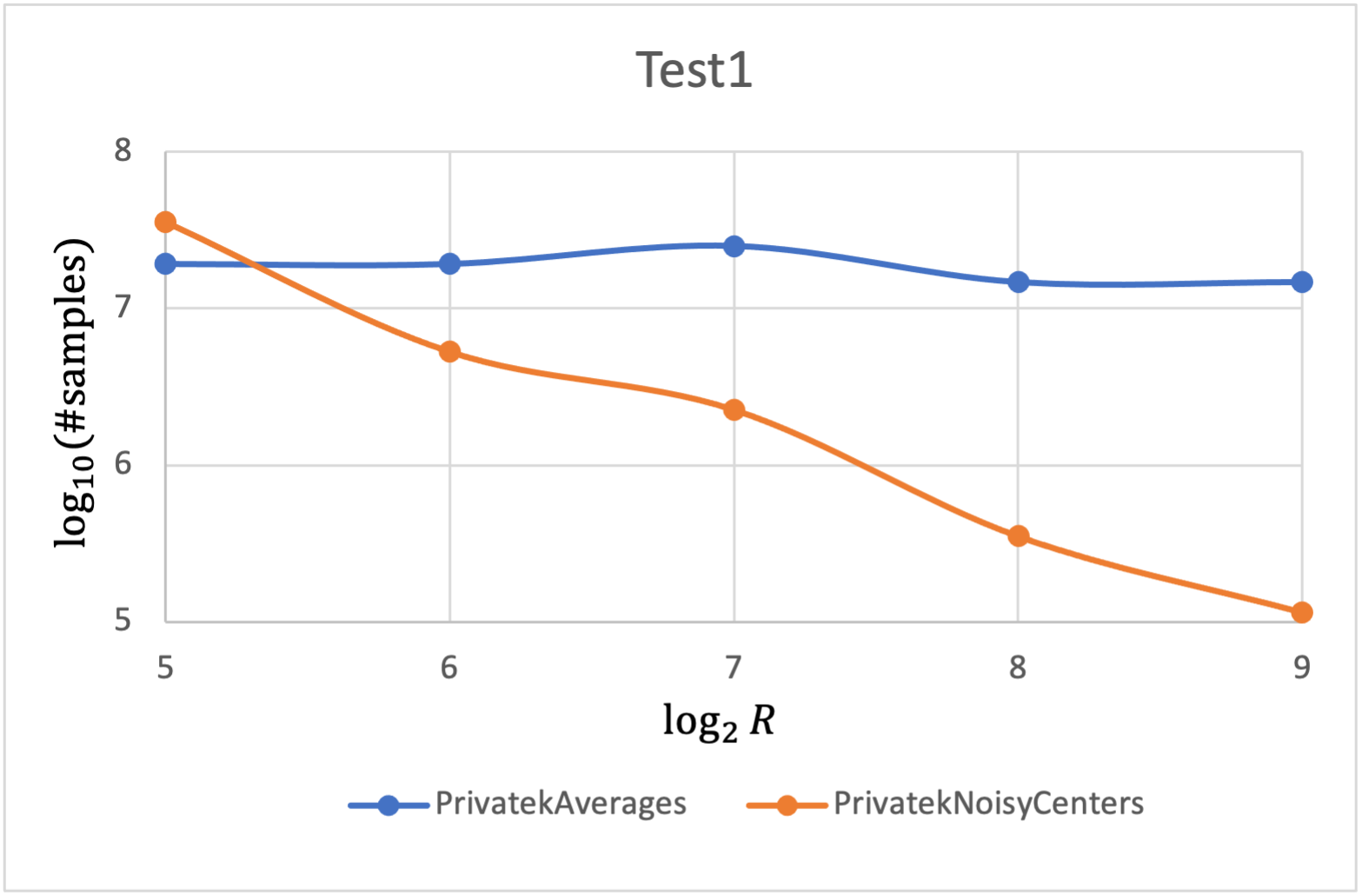
Figure 1: The case $d=1$ and $k=2$, for varies $R$.

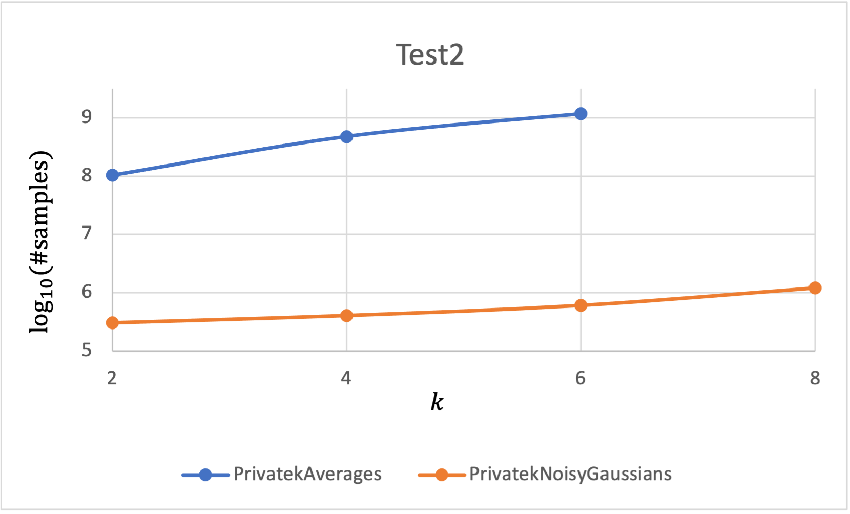
Figure 2: The case $d=4$ and $R=512\cdot k$, for varies $k$.

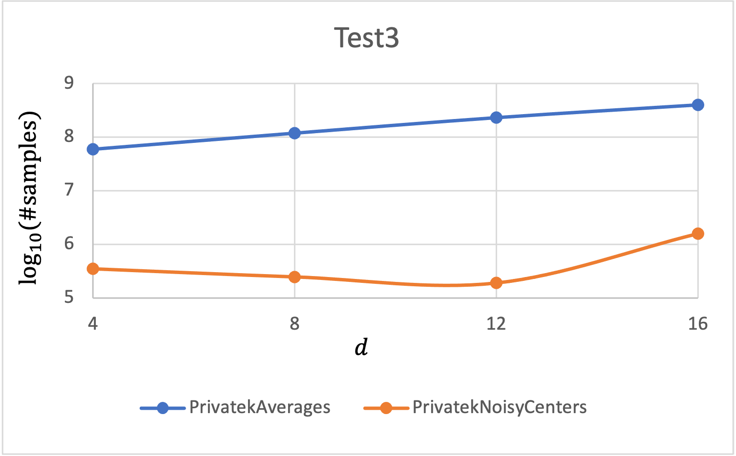
Figure 3: The case $k=2$, $R=256\sqrt{d}$, for varies $d$.

The graphs show the main bottleneck of Algorithm $\mathsf{PrivatekAverages}$ in practice. It requires only $O_{\varepsilon,\delta}(kd)$ tuples (or $O_{\varepsilon,\delta}(k\sqrt{d})$ for large values of $d$) in order to succeed, but the hidden constant is $\approx 500,000$ for our choice of $\varepsilon$ and $\delta$, and this does not improve even when the assumed separation $R$ is very large. The cause of this large constant is the group privacy of size $O(k\ell)$ that we do in Step 5a, where recall that $\ell=O\mathopen{}\mathclose{{}\left(\frac{\log^{2}(1/\delta)}{\varepsilon\log n}}\right)$ (Section 4.2.1). While in theory this $\ell$ is relatively small, with our choice of parameters we get $\ell\approx 1000$. This means that we need to execute the private average algorithm with $\hat{\varepsilon}\approx\frac{\varepsilon}{4000k}$. Internally, this $\hat{\varepsilon}$ is shared between other private algorithms, and in particular, with an Interior Point algorithm that is one of the internal components of the average algorithm from Section 2.2.6. This algorithm is implemented using the exponential mechanism [MT07], which simply outputs a random noise when the number of points is too small.

We remark that prior work on differentially-private clustering, including in ”easy” settings, is primarily theoretical. In particular, we are not aware of implemented methods that we could use as a baseline. As a sanity check, we did consider the following naive baseline: For every sample point, add a Gaussian noise to make it private. Now, the resulting noisy samples are just samples from a new Gaussian mixture. Then, run an off-the-shelf non-private method to learn the parameters of this mixture. We tested this naive method on the simple case $d=1$ and $k=2$, where we generated samples from a mixture of standard Gaussians that are separated by $R=512$. By the Gaussian mechanism, the noise magnitude that we need to add to each point for guaranteeing $(\varepsilon,\delta)$-differential privacy, is $\sigma\approx\frac{\Lambda}{\varepsilon}\sqrt{\log(1/\delta)}\gg 1$ for some $\Lambda>R$, meaning that the resulting mixture consists of very close Gaussians. We applied GaussianMixture from the package sklearn.mixture to learn this mixture, but it failed even when we used $100M$ samples, as this method is not intended for learning such close Gaussians. We remark that there are other non-private methods that are designed to learn any mixture of Gaussians (even very weakly separated ones) using enough samples (e.g., [SOAJ14]). The sample complexity and running time of these methods, however, are much worse than ours even asymptotically (e.g., the running time of [SOAJ14] is exponential in $k$), and moreover, we are not aware of any implementation we could use.

8 Conclusion

We developed an approach to bridge the gap between the theory and practice of differentially private clustering methods. For future, we hope to further optimize the ”constants” in the $k$-tuple clustering algorithms, making the approach practical for instances with lower separation. Tangentially, the inherent limitations of private versus non-private clustering suggest exploring different rigorous notions of privacy in the context of clustering.

Appendix A Additional Preliminaries

A.1 Additional Facts About Differential Privacy

A.1.1 The Exponential Mechanism

We next describe the Exponential Mechanism of [MT07]. Let ${\cal X}$ be a domain and ${\cal H}$ a set of solutions. Given a database ${\cal S}\in{\cal X}^{*}$, the Exponential Mechanism privately chooses a “good” solution $h$ out of the possible set of solutions ${\cal H}$. This “goodness” is quantified using a quality function that matches solutions to scores.

Definition .

(Quality function) A quality function is a function $q\colon{\cal X}^{*}\times{\cal H}\mapsto{\mathbb{R}}$ that maps a database ${\cal S}\in{\cal X}^{*}$ and a solution $h\in{\cal H}$ to a real number, identified as the score of the solution $h$ w.r.t the database ${\cal S}$.

Given a quality function $q$ and a database ${\cal S}$, the goal is to chooses a solution $h$ approximately maximizing $q({\cal S},h)$. The Exponential Mechanism chooses a solution probabilistically, where the probability mass that is assigned to each solution $h$ increases exponentially with its quality $q({\cal S},h)$:

Definition .

(The Exponential Mechanism) Given input parameter $\varepsilon$, finite solution set ${\cal H}$, database ${\cal S}\in{\cal X}^{m}$, and a sensitivity $1$ quality function $q$, choose randomly $h\in{\cal H}$ with probability proportional to $\exp(\varepsilon\cdot q({\cal S},h)/2)$.

Proposition .

(Properties of the Exponential Mechanism) (i) The Exponential Mechanism is $\varepsilon$-differentially private. (ii) Let $\hat{e}:=\max_{f\in{\cal H}}\{q({\cal S},f)\}$ and $\Delta>0$. The Exponential Mechanism outputs a solution $h$ such that $q({\cal S},h)\leq\hat{e}-\Delta$ with probability at most $\mathopen{}\mathclose{{}\left|{\cal H}}\right|\cdot\exp\mathopen{}\mathclose{{}\left(-\varepsilon\Delta/2}\right)$.

A.1.2 Private Interior Point and Bounding Segment in ${\mathbb{R}}$

Proposition (Finding an Interior Point in ${\mathbb{R}}$).

Let $\varepsilon\in(0,1)$, $\Lambda>0$ and $g\in[0,\Lambda]$. There exists an efficient $\varepsilon$-differentially private algorithm that takes an $n$-size database ${\cal S}$ of numbers in the segment $[-\Lambda,\Lambda]$ and outputs a number $z\in[-\Lambda,\Lambda]$ that with probability $1-2(\Lambda/g+1)\cdot\exp\mathopen{}\mathclose{{}\left(-\varepsilon n/4}\right)$ it holds that $z\in[\min({\cal S})-g,\max({\cal S})+g]$. The algorithm runs in time $\tilde{O}\mathopen{}\mathclose{{}\left(n}\right)$ (ignoring $\log\mathopen{}\mathclose{{}\left(\frac{n\Delta}{g}}\right)$ factors).

Proof.

Define the grid $G=\{-\Lambda,-\Lambda+g,\ldots,-\Lambda+\mathopen{}\mathclose{{}\left\lceil\frac{2\Lambda}{g}}\right\rceil\cdot g\}$, and for every $x\in G$ let ${\rm left}(x)=-\Lambda+\mathopen{}\mathclose{{}\left\lfloor\frac{x+\Lambda}{g}}\right\rfloor\cdot g$ (i.e., the closest grid point to $x$ from the left side) and ${\rm right}(x)=-\Lambda+\mathopen{}\mathclose{{}\left\lceil\frac{x+\Lambda}{g}}\right\rceil\cdot g$ (i.e., the closest grid point to $x$ from the right side). Now, apply the exponential mechanism (A.1.1) with the quality function

$$\forall y\in G\colon\quad q({\cal S},y)=\min\{\mathopen{}\mathclose{{}\left|\{x\in{\cal S}\colon{\rm left}(x)\leq y\}}\right|,\mathopen{}\mathclose{{}\left|\{x\in{\cal S}\colon{\rm right}(x)\geq y\}}\right|\}$$

For the utility analysis, let $m$ be the median of ${\cal S}$, and note that $q({\cal S},{\rm left}(m)),q({\cal S},{\rm right}(m))\geq n/2$. Therefore, by Section A.1.1, with probability $\geq 1-\mathopen{}\mathclose{{}\left|G}\right|\cdot\exp\mathopen{}\mathclose{{}\left(-\varepsilon n/4}\right)\geq 1-2(\Lambda/g+1)\cdot\exp\mathopen{}\mathclose{{}\left(-\varepsilon n/4}\right)$, the mechanism outputs a point $z$ with $q(S,z)>0$, which yields in particular that $z\in[\min({\cal S})-g,\max({\cal S})+g]$.

For the running time analysis, we implement the sampling as follows: For $x\in{\cal S}$ we let $A_{x}=\{{\rm left}(x)-g,{\rm left}(x),{\rm right}(x),{\rm right}(x)+g\}$, and let $A=\cup_{x\in{\cal S}}A_{x}$. Note that for every consecutive grid points $y,y^{\prime}=y+g\in G$ with $q({\cal S},y)\neq q({\cal S},y^{\prime})$, it holds that $y,y^{\prime}\in A$: If $q({\cal S},y)>q({\cal S},y^{\prime})$, there must exist $x\in{\cal S}$ such that $x\in(y-g,y]$, yielding that $y\in[x,x+g)\implies y={\rm right}(x),y^{\prime}={\rm right}(x)+g$. Otherwise (i.e., $q({\cal S},y)<q({\cal S},y^{\prime})$), there must exist $x\in{\cal S}$ such that $x\in[y^{\prime},y^{\prime}+g)$, yielding that $y^{\prime}\in(x-g,x]\implies y^{\prime}={\rm left}(x),y={\rm left}(x)-g$.

Then, we sort $A$ in time $\tilde{O}(n)$, and let $a_{1}\leq\ldots\leq a_{m}$ be the sorted elements in $A$ (recall that $m=\mathopen{}\mathclose{{}\left|A}\right|\leq 4n$). For each $i\in[m+1]$, we compute $w({\cal S},a_{i})=q({\cal S},a_{i})\cdot\mathopen{}\mathclose{{}\left|G\cap(a_{i-1},a_{i}]}\right|$ (i.e., $w({\cal S},a_{i})$ is the the original quality of $a_{i}$ times the number of grid points in $(a_{i-1},a_{i}]$, where $a_{0}=-\Lambda-g$ and $a_{m+1}=\Lambda+g$), and choose a value $a_{i}$ with probability $\propto w({\cal S},a_{i})$. Note that the computation of each $w({\cal S},a_{i})$ can be done in time $\tilde{O}(1)$ using simple binary searches over the (sorted) multisets ${\cal S}_{{\rm left}}=\cup_{x\in{\cal S}}\{{\rm left}(x)\}$ and ${\cal S}_{{\rm right}}=\cup_{x\in{\cal S}}\{{\rm right}(x)\}$ (a “multiset” union, that includes duplications).

Finally, given the chosen $a_{i}$ from the mechanism, it is left to sample a uniform point in $G\cap(a_{i-1},a_{i}]$ (since we know, by the property of $A$, that all the point there have the same value of $q({\cal S},\cdot)$). This can be easily implemented in time $O(\log\mathopen{}\mathclose{{}\left|G}\right|)=\tilde{O}(1)$.     $\Box$

Proposition (Finding a Bounding Segment of Points in ${\mathbb{R}}$).

Let $\beta,\varepsilon\in(0,1)$, $\Lambda>0$ and $g\in[0,\Lambda]$. There exists an efficient $\varepsilon$-differentially private algorithm that takes an $n$-size database ${\cal S}$ of numbers in the segment $[-\Lambda,\Lambda]$ and outputs a segment $[x,y]$ such that with probability at least $1-\beta$ the following holds:

• $\mathopen{}\mathclose{{}\left|{\cal S}\cap[x,y]}\right|\geq n-\frac{8}{\varepsilon}\log\mathopen{}\mathclose{{}\left(\frac{4\Lambda}{g\beta}}\right)-2$ (i.e., the segment contain most of the points in ${\cal S}$), and

• $y-x\leq\max({\cal S})-\min({\cal S})+4g$.

The algorithm runs in time $\tilde{O}\mathopen{}\mathclose{{}\left(n}\right)$ (ignoring $\log\mathopen{}\mathclose{{}\left(\frac{n\Delta}{\varepsilon\beta g}}\right)$ factors).

Proof.

In the following assume that $n\geq\frac{8}{\varepsilon}\log\mathopen{}\mathclose{{}\left(\frac{4\Lambda}{g\beta}}\right)+2$ (otherwise the proof trivially holds for any segment $[x,x]$). Let ${\cal S}_{0}$ be the smallest $\frac{4}{\varepsilon}\log\mathopen{}\mathclose{{}\left(\frac{4\Lambda}{g\beta}}\right)+1$ points in ${\cal S}$, and let ${\cal S}_{1}$ be the largest $\frac{4}{\varepsilon}\log\mathopen{}\mathclose{{}\left(\frac{4\Lambda}{g\beta}}\right)+1$ points in ${\cal S}$. For each $b\in\{0,1\}$ apply Section A.1.2 (interior point) on ${\cal S}_{b}$ for finding a number $z_{b}\in[-\Lambda,\Lambda]$ that belongs to $[\min({\cal S}_{b})-g,\max({\cal S}_{b})+g]$ with probability at least $1-2(\Lambda/g+1)\cdot\exp\mathopen{}\mathclose{{}\left(-\varepsilon\mathopen{}\mathclose{{}\left|{\cal S}_{b}}\right|/4}\right)\geq 1-\beta/2$. Therefore, by setting $x=z_{0}-g$ and $y=z_{1}+g$ we get that with probability $1-\beta$ it holds that: (1) $[\max({\cal S}_{0}),\min({\cal S}_{1})]\subseteq[x,y]$ and that (2) $[x,y]\subseteq[\min({\cal S}_{0})-2g,\max({\cal S}_{1})+2g]=[\min({\cal S})-2g,\max({\cal S})+2g]$. By (1) we get that all points in ${\cal S}$ expect (at most) $(\mathopen{}\mathclose{{}\left|{\cal S}_{0}}\right|-1)+(\mathopen{}\mathclose{{}\left|{\cal S}_{1}}\right|-1)\leq\frac{8}{\varepsilon}\log\mathopen{}\mathclose{{}\left(\frac{4\Lambda}{g\beta}}\right)$ are inside $[x,y]$, and by (2) we get that $y-x\geq\max({\cal S})-\min({\cal S})+4g$, as required.

For the running time analysis, note that by sorting ${\cal S}$ we can determine ${\cal S}_{0}$ and ${\cal S}_{1}$ in time $\tilde{O}(n)$, and the cost of executing the algorithm from Section A.1.2 on each ${\cal S}_{b}$ is $\tilde{O}\mathopen{}\mathclose{{}\left(\frac{1}{\varepsilon}}\right)=\tilde{O}\mathopen{}\mathclose{{}\left(n}\right)$.     $\Box$

A.1.3 Estimating the Average of Points

Proposition (Estimating the Average of Bounded Points in ${\mathbb{R}}$).

Let $\beta,\varepsilon,\delta\in(0,1)$, $\Lambda>0$ and $r_{\min}\in[0,\Lambda]$. There exists an efficient $(\varepsilon,\delta)$-differentially private algorithm that takes an $n$-size database ${\cal S}$ of numbers in the segment $[-\Lambda,\Lambda]$ and satisfy the following utility guarantee: If $n\geq\frac{16}{\varepsilon}\log\mathopen{}\mathclose{{}\left(\frac{4\Lambda}{r_{\min}\beta}}\right)+4$, then with probability $1-\beta$, the algorithm outputs a number $\hat{a}\in{\mathbb{R}}$ such that

$$\mathopen{}\mathclose{{}\left|\hat{a}-{\rm Avg}({\cal S})}\right|\leq O\mathopen{}\mathclose{{}\left(\frac{\max\{r,r_{\min}\}}{\varepsilon n}\mathopen{}\mathclose{{}\left(\sqrt{\log(1/\delta)\log(1/\beta)}+\log\mathopen{}\mathclose{{}\left(\frac{\Lambda}{r_{\min}\beta}}\right)}\right)}\right),$$

where $r=\max({\cal S})-\min({\cal S})$. The algorithm runs in time $\tilde{O}(n)$ (ignoring $\log\mathopen{}\mathclose{{}\left(\frac{n\Delta}{r_{\min}\varepsilon\beta}}\right)$ factors).

Proof.

The algorithm does the following: (1) Privately find a bounding segment $[x,y]$ using Section A.1.2 with parameters $\beta/2,\varepsilon/2,g=r_{\min},\Lambda$, let $\hat{r}=y-x$ and let ${\cal S}^{\prime}={\cal S}\cap[x,y]$ (2) Use the ($1$-dimensional) Gaussian mechanism (Theorem 2.4) with $\lambda=\frac{\hat{r}}{\mathopen{}\mathclose{{}\left|{\cal S}^{\prime}}\right|}$ and parameters $\beta/2,\varepsilon/2,\delta$ for computing a noisy average $\hat{a}$ of ${\cal S}^{\prime}$ (see Section 2.2.5). By the properties of the Gaussian mechanism (see Section 2.2.5) along with basic composition it holds that the above algorithm is $(\varepsilon,\delta)$-differentially private. For the utility analysis, note that with probability $1-\beta$, the segment $[x,y]$ satisfies the conditions of Section A.1.2 and the noise added to the average in the second step is at most $O\mathopen{}\mathclose{{}\left(\frac{\hat{r}}{\varepsilon\mathopen{}\mathclose{{}\left|{\cal S}^{\prime}}\right|}\sqrt{\log(1/\delta)\log(1/\beta)}}\right)$. In the rest of the analysis we assume that this event occurs. Now, by definition of $r$, it holds that

$$\mathopen{}\mathclose{{}\left|{\rm Avg}(S)-{\rm Avg}({\cal S}^{\prime})}\right|\leq\frac{r\mathopen{}\mathclose{{}\left|{\cal S}\setminus{\cal S}^{\prime}}\right|}{n}\leq\frac{8r}{\varepsilon n}\log\mathopen{}\mathclose{{}\left(\frac{2\Lambda}{r_{\min}\beta}}\right)+\frac{2r}{n}$$

Moreover, it holds that

$$\mathopen{}\mathclose{{}\left|\hat{a}-{\rm Avg}({\cal S}^{\prime})}\right|\leq O\mathopen{}\mathclose{{}\left(\frac{\hat{r}}{\varepsilon\mathopen{}\mathclose{{}\left|{\cal S}^{\prime}}\right|}\sqrt{\log(1/\delta)\log(1/\beta)}}\right)\leq O\mathopen{}\mathclose{{}\left(\frac{\max\{r,r_{\min}\}}{\varepsilon n}\sqrt{\log(1/\delta)\log(1/\beta)}}\right),$$

where the second inequality holds since $\hat{r}\leq r+4r_{\min}$ and $\mathopen{}\mathclose{{}\left|{\cal S}^{\prime}}\right|\geq n/2$ by the assumption on $n$. The proof now follow by the above two inequalities.

For the running time analysis, step (1) takes $\tilde{O}(n)$ time (Section A.1.2). Step (2) that executes the Gaussian Mechanism, takes $\tilde{O}(n)$ time for computing the average, and $\tilde{O}(1)$ for sampling a number from a single one-dimensional.     $\Box$

Proposition (Estimating the Average of Bounded Points in ${\mathbb{R}}^{d}$ (Restatement of Section 2.2.6)).

Let $\varepsilon\in(0,1)$, $d,\Lambda>0$ and let $r_{\min}\in[0,\Lambda]$. There exists an efficient $(\varepsilon,\delta)$-differentially private algorithm that takes an $n$-size database ${\cal S}$ of points inside the ball $B({\bf 0},\Lambda)$ in ${\mathbb{R}}^{d}$ and satisfy the following utility guarantee: Assume that $n\geq\frac{32\sqrt{2d\log(2/\delta)}}{\varepsilon}\log\mathopen{}\mathclose{{}\left(\frac{4d\Lambda}{r_{\min}\beta}}\right)+4$, and let $r>0$ be the minimal radius of a $d$-dimensional ball that contains all points in ${\cal S}$. Then with probability $1-\beta$, the algorithm outputs $\hat{{\bf a}}\in{\mathbb{R}}^{d}$ such that

$$\mathopen{}\mathclose{{}\left\lVert\hat{{\bf a}}-{\rm Avg}({\cal S})}\right\rVert\leq O\mathopen{}\mathclose{{}\left(\max\{r,r_{\min}\}\cdot\frac{d\sqrt{\log(1/\delta)}}{\varepsilon n}\mathopen{}\mathclose{{}\left(\sqrt{\log(d/\delta)\log(d/\beta)}+\log\mathopen{}\mathclose{{}\left(\frac{\Lambda d}{r_{\min}\beta}}\right)}\right)}\right).$$

The algorithm runs in time $\tilde{O}(dn)$ (ignoring logarithmic factors).

Proof.

The algorithm does the following: For each $i\in[d]$, let ${\cal S}_{i}=\{x_{i}\colon(x_{1},\ldots,x_{d})\in{\cal S}\}$ and compute an estimation $\hat{a}_{i}$ of ${\rm Avg}({\cal S}_{i})$ (in time $\tilde{O}(n)$) by applying Section A.1.3 with parameters $r_{\min},\Lambda$, $\tilde{\varepsilon}=\frac{\varepsilon}{2\sqrt{2d\log(2/\delta)}}$, $\tilde{\delta}=\frac{\delta}{d}$, $\tilde{\beta}=\frac{\beta}{d}$. Finally, output $\hat{{\bf a}}=(\hat{a}_{1},\ldots,\hat{a}_{d})$. It is clear by advanced composition (Theorem 2.2) that the algorithm is $(\varepsilon,\delta)$-differentially private. For the utility guarantee, note that with probability at least $1-\beta$, for every $i\in[d]$ it holds that

$$\mathopen{}\mathclose{{}\left|\hat{a}_{i}-{\rm Avg}({\cal S}_{i})}\right| \leq O\mathopen{}\mathclose{{}\left(\frac{r}{\tilde{\varepsilon}n}\mathopen{}\mathclose{{}\left(\sqrt{\log(1/\tilde{\delta})\log(1/\tilde{\beta})}+\log\mathopen{}\mathclose{{}\left(\frac{\Lambda}{r_{\min}\tilde{\beta}}}\right)}\right)}\right)$$

$$=O\mathopen{}\mathclose{{}\left(\frac{r\sqrt{d\log(1/\delta)}}{\varepsilon n}\mathopen{}\mathclose{{}\left(\sqrt{\log(d/\delta)\log(d/\beta)}+\log\mathopen{}\mathclose{{}\left(\frac{\Lambda d}{r_{\min}\beta}}\right)}\right)}\right),$$

and hence

$$\mathopen{}\mathclose{{}\left\lVert\hat{{\bf a}}-{\rm Avg}({\cal S})}\right\rVert =\sqrt{\sum_{i=1}^{d}(\hat{a}_{i}-{\rm Avg}({\cal S}_{i}))^{2}}$$

$$\leq O\mathopen{}\mathclose{{}\left(\frac{rd\sqrt{\log(1/\delta)}}{\varepsilon n}\mathopen{}\mathclose{{}\left(\sqrt{\log(d/\delta)\log(d/\beta)}+\log\mathopen{}\mathclose{{}\left(\frac{\Lambda d}{r_{\min}\beta}}\right)}\right)}\right)$$

$\Box$

Remark .

The above two algorithms guarantee differential-privacy whenever two neighboring databases have equal size. However, they can be easily extended to a more general case in which the privacy guarantee also holds in cases of addition and deletion of a point, by extending the Gaussian mechanism used in Section A.1.3 (see Section 2.2.5) with essentially the same noise magnitude.

Appendix B Missing Proofs

B.1 Proving Section 5.1

In this section we prove Section 5.1, restated below

Proposition (Restatement of Section 5.1).

Let ${\cal P}$ be a multiset of $n$ points in ${\cal B}({\bf 0},\Lambda)\subseteq{\mathbb{R}}^{d}$ and let ${\cal A}$ be an $\omega$-approximation algorithm for $k$-means. Consider the following random execution: (1) Construct a multiset ${\cal S}$ of $s$ i.i.d. samples from ${\cal P}$, (2) Compute $\tilde{C}={\cal A}({\cal S},k)$. Then for every $\beta>0$, with probability $1-\beta$ it holds that

$${\rm COST}_{{\cal P}}(\tilde{C})\leq\omega\cdot{\rm OPT}_{k}({\cal P})+\xi(s,\beta),$$

where $\xi(s,\beta):=4\mathopen{}\mathclose{{}\left(M(s,\beta)+\sqrt{M(s,\beta)\cdot\omega{\rm OPT}_{k}({\cal P})}}\right)$ for $M(s,\beta):=25\Lambda^{2}kd\log\mathopen{}\mathclose{{}\left(\frac{2nd}{\beta}}\right)\cdot\frac{n}{s}$.

In the following, fix values of $s$ and $\beta$, let $\xi=\xi(s,\beta)$ and $M=M(s,\beta)$. The following event and claims are with respect to the random process in Section 5.1.

Claim (Event $E$ [SSS20]).

Let $E$ be the event that for every $C\in B(0,\Lambda)^{k}$, we have that

$$\mathopen{}\mathclose{{}\left|\frac{n}{s}\cdot{\rm COST}_{{\cal S}}(C)-{\rm COST}_{{\cal P}}(C)}\right|\leq\sqrt{M\cdot{\rm COST}_{{\cal P}}(C)}:=\Delta(C)$$

Then it holds that ${\mathrm{Pr}}\mathopen{}\mathclose{{}\left[E}\right]\geq 1-\beta$.

We next prove some useful facts that holds when event $E$ occurs.

Claim .

Conditioned on event $E$, it holds that

$${\rm COST}_{{\cal P}}(\tilde{C})\leq\omega\cdot{\rm OPT}_{k}({\cal P})+\Delta(C^{*}_{{\cal P}})+\Delta(\tilde{C}),$$

letting $\tilde{C}$ be the set from Section 5.1, and letting $C^{*}_{{\cal P}}$ be the optimal $k$-means of ${\cal P}$.

Proof.

Let $C^{*}_{{\cal S}}$ be the optimal $k$-means of ${\cal S}$. By the assumption on the algorithm $\mathsf{A}$, the set $\tilde{C}$ satisfies ${\rm COST}_{{\cal S}}(\tilde{C})\leq\omega\cdot{\rm OPT}_{k}({\cal S})$. The proof follows by the following calculation

$${\rm COST}_{{\cal P}}(\tilde{C}) \leq\frac{n}{s}\cdot{\rm COST}_{{\cal S}}(\tilde{C})+\Delta(\tilde{C})$$

$$\leq\omega\cdot\frac{n}{s}\cdot{\rm COST}_{{\cal S}}(C^{*}_{{\cal S}})+\Delta(\tilde{C})$$

$$\leq\omega\cdot\frac{n}{s}\cdot{\rm COST}_{{\cal S}}(C^{*}_{{\cal P}})+\Delta(\tilde{C})$$

$$\leq\omega\cdot\frac{n}{s}\cdot\mathopen{}\mathclose{{}\left(\frac{m}{n}\cdot{\rm COST}_{{\cal P}}(C^{*}_{{\cal P}})+\frac{s}{n}\cdot\Delta(C^{*}_{{\cal P}})}\right)+\Delta(\tilde{C})$$

$$=\omega\cdot{\rm OPT}_{k}({\cal P})+\Delta(C^{*}_{{\cal P}})+\Delta(\tilde{C}),$$

where the third inequality holds by event $E$,     $\Box$

We now prove a corollary of Section B.1.

Corollary .

Conditioned on event $E$, it holds that

$$\Delta(\tilde{C})\leq 2\mathopen{}\mathclose{{}\left(M+\sqrt{M\omega{\rm OPT}_{k}({\cal P})}}\right)$$

Proof.

Let $x=\Delta(\tilde{C})=\sqrt{M\cdot{\rm COST}_{{\cal P}}(\tilde{C})}$. By Section B.1, it holds that

$$\frac{x^{2}}{M}-x\leq\omega\cdot{\rm OPT}_{k}({\cal P})+\sqrt{M\cdot{\rm OPT}_{k}({\cal P})}.$$

Since $x\geq 0$, we conclude that

$$x \leq\frac{1}{2}\cdot\mathopen{}\mathclose{{}\left(M+\sqrt{M^{2}+4M\omega{\rm OPT}_{k}({\cal P})+4M^{1.5}\sqrt{{\rm OPT}_{k}({\cal P})}}}\right)$$

$$\leq M+\sqrt{M\omega{\rm OPT}_{k}({\cal P})}+M^{0.75}\cdot{\rm OPT}_{k}({\cal P})^{1/4}$$ (13)

$$\leq 2\mathopen{}\mathclose{{}\left(M+\sqrt{M\omega{\rm OPT}_{k}({\cal P})}}\right),$$

where the second inequality holds by the fact that $\sqrt{a+b}\leq\sqrt{a}+\sqrt{b}$ for $a,b\geq 0$, and the last inequality holds since the third term in (B.1) is either smaller than the first term, or smaller than the second one (recall that $M\geq 1$).     $\Box$

The proof of Section 5.1 now immediately follows by Section B.1 and Section B.1.

B.2 Proving Section 5.1

Proposition (Restatement of Section 5.1).

Let $k\in{\mathbb{N}}$ and $\gamma\in[0,1/8]$. Let ${\cal P}\in({\mathbb{R}}^{d})^{*}$, let $C=\{{\bf c}_{1},\ldots,{\bf c}_{k}\}$ and $C^{\prime}=\{{\bf c}_{1}^{\prime},\ldots,{\bf c}_{k}^{\prime}\}$ be two $k$-tuples of centers in ${\mathbb{R}}^{d}$ such that for every $i\in[k]$ it holds that $\mathopen{}\mathclose{{}\left\lVert{\bf c}_{i}^{\prime}-{\bf c}_{i}}\right\rVert\leq\gamma\cdot D_{i}$, where $D_{i}=\min_{j\neq i}\mathopen{}\mathclose{{}\left\lVert{\bf c}_{i}-{\bf c}_{j}}\right\rVert$. In addition, for every $i\in[k]$ let ${\cal P}_{i}$ be the multiset of all points in ${\cal P}$ that ${\bf c}_{i}^{\prime}$ is closest to them in $C^{\prime}$. Then

$$\sum_{i=1}^{k}{\rm OPT}_{1}({\cal P}_{i})\leq(1+32\gamma){\rm COST}_{{\cal P}}(C).$$

Proof.

In the following, for ${\bf x}\in{\cal P}$ let $i_{{\bf x}}=\operatorname*{argmin}_{i}\{\mathopen{}\mathclose{{}\left\lVert{\bf x}-{\bf c}_{i}}\right\rVert\}$ (i.e., the index of the closest center to ${\bf x}$ in $C$), and let $j_{{\bf x}}=\operatorname*{argmin}_{j}\{\mathopen{}\mathclose{{}\left\lVert{\bf x}-{\bf c}_{j}^{\prime}}\right\rVert\}$ (i.e., the index of the closest center to ${\bf x}$ in $C^{\prime}$). It holds that

$$\sum_{i=1}^{k}{\rm OPT}_{1}({\cal P}_{i}) \leq\sum_{i=1}^{k}\sum_{{\bf x}\in{\cal P}_{i}}\mathopen{}\mathclose{{}\left\lVert{\bf x}-{\bf c}_{i}}\right\rVert^{2}$$

$$=\sum_{{\bf x}\in{\cal P}}\mathopen{}\mathclose{{}\left\lVert{\bf x}-{\bf c}_{j_{{\bf x}}}}\right\rVert^{2}$$

$$=\sum_{{\bf x}\in{\cal P}}\mathopen{}\mathclose{{}\left\lVert{\bf x}-{\bf c}_{i_{{\bf x}}}}\right\rVert^{2}+\sum_{{\bf x}\in{\cal P}}\mathopen{}\mathclose{{}\left(\mathopen{}\mathclose{{}\left\lVert{\bf x}-{\bf c}_{j_{{\bf x}}}}\right\rVert^{2}-\mathopen{}\mathclose{{}\left\lVert{\bf x}-{\bf c}_{i_{{\bf x}}}}\right\rVert^{2}}\right)$$

$$={\rm COST}_{{\cal P}}(C)+\sum_{{\bf x}\in{\cal P}}\mathopen{}\mathclose{{}\left(\mathopen{}\mathclose{{}\left\lVert{\bf x}-{\bf c}_{j_{{\bf x}}}}\right\rVert^{2}-\mathopen{}\mathclose{{}\left\lVert{\bf x}-{\bf c}_{i_{{\bf x}}}}\right\rVert^{2}}\right)$$

In the following, fix ${\bf x}\in{\cal P}$. We now bound

$$\mathopen{}\mathclose{{}\left\lVert{\bf x}-{\bf c}_{j_{{\bf x}}}}\right\rVert^{2}-\mathopen{}\mathclose{{}\left\lVert{\bf x}-{\bf c}_{i_{{\bf x}}}}\right\rVert^{2}=\mathopen{}\mathclose{{}\left(\mathopen{}\mathclose{{}\left\lVert{\bf x}-{\bf c}_{j_{{\bf x}}}}\right\rVert-\mathopen{}\mathclose{{}\left\lVert{\bf x}-{\bf c}_{i_{{\bf x}}}}\right\rVert}\right)\mathopen{}\mathclose{{}\left(\mathopen{}\mathclose{{}\left\lVert{\bf x}-{\bf c}_{j_{{\bf x}}}}\right\rVert+\mathopen{}\mathclose{{}\left\lVert{\bf x}-{\bf c}_{i_{{\bf x}}}}\right\rVert}\right)$$

First, since $\mathopen{}\mathclose{{}\left\lVert{\bf x}-{\bf c}_{j_{{\bf x}}}^{\prime}}\right\rVert\leq\mathopen{}\mathclose{{}\left\lVert{\bf x}-{\bf c}_{i_{{\bf x}}}^{\prime}}\right\rVert$ it holds that

$$\mathopen{}\mathclose{{}\left\lVert{\bf x}-{\bf c}_{j_{{\bf x}}}}\right\rVert\leq\mathopen{}\mathclose{{}\left\lVert{\bf x}-{\bf c}_{j_{{\bf x}}}^{\prime}}\right\rVert+\mathopen{}\mathclose{{}\left\lVert{\bf c}_{j_{{\bf x}}}^{\prime}-{\bf c}_{j_{{\bf x}}}}\right\rVert\leq\mathopen{}\mathclose{{}\left\lVert{\bf x}-{\bf c}_{i_{{\bf x}}}^{\prime}}\right\rVert+\gamma\mathopen{}\mathclose{{}\left\lVert{\bf c}_{i_{{\bf x}}}-{\bf c}_{j_{{\bf x}}}}\right\rVert$$ (14)

Second,

$$\mathopen{}\mathclose{{}\left\lVert{\bf x}-{\bf c}_{i_{{\bf x}}}}\right\rVert\geq\mathopen{}\mathclose{{}\left\lVert{\bf x}-{\bf c}_{i_{{\bf x}}}^{\prime}}\right\rVert-\mathopen{}\mathclose{{}\left\lVert{\bf c}_{i_{{\bf x}}}^{\prime}-{\bf c}_{i_{{\bf x}}}}\right\rVert\geq\mathopen{}\mathclose{{}\left\lVert{\bf x}-{\bf c}_{i_{{\bf x}}}^{\prime}}\right\rVert-\gamma\mathopen{}\mathclose{{}\left\lVert{\bf c}_{i_{{\bf x}}}-{\bf c}_{j_{{\bf x}}}}\right\rVert$$

Therefore

$$\mathopen{}\mathclose{{}\left\lVert{\bf x}-{\bf c}_{j_{{\bf x}}}}\right\rVert-\mathopen{}\mathclose{{}\left\lVert{\bf x}-{\bf c}_{i_{{\bf x}}}}\right\rVert\leq 2\gamma\mathopen{}\mathclose{{}\left\lVert{\bf c}_{i_{{\bf x}}}-{\bf c}_{j_{{\bf x}}}}\right\rVert$$

Now, $\mathopen{}\mathclose{{}\left\lVert{\bf x}-{\bf c}_{i_{{\bf x}}}}\right\rVert\leq\mathopen{}\mathclose{{}\left\lVert{\bf x}-{\bf c}_{j_{{\bf x}}}}\right\rVert$ and therefore

$$\mathopen{}\mathclose{{}\left\lVert{\bf x}-{\bf c}_{j_{{\bf x}}}}\right\rVert+\mathopen{}\mathclose{{}\left\lVert{\bf x}-{\bf c}_{i_{{\bf x}}}}\right\rVert \leq 2\mathopen{}\mathclose{{}\left\lVert{\bf x}-{\bf c}_{j_{{\bf x}}}}\right\rVert$$

$$\leq 2\mathopen{}\mathclose{{}\left\lVert{\bf x}-{\bf c}_{i_{{\bf x}}}^{\prime}}\right\rVert+2\gamma\mathopen{}\mathclose{{}\left\lVert{\bf c}_{i_{{\bf x}}}-{\bf c}_{j_{{\bf x}}}}\right\rVert$$

$$\leq 2\mathopen{}\mathclose{{}\left(\mathopen{}\mathclose{{}\left\lVert{\bf x}-{\bf c}_{i_{{\bf x}}}}\right\rVert+\mathopen{}\mathclose{{}\left\lVert{\bf c}_{i_{{\bf x}}}^{\prime}-{\bf c}_{i_{{\bf x}}}}\right\rVert}\right)+2\gamma\mathopen{}\mathclose{{}\left\lVert{\bf c}_{i_{{\bf x}}}-{\bf c}_{j_{{\bf x}}}}\right\rVert$$

$$\leq 2\mathopen{}\mathclose{{}\left\lVert{\bf x}-{\bf c}_{i_{{\bf x}}}}\right\rVert+4\gamma\mathopen{}\mathclose{{}\left\lVert{\bf c}_{i_{{\bf x}}}-{\bf c}_{j_{{\bf x}}}}\right\rVert,$$

where the second inequality holds by Equation 14.

We now like to bound $\mathopen{}\mathclose{{}\left\lVert{\bf c}_{i_{{\bf x}}}-{\bf c}_{j_{{\bf x}}}}\right\rVert$ as a function of $\mathopen{}\mathclose{{}\left\lVert{\bf x}-{\bf c}_{i_{{\bf x}}}}\right\rVert$. We first bound $\mathopen{}\mathclose{{}\left\lVert{\bf c}_{i_{{\bf x}}}-{\bf c}_{j_{{\bf x}}}}\right\rVert$ as a function of $\mathopen{}\mathclose{{}\left\lVert{\bf x}-{\bf c}_{i_{{\bf x}}}^{\prime}}\right\rVert$.

$$2\mathopen{}\mathclose{{}\left\lVert{\bf x}-{\bf c}_{i_{{\bf x}}}^{\prime}}\right\rVert \geq\mathopen{}\mathclose{{}\left\lVert{\bf x}-{\bf c}_{i_{{\bf x}}}^{\prime}}\right\rVert+\mathopen{}\mathclose{{}\left\lVert{\bf x}-{\bf c}_{j_{{\bf x}}}^{\prime}}\right\rVert$$

$$\geq\mathopen{}\mathclose{{}\left\lVert{\bf c}_{i_{{\bf x}}}^{\prime}-{\bf c}_{j_{{\bf x}}}^{\prime}}\right\rVert$$

$$\geq\mathopen{}\mathclose{{}\left\lVert{\bf c}_{i_{{\bf x}}}-{\bf c}_{j_{{\bf x}}}}\right\rVert-\mathopen{}\mathclose{{}\left\lVert{\bf c}_{i_{{\bf x}}}-{\bf c}_{i_{{\bf x}}}^{\prime}}\right\rVert-\mathopen{}\mathclose{{}\left\lVert{\bf c}_{j_{{\bf x}}}-{\bf c}_{j_{{\bf x}}}^{\prime}}\right\rVert$$

$$\geq(1-2\gamma)\mathopen{}\mathclose{{}\left\lVert{\bf c}_{i_{{\bf x}}}-{\bf c}_{j_{{\bf x}}}}\right\rVert,$$ (15)

In addition

$$\mathopen{}\mathclose{{}\left\lVert{\bf x}-{\bf c}_{i_{{\bf x}}}^{\prime}}\right\rVert\leq\mathopen{}\mathclose{{}\left\lVert{\bf x}-{\bf c}_{i_{{\bf x}}}}\right\rVert+\mathopen{}\mathclose{{}\left\lVert{\bf c}_{i_{{\bf x}}}-{\bf c}_{i_{{\bf x}}}^{\prime}}\right\rVert\leq\mathopen{}\mathclose{{}\left\lVert{\bf x}-{\bf c}_{i_{{\bf x}}}}\right\rVert+\gamma\mathopen{}\mathclose{{}\left\lVert{\bf c}_{i_{{\bf x}}}-{\bf c}_{j_{{\bf x}}}}\right\rVert$$

Therefore,

$$2\mathopen{}\mathclose{{}\left\lVert{\bf x}-{\bf c}_{i_{{\bf x}}}}\right\rVert\geq(1-4\gamma)\mathopen{}\mathclose{{}\left\lVert{\bf c}_{i_{{\bf x}}}-{\bf c}_{j_{{\bf x}}}}\right\rVert$$

We have that

$$\mathopen{}\mathclose{{}\left\lVert{\bf x}-{\bf c}_{j_{{\bf x}}}}\right\rVert^{2}-\mathopen{}\mathclose{{}\left\lVert{\bf x}-{\bf c}_{i_{{\bf x}}}}\right\rVert^{2} =\mathopen{}\mathclose{{}\left(\mathopen{}\mathclose{{}\left\lVert{\bf x}-{\bf c}_{j_{{\bf x}}}}\right\rVert-\mathopen{}\mathclose{{}\left\lVert{\bf x}-{\bf c}_{i_{{\bf x}}}}\right\rVert}\right)\mathopen{}\mathclose{{}\left(\mathopen{}\mathclose{{}\left\lVert{\bf x}-{\bf c}_{j_{{\bf x}}}}\right\rVert+\mathopen{}\mathclose{{}\left\lVert{\bf x}-{\bf c}_{i_{{\bf x}}}}\right\rVert}\right)$$

$$\leq\mathopen{}\mathclose{{}\left(2\gamma\mathopen{}\mathclose{{}\left\lVert{\bf c}_{i_{{\bf x}}}-{\bf c}_{j_{{\bf x}}}}\right\rVert}\right)\mathopen{}\mathclose{{}\left(2\mathopen{}\mathclose{{}\left\lVert{\bf x}-{\bf c}_{i_{{\bf x}}}}\right\rVert+4\gamma\mathopen{}\mathclose{{}\left\lVert{\bf c}_{i_{{\bf x}}}-{\bf c}_{j_{{\bf x}}}}\right\rVert}\right)$$

$$\leq\mathopen{}\mathclose{{}\left(\frac{4\gamma}{1-4\gamma}\mathopen{}\mathclose{{}\left\lVert{\bf x}-{\bf c}_{i_{{\bf x}}}}\right\rVert}\right)\mathopen{}\mathclose{{}\left((2+\frac{8\gamma}{1-4\gamma})\mathopen{}\mathclose{{}\left\lVert{\bf x}-{\bf c}_{i_{{\bf x}}}}\right\rVert}\right)$$

$$\leq 32\gamma\mathopen{}\mathclose{{}\left\lVert{\bf x}-{\bf c}_{i_{{\bf x}}}}\right\rVert^{2},$$

where the least inequality holds since $\gamma\leq 1/8$. Now we can get the bound on the summation:

$$\sum_{{\bf x}\in{\cal P}}\mathopen{}\mathclose{{}\left(\mathopen{}\mathclose{{}\left\lVert{\bf x}-{\bf c}_{j_{{\bf x}}}}\right\rVert^{2}-\mathopen{}\mathclose{{}\left\lVert{\bf x}-{\bf c}_{i_{{\bf x}}}}\right\rVert^{2}}\right)\leq\sum_{{\bf x}\in{\cal P}}32\gamma\mathopen{}\mathclose{{}\left\lVert{\bf x}-{\bf c}_{i_{{\bf x}}}}\right\rVert^{2}\leq 32\gamma{\rm COST}_{{\cal P}}(C)$$

$\Box$

B.3 Proving Theorem 6.2

In this section we prove the utility guarantee of $\mathsf{PrivatekGMM}$. We first by proving the following proposition that states the following: Assume that ${\bf X}\sim{\cal N}(\mu,\Sigma)$ with $\mathopen{}\mathclose{{}\left\lVert\Sigma}\right\rVert=\sigma^{2}$, and let ${\bf y},{\bf z}\in{\mathbb{R}}^{d}$ such that (1) $\mathopen{}\mathclose{{}\left\lVert{\bf y}-\mu}\right\rVert$ is “large enough” (larger than $\Omega\mathopen{}\mathclose{{}\left(\sigma\sqrt{\log(1/\beta)}}\right)$ ) , and (2) $\mathopen{}\mathclose{{}\left\lVert{\bf z}-\mu}\right\rVert$ is “small enough”. Then with probability $1-\beta$ (over ${\bf X}$) it holds that $\mathopen{}\mathclose{{}\left\lVert{\bf X}-{\bf z}}\right\rVert<\mathopen{}\mathclose{{}\left\lVert{\bf X}-{\bf y}}\right\rVert$. Note that such an argument is trivial when $\mathopen{}\mathclose{{}\left\lVert{\bf y}-\mu}\right\rVert$ is at least $\Omega(\sigma\sqrt{d\log(1/\beta)})$, but using a standard projection argument, we can avoid the dependency in $d$.

Proposition .

Let ${\bf X}\sim{\cal N}(\mu,\Sigma)$ where $\mathopen{}\mathclose{{}\left\lVert\Sigma}\right\rVert=\sigma^{2}$, let ${\bf y}\in{\mathbb{R}}^{d}$ with $\mathopen{}\mathclose{{}\left\lVert{\bf y}-\mu}\right\rVert\geq 2(1+\gamma)\sqrt{2\log\mathopen{}\mathclose{{}\left(1/\beta}\right)}\cdot\sigma$ for some $\gamma>0$, and let ${\bf z}\in{\mathbb{R}}^{d}$ with $\mathopen{}\mathclose{{}\left\lVert{\bf z}-\mu}\right\rVert\leq\frac{\gamma}{3(1+\gamma)}\mathopen{}\mathclose{{}\left\lVert{\bf y}-\mu}\right\rVert$. Then with probability $1-\beta$ (over the choice of ${\bf X}$), it holds that $\mathopen{}\mathclose{{}\left\lVert{\bf X}-{\bf z}}\right\rVert<\mathopen{}\mathclose{{}\left\lVert{\bf X}-{\bf y}}\right\rVert$.

Proof.

Assume w.l.o.g. that $\mu={\bf 0}$. Let ${\bf W}={\bf z}+\frac{\langle{\bf X}-{\bf z},{\bf y}-{\bf z}\rangle}{\mathopen{}\mathclose{{}\left\lVert{\bf y}-{\bf z}}\right\rVert^{2}}({\bf y}-{\bf z})$ be the projection of ${\bf X}$ onto the line between ${\bf y}$ and ${\bf z}$. In the following we bound the probability that $\frac{\langle{\bf X}-{\bf z},{\bf y}-{\bf z}\rangle}{\mathopen{}\mathclose{{}\left\lVert{\bf y}-{\bf z}}\right\rVert^{2}}<\frac{1}{2}$, which implies that $\mathopen{}\mathclose{{}\left\lVert{\bf W}-{\bf z}}\right\rVert<\mathopen{}\mathclose{{}\left\lVert{\bf W}-{\bf y}}\right\rVert$, and therefore, $\mathopen{}\mathclose{{}\left\lVert{\bf X}-{\bf z}}\right\rVert<\mathopen{}\mathclose{{}\left\lVert{\bf X}-{\bf y}}\right\rVert$. Note that $\langle{\bf X},{\bf y}-{\bf z}\rangle$ is distributed according to the (one dimensional) Gaussian ${\cal N}({\bf 0},({\bf y}-{\bf z})^{T}\Sigma({\bf y}-{\bf z}))$ and it holds that $({\bf y}-{\bf z})^{T}\Sigma({\bf y}-{\bf z})\leq\sigma^{2}\mathopen{}\mathclose{{}\left\lVert{\bf y}-{\bf z}}\right\rVert$. Therefore, by Section 6.1.3 we obtain that with probability $1-\beta$ it holds that $\langle{\bf X},{\bf y}-{\bf z}\rangle<\sigma\mathopen{}\mathclose{{}\left\lVert{\bf y}-{\bf z}}\right\rVert\sqrt{2\log(1/\beta)}$, and in the following we continue with the analysis assuming that this occurs. The proposition now follows by the following calculation.

$$\frac{\langle{\bf X}-{\bf z},{\bf y}-{\bf z}\rangle}{\mathopen{}\mathclose{{}\left\lVert{\bf y}-{\bf z}}\right\rVert^{2}} =\frac{\langle{\bf X},{\bf y}-{\bf z}\rangle-\langle{\bf z},{\bf y}-{\bf z}\rangle}{\mathopen{}\mathclose{{}\left\lVert{\bf y}-{\bf z}}\right\rVert^{2}}$$

$$<\frac{\sigma\mathopen{}\mathclose{{}\left\lVert{\bf y}-{\bf z}}\right\rVert\sqrt{2\log(1/\beta)}+\mathopen{}\mathclose{{}\left\lVert{\bf z}}\right\rVert\mathopen{}\mathclose{{}\left\lVert{\bf y}-{\bf z}}\right\rVert}{\mathopen{}\mathclose{{}\left\lVert{\bf y}-{\bf z}}\right\rVert^{2}}$$

$$\leq\frac{\sigma\sqrt{2\log(1/\beta)}}{\mathopen{}\mathclose{{}\left(1-\frac{\gamma}{3(1+\gamma)}}\right)\mathopen{}\mathclose{{}\left\lVert y}\right\rVert}+\frac{\frac{\gamma}{3(1+\gamma)}}{1-\frac{\gamma}{3(1+\gamma)}}$$

$$\leq\frac{1}{2(1+\gamma)\mathopen{}\mathclose{{}\left(1-\frac{\gamma}{3(1+\gamma)}}\right)}+\frac{\frac{\gamma}{3(1+\gamma)}}{1-\frac{\gamma}{3(1+\gamma)}}$$

$$=\frac{1+\frac{2\gamma}{3}}{2(1+\gamma)\frac{3+2\gamma}{3(1+\gamma)}}$$

$$=\frac{1}{2},$$

where in the second inequality holds since $\mathopen{}\mathclose{{}\left\lVert{\bf y}-{\bf z}}\right\rVert\geq\mathopen{}\mathclose{{}\left\lVert{\bf y}}\right\rVert-\mathopen{}\mathclose{{}\left\lVert{\bf z}}\right\rVert\geq\mathopen{}\mathclose{{}\left(1-\frac{\gamma}{3(1+\gamma)}}\right)\mathopen{}\mathclose{{}\left\lVert y}\right\rVert$, and the third inequality holds by the assumption on $\mathopen{}\mathclose{{}\left\lVert{\bf y}}\right\rVert$.     $\Box$

In addition, we use the following fact.

Fact .

Let ${\cal D}=\sum_{i=1}^{k}w_{i}{\cal D}_{i}$ be a mixture of the $k$ distributions ${\cal D}_{1},\ldots,{\cal D}_{k}$, and let ${\cal D}^{\prime}=\sum_{i=1}^{k}w_{i}^{\prime}{\cal D}_{i}^{\prime}$ be a mixture of the $k$ distributions ${\cal D}_{1}^{\prime},\ldots,{\cal D}_{k}^{\prime}$. Assume that for every $i\in[k]$ it holds that ${\rm d}_{\rm TV}({\cal D}_{i},{\cal D}_{i}^{\prime})\leq\frac{\alpha}{2}$ and $\mathopen{}\mathclose{{}\left|w_{i}-w_{i}^{\prime}}\right|\leq\frac{\alpha}{k}$. Then ${\rm d}_{\rm TV}({\cal D},{\cal D})\leq\alpha$.

We now ready to prove Theorem 6.2, stated for convenient below.

Theorem B.1 (Restatement of Theorem 6.2).

Let $n,d,k,s,t,\upsilon\in{\mathbb{N}}$, $R,\sigma_{\max},\sigma_{\min},w_{\min},\gamma>0$, $\eta,\beta,\varepsilon,\delta\in(0,1)$, let $\Delta=8+12/\gamma$, and let ${\cal D}=\{(\mu_{1},\Sigma_{1},w_{1}),\ldots,(\mu_{k},\Sigma_{k},w_{k})\}$ be an $(R,\sigma_{\max},\sigma_{\min},w_{\min})$-bounded $(1+\gamma)h$-separated mixture of $k$ Gaussians in ${\mathbb{R}}^{d}$, for $h\geq 2\sqrt{2\log\mathopen{}\mathclose{{}\left(8n/\beta}\right)}$. In addition, let $\mathsf{A}$ be a (non-private) $\mathopen{}\mathclose{{}\left(s,\frac{\beta}{8t}}\right)$-labeling algorithm for ${\cal D}$ (Section 6.1.2), let $\mathsf{A}^{\prime}$ be an $(\upsilon,\frac{\eta}{2},\frac{\beta}{16k})$-learner for $(R,\sigma_{\max},\sigma_{\min})$-bounded Gaussians (Section 6.1.1), and let $\mathsf{B}$ be an $(t,\text{ }\alpha=1,\text{ }r_{\min}=\frac{(1+\gamma)h}{\Delta}\cdot\sigma_{\min},\text{ }\beta/8,\text{ }\Delta,\text{ }\Lambda=R+\frac{(1+\gamma)h}{\Delta}\cdot\sigma_{\max})$-averages-estimator for $k$-tuple clustering (Section 3). Assume that

$$s\geq\frac{4}{w_{\min}}\cdot\max\biggl{\{}\log\mathopen{}\mathclose{{}\left(8kt/\beta}\right),\quad\frac{\Delta^{2}\mathopen{}\mathclose{{}\left(d+2\log\mathopen{}\mathclose{{}\left(16kt/\beta}\right)}\right)}{(1+\gamma^{2})h^{2}}\biggr{\}},$$

and that

$$n\geq\max\biggl{\{}s\cdot t,\quad\frac{2\upsilon+\log(16k/\beta)}{w_{\min}},\quad\frac{4k^{2}}{\varepsilon\eta}\cdot\log\mathopen{}\mathclose{{}\left(8k/\beta}\right)\biggr{\}}$$

Then with probability $1-\beta$, when sampling a database ${\cal P}$ of $2n$ i.i.d. samples from ${\cal D}$, the execution $\mathsf{PrivatekGMM}^{\mathsf{A},\mathsf{A}^{\prime},\mathsf{B}}({\cal P},k,s,t,\varepsilon)$ outputs $\hat{{\cal D}}$ such that ${\rm d}_{\rm TV}({\cal D},\hat{{\cal D}})\leq\eta$.

Proof.

Let $E_{1}=\bigwedge_{j\in[t],i\in[k]}E_{1}^{t,i}$ where $E_{1}^{j,i}$ is the event that the $s$-size set ${\cal S}_{j}$ in Step 1a of $\mathsf{GenEmpiricalMeans}$ contains at least $\frac{w_{i}s}{2}$ samples from the $i$’th Gaussian. Note that for every $j\in[t]$ and $i\in[k]$, it holds that

$${\mathrm{Pr}}\mathopen{}\mathclose{{}\left[E_{1}^{j,i}}\right] ={\mathrm{Pr}}\mathopen{}\mathclose{{}\left[\operatorname{Bin}(s,w_{i})\geq\frac{sw_{i}}{2}}\right]$$

$$\geq 1-{\mathrm{Pr}}\mathopen{}\mathclose{{}\left[\operatorname{Bin}(s,w_{\min})<\frac{sw_{\min}}{2}}\right]$$

$$\geq 1-e^{-\frac{w_{\min}s}{4}}$$

where the last inequality holds by Section 2.3. Therefore, we obtain that ${\mathrm{Pr}}\mathopen{}\mathclose{{}\left[E_{1}^{j,i}}\right]\geq 1-\frac{\beta}{8kt}$ whenever $s\geq\frac{4}{w_{\min}}\log\mathopen{}\mathclose{{}\left(8kt/\beta}\right)$, which holds by the assumption on $s$. By the union bound, we deduce that

$${\mathrm{Pr}}\mathopen{}\mathclose{{}\left[E_{1}}\right]\geq 1-\beta/8$$ (16)

In the following, assume that event $E_{1}$ occurs. For $j\in[t]$ and $i\in[k]$ let $\hat{{\cal S}}_{j}^{i}$ be all the points in ${\cal S}_{j}$ that have been drawn from the $i$’th Gaussian ${\cal N}(\mu_{i},\Sigma_{i})$, and let $\hat{\mu}_{j,i}={\rm Avg}\mathopen{}\mathclose{{}\left(\hat{{\cal S}}_{j}^{i}}\right)$. Let $E_{2}=\bigwedge_{j\in[t],i\in[k]}E_{2}^{j,i}$, where $E_{2}^{j,i}$ is the event that $\mathopen{}\mathclose{{}\left\lVert\hat{\mu}_{j,i}-\mu_{i}}\right\rVert\leq\frac{\gamma h}{16}\cdot\sigma_{i}$. Since $\hat{\mu}_{j,i}$ is the average of at least $\frac{w_{i}s}{2}$ samples from the Gaussian ${\cal N}(\mu_{i},\Sigma_{i})$, we obtain by Section 6.1.3 that with probability $1-\frac{\beta}{8kt}$ it holds that

$$\mathopen{}\mathclose{{}\left\lVert\hat{\mu}_{j,i}-\mu_{i}}\right\rVert\leq\frac{\sqrt{2d}+2\sqrt{\log\mathopen{}\mathclose{{}\left(\frac{8kt}{\beta}}\right)}}{\sqrt{w_{i}s}}\cdot\sigma_{i}\leq\frac{(1+\gamma)h}{\Delta}\cdot\sigma_{i},$$ (17)

where the last inequality holds by the assumption on $s$ (by the second term in the maximum). Therefore, event $E_{2}^{j,i}$ occurs with probability at least $1-\frac{\beta}{8kt}$, and we conclude by the union bound that

$${\mathrm{Pr}}\mathopen{}\mathclose{{}\left[E_{2}\mid E_{1}}\right]\geq 1-\beta/8$$ (18)

Let $E_{3}=\bigwedge_{j=1}^{t}E_{3}^{j}$, where $E_{3}^{j}$ is the event that the resulting labeling function $L_{j}$ in Step 1b of the $j$’th iteration in $\mathsf{GenEmpiricalMeans}$ satisfies:

$$\forall{\bf x},{\bf x}^{\prime}\in{\cal S}_{j}:\quad{\bf x},{\bf x}^{\prime}\text{ were drawn from the same Gaussian }\iff L_{j}({\bf x})=L_{j}({\bf x}^{\prime}).$$

Since $\mathsf{A}$ is a $(s,\frac{\beta}{8t})$-labeling algorithm for ${\cal D}$, it holds that ${\mathrm{Pr}}\mathopen{}\mathclose{{}\left[E_{3}^{j}}\right]\geq 1-\frac{\beta}{8t}$ for every $j\in[t]$, and we deduce by the union bound that

$${\mathrm{Pr}}\mathopen{}\mathclose{{}\left[E_{3}}\right]\geq 1-\beta/8$$ (19)

In the rest of the analysis we assume that event $E_{1}\land E_{2}\land E_{3}$ occurs. This means that for every $j\in[t]$ there exists a permutation $\pi_{j}$ over $[k]$ such that for each $i\in[k]$, the set of all points in ${\cal S}_{j}$ that have been drawn from the $i$’th Gaussian (which we denoted by ${\cal S}_{j}^{i}$) equals to $\{{\bf x}\in{\cal S}_{j}\colon L_{j}({\bf x})=\pi_{j}(i)\}$, and assume without loss of generality that for all $j\in[t]$, $\pi_{j}$ is the identity (i.e., $\pi_{j}(i)=i$). Therefore, for all $j\in[t]$ and $i\in[k]$ it holds that $\hat{\mu}_{j,i}=\bar{\mu}_{j,i}$, where $\bar{\mu}_{j,i}$ is the empirical mean from Step • ‣ 1c. Namely, we obtained that

$$\forall j\in[t],i\in[k]:\quad\mathopen{}\mathclose{{}\left\lVert\bar{\mu}_{j,i}-\mu_{i}}\right\rVert\leq\frac{(1+\gamma)h}{\Delta}\cdot\sigma_{i},$$ (20)

and in particular, it holds that

$$\forall j\in[t],i\in[k]:\quad\mathopen{}\mathclose{{}\left\lVert\bar{\mu}_{j,i}}\right\rVert\leq\mathopen{}\mathclose{{}\left\lVert\mu_{j,i}}\right\rVert+\frac{(1+\gamma)h}{\Delta}\cdot\sigma_{i}\leq\Lambda$$ (21)

Therefore, we deduce that ${\cal T}$ from Step 3 of $\mathsf{PrivatekGMM}$ is contained in $(B({\bf 0},\Lambda)^{k})^{*}$, and is partitioned by the $\Delta$-far balls ${\cal B}=\{B_{i}(\mu_{i},r_{i}=\frac{(1+\gamma)h}{\Delta}\cdot\sigma_{i})\}_{i=1}^{k}$ (Section 3), where ${\rm Partition}({\cal T})$ is exactly $\{{\cal P}_{1}=\{\bar{\mu}_{j,1}\}_{j=1}^{t},\ldots,{\cal P}_{k}=\{\bar{\mu}_{j,k}\}_{j=1}^{t}\}$ (note that the balls are indeed $\Delta$-far by the separation assumption that $\mathopen{}\mathclose{{}\left\lVert\mu_{i}-\mu_{j}}\right\rVert\geq(1+\gamma)h\max\{\sigma_{i},\sigma_{j}\}$). Therefore, since $\mathsf{B}$ is an $(t,\text{ }\alpha=1,\text{ }r_{\min}=\frac{(1+\gamma)h}{\Delta}\cdot\sigma_{\min},\text{ }\beta/8,\text{ }\Delta,\text{ }\Lambda=R+\frac{(1+\gamma)h}{\Delta}\cdot\sigma_{\max})$-averages-estimator, we obtain that the output $\{\hat{{\bf a}}_{1},\ldots,\hat{{\bf a}}_{k}\}$ of $\mathsf{B}({\cal T})$ in Step 3 satisfy w.p. $1-\beta/8$ that:

$$\forall i\in[k]:\quad\mathopen{}\mathclose{{}\left\lVert\hat{{\bf a}}_{i}-{\rm Avg}\mathopen{}\mathclose{{}\left({\cal P}_{i}}\right)}\right\rVert\leq\max\{r_{i},r_{\min}\}\leq\frac{(1+\gamma)h}{\Delta}\cdot\sigma_{i}$$ (22)

In the following, we denote by $E_{4}$ the event that Equation 22 occurs, where recall that we proved that

$${\mathrm{Pr}}\mathopen{}\mathclose{{}\left[E_{4}\mid E_{1}\land E_{2}\land E_{3}}\right]\geq 1-\beta/8$$ (23)

In the following, we also assume that event $E_{4}$ occurs. Recall that by Equation 20, for each $j\in[t]$ and $i\in[k]$ it holds that

$$\mathopen{}\mathclose{{}\left\lVert{\rm Avg}\mathopen{}\mathclose{{}\left({\cal P}_{i}}\right)-\mu_{i}}\right\rVert\leq\frac{(1+\gamma)h}{\Delta}\cdot\sigma_{i},$$ (24)

and we deduce by Equations 22 and 24 that for all $i\in[k]$ it holds that

$$\mathopen{}\mathclose{{}\left\lVert\hat{{\bf a}}_{i}-\mu_{i}}\right\rVert\leq\frac{2(1+\gamma)h}{\Delta}\cdot\sigma_{i}.$$ (25)

Therefore, for all $i\neq j$ it holds that

$$\mathopen{}\mathclose{{}\left\lVert\hat{{\bf a}}_{j}-\mu_{i}}\right\rVert\geq\mathopen{}\mathclose{{}\left\lVert\mu_{i}-\mu_{j}}\right\rVert-\mathopen{}\mathclose{{}\left\lVert\hat{{\bf a}}_{j}-\mu_{j}}\right\rVert \geq\mathopen{}\mathclose{{}\left(1-2/\Delta}\right)(1+\gamma)h\cdot\max\{\sigma_{i},\sigma_{j}\}$$ (26)

$$\geq(1+\gamma/2)h\cdot\max\{\sigma_{i},\sigma_{j}\}$$

where the second inequality holds by the separation assumption along with Equation 24, and the last one holds by the choice of $\Delta$. Hence, we deduce from Equations 25 and 26 that for each $i\neq j$ it holds that

$$\mathopen{}\mathclose{{}\left\lVert\hat{{\bf a}}_{i}-\mu_{i}}\right\rVert\leq\frac{2}{\Delta-2}\cdot\mathopen{}\mathclose{{}\left\lVert\hat{{\bf a}}_{j}-\mu_{i}}\right\rVert=\frac{\gamma/2}{3(1+\gamma/2)}\cdot\mathopen{}\mathclose{{}\left\lVert\hat{{\bf a}}_{j}-\mu_{i}}\right\rVert,$$ (27)

where the last inequality holds since recall that $\Delta=8+12/\gamma$. Since $h\geq 2\sqrt{2\log\mathopen{}\mathclose{{}\left(1/\beta^{\prime}}\right)}$ for $\beta^{\prime}=\frac{\beta}{8n}$, then by Section B.3 (when setting ${\bf y}=\hat{{\bf a}}_{j}$ and ${\bf z}=\hat{{\bf a}}_{i}$) along with Equations 26 and 27, for every $i\neq j$, when sampling a point ${\bf x}$ from the $i$’th Gaussian ${\cal N}(\mu_{i},\sigma_{i})$, then with probability $1-\frac{\beta}{8n}$ it holds that $\mathopen{}\mathclose{{}\left\lVert{\bf x}-\hat{{\bf a}}_{i}}\right\rVert<\mathopen{}\mathclose{{}\left\lVert{\bf x}-\hat{{\bf a}}_{j}}\right\rVert$. Therefore, let $E_{5}$ be the event that for all $i\in[k]$ and all ${\bf x}\in{\cal P}^{\prime\prime}$ that have been sampled from the $i$’th Gaussian ${\cal N}(\mu_{i},\Sigma_{i})$, it holds that $\hat{{\bf a}}_{i}$ is the closest point to each of them among $\{\hat{{\bf a}}_{1},\ldots,\hat{{\bf a}}_{k}\}$. Then by the union bound it holds that

$${\mathrm{Pr}}\mathopen{}\mathclose{{}\left[E_{5}\mid E_{1}\land E_{2}\land E_{3}\land E_{4}}\right]\geq 1-\beta/8$$ (28)

In the following we also assume that event $E_{5}$ occurs. Let $E_{6}=\bigwedge_{i\in[k]}E_{6}^{i}$ where $E_{6}^{i}$ is the event that ${\cal P}^{\prime\prime}$ contains at least $\frac{w_{i}n}{2}$ samples from the $i$’th Gaussian (namely, $\mathopen{}\mathclose{{}\left|{\cal P}^{\prime\prime}_{i}}\right|\geq\frac{w_{i}n}{4}$). Similar calculation to bounding ${\mathrm{Pr}}\mathopen{}\mathclose{{}\left[E_{1}}\right]$, it holds that

$${\mathrm{Pr}}\mathopen{}\mathclose{{}\left[E_{6}\mid E_{1}\land\ldots\land E_{5}}\right]\geq 1-\beta/8$$ (29)

provided that $n\geq\frac{4}{w_{\min}}\log\mathopen{}\mathclose{{}\left(8k/\beta}\right)$, which holds by the assumption on $n$.

In the following we assume that event $E_{6}$ occurs, and let $E_{7}=\land_{i=1}^{k}E_{7}^{i}$, where $E_{7}^{i}$ is the event that the output $(\hat{\mu}_{i},\hat{\Sigma}_{i})$ of the private algorithm $\mathsf{A}^{\prime}$ in Step 4b of the $i$’th iteration satisfies ${\rm d}_{\rm TV}({\cal N}(\mu_{i},\Sigma_{i}),{\cal N}(\hat{\mu}_{i},\hat{\Sigma}_{i}))\leq\eta/2$. By the assumption on algorithm $\mathsf{A}^{\prime}$, we obtain that ${\mathrm{Pr}}\mathopen{}\mathclose{{}\left[E_{7}^{i}}\right]\geq 1-\frac{\beta}{16k}$ whenever $\mathopen{}\mathclose{{}\left|{\cal P}^{\prime\prime}_{i}}\right|\geq\upsilon$, which holds w.p. $1-\frac{\beta}{16}$ when $n\geq\frac{2\upsilon+\log(16k/\beta)}{w_{i}}$ (follows by Section 2.3 for $\operatorname{Bin}(n,w_{i})$ and $t=\sqrt{w_{i}n\log(16k/\beta)}$). Since $n\geq\frac{2\upsilon+\log(16k/\beta)}{w_{\min}}$ by assumption, we obtain by the union bound that

$${\mathrm{Pr}}\mathopen{}\mathclose{{}\left[E_{7}\mid E_{1}\land\ldots\land E_{6}}\right]\geq 1-\beta/8.$$ (30)

In the following, for $i\in[k]$ let $L_{i}$ be the value of the Laplace noise in Step 4c of the $i$’th iteration, let $E_{8}^{i}$ be the event that $\mathopen{}\mathclose{{}\left|L_{i}}\right|\leq\frac{2}{\varepsilon}\log\mathopen{}\mathclose{{}\left(16k/\beta}\right)$, and let $E_{8}=\land_{i=1}^{k}E_{8}^{i}$. By Section 2.2.4, for any fixing of $i\in[k]$ it holds that ${\mathrm{Pr}}\mathopen{}\mathclose{{}\left[E_{8}^{i}}\right]\geq 1-\frac{\beta}{8k}$, and therefore, by the union bound it holds that

$${\mathrm{Pr}}\mathopen{}\mathclose{{}\left[E_{8}}\right]\geq 1-\beta/8.$$ (31)

In the following we also assume that $E_{8}$ occurs. It is left to show that when event $E_{1}\land\ldots\land E_{8}$ occurs, then for every $i\in[k]$ it holds that

$$\forall i\in[k]:\quad\mathopen{}\mathclose{{}\left|\hat{w}_{i}-w_{i}}\right|\leq\eta/k.$$ (32)

Indeed, given Equation 32 and event $E_{7}$, we deduce by Section B.3 that ${\rm d}_{\rm TV}({\cal D},\hat{{\cal D}})\leq\eta$, which holds with probability at least ${\mathrm{Pr}}\mathopen{}\mathclose{{}\left[E_{1}\land\ldots\land E_{8}}\right]\geq 1-\beta$ (holds by Equation 16 to Equation 31).

We now prove that Equation 32 holds when $E_{1}\land\ldots\land E_{8}$ occurs. Fix $i\in[k]$, let $L=\sum_{j=1}^{k}L_{j}$, and compute

$$\mathopen{}\mathclose{{}\left|\hat{w}_{i}-w_{i}}\right| =\mathopen{}\mathclose{{}\left|\frac{\hat{n}_{i}}{\hat{n}}-\frac{n_{i}}{n}}\right|=\mathopen{}\mathclose{{}\left|\frac{n_{i}+L_{i}}{n+L}-\frac{n_{i}}{n}}\right|$$

$$=\mathopen{}\mathclose{{}\left|\frac{nL_{i}-n_{i}L}{n(n+L)}}\right|=\mathopen{}\mathclose{{}\left|\frac{(n-n_{i})L_{i}-n_{i}\sum_{j\neq i}L_{j}}{n(n+L)}}\right|$$

$$\leq\frac{\frac{2k}{\varepsilon}\log\mathopen{}\mathclose{{}\left(8k/\beta}\right)}{n-\frac{2k}{\varepsilon}\log\mathopen{}\mathclose{{}\left(8k/\beta}\right)}$$

$$\leq\eta/k,$$

where the first inequality holds by event $E_{8}$, and the last one holds whenever $n\geq\frac{4k^{2}}{\varepsilon\eta}\cdot\log\mathopen{}\mathclose{{}\left(8k/\beta}\right)$, which holds by the assumption on $n$.

$\Box$

References

• [ABS10] Pranjal Awasthi, Avrim Blum and Or Sheffet “Stability yields a PTAS for k-median and k-means clustering” In 2010 IEEE 51st Annual Symposium on Foundations of Computer Science, 2010, pp. 309–318 IEEE
• [ABS12] Pranjal Awasthi, Avrim Blum and Or Sheffet “Center-based clustering under perturbation stability” In Information Processing Letters 112.1-2 Elsevier, 2012, pp. 49–54
• [AM05] Dimitris Achlioptas and Frank McSherry “On Spectral Learning of Mixtures of Distributions” In Learning Theory, 18th Annual Conference on Learning Theory, COLT 2005 3559, 2005, pp. 458–469
• [ANFSW19] Sara Ahmadian, Ashkan Norouzi-Fard, Ola Svensson and Justin Ward “Better guarantees for k-means and euclidean k-median by primal-dual algorithms” In SIAM Journal on Computing SIAM, 2019, pp. FOCS17–97
• [AV07] David Arthur and Sergei Vassilvitskii “k-means++ the advantages of careful seeding” In Proceedings of the eighteenth annual ACM-SIAM symposium on Discrete algorithms, 2007, pp. 1027–1035
• [BBG09] Maria-Florina Balcan, Avrim Blum and Anupam Gupta “Approximate clustering without the approximation” In Proceedings of the twentieth annual ACM-SIAM symposium on Discrete algorithms, 2009, pp. 1068–1077 SIAM
• [BDKU20] Sourav Biswas, Yihe Dong, Gautam Kamath and Jonathan R. Ullman “CoinPress: Practical Private Mean and Covariance Estimation” In Advances in Neural Information Processing Systems 33: Annual Conference on Neural Information Processing Systems 2020, NeurIPS, 2020
• [BDL+17] Maria-Florina Balcan et al. “Differentially Private Clustering in High-Dimensional Euclidean Spaces” In Proceedings of the 34th International Conference on Machine Learning 70, Proceedings of Machine Learning Research, 2017, pp. 322–331
• [BDMN05] Avrim Blum, Cynthia Dwork, Frank McSherry and Kobbi Nissim “Practical Privacy: The SuLQ Framework” In PODS ACM, 2005, pp. 128–138
• [BDMN05a] Avrim Blum, Cynthia Dwork, Frank McSherry and Kobbi Nissim “Practical privacy: the SuLQ framework” In PODS, 2005, pp. 128–138
• [BKN10] Amos Beimel, Shiva Prasad Kasiviswanathan and Kobbi Nissim “Bounds on the Sample Complexity for Private Learning and Private Data Release” In TCC 5978, LNCS Springer, 2010, pp. 437–454
• [BKSW21] Mark Bun, Gautam Kamath, Thomas Steinke and Zhiwei Steven Wu “Private hypothesis selection” In IEEE Transactions on Information Theory IEEE, 2021
• [BL12] Yonatan Bilu and Nathan Linial “Are stable instances easy?” In Combinatorics, Probability and Computing 21.5 Cambridge University Press New York, NY, USA, 2012, pp. 643–660
• [BNSV15] Mark Bun, Kobbi Nissim, Uri Stemmer and Salil P. Vadhan “Differentially Private Release and Learning of Threshold Functions” In FOCS, 2015, pp. 634–649
• [BS16] Mark Bun and Thomas Steinke “Concentrated Differential Privacy: Simplifications, Extensions, and Lower Bounds” In Theory of Cryptography - 14th International Conference, TCC 2016 9985, 2016, pp. 635–658
• [BS19] Mark Bun and Thomas Steinke “Average-case averages: Private algorithms for smooth sensitivity and mean estimation” In Advances in Neural Information Processing Systems, 2019, pp. 181–191
• [CO13] Amin Coja-Oghlan “Probabilistic Combinatorics”, 2013 URL: https://www.math.uni-frankfurt.de/~acoghlan/probcomb.pdf
• [CSS13] Kamalika Chaudhuri, Anand D Sarwate and Kaushik Sinha “A Near-Optimal Algorithm for Differentially-Private Principal Components.” In Journal of Machine Learning Research 14, 2013
• [CWZ19] T Tony Cai, Yichen Wang and Linjun Zhang “The cost of privacy: Optimal rates of convergence for parameter estimation with differential privacy” In arXiv preprint arXiv:1902.04495, 2019
• [DKM+06] Cynthia Dwork et al. “Our Data, Ourselves: Privacy Via Distributed Noise Generation” In EUROCRYPT 4004, Lecture Notes in Computer Science Springer, 2006, pp. 486–503
• [DKS18] Ilias Diakonikolas, Daniel M Kane and Alistair Stewart “List-decodable robust mean estimation and learning mixtures of spherical gaussians” In Proceedings of the 50th Annual ACM SIGACT Symposium on Theory of Computing, 2018, pp. 1047–1060
• [DMNS06] Cynthia Dwork, Frank McSherry, Kobbi Nissim and Adam Smith “Calibrating Noise to Sensitivity in Private Data Analysis” In TCC Springer, 2006, pp. 265–284
• [DRV10] Cynthia Dwork, Guy N. Rothblum and Salil P. Vadhan “Boosting and Differential Privacy” In FOCS IEEE Computer Society, 2010, pp. 51–60
• [DS00] Sanjoy Dasgupta and Leonard J. Schulman “A Two-Round Variant of EM for Gaussian Mixtures” In UAI ’00: Proceedings of the 16th Conference in Uncertainty in Artificial Intelligence, 2000, pp. 152–159
• [DTTZ14] Cynthia Dwork, Kunal Talwar, Abhradeep Thakurta and Li Zhang “Analyze Gauss: Optimal Bounds for Privacy-preserving Principal Component Analysis” In Proceedings of the 46th Annual ACM Symposium on Theory of Computing, STOC ’14 ACM, 2014, pp. 11–20
• [FFKN09] Dan Feldman, Amos Fiat, Haim Kaplan and Kobbi Nissim “Private coresets” In Proceedings of the 41st Annual ACM Symposium on Theory of Computing, STOC 2009, 2009, pp. 361–370
• [FXZR17] Dan Feldman, Chongyuan Xiang, Ruihao Zhu and Daniela Rus “Coresets for Differentially Private K-means Clustering and Applications to Privacy in Mobile Sensor Networks” In Proceedings of the 16th ACM/IEEE International Conference on Information Processing in Sensor Networks, 2017, pp. 3–15
• [GKM20] Badih Ghazi, Ravi Kumar and Pasin Manurangsi “Differentially Private Clustering: Tight Approximation Ratios” In NeurIPS, 2020
• [GLM+10] Anupam Gupta et al. “Differentially Private Combinatorial Optimization” In Proceedings of the Twenty-first Annual ACM-SIAM Symposium on Discrete Algorithms, SODA ’10, 2010, pp. 1106–1125
• [HL18] Samuel B Hopkins and Jerry Li “Mixture models, robustness, and sum of squares proofs” In Proceedings of the 50th Annual ACM SIGACT Symposium on Theory of Computing, 2018, pp. 1021–1034
• [HL18a] Zhiyi Huang and Jinyan Liu “Optimal differentially private algorithms for k-means clustering” In Proceedings of the 37th ACM SIGMOD-SIGACT-SIGAI Symposium on Principles of Database Systems, 2018, pp. 395–408
• [HW71] David Lee Hanson and Farroll Tim Wright “A Bound on Tail Probabilities for Quadratic Forms in Independent Random Variables” In Annals of Mathematical Statistics 42.3, 1971, pp. 1079–1083
• [JL84] William Johnson and Joram Lindenstrauss “Extensions of Lipschitz maps into a Hilbert space” In Contemporary Mathematics 26, 1984, pp. 189–206
• [KK10] Amit Kumar and Ravindran Kannan “Clustering with spectral norm and the k-means algorithm” In 2010 IEEE 51st Annual Symposium on Foundations of Computer Science, 2010, pp. 299–308 IEEE
• [KLN+11] Shiva Prasad Kasiviswanathan et al. “What Can We Learn Privately?” In SIAM J. Comput. 40.3, 2011, pp. 793–826
• [KLSU19] Gautam Kamath, Jerry Li, Vikrant Singhal and Jonathan Ullman “Privately Learning High-Dimensional Distributions” In Conference on Learning Theory, COLT 2019 99, 2019, pp. 1853–1902
• [KS18] Haim Kaplan and Uri Stemmer “Differentially Private k-Means with Constant Multiplicative Error” In Advances in Neural Information Processing Systems 31: Annual Conference on Neural Information Processing Systems 2018, NeurIPS 2018, 2018, pp. 5436–5446
• [KSS18] Pravesh K Kothari, Jacob Steinhardt and David Steurer “Robust moment estimation and improved clustering via sum of squares” In Proceedings of the 50th Annual ACM SIGACT Symposium on Theory of Computing, 2018, pp. 1035–1046
• [KSSU19] Gautam Kamath, Or Sheffet, Vikrant Singhal and Jonathan Ullman “Differentially Private Algorithms for Learning Mixtures of Separated Gaussians” In Advances in Neural Information Processing Systems 32: Annual Conference on Neural Information Processing Systems 2019, NeurIPS 2019, 2019, pp. 168–180
• [KSU20] Gautam Kamath, Vikrant Singhal and Jonathan Ullman “Private mean estimation of heavy-tailed distributions” In arXiv preprint arXiv:2002.09464, 2020
• [KT13] Michael Kapralov and Kunal Talwar “On differentially private low rank approximation” In Proceedings of the twenty-fourth annual ACM-SIAM symposium on Discrete algorithms, 2013, pp. 1395–1414
• [KV18] Vishesh Karwa and Salil Vadhan “Finite Sample Differentially Private Confidence Intervals” In 9th Innovations in Theoretical Computer Science Conference (ITCS 2018), 2018
• [LSW17] Euiwoong Lee, Melanie Schmidt and John Wright “Improved and simplified inapproximability for k-means” In Information Processing Letters 120 Elsevier, 2017, pp. 40–43
• [McS09] Frank McSherry “Privacy integrated queries: an extensible platform for privacy-preserving data analysis” In Proceedings of the ACM SIGMOD International Conference on Management of Data, SIGMOD 2009, 2009, pp. 19–30
• [MT07] Frank McSherry and Kunal Talwar “Mechanism Design via Differential Privacy” In FOCS IEEE Computer Society, 2007, pp. 94–103
• [MTS+12] Prashanth Mohan et al. “GUPT: Privacy Preserving Data Analysis Made Easy” In Proceedings of the 2012 ACM SIGMOD International Conference on Management of Data, SIGMOD ’12, 2012, pp. 349–360
• [NCBN16] Richard Nock, Raphaël Canyasse, Roksana Boreli and Frank Nielsen “k-variates++: more pluses in the k-means++” In Proceedings of the 33nd International Conference on Machine Learning, ICML 2016, 2016, pp. 145–154
• [Ngu20] Huy L. Nguyen “A note on differentially private clustering with large additive error” In CoRR abs/2009.13317, 2020
• [NRS07] Kobbi Nissim, Sofya Raskhodnikova and Adam Smith “Smooth sensitivity and sampling in private data analysis” In STOC ACM, 2007, pp. 75–84
• [NS17] Kobbi Nissim and Uri Stemmer “Clustering Algorithms for the Centralized and Local Models” In CoRR abs/1707.04766, 2017 URL: http://arxiv.org/abs/1707.04766
• [NS18] Kobbi Nissim and Uri Stemmer “Clustering Algorithms for the Centralized and Local Models” In Proceedings of Algorithmic Learning Theory 83, Proceedings of Machine Learning Research, 2018, pp. 619–653
• [NSV16] Kobbi Nissim, Uri Stemmer and Salil P. Vadhan “Locating a Small Cluster Privately” In Proceedings of the 35th ACM SIGMOD-SIGACT-SIGAI Symposium on Principles of Database Systems, PODS 2016, San Francisco, CA, USA, June 26 - July 01, 2016, 2016, pp. 413–427
• [ORSS12] Rafail Ostrovsky, Yuval Rabani, Leonard J. Schulman and Chaitanya Swamy “The effectiveness of lloyd-type methods for the k-means problem” In J. ACM 59.6, 2012, pp. 28:1–28:22
• [PMY+18] Rafael Pinot et al. “Graph-based Clustering under Differential Privacy” In Proceedings of the Thirty-Fourth Conference on Uncertainty in Artificial Intelligence, UAI 2018, 2018, pp. 329–338
• [RV17] Oded Regev and Aravindan Vijayaraghavan “On learning mixtures of well-separated gaussians” In 2017 IEEE 58th Annual Symposium on Foundations of Computer Science (FOCS), 2017, pp. 85–96 IEEE
• [SCL+16] Dong Su et al. “Differentially Private K-Means Clustering” In Proceedings of the Sixth ACM Conference on Data and Application Security and Privacy, CODASPY ’16, 2016, pp. 26–37
• [SK01] Arora Sanjeev and Ravi Kannan “Learning mixtures of arbitrary gaussians” In Proceedings of the thirty-third annual ACM symposium on Theory of computing, 2001, pp. 247–257
• [SOAJ14] Ananda Theertha Suresh, Alon Orlitsky, Jayadev Acharya and Ashkan Jafarpour “Near-Optimal-Sample Estimators for Spherical Gaussian Mixtures” In Advances in Neural Information Processing Systems 27, 2014, pp. 1395–1403
• [SSS20] Moshe Shechner, Or Sheffet and Uri Stemmer “Private k-Means Clustering with Stability Assumptions” In The 23rd International Conference on Artificial Intelligence and Statistics, AISTATS 2020 108, Proceedings of Machine Learning Research, 2020, pp. 2518–2528
• [Ste20] Uri Stemmer “Locally Private k-Means Clustering” In SODA SIAM, 2020
• [VW04] Santosh Vempala and Grant Wang “A spectral algorithm for learning mixture models” In Journal of Computer and System Sciences 68.4 Elsevier, 2004, pp. 841–860
• [WWS15] Yining Wang, Yu-Xiang Wang and Aarti Singh “Differentially Private Subspace Clustering” In Proceedings of the 28th International Conference on Neural Information Processing Systems - Volume 1, NIPS’15, 2015, pp. 1000–1008