Overcoming Mode Collapse with Adaptive Multi Adversarial Training

Abstract

Generative Adversarial Networks (GANs) are a class of generative models used for various applications, but they have been known to suffer from the mode collapse problem, in which some modes of the target distribution are ignored by the generator. Investigative study using a new data generation procedure indicates that the mode collapse of the generator is driven by the discriminator’s inability to maintain classification accuracy on previously seen samples, a phenomenon called Catastrophic Forgetting in continual learning. Motivated by this observation, we introduce a novel training procedure that adaptively spawns additional discriminators to remember previous modes of generation. On several datasets, we show that our training scheme can be plugged-in to existing GAN frameworks to mitigate mode collapse and improve standard metrics for GAN evaluation. Code and pre-trained models are available at https://github.com/gargrohin/AMAT

1 Introduction

Generative Adversarial Networks (GANs) (Goodfellow et al., 2014) are an extremely popular class of generative models used for text and image generation in various fields of science and engineering, including biomedical imaging (Yi et al., 2019; Nie et al., 2018; Wolterink et al., 2017), autonomous driving (Hoffman et al., 2018; Zhang et al., 2018), and robotics (Rao et al., 2020; Bousmalis et al., 2018). However, GANs are widely known to be prone to mode collapse, which refers to a situation where the generator only samples a few modes of the real data, failing to faithfully capture other more complex or less frequent categories. While the mode collapse problem is often overlooked in text and image generation tasks, and even traded off for higher realism of individual samples (Karras et al., 2019; Brock et al., 2018), dropping infrequent classes may cause serious problems in real-world problems, in which the infrequent classes represent important anomalies. For example, a collapsed GAN can produce racial/gender biased images (Menon et al., 2020).

Moreover, mode collapse causes instability in optimization, which can damage both diversity and the realism of individual samples of the final results. As an example, we visualized the training progression of the vanilla GAN (Goodfellow et al., 2014) for a simple bimodal distribution in the top row of Figure 1. At collapse, the discriminator conveniently assigns high realism to the region unoccupied by the generator, regardless of the true density of real data. This produces a strong gradient for the generator to move its samples toward the dropped mode, swaying mode collapse to the other side. So, the discriminator loses its ability to detect fake samples it was previously able to, such as point X . The oscillation continues without convergence.

We observe that the mode collapse problem is closely related to Catastrophic Forgetting (McCloskey and Cohen, 1989; McClelland et al., 1995; Ratcliff, 1990) in continual learning. A promising line of works (Zhang et al., 2019; Rajasegaran et al., 2019; Rusu et al., 2016; Fernando et al., 2017) tackle the problem in the supervised learning setting by instantiating multiple predictors, each of which takes charge in a particular subset of the whole distribution. We also tackle the problem of mode collapse in GAN by tracking the severity of Catastrophic Forgetting by storing a few exemplar data during training, spawning an additional discriminator if forgetting is detected, Figure 1. The key idea is that the added discriminator is left intact unless the generator recovers from mode dropping of that sample, essentially sidestepping catastrophic forgetting.

We show that our proposed approach based on adaptive addition of discriminators can be added to any of the existing GAN frameworks, and is most effective in preventing mode collapse. Furthermore, the improved stability of training boosts the standard metrics on popular GAN frameworks. To summarize, our contributions are: First, we propose a novel GAN framework, named Adaptive Multi Adversarial Training (AMAT), that effectively prevents Catastrophic Forgetting in GANs by spawning additional discriminators during training. Second, we also propose a computationally efficient synthetic data generation procedure for studying mode collapse in GANs that allows visualizing high dimensional data using normalizing flows. We show that mode collapse occurs even in the recent robust GAN formulations. Third, our method can be plugged into any state-of-the-art GAN frameworks and still improve the quality and coverage of the generated samples.

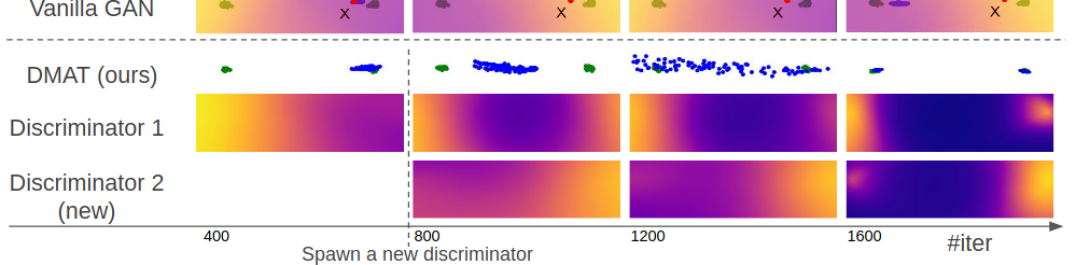
Figure 1: Visualizing training trajectories: Distribution of real (green dots) and fake (blue dots) over the course of vanilla GAN (top row) and our method (the second row and below). The background color indicates the prediction heatmap of the discriminator with blue being fake and warm yellow being real. Once the vanilla GAN falls into mode collapse (top row), it ends up oscillating between the two modes without convergence. Also, the discriminator’s prediction at point X oscillates, indicating catastrophic forgetting in the discriminator. AMAT algorithm adapts to the need, and a new discriminator is spawned during training which effectively learns the forgotten mode, guiding the GAN optimization toward convergence.

2 Related Works

Previous works have focused on independently solving either catastrophic forgetting in supervised learning or mode collapse during GAN training. In this section we review these works in detail and discuss our commonalities and differences.

2.1 Mitigating Mode Collapse in GANs

Along with advancement in the perceptual quality of images generated by GAN (Miyato et al., 2018; Karras et al., 2019; Brock et al., 2018; Karras et al., 2020), a large number of papers (Durugkar et al., 2016; Metz et al., 2016; Arjovsky et al., 2017; Srivastava et al., 2017; Nguyen et al., 2017; Lin et al., 2018; Mescheder et al., 2018; Karras et al., 2019) identify the problem of mode collapse in GANs and aim to mitigate it. However mode collapse was seen as a secondary symptom that would be naturally solved as the stability of GAN optimization progresses (Arjovsky et al., 2017; Mescheder et al., 2018; Bau et al., 2019). To explicitly address mode collapse, Unrolled GAN (Metz et al., 2016) proposes an unrolled optimization of the discriminator to optimally match the generator objective, thus preventing mode collapse. VEEGAN (Srivastava et al., 2017) utilizes the reconstruction loss on the latent space. PacGAN (Lin et al., 2018) feeds multiple samples of the same class to the discriminator when making the decisions about real/fake. In contrast, our approach can be plugged into existing state-of-the-art GAN frameworks to yield additional performance boost.

2.2 Multi-adversarial Approaches

The idea of employing more than one adversarial network in GANs to improve results has been explored by several previous works independent of the connection to continual learning and catastrophic forgetting. MGAN (Hoang et al., 2018) uses multiple generators, while D2GAN (Nguyen et al., 2017) uses two discriminators, and GMAN (Durugkar et al., 2016) and MicrobatchGAN (Mordido et al., 2020) proposed a method with more than two discriminators that can be specified as a training hyperparameter beforehand. However, all previous works require the number of discriminators to be fixed beforehand, which is a major drawback since it depends on several intricate factors such as training dynamics, data distribution complexity, model architecture, initialization hyper-parameters etc. and is expensive and difficult to approximate even with several runs of the algorithm. In contrast, noting by the connection of multi-adversarial training to parameter expansion approaches to catastrophic forgetting, we propose an adaptive method that can add discriminators incrementally during training thus achieving superior performance than existing works both on data quality metrics as well as overall computational effort.

$g(\mathbf{z})=$	${1}$	$\mathbf{A}_{392\times 2}$	$\mathbf{z}$	MLP	MLP, $\mathbf{A}_{392\times 2}$	MNIST
Label	Level I	Level II	Level III	Level IV	Level V	-
GAN-NS (Goodfellow et al., 2014)	✕ | ✓	✕ | ✓	✕ | ✕	✕ | ✕	✕ | ✕	✓
WGAN (Arjovsky et al., 2017)	✓ | ✓	✕ | ✓	✕ | ✓	✕ | ✕	✕ | ✕	✓
Unrolled GAN (Metz et al., 2016)	✓ | ✓	✓ | ✓	✓ | ✓	✓ | ✓	✕ | ✕	✓
D2GAN (Nguyen et al., 2017)	✓ | ✓	✓ | ✓	✓ | ✓	✓ | ✓	✕ | ✕	✓
GAN-NS + AMAT	✓ | ✓	✓ | ✓	✓ | ✓	✓ | ✓	✕ | ✕	✓

Table 1: ✓  indicates that the generator could effectively learn all the data modes, while ✕  means despite best efforts with tuning the training suffers from mode collapse (more than a quarter of data modes dropped). We show results with the SGD (left) & ADAM (right) optimizers. MNIST results with ADAM optimizer are provided for reference. We observe that MNIST is a relatively easy dataset, falling between Level I and II in terms of complexity.

2.3 Overcoming Catastrophic Forgetting in GAN

Methods to mitigate catastrophic forgetting can be categorized into three groups: a) regularization based methods (Kirkpatrick et al., 2017) b) memory replay based methods (Rebuffi et al., 2017) c) network expansion based methods (Zhang et al., 2018; Rajasegaran et al., 2019). Our work is closely related to the third category of methods, which dynamically adds more capacity to the network, when faced with novel tasks. This type of methods, adds plasticity to the network from new weights (fast-weights) while keeping the stability of the network by freezing the past-weights (slow-weights). Additionally, we enforce stability by letting a discriminator to focus on a few set of classes, not by freezing its weights.

The issue of catastrophic forgetting in GANs has been sparsely explored before. Chen et al. (2018) and Tran et al. (2019) propose a self-supervised learning objective to prevent catastrophic forgetting by adding new loss terms. Liang et al. (2018) proposes an online EWC based solution to tackle catastrophic forgetting in the discriminator. We propose a prominently different approach based on parameter expansion rather than regularization. While the regularization based approaches such as Liang et al. (2018) attempt to retain the previously learnt knowledge by constrained weight updates, the parameter expansion approaches effectively sidestep catastrophic forgetting by freezing previously encoded knowledge. Thanh-Tung and Tran (2020) also discuss the possibility of catastrophic forgetting in GAN training but their solution is limited to theoretical analyses with simplistic proposals such as assigning larger weights to real samples and optimizing the GAN objective with momentum. Practically, we observed that their method performs worse than a plain vanilla DCGAN on simple real world datasets like CIFAR10. In contrast, our method leverages insights from continual learning and has a direct connections to prevalent parameter expansion approaches in supervised learning. We benchmark extensively on several datasets and state-of-the-art GAN approaches where our method consistently achieves superior results to the existing methods.

3 Proposed Method

In this section, we first describe our proposed data generation procedure that we use as a petri dish for studying mode collapse in GANs. The procedure uses random normalizing flows for simultaneously allowing training on complex high dimensional distributions yet being perfectly amenable to 2D visualizations. Next, we describe our proposed Adaptive Multi Adversarial Training (AMAT) algorithm that effectively detects catastrophic forgetting and spawns a new discriminator to prevent mode collapse.

3.1 Synthetic Data Generation with Normalizing flows

Mode dropping in GANs in the context of catastrophic forgetting of the discriminator is a difficult problem to investigate using real datasets. This is because the number of classes in the dataset cannot be easily increased, the classes of fake samples are often ambiguous, and the predictions of the discriminator cannot be easily visualized across the whole input space. In this regard, we present a simple yet powerful data synthesis procedure that can generate complex high dimensional multi-modal distributions, yet maintaining perfect 2-D visualization capabilities. Samples from a 2-D Gaussian distribution are augmented with biases and subjected to an invertible normalizing flow (Karami et al., 2019) parameterized by well conditioned functions $g_{i}:\mathbb{R}^{d^{0}_{i}}\rightarrow\mathbb{R}^{d^{1}_{i}}$. This function can be followed by a linear upsampling transformation parameterized by a $d^{1}_{i}\times d^{0}_{i+1}$ dimensional matrix $A^{i}$ (Algorithm 1). The entire transform is deliberately constructed to be a bijective function so that every generated sample in $\hat{y}\in\mathbb{R}^{D}$ can be analytically mapped to $\mathbb{R}^{2}$, allowing perfect visualization on 2D space. Furthermore, by evaluating a dense grid of points in $\mathbb{R}^{2}$, we can understand discriminator’s learned probability distribution on $\mathbf{z}$ manifold as a heatmap on the 2D plane. This synthetic data generation procedure enables studying mode collapse in a controlled setting. This also gives practitioners the capability to train models on a chosen data complexity with clean two-dimensional visualizations of both the generated data and the discriminator’s learnt distribution. This tool can be used for debugging new algorithms using insights from the visualizations. In the case of mode collapse, a quick visual inspection would give the details of which modes face mode collapse or get dropped from discriminator’s learnt distribution.

3.2 Adaptive Multi Adversarial Training

Building upon the insight on relating catastrophic forgetting in discriminator to mode collapse in generator, we propose a multi adversarial generative adversarial network training procedure. The key intuition is that the interplay of catastrophic forgetting in the discriminator with the GAN minimax game, leads to an oscillation generator. Thus, as the generator shifts to a new set of modes the discriminator forgets the learnt features on the previous modes.   Input: Mean $\{\mu_{i}\}_{i=1}^{K}$ and standard deviation $\{\sigma_{i}\}_{i=1}^{K}$ for initialization, $\{g_{i}\}_{i=1}^{L}$ well conditioned $\mathbb{R}^{2}\rightarrow\mathbb{R}^{2}$ functions   Sample weights ${\bm{w}}\sim\text{Dirichlet}(K)$ /* Sample from 2D gaussian mixture */   $\mathbf{x}_{2D}\sim\Sigma_{i=1}^{N}w_{i}\mathcal{N}(\mu_{i},\sigma_{i})$   $\mathbf{x}^{0}_{2D}=\Big{[}[x^{0}_{2D};{1}],[x^{1}_{2D};{1}]\Big{]}$
 /* Randomly Init Normalizing Flow */   for $k=1$ to $k=K$ do      if k is even then         ${\bm{x}}^{k}=\big{[}{\bm{x}}^{k}_{0},{\bm{x}}^{k}_{1}\cdot g_{k}({\bm{x}}^{k}_{0})\big{]}$      else         ${\bm{x}}^{k}=\big{[}{\bm{x}}^{k}_{0}\cdot g_{k}({\bm{x}}^{k}_{1}),{\bm{x}}^{k}_{1}\big{]}$      end if   end for Algorithm 1 Synthetic Data Generation Algorithm 2 DSPAWN: Discriminator Spawning Routine   Require: Exemplar Data $\{{\bm{e}}\}_{i=1}^{m}$   Input: Discriminator set $\displaystyle{\mathbb{D}}=\{f_{w}^{i}\}_{i=1}^{K}$
 /* Check forgetting on exemplars */   for $i=1$ to $i=m$ do      ${\bm{s}}[k]\leftarrow f_{w}^{k}({\bm{e}}_{i})\ \forall\ k\ \in\{1\dots K\}$       if  $K*\max({\bm{s}})>\alpha_{t}*\sum_{k}{\bm{s}}[k]$ then         Initialize $f_{w}^{K+1}$ with random weights $w$
 /* Spawn a new discriminator */         Initialize random weight $w^{K+1}$         $\displaystyle{\mathbb{D}}\leftarrow\{f_{w}^{i}\}_{i=1}^{K}\bigcup f_{w}^{K+1}$         break      end if   end for   return Discriminator Set $\displaystyle{\mathbb{D}}$ Algorithm 3 A-MAT: Adaptive Multi-Adversarial Training   Require: ${\bm{w}}^{i}_{0}$, ${\bm{\theta}}_{0}$ initial discriminator & generator params, greediness param $\epsilon$, $\{T_{k}\}$ spawn warmup iteration schedule   $\displaystyle{\mathbb{D}}\leftarrow\{f_{w}^{0}\}$    while ${\bm{\theta}}$ has not converged do      Sample $\{{\bm{z}}^{(i)}\}_{i=1}^{B}\sim p(z)$      Sample $\{{\bm{x}}^{(i)}\}_{i=1}^{B}\sim\mathbb{P}_{r}$      Sample $\{\sigma_{1}(i)\}_{i=1}^{B}\sim\text{Uniform}(1,K)$      Sample $\{\alpha(i)\}_{i=1}^{B}\sim\text{Bernoulli}(\epsilon)$
/* Loss weights over discriminators */      Sample weights ${\bm{m}}\sim\text{Dirichlet}(K)$      $\hat{\bm{x}}^{(i)}\leftarrow g_{\theta}({\bm{z}}^{(i)})$      $\sigma_{2}(i)\leftarrow\operatorname*{arg\,min}_{k}f_{w}^{k}(\hat{\bm{x}}^{(i)})$
 /* Discriminator responsible for $\hat{x}^{(i)}$ */      $\sigma_{z}(i)\leftarrow\alpha(i)\sigma_{1}(i)+(1-\alpha(i))\sigma_{2}(i)$
 /* Discriminator responsible for $x^{(i)}$ */      $\sigma_{x}(i)\leftarrow\sigma_{1}(i)$
 /* Training Discriminators */ $L_{w}\leftarrow\sum_{i=1}^{B}[f_{w}^{\sigma_{x}(i)}({\bm{x}}_{i})-1]^{-}-[f_{w}^{\sigma_{z}(i)}(\hat{\bm{x}}_{i})+1]^{+}$      for $k=1$ to $k=|\displaystyle{\mathbb{D}}|$ do         $w^{k}\leftarrow\text{ADAM}(L_{w})$      end for
 /* Training Generator */      $s[k]\leftarrow\sum_{i=1}^{B}f_{w}^{k}(\hat{\bm{x}}^{(i)})\ \forall\ k\ \in\{1\dots|\displaystyle{\mathbb{D}}|\}$
 /* Weighed mean over discriminators */      $L_{\theta}\leftarrow\text{sort}({\bm{m}})\cdot\text{sort}(s)$      $\theta\leftarrow\text{ADAM}(L_{\theta})$       if more than $T_{t}$ warm-up iterations since the last spawn then         $\displaystyle{\mathbb{D}}\leftarrow\text{DSPAWN}(\{f_{w}^{i}\})$      end if   end while However if there are multiple discriminators available, each discriminator can implicitly specialize on a subset of modes. Thus even if the generator oscillates, each discriminator can remember their own set of modes, and they will not need to move to different set of modes. This way we can effectively sidestep forgetting and ensure the networks do not face significant distribution shift. A detailed version of our proposed method is presented in Algorithm 3.

Spawning new discriminators: We initialize the AMAT training Algorithm 3 with a regular GAN using just one discriminator. We also sample a few randomly chosen exemplar data points with a maximum of one real sample per mode, depending on dataset complexity. The exemplar data points are used to detect the presence of catastrophic forgetting in the currently active set of discriminators $\displaystyle{\mathbb{D}}$ and spawn a new discriminator if needed. Specifically (Algorithm 2), we propose that if any discriminator among $\displaystyle{\mathbb{D}}$ has an unusually high score over an exemplar data point ${\bm{e}}_{i}$, this is because the mode corresponding to ${\bm{e}}_{i}$ has either very poor generated samples or has been entirely dropped.

In such a situation, if training were to continue we risk catastrophic forgetting in the active set $\displaystyle{\mathbb{D}}$, if the generator oscillate to near ${\bm{e}}_{i}$. This is implemented by comparing the $\max$ score over $\displaystyle sD$ at ${\bm{e}}_{i}$ to the average score over $\displaystyle{\mathbb{D}}$ and spawning a new discriminator when the ratio exceeds $\alpha_{t}(>1)$. Further, we propose to have $\alpha_{t}(>1)$ a monotonically increasing function of $|\displaystyle{\mathbb{D}}|$, thus successively making it harder to spawn each new discriminator. Additionally, we use a warm-up period $T_{t}$ after spawning each new discriminator from scratch to let the spawned discriminator train before starting the check over exemplar data-points.

Multi-Discriminator Training: We evaluate all discriminators in $\displaystyle{\mathbb{D}}$ on the fake samples but do not update all of them for all the samples. Instead, we use the discriminator scores to assign responsibility of each data point to only one discriminator.

Training over fake samples: We use an $\epsilon$-greedy approach for fake samples where the discriminator with the lowest output score is assigned responsibility with a probability $1-\epsilon$ and a random discriminator is chosen with probability $\epsilon$.

Training over real samples: The discriminator is always chosen uniformly randomly thus we slightly prefer to assign the same discriminator to the fake datapoints from around the same mode to ensure that they do not forget the already learnt modes and switch to another mode. The random assignment of real points ensure that the same preferentially treated discriminator also gets updated on real samples.

Further for optimization stability, we ensure that the real and fake sample loss incurred by each discriminator is roughly equal in each back-propagation step by dynamically reweighing them by the number of data points the discriminator is responsible for. We only update the discriminator on the losses of the samples they are responsible for. While it may seem that adding multiple discriminators makes the procedure expensive, in practice the total number of added discriminator networks never surpass three for the best results. It is possible to change the hyperparameters to allow a large number of discriminators but that results in sub-optimal results and incomplete training. The optimal hyperparameter selection is explained in the Appendix for each dataset. Further, the additional discriminators get added during later training stages and are not trained from the start, saving compute in comparison to prior multi-adversarial works which train all the networks from the beginning. Also, unlike AdaGAN (Tolstikhin et al., 2017) and similar Boosted GAN models that need to store multiple Generators post training, the final number of parameters required during inference remains unchanged under AMAT . Thus the inference time remains the same, but with enhanced mode coverage and sample diversity. Unlike (Tolstikhin et al., 2017), our discriminator addition is adaptive, i.e. discriminators are added during the training thus being more efficient.

Generator Training: We take a weighted mean over the discriminators scores on the fake datapoints for calculating the generator loss. At each step, the weights each discriminator in $\displaystyle{\mathbb{D}}$ gets is in decreasing order of its score on the fake sample. Hence, the discriminator with the lowest score is given the most weight since it is the one that is currently specializing on the mode the fake sample is related to. In practice, we sample weights randomly from a Dirichlet distribution (and hence implicitly they sum to $1$) and sort according to discriminator scores to achieve this. We choose soft weighing over hard binary weights because since the discriminators are updated in an $\epsilon$ greedy fashion, the discriminators other than the one with the best judgment on the fake sample might also hold useful information. Further, we choose the weights randomly instead of fixing a chosen set to ensure AMAT is more deadset agnostic since the number of discriminator used changes with the dataset complexity so does the number of weights needed. While a suitable function for generating weights can work well on a particular dataset, we found random weights to work as well across different settings.

4 Results

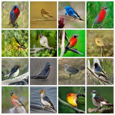
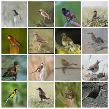
Figure 3: Sample Diversity on CUB200: We showcase samples from a BigGAN pretrained on imagenet & finetuned on CUB200 with the AMAT procedure (left) and from an identical BigGAN finetuned without AMAT (right). Observe that while the sample quality is good for both, the samples generated with AMAT are more colorful & diverse, with bright reds and yellow against several backgrounds. While the samples from vanilla fine-tuning are restricted to whites/grays & only a hint of color.

We test our proposed method on several synthetic and real datasets & report a consistent increase in performance on GAN evaluation metrics such as Inception Score (Salimans et al., 2016) and Frechét Inception Distance (Heusel et al., 2017) with our proposed AMAT. We also showcase our performance in the GAN fine-tuning regime with samples on the CUB200 dataset (Welinder et al., 2010) which qualitatively are more colorful and diverse than an identical BigGAN without AMAT (Figure 3).

	GAN	UnrolledGAN	D2GAN	RegGAN	DCGAN	with AMAT
# Modes covered	$628.0\pm 140.9$	$817.4\pm 37.9$	$1000\pm 0.0$	$955.5\pm 18.7$	$849.6\pm 62.7$	$\mathbf{1000\pm 0.0}$
KL (samples $\|$ data)	$2.58\pm 0.75$	$1.43\pm 0.12$	$0.080\pm 0.01$	$0.64\pm 0.05$	$0.73\pm 0.09$	$0.078\pm 0.01$

Table 2: Quantitative Results on the Stacked MNIST dataset: Applying our proposed adaptive multi adversarial training (AMAT) procedure to a simple DCGAN achieves perfect mode coverage, better than many existing methods for mode collapse.

			GAN-NS	AMAT +		AMAT +
Model	D2GAN	MicrobatchGAN	w/ ResNet	GAN-NS	DCGAN	DCGAN
IS	$7.15\pm 0.07$	$6.77$	$6.7\pm 0.06$	$\mathbf{8.1\pm 0.04}$	$6.03\pm 0.05$	$\mathbf{6.32\pm 0.06}$
FID	-	-	$28.91$	$\mathbf{16.35}$	$33.42$	$\mathbf{30.14}$
	WGAN-GP	AMAT +		AMAT +		AMAT +
Model	w/ ResNet	WGAN-GP	SN-GAN	SN-GAN	BigGAN	BigGAN
IS	$7.59\pm 0.10$	$\mathbf{7.80\pm 0.07}$	$8.22\pm 0.05$	$\mathbf{8.34\pm 0.04}$	$9.22$	$\mathbf{9.51\pm 0.06}$
FID	$19.2$	$\mathbf{17.2}$	$14.21$	$\mathbf{13.8}$	$8.94$	$\mathbf{6.11}$

Table 3: Quantitative Results on CIFAR10: We benchmark AMAT against several other multi-adversarial baselines as well as on several GAN architectures across all of which we observe a consistent performance increase.

4.1 Synthetic Data

We utilize the proposed synthetic data generation procedure with randomly initialized normalizing flows to visualize the training process of a simple DCGAN (Radford et al., 2015). Figure 1 visualizes such a training process for a simple bimodal distribution. Observing the pattern of generated samples over the training iteration and the shifting discriminator landscape, we note a clear mode oscillation issue present in the generated samples driven by the shifting discriminator output distribution. Focusing on a single fixed real point in space at any of the modes, we see a clear oscillation in the discriminator output probabilities strongly indicating the presence of catastrophic forgetting in the discriminator network.

Effect of Data Complexity on Mode Collapse: We use the flexibility in choosing transformations $g_{i}$ to generate datasets of various data distribution complexities as presented in Table 1. Choosing $g(z)$ with successively more complicated transformations can produce synthetic datasets of increasing complexity, the first five of which we roughly classify as Levels. The Levels are generated by using simple transforms such as identitym constant mapping, small Multi layer perceptrons and well conditioned linear transforms ($\mathbf{A}$).

On this benchmark, we investigate mode collapse across different optimizers such as SGD & ADAM (Kingma and Ba, 2014) on several popular GAN variants such as the non-saturating GAN Loss (GAN-NS) (Goodfellow et al., 2014), WGAN (Arjovsky et al., 2017) and also methods targeting mitigating mode collapse specifically such as Unrolled GAN (Metz et al., 2016) and D2GAN (Nguyen et al., 2017). We show results of our proposed AMAT training procedure with a simple GAN-NS, which matches performance with other more complicated mode collapse specific GAN architectures, all of which are robust to mode collapse up to Level IV. In practice we find all benchmarked methods to collapse at Level V. Thus, in contrast to other simple datasets like MNIST (LeCun, 1998), Gaussian ring, or Stacked MNIST (Metz et al., 2016), the complexity of our synthetic dataset can be arbitrarily tuned up or down to gain insight into the training and debugging of GAN via visualizations.

Effect	Large $|\displaystyle{\mathbb{D}}|$	Spawn too late	Greedy $\displaystyle\nabla$D	Random for fake	$\mathbf{1}$-hot weight	Proposed
Ablation	Small $\alpha$, Short $T_{t}$	Long $T_{t}$ schedule	$\epsilon=0$	$\epsilon$-greedy for real	vector ${\bm{m}}$	Method
IS	$8.83\pm 0.04$	$9.28\pm 0.08$	$9.31\pm 0.06$	$8.95\pm 0.04$	$9.25\pm 0.05$	$9.51\pm 0.06$
FID	$14.23$	$9.37$	$8.6$	$12.5$	$9.25$	$6.11$

Table 4: BigGAN + AMAT Ablations on CIFAR10 (A) A spawning condition with small $\alpha$ and short warmup schedule that leads to large number of discriminators (>$7$) (B) Long warm-up schedules that spawn new discriminators late into training (C) A greedy strategy for assigning responsibility of fake samples ($\epsilon=0$) (D) Flipping the data splitting logic with responsibilities of fake samples being random and of real being $\epsilon$-greedy (E) Choosing the discriminator with lowest score for updating Generator instead of soft random weighting.

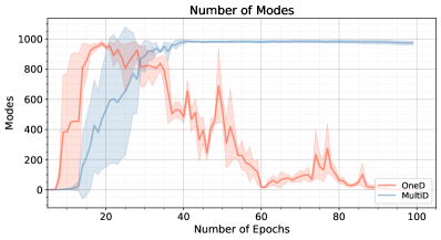
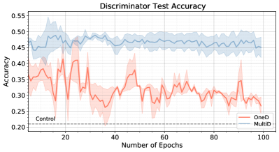
Figure 2: Investigating the forgetting-collapse interplay: We investigate our hypothesis that catastrophic forgetting is associated with mode collapse. On the left pane, we plot the magnitude of mode collapse by counting the number of modes produced by the generator. On the right pane, we assess the quality of the discriminator features by plotting the accuracy of linear classifier on top of the discriminator features at each epoch. In the original model, the coverage of modes and the quality of discriminator features are both low and decreasing. In particular, the test accuracy from the discriminator’s features drops almost to randomly initialized weights (shown as control). On the other hand, adding AMAT (MultiD) dramatically improves both mode coverage and the discriminator test accuracy.

4.2 Stacked MNIST

We also benchmark several models on the Stacked MNIST dataset following (Metz et al., 2016; Srivastava et al., 2017). Stacked MNIST is an extension of the popular MNIST dataset (LeCun et al., 1998) where each image is expanded in the channel dimension to $28\times 28\times 3$ by concatenating $3$ single channel images. The resulting dataset has a $1000$ overall modes. We measure the number of modes covered by the generator as the number of classes that are generated at least once within a pool of $25,600$ sampled images. The class of the generated sample is identified with a pretrained MNIST classifier operating channel wise on the original stacked MNIST image.

Understanding the forgetting-collapse interplay: In Section 1, we discuss our motivation for studying catastrophic forgetting for mitigating mode collapse. We also design an investigative experiment to explicitly observe this interplay by comparing the number of modes the generator learns against the quality of features the discriminator learns throughout GAN training on the stacked MNIST dataset. We measure the number of modes captured by the generator through a pre-trained classification network trained in a supervised learning fashion and frozen throughout GAN training. To measure the amount of ‘forgetting‘ in discriminator, we extract features of real samples from the penultimate layer of the discriminator and train a small classifier on the real features for detecting real data mode. This implicitly indicates the quality and information contained in the the discriminator extracted features. However, the performance of classification network on top of discriminator features is confounded by the capacity of the classification network itself. Hence we do a control experiment, where we train the same classifier on features extracted from a randomly initialized discriminator, hence fixing a lower-bound to the classifier accuracy.

Classes	Plane	Car	Bird	Cat	Deer	Dog	Frog	Horse	Ship	Truck	Avg
BigGAN	$24.23$	$12.32$	$24.85$	$21.21$	$12.81$	$22.74$	$17.95$	$13.16$	$12.11$	$18.39$	$8.94$
$+$ AMAT	$20.50$	$10.30$	$23.48$	$18.48$	$11.51$	$19.41$	$11.50$	$12.24$	$10.69$	$12.94$	$6.11$
$\Delta\%$	$18.2$	$19.6$	$5.8$	$14.8$	$11.3$	$17.2$	$\mathbf{56.1}$	$7.5$	$11.7$	$\mathbf{42.1}$	$\mathbf{46.3}$

Table 5: Per-class FID on CIFAR10: FID improves consistently across all classes.

Referring to Figure 2, we observe a clear relation between the number of modes the generator covers at an iteration and the accuracy of the classification network trained on the discriminator features at the same iteration. In the vanilla single discriminator scenario, the classification accuracy drops significantly, indicating a direct degradation of the discriminative features which is followed by a complete collapse of G. In the collapse phase, the discriminator’s learnt features are close to random with the classification accuracy being close to that of the control experiment. This indicates the presence of significant catastrophic forgetting in the the discriminator network.

In contrast, training the same generator with the proposed AMAT procedure leads to stable training with almost all the modes being covered. The classification accuracy increasing before saturation. Catastrophic forgetting is effectively sidestepped by adaptive multi adversarial training which produces stable discriminative features during training that provide a consistent training signal to the generator thereby covering all the modes with little degradation.

4.3 CIFAR10

We extensively benchmark AMAT on several GAN variants including unconditional methods such as DCGAN (Radford et al., 2015), ResNet-WGAN-GP (Gulrajani et al., 2017; He et al., 2016) & SNGAN (Miyato et al., 2018) and also conditional models such as BigGAN (Brock et al., 2018). Table 3 shows the performance gain on standard GAN evaluation metrics such as Inception Score and Fréchet distance of several architectures when trained with AMAT procedure. The performance gains indicate effective curbing of catastrophic forgetting in the discriminator with multi adversarial training. We use the public evaluation code from SNGAN (Miyato et al., 2018) for evaluation. Despite having components such as spectral normalization, diversity promoting loss functions, additional R1 losses & other stable training tricks that might affect catastrophic forgetting to different extents, we observe a consistent increase in performance across all models. Notably the ResNet GAN benefits greatly with AMAT despite a powerful backbone – with IS improving from $6.7$ to $8.1$, indicating that the mode oscillation problem is not mitigated by simply using a better model.

AMAT improves performance by over $35\%$ even on a well performing baseline such as BigGAN (Table 3). We investigate classwise FID scores of a vanilla BigGAN and an identical BigGAN + AMAT on CIFAR10 and report the results in Table 5. Performance improves across all classes with previously poor performing classes such as ‘Frog’ & ‘Truck’ experiencing the most gains. Further, we ablate several key components of AMAT procedure on the BigGAN architecture with results reported in Table 4. We observe all elements to be critical to overall performance. Specifically, having a moderate $\alpha$ schedule to avoid adding too many discriminators is critical. Another viable design choice is to effectively flip the algorithm’s logic and instead choose the fake points randomly while being $\epsilon$ greedy on the real points. This strategy performs well on simple datasets but loses performance with BigGAN on CIFAR10 (Table 4). In all experiments, the computational time during inference is the same as the base model, irrespective of the number of discriminators added during the training, since only a single generator is trained with AMAT and all the discriminators are discarded.

5 Conclusion

In summary, motivated from the observation of catastrophic forgetting in the discriminator, we propose a new adaptive GAN training framework that adds additional discriminators to prevent mode collapse. We show that our method can be added to existing GAN frameworks to prevent mode collapse, generate more diverse samples and improve FID & IS. In future, we plan to apply AMAT to fight mode collapse in high resolution image generation settings.

Acknowledgements

We thank Jathushan Rajasegaran for his helping with the forgetting-collapse interplay experiments and Taesung Park for feedback and comments on the early drafts of this paper.

Appendix

CIFAR10 Experiments

BigGAN + AMAT Experiments

For the baseline we use the author’s official PyTorch implementation . For our experiments on AMAT $+$ BigGAN, we kept the optimizer as Adam (Kingma and Ba, 2014) and used the hyperparameters $\beta_{1}=0.0,\beta_{2}=0.9$. We did not change the model architecture parameters in any way. The best performance was achieved with learning rate $=0.0002$ for both the Generator and all the Discriminators. The batch size for the $G$ and all $D$ is $50$, and the latent dimension is chosen as $128$. The initial value of $T_{t}=5$ epochs, and after the first discriminator is added, $T_{t}$ is increased by 5 epochs every $T_{t}$ epochs. The initial value of $\alpha_{t}=1.5$, and it is increased by a factor of $3.5$ every time a discriminator is added. To check whether to add another discriminator or not, we use 10 exemplar images, 1 from each CIFAR10 class. While assigning datapoints to each discriminator, we use an epsilon greedy approach. We chose $\epsilon=0.25$, where the datapoint is assigned to a random discriminator with a probability $\epsilon$. The number of discriminator(s) updates per generator update is fixed at $4$. We also use exponential moving average for the generator weights with a decay of $0.9999$.

SN-GAN + AMAT Experiments

We used the SN-GAN implementation from https://github.com/GongXinyuu/sngan.pytorch, which is the PyTorch version of the authors’ Chainer implementation https://github.com/pfnet-research/sngan_projection. We kept the optimiser as Adam and used the hyperparameters $\beta_{1}=0.0,\beta_{2}=0.9$. The batch size for generator is $128$ and for the discriminators is $64$, and the latent dimension is $128$. The initial learning rate is $0.0002$ for both generator and the discriminators. The number of discriminator(s) updates per generator update is fixed at $7$. The initial value of $T_{t}=2$ epochs, and is increased by $1$ epoch after every discriminator is added. $\alpha_{t}$ is initialized as $1.5$, and is increased by a factor of $1.3$ after a discriminator is added, till $20$ epochs, after which it is increased by a factor of $3.0$. These larger increases in $\alpha_{t}$ are required to prevent too many discriminators from being added over all iterations. We chose $\epsilon=0.3$, where the datapoint is assigned to a random discriminator with a probability $\epsilon$. We use 10 exemplar images, 1 from each CIFAR10 class.

ResNet GAN: We use the same ResNet architecture as above, but remove the spectral normalization from the model. The optimizer parameters, learning rate and batch sizes remain the same as well. The number of discriminator(s) updates per generator update is fixed at $5$. The initial value of $T_{t}=10$ epochs, and is increased by $5$ epochs after every discriminator is added. $\alpha_{t}$ is initialized as $1.5$, and is increased by a factor of $2.0$ after a discriminator is added. We chose $\epsilon=0.2$, where the datapoint is assigned to a random discriminator with a probability $\epsilon$. We use 10 exemplar images, 1 from each CIFAR10 class.

ResNet WGAN-GP: In the above model, the hinge loss is replaced by the Wasserstein loss with gradient penalty. The optimizer parameters, learning rate and batch sizes remain the same as well.The number of discriminator(s) updates per generator update is fixed at $2$. The initial value of $T_{t}=5$ epochs, and is increased by $5$ epochs after a discriminator is added. $\alpha_{t}$ is initialized as $1.5$, and is increased by a factor of $3.0$ after a discriminator is added. We chose $\epsilon=0.2$, where the datapoint is assigned to a random discriminator with a probability $\epsilon$. We use 10 exemplar images, 1 from each CIFAR10 class. These images are chosen randomly from each class, and may not be the same as the ones for other CIFAR10 experiments.

DCGAN + AMAT Experiments

We used standard CNN models for our DCGAN as shown in Table 9. We use Adam optimizer with hyperparameters $\beta_{1}=0.0,\beta_{2}=0.9$. The learning rate for generator was $0.0002$, and the learning rate for the discriminator(s) was $0.0001$. The number of discriminators updates per generator was fixed at 1. The initial value of $T_{t}=4$ epochs, and is increased $5$ epochs after a discriminator is added. $\alpha_{t}$ is initialized as $1.5$ and is increased by a factor of $1.5$ every time a discriminator is added. We chose $\epsilon=0.3$, where the datapoint is assigned to a random discriminator with a probability $\epsilon$. We use 10 exemplar images, 1 from each CIFAR10 class.

Stacked MNIST Experiments

Stacked MNIST provides us a test-bed to measure mode collapse. A three channel image is generated by stacking randomly sampled MNIST classes, thus creating a data distribution if 1000 modes. We use this dataset to show that, when generator oscillates to a different set of modes, catastrophic forgetting is induced in discriminator and this prevents the generator to recover previous modes. To study this phenomenon, we need to measure the correlation between number of modes the generator covered and the catastrophic forgetting in the discriminator. Measuring the number of modes is straight forward, we can by simply classify each channels of the generated images using a MNIST pretrained classifier to find its corresponding mode. However, to measure catastrophic forgetting in the discriminator, we use a proxy setting, where we take the high-level features of the real images from the discriminator and train a simple classifier on top of that. The discriminative quality of the features taken from the discriminator indirectly measure the ability of the network to remember the modes. Finally, as a control experiment we randomize the weights of the discriminator, and train a classifiers on the feature taken from randomized discriminator. This is to show that, extra parameters in the classifier does not interfere our proxy measure for the catastrophic forgetting. Finally, we train a DCGAN with a single discriminator, and a similar DCGAN architecture with our proposed AMAT procedure, and measure the number of modes covered by the generator and the accuracy of the discriminator.

A Fair comparison on discriminator capacity

Our AMAT approach incrementally adds new discriminators to the GAN frameworks, and its overall capacity increases over time. Therefore, it is not fair to compare a model with AMAT training procedure with its corresponding the single discriminator model. As a fair comparison to our AMAT algorithm, we ran single discriminator model with approximately matching its discriminator capacity to the final AMAT model. For example, SN-GAN with AMAT learning scheme uses 4 discriminators at the end of its training. Therefore we use a discriminator with four times more parameters for the single discriminator SN-GAN model. This is done by increasing the convolutional fillters in the discriminator. Table 6 shows that, even after matching the network capacity, the single discriminator models do not perform well as compared to our AMAT learning.

	Scores	DCGAN	ResNetGAN	WGAN-GP	SN-GAN	BigGAN
	#of Param of D	1.10 M	3.22 M	2.06 M	4.20 M	8.42 M
w/o AMAT	IS	5.97 $\pm$ 0.08	6.59 $\pm$ 0.09	7.72 $\pm$ 0.06	8.24 $\pm$ 0.05	9.14 $\pm$ 0.05
	FID	34.7	36.4	19.1	14.5	10.5
	#of Param of D	1.02 M	3 $\times$ 1.05 M	2 $\times$ 1.05 M	4 $\times$ 1.05 M	8.50 M
+ AMAT	IS	6.32 $\pm$ 0.06	8.1 $\pm$ 0.04	7.80 $\pm$ 0.07	8.34 $\pm$ 0.04	9.51 $\pm$ 0.06
	FID	30.14	16.35	17.2	13.8	6.11

Table 6: Increasing network capacity alone does not capture more modes. Even after the discriminator capacity is matched, single discriminator GANs do not perform as well as multi-adversarial GANs with AMAT learning

Synthetic Data Experiments

We add flow-based non-linearity (Algorithm 1) to a synthetic 8-Gaussian ring dataset. We chose $K=5$ as our non-linearity depth and chose a randomly initiated 5 layer MLP as our non-linear functions. We use an MLP as our GAN generator and discriminator (Table 12). We use the Adam optimizer with hyperparameters $\beta_{1}=0.0,\beta_{2}=0.9$. The learning rate for the generator and discriminator was $0.0002$. The number of discriminator updates per generator update is fixed to 1, and the batch size is kept 64. The initial value of $T_{t}=5$ epochs, and is increased by $10$ every time a discriminator is added. $\alpha_{t}$ is initialized as $1.5$, and is increased by a factor of $1.5$ after a discriminator is added for the first 50 epochs. After that $\alpha_{t}$ is increased by a factor of $3$. We chose $\epsilon=0.25$, where the datapoint is assigned to a random discriminator with a probability $\epsilon$. 1 random datapoint from each of the 8 modes is selected as the exemplar image.

Figure 4 shows the difference in performance of a standard MLP GAN (12 and the same MLP GAN with AMAT. The GIF on the lefts shows a cyclic mode collapse due the discriminator suffering from catastrophic forgetting. The same GAN with is able to completely mitigate catastrophic forgetting with just 2 discriminators added during training, on a 728-dimensional synthetic data.

$z\in\mathbb{R}^{128}\sim\mathcal{N}(0,I)$
dense $\rightarrow 4\times 4\times 512$
$4\times 4$, stride$=$2 deconv. BN 256 ReLU
$4\times 4$, stride$=$2 deconv. BN 128 ReLU
$4\times 4$, stride$=$2 deconv. BN 64 ReLU
$3\times 3$, stride$=$1 conv. 3 Tanh

Table 7: *

Generator

$x\in\mathbb{R}^{32\times 32\times 3}$
$3\times 3$, stride$=$1 conv. 64 lReLU
$4\times 4$, stride$=$2 conv. 64 lReLU
$3\times 3$, stride$=$1 conv. 128 lReLU
$4\times 4$, stride$=$2 conv. 128 lReLU
$3\times 3$, stride$=$1 conv. 256 lReLU
$4\times 4$, stride$=$2 conv. 256 lReLU
$3\times 3$, stride$=$1 conv. 512 lReLU
dense $\rightarrow 1$

Table 8: *

Discriminator

Table 9: DCGAN Architecture for CIFAR10

$z\in\mathbb{R}^{25}\sim\mathcal{N}(0,I)$
dense $\rightarrow 128$, BN 128 ReLU
dense $\rightarrow 128$, BN 128 ReLU
dense $\rightarrow 512$, BN 512 ReLU
dense $\rightarrow 1024$, BN 1024 ReLU
dense $\rightarrow 2$, Tanh

Table 10: *

Generator

$x\in\mathbb{R}^{2}$
dense $\rightarrow 128$ ReLU
dense $\rightarrow 512$ ReLU
dense $\rightarrow 1$ Sigmoid

Table 11: *

Discriminator

Table 12: MLP architecture for Synthetic Dataset

Figure 4: GAN training visualization: (Figure contains animated graphics, better viewed in Adobe Acrobat Reader) Training trajectories of an MLP in table 12 (leftmost panel) and an MLP trained with our AMAT procedure (Algorithm 3) (rest three panels) on a $784$-dimensional synthetic dataset. Green dots represent real samples and the blue dots represent the generated samples. The vanilla GAN samples are overlayed against discriminator’s output heatmap where the warm yellow color indicates a high probability of being real and cold violet indicates fake. In the AMAT + GAN panels, the discriminator landscapes are shown separately for both discriminators with the second discriminator being spawned at iteration $4000$ (Algorithm 2). The $2$D visualizations of the $784$D data space is facilitated by our synthetic data generation procedure (Algorithm 1).

[loop,autoplay,width=0.24]5figs/gif0/047 [loop,autoplay,width=0.24]5figs/gen/frame_148 [loop,autoplay,width=0.24]5figs/d0/frame_148 [loop,autoplay,width=0.24]5figs/d1/frame_148

References

- Arjovsky et al. (2017) Martin Arjovsky, Soumith Chintala, and Léon Bottou. Wasserstein gan. arXiv preprint arXiv:1701.07875, 2017.
- Bau et al. (2019) David Bau, Jun-Yan Zhu, Jonas Wulff, William Peebles, Hendrik Strobelt, Bolei Zhou, and Antonio Torralba. Seeing what a gan cannot generate. In Proceedings of the International Conference Computer Vision (ICCV), 2019.
- Bousmalis et al. (2018) Konstantinos Bousmalis, Alex Irpan, Paul Wohlhart, Yunfei Bai, Matthew Kelcey, Mrinal Kalakrishnan, Laura Downs, Julian Ibarz, Peter Pastor, Kurt Konolige, et al. Using simulation and domain adaptation to improve efficiency of deep robotic grasping. In 2018 IEEE international conference on robotics and automation (ICRA), pages 4243–4250. IEEE, 2018.
- Brock et al. (2018) Andrew Brock, Jeff Donahue, and Karen Simonyan. Large scale gan training for high fidelity natural image synthesis. arXiv preprint arXiv:1809.11096, 2018.
- Chen et al. (2018) Ting Chen, Xiaohua Zhai, and Neil Houlsby. Self-supervised gan to counter forgetting. arXiv preprint arXiv:1810.11598, 2018.
- Durugkar et al. (2016) Ishan Durugkar, Ian Gemp, and Sridhar Mahadevan. Generative multi-adversarial networks. arXiv preprint arXiv:1611.01673, 2016.
- Fernando et al. (2017) Chrisantha Fernando, Dylan Banarse, Charles Blundell, Yori Zwols, David Ha, Andrei A Rusu, Alexander Pritzel, and Daan Wierstra. Pathnet: Evolution channels gradient descent in super neural networks. arXiv preprint arXiv:1701.08734, 2017.
- Goodfellow et al. (2014) Ian Goodfellow, Jean Pouget-Abadie, Mehdi Mirza, Bing Xu, David Warde-Farley, Sherjil Ozair, Aaron Courville, and Yoshua Bengio. Generative adversarial nets. In Advances in neural information processing systems, pages 2672–2680, 2014.
- Gulrajani et al. (2017) Ishaan Gulrajani, Faruk Ahmed, Martin Arjovsky, Vincent Dumoulin, and Aaron C Courville. Improved training of wasserstein gans. In Advances in neural information processing systems, pages 5767–5777, 2017.
- He et al. (2016) Kaiming He, Xiangyu Zhang, Shaoqing Ren, and Jian Sun. Deep residual learning for image recognition. In Proceedings of the IEEE conference on computer vision and pattern recognition, pages 770–778, 2016.
- Heusel et al. (2017) Martin Heusel, Hubert Ramsauer, Thomas Unterthiner, Bernhard Nessler, and Sepp Hochreiter. Gans trained by a two time-scale update rule converge to a local nash equilibrium. In Advances in neural information processing systems, pages 6626–6637, 2017.
- Hoang et al. (2018) Quan Hoang, Tu Dinh Nguyen, Trung Le, and Dinh Phung. Mgan: Training generative adversarial nets with multiple generators. In International Conference on Learning Representations, 2018.
- Hoffman et al. (2018) Judy Hoffman, Eric Tzeng, Taesung Park, Jun-Yan Zhu, Phillip Isola, Kate Saenko, Alexei Efros, and Trevor Darrell. Cycada: Cycle-consistent adversarial domain adaptation. In International conference on machine learning, pages 1989–1998. PMLR, 2018.
- Karami et al. (2019) Mahdi Karami, Dale Schuurmans, Jascha Sohl-Dickstein, Laurent Dinh, and Daniel Duckworth. Invertible convolutional flow. In Advances in Neural Information Processing Systems, pages 5635–5645, 2019.
- Karras et al. (2019) Tero Karras, Samuli Laine, and Timo Aila. A style-based generator architecture for generative adversarial networks. 2019.
- Karras et al. (2020) Tero Karras, Samuli Laine, Miika Aittala, Janne Hellsten, Jaakko Lehtinen, and Timo Aila. Analyzing and improving the image quality of stylegan. 2020.
- Kingma and Ba (2014) Diederik P Kingma and Jimmy Ba. Adam: A method for stochastic optimization. arXiv preprint arXiv:1412.6980, 2014.
- Kirkpatrick et al. (2017) James Kirkpatrick, Razvan Pascanu, Neil Rabinowitz, Joel Veness, Guillaume Desjardins, Andrei A Rusu, Kieran Milan, John Quan, Tiago Ramalho, Agnieszka Grabska-Barwinska, et al. Overcoming catastrophic forgetting in neural networks. Proceedings of the national academy of sciences, 114(13):3521–3526, 2017.
- LeCun (1998) Yann LeCun. The mnist database of handwritten digits. http://yann. lecun. com/exdb/mnist/, 1998.
- LeCun et al. (1998) Yann LeCun, Léon Bottou, Yoshua Bengio, and Patrick Haffner. Gradient-based learning applied to document recognition. Proceedings of the IEEE, 86(11):2278–2324, 1998.
- Liang et al. (2018) Kevin J Liang, Chunyuan Li, Guoyin Wang, and Lawrence Carin. Generative adversarial network training is a continual learning problem. arXiv preprint arXiv:1811.11083, 2018.
- Lin et al. (2018) Zinan Lin, Ashish Khetan, Giulia Fanti, and Sewoong Oh. Pacgan: The power of two samples in generative adversarial networks. In Advances in neural information processing systems, pages 1498–1507, 2018.
- McClelland et al. (1995) James L McClelland, Bruce L McNaughton, and Randall C O’Reilly. Why there are complementary learning systems in the hippocampus and neocortex: insights from the successes and failures of connectionist models of learning and memory. Psychological review, 102(3):419, 1995.
- McCloskey and Cohen (1989) Michael McCloskey and Neal J Cohen. Catastrophic interference in connectionist networks: The sequential learning problem. In Psychology of learning and motivation, volume 24, pages 109–165. Elsevier, 1989.
- Menon et al. (2020) Sachit Menon, Alexandru Damian, Shijia Hu, Nikhil Ravi, and Cynthia Rudin. Pulse: Self-supervised photo upsampling via latent space exploration of generative models. In Proceedings of the IEEE/CVF Conference on Computer Vision and Pattern Recognition (CVPR), June 2020.
- Mescheder et al. (2018) Lars Mescheder, Andreas Geiger, and Sebastian Nowozin. Which training methods for gans do actually converge? In International Conference on Machine learning (ICML), 2018.
- Metz et al. (2016) Luke Metz, Ben Poole, David Pfau, and Jascha Sohl-Dickstein. Unrolled generative adversarial networks. arXiv preprint arXiv:1611.02163, 2016.
- Miyato et al. (2018) Takeru Miyato, Toshiki Kataoka, Masanori Koyama, and Yuichi Yoshida. Spectral normalization for generative adversarial networks. arXiv preprint arXiv:1802.05957, 2018.
- Mordido et al. (2020) Gonçalo Mordido, Haojin Yang, and Christoph Meinel. microbatchgan: Stimulating diversity with multi-adversarial discrimination. arXiv preprint arXiv:2001.03376, 2020.
- Nguyen et al. (2017) Tu Nguyen, Trung Le, Hung Vu, and Dinh Phung. Dual discriminator generative adversarial nets. In Advances in Neural Information Processing Systems, pages 2670–2680, 2017.
- Nie et al. (2018) Dong Nie, Roger Trullo, Jun Lian, Li Wang, Caroline Petitjean, Su Ruan, Qian Wang, and Dinggang Shen. Medical image synthesis with deep convolutional adversarial networks. IEEE Transactions on Biomedical Engineering, 65(12):2720–2730, 2018.
- Radford et al. (2015) Alec Radford, Luke Metz, and Soumith Chintala. Unsupervised representation learning with deep convolutional generative adversarial networks. arXiv preprint arXiv:1511.06434, 2015.
- Rajasegaran et al. (2019) Jathushan Rajasegaran, Munawar Hayat, Salman H Khan, Fahad Shahbaz Khan, and Ling Shao. Random path selection for continual learning. In Advances in Neural Information Processing Systems 32, pages 12669–12679. Curran Associates, Inc., 2019.
- Rao et al. (2020) Kanishka Rao, Chris Harris, Alex Irpan, Sergey Levine, Julian Ibarz, and Mohi Khansari. Rl-cyclegan: Reinforcement learning aware simulation-to-real. In Proceedings of the IEEE/CVF Conference on Computer Vision and Pattern Recognition, pages 11157–11166, 2020.
- Ratcliff (1990) Roger Ratcliff. Connectionist models of recognition memory: constraints imposed by learning and forgetting functions. Psychological review, 97(2):285, 1990.
- Rebuffi et al. (2017) Sylvestre-Alvise Rebuffi, Alexander Kolesnikov, Georg Sperl, and Christoph H Lampert. icarl: Incremental classifier and representation learning. In Proceedings of the IEEE conference on Computer Vision and Pattern Recognition, pages 2001–2010, 2017.
- Rusu et al. (2016) Andrei A Rusu, Neil C Rabinowitz, Guillaume Desjardins, Hubert Soyer, James Kirkpatrick, Koray Kavukcuoglu, Razvan Pascanu, and Raia Hadsell. Progressive neural networks. arXiv preprint arXiv:1606.04671, 2016.
- Salimans et al. (2016) Tim Salimans, Ian Goodfellow, Wojciech Zaremba, Vicki Cheung, Alec Radford, and Xi Chen. Improved techniques for training gans, 2016.
- Srivastava et al. (2017) Akash Srivastava, Lazar Valkov, Chris Russell, Michael U Gutmann, and Charles Sutton. Veegan: Reducing mode collapse in gans using implicit variational learning. In Advances in Neural Information Processing Systems, pages 3308–3318, 2017.
- Thanh-Tung and Tran (2020) Hoang Thanh-Tung and Truyen Tran. On catastrophic forgetting and mode collapse in gans. arXiv preprint arXiv:1807.04015, 2020.
- Tolstikhin et al. (2017) Ilya O Tolstikhin, Sylvain Gelly, Olivier Bousquet, Carl-Johann Simon-Gabriel, and Bernhard Schölkopf. Adagan: Boosting generative models. In Advances in neural information processing systems, pages 5424–5433, 2017.
- Tran et al. (2019) Ngoc-Trung Tran, Viet-Hung Tran, Bao-Ngoc Nguyen, Linxiao Yang, et al. Self-supervised gan: Analysis and improvement with multi-class minimax game. In Advances in Neural Information Processing Systems, pages 13253–13264, 2019.
- Welinder et al. (2010) P. Welinder, S. Branson, T. Mita, C. Wah, F. Schroff, S. Belongie, and P. Perona. Caltech-UCSD Birds 200. Technical Report CNS-TR-2010-001, California Institute of Technology, 2010.
- Wolterink et al. (2017) Jelmer M Wolterink, Tim Leiner, Max A Viergever, and Ivana Išgum. Generative adversarial networks for noise reduction in low-dose ct. IEEE transactions on medical imaging, 36(12):2536–2545, 2017.
- Yi et al. (2019) Xin Yi, Ekta Walia, and Paul Babyn. Generative adversarial network in medical imaging: A review. Medical image analysis, 58:101552, 2019.
- Zhang et al. (2019) Jeffrey O. Zhang, Alexander Sax, Amir Zamir, Leonidas J. Guibas, and Jitendra Malik. Side-tuning: Network adaptation via additive side networks. 2019.
- Zhang et al. (2018) Mengshi Zhang, Yuqun Zhang, Lingming Zhang, Cong Liu, and Sarfraz Khurshid. Deeproad: Gan-based metamorphic testing and input validation framework for autonomous driving systems. In 2018 33rd IEEE/ACM International Conference on Automated Software Engineering (ASE), pages 132–142. IEEE, 2018.