Quantum kinetic theory for spin transport of quarks with background chromo-electromagnetic fields

Abstract

We derive the quantum kinetic equations for massive and massless quarks coupled with the background chromo-electromagnetic fields from the Wigner-function approach with the $\hbar$ expansion and effective power-counting scheme. For each case, one obtains coupled color-singlet and color-octet kinetic equations, which also involve the scalar and axial-vector components for the charge and spin transport. These kinetic equations delineate entangled evolution of the corresponding distribution functions decomposed in color space. At weak coupling, we derive the close form of the color-singlet kinetic equations for spin transport, which incorporates the diffusion term and the source term that triggers dynamical spin polarization led by correlation functions of color fields. Also, the non-dynamical source term is found in the axial Wigner function. The induced spin polarization and axial charge currents by these source terms are discussed under physical assumptions for color-field correlators in near-equilibrium quark gluon plasmas. In the constant-field limit, we further obtain non-vanishing axial Ward identities, from which we extract the pseudo-scalar condensate for massive quarks at finite temperature.

I Introduction

In recent years, there have been intensive studies on the developments and applications of quantum kinetic theory (QKT) for spin transport of relativistic fermions. In order to study non-equilibrium transport phenomena beyond e.g. the renown chiral magnetic effect (CME) Vilenkin (1980); Nielsen and Ninomiya (1983); Alekseev et al. (1998); Kharzeev (2006); Kharzeev et al. (2008); Fukushima et al. (2008) and chiral vortical effect (CVE) Vilenkin (1979); Erdmenger et al. (2009); Banerjee et al. (2011); Son and Surowka (2009); Landsteiner et al. (2011) in chiral matter composed of massless Weyl fermions, the chiral kinetic theory (CKT) as a QKT that captures the chiral anomaly Adler (1969); Bell and Jackiw (1969) and spin-orbit interaction could be constructed by introducing the Berry phase as quantum corrections from the adiabatic approximation Son and Yamamoto (2012); Stephanov and Yin (2012); Chen et al. (2014a, b, 2015). Alternatively, by employing the Wigner-function approach based on quantum field theories with the $\hbar$ expansion Gao et al. (2012); Chen et al. (2013); Son and Yamamoto (2013), the covariant CKT with systematic inclusions of both background electromagnetic fields and collisions involving quantum corrections has been later obtained Hidaka et al. (2017, 2018). There is a considerable number of related and follow-up work Manuel and Torres-Rincon (2014a, b); Hidaka and Yang (2018); Mueller and Venugopalan (2017, 2018); Huang et al. (2018); Yang (2018); Liu et al. (2019); Lin and Shukla (2019); Lin and Yang (2020); Shi et al. (2021); Fauth et al. (2021); Chen and Lin (2022); Luo and Gao (2021); Fang et al. (2022). In phenomenology, the CKT was broadly applied to relativistic heavy ion collisions Sun and Ko (2017, 2018); Liu et al. (2020a), Weyl semimetals Gorbar et al. (2017a, b, 2021), and neutrino transport in core-collapse supernovae Yamamoto and Yang (2020, 2021).

On the other hand, due to the observations of spin polarization of Lambda hyperons and spin alignments of vector mesons in heavy-ion experiments at RHIC and LHC Adamczyk et al. (2017); Adam et al. (2019); Acharya et al. (2020); Singha (2021) motivated by Refs. Liang and Wang (2005a, b); Becattini et al. (2013) in theory, further studies on the generalization of CKT to the QKT for massive fermions has been carried out in order to understand the dynamical spin polarization of strange quarks traveling through the quark gluon plasmas (QGP). In light of the Wigner-function approaches, such a collisionless QKT to track entangled spin and charge transport has been derived in Refs. Gao and Liang (2019); Weickgenannt et al. (2019); Hattori et al. (2019); Wang et al. (2019). Later, the systematic inclusion of collisions with quantum corrections was achieved by using the Kadanoff-Baym approach Yang et al. (2020); Sheng et al. (2021) and the extended phase space with non-local collisions Weickgenannt et al. (2021a, b). See also Refs. Florkowski et al. (2018); Zhang et al. (2019); Kapusta et al. (2020); Liu et al. (2020b); Li and Yee (2019); Wang et al. (2021); Wang and Zhuang (2021) for related studies of QKT and spin transport. In particular, from detailed balance of effective models, the vanishing collision term in QKT yields the Wigner function with vorticity correction that gives rise to spin polarization in global equilibrium Weickgenannt et al. (2021a); Wang et al. (2021). Such a result matches the one previously found from different methods Becattini et al. (2013); Fang et al. (2016) that provides the modified Cooper-Frye formula dictated by thermal vorticity, which successfully describes the global spin polarization observed by STAR collaboration after implementing numerical simulations Karpenko and Becattini (2017); Li et al. (2017); Xie et al. (2017); Wei et al. (2019); Ryu et al. (2021). In fact, the vanishing collision term of the CKT with Coulomb scattering yields the Wigner functions in local equilibrium, which incorporates extra corrections such as shear and chemical-potential gradient effects Hidaka et al. (2018). These corrections for massive fermions were later obtained by using the linear response theory Liu and Yin (2021a, b) and the statistical-field theory Becattini et al. (2021a) (see also Refs.Yi et al. (2021); Liu and Huang (2021)). Especially, the shear correction could lead to a substantial contributions on local spin polarization Fu et al. (2021); Becattini et al. (2021b); Yi et al. (2021); Florkowski et al. (2021); Yi et al. (2022); Sun et al. (2022), which is crucial to explain the experimental measurements Adam et al. (2019). However, it is also found that the local polarization is sensitive to the equation of state and freeze-out temperature Becattini et al. (2021b); Yi et al. (2021). Therefore, further studies involving non-equilibrium corrections from collisions are still required.

Nevertheless, the role of gluons or color degrees of freedom that may potentially affect the spin transport of quarks has been relatively overlooked in previous studies. Even though the thermalized gluons could lead to the spin diffusion through classical collisional effects shown in Refs. Li and Yee (2019); Yang et al. (2020), the quantum correction as a source term triggering the spin polarization from gluons is currently unknown. On the other hand, in addition to the scattering with on-shell gluons, there exist dynamically generated chromo-electromagnetic fields originating from Weibel-type instabilities in expanding QGP Mrowczynski (1988, 1993); Romatschke and Strickland (2003) that may potentially influence the spin transport of quarks in heavy ion collisions. Such color fields could result in anomalous dissipative transport that may dominate over the collisional effects in weakly coupled quantum chromodynamics (QCD) as proposed in Refs. Asakawa et al. (2006, 2007). See also Refs. Mrowczynski (2018); Carrington et al. (2020) for the analogous effect upon heavy-quark transport. The possible impact upon spin transport of quarks from color fields has been recently found by using a similar analysis Müller and Yang (2022), which in particular stems from the parity-odd correlators of color fields that could be potentially generated in different phases of heavy ion collisions from distinct mechanisms Joyce and Shaposhnikov (1997); Akamatsu and Yamamoto (2013); Mace et al. (2016); Tanji et al. (2016); Mace et al. (2020). In this paper, we present the derivation of QKT for massive quarks coupled with background color fields applied in Ref. Müller and Yang (2022) via the Wigner-function approach and effective power counting. More general results and details for the derivation of source terms in color-singlet Wigner functions and kinetic equations responsible for spin polarization are shown. Furthermore, we investigate the axial Ward identity from the axial charge current led by parity-odd color-field correlators in the constant-field limit. In addition, we perform a similar analysis for massless quarks by utilizing the CKT with background color fields constructed in Ref. Luo and Gao (2021).

Since the application of the derived QKT to QGP relies on several assumptions, here we briefly summarize the validity and critical approximations of our approach. Similar to the generic QKT with $\hbar$ expansion, it is required the energy of a quasi-particle is much larger than the gradient scale, $\epsilon_{\bm{p}}\gg\mathcal{O}(\partial)$. For the QKT of massive quarks derived in Sec. III, it is further subject to $m\gg\mathcal{O}(\partial)$ with $m$ being the quark mass due to a technical reason. Our approach is applicable to weakly coupled QCD and the collision term is assumed to be suppressed by sufficiently strong background color fields. Moreover, the other sources for spin polarization pertinent to the fluid properties such as thermal vorticity are assumed to be relatively small and thus neglected. In order to further solve for dynamical spin polarization from kinetic equations, we further assume the correlation function of color fields takes a Gaussian form depending on only the time difference in light of space-time translational invariance and propose a hierarchy for different color-field correlators according to the screening of chromo-electric fields.

This article is organized as follows: In Sec. II, we derive the master equations from free-streaming Kadanoff-Baym equation for massive quarks under background color fields. In Sec. III, we solve for the perturbative solution and kinetic equations up to $\mathcal{O}(\hbar)$ with effective power counting and further perform the color decomposition to separate the color-singlet and color-octet components. In Sec. IV, the spin diffusion and source terms for the color-singlet kinetic equations and associated Wigner functions are obtained in weak coupling. In Sec. V, the spin polarization, axial charge current, and axial Ward identity are investigated based on postulated color-field correlators. In Sec. VI, similar analyses for massless quarks are shown. Finally, in Sec. VII, we make the summary and discussions.

Throughout this paper we use the mostly minus signature of the Minkowski metric $\eta^{\mu\nu}={\rm diag}(1,-1,-1,-1)$ and the completely antisymmetric tensor $\epsilon^{\mu\nu\rho\lambda}$ with $\epsilon^{0123}=1$. We use the notations $A^{(\mu}B^{\nu)}\equiv A^{\mu}B^{\nu}+A^{\nu}B^{\mu}$ and $A^{[\mu}B^{\nu]}\equiv A^{\mu}B^{\nu}-A^{\nu}B^{\mu}$. We also define $\tilde{F}^{\mu\nu}\equiv\epsilon^{\mu\nu\alpha\beta}F_{\alpha\beta}/2$.

II Master equations from the Kadanoff-Baym equation

To track the dynamical spin polarization for quarks in heavy ion collisions with non-Abelian color fields in quark gluon plasmas (QGP) or even pre-equilibrium phases, we generalize the so-called axial kinetic theory (AKT) constructed in Refs. Hattori et al. (2019); Yang et al. (2020), as a quantum kinetic theory (QKT) to delineate the intertwined dynamics between charge and spin evolution of relativistic fermions, to the case with background color fields in QCD. The AKT incorporates a scalar kinetic equation (SKE) and an axial-vector kinetic equation (AKE) obtained from the Wigner-function approach with the $\hbar$ expansion generally equivalent to a gradient expansion capturing quantum corrections. In addition, we apply a slightly different approach based on Ref. Elze et al. (1986) by deriving the perturbative solution for Wigner operators and the corresponding kinetic equations in operator form first, while taking ensemble average to obtain the Wigner functions and the quantum-averaged kinetic equations in the end of calculations.

To consider a more rigorous generalization for the AKT from quantum electrodynamics (QED) to QCD, we have to introduce extended Wigner functions incorporating color degrees of freedom. According to Ref. Elze et al. (1986), the gauge-covariant Wigner operator of quarks is defined as

$$\grave{S}^{<}(p,X)=\int\frac{d^{4}Y}{(2\pi)^{4}}e^{\frac{ip\cdot Y}{\hbar}}S^{<}(X,Y),$$ (1)

where

$$S^{<}(X,Y)=\bar{\psi}\left(X-\frac{Y}{2}\right)U\left(-\frac{Y}{2},X\right)\otimes U\left(X,X+\frac{Y}{2}\right)\psi\left(X+\frac{Y}{2}\right)$$ (2)

as a two-point operator for Dirac fermions. The quantum expectation value of the Wigner operator, $\langle\grave{S}^{<}(p,X)\rangle$, by taking the ensemble average corresponds to the Wigner function. Here $U(x_{2},x_{1})$ denotes the gauge link with the path integration along a straight line between two end points, $x_{2}$ and $x_{1}$, and the tensor product $\otimes$ implies that $S^{<}(X,Y)$ is a matrix in spinor and color spaces. Also, $p_{\mu}$ represents the kinetic momentum. We will focus on the lesser propagators of quarks throughout this paper and hence add the superscript ^< for the Wigner operator. On the other hand, the dynamics of $\grave{S}^{<}$ is governed by the Kadanoff-Baym equation (See Ref. Hidaka et al. (2022) for a review),

$$\bigg{(}\gamma^{\mu}\hat{\Pi}_{\mu}-m+\frac{i\hbar}{2}\gamma^{\mu}\hat{\nabla}_{\mu}\bigg{)}\grave{S}^{<}=\frac{i\hbar}{2}\Big{(}\Sigma^{<}\star S^{>}-\Sigma^{>}\star S^{<}\Big{)},$$ (3)

where $\Sigma^{<}$ and $\Sigma^{>}$ represent the lesser and greater self energies in operator form, which characterize the collisional effects. The notation $\star$ denotes the Moyal product, whereas its explicit definition is unimportant here. The explicit expressions of the operators, $\hat{\Pi}_{\mu}$ and $\hat{\nabla}_{\mu}$, will be shown later. In the absence of background fields, they simply reduce to $\hat{\Pi}_{\mu}=p_{\mu}$ and $\hat{\nabla}_{\mu}=\partial_{\mu}$. Here we also neglect the real part of the retarded Wigner operator and of the retarded self energy. The former is dropped for the quasi-particle approximation, while the latter is omitted for simplicity At weak coupling, the collision term is of $\mathcal{O}(g^{4}\ln g)$ (e.g. Li and Yee (2019); Yang et al. (2020)), which could be suppressed by sufficiently strong background color fields, superficially of $\mathcal{O}(g)$ and more precisely of $\mathcal{O}(g^{2})$ as will be shown in this work, giving rise to the Lorentz force and anomalous force from the $\hbar$ correction. We hence focus on the collisionless case in the present work. Now, the free-streaming Kadanoff-Baym equation in QCD, dictating the dynamical evolution of Wigner operators, takes the form Elze et al. (1986)

$$\bigg{(}\gamma^{\mu}p_{\mu}-m+\frac{i\hbar}{2}\gamma^{\mu}D_{\mu}\bigg{)}\grave{S}^{<}$$ (4)

$$=-\frac{i\hbar}{2}\partial_{p}^{\nu}\bigg{(}\int^{1}_{0}ds\Big{(}1-\frac{s}{2}\Big{)}\big{[}e^{-\frac{i\hbar}{2}(1-s)\partial_{p}\cdot D}F_{\nu\mu}\big{]}\grave{S}^{<}+\grave{S}^{<}\int^{1}_{0}ds\frac{(1-s)}{2}\big{[}e^{\frac{i\hbar}{2}s\partial_{p}\cdot D}F_{\nu\mu}\big{]}\bigg{)}$$

$$=-\frac{i\hbar}{2}\partial_{p}^{\nu}\gamma^{\mu}\bigg{(}F_{\nu\mu}\grave{S}^{<}-\frac{1}{4}[F_{\nu\mu},\grave{S}^{<}]_{\rm c}-\frac{i\hbar}{6}\big{(}\partial_{p}\cdot DF_{\nu\mu}\big{)}\grave{S}^{<}-\frac{i\hbar}{24}[(\partial_{p}\cdot DF_{\nu\mu}),\grave{S}^{<}]_{\rm c}\bigg{)}+\mathcal{O}(\hbar^{3}),$$

which can be rearranged as

$$\bigg{(}\gamma^{\mu}\hat{\Pi}_{\mu}-m+\frac{i\hbar}{2}\gamma^{\mu}\hat{\nabla}_{\mu}\bigg{)}\grave{S}^{<}=0,$$ (5)

where

$$\hat{\Pi}_{\mu}\grave{S}^{<} = p_{\mu}\grave{S}^{<}+\frac{i\hbar}{8}[F_{\nu\mu},\partial_{p}^{\nu}\grave{S}^{<}]_{\rm c}+\frac{\hbar^{2}}{12}\big{(}\partial_{p}\cdot DF_{\nu\mu}\big{)}\partial_{p}^{\nu}\grave{S}^{<}+\mathcal{O}(\hbar^{3}),$$

$$\hat{\nabla}_{\mu}\grave{S}^{<} = D_{\mu}\grave{S}^{<}+\frac{1}{2}\{F_{\nu\mu},\partial_{p}^{\nu}\grave{S}^{<}\}_{\rm c}-\frac{i\hbar}{24}[(\partial_{p}\cdot DF_{\nu\mu}),\partial_{p}^{\nu}\grave{S}^{<}]_{\rm c}+\mathcal{O}(\hbar^{2}).$$ (6)

Here $D_{\mu}O=\partial_{\mu}O+i[A_{\mu},O]_{\rm c}$, $A_{\mu}=t^{a}A_{\mu}^{a}$, $F_{\nu\mu}=t^{a}F^{a}_{\nu\mu}$, and $t^{a}=\lambda^{a}/2$ with $\lambda^{a}$ the Gell-Mann matrices. Also, $\{\,,\,\}_{\rm c}$ and $[\,,\,]_{\rm c}$ denote the anti-commutation and commutation relations in color space. The collision term is of the higher order at weak coupling and hence omitted.

We then apply the decomposition based on the Clifford algebra Vasak et al. (1987) in spinor space,

$$\grave{S}^{<}=\mathcal{S}+i\mathcal{P}\gamma^{5}+\mathcal{V}^{\mu}\gamma_{\mu}+\mathcal{A}^{\mu}\gamma^{5}\gamma_{\mu}+\frac{\mathcal{S}^{\mu\nu}}{2}\Sigma_{\mu\nu},$$ (7)

where $\Sigma_{\mu\nu}=i[\gamma_{\mu},\gamma_{\nu}]/2$ and $\gamma^{5}=i\gamma^{0}\gamma^{1}\gamma^{2}\gamma^{3}$. In particular, the vector and axial-vector components, $\mathcal{V}^{\mu}(p,X)$ and $\mathcal{A}^{\mu}(p,X)$, directly contributes to the vector charge current and the axial charge current (also spin polarization), receptively. We hence focus on the derivation of these two components. Inserting $\grave{S}^{<}$ with the decomposition above into the Kadanoff-Baym equation, one should derive 10 master equations. We can further write $\mathcal{S}$, $\mathcal{P}$, and $\mathcal{S}_{\mu\nu}$ in terms of $\mathcal{V}_{\mu}$ and $\mathcal{A}_{\mu}$ via three of the master equations,

$$m\mathcal{S} =\hat{\Pi}\cdot\mathcal{V},$$ (8)

$$m\mathcal{P} =-\frac{\hbar}{2}\hat{\nabla}_{\mu}\mathcal{A}^{\mu},$$ (9)

$$m\mathcal{S}_{\mu\nu} =-\epsilon_{\mu\nu\rho\sigma}\hat{\Pi}^{\rho}\mathcal{A}^{\sigma}+\frac{\hbar}{2}\hat{\nabla}_{[\mu}\mathcal{V}_{\nu]}.$$ (10)

We accordingly obtain the rest of master equations as

$$\hat{\nabla}\cdot\mathcal{V}=0,$$ (11)

$$(\hat{\Pi}_{\mu}\hat{\Pi}\cdot\mathcal{V}-m^{2}\mathcal{V}_{\mu})=-\frac{\hbar}{2}\epsilon_{\nu\mu\rho\sigma}\hat{\nabla}^{\nu}\hat{\Pi}^{\rho}\mathcal{A}^{\sigma}+\frac{\hbar^{2}}{4}\hat{\nabla}^{\nu}\hat{\nabla}_{[\nu}\mathcal{V}_{\mu]},$$ (12)

$$\hat{\Pi}\cdot\mathcal{A}=0,$$ (13)

$$\hat{\Pi}_{\nu}\mathcal{V}_{\mu}-\hat{\Pi}_{\mu}\mathcal{V}_{\nu}=\frac{\hbar}{2}\epsilon_{\mu\nu\rho\sigma}\hat{\nabla}^{\rho}\mathcal{A}^{\sigma},$$ (14)

$$(\hat{\Pi}^{2}-m^{2})\mathcal{A}^{\mu}-\hat{\Pi}_{\sigma}\hat{\Pi}^{\mu}\mathcal{A}^{\sigma}=\frac{\hbar}{2}\epsilon^{\mu\nu\rho\sigma}\hat{\Pi}_{\sigma}\hat{\nabla}_{\nu}\mathcal{V}_{\rho}-\frac{\hbar^{2}}{4}\hat{\nabla}^{\mu}\hat{\nabla}\cdot\mathcal{A},$$ (15)

$$\hbar\hat{\nabla}_{\sigma}\hat{\Pi}^{\sigma}\mathcal{A}^{\mu}-\hbar\hat{\nabla}_{\sigma}\hat{\Pi}^{\mu}\mathcal{A}^{\sigma}+\hbar\hat{\Pi}^{\mu}\hat{\nabla}_{\sigma}\mathcal{A}^{\sigma}=\frac{\hbar^{2}}{4}\epsilon^{\mu\nu\rho\sigma}\hat{\nabla}_{\sigma}\hat{\nabla}_{[\nu}\mathcal{V}_{\rho]},$$ (16)

$$\hbar\big{(}\hat{\Pi}\cdot\hat{\nabla}\mathcal{V}_{\mu}+\hat{\nabla}_{\mu}\hat{\Pi}^{\nu}\mathcal{V}_{\nu}-\hat{\Pi}^{\nu}\hat{\nabla}_{\mu}\mathcal{V}_{\nu}\big{)}=2\epsilon_{\nu\mu\rho\sigma}(\hat{\Pi}^{\nu}\hat{\Pi}^{\rho})\mathcal{A}^{\sigma}.$$ (17)

See e.g. Refs. Hattori et al. (2019); Yang et al. (2020) for an analogous derivation in QED. However, for further simplification in QCD, we may adopt the power counting in Ref. Yang et al. (2020) such that $\mathcal{V}^{\mu}\sim\mathcal{O}(\hbar^{0})$ and $\mathcal{A}^{\mu}\sim\mathcal{O}(\hbar)$ due to the quantum nature of $\mathcal{A}^{\mu}$ as the spin-current density in phase space and retain only the leading-order contribution in the $\hbar$ expansion. The master equations then reduce to

$$\tilde{\Delta}\cdot\mathcal{V}=0,$$ (19)

$$p_{\mu}p\cdot\mathcal{V}-m^{2}\mathcal{V}_{\mu}=0,$$

$$p_{[\nu}\mathcal{V}_{\mu]}=0,$$ (23)

$$p\cdot\mathcal{A}=0,$$

$$(p^{2}-m^{2})\mathcal{A}^{\mu}=\frac{\hbar}{2}\epsilon^{\mu\nu\rho\sigma}p_{\sigma}\tilde{\Delta}_{\nu}\mathcal{V}_{\rho},$$

$$p\cdot\tilde{\Delta}\mathcal{A}^{\mu}+\frac{1}{2}\{F^{\nu\mu},\mathcal{A}_{\nu}\}_{\rm c}=\frac{\hbar}{2}\epsilon^{\mu\nu\rho\sigma}\tilde{\Delta}_{\sigma}\tilde{\Delta}_{\nu}\mathcal{V}_{\rho},$$

where $\tilde{\Delta}_{\mu}O=D_{\mu}O+\{F_{\nu\mu}\partial_{p}^{\nu},O\}_{\rm c}/2$ and we have dropped Eq. (17) as a redundant equation that can be obtained from the combination of other master equations. Eqs. (19)-(23) are same as those in QED by simply replacing the operator $\Delta_{\mu}=\partial_{\mu}+F_{\nu\mu}\partial_{p}^{\nu}$ in QED by $\tilde{\Delta}_{\mu}$ except for further corrections on Eq. (23). By using

$$D_{[\sigma}D_{\nu]}O=i[F_{\sigma\nu},O]_{\rm c},\quad D_{[\sigma}\{F_{\beta\nu]},\partial_{p}^{\beta},O\}_{\rm c}+\{F_{\beta[\sigma},D_{\nu]}\partial_{p}^{\beta}O\}=\{(D_{[\sigma}F_{\beta\nu]}),\partial^{\beta}_{p}O\}_{\rm c},$$

$$\{F_{\alpha[\sigma},\{F_{\beta\nu]},\partial^{\alpha}_{p}\partial^{\beta}_{p}O\}\}_{\rm c}=[F_{\alpha[\sigma}F_{\beta\nu]},\partial^{\alpha}_{p}\partial^{\beta}_{p}O]_{\rm c},$$ (24)

and hence

$$\tilde{\Delta}_{[\sigma}\tilde{\Delta}_{\nu]}O=i[F_{\sigma\nu},O]_{\rm c}+\frac{1}{2}\{(D_{[\sigma}F_{\beta\nu]}),\partial^{\beta}_{p}O\}_{\rm c}+\frac{1}{4}[F_{\alpha[\sigma}F_{\beta\nu]},\partial^{\alpha}_{p}\partial^{\beta}_{p}O]_{\rm c},$$ (25)

Eq. (23) becomes

$$p\cdot\tilde{\Delta}\mathcal{A}^{\mu}+\frac{1}{2}\{F^{\nu\mu},\mathcal{A}_{\nu}\}_{\rm c}=\frac{\hbar}{4}\epsilon^{\mu\nu\rho\sigma}\Big{(}\{(D_{\nu}F_{\beta\rho}),\partial^{\beta}_{p}\mathcal{V}_{\sigma}\}_{\rm c}+i[F_{\nu\rho},\mathcal{V}_{\sigma}]_{\rm c}+\frac{1}{2}[F_{\alpha\nu}F_{\beta\rho},\partial^{\alpha}_{p}\partial^{\beta}_{p}\mathcal{V}_{\sigma}]_{\rm c}\Big{)}.$$ (26)

Following Ref. Hattori et al. (2019), we can then apply the master equations to derive a perturbative solution of Wigner operators and corresponding kinetic equations.

III Perturbative solutions and effective kinetic equations

By using Eqs. (19)-(23), we will derive the leading-order solution of $\mathcal{V}^{\mu}$ and $\mathcal{A}^{\mu}$ and the corresponding SKE and AKE. Note that we will keep $\hbar$ as a parameter to specify the quantum corrections while taking the power counting for $\mathcal{V}^{\mu}\sim\mathcal{O}(\hbar^{0})$ and $\mathcal{A}^{\mu}\sim\mathcal{O}(\hbar)$. Hereafter all terms in equations will be of the same order of the $\hbar$ expansion unless specified otherwise.

III.1 Axial kinetic equation

From Eqs. (19) and (23), the vector component now takes the bookkeeping form

$$\mathcal{V}^{\mu}=2\pi\delta(p^{2}-m^{2})p^{\mu}\hat{f}_{V},$$ (27)

and the SKE from Eq. (19) reads

$$\delta(p^{2}-m^{2})p^{\mu}\Big{(}D_{\mu}\hat{f}_{V}+\frac{1}{2}\{F_{\nu\mu},\partial_{p}^{\nu}\hat{f}_{V}\}_{\rm c}\Big{)}=0,$$ (28)

which corresponds to the classical kinetic equation in Ref. Elze et al. (1986). Here $\hat{f}_{V}(p,X)$ denotes the vector-charge operator, form which we have $\langle\hat{f}_{V}(p,X)\rangle=f_{V}(p,X)$ as the vector charge distribution function in phase space by taking the ensemble average. In light of Refs. Hattori et al. (2019); Yang et al. (2020), from Eqs. (23) and (23), the axial charge component becomes

$$\mathcal{A}^{\mu}=2\pi\Big{[}\delta(p^{2}-m^{2})\Big{(}\hat{a}^{\mu}+\hbar S^{\mu\nu}_{m(n)}\tilde{\Delta}_{\nu}\hat{f}_{V}\Big{)}+\frac{\hbar}{2}p_{\nu}\delta^{\prime}(p^{2}-m^{2})\{\tilde{F}^{\mu\nu},\hat{f}_{V}\}_{\rm c}\Big{]},$$ (29)

where $\delta^{\prime}(x)\equiv\partial\delta(x)/\partial x$ and $S^{\mu\nu}_{m(n)}=\epsilon^{\mu\nu\alpha\beta}p_{\alpha}n_{\beta}/(2(p\cdot n+m))$ represents the spin tensor and contributes to the magnetization-current term with $n^{\mu}$ being a timelike frame vector coming from a choice of the spin basis . Here $\hat{a}^{\mu}(p,X)$ denotes the (effective) spin operator in phase space with the constraint $p\cdot\hat{a}=0$ when the quark is on-shell . Similarly, we have $\langle\hat{a}^{\mu}(p,X)\rangle=\tilde{a}^{\mu}(p,X)$ as the (effective) spin four vector. Note that the magnetization-current term is actually obtained by generalization from the case without background fields as in the derivation for QED Hattori et al. (2019). Accordingly, one may insert Eq. (29) into Eq. (26) to derive the AKE with a general frame vector $n^{\mu}=n^{\mu}(X)$, whereas the full kinetic equation is rather complicated.

Nonetheless, to simplify the problem, we may instead work in the rest frame of massive quarks by choosing $n^{\mu}=n^{\mu}_{r}(p)=p^{\mu}/m$ Weickgenannt et al. (2019) albeit the validity for $m\gg\mathcal{O}(\partial)$. In the rest frame, $S^{\mu\nu}_{m(n_{r})}=0$ and hence the magnetization-current term in Eq. (29) vanishes. Here we compute the $\hbar$ contributions on left-hand side of Eq. (26),

$$\frac{1}{2}p\cdot\tilde{\Delta}\Big{(}p_{\nu}\delta^{\prime}(p^{2}-m^{2})\{\tilde{F}^{\mu\nu},\hat{f}_{V}\}_{\rm c}\Big{)}+\frac{\delta^{\prime}(p^{2}-m^{2})}{2}\{F^{\nu\mu},\{F_{\nu\rho}p^{\rho},\hat{f}_{V}\}\}_{\rm c}$$

$$=\frac{\delta^{\prime}(p^{2}-m^{2})}{2}\Big{(}p_{\nu}\{(p\cdot D\tilde{F}^{\mu\nu}),\hat{f}_{V}\}_{\rm c}+p_{\nu}\{\tilde{F}^{\mu\nu},p\cdot\tilde{\Delta}\hat{f}_{V}\}+\frac{p^{\rho}p^{\nu}}{2}[[F_{\sigma\rho},\tilde{F}_{\mu\nu}],\partial_{p\sigma}\hat{f}_{V}]_{\rm c}$$

$$\quad+\epsilon^{\mu\rho\alpha\beta}p_{\rho}\{F_{\alpha}^{\,\,\nu},\{F_{\beta\nu},\hat{f}_{V}\}\}_{\rm c}\Big{)},$$ (30)

where we employed

$$\frac{1}{2}\{F_{\nu\rho},\{\tilde{F}^{\mu\nu},\hat{f}_{V}\}\}_{\rm c}=\frac{1}{2}\{F^{\nu\mu},\{\tilde{F}_{\rho\nu},\hat{f}_{V}\}\}_{\rm c}+\epsilon^{\mu\rho\alpha\beta}\{F_{\alpha}^{\,\,\nu},\{F_{\beta\nu},\hat{f}_{V}\}\}_{\rm c}$$ (31)

by using the Schouten identity. For the right-hand side, one could show

$$\frac{p_{\sigma}p^{\beta}}{2}\delta^{\prime}(p^{2}-m^{2})\epsilon^{\mu\nu\rho\sigma}\{(D_{\nu}F_{\beta\rho}),\hat{f}_{V}\}_{\rm c}$$ (32)

$$=\frac{1}{2}\delta^{\prime}(p^{2}-m^{2})\Big{(}p_{\nu}\{(p\cdot D)\tilde{F}^{\mu\nu},\hat{f}_{V}\}_{\rm c}+p_{\sigma}p^{\mu}\{D_{\nu}\tilde{F}^{\sigma\nu},\hat{f}_{V}\}_{\rm c}\Big{)}-\frac{p^{2}}{2}\delta^{\prime}(p^{2}-m^{2})\{D_{\nu}\tilde{F}^{\mu\nu},\hat{f}_{V}\}_{\rm c}\Big{)}.$$

We then derive a free-streaming effective AKE for massive quarks coupled with background color fields,

$$0 = \delta(p^{2}-m^{2})\Big{(}p\cdot\tilde{\Delta}\hat{a}^{\mu}+\frac{1}{2}\{F^{\nu\mu},\hat{a}_{\nu}\}_{\rm c}-\frac{i\hbar}{2}[\tilde{F}^{\mu\nu}p_{\nu},\hat{f}_{V}]_{\rm c}-\frac{\hbar\epsilon^{\mu\nu\rho\sigma}p_{\sigma}}{8}[F_{\alpha\nu}F_{\beta\rho},\partial^{\alpha}_{p}\partial^{\beta}_{p}\hat{f}_{V}]_{\rm c}$$ (33)

$$-\frac{\hbar}{4}\epsilon^{\mu\nu\rho\sigma}p_{\rho}\{(D_{\sigma}F_{\beta\nu}),\partial_{p}^{\beta}\hat{f}_{V}\}_{\rm c}\Big{)}+\frac{\hbar}{2}\delta^{\prime}(p^{2}-m^{2})\Big{(}p_{\nu}\{\tilde{F}^{\mu\nu},p\cdot\tilde{\Delta}\hat{f}_{V}\}_{\rm c}+\epsilon^{\mu\rho\alpha\beta}p_{\rho}\{F_{\alpha}^{\,\,\nu},\{F_{\beta\nu},\hat{f}_{V}\}\}_{\rm c}$$

$$+\frac{p^{\rho}p^{\nu}}{2}[[F_{\sigma\rho},\tilde{F}_{\mu\nu}],\partial_{p}^{\sigma}\hat{f}_{V}]_{\rm c}\Big{)},$$

where we took the Bianchi identity $D_{\mu}\tilde{F}^{\mu\nu}=0$ for non-Abelian gauge fields.

III.2 Color decomposition

Now, both the SKE and AKE in Eqs. (28) and (33) are matrix equations in color space. Nonetheless, only the color-single components of $\mathcal{V}^{\mu}$ and $\mathcal{A}^{\mu}$ ($\hat{f}_{V}$ and $\hat{a}^{\mu}$) directly contribute to physical observables. For example, the vector and axial charge currents are defined as

$$J^{\mu}_{V}=4\int\frac{d^{4}p}{(2\pi)^{4}}{\rm tr_{c}}(\langle\mathcal{V}^{\mu}\rangle),\quad J^{\mu}_{5}=4\int\frac{d^{4}p}{(2\pi)^{4}}{\rm tr_{c}}(\langle\mathcal{A}^{\mu}\rangle),$$ (34)

by taking the traces over color space and ensemble averages. Therefore, we may further adopt the color decomposition for kinetic equations. We first consider the SKE with color decomposition by taking $\hat{f}_{V}=\hat{f}^{\rm s}_{V}I+\hat{f}^{a}_{V}t^{a}$, where $I$ represents an identity matrix in color space. Using

$$[t^{a},t^{b}]_{\rm c}=if^{abc}t^{c},\quad\{t^{a},t^{b}\}_{\rm c}=2\bar{C}_{2}\delta^{ab}I+d^{abc}t^{c},\quad t^{a}t^{b}=\bar{C}_{2}\delta^{ab}I+(d^{abc}+if^{abc})\frac{t^{c}}{2},$$ (35)

with $\bar{C}_{2}=1/(2N_{c})$ and $N_{c}=3$ being number of colors, Eq. (28) becomes

$$0 = \delta(p^{2}-m^{2})p^{\mu}\Big{(}\partial_{\mu}(\hat{f}^{\rm s}_{V}+\hat{f}^{a}_{V}t^{a})-gf^{bca}t^{a}A^{b}_{\mu}\hat{f}^{c}_{V}+t^{a}F^{a}_{\nu\mu}\partial_{p}^{\nu}\hat{f}^{\rm s}_{V}$$ (36)

$$+\bar{C}_{2}F^{a}_{\nu\mu}\partial_{p}^{\nu}\hat{f}^{a}_{V}+\frac{d^{bca}}{2}t^{a}F^{b}_{\nu\mu}\partial_{p}^{\nu}\hat{f}^{c}_{V}\Big{)},$$

which yields

$$\delta(p^{2}-m^{2})\mathcal{K}_{\rm s}[\hat{f}_{V}]=0,$$ (37)

$$\delta(p^{2}-m^{2})\mathcal{K}_{\rm o}^{a}[\hat{f}_{V}]=0,$$ (38)

where

$$\mathcal{K}_{\rm s}[O] \equiv p^{\mu}\Big{(}\partial_{\mu}O^{\rm s}+\bar{C}_{2}F^{a}_{\nu\mu}\partial_{p}^{\nu}O^{a}\Big{)},$$ (39)

$$\mathcal{K}_{\rm o}^{a}[O] \equiv p^{\mu}\Big{(}\partial_{\mu}O^{a}-f^{bca}A^{b}_{\mu}O^{c}+F^{a}_{\nu\mu}\partial_{p}^{\nu}O^{\rm s}+\frac{d^{bca}}{2}F^{b}_{\nu\mu}\partial_{p}^{\nu}O^{c}\Big{)},$$ (40)

for an arbitrary color object that can be decomposed into $O=IO^{\rm s}+t^{a}O^{a}$. Eq. (37) and (38) correspond to the Vlasov equations for the color-singlet and color-octet components, respectively. Although the prefactors of the force terms in Eqs. (37) and (38) are distinct from those in Refs. Heinz (1983, 1985) due to different color decompositions for $\hat{f}_{V}$, the combination of two kinetic equations still leads to equivalent results in physics.

Analogously, we may carry out the color decomposition for the AKE. For simplicity, we focus on the AKE in the rest frame. In addition, we may apply the off-shell solution of $\hat{f}_{V}$ such that $p\cdot\tilde{\Delta}\hat{f}_{V}=0$. It is more convenient to denote Eq. (33) in the following form,

$$\delta(p^{2}-m^{2})\Big{(}\hat{\Pi}^{\mu\nu}\hat{a}_{\nu}+\hbar\hat{\chi}^{\mu}\hat{f}_{V}\Big{)}+\delta^{\prime}(p^{2}-m^{2})\hbar\hat{\Theta}^{\mu}\hat{f}_{V}=0,$$ (41)

where

$$\hat{\Pi}^{\mu\nu}\hat{a}_{\nu} = p\cdot\tilde{\Delta}\hat{a}^{\mu}+\frac{1}{2}\{F^{\nu\mu},\hat{a}_{\nu}\}_{\rm c},$$

$$\hat{\chi}^{\mu}\hat{f}_{V} = -\frac{1}{4}\Big{(}2i[\tilde{F}^{\mu\nu}p_{\nu},\hat{f}_{V}]_{\rm c}+\frac{\epsilon^{\mu\nu\rho\sigma}p_{\sigma}}{2}[F_{\alpha\nu}F_{\beta\rho},\partial^{\alpha}_{p}\partial^{\beta}_{p}\hat{f}_{V}]_{\rm c}+\epsilon^{\mu\nu\rho\sigma}p_{\rho}\{(D_{\sigma}F_{\beta\nu}),\partial_{p}^{\beta}\hat{f}_{V}\}_{\rm c}\Big{)},$$

$$\hat{\Theta}^{\mu}\hat{f}_{V} = \frac{\epsilon^{\mu\rho\alpha\beta}}{2}p_{\rho}\{F_{\alpha}^{\,\,\nu},\{F_{\beta\nu},\hat{f}_{V}\}\}_{\rm c}+\frac{p^{\rho}p^{\nu}}{4}[[F_{\sigma\rho},\tilde{F}_{\mu\nu}],\partial_{p}^{\sigma}\hat{f}_{V}]_{\rm c}.$$ (42)

These terms above without and with $\hbar$ correspond to the classical contributions and quantum corrections in the AKE , although they are of the same order in our power counting. Taking $\hat{a}^{\mu}=\hat{a}^{\rm s\mu}I+\hat{a}^{a\mu}t^{a}$, it is found

$$\hat{\Pi}^{\mu\nu}\hat{a}_{\nu} = \bigg{[}p\cdot\partial\big{(}\hat{a}^{\rm s\mu}+\hat{a}^{a\mu}t^{a}\big{)}-t^{a}p^{\nu}f^{bca}A^{b}_{\nu}\hat{a}^{\mu}_{c}+\frac{p^{\nu}}{2}\big{(}2t^{a}F^{a}_{\rho\nu}\partial_{p}^{\rho}\hat{a}^{\rm s\mu}+2\bar{C}_{2}F^{a}_{\rho\nu}\partial_{p}^{\rho}\hat{a}^{a\mu}$$ (43)

$$+d^{bca}t^{a}F^{b}_{\rho\nu}\partial_{p}^{\rho}\hat{a}^{\mu}_{c}\big{)}\bigg{]}$$

$$= \mathcal{K}_{\rm s}[\hat{a}^{\mu}]+t^{a}\mathcal{K}_{\rm o}^{a}[\hat{a}^{\mu}].$$

For part of the quantum corrections, one finds

$$\hat{\chi}^{\mu}\hat{f}_{V} = \frac{1}{4}\bigg{\{}2t^{a}f^{bca}\tilde{F}^{b\mu\nu}p_{\nu}\hat{f}^{c}_{V}+\frac{\epsilon^{\mu\nu\rho\sigma}p_{\sigma}}{4}t^{a}f^{dea}f^{bcd}F^{b}_{\alpha\nu}F^{c}_{\beta\rho}\partial^{\alpha}_{p}\partial^{\beta}_{p}\hat{f}^{e}_{V}$$ (44)

$$-\epsilon^{\mu\nu\rho\sigma}p_{\rho}\Big{[}\big{(}(\partial_{\sigma}F^{a}_{\beta\nu})-f^{bca}A^{b}_{\sigma}F^{c}_{\beta\nu}\big{)}t^{a}\partial_{p}^{\beta}\hat{f}^{\rm s}_{V}+\big{(}(\partial_{\sigma}F^{d}_{\beta\nu})-f^{bcd}A^{b}_{\sigma}F^{c}_{\beta\nu}\big{)}\big{(}2\bar{C}_{2}\partial_{p}^{\beta}\hat{f}^{d}_{V}$$

$$+d^{dea}t^{a}\partial_{p}^{\beta}\hat{f}^{e}_{V}\big{)}\Big{]}\bigg{\}},$$

which can be rearranged as

$$\hat{\chi}^{\mu}f_{V}=\mathcal{Q}^{\mu}_{\rm s}[\hat{f}_{V}]+t^{a}\mathcal{Q}^{a\mu}_{\rm o}[\hat{f}_{V}],$$ (45)

where

$$\mathcal{Q}^{\mu}_{\rm s}[O]\equiv-\frac{1}{2}\big{[}\epsilon^{\mu\nu\rho\sigma}p_{\rho}\big{(}(\partial_{\sigma}F^{a}_{\beta\nu})-f^{bca}A^{b}_{\sigma}F^{c}_{\beta\nu}\big{)}\bar{C}_{2}\partial_{p}^{\beta}O^{a}\big{]},$$ (46)

and

$$\mathcal{Q}^{a\mu}_{\rm o}[O] \equiv \frac{1}{4}\bigg{[}2f^{bca}\tilde{F}^{b\mu\nu}p_{\nu}O^{c}+\frac{\epsilon^{\mu\nu\rho\sigma}p_{\sigma}}{4}f^{dea}f^{bcd}F^{b}_{\alpha\nu}F^{c}_{\beta\rho}\partial^{\alpha}_{p}\partial^{\beta}_{p}O^{e}$$ (47)

$$-\epsilon^{\mu\nu\rho\sigma}p_{\rho}\bigg{(}2\big{(}(\partial_{\sigma}F^{a}_{\beta\nu})-f^{bca}A^{b}_{\sigma}F^{c}_{\beta\nu}\big{)}\partial_{p}^{\beta}O_{\rm s}+\big{(}(\partial_{\sigma}F^{d}_{\beta\nu})-f^{bcd}A^{b}_{\sigma}F^{c}_{\beta\nu}\big{)}d^{dea}\partial_{p}^{\beta}O^{e}\bigg{)}\bigg{]}.$$

Finally, it is found $\hat{\Theta}^{\mu}\hat{f}_{V}=t^{a}\hat{\Theta}^{a\mu}_{\rm o}[\hat{f}_{V}]$, where

$$\hat{\Theta}^{a\mu}_{\rm o}[\hat{f}_{V}]=\frac{\epsilon^{\mu\rho\alpha\beta}}{2}p_{\rho}\big{(}2\bar{C}_{2}F^{a\nu}_{\alpha}F_{\beta\nu}^{b}\hat{f}_{V}^{b}+d^{abc}d^{dec}F^{b\nu}_{\alpha}F^{d}_{\beta\nu}\hat{f}_{V}^{e}\big{)}-\frac{p^{\rho}p^{\nu}}{4}f^{cda}f^{ebc}F^{e}_{\sigma\rho}F^{b}_{\mu\nu}\partial_{p}^{\sigma}\hat{f}^{d}_{V}.$$ (48)

Here we have used the symmetric property of $d^{abc}$ and it turns out that only part of the color-octet components of $\hat{\Theta}^{\mu}\hat{f}_{V}$ remains. Accordingly, the color-singlet and color-octet components of the AKE read

$$\delta(p^{2}-m^{2})\big{(}\mathcal{K}_{\rm s}[\hat{a}^{\mu}]+\hbar\mathcal{Q}^{\mu}_{\rm s}[\hat{f}_{V}]\big{)}=0,$$ (49)

$$\delta(p^{2}-m^{2})\big{(}\mathcal{K}_{\rm o}^{a}[\hat{a}^{\mu}]+\hbar\mathcal{Q}^{a\mu}_{\rm o}[\hat{f}_{V}]\big{)}+\hbar\delta^{\prime}(p^{2}-m^{2})\hat{\Theta}^{a\mu}_{\rm o}[\hat{f}_{V}]=0.$$ (50)

IV Spin diffusion and source terms

Given Eqs. (37), (38), (49), and (50), we may follow the approach in Refs. Asakawa et al. (2006, 2007) to combine the color-singlet and color-octet kinetic equations into a single equation for $\hat{f}^{\rm s}_{V}$ or for $\hat{a}^{\rm s\mu}$ with effective diffusion terms and quantum corrections up to $\mathcal{O}(\hbar)$ in weak coupling. The same derivation has been presented in Ref. Müller and Yang (2022). More details for the derivation are shown below.

Considering QCD at weak coupling and assuming the color-octet distribution functions are subleading such that $O^{a}\sim\mathcal{O}(g)$, we may approximate

$$\mathcal{K}_{\rm o}^{a}[O] \approx p^{\mu}\Big{(}\partial_{\mu}O^{a}-f^{bca}A^{b}_{\mu}O^{c}+F^{a}_{\nu\mu}\partial_{p}^{\nu}O^{\rm s}\Big{)},$$ (51)

$$\mathcal{Q}^{a\mu}_{\rm o}[O] \approx -\frac{1}{2}\Big{(}\epsilon^{\mu\nu\rho\sigma}p_{\rho}(\partial_{\sigma}F^{a}_{\beta\nu})\partial_{p}^{\beta}O^{\rm s}\Big{)},$$ (52)

up to $\mathcal{O}(g)$ except for maintaining the $f^{bca}A^{b}_{\mu}$ term associated with the gauge link. Whereby Eq. (38) gives rise to

$$\hat{f}_{V}^{a}(p,X)=-i\int d^{4}k\int\frac{d^{4}X^{\prime}}{(2\pi)^{4}}U^{ab}(X,X^{\prime})\frac{e^{ik\cdot(X^{\prime}-X)}}{p\cdot k+i\epsilon}p^{\mu}F^{b}_{\nu\mu}(X^{\prime})\partial_{p}^{\nu}\hat{f}^{\rm s}_{V}(p,X^{\prime}),$$ (53)

where

$$U^{ac}(X,X^{\prime})={\rm exp}\bigg{[}P\bigg{(}\int^{X}_{X^{\prime}}f^{abc}A_{\mu}^{b}(s)ds^{\mu}\bigg{)}\bigg{]}$$ (54)

parallel transports the gauge field from $X^{\prime}$ to $X$ with $P$ being the path ordering. Similarly, from $\mathcal{K}_{\rm o}^{a}[\hat{a}^{\mu}]$ and $\mathcal{Q}^{a\mu}_{\rm o}[\hat{f}_{V}]$ in Eqs. (51) and (52), Eq. (50) results in

$$\hat{a}^{a\mu}(p,X) = -i\int d^{4}k\int\frac{d^{4}X^{\prime}}{(2\pi)^{4}}U^{ab}(X,X^{\prime})\frac{e^{ik\cdot(X^{\prime}-X)}}{p\cdot k+i\epsilon}\bigg{[}p^{\mu}F^{b}_{\nu\mu}(X^{\prime})\partial_{p}^{\nu}\hat{a}^{\rm s\mu}(p,X^{\prime})$$ (55)

$$-\frac{\hbar}{2}\epsilon^{\mu\nu\rho\sigma}p_{\rho}(\partial_{\sigma}F^{b}_{\beta\nu}(X^{\prime}))\partial_{p}^{\beta}\hat{f}^{\rm s}_{V}(p,X^{\prime})\bigg{]}.$$

Replacing $\hat{f}_{V}^{a}$ in Eq. (37) by Eq. (53) with the relation,

$$\frac{1}{p\cdot k+i\epsilon}=-i\pi\delta(p\cdot k)+PV(1/p\cdot k),$$ (56)

where $PV(x)$ represents the principle value of $x$, one obtains Asakawa et al. (2007)

$$0 = \delta(p^{2}-m^{2})\bigg{(}p\cdot\partial\hat{f}_{V}^{\rm s}(p,X)-\bar{C}_{2}p^{\mu}F^{a}_{\nu\mu}(X)\partial_{p}^{\nu}\int^{p}_{k,X^{\prime}}U^{ab}(X,X^{\prime})p^{\beta}F^{b}_{\alpha\beta}(X^{\prime})\partial_{p}^{\alpha}\hat{f}^{\rm s}_{V}(p,X^{\prime})\bigg{)},$$ (57)

where

$$\int^{p}_{k,X^{\prime}}\equiv\int d^{4}k\int\frac{d^{4}X^{\prime}}{(2\pi)^{4}}e^{ik\cdot(X^{\prime}-X)}\big{(}\pi\delta(p\cdot k)+iPV(1/p\cdot k)\big{)}.$$ (58)

When the correlations of field strengths are even functions with respect to $X-X^{\prime}$, only the imaginary part of $1/(p\cdot k+i\epsilon)$ contributes as considered in Ref. Asakawa et al. (2007). However, the real part of $1/(p\cdot k+i\epsilon)$ could also gives a real contribution to $\hat{f}_{V}^{a}(p,X)$. See appendix A for a detailed discussion. On the other hand, by inserting Eq. (55) into Eq. (49) and utilizing Eq. (53), it is found

$$0 = \delta(p^{2}-m^{2})\bigg{\{}p\cdot\partial\hat{a}^{\rm s\mu}(p,X)-\bar{C}_{2}p^{\lambda}F^{a}_{\kappa\lambda}(X)\partial_{p}^{\kappa}\int^{p}_{k,X^{\prime}}U^{ab}(X,X^{\prime})\bigg{[}p^{\beta}F^{b}_{\alpha\beta}(X^{\prime})\partial_{p}^{\alpha}\hat{a}^{\rm s\mu}(p,X^{\prime})$$ (59)

$$-\frac{\hbar}{2}\epsilon^{\mu\nu\rho\sigma}p_{\rho}(\partial_{\sigma}F^{b}_{\beta\nu}(X^{\prime}))\partial_{p}^{\beta}\hat{f}^{\rm s}_{V}(p,X^{\prime})\bigg{]}$$

$$+\frac{\hbar\bar{C}_{2}}{2}\epsilon^{\mu\nu\rho\sigma}p_{\rho}(\partial_{\sigma}F^{a}_{\kappa\nu}(X))\partial_{p}^{\kappa}\int^{p}_{k,X^{\prime}}U^{ab}(X,X^{\prime})p^{\beta}F^{b}_{\alpha\beta}(X^{\prime})\partial_{p}^{\alpha}\hat{f}^{\rm s}_{V}(p,X^{\prime})\bigg{\}}.$$

By taking the ensemble average, we may recast Eq. (59) into

$$0=\delta(p^{2}-m^{2})\Big{(}p\cdot\partial\tilde{a}^{\rm s\mu}(p,X)-\partial_{p}^{\kappa}\mathscr{D}_{\kappa}[\tilde{a}^{s\mu}]+\hbar\partial_{p}^{\kappa}\big{(}\mathscr{A}^{\mu}_{\kappa}[f^{\rm s}_{V}]\big{)}\Big{)},$$ (60)

where

$$\mathscr{D}_{\kappa}[O]=\bar{C}_{2}\int^{p}_{k,X^{\prime}}p^{\lambda}p^{\rho}\langle F^{a}_{\kappa\lambda}(X)F^{a}_{\alpha\rho}(X^{\prime})\rangle\partial_{p}^{\alpha}O(p,X^{\prime})$$ (61)

and

$$\mathscr{A}^{\mu}_{\kappa}[O]=\frac{\bar{C}_{2}}{2}\epsilon^{\mu\nu\rho\sigma}\int^{p}_{k,X^{\prime}}p^{\lambda}p_{\rho}\Big{(}\partial_{X^{\prime}\sigma}\langle F^{a}_{\kappa\lambda}(X)F^{a}_{\alpha\nu}(X^{\prime})\rangle+\partial_{X\sigma}\langle F^{a}_{\kappa\nu}(X)F^{a}_{\alpha\lambda}(X^{\prime})\rangle\Big{)}\partial^{\alpha}_{p}O(p,X^{\prime}).$$ (62)

Here we have dropped the term proportional to $\epsilon^{\mu\nu\rho\sigma}\partial_{\sigma}F^{a}_{\rho\nu}(X)=\mathcal{O}(g^{2})$ and used $\langle\hat{O}\hat{f}^{\rm s}_{V}\rangle=\langle\hat{O}\rangle\langle\hat{f}^{\rm s}_{V}\rangle$ and $\langle\hat{O}\hat{a}^{\rm s\mu}\rangle=\langle\hat{O}\rangle\langle\hat{a}^{\rm s\mu}\rangle$ with $\hat{O}$ an arbitrary operator based on the quasi-particle approximation. Also, we introduce the color-field correlator with the insertion of a gauge link,

$$\langle F^{a}_{\kappa\lambda}(X)F^{a}_{\alpha\rho}(X^{\prime})\rangle\equiv\langle F^{a}_{\kappa\lambda}(X)U^{ab}(X,X^{\prime})F^{b}_{\alpha\rho}(X^{\prime})\rangle,$$ (63)

which comes from the ensemble average of the gauge field and color-octet distribution function. Note that the background color fields in Eq. (63) in QGP originates from soft gluons emitted by stochastic sources or induced by the Weibel-type plasma instability, whereas the influence from quantum fluctuations of hard gluons characterized by on-shell gluonic Wigner functions are encoded in $\Sigma^{\lessgtr}$ in the collision term delineating the interaction with the probe strange quark with hard-momentum exchange. Such a scale separation results in the Fokker-Plank equation plus hard scattering kernel in kinetic theory Ghiglieri et al. (2016); Dai et al. (2022). Recall that the color-singlet SKE in Eq. (57) with the same approximations reads Asakawa et al. (2007)

$$0=\delta(p^{2}-m^{2})\Big{(}p\cdot\partial f^{\rm s}_{V}(p,X)-\partial_{p}^{\kappa}\mathscr{D}_{\kappa}[f_{V}^{s}]\Big{)}=0.$$ (64)

One finds that both Eqs. (60) and (64) have similar diffusion terms, $\partial_{p}^{\kappa}\mathscr{D}_{\kappa}[\tilde{a}^{s\mu}]$ and $\partial_{p}^{\kappa}\mathscr{D}_{\kappa}[f_{V}^{s}]$, while Eq. (60) further incorporates the quantum correction, $\hbar\partial_{p}^{\kappa}\big{(}\mathscr{A}^{\mu}_{\kappa}[f^{\rm s}_{V}]\big{)}$, as a source term for dynamical spin polarization.

In addition, from Eq. (29), the color-singlet component of the axial-vector Wigner function, $\langle\mathcal{A}^{\rm s\mu}\rangle={\rm tr_{c}}(\langle\mathcal{A}^{\mu}\rangle)/N_{c}$, in the rest frame reads

$$\langle\mathcal{A}^{\rm s\mu}\rangle = 2\pi\Big{[}\delta(p^{2}-m^{2})\tilde{a}^{\rm s\mu}+\frac{\hbar\bar{C}_{2}}{2}\big{(}\partial_{p\nu}\delta(p^{2}-m^{2})\big{)}\langle\tilde{F}^{a\mu\nu}\hat{f}^{a}_{V}\rangle\Big{]}$$ (65)

$$= 2\pi\bigg{[}\delta(p^{2}-m^{2})\bigg{(}\tilde{a}^{\rm s\mu}-\frac{\hbar\bar{C}_{2}}{2}\langle\tilde{F}^{a\mu\nu}\partial_{p\nu}\hat{f}^{a}_{V}\rangle\bigg{)}+\frac{\hbar\bar{C}_{2}}{2}\partial_{p\nu}\big{(}\delta(p^{2}-m^{2})\langle\tilde{F}^{a\mu\nu}\hat{f}^{a}_{V}\rangle\big{)}\bigg{]}.$$

In order to obtain the spectrum of spin polarization for on-shell fermions, we have to integrate over $p\cdot\bar{n}$ with $\bar{n}^{\mu}=(1,{\bm{0}})$ being a timelike vector to define the particle energy. It turns out that

$$\int\frac{dp_{0}}{2\pi}\langle\mathcal{A}^{\rm s\mu}\rangle=\frac{1}{2\epsilon_{\bm{p}}}\bigg{(}\tilde{a}^{\rm s\mu}-\frac{\hbar\bar{C}_{2}}{2}\langle\tilde{F}^{a\mu\nu}\partial_{p\nu}\hat{f}^{a}_{V}\rangle\bigg{)}_{p_{0}=\epsilon_{\bm{p}}}+\frac{\hbar\bar{C}_{2}}{4}\partial_{p_{\perp}\nu}\left(\frac{\langle\tilde{F}^{a\mu\nu}\hat{f}^{a}_{V}\rangle}{\epsilon_{\bm{p}}}\right)_{p_{0}=\epsilon_{\bm{p}}},$$ (66)

where $p_{\perp}^{\mu}\equiv(\eta^{\mu\nu}-\bar{n}^{\mu}\bar{n}^{\nu})p_{\nu}$, $|\bm{p}|=\sqrt{-p_{\perp}^{2}}$, and $\epsilon_{\bm{p}}\equiv\sqrt{|\bm{p}|^{2}+m^{2}}$. Here we only consider the particle with positive energy. Consequently, we could introduce the color singlet of the on-shell axial charge current density in phase space,

$$\mathcal{A}^{\rm s\mu}(\bm{p},X)\equiv\int\frac{dp_{0}}{2\pi}\langle\mathcal{A}^{\rm s\mu}\rangle=\frac{1}{2\epsilon_{\bm{p}}}\big{(}\tilde{a}^{\rm s\mu}+\hbar\bar{C}_{2}\mathcal{A}^{\mu}_{Q}\big{)}_{p_{0}=\epsilon_{\bm{p}}},$$ (67)

where $\mathcal{A}^{\mu}_{Q}=\mathcal{A}^{\mu}_{Q1}+\mathcal{A}^{\mu}_{Q2}$ and

$$\mathcal{A}^{\mu}_{Q1}=\bigg{[}\frac{\partial_{p\kappa}}{2}\int^{p}_{k,X^{\prime}}p^{\beta}\langle\tilde{F}^{a\mu\kappa}(X)F^{a}_{\alpha\beta}(X^{\prime})\rangle\partial_{p}^{\alpha}f^{\rm s}_{V}(p,X^{\prime})\bigg{]}_{p_{0}=\epsilon_{\bm{p}}},$$ (68)

$$\mathcal{A}^{\mu}_{Q2} = -\frac{\epsilon_{\bm{p}}}{2}\partial_{p_{\perp}\kappa}\bigg{[}\int^{p}_{k,X^{\prime}}\hat{p}^{\beta}\langle\tilde{F}^{a\mu\kappa}(X)F^{a}_{\alpha\beta}(X^{\prime})\rangle\partial_{p}^{\alpha}f^{\rm s}_{V}(p,X^{\prime})\bigg{]}_{p_{0}=\epsilon_{\bm{p}}}$$ (69)

$$= \frac{1}{2\epsilon_{\bm{p}}^{2}}(p_{\perp\kappa}-\epsilon_{\bm{p}}^{2}\partial_{p_{\perp}\kappa})\bigg{[}\int^{p}_{k,X^{\prime}}p^{\beta}\langle\tilde{F}^{a\mu\kappa}(X)F^{a}_{\alpha\beta}(X^{\prime})\rangle\partial_{p}^{\alpha}f^{\rm s}_{V}(p,X^{\prime})\bigg{]}_{p_{0}=\epsilon_{\bm{p}}},$$

with $\hat{p}_{\mu}\equiv p_{\mu}/p_{0}$.

One should solve for $f^{\rm s}_{V}(p,X)$ and $\tilde{a}^{\rm s\mu}$ from Eqs. (64) and (60), respectively, and input the solutions to Eq. (67) for evaluating the spin polarization spectrum governed by the modified Cooper-Frye formula over the freeze-out hypersurface $\Sigma_{\mu}$ Becattini et al. (2013); Fang et al. (2016),

$$\mathcal{P}^{\mu}({\bm{p}})=\frac{\int d\Sigma\cdot p\hat{\mathcal{A}}^{\rm s\mu}(\bm{p},X)}{2m\int d\Sigma\cdot pf_{V}^{\rm s}(\bm{p},X)},$$ (70)

where $\hat{\mathcal{A}}^{\rm s\mu}(\bm{p},X)=2\epsilon_{\bm{p}}\mathcal{A}^{\rm s\mu}(\bm{p},X)$ and we have imposed the on-shell condition with positive energy. In Ref. Müller and Yang (2022), there is a mistake for the omission of $\mathcal{A}^{\mu}_{Q2}$.

V Spin polarization and axial Ward identity

Although the genuine color-field correlators have to be obtained through the real-time simulations in heavy ion collisions, we may propose an approximated form based on the physical arguments as presented in Ref. Müller and Yang (2022). Here we provide details for the analysis therein and further discuss the constant-field limit, which is not a realistic situation in heavy ion collisions but an ideal case for theoretical interest. We will focus on the source terms giving rise to spin polarization, while the diffusion term in the SKE has been studied in Ref. Asakawa et al. (2007) and the one in the AKE takes a similar form. Note that what we study here is a non-equilibrium (more precisely, near-equilibrium) effect on spin polarization in particular due to the involvement of color electric fields. The detailed balance for hard collisions could yield an equilibrium result for spin polarization proportional to thermal vorticity. The anomalous spin polarization from color fields should be regraded as a non-equilibrium correction on top of the equilibrium one, whereas the hydrodynamic gradient terms are assumed to be suppressed compared to the magnitude of color fields in the following analysis. One could in principle include other non-equilibrium corrections from the hard scattering kernel of QKT in e.g. Refs. Wang and Zhuang (2021); Fang et al. (2022) with non-QCD effective models. In practice, we focus on high-energy collisions such that the thermal vorticity and other gradient terms are expected to be negligible, which is supported by the suppressed spin polarization of $\Lambda$ hyperons in LHC.

V.1 Spin polarization and axial charge currents

Physically, considering (space-time) translational invariance, we may assume $\langle F^{a}_{\kappa\lambda}(X)F^{a}_{\alpha\rho}(X^{\prime})\rangle$ only depends on $X-X^{\prime}$. More precisely, we may set $\langle F^{a}_{\kappa\lambda}(X)F^{a}_{\alpha\rho}(X^{\prime})\rangle=\langle F^{a}_{\kappa\lambda}(X^{\prime})F^{a}_{\alpha\rho}(X)\rangle=\langle F^{a}_{\kappa\lambda}F^{a}_{\alpha\rho}\rangle\Phi(X-X^{\prime})$ . Introducing new coordinates, $\bar{X}=(X+X^{\prime})/2$ and $\delta X=X-X^{\prime}$, one finds $\partial_{X}=\partial_{\bar{X}}/2+\partial_{\delta X}$ and $\partial_{X^{\prime}}=\partial_{\bar{X}}/2-\partial_{\delta X}$. By employing the relation in Eq. (167), the dynamical source term stemming from quantum corrections in Eq. (60) becomes

$$\partial_{p}^{\kappa}\big{(}\mathscr{A}^{\mu}_{\kappa}[f^{\rm s}_{V}]\big{)} = -\frac{\bar{C}_{2}}{2}\epsilon^{\mu\nu\rho\sigma}\int^{p}_{k,\delta X}\bigg{[}\partial_{\delta X\sigma}\big{(}p_{\rho}\langle F^{a\lambda}_{\nu}(X)F^{a}_{\alpha\lambda}(X^{\prime})\rangle+p^{\lambda}\langle F^{a}_{\rho\lambda}(X)F^{a}_{\alpha\nu}(X^{\prime})\rangle\big{)}\partial_{p}^{\alpha}f^{\rm s}_{V}(p)$$

$$+p^{\lambda}p_{\rho}\partial_{\delta X\sigma}\Big{(}\langle F^{a}_{\kappa\lambda}(X)F^{a}_{\alpha\nu}(X^{\prime})\rangle-\langle F^{a}_{\kappa\nu}(X)F^{a}_{\alpha\lambda}(X^{\prime})\rangle\Big{)}\partial_{p}^{\kappa}\partial_{p}^{\alpha}f^{\rm s}_{V}(p)\bigg{]}+\chi_{1}+\chi_{2}$$

$$= -\frac{\bar{C}_{2}}{2}\epsilon^{\mu\nu\rho\sigma}\int^{p}_{k,\delta X}\big{(}p_{\rho}\langle F^{a\lambda}_{\nu}F^{a}_{\alpha\lambda}\rangle+p^{\lambda}\langle F^{a}_{\rho\lambda}F^{a}_{\alpha\nu}\rangle\big{)}\big{(}\partial_{\delta X\sigma}\Phi(\delta X)\big{)}\partial_{p}^{\alpha}f^{\rm s}_{V}(p)+\chi_{1}+\chi_{2},$$

where $\int^{p}_{k,X^{\prime}}=\int^{p}_{k,\delta X}\equiv\int d^{4}k\int\frac{d^{4}\delta X}{(2\pi)^{4}}e^{-ik\cdot\delta X}\big{(}\pi\delta(p\cdot k)+iPV(1/p\cdot k)\big{)}$ and we have used $\langle F^{a}_{[\kappa\nu}F^{a}_{\alpha]\lambda}\rangle\partial_{p}^{\kappa}\partial_{p}^{\alpha}f^{\rm s}_{V}(p)=0$. Here

$$\chi_{1}=-\frac{\mathscr{A}^{\mu}_{0}[f^{\rm s}_{V}(p)]}{p_{0}}=\frac{\bar{C}_{2}}{2p_{0}}\epsilon^{\mu\nu\rho\sigma}\int^{p}_{k,\delta X}p^{\lambda}p_{\rho}\langle F^{a}_{0[\lambda}F^{a}_{\alpha\nu]}\rangle\big{(}\partial_{\delta X\sigma}\Phi(\delta X)\big{)}\partial^{\alpha}_{p}f^{\rm s}_{V}(p)$$ (72)

and

$$\chi_{2}=-\frac{\bar{C}_{2}}{2p_{0}}\epsilon^{\mu\nu\rho\sigma}\int^{p}_{k,\delta X}\delta X_{0}p^{\lambda}p_{\rho}\langle F^{a}_{\kappa[\lambda}F^{a}_{\alpha\nu]}\rangle\big{(}\partial_{\delta X^{\gamma}_{\perp}}\partial_{\delta X\sigma}\Phi(\delta X)\big{)}\left[\partial_{p\kappa}\left(\frac{p^{\gamma}_{\perp}}{p_{0}}\right)\right]\partial^{\alpha}_{p}f^{\rm s}_{V}(p),$$ (73)

while their contributions will vanish in the following approximations.

We may now introduce the chromo-electric and chromo-magnetic fields explicitly via

$$F^{a}_{\kappa\lambda}=-\epsilon_{\kappa\lambda\xi\eta}B^{a\xi}\bar{n}^{\eta}+E^{a}_{[\kappa}\bar{n}_{\lambda]},\quad\tilde{F}^{a\mu\kappa}=B^{a[\mu}\bar{n}^{\kappa]}+\epsilon^{\mu\kappa\xi\eta}E^{a}_{\xi}\bar{n}_{\eta}.$$ (74)

When assuming the hierarchy $|\langle B^{a}_{\mu}B^{a}_{\nu}\rangle|\gg|\langle E^{a}_{\mu}B^{a}_{\nu}\rangle|\gg|\langle E^{a}_{\mu}E^{a}_{\nu}\rangle|$, stemming from the screening of chromo-electric field as opposed to the chromo-magnetic field albeit in the static case Weldon (1982) and amplification of the latter from plasma instability in anisotropic QGP Mrowczynski (1993), the color-singlet SKE is satisfied by $f^{\rm s}_{V}(p)=f_{\rm eq}(p\cdot u)\equiv 1/(e^{\beta(p\cdot u-\mu)}+1)$ in equilibrium with $u^{\mu}$ the fluid four velocity and $\beta=1/T$ the inverse of temperature . For the parity-odd correlation, we further assume the symmetric condition $\langle E^{a}_{\mu}B^{a}_{\nu}\rangle=\langle B^{a}_{\mu}E^{a}_{\nu}\rangle$ for simplification. One could further derive the deviation of $f^{\rm s}_{V}$ near local equilibrium to extract the anomalous transport coefficient from the diffusion term Asakawa et al. (2007). We may focus on the spin polarization when the charge distribution of quarks reaches local equilibrium with negligible corrections from spacetime gradients of fluid velocity, temperature, and chemical potential. Assuming the absence of initial spin polarization in the non-equilibrium phase, the spin diffusion term is then relatively negligible than the source term. The suppression of the diffusion term will be explicitly shown later. Accordingly, Eq. (60) reduces to

$$0=\delta(p^{2}-m^{2})\Big{[}p\cdot\partial\tilde{a}^{\rm s\mu}(p,X)+\hbar\partial_{p}^{\kappa}\big{(}\mathscr{A}^{\mu}_{\kappa}[f^{\rm s}_{V}]\big{)}_{\rm eq}\Big{]},$$ (75)

where $\chi_{1}$ vanishes and we find

$$\partial_{p}^{\kappa}\big{(}\mathscr{A}^{\mu}_{\kappa}[f^{\rm s}_{V}]\big{)}_{\rm eq} \approx -\frac{\bar{C}_{2}}{2}\int^{p}_{k,\delta X}\big{(}\partial_{p0}f_{\rm eq}(p_{0})\big{)}\Big{[}\langle B^{a\mu}E^{a\nu}\rangle p_{\nu}u\cdot\partial_{\delta X}+\langle B^{a}\cdot E^{a}\rangle u^{[\mu}p^{\nu]}\partial_{\delta X\nu}-\langle B^{a\rho}E^{a\nu}\rangle$$ (76)

$$\times u^{\mu}p_{\nu}\partial_{\delta X\rho}+\epsilon^{\mu\nu\rho\sigma}u_{\rho}(\langle E^{a}_{\nu}E^{a}_{\lambda}\rangle p^{\lambda}-\langle E^{a}\cdot E^{a}\rangle p_{\nu})\partial_{\delta X\sigma}\Big{]}\Phi(\delta X)+\chi_{2}$$

by working in the fluid rest frame (not to be confused with the frame choice for the spin basis) such that $u^{\mu}\approx(1,{\bm{u}})$ with $|\bm{u}|\ll 1$. Here we have taken $u^{\mu}\approx\bar{n}^{\mu}$ and introduced the condition $\langle B^{a\mu}(X)E^{a\beta}(X^{\prime})\rangle=\langle E^{a\beta}(X)B^{a\mu}(X^{\prime})\rangle$. When further imposing the spatial homogeneity of the field-strength correlators such that $\Phi(\delta X)=\Phi(\delta X_{0})$ and accordingly $\chi_{2}=0$, it is found

$$\partial_{p}^{\kappa}\big{(}\mathscr{A}^{\mu}_{\kappa}[f^{\rm s}_{V}]\big{)}_{\rm eq} = -\frac{\bar{C}_{2}}{2}\int dk_{0}\int\frac{d\delta X_{0}}{2\pi}e^{-ik_{0}\delta X_{0}}\Big{[}\pi\delta(p_{0}k_{0})+i{\rm PV}\Big{(}\frac{1}{p_{0}k_{0}}\Big{)}\Big{]}\big{(}\partial_{p0}f_{\rm eq}(p_{0})\big{)}$$ (77)

$$\times\big{(}\langle B^{a\mu}E^{a\nu}\rangle p_{\nu}-\langle B^{a}\cdot E^{a}\rangle p^{\mu}_{\perp}\big{)}\partial_{\delta X_{0}}\Phi(\delta X_{0})$$

$$= -\frac{\bar{C}_{2}}{4}\int d\delta X_{0}\frac{(1+{\rm sgn}(\delta X_{0}))}{p_{0}}\big{(}\partial_{p0}f_{\rm eq}(p_{0})\big{)}\big{(}\langle B^{a\mu}E^{a\nu}\rangle p_{\nu}-\langle B^{a}\cdot E^{a}\rangle p^{\mu}_{\perp}\big{)}$$

$$\times\partial_{\delta X_{0}}\Phi(\delta X_{0}).$$

Notably, when $\Phi(x)|_{x\rightarrow\pm\infty}=0$, one can carry out the integration by parts for the equation above and derive

$$\partial_{p}^{\kappa}\big{(}\mathscr{A}^{\mu}_{\kappa}[f^{\rm s}_{V}]\big{)}_{\rm eq}=\frac{\bar{C}_{2}\Phi(0)}{2p_{0}}\big{(}\partial_{p0}f_{\rm eq}(p_{0})\big{)}\big{(}\langle B^{a\mu}E^{a\nu}\rangle p_{\nu}-\langle B^{a}\cdot E^{a}\rangle p^{\mu}_{\perp}\big{)}.$$ (78)

Setting

$$\Phi(\delta X_{0})=e^{-\delta X_{0}^{2}/\tau^{2}_{c}}$$ (79)

as the Gaussian form with $\tau_{c}$ the correlation time, we further obtain

$$\partial_{p}^{\kappa}\big{(}\mathscr{A}^{\mu}_{\kappa}[f^{\rm s}_{V}]\big{)}_{\rm eq}=\frac{\bar{C}_{2}}{2p_{0}}\big{(}\partial_{p0}f_{\rm eq}(p_{0})\big{)}\big{(}\langle B^{a\mu}E^{a\nu}\rangle p_{\nu}-\langle B^{a}\cdot E^{a}\rangle p^{\mu}_{\perp}\big{)}.$$ (80)

Since now $\partial_{p}^{\kappa}\big{(}\mathscr{A}^{\mu}_{\kappa}[f^{\rm s}_{V}]\big{)}_{\rm eq}$ is independent of $X$, $\tilde{a}^{\rm s\mu}$ will be a function linear to time. More precisely, by solving Eq. (75) with Eq. (80), we obtain

$$\tilde{a}^{\rm s\mu}(t,p) = -\frac{\hbar\bar{C}_{2}(t-t_{0})}{2p_{0}^{2}}\Phi(0)\big{(}\partial_{p0}f_{\rm eq}(p_{0})\big{)}\big{(}\langle B^{a\mu}E^{a\nu}\rangle p_{\nu}-\langle B^{a}\cdot E^{a}\rangle p^{\mu}_{\perp}\big{)}$$ (81)

$$= -\frac{\hbar\bar{C}_{2}(t-t_{0})}{2p_{0}^{2}}\big{(}\partial_{p0}f_{\rm eq}(p_{0})\big{)}\big{(}\langle B^{a\mu}E^{a\nu}\rangle p_{\nu}-\langle B^{a}\cdot E^{a}\rangle p^{\mu}_{\perp}\big{)},$$

for $\tilde{a}^{\mu}(t_{0},p)=0$. This secular solution stems from only the $\delta X$ dependence of color-field correlators. Notwithstanding the ostensible $\tau_{c}$ independence of Eq. (80), the source term should vanish when color-field correlators become constant. That is, $\partial_{p}^{\kappa}\big{(}\mathscr{A}^{\mu}_{\kappa}[f^{\rm s}_{V}]\big{)}_{\rm eq}\rightarrow 0$ when $\tau_{c}\rightarrow\infty$. In a finite system, there exists an upper bound for $|\delta X|$ determined by the size of the system. When $\tau_{c}$ is greater than the system size, $\Phi(\delta X_{0})$ is peaked at $\delta X_{0}=0$ and the source term in the AKE is suppressed. In heavy ion collisions, one may instead assume an approximately infinite system.

In principle, at a sufficiently long time, $\tilde{a}^{s\mu}$ is no longer small and the diffusion term should start to play a role. According to the proposed hierarchy, the diffusion term in the color-singlet AKE is given by

$$\partial_{p}^{\kappa}\mathscr{D}_{\kappa}[\tilde{a}^{s\mu}] \approx \bar{C}_{2}\epsilon_{\alpha\beta\gamma\kappa}\epsilon_{\nu\rho\lambda\sigma}u^{\alpha}u^{\nu}\partial_{p}^{\beta}\int^{p}_{k,X^{\prime}}\langle B^{a\kappa}(X)B^{a\sigma}(X^{\prime})\rangle p^{\gamma}p^{\lambda}\partial_{p}^{\rho}\tilde{a}^{s\mu}$$ (82)

$$= \frac{\bar{C}_{2}\sqrt{\pi}\tau_{m}}{2p_{0}}\epsilon_{\alpha\beta\gamma\kappa}\epsilon_{\nu\rho\lambda\sigma}u^{\alpha}u^{\nu}\langle B^{a\kappa}B^{a\sigma}\rangle\partial_{p}^{\beta}\big{(}p^{\gamma}p^{\lambda}\partial_{p}^{\rho}\tilde{a}^{s\mu}\big{)},$$

where we derive the second equality by assuming $\langle B^{a\kappa}(X)B^{a\sigma}(X^{\prime})\rangle=\langle B^{a\kappa}B^{a\sigma}\rangle e^{-\delta X_{0}^{2}/\tau_{m}^{2}}$. Conducting a simple power counting, $\partial_{p}^{\kappa}\mathscr{D}_{\kappa}[\tilde{a}^{s\mu}]$ becomes comparable to $p\cdot\partial\tilde{a}^{s\mu}$ when

$$(t-t_{0})\tau_{m}|\langle B^{a\kappa}B^{a\sigma}\rangle|\sim p_{0}^{2}.$$ (83)

Based on the kinetic region we considered for the $\hbar$ expansion, $p_{0}^{2}\gg|B^{a\mu}|$, we may in general neglect the diffusion term given no other sources for spin polarization. Nevertheless, the suppression of the diffusion term is also valid because of the properties of postulated color fields, which may not be always the case in a more general condition.

Moreover, nonzero spin polarization could be engendered by the explicit $\hbar$ term in Eq. (67), which could be regarded as a non-dynamical source term for spin polarization, even when the dynamical source term in the AKE is suppressed. We will analyze such a contribution from Eq. (67) in the following paragraphs. When $f^{\rm s}_{V}(p)$ is in thermal equilibrium, one obtains

$$\mathcal{A}_{Q1}^{\mu}=-\frac{1}{2}\bigg{[}\int^{p}_{k,X^{\prime}}\langle\tilde{F}^{a\mu\kappa}(X)E^{a}_{\beta}(X^{\prime})\rangle\big{(}\delta^{\beta}_{\kappa}+u_{\kappa}(p^{\beta}\partial_{0}-\hat{p}^{\beta})\big{)}\partial_{p0}f_{\rm eq}(p_{0})\bigg{]}_{p_{0}=\epsilon_{\bm{p}}}+\xi_{1}$$ (84)

and

$$\mathcal{A}^{\mu}_{Q2} = -\frac{1}{2\epsilon_{\bm{p}}^{2}}(p_{\perp\kappa}-\epsilon_{\bm{p}}^{2}\partial_{p_{\perp}\kappa})\bigg{[}\int^{p}_{k,X^{\prime}}p^{\beta}\langle\tilde{F}^{a\mu\kappa}(X)E^{a}_{\beta}(X^{\prime})\rangle\partial_{p0}f_{\rm eq}(p_{0})\bigg{]}_{p_{0}=\epsilon_{\bm{p}}}+\xi_{2}$$ (85)

$$= -\frac{1}{2}\bigg{[}\int^{p}_{k,X^{\prime}}\langle\tilde{F}^{a\mu\kappa}(X)E^{a}_{\beta}(X^{\prime})\rangle\big{(}\hat{p}_{\perp\kappa}\hat{p}^{\beta}(2-p_{0}\partial_{p0})-\delta^{\beta}_{\kappa}\big{)}\partial_{p0}f_{\rm eq}(p_{0})\bigg{]}_{p_{0}=\epsilon_{\bm{p}}}+\xi_{2}$$

Here

$$\xi_{1}=-\frac{1}{2}\bigg{[}\int^{p}_{k,X^{\prime}}\delta X_{0}\partial_{\delta X_{\perp}\rho}\langle\tilde{F}^{a\mu\kappa}(X)E^{a}_{\beta}(X^{\prime})\rangle p^{\beta}\big{(}\partial_{p0}f_{\rm eq}(p_{0})\big{)}\partial_{p\kappa}\left(\frac{p^{\rho}_{\perp}}{p_{0}}\right)\bigg{]}_{p_{0}=\epsilon_{\bm{p}}}$$ (86)

and

$$\xi_{2}=\frac{1}{2}\bigg{[}\int^{p}_{k,X^{\prime}}\delta X_{0}\partial_{\delta X_{\perp}\rho}\langle\tilde{F}^{a\mu\kappa}(X)E^{a}_{\beta}(X^{\prime})\rangle p^{\beta}\partial_{p0}f_{\rm eq}(p_{0})\bigg{]}_{p_{0}=\epsilon_{\bm{p}}}\partial_{p_{\perp}\kappa}\left(\frac{p^{\rho}_{\perp}}{\epsilon_{\bm{p}}}\right).$$ (87)

Further taking $\langle E^{a\mu}(X)B^{a\beta}(X^{\prime})\rangle=\langle E^{a\mu}(X^{\prime})B^{a\beta}(X)\rangle$, $\langle E^{a\mu}(X)E^{a\beta}(X^{\prime})\rangle=\langle E^{a\mu}(X^{\prime})E^{a\beta}(X)\rangle$, and $\Phi(\delta X)=\Phi(\delta X_{0})$ such that $\xi_{1}=\xi_{2}=0$ and using the relation,

$$\tilde{F}^{a\mu\beta}(X)F^{a}_{\alpha\beta}(X^{\prime}) = \delta^{\mu}_{\alpha}E^{a}(X)\cdot B^{a}(X^{\prime})+\bar{n}^{\mu}\bar{n}_{\alpha}\big{(}B^{a}(X)\cdot E^{a}(X^{\prime})-E^{a}(X)\cdot B^{a}(X^{\prime})\big{)}$$ (88)

$$+B^{a\mu}(X)E^{a}_{\alpha}(X^{\prime})-E^{a}_{\alpha}(X)B^{a\mu}(X^{\prime}),$$

with the symmetric correlation $\langle E^{a\mu}(X)B^{a\beta}(X^{\prime})=\langle E^{a\beta}(X)B^{a\mu}(X^{\prime})\rangle$, it is found

$$\mathcal{A}_{Q1}^{\mu}(\bm{p},X) \approx \bigg{[}\int d\delta X_{0}\frac{(1+{\rm sgn}(\delta X_{0}))}{4p_{0}}\Phi(\delta X_{0})\big{(}\langle E^{a}\cdot B^{a}\rangle u^{\mu}-\langle B^{a\mu}E^{a\beta}\rangle(p_{\beta}\partial_{p_{0}}-\hat{p}_{\beta})\big{)}$$ (89)

$$\times\partial_{p_{0}}f_{\rm eq}(p_{0})\bigg{]}_{p_{0}=\epsilon_{\bm{p}}},$$

and

$$\mathcal{A}_{Q2}^{\mu}(\bm{p},X) \approx \bigg{[}\int d\delta X_{0}\frac{(1+{\rm sgn}(\delta X_{0}))}{4p_{0}}\Phi(\delta X_{0})\Big{(}\big{(}\hat{p}^{\alpha}\hat{p}^{\beta}\langle E^{a}_{\alpha}B^{a}_{\beta}\rangle u^{\mu}+\epsilon^{\nu\mu\rho\alpha}u_{\nu}\hat{p}_{\rho}\hat{p}^{\beta}\langle E^{a}_{\alpha}E^{a}_{\beta}\rangle\big{)}$$ (90)

$$\times(2-p_{0}\partial_{p0})-\langle E^{a}\cdot B^{a}\rangle u^{\mu}\Big{)}\partial_{p_{0}}f_{\rm eq}(p_{0})\bigg{]}_{p_{0}=\epsilon_{\bm{p}}},$$

which yield

$$\mathcal{A}_{Q}^{\mu}(\bm{p},X) = \frac{\pi^{1/2}\tau_{c}}{4\epsilon_{\bm{p}}^{3}}\Big{[}\big{(}p^{\alpha}p^{\beta}\langle E^{a}_{\alpha}B^{a}_{\beta}\rangle u^{\mu}+\epsilon^{\mu\alpha\rho\nu}u_{\nu}p_{\rho}\langle E^{a}_{\alpha}E^{a}_{\beta}\rangle\big{)}(2p^{\beta}-\epsilon_{\bm{p}}^{2}\partial^{\beta}_{p})$$ (91)

$$-\langle B^{a\mu}E^{a\beta}\rangle\epsilon_{\bm{p}}(\epsilon_{\bm{p}}^{2}\partial_{p\beta}-p_{\beta})\Big{]}\partial_{\epsilon_{\bm{p}}}f_{\rm eq}(\epsilon_{\bm{p}})$$

for $\Phi(\delta X_{0})=e^{-\delta X_{0}^{2}/\tau^{2}_{c}}$, where we have used $\epsilon_{\bm{p}}\partial^{\beta}_{p_{\perp}}G(\epsilon_{\bm{p}})=p^{\beta}_{\perp}\partial_{\epsilon_{\bm{p}}}G(\epsilon_{\bm{p}})$ for an arbitrary function $G(\epsilon_{\bm{p}})$. In $\mathcal{A}_{Q2}^{\mu}$, we further have nonzero contribution from $\langle E^{a}_{\nu}E^{a\beta}\rangle$ as a parity-even correlator, while it is attached to $\epsilon^{\mu\alpha\rho\nu}u_{\nu}\hat{p}_{\rho}$ and hence the overall parity-odd contribution is induced. Such a term could be understood as the combination of the Lorentz force and spin Hall effect, whereas it is subdominant according to our assumption that the average magnitude of color magnetic fields is larger than of color electric fields. This term also vanishes when assuming $\langle E^{a}_{\alpha}E^{a}_{\beta}\rangle\sim\delta_{\alpha\beta}$ for the correlation of only parallel color fields. When combining the contribution from $\tilde{a}^{\rm s\mu}$ in Eq. (81), one finds

$$\hat{\mathcal{A}}^{\rm s\mu}(\bm{p},X) = \frac{\hbar\bar{C}_{2}}{4\epsilon_{\bm{p}}^{3}}\Big{\{}\sqrt{\pi}\tau_{c}\Big{[}(p^{\alpha}p^{\beta}\langle E^{a}_{\alpha}B^{a}_{\beta}\rangle u^{\mu}+\epsilon^{\mu\alpha\rho\nu}u_{\nu}p_{\rho}\langle E^{a}_{\alpha}E^{a}_{\beta}\rangle)(2p^{\beta}-\epsilon_{\bm{p}}^{2}\partial^{\beta}_{p})-\langle B^{a\mu}E^{a\nu}\rangle$$ (92)

$$\times\epsilon_{\bm{p}}(\epsilon_{\bm{p}}^{2}\partial_{p\nu}-p_{\nu})\Big{]}+2(t-t_{0})\epsilon_{\bm{p}}\big{(}\langle E^{a}\cdot B^{a}\rangle p^{\mu}_{\perp}-\langle B^{a\mu}E^{a\nu}\rangle p_{\nu}\big{)}\Big{\}}\partial_{\epsilon_{\bm{p}}}f_{\rm eq}(\epsilon_{\bm{p}}).$$

When considering the non-relativistic limit such that $|p^{\mu}_{\perp}|\ll\epsilon_{\bm{p}}$, we further obtain

$$\hat{\mathcal{A}}^{\rm s\mu}(\bm{p},X)\approx-\frac{\hbar\bar{C}_{2}}{4\epsilon_{\bm{p}}}\sqrt{\pi}\tau_{c}\langle B^{a\mu}E^{a\nu}\rangle p_{\nu}\partial_{\epsilon_{\bm{p}}}f_{\rm eq}(\epsilon_{\bm{p}}),$$ (93)

where one component of the non-dynamical source term dominates. Such a term stems from the combination of spin polarization induced by a color magnetic field and the Lorentz force driven by a color electric field. We may further evaluate the axial charge current via Eq. (34), where only $\mathcal{A}^{\mu}_{Q1}$ contributes. One hence obtains

$$J^{\mu}_{5}=2\hbar\int\frac{d^{4}p}{(2\pi)^{3}}\frac{\delta(p^{2}-m^{2})}{4p\cdot u}\sqrt{\pi}\tau_{c}\langle E^{a}\cdot B^{a}\rangle u^{\mu}\partial_{p\cdot u}f_{\rm eq}(p\cdot u).$$ (94)

Here the contribution from $\tilde{a}^{\rm s\mu}$ in Eq. (81) does not affect $J^{\mu}_{5}$.

V.2 Axial Ward identity

It is obvious that $J^{\mu}_{5}$ in Eq. (94) is independent of $X$ and thus $\partial_{\mu}J^{\mu}_{5}=0$. It is however useful to investigate the vanishing axial Ward identity from Eq. (84). When $\langle B^{a}(X)\cdot E^{a}(X^{\prime})\rangle$ only depends on $\delta X$, it is found

$$\partial_{X\mu}\int^{p}_{k,X^{\prime}}\langle B^{a}(X)\cdot E^{a}(X^{\prime})\rangle = \int^{p}_{k,\delta X}(-ik_{\mu}+\partial_{\delta X\mu})\langle B^{a}(X)\cdot E^{a}(X^{\prime})\rangle$$ (95)

$$= i\int d^{4}k\frac{d^{4}\delta X}{(2\pi)^{4}}e^{-ik\cdot\delta X}\frac{k_{\mu}+i\partial_{\delta X\mu}}{p\cdot k+i\epsilon}\langle B^{a}(X)\cdot E^{a}(X^{\prime})\rangle.$$

From the integration by part, $i\partial_{\delta X\mu}$ in the integrand above could be replaced by $-k_{\mu}$ and thus we find $\partial_{\mu}J^{\mu}_{5}(X)=0$ for finite $\tau_{c}$. Nevertheless, when $\tau_{c}\rightarrow\infty$ such that $\langle B^{a}(X)\cdot E^{a}(X^{\prime})\rangle\rightarrow\langle B^{a}\cdot E^{a}\rangle$ as the constant-field limit, $i\partial_{\delta X\mu}$ in the integrand of Eq. (95) no longer contributes and we find

$$\partial_{\mu}J_{5}^{\mu}(X)=2\hbar\int d^{4}k\frac{d^{4}\delta X}{(2\pi)^{4}}e^{-ik\cdot\delta X}\langle B^{a}\cdot E^{a}\rangle\int\frac{d^{4}p}{(2\pi)^{3}}{{\rm sgn}(p_{0})}\frac{\delta(p^{2}-m^{2})}{2(p\cdot k+i\epsilon)}k_{0}\partial_{p_{0}}f_{\rm eq}(p_{0}),$$ (96)

where we further insert ${{\rm sgn}(p_{0})}$ as a sign function for energy to include the contribution from anti-quarks. In fact, the ultraviolet contribution from anti-fermions is essential to reproduce the term associated with the chiral anomaly Hidaka et al. (2018). Now, the $\delta X$ integral can be evaluated independently,

$$\int\frac{d^{4}\delta X}{(2\pi)^{4}}e^{ik\cdot\delta X}=\delta^{4}(k).$$ (97)

For the remaining $p$ and $k$ integrals, one may make the decomposition,

$$\int d^{4}k\delta^{4}(k)\int\frac{d^{4}p}{(2\pi)^{3}}{{\rm sgn}(p_{0})}\frac{\delta(p^{2}-m^{2})}{2(p\cdot k+i\epsilon)}k_{0}\partial_{p_{0}}f_{\rm eq}(p_{0})=I_{1}+I_{2},$$ (98)

where the real part of $(p\cdot k+i\epsilon)^{-1}$ contributes to

$$I_{1}=\int\frac{d^{4}p}{(2\pi)^{3}}{{\rm sgn}(p_{0})}\frac{\delta(p^{2}-m^{2})}{2p\cdot k}k_{0}\partial_{p_{0}}f_{\rm eq}(p_{0})\Big{|}_{k_{\mu}\rightarrow 0}=\int\frac{d^{3}\bm{p}}{(2\pi)^{3}4\epsilon_{\bm{p}}^{2}}\frac{d}{d\epsilon_{\bm{p}}}\big{[}f_{\rm eq}(\epsilon_{\bm{p}})-f_{\rm eq}(-\epsilon_{\bm{p}})\big{]}$$ (99)

with $\epsilon_{\bm{p}}=\sqrt{|\bm{p}|^{2}+m^{2}}$, and the imaginary part of $(p\cdot k+i\epsilon)^{-1}$ yields

$$I_{2} = -i\int\frac{d^{4}p}{(2\pi)^{3}}{{\rm sgn}(p_{0})}\frac{\delta(p^{2}-m^{2})}{2}k_{0}\pi\delta(p\cdot k)\partial_{p_{0}}f_{\rm eq}(p_{0})\Big{|}_{k_{\mu}\rightarrow 0}=0.$$ (100)

In the end, we obtain an axial Ward identity as

$$\partial_{\mu}J_{5}^{\mu}(X)=\hbar\langle B^{a}\cdot E^{a}\rangle\int^{\infty}_{0}\frac{d|\bm{p}||\bm{p}|^{2}}{4\pi^{2}\epsilon_{\bm{p}}^{2}}\frac{d}{d\epsilon_{\bm{p}}}\big{[}f_{\rm eq}(\epsilon_{\bm{p}})-f_{\rm eq}(-\epsilon_{\bm{p}})\big{]}.$$ (101)

As briefly discussed in Ref. Müller and Yang (2022), the vanishing axial Ward identity at finite $\tau_{c}$ corresponds to a triangle diagram with two gluon legs connected and zero momentum flow from the axial vertex. However, when $\tau_{c}\rightarrow\infty$, two legs break apart and allow the momentum exchanges. See Fig. 1 for a schematic description.

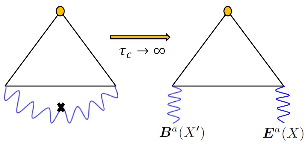
Figure 1: The triangle diagram with finite $\tau_{c}$ and with $\tau_{c}\rightarrow\infty$ in the constant-field limit. The blobs denote the axial vertices and the wiggly line with a cross at the center represents the correlator of color fields originating from the medium.

It is found $\partial_{\mu}J^{\mu}_{5}(X)\neq 0$ as opposed to the conservation of a vector charge current, $\partial_{\mu}J^{\mu}_{V}(X)=0$, implied by Eq. (64) since the diffusion term can be recast into a total momentum derivative including the attached $\delta(p^{2}-m^{2})$ due to $p^{\kappa}\mathscr{D}_{\kappa}[O]=0$. Now, Eq. (101) seems to be in connection to the chiral anomaly but it also receives the finite-mass correction. Recall that

$$\partial_{\mu}J^{\mu}_{5}(X)=-\frac{E\cdot B}{2\pi^{2}}+2m\langle\bar{\psi}i\gamma_{5}\psi\rangle$$ (102)

for massive fermions, where we consider the Abelian gauge fields for simplicity yet the similar feature holds for non-Abeleian cases. Here the pseudo-scalar condensate results in further modifications when $m\neq 0$. However, it is anticipated that $\partial_{\mu}J^{\mu}_{5}(X)=0$ when $m\rightarrow\infty$. For example, in the vacuum with constant electromagnetic fields, it is found Copinger et al. (2018),

$$\langle\bar{\psi}i\gamma_{5}\psi\rangle=\frac{E\cdot B}{4\pi^{2}m}\Big{(}1-e^{-\pi m^{2}/|E|}\Big{)}$$ (103)

and hence

$$\partial_{\mu}J^{\mu}_{5}(X)=-\frac{E\cdot B}{2\pi^{2}}e^{-\pi m^{2}/|E|}.$$ (104)

As shown in Eq. (101), $\partial_{\mu}J^{\mu}_{5}(X)=0$ when $m\rightarrow\infty$. In fact, from Eq. (101), we can extract the pseudo-scalar condensate,

$$\langle\bar{\psi}i\gamma_{5}\psi\rangle=-\frac{\hbar\langle B^{a}\cdot E^{a}\rangle}{8m\pi^{2}}\int^{\infty}_{0}d|\bm{p}|\left(1-\frac{|\bm{p}|}{\epsilon_{\bm{p}}}\right)\frac{d}{d|\bm{p}|}\big{[}f_{\rm eq}(\epsilon_{\bm{p}})-f_{\rm eq}(-\epsilon_{\bm{p}})\big{]},$$ (105)

such that Eq. (101) is decomposed as

$$\partial_{\mu}J_{5}^{\mu}(X)=-\hbar\frac{\langle B^{a}\cdot E^{a}\rangle}{4\pi^{2}}+2m\langle\bar{\psi}i\gamma_{5}\psi\rangle,$$ (106)

where the first term on the right-hand side above is given by

$$\frac{\hbar}{2}\langle B^{a}\cdot E^{a}\rangle\int^{\infty}_{0}\frac{d|\bm{p}|}{4\pi^{2}}\frac{d}{d|\bm{p}|}\big{[}f_{\rm eq}(|\bm{p}|)-f_{\rm eq}(-|\bm{p}|)\big{]}$$

$$=\frac{\hbar}{4\pi^{2}}\langle B^{a}\cdot E^{a}\rangle\big{[}f_{\rm eq}(|\bm{p}|)-f_{\rm eq}(-|\bm{p}|)\big{]}\Big{|}^{|\bm{p}|=\infty}_{|\bm{p}|=0}$$

$$=-\frac{\hbar}{4\pi^{2}}\langle B^{a}\cdot E^{a}\rangle.$$ (107)

Naively, when taking $m\rightarrow 0$, it seems $m\langle\bar{\psi}i\gamma_{5}\psi\rangle\rightarrow 0$ and the non-Abelian axial anomaly is reproduced in the massless limit. Nevertheless, since we work in the rest frame $n^{\mu}=n^{\mu}_{r}(p)$, the result is in principle subject to a finite-mass regime $m^{2}\gg|E^{a}|,\,|B^{a}|$. We may have to examine the massless limit more rigorously as will be demonstrated in the follow-up section.

VI Massless fermions

In order to investigate the influence of chromo-electromagnetic fields upon light quarks in QGP. We further analyze the similar effects on spin polarization of massless quarks via the CKT with non-Abelian gauge fields to complement the previous study for massive quarks.

VI.1 Derivation of the effective AKE

For massless fermions, it is more convenient to work in the chiral bases and the master equations reduce to

$$\hat{\nabla}\cdot\mathcal{W}_{s}=0,$$ (108)

$$\hat{\Pi}\cdot\mathcal{W}_{s}=0,$$ (109)

$$\hat{\Pi}_{\nu}\mathcal{W}_{s\mu}-\hat{\Pi}_{\mu}\mathcal{W}_{s\nu}=\frac{s\hbar}{2}\epsilon_{\mu\nu\rho\sigma}\hat{\nabla}^{\rho}\mathcal{W}_{s}^{\sigma},$$ (110)

where $\mathcal{W}_{s\mu}(p,X)$ denote the chiral components of Wigner operators (lesser propagators) for massless fermions with $s=1$ and $s=-1$ for right and left handed fermions (not to confuse with the superscript $\rm s$ for color singlet). Unlike the case for Dirac fermions, $\mathcal{W}_{s}$ are $2\times 2$ matrices in spinor space, which can be decomposed as $\mathcal{W}_{+}=\bar{\sigma}^{\mu}\mathcal{W}_{+\mu}$ and $\mathcal{W}_{-}=\sigma^{\mu}\mathcal{W}_{-\mu}$, where $\sigma^{\mu}=(1,{\bm{\sigma}})$ and $\bar{\sigma}^{\mu}=(1,-{\bm{\sigma}})$ with $\sigma^{i}$ being Pauli matrices. Based on the $\hbar$ expansion, the master equations explicit read

$$D\cdot\mathcal{W}_{s}+\frac{1}{2}\{F_{\nu\mu},\partial_{p}^{\nu}\mathcal{W}_{s}^{\mu}\}_{\rm c}-\frac{i\hbar}{24}[(\partial_{p}\cdot DF_{\nu\mu}),\partial_{p}^{\nu}\mathcal{W}_{s}^{\mu}]_{\rm c}=0,$$ (111)

$$p_{\mu}\mathcal{W}_{s}^{\mu}+\frac{i\hbar}{8}[F_{\nu\mu},\partial_{p}^{\nu}\mathcal{W}_{s}^{\mu}]_{\rm c}=0,$$ (112)

$$p_{[\nu}\mathcal{W}_{s\mu]}+\frac{i\hbar}{8}[F_{\rho[\nu},\partial_{p}^{\rho}\mathcal{W}_{s\mu]}]_{\rm c}=\frac{s\hbar}{2}\epsilon_{\mu\nu\rho\sigma}\Big{(}D^{\rho}\mathcal{W}_{s}^{\sigma}+\frac{1}{2}\{F_{\nu\mu},\partial_{p}^{\nu}\mathcal{W}_{s}^{\sigma}\}_{\rm c}\Big{)},$$ (113)

up to $\mathcal{O}(\hbar)$. By contracting Eq. (113) with $n^{\mu}$, one can derive the Wigner operator satisfying the constrain in Eq. (112). It is found

$$\mathcal{W}_{s}^{\mu} = 2\pi\bigg{[}\delta(p^{2})\Big{(}p^{\mu}\hat{f}_{s}+s\hbar S^{\mu\nu}_{(n)}\tilde{\Delta}_{\nu}\hat{f}_{s}\Big{)}+\frac{s\hbar}{2}p_{\nu}\delta^{\prime}(p^{2})\{\tilde{F}^{\mu\nu},\hat{f}_{s}\}_{\rm c}+\frac{i\hbar}{8}\bigg{(}p^{\mu}\delta^{\prime}(p^{2})p^{\rho}[F_{\nu\rho},\partial_{p}^{\nu}\hat{f}_{s}]_{\rm c}$$ (114)

$$+[F^{\rho\mu},\partial_{p\rho}\delta(p^{2})\hat{f}_{s}]_{\rm c}-\frac{2\delta(p^{2})}{p\cdot n}[F^{\mu\nu}n_{\nu},\hat{f}_{s}]_{\rm c}\bigg{)}\bigg{]}$$

up to $\mathcal{O}(\hbar)$, where $S^{\mu\nu}_{(n)}=S^{\mu\nu}_{m(n)}|_{m=0}$ represents the spin tensor for massless fermions. When making a conversion to the vector and axial-vector basis by $(\mathcal{V}/\mathcal{A})^{\mu}=(\mathcal{W}^{\mu}_{+}\pm\mathcal{W}^{\mu}_{-})/2$, one finds

$$\mathcal{A}^{\mu} = 2\pi\bigg{[}\delta(p^{2})\Big{(}p^{\mu}\hat{f}_{A}+\hbar S^{\mu\nu}_{(n)}\tilde{\Delta}_{\nu}\hat{f}_{V}\Big{)}+\frac{\hbar}{2}p_{\nu}\delta^{\prime}(p^{2})\{\tilde{F}^{\mu\nu},\hat{f}_{V}\}_{\rm c}+\frac{i\hbar}{8}\bigg{(}p^{\mu}\delta^{\prime}(p^{2})p^{\rho}[F_{\nu\rho},\partial_{p}^{\nu}\hat{f}_{A}]_{\rm c}$$ (115)

$$+[F^{\rho\mu},\partial_{p\rho}\delta(p^{2})\hat{f}_{A}]_{\rm c}-\frac{2\delta(p^{2})}{p\cdot n}[F^{\mu\nu}n_{\nu},\hat{f}_{A}]_{\rm c}\bigg{)}\bigg{]},$$

where $\hat{f}_{V/A}=(\hat{f}_{+}\pm\hat{f}_{-})/2$. Notably, the $\hbar$ terms related to commutators in color space are all linear to $\hat{f}_{A}$. As a result, implementing the power counting $\hat{f}_{V}\sim\mathcal{O}(\hbar^{0})$ and $\hat{f}_{A}\sim\mathcal{O}(\hbar)$, such terms involving commutators are suppressed. Similarly, the contribution from the last term on the left hand side of Eq. (111) in AKE is now of $\mathcal{O}(\hbar^{2})$ and hence omitted. That is, the effective AKE is given by

$$\tilde{\Delta}\cdot\mathcal{A}=D\cdot\mathcal{A}+\frac{1}{2}\{F_{\nu\mu},\partial_{p}^{\nu}\mathcal{A}^{\mu}\}_{\rm c}=0,$$ (116)

with

$$\mathcal{A}^{\mu}=2\pi\bigg{[}\delta(p^{2})\Big{(}p^{\mu}\hat{f}_{A}+\hbar S^{\mu\nu}_{(n)}\tilde{\Delta}_{\nu}\hat{f}_{V}\Big{)}+\frac{\hbar}{2}p_{\nu}\delta^{\prime}(p^{2})\{\tilde{F}^{\mu\nu},\hat{f}_{V}\}_{\rm c}\bigg{]},$$ (117)

which corresponds to the massless limit of Eq. (29) with $\hat{a}^{\mu}=p^{\mu}\hat{f}_{A}$ due to the spin locking by helicity. Note that the $\mathcal{A}^{\mu}$ in Eq. (117) is consistent with the result in Ref. Luo and Gao (2021) . As opposed to the massive case, one is now unable to choose the particle rest frame for $n^{\mu}$. Consequently, the magnetization-current term pertinent to $S^{\mu\nu}_{(n)}$ or the so-called side-jump term Chen et al. (2014b); Hidaka et al. (2017) in the massless limit will be always involved. For $\mathcal{V}^{\mu}$, we simply retain the leading-order term of $\mathcal{O}(\hbar^{0})$ and thus have $\mathcal{V}^{\mu}=2\pi\delta(p^{2})p^{\mu}\hat{f}_{V}$. Also, the SKE is same as Eq. (28) with the massless on-shell condition.

Inserting Eq. (117) into Eq. (116), the AKE turns out to be

$$0 = \delta(p^{2})\Big{(}p\cdot\tilde{\Delta}\hat{f}_{A}+\hbar\big{(}\tilde{\Delta}_{\mu}S^{\mu\nu}_{(n)}\big{)}\tilde{\Delta}_{\nu}\hat{f}_{V}+\hbar S^{\mu\nu}_{(n)}\tilde{\Delta}_{\mu}\tilde{\Delta}_{\nu}\hat{f}_{V}\Big{)}+\hbar\delta^{\prime}(p^{2})S^{\mu\nu}_{(n)}p^{\rho}\{F_{\rho\mu},\tilde{\Delta}_{\nu}\hat{f}_{V}\}$$ (118)

$$+\frac{\hbar}{2}\delta^{\prime}(p^{2})p_{\nu}\tilde{\Delta}_{\mu}\{\tilde{F}^{\mu\nu},\hat{f}_{V}\}_{\rm c}+\frac{\hbar}{4}\big{(}\partial_{p}^{\rho}p_{\nu}\delta^{\prime}(p^{2})\big{)}\{F_{\rho\mu},\{\tilde{F}^{\mu\nu},\hat{f}_{V}\}\}_{\rm c}\Big{)}.$$

We may now compute each term above. For the $\hbar$ corrections pertinent to $\delta(p^{2})$, it is found

$$\big{(}\tilde{\Delta}_{\mu}S^{\mu\nu}_{(n)}\big{)}\tilde{\Delta}_{\nu}\hat{f}_{V}=(\partial_{\mu}S^{\mu\nu}_{(n)})\tilde{\Delta}_{\nu}\hat{f}_{V}+\frac{1}{2p\cdot n}\Big{(}\{\tilde{F}^{\nu\beta}n_{\beta},\tilde{\Delta}_{\nu}\hat{f}_{V}\}_{\rm c}-S^{\mu\nu}_{(n)}\{n^{\rho}F_{\rho\mu},\tilde{\Delta}_{\nu}\hat{f}_{V}\}_{\rm c}\Big{)},$$ (119)

and

$$S^{\mu\nu}_{(n)}\tilde{\Delta}_{\mu}\tilde{\Delta}_{\nu}\hat{f}_{V}=\frac{S^{\mu\nu}_{(n)}}{2}\Big{(}i[F_{\mu\nu},\hat{f}_{V}]_{\rm c}+\frac{1}{2}\{(D_{[\mu}F_{\beta\nu]}),\partial^{\beta}_{p}\hat{f}_{V}\}_{\rm c}+\frac{1}{4}[F_{\alpha[\mu}F_{\beta\nu]},\partial^{\alpha}_{p}\partial^{\beta}_{p}\hat{f}_{V}]_{\rm c}\Big{)}.$$ (120)

On the other hand, for $\delta^{\prime}(p^{2})$ related terms, we acquire

$$\delta^{\prime}(p^{2})S^{\mu\nu}_{(n)}p^{\rho}\{F_{\rho\mu},\tilde{\Delta}_{\nu}\hat{f}_{V}\} = -\frac{\delta^{\prime}(p^{2})p_{\nu}}{2}\{\tilde{F}^{\mu\nu},\tilde{\Delta}_{\mu}\hat{f}_{V}\}_{\rm c}+\frac{\delta^{\prime}(p^{2})p_{\mu}n_{\nu}}{2p\cdot n}\{\tilde{F}^{\mu\nu},p\cdot\tilde{\Delta}\hat{f}_{V}\}_{\rm c}$$ (121)

$$-\frac{\delta(p^{2})}{2p\cdot n}\{\tilde{F}^{\nu\beta}n_{\beta},\tilde{\Delta}_{\nu}\hat{f}_{V}\}_{\rm c}$$

by using the Schouten identity and $p^{2}\delta^{\prime}(p^{2})=-\delta(p^{2})$. Also, one finds

$$\frac{\delta^{\prime}(p^{2})}{2}p_{\nu}\tilde{\Delta}_{\mu}\{\tilde{F}^{\mu\nu},\hat{f}_{V}\}_{\rm c}=\frac{\delta^{\prime}(p^{2})}{2}p_{\nu}\Big{(}\{\tilde{F}^{\mu\nu},\tilde{\Delta}_{\mu}\hat{f}_{V}\}_{\rm c}+\frac{1}{2}[[F_{\mu\rho},\tilde{F}^{\mu\nu}],\partial^{\rho}_{p}\hat{f}_{V}]_{\rm c}\Big{)}$$ (122)

by using

$$[A,\{B,C\}]=\{B,[A,C]\}+\{[A,B],C\},\quad\{A,\{B,C\}\}=\{B,\{A,C\}\}+[[A,B],C].$$ (123)

Finally, the last term is given by

$$\frac{1}{4}\big{(}\partial_{p}^{\rho}p_{\nu}\delta^{\prime}(p^{2})\big{)}\{F_{\rho\mu},\{\tilde{F}^{\mu\nu},\hat{f}_{V}\}\}_{\rm c}$$

$$=\frac{1}{4}\big{(}\delta^{\prime}(p^{2})\{F_{\nu\mu},\{\tilde{F}^{\mu\nu},\hat{f}_{V}\}\}_{\rm c}+2p_{\nu}p^{\rho}\delta^{\prime\prime}(p^{2})\{F_{\rho\mu},\{\tilde{F}^{\mu\nu},\hat{f}_{V}\}\}_{\rm c}\big{)}$$

$$=\frac{1}{2}\delta^{\prime\prime}(p^{2})p_{\nu}p^{\rho}[[\tilde{F}^{\mu\nu},F_{\rho\mu}],\hat{f}_{V}]_{\rm c},$$ (124)

where we have used

$$2p_{\nu}p^{\rho}\{F_{\rho\mu},\{\tilde{F}^{\mu\nu},\hat{f}_{V}\}\}_{\rm c}=-\frac{p^{2}}{2}\{F_{\mu\nu}\{\tilde{F}^{\mu\nu},\hat{f}_{V}\}\}_{\rm c}+2p_{\nu}p^{\rho}[[\tilde{F}^{\mu\nu},F_{\rho\mu}],\hat{f}_{V}]_{\rm c}$$ (125)

obtained from the Schouten identity and $p^{2}\delta^{\prime\prime}(p^{2})=-2\delta^{\prime}(p^{2})$. Combining all terms together, We eventually derive a free-streaming effective AKE for massless quarks coupled with background color fields

$$0 = \delta(p^{2})\bigg{[}p\cdot\tilde{\Delta}\hat{f}_{A}+\hbar(\partial_{\mu}S^{\mu\nu}_{(n)})\tilde{\Delta}_{\nu}\hat{f}_{V}+\frac{\hbar}{2p\cdot n}S^{\mu\nu}_{(n)}\{n^{\rho}F_{\mu\rho},\tilde{\Delta}_{\nu}\hat{f}_{V}\}_{\rm c}+\frac{\hbar S^{\mu\nu}_{(n)}}{2}\Big{(}i[F_{\mu\nu},\hat{f}_{V}]_{\rm c}$$ (126)

$$+\frac{1}{2}\{(D_{[\mu}F_{\beta\nu]}),\partial^{\beta}_{p}\hat{f}_{V}\}_{\rm c}+\frac{1}{4}[F_{\alpha[\mu}F_{\beta\nu]},\partial^{\alpha}_{p}\partial^{\beta}_{p}\hat{f}_{V}]_{\rm c}\Big{)}\bigg{]}+\frac{\hbar\delta^{\prime}(p^{2})p_{\mu}n_{\nu}}{2p\cdot n}\{\tilde{F}^{\mu\nu},p\cdot\tilde{\Delta}\hat{f}_{V}\}_{\rm c}$$

$$+\frac{\hbar\delta^{\prime}(p^{2})}{4}p_{\nu}[[F_{\mu\rho},\tilde{F}^{\mu\nu}],\partial^{\rho}_{p}\hat{f}_{V}]_{\rm c}+\frac{\hbar\delta^{\prime\prime}(p^{2})}{2}p_{\nu}p^{\rho}[[F_{\mu\rho},\tilde{F}^{\mu\nu}],\hat{f}_{V}]_{\rm c}.$$

VI.2 Spin diffusion and source terms

Implementing the color decomposition $\hat{f}_{V/A}=\hat{f}_{V/A}^{\rm s}I+\hat{f}_{V/A}^{a}t^{a}$ and taking $p\cdot\tilde{\Delta}\hat{f}_{V}=0$ from the off-shell SKE, the color-singlet and color-octet components of the AKE are given by

$$0 = \delta(p^{2})\bigg{[}p^{\mu}\mathcal{K}_{\rm s\mu}[\hat{f}_{A}]+\hbar(\partial_{\mu}S^{\mu\nu}_{(n)})\mathcal{K}_{\rm s\nu}[\hat{f}_{V}]+\frac{\hbar S^{\mu\nu}_{(n)}}{2p\cdot n}\bar{C}_{2}n^{\rho}F^{a}_{\mu\rho}\big{(}2\partial_{\nu}f_{V}^{a}+d^{abc}F^{b}_{\lambda\nu}\partial_{p}^{\lambda}\hat{f}_{V}^{c}\big{)}$$ (127)

$$+\hbar S^{\mu\nu}_{(n)}\Big{(}\bar{C}_{2}\big{(}(\partial_{\mu}F^{a}_{\beta\nu})-f^{abc}A^{b}_{\mu}F^{c}_{\beta\nu}\big{)}\partial_{p}^{\beta}\hat{f}_{V}^{a}\bigg{]},$$

and

$$0 = \delta(p^{2})\bigg{[}p^{\mu}\mathcal{K}^{a}_{\rm o\mu}[\hat{f}_{A}]+\hbar(\partial_{\mu}S^{\mu\nu}_{(n)})\mathcal{K}^{a}_{\rm o\mu}[\hat{f}_{V}]+\frac{\hbar}{2p\cdot n}S^{\mu\nu}_{(n)}n^{\rho}\big{(}2F^{a}_{\mu\rho}\mathcal{K}_{\rm s\nu}[\hat{f}_{V}]+d^{abc}F^{b}_{\mu\rho}\mathcal{K}^{c}_{\rm o\nu}[\hat{f}_{V}]\big{)}$$ (128)

$$+\hbar S^{\mu\nu}_{(n)}\big{(}(\partial_{\mu}F^{a}_{\beta\nu})-f^{abc}A^{b}_{\mu}F^{c}_{\beta\nu}\big{)}\partial^{\beta}_{p}\hat{f}^{\rm s}_{V}$$

$$-\frac{\hbar S^{\mu\nu}_{(n)}}{2}\Big{(}f^{abc}F^{b}_{\mu\nu}-d^{abc}\big{(}(\partial_{\mu}F^{b}_{\beta\nu})-f^{bef}A_{\nu}^{e}F^{f}_{\beta\nu}\big{)}\partial^{\beta}_{p}+\frac{f^{abc}f^{bef}}{4}F^{e}_{\alpha\mu}F^{f}_{\beta\nu}\partial^{\alpha}_{p}\partial^{\beta}_{p}\Big{)}\hat{f}^{c}_{V}\bigg{]}$$

$$-\frac{\hbar}{4}p_{\nu}f^{abc}f^{bef}F^{e}_{\mu\rho}\tilde{F}^{f\mu\nu}\Big{(}\delta^{\prime}(p^{2}-m^{2})\partial^{\rho}_{p}+2p^{\rho}\delta^{\prime\prime}(p^{2}-m^{2})\Big{)}\hat{f}_{V}^{c},$$

where

$$\mathcal{K}_{\rm s\mu}[O] \equiv \partial_{\mu}O^{s}+\bar{C}_{2}F^{a}_{\nu\mu}\partial_{p}^{\nu}O^{a},$$

$$\mathcal{K}^{a}_{\rm o\mu}[O] \equiv \partial_{\mu}O^{a}-f^{bca}A^{b}_{\mu}O^{c}+F^{a}_{\nu\mu}\partial^{\nu}_{p}O^{\rm s}+\frac{d^{bca}}{2}F^{b}_{\nu\mu}\partial_{p}^{\nu}O^{c}.$$ (129)

Given $\mathcal{O}^{a}\sim\mathcal{O}(g)$, Eq. (128) leads to

$$0\approx p^{\mu}\big{(}\partial_{\mu}\hat{f}_{A}^{a}-f^{bca}A^{b}_{\mu}\hat{f}^{c}_{A}+F^{a}_{\nu\mu}\partial^{\nu}_{p}\hat{f}_{V}^{\rm s}\big{)}+\hbar(\partial_{\mu}S^{\mu\nu}_{(n)})\partial_{\nu}\hat{f}^{a}_{V}+\hbar S^{\mu\nu}_{(n)}\Big{(}\frac{n^{\rho}F^{a}_{\mu\rho}}{p\cdot n}\partial_{\nu}+(\partial_{\mu}F^{a}_{\beta\nu})\partial_{p}^{\beta}\Big{)}\hat{f}^{s}_{V}$$ (130)

and thus

$$\hat{f}_{A}^{a}(p,X) = -\int^{ab,p}_{k,X^{\prime}}\Big{[}p^{\mu}F^{b}_{\nu\mu}(X^{\prime})\partial^{\nu}_{p}+\hbar S^{\mu\nu}_{(n)}\Big{(}\frac{n^{\rho}F^{b}_{\mu\rho}(X^{\prime})}{p\cdot n}\partial_{X^{\prime}\nu}+\big{(}\partial_{X^{\prime}\mu}F^{a}_{\beta\nu}(X^{\prime})\big{)}\partial_{p}^{\beta}\Big{)}\Big{]}\hat{f}^{s}_{V}(p,X^{\prime})$$ (131)

$$+\int^{ab,p}_{k,X^{\prime}}\hbar(\partial_{X^{\prime}\mu}S^{\mu\nu}_{(n)})\partial_{X^{\prime}\nu}\int^{bc,p}_{k^{\prime},X^{\prime\prime}}\Big{[}p^{\alpha}F^{c}_{\beta\alpha}(X^{\prime\prime})\partial^{\beta}_{X^{\prime\prime}p}\hat{f}^{\rm s}_{V}(p,X^{\prime\prime})\Big{]}$$

up to $\mathcal{O}(g)$, where we have employed Eq. (53) to rewrite $\hat{f}^{a}_{V}$ in terms of $\hat{f}^{s}_{V}$. For simplicity, we may work with a constant frame vector. Then Eq. (127) becomes

$$0 \approx \delta(p^{2})\bigg{[}p\cdot\partial\hat{f}^{\rm s}_{A}+\bar{C}_{2}p^{\mu}F^{a}_{\nu\mu}\partial^{\nu}_{p}\hat{f}^{a}_{A}+\frac{\hbar S^{\mu\nu}_{(n)}}{p\cdot n}\bar{C}_{2}n^{\rho}F^{a}_{\mu\rho}\partial_{\nu}\hat{f}_{V}^{a}+\hbar S^{\mu\nu}_{(n)}\bar{C}_{2}(\partial_{\mu}F^{a}_{\rho\nu})\partial_{p}^{\rho}\hat{f}_{V}^{a}\bigg{]}$$ (132)

up to $\mathcal{O}(g^{2})$. By replacing $\hat{f}^{a}_{V/A}$ with $\hat{f}^{\rm s}_{V/A}$ and taking the ensemble averages, we eventually derive

$$0=\delta(p^{2})\Big{(}p\cdot\partial f^{\rm s}_{A}(p,X)-\partial_{p}^{\kappa}\mathscr{D}_{\kappa}[f^{\rm s}_{A}]+\hbar\partial_{p}^{\sigma}\mathscr{B}_{\sigma}[f^{\rm s}_{V}]+\hbar S^{\mu\nu}_{(n)}\mathscr{C}_{\mu\nu}[f^{\rm s}_{V}]\Big{)},$$ (133)

where

$$\mathscr{B}_{\sigma}[O]=\bar{C}_{2}p^{\rho}S^{\mu\nu}_{(n)}\int^{p}_{k,X^{\prime}}\bigg{[}\big{(}\partial_{X^{\prime}\mu}\langle F^{a}_{\sigma\rho}(X)F^{a}_{\nu\lambda}(X^{\prime})\rangle\big{)}\partial_{p}^{\lambda}-\frac{n^{\lambda}}{p\cdot n}\langle F^{a}_{\sigma\rho}(X)F^{a}_{\nu\lambda}(X^{\prime})\rangle\partial_{X^{\prime}\mu}\bigg{]}O(p,X^{\prime})$$ (134)

and

$$\mathscr{C}_{\mu\nu}[O]=\bar{C}_{2}p^{\rho}\int^{p}_{k,X^{\prime}}\bigg{[}\frac{n^{\lambda}}{p\cdot n}\partial_{X^{\prime}\mu}\langle F^{a}_{\nu\lambda}(X)F^{a}_{\sigma\rho}(X^{\prime})\rangle+\partial_{X\mu}\langle F^{a}_{\nu\lambda}(X)F^{a}_{\sigma\rho}(X^{\prime})\rangle\partial^{\lambda}_{p}\bigg{]}\partial^{\sigma}_{p}O(p,X^{\prime}).$$ (135)

Here we have utilized

$$\bar{C}_{2}p^{\mu}\langle F^{a}_{\nu\mu}\partial^{\nu}_{p}\hat{f}^{a}_{A}\rangle = \hbar\bar{C}_{2}p^{\rho}\partial_{p}^{\sigma}\bigg{\{}S^{\mu\nu}_{(n)}\int^{p}_{k,X^{\prime}}\bigg{[}\big{(}\partial_{X^{\prime}\mu}\langle F^{a}_{\sigma\rho}(X)F^{a}_{\nu\lambda}(X^{\prime})\rangle\big{)}\partial^{\lambda}_{p}$$ (136)

$$-\frac{n^{\lambda}}{p\cdot n}\langle F^{a}_{\sigma\rho}(X)F^{a}_{\nu\lambda}(X^{\prime})\rangle\partial_{X^{\prime}\mu}\bigg{]}f^{\rm s}_{V}(p,X^{\prime})\bigg{\}},$$

$$\frac{\hbar S^{\mu\nu}_{(n)}}{p\cdot n}\bar{C}_{2}n^{\rho}\langle F^{a}_{\mu\rho}\partial_{\nu}\hat{f}_{V}^{a}\rangle=\frac{\hbar S^{\mu\nu}_{(n)}}{p\cdot n}\bar{C}_{2}n^{\lambda}\langle F^{a}_{\nu\lambda}(X)\partial_{X\mu}\int^{p}_{k,X^{\prime}}F^{a}_{\sigma\rho}(X^{\prime})\rangle\partial^{\sigma}_{p}f^{\rm s}_{V}(p,X^{\prime}),$$ (137)

$$\hbar S^{\mu\nu}_{(n)}\bar{C}_{2}\langle(\partial_{\mu}F^{a}_{\rho\nu})\partial_{p}^{\rho}\hat{f}_{V}^{a}\rangle=\hbar\bar{C}_{2}S^{\mu\nu}_{(n)}\partial^{\lambda}_{p}\int^{p}_{k,X^{\prime}}p^{\rho}\partial_{X\mu}\langle F^{a}_{\nu\lambda}(X)F^{a}_{\sigma\rho}(X^{\prime})\rangle\partial_{p}^{\sigma}f^{\rm s}_{V}(p,X^{\prime}),$$ (138)

and have assumed the relation

$$\partial_{X\mu}\int^{p}_{k,X^{\prime}}G(X^{\prime})=-i\int^{p}_{k,X^{\prime}}k_{\mu}G(X^{\prime})=\int^{p}_{k,X^{\prime}}\partial_{X^{\prime}\mu}G(X^{\prime})$$ (139)

given $e^{ik\cdot X^{\prime}}G(X^{\prime})\big{|}_{X^{\prime\mu}=\pm\infty}=0$ for an arbitrary function $G(X^{\prime})$ is applicable for Eq. (137).

Although the $\hbar$ correction, corresponding to the source term for dynamical spin polarization, in the AKE for massless quarks takes a slightly different form compared to that for massive fermions, they both stem from spacetime variations of color fields. On the other hand, the color-singlet axial-vector component of the Wigner function reads

$$\langle\mathcal{A}^{\rm s\mu}\rangle = 2\pi\bigg{\{}\delta(p^{2})\bigg{[}p^{\mu}f^{\rm s}_{A}+\hbar S^{\mu\nu}_{(n)}\big{(}\partial_{\nu}f_{V}^{\rm s}+\bar{C}_{2}\langle F^{a}_{\rho\nu}\partial_{p}^{\rho}\hat{f}_{V}^{a}\rangle\big{)}-\frac{\hbar\bar{C}_{2}}{2}\langle\tilde{F}^{a\mu\nu}\partial_{p\nu}\hat{f}^{a}_{V}\rangle\bigg{]}$$ (140)

$$+\frac{\hbar\bar{C}_{2}}{2}\partial_{p\nu}\big{(}\delta(p^{2})\langle\tilde{F}^{a\mu\nu}\hat{f}^{a}_{V}\rangle\big{)}\bigg{\}},$$

which yields the color singlet of the on-shell axial charge current density in phase space,

$$\mathcal{A}^{\rm s\mu}(\bm{p},X)\equiv\int\frac{dp_{0}}{2\pi}\langle\mathcal{A}^{\rm s\mu}\rangle=\frac{1}{2|\bm{p}|}\big{(}p^{\mu}f_{A}^{\rm s}+\hbar\bar{C}_{2}\tilde{\mathcal{A}}^{\mu}_{Q}\big{)}_{p_{0}=|\bm{p}|},$$ (141)

where $\tilde{\mathcal{A}}^{\mu}_{Q}=\tilde{\mathcal{A}}^{\mu}_{Q_{1}}+\tilde{\mathcal{A}}^{\mu}_{Q2}+\tilde{\mathcal{A}}^{\mu}_{Q3}$ with $\tilde{\mathcal{A}}^{\mu}_{Q1}=\mathcal{A}^{\mu}_{Q1}|_{m=0}$, $\tilde{\mathcal{A}}^{\mu}_{Q2}=\mathcal{A}^{\mu}_{Q2}|_{m=0}$, and

$$\tilde{\mathcal{A}}^{\mu}_{Q3}(\bm{p},X) = -\bigg{[}S^{\mu\nu}_{(n)}\partial_{p}^{\rho}\int^{p}_{k,X^{\prime}}p^{\beta}\langle F^{a}_{\rho\nu}(X)F_{\alpha\beta}(X^{\prime})\rangle\partial^{\alpha}_{p}f_{V}^{\rm s}(p,X^{\prime})\bigg{]}_{p_{0}=|\bm{p}|},$$ (142)

which also contain the source terms coming from $\hbar$ corrections for spin polarization.

VI.3 Spin polarization, axial charge currents, and axial Ward identity

We may now also investigate the spin polarization, axial charge current, and axial Ward identity of massless fermions for $f^{\rm s}_{V}$ near equilibrium with negligible gradient corrections in hydrodynamics. In such a case, it is more convenient to choose $n^{\mu}=u^{\mu}$ and work in the fluid rest frame . We re-emphasize that the Wigner function is however independent of the choice of a frame. Moreover, we may consider the color-field correlators only depending on $\delta X_{0}$ with the temporal direction now defined in the fluid rest frame. Notably, since $S^{\mu\nu}_{(n)}\partial_{\delta X\nu}\Phi(\delta X_{0})=0$ for $n^{\mu}=u^{\mu}\approx(1,\bm{0})$, it turns out that the source term in Eq. (133) vanishes in our particular setup. In such a case, $f_{A}^{s}$ should simply diffuse to zero in equilibrium given no vortical corrections. When $f^{\rm s}_{V}$ is in equilibrium and $f^{\rm s}_{A}=0$, Eq. (140) reduces to

$$\hat{\mathcal{A}}^{\rm s\mu}(\bm{p},X)=\hbar\bar{C}_{2}\big{(}\tilde{\mathcal{A}}^{\mu}_{Q1}(\bm{p},X)+\tilde{\mathcal{A}}^{\mu}_{Q2}(\bm{p},X)+\tilde{\mathcal{A}}^{\mu}_{Q3}(\bm{p},X)\big{)},$$ (143)

where $\tilde{\mathcal{A}}^{\mu}_{Q1}(\bm{p},X)+\tilde{\mathcal{A}}^{\mu}_{Q2}(\bm{p},X)$ is nothing but Eq. (91) with $m=0$, and

$$\tilde{\mathcal{A}}^{\mu}_{Q3}(\bm{p},X)=\frac{\pi^{1/2}\tau_{c}}{2p_{0}}S^{\mu\nu}_{(n)}\langle E^{a}_{\nu}E^{a}_{\beta}\rangle\hat{p}^{\beta}\big{(}1-p_{0}\partial_{p0}\big{)}\partial_{p0}f_{\rm eq}(p_{0})\Big{|}_{p_{0}=|\bm{p}|}$$ (144)

by similarly assuming $\Phi(\delta X_{0})=e^{-\delta X_{0}^{2}/\tau_{c}^{2}}$ and working in the fluid-rest frame. When dropping the subleading correlation function of two color electric fields, the non-dynamical source term for spin polarization of massless quarks matches the one of massive quarks by simply taking $m=0$.

One can analogously evaluate the axial charge current for finite $\tau_{c}$, which reads

$$J^{\mu}_{5}(X) = -2\hbar\int\frac{d^{4}p}{(2\pi)^{3}}\frac{\delta(p^{2})}{2}\int^{p}_{k,X^{\prime}}\langle B^{a\rho}(X)E^{a}_{\rho}(X^{\prime})\rangle\beta u^{\mu}f_{\rm eq}(p\cdot u)(1-f_{\rm eq}(p\cdot u))$$ (145)

$$= 2\hbar\int\frac{d^{4}p}{(2\pi)^{3}}\frac{\delta(p^{2})}{4p\cdot u}\sqrt{\pi}\tau_{c}\langle E^{a}\cdot B^{a}\rangle u^{\mu}\partial_{p\cdot u}f_{\rm eq}(p\cdot u)$$

and agrees with the result for massive fermions by taking $m=0$ and hence $\partial\cdot J_{5}=0$. In the limit for $\tau_{c}\rightarrow\infty$, following the previous calculations for massive fermions and taking $\langle B^{a\rho}(X)E^{a}_{\rho}(X^{\prime})\rangle=\langle B^{a}\cdot E^{a}\rangle$, it turns out that

$$\partial_{\mu}J^{\mu}_{5}(X)=-\frac{\hbar}{4\pi^{2}}\langle B^{a}\cdot E^{a}\rangle,$$ (146)

which corresponds to the non-Abelian axial anomaly as expected.

VII Summary and discussions

Here we briefly summarize the primary findings. We have derived the AKE containing a classical spin diffusion term and a source term from quantum corrections that could possibly trigger spin polarization for massive quarks (with mass greater than the gradient scales) as shown in Eq. (60). A similar equation for massless quarks is also derived in Eq. (133). On the other hand, there also exist explicit quantum corrections in Wigner functions, which severe as the additional source terms to generate spin polarization shown in Eqs. (67) and (141) for massive and massless quarks, respectively. Given postulated color-field correlators based on spacetime translational invariance and spatial homogeneity, the parity-odd correlators of color fields, depending on their time difference can dominantly generate nonzero spin polarization as shown in Eq. (92) for massive fermions near thermal equilibrium. Such a contribution further results in a nonzero axial charge current or more precisely the axial charge density in the fluid rest frame. This constant axial charge current also gives the vanishing axial Ward identity with finite correlation time of the color-field correlators. However, in the constant-field limit with infinite correlation time, the nonzero axial Ward identity associated with the pseudo-scalar condensate at finite temperature is acquired as shown in Eq. (106). For massless fermions, a particular frame choice leads to the vanishing dynamical source term in AKE, while there exists a similar non-dynamical source term for spin polarization in the Wigner function. Note that the choice of a frame is simply for the technical reason, which does not affect the physical observables in the end. The axial Ward identity reduces to the expected axial anomaly as manifested by Eq. (146) in the constant-field limit as anticipated. In order to make a smooth connection between the results of the massive and massless quarks, it is necessary to further work out the AKT of massive quarks in a proper frame for arbitrary mass such as $n^{\mu}=u^{\mu}$ for $f^{s}_{V}$ near equilibrium.

In phenomenology, as proposed in Ref. Müller and Yang (2022), such spin polarization of quarks engendered by color-field correlators could potentially affect the spin alignment of vector mesons observed in heavy ion collisions Acharya et al. (2020); Singha (2021) as an unsettled question in theory (see Refs .Sheng et al. (2020a, b); Xia et al. (2021); Gonçalves and Torrieri (2022) for other theoretical explanations). In order to make direct comparisons with experimental data, it is necessary to incorporate the color-field correlators from real-time simulations with prescribed initial conditions. According to the approximations adopted in Ref. Müller and Yang (2022) and this work, the parity-odd correlator between a chromo-magnetic field and a chromo-electric field is essential to generate spin polarization for massive quarks. However, due to the event-by-event fluctuations of the sign for such a correlator, the anomalous spin polarization by turbulent color fields may contribute to spin alignment of vector mesons, coming from the product of spin polarization for a quark and for an anti-quark, without affecting the spin polarization of Lambda hyperons. Further studies on simulations or more practical estimation of color-field correlators and the generalization of present QKT with source terms to arbitrary quark mass will be needed.

Appendix A Details of integration

In this appendix, we will consider the relevant integral of an arbitrary function $\tilde{G}(p,X,X^{\prime})=G(p,X,\delta X)$. For brevity, we will simply denote $G(p,X,\delta X)=G(X,\delta X)$, while the $p$ dependence has to be taken into account in the end. We now consider the integral

$$I_{k,X^{\prime}}\equiv\int d^{4}k\int\frac{d^{4}X^{\prime}}{(2\pi)^{4}}\frac{e^{ik\cdot(X^{\prime}-X)}}{p\cdot k}\tilde{G}(X,X^{\prime})=\int d^{4}k\int\frac{d^{4}\delta X}{(2\pi)^{4}}\frac{e^{-ik\cdot\delta X}}{p\cdot k}G(X,\delta X),$$ (147)

where $\delta X\equiv X-X^{\prime}$. Assigning $p_{\mu}=(p_{0},0,0,p_{z})$, it is found

$$I_{k,X^{\prime}} = \int\frac{d^{4}\delta X}{(2\pi)^{2}}\int dk_{0}dk_{z}\frac{e^{-ik_{0}\delta X_{0}+ik_{z}\delta X_{z}}}{p_{0}k_{0}-p_{z}k_{z}}\delta^{2}(\delta X_{\rm T})G(X,\delta X)$$ (148)

$$= \int\frac{d^{4}\delta X}{(2\pi)^{2}}\int dk_{z}d\tilde{k}_{0}\frac{e^{-i\tilde{k}_{0}\delta X_{0}-i\frac{p_{z}k_{z}}{p_{0}}\delta X_{0}+ik_{z}\delta X_{z}}}{p_{0}\tilde{k}_{0}}\delta^{2}(\delta X_{\rm T})G(X,\delta X)$$

$$= -i\pi\int\frac{d^{4}\delta X}{(2\pi)}\delta\left(\frac{p_{z}}{p_{0}}\delta X_{0}-\delta X_{z}\right)\frac{{\rm sgn}(\delta X_{0})}{p_{0}}\delta^{2}(\delta X_{\rm T})G(X,\delta X),$$

where $\delta X_{\rm T}$ are the transverse components of $\delta X_{\mu}$ with respect to $p_{\mu}$, $\tilde{k}_{0}=k_{0}-p_{z}k_{z}/p_{0}$, and we have utilized the Fourier transform

$$\int_{-\infty}^{\infty}dxe^{-ikx}/x=-i\pi{\rm sgn}(k).$$ (149)

Integrating over $\delta X_{\rm T}$ and $\delta X_{z}$, one finally obtains

$$I_{k,X^{\prime}}=-\frac{i}{2p_{0}}\int d\delta X_{0}\Big{[}{\rm sgn}(\delta X_{0})G(X,\delta X)\Big{]}_{\delta X_{T}=0,\delta X_{z}=p_{z}\delta X_{0}/p_{0}}.$$ (150)

It turns out that $I_{k,X^{\prime}}$ is non-vanishing only when $G(X,\delta X)$ is an odd function of $\delta X_{0}$ or of $\delta X_{z}$.

On the contrary, we shall consider the integral

$$I^{+}_{k,X^{\prime}}\equiv\lim_{\epsilon\rightarrow 0}\int d^{4}k\int\frac{d^{4}\delta X}{(2\pi)^{4}}\frac{e^{-ik\cdot\delta X}}{p\cdot k+i\epsilon}G(X,\delta X),$$ (151)

where $\epsilon>0$. By employing the decomposition,

$$\frac{1}{p\cdot k+i\epsilon}=\frac{p\cdot k}{(p\cdot k)^{2}+\epsilon^{2}}-\frac{i\epsilon}{(p\cdot k)^{2}+\epsilon^{2}},$$ (152)

we may also decompose $I^{+}_{k,X^{\prime}}$ into

$$I^{+}_{k,X^{\prime}}=I^{+(1)}_{k,X^{\prime}}+I^{+(2)}_{k,X^{\prime}},$$ (153)

where

$$I^{+(1)}_{k,X^{\prime}}=\lim_{\epsilon\rightarrow 0}\int d^{4}k\int\frac{d^{4}\delta X}{(2\pi)^{4}}\frac{p\cdot ke^{-ik\cdot\delta X}}{(p\cdot k)^{2}+\epsilon^{2}}G(X,\delta X)$$ (154)

and

$$I^{+(2)}_{k,X^{\prime}}=\lim_{\epsilon\rightarrow 0}\int d^{4}k\int\frac{d^{4}\delta X}{(2\pi)^{4}}\frac{-i\epsilon e^{-ik\cdot\delta X}}{(p\cdot k)^{2}+\epsilon^{2}}G(X,\delta X).$$ (155)

Using

$$\lim_{\epsilon\rightarrow 0}\frac{\epsilon}{x^{2}+\epsilon^{2}}=\pi\delta(x),$$ (156)

one immediately finds

$$I^{+(2)}_{k,X^{\prime}}=-i\pi\int d^{4}k\int\frac{d^{4}\delta X}{(2\pi)^{4}}\delta(p\cdot k)e^{-ik\cdot\delta X}G(X,\delta X).$$ (157)

To evaluate $I^{+(1)}_{k,X^{\prime}}$, we assign $p_{\mu}=(p_{0},0,0,p_{z})$ and hence

$$I^{+(1)}_{k,X^{\prime}}=\lim_{\epsilon\rightarrow 0}\int dk_{0}dk_{z}\int\frac{d\delta X_{0}d\delta X_{z}}{(2\pi)^{2}}\frac{(p_{0}k_{0}-p_{z}k_{z})e^{-ik_{0}\delta X_{0}+ik_{z}\delta X_{z}}}{(p_{0}k_{0}-p_{z}k_{z})^{2}+\epsilon^{2}}G(X,\delta X)|_{\delta X_{x,y}=0},$$ (158)

where we have integrated over $k_{x,y}$ and then $\delta X_{x,y}$. We then first take the limit of the integrand,

$$\lim_{\epsilon\rightarrow 0}\frac{(p_{0}k_{0}-p_{z}k_{z})e^{-ik_{0}\delta X_{0}+ik_{z}\delta X_{z}}}{(p_{0}k_{0}-p_{z}k_{z})^{2}+\epsilon^{2}}=\frac{e^{-ik_{0}\delta X_{0}+ik_{z}\delta X_{z}}}{(p_{0}k_{0}-p_{z}k_{z})}$$ (159)

and subsequently integrate over $k_{0}$ by using

$$\int_{-\infty}^{\infty}dke^{-ikx}/(k+a)=-i\pi{\rm sgn}(x)e^{ika}.$$ (160)

It is found

$$I^{+(1)}_{k,X^{\prime}} = -i\pi\int dk_{z}\int\frac{d\delta X_{0}d\delta X_{z}}{(2\pi)^{2}}\frac{{\rm sgn}(\delta X_{0})}{p_{0}}e^{ik_{z}(\delta X_{z}-\delta X_{0}p_{z}/p_{0})}G(X,\delta X)|_{\delta X_{x,y}=0}$$ (161)

$$= -i\pi\int\frac{d\delta X_{0}d\delta X_{z}}{(2\pi)}\frac{{\rm sgn}(\delta X_{0})}{p_{0}}\delta\big{(}\delta X_{z}-\delta X_{0}p_{z}/p_{0}\big{)}G(X,\delta X)|_{\delta X_{x,y}=0}$$

$$= -\frac{i}{2p_{0}}\int d\delta X_{0}\Big{[}{\rm sgn}(\delta X_{0})G(X,\delta X)\Big{]}_{\delta X_{x,y}=0,\delta X_{z}=p_{z}\delta X_{z}/p_{0}}.$$

which agrees with Eq. (150). Similarly, from Eq. (157), one can also obtain

$$I^{+(2)}_{k,X^{\prime}} = -\frac{i}{2p_{0}}\int d\delta X_{0}G(X,\delta X)|_{\delta X_{x,y}=0,\delta X_{z}=p_{z}\delta X_{0}/p_{0}},$$ (162)

and hence

$$I^{+}_{k,X^{\prime}} = -\frac{i}{2p_{0}}\int d\delta X_{0}\Big{(}1+{\rm sgn}(\delta X_{0})\Big{)}G(X,\delta X)|_{\delta X_{x,y}=0,\delta X_{z}=p_{z}\delta X_{0}/p_{0}},$$ (163)

Eventually, the principle value part of $1/(p\cdot k+i\epsilon)$ should still contribute to the integral $I^{+}_{k,X^{\prime}}$. Nevertheless, when $G(X,\delta X)$ is an even function of $\delta X_{0,z}$, only $I^{+(2)}_{k,X^{\prime}}$ yields a non-vanishing result. The conclusion is then consistent with the finding in Ref. Asakawa et al. (2007).

Recall that $G(X,\delta X)=G(p,X,\delta X)$. Given

$$I^{+}_{k,X^{\prime}}=-i\int^{p}_{k,X^{\prime}}G(X,\delta X)=-\frac{i}{2p_{0}}\int d\delta X_{0}\Big{(}1+{\rm sgn}(\delta X_{0})\Big{)}G(X,\delta X)|_{\delta X_{c}},$$ (164)

where $\delta X_{c}\equiv\{\delta X_{x,y}=0,\delta X_{z}=p_{z}\delta X_{0}/p_{0}\}$, it is found

$$\partial_{p\kappa}I^{+}_{k,X^{\prime}} = -\frac{\delta^{0}_{\kappa}}{p_{0}}I^{+}_{k,X^{\prime}}-\frac{i}{2p_{0}}\int d\delta X_{0}\Big{(}1+{\rm sgn}(\delta X_{0})\Big{)}\partial_{p\kappa}\big{(}G(X,\delta X)|_{\delta X_{c}}\big{)}.$$ (165)

Using the chain rule,

$$\partial_{p\kappa}\big{(}G(X,\delta X)|_{\delta X_{c}}\big{)}=\big{(}\partial_{p\kappa}G(X,\delta X)\big{)}_{\delta X_{c}}+\big{(}\partial_{\delta X_{z}}G(X,\delta X)\big{)}_{\delta X_{c}}\delta X_{0}\partial_{p\kappa}(p_{z}/p_{0}).$$ (166)

one finds another useful relation,

$$\partial_{p\kappa}\int^{p}_{k,X^{\prime}}G(X,\delta X) = -\frac{\delta^{0}_{\kappa}}{p_{0}}\int^{p}_{k,X^{\prime}}G(X,\delta X)+\int^{p}_{k,X^{\prime}}\partial_{p\kappa}G(X,\delta X)$$ (167)

$$+\int^{p}_{k,X^{\prime}}\delta X_{0}\frac{\partial G(X,\delta X)}{\partial\delta X^{\mu}_{\perp}}\partial_{p\kappa}\left(\frac{p_{\perp}^{\mu}}{p_{0}}\right)$$

for the off-shell integral. When imposing the on-shell condition first, an analogous relation reads

$$\partial_{p\kappa}\Big{(}\int^{p}_{k,X^{\prime}}G(X,\delta X)\Big{)}_{p_{0}=\epsilon_{\bm{p}}} = -\frac{p_{\perp\kappa}}{\epsilon_{\bm{p}}^{2}}\int^{\bm{p}}_{k,X^{\prime}}G(X,\delta X)_{p_{0}=\epsilon_{\bm{p}}}+\int^{\bm{p}}_{k,X^{\prime}}\partial_{p_{\perp}\kappa}G(X,\delta X)_{p_{0}=\epsilon_{\bm{p}}}$$ (168)

$$+\int^{\bm{p}}_{k,X^{\prime}}\delta X_{0}\left(\frac{\partial G(X,\delta X)}{\partial\delta X^{\mu}_{\perp}}\right)_{p_{0}=\epsilon_{\bm{p}}}\partial_{p_{\perp}\kappa}\left(\frac{p_{\perp}^{\mu}}{\epsilon_{\bm{p}}}\right),$$

where $\int^{\bm{p}}_{k,X^{\prime}}=\int^{p}_{k,X^{\prime}}\big{|}_{p_{0}=\epsilon_{\bm{p}}}$.

References

• Vilenkin (1980) A. Vilenkin, Phys. Rev. D22, 3080 (1980).
• Nielsen and Ninomiya (1983) H. B. Nielsen and M. Ninomiya, Phys. Lett. B 130, 389 (1983).
• Alekseev et al. (1998) A. Y. Alekseev, V. V. Cheianov, and J. Frohlich, Phys. Rev. Lett. 81, 3503 (1998), eprint cond-mat/9803346.
• Kharzeev (2006) D. Kharzeev, Phys.Lett. B633, 260 (2006), eprint hep-ph/0406125.
• Kharzeev et al. (2008) D. E. Kharzeev, L. D. McLerran, and H. J. Warringa, Nucl. Phys. A803, 227 (2008), eprint 0711.0950.
• Fukushima et al. (2008) K. Fukushima, D. E. Kharzeev, and H. J. Warringa, Phys. Rev. D78, 074033 (2008), eprint 0808.3382.
• Vilenkin (1979) A. Vilenkin, Phys. Rev. D20, 1807 (1979).
• Erdmenger et al. (2009) J. Erdmenger, M. Haack, M. Kaminski, and A. Yarom, JHEP 01, 055 (2009), eprint 0809.2488.
• Banerjee et al. (2011) N. Banerjee et al., JHEP 01, 094 (2011), eprint 0809.2596.
• Son and Surowka (2009) D. T. Son and P. Surowka, Phys. Rev. Lett. 103, 191601 (2009), eprint 0906.5044.
• Landsteiner et al. (2011) K. Landsteiner, E. Megias, and F. Pena-Benitez, Phys. Rev. Lett. 107, 021601 (2011), eprint 1103.5006.
• Adler (1969) S. L. Adler, Phys. Rev. 177, 2426 (1969).
• Bell and Jackiw (1969) J. S. Bell and R. Jackiw, Nuovo Cim. A 60, 47 (1969).
• Son and Yamamoto (2012) D. T. Son and N. Yamamoto, Phys. Rev. Lett. 109, 181602 (2012), eprint 1203.2697.
• Stephanov and Yin (2012) M. Stephanov and Y. Yin, Phys. Rev. Lett. 109, 162001 (2012), eprint 1207.0747.
• Chen et al. (2014a) J.-W. Chen, J.-y. Pang, S. Pu, and Q. Wang, Phys. Rev. D89, 094003 (2014a), eprint 1312.2032.
• Chen et al. (2014b) J.-Y. Chen, D. T. Son, M. A. Stephanov, H.-U. Yee, and Y. Yin, Phys. Rev. Lett. 113, 182302 (2014b), eprint 1404.5963.
• Chen et al. (2015) J.-Y. Chen, D. T. Son, and M. A. Stephanov, Phys. Rev. Lett. 115, 021601 (2015), eprint 1502.06966.
• Gao et al. (2012) J.-H. Gao, Z.-T. Liang, S. Pu, Q. Wang, and X.-N. Wang, Phys. Rev. Lett. 109, 232301 (2012), eprint 1203.0725.
• Chen et al. (2013) J.-W. Chen, S. Pu, Q. Wang, and X.-N. Wang, Phys. Rev. Lett. 110, 262301 (2013), eprint 1210.8312.
• Son and Yamamoto (2013) D. T. Son and N. Yamamoto, Phys. Rev. D87, 085016 (2013), eprint 1210.8158.
• Hidaka et al. (2017) Y. Hidaka, S. Pu, and D.-L. Yang, Phys. Rev. D95, 091901 (2017), eprint 1612.04630.
• Hidaka et al. (2018) Y. Hidaka, S. Pu, and D.-L. Yang, Phys. Rev. D97, 016004 (2018), eprint 1710.00278.
• Manuel and Torres-Rincon (2014a) C. Manuel and J. M. Torres-Rincon, Phys. Rev. D89, 096002 (2014a), eprint 1312.1158.
• Manuel and Torres-Rincon (2014b) C. Manuel and J. M. Torres-Rincon, Phys. Rev. D90, 076007 (2014b), eprint 1404.6409.
• Hidaka and Yang (2018) Y. Hidaka and D.-L. Yang, Phys. Rev. D98, 016012 (2018), eprint 1801.08253.
• Mueller and Venugopalan (2017) N. Mueller and R. Venugopalan, Phys. Rev. D96, 016023 (2017), eprint 1702.01233.
• Mueller and Venugopalan (2018) N. Mueller and R. Venugopalan, Phys. Rev. D97, 051901 (2018), eprint 1701.03331.
• Huang et al. (2018) A. Huang, S. Shi, Y. Jiang, J. Liao, and P. Zhuang, Phys. Rev. D98, 036010 (2018), eprint 1801.03640.
• Yang (2018) D.-L. Yang, Phys. Rev. D98, 076019 (2018), eprint 1807.02395.
• Liu et al. (2019) Y.-C. Liu, L.-L. Gao, K. Mameda, and X.-G. Huang, Phys. Rev. D99, 085014 (2019), eprint 1812.10127.
• Lin and Shukla (2019) S. Lin and A. Shukla, JHEP 06, 060 (2019), eprint 1901.01528.
• Lin and Yang (2020) S. Lin and L. Yang, Phys. Rev. D 101, 034006 (2020), eprint 1909.11514.
• Shi et al. (2021) S. Shi, C. Gale, and S. Jeon, Phys. Rev. C 103, 044906 (2021), eprint 2008.08618.
• Fauth et al. (2021) G. Fauth, J. Berges, and A. Di Piazza, Phys. Rev. D 104, 036007 (2021), eprint 2103.13437.
• Chen and Lin (2022) Z. Chen and S. Lin, Phys. Rev. D 105, 014015 (2022), eprint 2109.08440.
• Luo and Gao (2021) X.-L. Luo and J.-H. Gao, JHEP 11, 115 (2021), eprint 2107.11709.
• Fang et al. (2022) S. Fang, S. Pu, and D.-L. Yang (2022), eprint 2204.11519.
• Sun and Ko (2017) Y. Sun and C. M. Ko, Phys. Rev. C96, 024906 (2017), eprint 1706.09467.
• Sun and Ko (2018) Y. Sun and C. M. Ko, Phys. Rev. C98, 014911 (2018), eprint 1803.06043.
• Liu et al. (2020a) S. Y. Liu, Y. Sun, and C. M. Ko, Phys. Rev. Lett. 125, 062301 (2020a), eprint 1910.06774.
• Gorbar et al. (2017a) E. V. Gorbar, V. A. Miransky, I. A. Shovkovy, and P. O. Sukhachov, Phys. Rev. Lett. 118, 127601 (2017a), eprint 1610.07625.
• Gorbar et al. (2017b) E. V. Gorbar, V. A. Miransky, I. A. Shovkovy, and P. O. Sukhachov, Phys. Rev. B 95, 115202 (2017b), eprint 1611.05470.
• Gorbar et al. (2021) E. V. Gorbar, V. A. Miransky, I. A. Shovkovy, and P. O. Sukhachov, Electronic Properties of Dirac and Weyl Semimetals (World Scientific, Singapore, 2021).
• Yamamoto and Yang (2020) N. Yamamoto and D.-L. Yang, Astrophys. J. 895, 1 (2020), eprint 2002.11348.
• Yamamoto and Yang (2021) N. Yamamoto and D.-L. Yang, Phys. Rev. D 104, 123019 (2021), eprint 2103.13159.
• Adamczyk et al. (2017) L. Adamczyk et al. (STAR), Nature 548, 62 (2017), eprint 1701.06657.
• Adam et al. (2019) J. Adam et al. (STAR), Phys. Rev. Lett. 123, 132301 (2019), eprint 1905.11917.
• Acharya et al. (2020) S. Acharya et al. (ALICE), Phys. Rev. Lett. 125, 012301 (2020), eprint 1910.14408.
• Singha (2021) S. Singha (STAR), Nucl. Phys. A 1005, 121733 (2021), eprint 2002.07427.
• Liang and Wang (2005a) Z.-T. Liang and X.-N. Wang, Phys. Rev. Lett. 94, 102301 (2005a), [Erratum: Phys. Rev. Lett.96,039901(2006)], eprint nucl-th/0410079.
• Liang and Wang (2005b) Z.-T. Liang and X.-N. Wang, Phys. Lett. B 629, 20 (2005b), eprint nucl-th/0411101.
• Becattini et al. (2013) F. Becattini, V. Chandra, L. Del Zanna, and E. Grossi, Annals Phys. 338, 32 (2013), eprint 1303.3431.
• Gao and Liang (2019) J.-H. Gao and Z.-T. Liang, Phys. Rev. D100, 056021 (2019), eprint 1902.06510.
• Weickgenannt et al. (2019) N. Weickgenannt, X.-L. Sheng, E. Speranza, Q. Wang, and D. H. Rischke, Phys. Rev. D100, 056018 (2019), eprint 1902.06513.
• Hattori et al. (2019) K. Hattori, Y. Hidaka, and D.-L. Yang, Phys. Rev. D100, 096011 (2019), eprint 1903.01653.
• Wang et al. (2019) Z. Wang, X. Guo, S. Shi, and P. Zhuang, Phys. Rev. D100, 014015 (2019), eprint 1903.03461.
• Yang et al. (2020) D.-L. Yang, K. Hattori, and Y. Hidaka, JHEP 20, 070 (2020), eprint 2002.02612.
• Sheng et al. (2021) X.-L. Sheng, N. Weickgenannt, E. Speranza, D. H. Rischke, and Q. Wang, Phys. Rev. D 104, 016029 (2021), eprint 2103.10636.
• Weickgenannt et al. (2021a) N. Weickgenannt, E. Speranza, X.-l. Sheng, Q. Wang, and D. H. Rischke, Phys. Rev. Lett. 127, 052301 (2021a), eprint 2005.01506.
• Weickgenannt et al. (2021b) N. Weickgenannt, E. Speranza, X.-l. Sheng, Q. Wang, and D. H. Rischke, Phys. Rev. D 104, 016022 (2021b), eprint 2103.04896.
• Florkowski et al. (2018) W. Florkowski, A. Kumar, and R. Ryblewski, Phys. Rev. C98, 044906 (2018), eprint 1806.02616.
• Zhang et al. (2019) J.-j. Zhang, R.-h. Fang, Q. Wang, and X.-N. Wang, Phys. Rev. C100, 064904 (2019), eprint 1904.09152.
• Kapusta et al. (2020) J. I. Kapusta, E. Rrapaj, and S. Rudaz, Phys. Rev. C 101, 024907 (2020), eprint 1907.10750.
• Liu et al. (2020b) Y.-C. Liu, K. Mameda, and X.-G. Huang, Chin. Phys. C 44, 094101 (2020b), [Erratum: Chin.Phys.C 45, 089001 (2021)], eprint 2002.03753.
• Li and Yee (2019) S. Li and H.-U. Yee, Phys. Rev. D100, 056022 (2019), eprint 1905.10463.
• Wang et al. (2021) Z. Wang, X. Guo, and P. Zhuang, Eur. Phys. J. C 81, 799 (2021), eprint 2009.10930.
• Wang and Zhuang (2021) Z. Wang and P. Zhuang (2021), eprint 2105.00915.
• Fang et al. (2016) R.-h. Fang, L.-g. Pang, Q. Wang, and X.-n. Wang, Phys. Rev. C 94, 024904 (2016), eprint 1604.04036.
• Karpenko and Becattini (2017) I. Karpenko and F. Becattini, Eur. Phys. J. C77, 213 (2017), eprint 1610.04717.
• Li et al. (2017) H. Li, L.-G. Pang, Q. Wang, and X.-L. Xia, Phys. Rev. C96, 054908 (2017), eprint 1704.01507.
• Xie et al. (2017) Y. Xie, D. Wang, and L. P. Csernai, Phys. Rev. C 95, 031901 (2017), eprint 1703.03770.
• Wei et al. (2019) D.-X. Wei, W.-T. Deng, and X.-G. Huang, Phys. Rev. C99, 014905 (2019), eprint 1810.00151.
• Ryu et al. (2021) S. Ryu, V. Jupic, and C. Shen, Phys. Rev. C 104, 054908 (2021), eprint 2106.08125.
• Liu and Yin (2021a) S. Y. F. Liu and Y. Yin, Phys. Rev. D 104, 054043 (2021a), eprint 2006.12421.
• Liu and Yin (2021b) S. Y. F. Liu and Y. Yin, JHEP 07, 188 (2021b), eprint 2103.09200.
• Becattini et al. (2021a) F. Becattini, M. Buzzegoli, and A. Palermo, Phys. Lett. B 820, 136519 (2021a), eprint 2103.10917.
• Yi et al. (2021) C. Yi, S. Pu, and D.-L. Yang, Phys. Rev. C 104, 064901 (2021), eprint 2106.00238.
• Liu and Huang (2021) Y.-C. Liu and X.-G. Huang (2021), eprint 2109.15301.
• Fu et al. (2021) B. Fu, S. Y. F. Liu, L. Pang, H. Song, and Y. Yin, Phys. Rev. Lett. 127, 142301 (2021), eprint 2103.10403.
• Becattini et al. (2021b) F. Becattini, M. Buzzegoli, A. Palermo, G. Inghirami, and I. Karpenko (2021b), eprint 2103.14621.
• Florkowski et al. (2021) W. Florkowski, A. Kumar, A. Mazeliauskas, and R. Ryblewski (2021), eprint 2112.02799.
• Yi et al. (2022) C. Yi, S. Pu, J.-H. Gao, and D.-L. Yang, Phys. Rev. C 105, 044911 (2022), eprint 2112.15531.
• Sun et al. (2022) Y. Sun, Z. Zhang, C. M. Ko, and W. Zhao, Phys. Rev. C 105, 034911 (2022), eprint 2112.14410.
• Huang et al. (2020) X.-G. Huang, P. Mitkin, A. V. Sadofyev, and E. Speranza, JHEP 10, 117 (2020), eprint 2006.03591.
• Hattori et al. (2021) K. Hattori, Y. Hidaka, N. Yamamoto, and D.-L. Yang, JHEP 02, 001 (2021), eprint 2010.13368.
• Mrowczynski (1988) S. Mrowczynski, Phys. Lett. B 214, 587 (1988), [Erratum: Phys.Lett.B 656, 273 (2007)].
• Mrowczynski (1993) S. Mrowczynski, Phys. Lett. B 314, 118 (1993).
• Romatschke and Strickland (2003) P. Romatschke and M. Strickland, Phys. Rev. D 68, 036004 (2003), eprint hep-ph/0304092.
• Asakawa et al. (2006) M. Asakawa, S. A. Bass, and B. Muller, Phys. Rev. Lett. 96, 252301 (2006), eprint hep-ph/0603092.
• Asakawa et al. (2007) M. Asakawa, S. A. Bass, and B. Muller, Prog. Theor. Phys. 116, 725 (2007), eprint hep-ph/0608270.
• Mrowczynski (2018) S. Mrowczynski, Eur. Phys. J. A 54, 43 (2018), eprint 1706.03127.
• Carrington et al. (2020) M. E. Carrington, A. Czajka, and S. Mrowczynski, Nucl. Phys. A 1001, 121914 (2020), eprint 2001.05074.
• Müller and Yang (2022) B. Müller and D.-L. Yang, Phys. Rev. D 105, L011901 (2022), eprint 2110.15630.
• Joyce and Shaposhnikov (1997) M. Joyce and M. E. Shaposhnikov, Phys. Rev. Lett. 79, 1193 (1997), eprint astro-ph/9703005.
• Akamatsu and Yamamoto (2013) Y. Akamatsu and N. Yamamoto, Phys. Rev. Lett. 111, 052002 (2013), eprint 1302.2125.
• Mace et al. (2016) M. Mace, S. Schlichting, and R. Venugopalan, Phys. Rev. D 93, 074036 (2016), eprint 1601.07342.
• Tanji et al. (2016) N. Tanji, N. Mueller, and J. Berges, Phys. Rev. D 93, 074507 (2016), eprint 1603.03331.
• Mace et al. (2020) M. Mace, N. Mueller, S. Schlichting, and S. Sharma, Phys. Rev. Lett. 124, 191604 (2020), eprint 1910.01654.
• Elze et al. (1986) H. T. Elze, M. Gyulassy, and D. Vasak, Nucl. Phys. B276, 706 (1986).
• Hidaka et al. (2022) Y. Hidaka, S. Pu, Q. Wang, and D.-L. Yang (2022), eprint 2201.07644.
• Vasak et al. (1987) D. Vasak, M. Gyulassy, and H. T. Elze, Annals Phys. 173, 462 (1987).
• Heinz (1983) U. W. Heinz, Phys. Rev. Lett. 51, 351 (1983).
• Heinz (1985) U. W. Heinz, Annals Phys. 161, 48 (1985).
• Ghiglieri et al. (2016) J. Ghiglieri, G. D. Moore, and D. Teaney, JHEP 03, 095 (2016), eprint 1509.07773.
• Dai et al. (2022) T. Dai, J.-F. Paquet, D. Teaney, and S. A. Bass, Phys. Rev. C 105, 034905 (2022), eprint 2012.03441.
• Weldon (1982) H. A. Weldon, Phys. Rev. D 26, 1394 (1982).
• Copinger et al. (2018) P. Copinger, K. Fukushima, and S. Pu, Phys. Rev. Lett. 121, 261602 (2018), eprint 1807.04416.
• Sheng et al. (2020a) X.-L. Sheng, L. Oliva, and Q. Wang, Phys. Rev. D 101, 096005 (2020a), eprint 1910.13684.
• Sheng et al. (2020b) X.-L. Sheng, Q. Wang, and X.-N. Wang, Phys. Rev. D 102, 056013 (2020b), eprint 2007.05106.
• Xia et al. (2021) X.-L. Xia, H. Li, X.-G. Huang, and H. Zhong Huang, Phys. Lett. B 817, 136325 (2021), eprint 2010.01474.
• Gonçalves and Torrieri (2022) K. J. Gonçalves and G. Torrieri, Phys. Rev. C 105, 034913 (2022), eprint 2104.12941.