RIKEN-iTHEMS-Report-21

Non-Equilibrating a Black Hole with Inhomogeneous Quantum Quench

Kanato Goto¹, Masahiro Nozaki^1,2, Kotaro Tamaoka³,

Mao Tian Tan⁴, and Shinsei Ryu⁵

¹RIKEN Interdisciplinary Theoretical and Mathematical Sciences (iTHEMS),
Wako, Saitama 351-0198, Japan
²Kavli Institute for Theoretical Sciences and CAS Center for Excellence in Topological Quantum Computation, University of Chinese Academy of Sciences, Beijing, 100190, China
³Department of Physics, College of Humanities and Sciences, Nihon University,
Sakura-josui, Tokyo 156-8550, Japan
⁴Center for Quantum Phenomena, Department of Physics, New York University, 726 Broadway, New York, New York 10003, USA
⁵Department of Physics, Princeton University, Princeton, New Jersey, 08540, USA

We study non-equilibrium processes in (1+1)-dimensional conformal field theory (CFT) after quantum quenches starting from the thermal equilibrium (Gibbs) state. Our quench protocol uses spatially inhomogeneous Hamiltonians, the Möbius and sine-square-deformed (SSD) Hamiltonians. After a quench by the Möbius Hamiltonian, physical quantities such as von Neumann entropy for subsystems exhibit periodic oscillations (quantum revival). On the other hand, there is no quantum revival after a quench using the SSD Hamiltonian. Instead, almost all the degrees of freedom of the system are asymptotically gathered at a single point, the fixed point of the SSD Hamiltonian. This results in a point-like excitation that carries as much information as the total thermal entropy – like a black hole. We call this excitation a black-hole-like excitation. In contrast, parts of the system other than the fixed point approach the low-entropy (low-temperature) state at late times, and the reduced density matrix is given effectively by that of the ground state. When the CFT admits a holographic dual description, these quenches induce inhomogeneous deformations of the black hole in the bulk. In particular, after the quench by the SSD Hamiltonian, at late enough times, the horizon of the bulk black hole asymptotically ”touches” the boundary. We also propose and demonstrate that our quench setups can be used to simulate the formation and evaporation processes of black holes, and create low-temperature states.

1 Introduction and summary

Non-equilibrium phenomena in many-body quantum systems are cutting-edge research topics in modern physics. For example, thermalization is an important non-equilibrium process where a thermal equilibrium state emerges dynamically even when dynamics is governed by unitary time evolution. One of the central questions there is the mechanism by which a time-evolved pure state is well approximated by a mixed state (thermal state) at sufficiently late times. The celebrated eigenstate thermalization hypothesis (ETH) was put forward, that claims that when a non-equilibrium process is complex enough (“chaotic”) such that energy is the only conserved quantity, the energy eigenstates will follow the thermal statistical distribution [1, 2]. Another important subject is the types of dynamics that are ergodicity breaking and do not lead to (complete) thermalization, such as many-body localizing systems [3, 4, 5, 6], and quantum many-body scars [7, 8, 9, 10, 11, 12, 13, 14].

These subjects in non-equilibrium quantum many-body systems are intimately connected to the evaporation process of a black hole, arguably one of the most interesting non-equilibrium phenomena [15, 16]. When matter fields are coupled to gravity and quantum corrections from matter are taken into account, a black hole emits Hawking radiation while evaporating. Consequently, the pure state evolves into a thermal equilibrium state, and the information of the initial state is lost, contrary to unitarity of quantum mechanics. Recently, in the context of holographic duality, the island formula was proposed to resolve this paradox [17, 18], which was verified in the subsequent works [19, 20, 21, 22]. Obtaining a full understanding of the black hole evaporation would be a milestone in quantum gravity.

Quantum quenches are paradigmatic non-equilibrium processes in quantum many-body systems. In quantum quench, the system which is initially prepared to be a stationary state of some Hamiltonian is time-evolved by some other Hamiltonian at later times. For the case of sudden quantum quenches, we abruptly change the system’s Hamiltonian at $t=0$, say, and follow the subsequent time evolution. Quantum quenches of various kinds and in many different systems have been extensively studied both theoretically and experimentally – see, for example, [23, 24, 25, 26, 27, 28, 29]. One can learn intrinsic dynamical properties of many-body systems from quantum quenches, such as their ergodic/non-ergodic nature, by looking at the time-evolution of the entanglement entropy, say.

In this paper, we consider a quantum quench process in which the Hamiltonian abruptly changes from a spatially homogeneous to an inhomogeneous one. In particular, we consider as the post quench Hamiltonian the so-called Möbius and the sine-square-deformed (SSD) Hamiltonian in two-dimensional conformal field theory (2d CFT) [43, 44, 45, 46, 47, 48] . The Möbius Hamiltonian reduces to the SSD Hamiltonian in a certain limit. As an initial state, we choose to work with the thermal state $\rho(t=0)\sim e^{-2\epsilon H_{0}}$, where $H_{0}$ is the (regular) Hamiltonian of 2d CFT and $2\epsilon$ plays the role of inverse temperature. In the following, we will have a closer look at the ingredients of our quantum quench setup.

1.1 The Möbius and SSD Hamiltonians

We start from (1+1)d CFT defined on a spatial circle of length $L$. Its (undeformed) Hamiltonian $H_{0}$ is given in terms of the energy density $h(x)$ as

$$H_{0}=\int^{L}_{0}dx\,h(x),$$ (1.1)

where $x$ coordinatizes the spatial direction. The Hamiltonian $H_{0}$ can be deformed by introducing an envelope function $f(x)$, $H_{0}=\int^{L}_{0}dx\,h(x)\to\int^{L}_{0}dx\,f(x)h(x)$. The Möbius Hamiltonian $H_{\theta}$ is given by choosing $f(x)=1-\tanh(2\theta)\cos(2\pi x/L)$,

$$H_{\theta}=H_{0}-\frac{\tanh{(2\theta)}}{2}\left(H_{+}+H_{-}\right),$$ (1.2)

where $H_{\pm}$ are given by

$$H_{\pm}=\int^{L}_{0}dx\,\,e^{\pm 2\pi xi/L}\,h(x).$$ (1.3)

The limit $\theta\rightarrow+\infty$ defines the SSD deformation of $H_{0}$,

$$H_{\theta\to+\infty}=\int^{L}_{0}dx~{}2\sin^{2}{\left(\frac{\pi x}{L}\right)}h(x)\equiv H_{\text{SSD}}.$$ (1.4)

One of the initial interest in the SSD Hamiltonian is that it reduces or completely removes boundary effects in finite-size systems and allows us to study bulk properties [43, 44, 45, 46, 49, 50, 51, 52, 53, 54]. In particular, in CFT, the SSD Hamiltonian shares the same ground state as the regular Hamiltonian $H_{0}$ with periodic boundary condition (PBC). Subsequent studies uncovered that the Möbius deformation effectively changes the system size, and in particular the system size is effectively infinite in the SSD limit [55, 56, 57, 47, 48]. As a consequence, the finite size energy gap becomes smaller with the Möbius deformation. In the SSD limit, the energy spectrum is effectively continuous.

More recently, the Möbius and SSD Hamiltonians have been used to study non-equilibrium processes. In particular, in (1+1)d CFT, solvable models of quantum quench [58] and Floquet dynamics [59, 60, 61, 62, 63, 64, 65] can be constructed using the Möbius and SSD Hamiltonians. They provide rare examples where the dynamics of interacting many-body quantum systems can be solved analytically. Not only being exactly solvable, these quantum quenches and Floquet processes exhibit a rich variety of dynamical phenomena, such as a dynamical phase transition in the Floquet problem that separates heating and non-heating behaviors during the time evolution.

In the above works, quantum quenches or Floquet dynamics are considered starting from pure states. In this paper, we study the time-evolution by the Möbius/SSD Hamiltonian starting from the thermal initial state,

$$\rho(0)=\frac{e^{-2\epsilon H_{0}}}{Z},\quad Z=\text{tr}\,e^{-2\epsilon H_{0}}.$$ (1.5)

For previous studies on quantum quench from a thermal initial state, see, for example, [66, 67, 68].

Since the evolution is unitary, the thermal entropy $S$ is conserved, with the time-independent temperature $T$ that can be read off as $T\approx S/L$. While nothing much seems to happen at least globally, looking at local portions of the total system reveals interesting dynamics by the inhomogeneous quantum quench. Loosely speaking, we expect that even though the state is globally equilibrium, subsystems evolve from a local equilibrium to non-equilibrium state. Such local dynamics can be detected by monitoring, for example, the reduced density matrix $\rho_{A}$ for a finite subregion. When enough time has passed, the state time-evolves to a state with a position-dependent temperature $T_{\text{eff}}$, i.e., we can construct a state with a thermal gradient.

The idea of using inhomogeneous Hamiltonians to cool/heat some part of the total system has been explored previously, see, e.g., [69, 70]. Here, in our setup, using the Möbius and SSD Hamiltonians in 2d CFT, we can compute various time-dependent quantities, such as the von Neumann entropy, energy density, energy current, two-point correlation functions, and mutual information, analytically. In addition, as we will show below, we can also make contact with the physics of black holes.

The connection to the non-equilibrium process of black holes is particularly sharp when CFTs admit holographic dual descriptions (holographic CFTs). Starting from the thermal state $\rho(0)$ which is dual to a bulk black hole, the inhomogeneous time-evolution operators induce non-trivial deformation of the black hole horizon in the bulk AdS, which we will be able to keep track of. We note that holographic CFTs lack quasiparticle descriptions, and strongly scramble information. See for examples, [71, 72, 73, 74, 75, 76, 77, 78, 79, 80, 81, 82, 83]. In contrast, we will also study the (1+1)d free fermion CFT, one of the simplest CFTs that are described by the quasiparticle picture.

1.2 Summary of main results

We now highlight some of our main findings. First, quenches by the generic Möbius Hamiltonian with $\theta<\infty$ and the SSD Hamiltonian with $\theta=+\infty$ exhibit two different classes of dynamics. A similar distinction was found in [58] that studied the Möbius and SSD quenches starting from a pure quantum state.

When quenched by $H_{\theta<+\infty}$, the state exhibits an eternal oscillation (revivals), breaking ergodicity. More precisely, physical quantities show periodic time-evolution with a period

$$\frac{2\pi}{\Omega}=L\cosh{2\theta},$$ (1.6)

which is set by the energy level spacing of $H_{\theta}$. This is analogous to the quantum revivals studied in holographic systems in [84]. Moreover, this periodic behavior is position-dependent, resulting in inhomogeneous quantum revivals. For example, the energy density oscillations near the origin $x=0$ and $x=L/2$ are out of phase.

In contrast, we do not see the revivals in the SSD limit. At late enough times, the von Neumann entropy for subsystems that do not include the origin can be well approximated by the entanglement entropy of the vacuum state rather than the thermal state. (I.e., the effective temperature $T_{\text{eff}}$ of these subsystems at late times can be approximated by $0$.) In other words, the von Neumann entropy of these subsystems crosses over from volume- to area-law behaviors. On the other hand, the von Neumann entropy of subsystems including the origin can be approximated by the thermal entropy at late enough times. I.e., the local temperature $T_{\text{eff}}$ near the origin is very high. As in [69, 70], the local effective temperature is modulated by the inhomogeneous time-evolution.

After enough time has passed, at the origin, a local excitation with as much information as total thermal entropy emerges (Fig. 1), and the density matrix can be approximated as

$$\rho\approx\rho_{\mathcal{V}}\otimes\mathrm{Tr}_{\mathcal{V}}\left(\left|0\right>\left<0\right|\right),$$ (1.7)

where $\mathcal{V}$ is a subsystem including the origin. Here, the von Neumann entropy of $\rho_{\mathcal{V}}$ is the total thermal entropy and $\mathrm{Tr}_{\mathcal{V}}\left(\left|0\right>\left<0\right|\right)$ is the reduced density matrix of the vacuum state (ground state). We call this excitation with a huge amount of information a black-hole-like excitation.

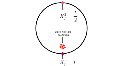
Figure 1: A sketch of a black-hole-like excitation created by the inhomogeneous quench in (1+1)d CFT on a ring, localized around the fixed point $X^{1}_{f}=0$.

The above behaviors, detected by the time evolution of the von Neumann entropy and the two-point correlation functions, are independent of the details of CFTs, i.e., holographic v.s. free fermion CFTs. We also study other quantities, such as mutual information defined for multiple subintervals.

For the case of holographic CFTs, we found gravity duals of these time-dependent states quenched by $H_{\theta}$ and $H_{\text{SSD}}$. From the behavior of this gravity duals, we found that the periodic behavior of the state quenched by $H_{\theta}$ is due to the periodic deformation of the black hole horizon. In contrast, when quenched by $H_{{\text{SSD}}}$, the black-hole horizon does not oscillate, but undergoes a deformation such that it asymptotically approaches and “touches” the boundary as $t\to\infty$, to create the black-hole-like excitation at the origin.

1.3 Organization

The rest of the paper is organized as follows: In Sec. 2, we start our analysis by computing the density operator $\rho(t)$ and setting up the calculations of physical observables in the Heisenberg picture. In Sec. 3, we calculate the time-dependence of the von Neumann entropy for single intervals. We in particular identify a black-hole-like excitation that emerges at the origin by the SSD quench 3.3. The nature of the black-hole-like excitation is further studied in the subsequent sections. In Sec. 4, the expectation values of the energy-momentum tensor and energy current are studied. In Sec. 5, we construct the holographic description of the black-hole-like excitation. The black-hole-like excitation emerges as the horizon of the BTZ black hole approaches the boundary. Section 6 is devoted to the analysis of mutual information for two intervals. As the behaviors of mutual information is theory-dependent, we study the holographic and free fermion CFTs separately. In both cases, we confirm the late time approximation of the density matrix in (1.7). Furthermore, we also discuss a finer structure of the late time state beyond the approximation (1.7). Finally, in Sec. 7, we further discuss the properties of the black-hole-like excitation. In particular, we discuss possible experimental realizations using quantum simulators, connection to the measurement-induced transitions in monitored quantum circuits, simulation of formation and evaporation of a black hole using the black-hole-like excitation. We close by mentioning various future directions.

2 Time-evolution after Möbius and SSD quench in 2d CFT

The time-evolution of quantum systems can be followed by looking at either the density matrix itself or various observables. In this section, we initiate our study on the Möbius and SSD quenches by discussing the time-evolution both in the Schrödinger and Heisenberg pictures. First, in Sec. 2.1, we follow the time-evolution of the density matrix using the algebraic properties of the Möbius and SSD Hamiltonians. Alternatively, in Sec. 2.2, we discuss the Heisenberg picture where (primary) operators are time-evolved by the Möbius and SSD Hamiltonians. In later sections, we will use the Heisenberg picture to compute various quantities such as von Neumann entropy, energy density, energy current, two-point functions, and mutual information. We will come back to the Schrödinger picture in Sec. 5, where we discuss the holographic dual of the time-evolution of the density matrix.

2.1 The density matrix in the Schrödinger picture

Let us first calculate $\rho(t)=e^{-itH_{\theta}}\rho(0)e^{+itH_{\theta}}$ directly. To this end, we recall that the Möbius Hamiltonian is written in terms of the Virasoro generators $\{L_{0,\pm 1},\bar{L}_{0,\pm 1}\}$ as

$$H_{0} =\oint\frac{dw}{2i\pi}T(w)+\oint\frac{d\bar{w}}{2i\pi}\bar{T}(\bar{w})=\frac{2\pi}{L}\left(L_{0}+\bar{L}_{0}\right)-\frac{\pi c}{6L},$$

$$H_{\pm} =\oint\frac{dw}{2i\pi}e^{\pm\frac{2\pi w}{L}}T(w)+\oint\frac{d\bar{w}}{2i\pi}e^{\mp\frac{2\pi\bar{w}}{L}}\bar{T}(\bar{w})=\frac{2\pi}{L}(L_{\pm 1}+\bar{L}_{\pm 1}),$$ (2.1)

where we introduce the complex coordinates, $w=\tau+ix$ and $\bar{w}=\tau-ix$, with $\tau$ and $x$ coordinatizing the (Euclidian) temporal and spatial directions, respectively, and $T(w)$ and $\bar{T}(\bar{w})$ are the holomorphic and anti-holomorphic parts of the energy-momentum tensor. These generators form the ${\it sl}(2,\mathbb{R})$ algebra,

$$X=L_{0},\quad Y=\frac{1}{2}(L_{-1}-L_{+1}),\quad Z=\frac{1}{2}(L_{-1}+L_{+1}),$$

$$[X,Y]=Z,\quad[X,Z]=Y,\quad[Z,Y]=X.$$ (2.2)

This algebraic structure allows us to compute $\rho(t)=e^{-itH_{\theta}}\rho(0)e^{+itH_{\theta}}$ explicitly. For the presentational simplicity, let us focus on the holomorphic sector only. Then, for the Möbius Hamiltonian $H_{\theta}=(2\pi/L)(X-c/24)-\tanh(2\theta)(2\pi/L)Z$, it is straight forward to show

$$\tilde{X} =e^{-itH_{\theta}}Xe^{+itH_{\theta}}$$

$$=\left[\cosh^{2}(2\theta)-\sinh^{2}(2\theta)\cos(\Omega t)\right]X$$

$$\quad-\cosh(2\theta)\sinh(2\theta)[1-\cos(\Omega t)]Z-\sinh(2\theta)\sin(\Omega t)iY.$$ (2.3)

(See [85] for a similar calculation.)

Thus, the state oscillates with the frequency $\Omega$ defined in (1.6). The oscillatory behavior after the Möbius quench can be understood from the discrete energy spectrum of the Möbius Hamiltonian [47, 48]. The Möbius Hamiltonian, in a proper coordinate system $z,\bar{z}$, can be written down by the Virasoro generator as $H_{\theta}=\Omega\big{(}L_{0}^{\tilde{z}}+\bar{L}_{0}^{\overline{\tilde{z}}}\big{)}-\frac{c\pi}{6L}.$ The “regularity” or “integrability” of the energy spectrum within each tower of states is responsible for the oscillation: The matrix elements of the density matrix in terms of the eigenstates $\left|n\right>_{\theta}$ of the Möbius Hamiltonian, $\rho_{mn}(t)=\left<m\right|_{\theta}\rho(t)\left|n\right>_{\theta}=e^{it(E_{m}-E_{n})}\left<m\right|_{\theta}\rho(0)\left|n\right>_{\theta}$, are periodic in time within each tower of states, since the energy difference $E_{m}-E_{n}$ is an integer multiple of $\Omega$. The periodicity of the oscillation is set by $2\pi/\Omega$ [86, 87, 88]. In the later sections, we will investigate this oscillation more closely.

On the other hand, since the system size is effectively infinite in the SSD limit, the periodic behavior does not occur. Taking the SSD limit $\theta\to+\infty$ in (2.1),

$$\cosh^{2}(2\theta)-\sinh^{2}(2\theta)\cos(\Omega t)\to 1+2\pi^{2}t^{2}/L^{2},$$

$$-\cosh(2\theta)\sinh(2\theta)[1-\cos(\Omega t)]\to-2\pi^{2}t^{2}/L^{2},$$

$$-\sinh(2\theta)\sin(\Omega t)\to-i2\pi t/L.$$ (2.5)

Further taking the limit $t\to\infty$, $e^{-itH_{\mathrm{SSD}}}H_{0}e^{+itH_{\mathrm{SSD}}}\sim\frac{2\pi^{2}t^{2}}{L^{2}}H_{\mathrm{SSD}}+{\it const}.$ We then conclude at late times, $\rho(t)$ would be given by $\rho(t)\sim e^{-(\epsilon 2\pi^{2}t^{2}/L^{2})H_{\mathrm{SSD}}}.$ Since the ground state of $H_{\mathrm{SSD}}$ is the same as the ground state of $H_{0}$, at late enough times, we expect $\rho(t)$ would be approximated by the ground state of $H_{0}$. In the next section, we will confirm this expectation by studying the von Neumann entropy defined for single intervals. When the intervals do not include $x=0$, we will see that the von Neumann entropy at late enough times is given by entanglement entropy of the ground state.

On the other hand, when the interval includes $x=0$, we will see that the von Neumann entropy is not given by the ground state value, but by the total thermal entropy (once again at late enough times); the above expectation $\rho(t)\sim e^{-(\epsilon 2\pi^{2}t^{2}/L^{2})H_{\mathrm{SSD}}}$ breaks down around the origin $x=0$. We defer the detailed discussion for later sections. However, we note that taking the $t\to\infty$ limit is somewhat subtle around the origin $x=0$. We go back to (2.1), and look at the transformed $X$ more closely. Recalling $(2\pi/L)L_{\pm}=\int dxe^{i2\pi x/L}h(x)$, where $h(x)$ is the Hamiltonian density, $\tilde{X}$ can be written as $\tilde{X}=\int dx\,\tilde{f}(x)h(x),$ with the envelope function given by

$$\tilde{f}(x) =\frac{\pi}{L}\Big{[}1+\cosh(4\theta)-\sinh(4\theta)\cos\left(\frac{2\pi x}{L}\right)[1-\cos(\Omega t)]$$

$$\quad\quad-2\sinh^{2}(2\theta)\cos(\Omega t)-2\sinh(2\theta)\sin\left(\frac{2\pi x}{L}\right)\sin(\Omega t)\Big{]}$$ (2.6)

For a given $x$, the envelop function in the SSD limit is given by

$$\tilde{f}(x)\to\frac{2\pi}{L}\left\{1-\frac{2\pi t}{L}\sin\left(\frac{2\pi x}{L}\right)+\frac{2\pi^{2}t^{2}}{L^{2}}\left[1-\cos\left(\frac{2\pi x}{L}\right)\right]\right\}.$$ (2.7)

For generic $x\neq 0$, the envelop function is quadratic in $t^{2}$, in agreement with the discussion above. On the other hand, for $x=0$, $f(x=0)\to\frac{2\pi}{L}$ and hence we do not have $t^{2}$ dependence at late times. This indicates that the density operator $\rho(t)$ near the origin should not be approximated as $e^{-(\epsilon 2\pi^{2}t^{2}/L^{2})H_{\mathrm{SSD}}}$.

2.2 Observables in the Heisenberg picture

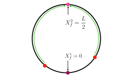
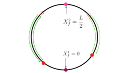
(a) The SSD time evolution (b) The Möbius time evolution

Figure 2: A sketch of how the spatial locations of an operator evolve in the Heisenberg picture for (a) the SSD and (b) Möbius time evolutions. The initial insertion points of the operator are marked by red. The two fixed points $X^{1}_{f}=0$ and $X^{2}_{f}=L/2$ are marked by purple.

Instead of the following the time-dependence of the density matrix $\rho(t)$, the time-dependence of correlation functions $\mathrm{Tr}\,\left[\mathcal{O}_{1}(X_{1})\mathcal{O}_{2}(X_{2})\cdots\rho(t)\right]$ can be followed by using the Heisenberg picture,

$$\mathcal{O}_{i}(X,t)=e^{+\epsilon H_{0}}e^{-itH_{\theta}}\mathcal{O}_{i}(X)e^{+itH_{\theta}}e^{-\epsilon H_{0}}.$$ (2.8)

Here, $\mathcal{O}_{i}(X)$ is a (primary) operator located at $X$ on the circle. For a primary operator $\mathcal{O}$ at $X$ with conformal dimension $(h,\bar{h})$, its Heisenberg evolution can be computed explicitly as

$$e^{\epsilon H_{0}}e^{itH_{\theta}}\mathcal{O}(w_{X},\bar{w}_{X})e^{-itH_{\theta}}e^{-\epsilon H_{0}}=\left(\frac{dw_{X}^{\text{new}}}{dw_{X}}\right)^{h}\left(\frac{d\bar{w}_{X}^{\text{new}}}{d\bar{w}_{X}}\right)^{\bar{h}}\mathcal{O}(w^{\text{new}}_{X},\bar{w}_{X}^{\text{new}}),$$ (2.9)

where $w_{X}=iX,\bar{w}_{X}=-iX$, and $w^{\text{new}}_{X}$ and $\bar{w}^{\text{new}}_{X}$ are given by

$$w^{\text{new}}_{X}=\frac{L}{2\pi}\log{\left(\lambda_{0}\left[\frac{[(1-\lambda)\cosh{(2\theta)-(\lambda+1)}]z+(\lambda-1)\sinh{(2\theta)}}{(1-\lambda)\sinh{(2\theta)}z+[(\lambda-1)\cosh{(2\theta)}-(\lambda+1)]}\right]\right)},$$ (2.10)

$$\bar{w}^{\text{new}}_{X}=\frac{L}{2\pi}\log{\left(\lambda_{0}\left[\frac{[(1-\lambda)\cosh{(2\theta)-(\lambda+1)}]\bar{z}+(\lambda-1)\sinh{(2\theta)}}{(1-\lambda)\sinh{(2\theta)}\bar{z}+[(\lambda-1)\cosh{(2\theta)}-(\lambda+1)]}\right]\right)},$$ (2.11)

where $z=e^{\frac{2\pi w}{L}}$, $\bar{z}=e^{\frac{2\pi\bar{w}}{L}}$, $\lambda_{0}=e^{\frac{2\pi\epsilon}{L}}$, and $\lambda=e^{i\Omega t}$. In the SSD limit, from the leading order contributions in the large $\theta$ expansion,

$$\begin{split}&w^{\text{new}}_{X}\underset{\theta\rightarrow\infty}{\approx}\frac{L}{2\pi}\log{\left(\lambda_{0}\left[\frac{i\pi(1-z)t-Lz}{i\pi(1-z)t-L}\right]\right)},\\ &\bar{w}^{\text{new}}_{X}\underset{\theta\rightarrow\infty}{\approx}\frac{L}{2\pi}\log{\left(\lambda_{0}\left[\frac{i\pi(1-\bar{z})t-L\bar{z}}{i\pi(1-\bar{z})t-L}\right]\right)}.\end{split}$$ (2.12)

Denoting the real and imaginary parts of $w^{\text{new}}_{X},\bar{w}^{\text{new}}_{X}$ as $w^{\text{new}}_{X}=\epsilon+i\varphi L/\pi$, $\bar{w}^{\text{new}}_{X}=\epsilon+i\bar{\varphi}L/\pi$ ($-\pi\leq-\varphi,\bar{\varphi}\leq 0$), the spatial and temporal locations, $X^{\text{new}}$, $\tau^{\text{new}}$, of the transformed operator can be identified as

$$X^{\text{new}} =\frac{w_{X}^{\text{new}}-\bar{w}_{X}^{\text{new}}}{2i}=\frac{L(\varphi-\bar{\varphi})}{2\pi},$$ (2.13)

$$\tau^{\text{new}} =\frac{w_{X}^{\text{new}}+\bar{w}_{X}^{\text{new}}}{2}=\epsilon+i\frac{L\left(\varphi+\bar{\varphi}\right)}{2\pi}.$$ (2.14)

(See Appendix A for details.) In this coordinate system, $\tau^{\text{new}}$ is a complex function of $X_{i}$ and $t$, while $X^{\text{new}}$ is a real function of $X_{i}$ and $t$. The time evolution operator moves the operator along the spatial and imaginary time directions $X^{\text{new}}$ and $\tau^{\text{new}}$.

There are two fixed points that are left invariant under the Möbius and SSD evolutions:

$$X^{1}_{f}=0,\qquad X^{2}_{f}=\frac{L}{2}.$$ (2.15)

For the Möbius evolution, if an operator is inserted at a point other than the fixed points, $X^{\text{new}}$ and $\tau^{\text{new}}$ undergo periodic motion with period $2\pi/\Omega$. (Fig. 2(b)). For the SSD evolution, and operators inserted at other points than $X^{1}_{f}$ flow to $X^{2}_{f}$ (Fig. 2(a)).

3 Von Neumann entropy for single intervals

The von Neumann entropy for a given subsystem $A$, $S_{A}=\lim_{n\rightarrow 1}\frac{1}{1-n}\log{\left[\mathrm{Tr}_{A}\left(\rho_{A}\right)^{n}\right]}$, can be calculated by using the twist operator formalism [89, 90]. For a single interval $[X_{1},X_{2}]$,

$$\begin{split}S_{A}=\lim_{n\rightarrow 1}\frac{1}{1-n}\log{\left\langle\mathcal{T}_{n}(w_{X_{1}},\bar{w}_{X_{1}})\bar{\mathcal{T}}_{n}(w_{X_{2}},\bar{w}_{X_{2}})\right\rangle},\end{split}$$ (3.1)

where $\mathcal{T}_{n}$ and $\bar{\mathcal{T}}_{n}$ are the twist and anti-twist operators in the Heisenberg picture, (2.8). In terms of the original twist and anti-twist operators $S_{A}$ is given by [58, 59, 61, 63],

$$\begin{split}S_{A}&=-\frac{c}{12}\log{\left[\Pi_{i=1,2}\left(\frac{dw_{X_{i}}^{\text{new}}}{dw_{X_{i}}}\frac{d\bar{w}_{X_{i}}^{\text{new}}}{dw_{X_{i}}}\right)\right]}\\ &\quad+\lim_{n\rightarrow 1}\frac{1}{1-n}\log{\left[\left\langle\mathcal{T}_{n}(w^{\text{new}}_{X_{1}},\bar{w}^{\text{new}}_{X_{1}})\bar{\mathcal{T}}_{n}(w^{\text{new}}_{X_{2}},\bar{w}^{\text{new}}_{X_{2}})\right\rangle_{2\epsilon}\right]},\end{split}$$ (3.2)

where the last term of (3.2) is given as the von Neumann entropy of a thermal state at inverse temperature $2\epsilon$ on a compact spacetime. We note that, since $w_{X_{i}}^{\text{new}}$ and $\bar{w}_{X_{i}}^{\text{new}}$ vary in time in the Heisenberg picture, the subsystem size varies in the Möbius/SSD time evolution.

Since there is no translation symmetry in our inhomogeneous quenches, the von Neumann entropy $S_{A}$ depends not only on the size of the subsystem $A$ but also on the location of $A$. In the following, we will work with the following three choices of the subsystem $A$:

$$\begin{split}A=\begin{cases}\left\{x\big{|}0\leq x\leq X,L-X\leq x\leq L\right\}&\text{Case 1}\\ \left\{x\big{|}\frac{L}{4}-X\leq x\leq\frac{L}{4}+X\right\}&\text{Case 2}\\ \left\{x\big{|}\frac{L}{2}-X\leq x\leq\frac{L}{2}+X\right\}&\text{Case 3}\\ \end{cases}.\end{split}$$ (3.3)

In Case 1, the center of the subsystem $A$ is $X^{1}_{f}$, one of the fixed points, and in Case 3 the center is the other fixed point $X^{2}_{f}$. In Case 2, the center of the subsystem $A$ is the midpoint between $X^{1}_{f}$ and $X^{2}_{f}$.

We will study both a CFT with a gravity dual (holographic CFT) and a free fermion CFT. However, for the von Neumann entropy for a single interval, there is essentially no difference between these two cases. We therefore focus on the holographic CFT here. On the other hand, mutual information defined for two (disjoint) intervals probes the details of CFTs, as we will see in Sec. 6. In holographic CFTs, in the coarse-grained limit, i.e., the limit where all parameters are sufficiently larger than $\epsilon$, the final term in (3.2) can be computed from the gravity dual which is the BTZ black hole [91]. As in [92, 93], it is given by

$$\begin{split}&\lim_{n\rightarrow 1}\frac{1}{1-n}\log{\left\langle\mathcal{T}_{n}(w^{\text{new}}_{X_{1}},\bar{w}^{\text{new}}_{X_{1}})\bar{\mathcal{T}}_{n}(w^{\text{new}}_{X_{2}},\bar{w}^{\text{new}}_{X_{2}})\right\rangle_{2\epsilon}}\\ &\approx\frac{c}{3}\log{\left(\frac{2\epsilon}{\pi}\right)}\\ &\quad+\left\{\begin{array}[]{l}\text{Min}\bigg{[}\frac{c}{6}\log{\left|\sin{\left[\frac{\pi}{2\epsilon}(w^{\text{new}}_{X_{1}}-w^{\text{new}}_{X_{2}})\right]}\right|^{2}},\frac{c\pi L}{6\epsilon}+\frac{c}{6}\log{\left|\sin{\left[\frac{\pi}{2\epsilon}(w^{\text{new}}_{X_{1}}-w^{\text{new}}_{X_{2}}\pm iL)\right]}\right|^{2}}\bigg{]}\\ \qquad\qquad\qquad\text{for Case 1}\\ \text{Min}\bigg{[}\frac{c\pi L}{6\epsilon}+\frac{c}{6}\log{\left|\sin{\left[\frac{\pi}{2\epsilon}(w^{\text{new}}_{X_{1}}-w^{\text{new}}_{X_{2}})\right]}\right|^{2}},\frac{c}{6}\log{\left|\sin{\left[\frac{\pi}{2\epsilon}(w^{\text{new}}_{X_{1}}-w^{\text{new}}_{X_{2}}\pm iL)\right]}\right|^{2}}\bigg{]}\\ \qquad\qquad\qquad\text{for Case 2 and 3}\end{array}\right.\end{split}$$ (3.4)

Here, $\frac{c\pi L}{6\epsilon}$ is the entropy of the black hole, i.e., the thermal entropy, and all lengths are measured in the unit of some UV cutoff (lattice spacing).

3.1 The Möbius quench

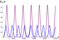
(a) $S_{A}$ for Case 1.
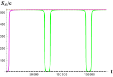
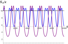
(b) $S_{A}$ for Case 2.
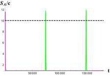
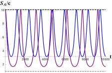
(c) $S_{A}$ for Case 3.

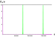
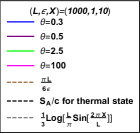
Figure 3: The time evolution of von Neumann entropy after the Möbius quench for the subsystems centered around (a) $x=X^{1}_{f}$, (b) $x=\frac{L}{4}$, and (c) $x=X^{2}_{f}$. The plots on the left show the early time evolution of the von Neumann entropy when $\theta\leq 0.5$.

Let us first study the Möbius quench with $\theta<\infty$ (Fig. 3). We find that, in all cases, the von Neumann entropy oscillates in time with the periodicity ${2\pi}/{\Omega}=L\cosh{(2\theta)}$, starting from the that of the thermal state $S_{A}(t=0)\approx{c\pi X}/{3\epsilon}$, in agreement with the discussion in Sec. 2.1. When $\theta$ is sufficiently large, in Case 1, the von Neumann entropy oscillates between the initial value ${c\pi X}/{3\epsilon}$ and the total thermal entropy $S_{\text{thermal}}={c\pi L}/{6\epsilon}$. On the other hand, in Case 3 where the subsystem is centered around $X^{2}_{f}$ (and once again when $\theta$ is sufficiently large), the von Neumann entropy oscillates between the initial value ${c\pi X}/{3\epsilon}$ and the ground state value $(c/3)\log[(L/\pi)\sin(2\pi X/L)]$. See Fig. 3 for other cases.

3.2 The SSD quench

(a) $S_{A}$ for Case 1	(b) $S_{A}$ for Case 2
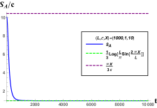
(c) $S_{A}$ for Case 3	(d) Size dependence of von Neumann entropy in Case 1

Figure 4: The time evolution of the von-Neumann entropy entropy after the SSD quench for the subsystems centered around (a) $x=X^{1}_{f}$, (b) $x=\frac{L}{4}$, and (c) $x=X^{2}_{f}$. (d) The subsystem size dependence of $S_{A}(t)$ in Case 1.

Let us now move on to the SSD limit. The main difference from the Möbius quench is the absence of oscillations in the SSD quench. Plotted in Fig. 4(a) is the time evolution of $S_{A}$ for the setup of Case 1 in the SSD limit. Initially, $S_{A}$ is given by the von Neumann entropy of the thermal state,

$$S_{A}(t\approx 0)\approx\frac{c\pi X}{3\epsilon},$$ (3.5)

where $2X$ is the size of the subsystem. As time goes by, $S_{A}$ increases in time. For a sufficiently late time $t>t_{*}$, where $t_{*}$ is some characteristic time, $S_{A}$ can be approximated by the thermal entropy of the total system:

$$S_{A}(t\gg t_{*})\approx\frac{c\pi L}{6\epsilon}=S_{\text{thermal}},$$ (3.6)

which is independent of the subsystem size. The characteristic time $t_{*}$ can be estimated by using the quasiparticle picture, or by directly inspecting the holographic result. Either way, if the size of the subsystem is sufficiently small, $\epsilon\ll 2X\ll L$, $t_{*}$ is inversely proportional to the subsystem size $2X$, and given by

$$t_{*}\approx\frac{L^{2}}{2\pi^{2}X}.$$ (3.7)

We defer the details of the quasiparticle picture and estimation of $t_{*}$ to a later section. These behaviors can be understood from the evolution of the minimal surface (geodesic) in the Heisenberg picture (Fig. 5(a)). At late times, the geodesic encloses the black hole.

In Case 2, the von Neumann entropy initially increases with time, reaches a maximum, and then decreases (Fig. 4(b)). On the other hand, in Case 3 the von Neumann entropy decreases monotonically (Fig. 4(c)), since the geodesic becomes smaller with time (Fig. 5[b]). In both cases, the von Neumann entropy asymptotically approaches the vacuum entanglement entropy [89, 90] after a sufficient time has passed:

$$S_{A}(t\rightarrow\infty)\approx\frac{c}{3}\log{\left[\frac{L}{\pi}\sin{\left(\frac{2\pi X}{L}\right)}\right]}.$$ (3.8)

The von Neumann entropy, for the cases when the subsystem does not contain $x=X^{1}_{f}$, thus undergoes a crossover from the volume-law to area-law entanglement entropy.

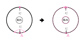
(a) Geodesic in case 1.

(b) Geodesic in case 3.

Figure 5: The time evolution of the geodesic in the Heisenberg picture for Case 1 (Left) and Case 3 (Right). In Case 1, we note that due to the homology condition of the holographic entanglement entropy the geodesic encircles the black hole at late times.

3.3 Black-hole-like excitation

To summarize, when $A$ is centered around the fixed point $x=X^{1}_{f}$, $S_{A}(t)$ saturates to $S_{\text{thermal}}=S_{\text{B.H.}}$, which does not depend on the subsystem size, while when the subsystem $A$ does not include the fixed point $x=X^{1}_{f}$, at late enough times, $S_{A}(t)$ is well approximated by the entanglement entropy of the vacuum state. These indicate that, at late enough times, almost all quantum degrees of freedom (entropy) are concentrated at the fixed point $x=X^{1}_{f}$: At the fixed point $x=X^{1}_{f}$, a local excitation with as much information as compatible with thermal entropy emerges (Fig. 1). To be more precise, in the coarse-grained limit (in the limit of $\epsilon\ll 1$), the difference between the physical quantity for the exact density operator and that for the approximated density operator in (1.7) is at most $\mathcal{O}(1)$. In the SSD dynamics, from the point of view of a subsystem containing a fixed point $x=X^{1}_{f}$, the degrees of freedom (quasi-particles, which we will explain later) of the system gather at the fixed point at a position-dependent rate. Here, we assume that the spatial size of this excitation is about $\mathcal{O}(\epsilon)$, and its center of mass is $x=X^{1}_{f}$. The high entropy state at the fixed point is “holographic” in the sense that the subsystem can be effectively viewed as a small $0$-dimensional point from the perspective of the whole system; while the total system is one-dimensional, the entropy comes from a zero-dimensional point. Effectively, the system is reduced to a point [94, 95]. This behavior is reminiscent of a black hole: In quantum gravity theory, in the low-energy limit, almost all the degrees of freedom are localized on the surface of a black hole [96, 97, 98]. Because of this similarity, we call the excitations concentrated at $x=X^{1}_{f}$ a black-hole-like excitation. After this black-hole-like excitation emerges at $x=X^{1}_{f}$, the von Neumann entropy is well approximated by (1.7).

We argue that by the SSD quench we can simulate the formation process of black holes in which the black-hole-like excitation emerges. The analogy between the high entropy state at the fixed point and a black hole can be sharpened in holographic CFTs. As we will see in Sec.  5, in the holographic theory, the SSD quench deforms the bulk black hole horizon such that at late times, the bulk horizon “touches” the boundary at the fixed point. Thus, the black-hole-like excitation can be identified with the horizon.

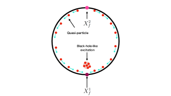
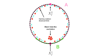
[a] Formation [b] Evaporation

Figure 6: Formation [a] and evaporation [b] of a black-hole-like excitation.

3.4 The quasi-particle picture

The above findings on the entanglement dynamics can be explained by an effective model of entanglement propagation, the quasi-particle picture, as we discuss below. In particular, we apply the approach discussed in [23, 99], where the quasiparticle picture was generalized from homogeneous to inhomogeneous quenches [60, 63].

The quasi-particle picture describes the time evolution of the leading contribution of the von Neumann entropy in the coarse-graining limit, i.e., the contributions of order $\mathcal{O}\left({1}/{\epsilon}\right)$, where $\epsilon$ is the UV cutoff (lattice spacing). At $t=0$, we assume that there are a pair of quasiparticles at each lattice site. Suppose that the von Neumann entropy of a subsystem $A$ is proportional to the number of quasiparticles in the subsystem $A$. For the initial state, $S_{A}$ is given by $S_{A}\approx\mathcal{N}\cdot{l}/{\epsilon},$ where $l$ is the subsystem size, and $\mathcal{N}$ is a constant. After the SSD quench, the quasiparticles in $X^{2}_{f}\geq x\geq X^{1}_{f}$ propagate from $X^{2}_{f}$ to $X^{1}_{f}$, while those in $L\geq x>X^{2}_{f}$ propagate from $X^{2}_{f}$ to $x=L$. The velocity $v(x)$ of these quasiparticles is position dependent and can be read off from the envelope function of the energy density [60, 63],

$$H=\int^{L}_{0}\frac{dx}{2\pi}\left[v(x)T(w)+\bar{v}(x)\bar{T}(\bar{w})\right].$$ (3.9)

In particular, for the SSD quench,

$$v(x)=\bar{v}(x)=2\sin^{2}{\left(\frac{\pi x}{L}\right)}.$$ (3.10)

Namely, the speed of propagation increases monotonically for $X_{f}^{1}<x<X_{f}^{2}$, takes a maximum value at $x=X_{f}^{2}$, then decreases monotonically for $X_{f}^{1}<x<L$, and has a minimum value at $x=L$. The maximum and minimum values, respectively, are given by

$$v_{\text{max}}=v(x=X_{f}^{2})=2,\quad v_{\text{min}}=v(x=X_{f}^{1},L)=0.$$ (3.11)

Case 1

Let us now apply the quasiparticle picture to describe the entanglement dynamics in Case 1. Since the von Neumann entropy in Case 1 is $\mathcal{O}\left({1}/{\epsilon}\right)$, we expect the quasiparticle picture can describe its time evolution. The time at which the von Neumann entropy can be approximated by thermal entropy, $t^{\mathrm{SSD}}_{p}$, can be estimated by the time at which all quasiparticles in $L-X\leq x\leq X$ enter the subsystem $A$, and given by

$$t^{\mathrm{SSD}}_{p}=\int^{\frac{L}{2}}_{X}\frac{dx}{2\sin^{2}{\left(\frac{\pi x}{L}\right)}}=\frac{L}{2\pi}\cot{\left(\frac{\pi X}{L}\right)}.$$ (3.12)

This accurately reproduces the crossover observed in Fig. 4(d).

Alternatively, the characteristic time $t_{*}$, the approximate time at which the von Neumann entropy becomes the thermal entropy, can be estimated by the time when the distance between the twist and anti-twist operators is sufficiently small in the Heisenberg picture. To be more precise, we define $t_{*}$ from $\cos{\left[\varphi_{L-X}-\varphi_{X}-\left(\bar{\varphi}_{L-X}-\bar{\varphi}_{X}\right)\right]}\approx 1$ and $\sin{\left[\varphi_{L-X}-\varphi_{X}-\left(\bar{\varphi}_{L-X}-\bar{\varphi}_{X}\right)\right]}\approx 0$:

$$t_{*}=\frac{L}{2\pi}\sqrt{\cot^{2}{\left(\frac{\pi X}{L}\right)}-1}.$$ (3.13)

If the size of the system is sufficiently large, $\epsilon\ll X\ll L$, the two values coincide and are given by (3.7), $t_{*}=t^{\text{SSD}}_{p}\approx{L^{2}}/{2\pi^{2}X}$. Even when the center of the subsystem is not at $X_{f}^{1}$, the quasi-particle picture can still be used to describe the time evolution of the von Neumann entropy (see Appendix B).

Case 2 and 3

For Case 2 and 3, where the subsystem does not include $X^{1}_{f}$, it is expected that the dynamics of the von Neumann entropy is not explained by the quasiparticle picture at late times. This is because the volume to area-law crossover occurs, after which the von Neumann entropy becomes $\mathcal{O}(1)$. Within the quasiparticle picture, the crossover time is estimated by the time at which the number of quasiparticles in the subsystem $A$ becomes zero. It is given by $t_{\text{Case}~{}2}\approx\frac{L}{2\pi}\cot{\left(\frac{\pi}{4}-\frac{\pi X}{L}\right)}$ and $t_{\text{Case}~{}3}\approx\frac{L}{2\pi}\tan{\left(\frac{\pi X}{L}\right)}$ for Case 2 and 3, respectively. Since $A$ is sufficiently small compared to $B$, it is expected that in Case 2 and 3, the quasiparticle picture breaks down when $t\geq t_{\text{Case}~{}i=2,3}$ and an alternative description is needed. A more accurate estimate of the crossover time is given by

$$t_{\text{volume-area}}\approx\frac{L}{2\pi}\cdot\sqrt{\frac{L}{2\epsilon}\left|\cot{\left(\frac{\pi X}{L}\right)}-\cot{\left(\frac{\pi Y}{L}\right)}\right|}.$$ (3.14)

Here, the subsystem $A$ is assumed to be $A=\{x|L>X>x>Y>0\}$.

Nevertheless, we can still use the quasiparticle picture to discuss earlier times, in particular the peak structure observed in Case 2. Since the closer to $x=X_{f}^{2}$, the larger the velocity of the quasiparticles, we expect that the number of quasiparticles flowing into the subsystem $A$ is initially larger than those flowing out in Case 2. The peak appears when the numbers of quasiparticles flowing in and out the subsystem $A$ are balanced. For simplicity, however, let us approximate the time of the peak by the time when all the quasiparticles on $\frac{L}{4}+X<x<X^{2}_{f}$ enter the subsystem. Under this assumption, the time when the peak appears, $t_{\text{peak}}$, is estimated as

$$t_{\text{peak}}\approx\frac{L}{2\pi}\cot{\left(\frac{\pi}{4}+\frac{\pi X}{L}\right)}.$$ (3.15)

This estimation is more accurate for larger $L/X$. This is because the number of outflowing and inflowing quasiparticles are more balanced when the size of the subsystem is small in a system where the velocity depends on the position.

4 Energy-momentum tensor and energy current

The time-evolution of the von Neumann entropy studied in the previous section suggests that under the SSD quench a black-hole-like excitation propagates and localizes at the origin at late times. In this section, we examine the expectation value of the energy-momentum tensor and local energy current to probe the dynamics of the black-hole-like excitation. The energy-momentum tensor profile is also useful for studying the holographic dual of the SSD/Möbius quench (Sec. 5).

The transformation law of the energy-momentum tensor under SSD/Möbius deformation is the same as that of local operators discussed in (2.9), except for the contribution from the Schwarzian derivative. For the holomorphic part, it is given by

$$T^{\theta}(w) \equiv e^{iH_{\theta}t}T(w)e^{-iH_{\theta}t}$$

$$=\left(\dfrac{dw^{\textrm{new}}_{X}(w)}{dw}\right)^{2}T(w^{\textrm{new}}_{X})+\dfrac{c}{12}\mathrm{Sch}(w^{\textrm{new}}_{X}(w),w).$$ (4.1)

where $w=iX$ (see around Eq. (2.9)) and we define the Schwarzian derivative as

$$\mathrm{Sch}(f(w),w)=\dfrac{f^{\prime\prime\prime}(w)}{f^{\prime}(w)}-\dfrac{3}{2}\left(\dfrac{f^{\prime\prime}(w)}{f^{\prime}(w)}\right)^{2}.$$ (4.2)

The Schwarzian term is a consequence of the Weyl anomaly and explains the contribution from the Casimir energy.

4.1 Pure state approximation

It is well known that the expectation value of the energy-momentum tensor for high-energy eigenstates can be well approximated by the expectation value for thermal states. Based on this fact, instead of the thermal state itself, we first estimate the expectation value of the energy-momentum tensor for a high-energy eigenstate without angular momentum. We will later confirm that this approximation precisely reproduces the time-dependent part of the energy-momentum tensor of the free fermion CFT, which will be derived without approximation.

The SSD quench

In the SSD quench, we have

$$T^{\textrm{SSD}}(X,t) \equiv\langle\psi_{{\cal O}_{h}}|T^{\theta\to\infty}(w)|\psi_{{\cal O}_{h}}\rangle$$

$$=\left(\dfrac{2\pi}{L}\right)^{2}\left[\dfrac{4h}{\left(\left(\frac{2\pi t}{L}\right)^{2}\left(1-\cos\left(\frac{2\pi}{L}X\right)\right)-2\left(\frac{2\pi t}{L}\right)\sin\left(\frac{2\pi}{L}X\right)+2\right)^{2}}-\dfrac{c}{24}\right].$$ (4.3)

The second term comes from the Casimir energy. Here we introduced $|\psi_{{\cal O}_{h}}\rangle$ as a spinless primary state with the conformal dimension $h_{L}=h_{R}=h$. Namely, the total energy at $t=0$ is given by $\frac{4\pi h}{L}$ up to the Casimir energy. We can also obtain $\langle\psi_{{\cal O}_{h}}|\bar{T}^{\theta\to\infty}(\bar{w})|\psi_{{\cal O}_{h}}\rangle$ by exchanging $X\rightarrow-X$. Note that one can relate the energy with (inverse) temperature $\beta$ by using the relation (see [100], for example),

$$\dfrac{h}{L^{2}}=\dfrac{c}{24\beta^{2}}.$$ (4.4)

We plot the energy-momentum tensor profile Eq. (4.3) in Fig. 7.

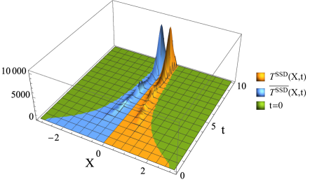
Figure 7: The holomorphic (orange) and anti-holomorphic (blue) parts of the energy-momentum tensor. The sum of these two parts gives the local energy density, while the difference gives a local energy current. In this figure, we set $L=2\pi$, and $c=\beta=1$. Also plotted are their initial values (green). These two peaks are both converging to a fixed point of the SSD quench, $X=X^{1}_{f}=0$.

We can see that both holomorphic and anti-holomorphic energy-momentum tensors are gathered towards the fixed point of the SSD transformation. Similarly, we obtain a local energy current as

$$J^{\textrm{SSD}}(X,t) \equiv\langle\psi_{{\cal O}_{h}}|T^{\theta\to\infty}(w)-\bar{T}^{\theta\to\infty}(\bar{w})|\psi_{{\cal O}_{h}}\rangle$$

$$=\left(\dfrac{2\pi}{L}\right)^{2}\left[\dfrac{4h}{\left(\left(\frac{2\pi t}{L}\right)^{2}\left(1-\cos\left(\frac{2\pi}{L}X\right)\right)-2\left(\frac{2\pi t}{L}\right)\sin\left(\frac{2\pi}{L}X\right)+2\right)^{2}}-(X\rightarrow-X)\right].$$ (4.5)

If we set $X=X^{1}_{f}=0$, both holomorphic and anti-holomorphic energy-momentum tensor take a constant value, hence there are no local energy flow, i.e. $J^{\textrm{SSD}}(0,t)=0$.

The location where the energy-momentum tensor takes its maximum value at each fixed time is given by

$$X^{(T)}_{\textrm{max}}(t)=\left(\dfrac{L}{\pi}\right)\tan^{-1}\left(\dfrac{L}{2\pi t}\right)\underset{t\rightarrow\infty}{\longrightarrow}0,$$ (4.6)

which is obtained from $\partial_{t}T^{\textrm{SSD}}(X,t)=0$. We will compare this with the peak of the black hole horizon in the next section.

These results, along with ones for the von Neumann entropy, provide further evidence that there are local black-hole-like excitations that propagate towards the fixed point of the SSD Hamiltonian and account for the thermal entropy.

The Möbius quench

A similar analysis can be done for the Möbius quench with generic $\theta$. The energy-momentum tensor and the local energy current will be denoted by $T^{M}$ and $J^{M}$ respectively. As in the von Neumann entropy, the Möbius deformed energy-momentum tensor has the $2\pi/\Omega=L\cosh 2\theta$ periodicity. For this reason, the Möbius deformed local energy current also acquires the $\pi/\Omega$ anti-periodicity. We defer plots for $T^{M}$ and $J^{M}$ to the next section as these are identical to ones for the free fermion.

4.2 The free fermion CFT

The one-point correlation function of the energy-momentum tensor on a torus is given by a derivative of the logarithm of the partition function with respect to the modular parameter [101, 102]. For the $c=1$ free Dirac fermion theory, the partition function for spin-structure $\nu$ is $Z_{\nu}=\frac{1}{2}\left|\frac{\theta_{\nu}(\tau)}{\eta(\tau)}\right|^{2}$[103]. Therefore, the expectation value of the energy-momentum tensor for spin-structure $\nu$ is

$$\langle T(w_{X}^{\text{new}})\rangle_{\nu}=2i\pi\partial_{\tau}\ln\left|\frac{\theta_{\nu}(\tau)}{\eta(\tau)}\right|^{2}$$ (4.7)

Using the product representation of the elliptic theta function and the Dedekind eta functions, the expectation value is found to be

$$\langle T(w_{X}^{\text{new}})\rangle_{\nu}=\frac{\pi^{2}}{3}-16\pi^{2}(-1)^{\nu+1}\sum_{m=1}^{\infty}\frac{(m-\frac{1}{2})e^{2\pi i(m-\frac{1}{2})\tau}}{1+(-1)^{\nu+1}e^{2\pi i(m-\frac{1}{2})\tau}}$$ (4.8)

Since the imaginary part of the modular parameter $\text{Im}\tau=\frac{L}{2\epsilon}\gg 1$, the sum is negligible, so the expectation value of the energy-momentum tensor under a Möbius evolution is

$$\langle T^{\theta}(w)\rangle=\left(\frac{dw_{X}^{\text{new}}}{dw}\right)^{2}\frac{\pi^{2}}{3}+\frac{c}{12}\text{Sch}(w_{X}^{\text{new}},w).$$ (4.9)

The one-point function for the energy-momentum tensor on the torus depends only on the modular parameter so (4.7) is the same for the anti-holomorphic part. In fact, the anti-holomorphic coordinates have the exact same expression as the holomorphic coordinates with the replacement $w\rightarrow\bar{w}$. Therefore, $\bar{T}^{\theta}(\bar{w})$ can be obtained from $T^{\theta}(w)$ by making the replacement $X\rightarrow-X$.

Plots of the spatial profile of the expectation value of the energy-momentum tensor (4.9) as well as the energy current at various instances in time for the SSD and Möbius quenches are shown in Fig. 8 and 9, respectively.

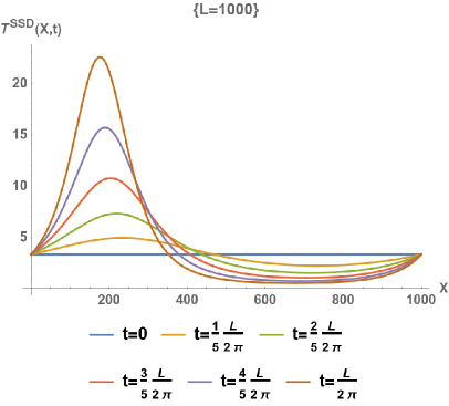
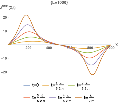
Figure 8: The spatial profile of the expectation value of the energy-momentum tensor (4.9) as well as the energy current at different times in the SSD limit for a total system size of $L=1000$.

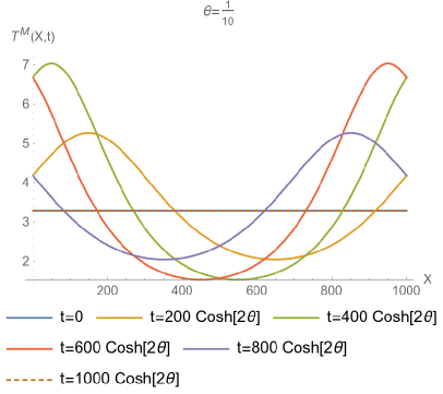
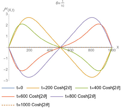
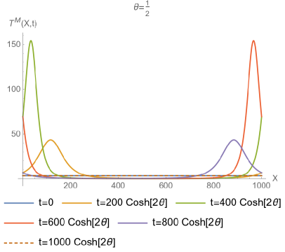
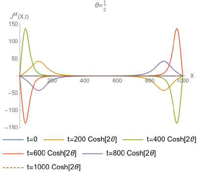
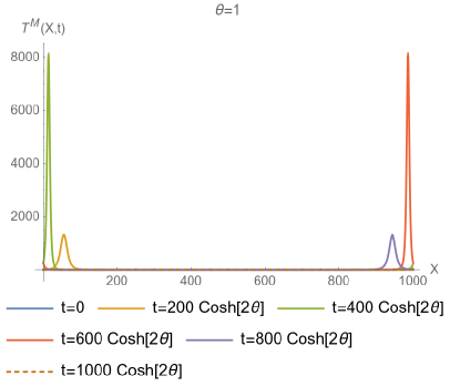
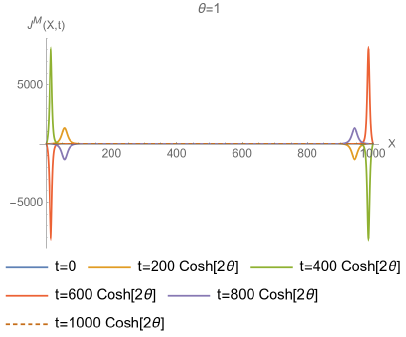
energy

Figure 9: Plots of the spatial profile of the energy-momentum tensor and heat current after a Möbius quench for $\theta=\frac{1}{10},\frac{1}{2},1$ at $t=0,\frac{L}{5}\cosh{2\theta},\frac{2L}{5}\cosh{2\theta},\frac{3L}{5}\cosh{2\theta},\frac{4L}{5}\cosh{2\theta},L\cosh{2\theta}$ with the total system size fixed at $L=1000$.

The spatial profiles for the energy-momentum tensor and the energy current for the Möbius and SSD quenches in the free fermion CFT are very similar to the pure state case. That is because the Schwarzian derivative in (4.9) turns out to be negligible compared to the conformal factor that comes from the Heisenberg evolution. The energy-momentum tensor is thus approximately determined by the first term in (4.9) where the conformal factor is theory-independent. The theory dependence only comes in through the one-point function of the energy-momentum tensor which is a time-independent quantity that only depends on the modular parameter of the torus. Therefore, the energy-momentum tensor for different CFTs differs only by a proportionality constant.

5 Bulk geometry in the Schrödinger picture

We have used the Heisenberg picture where the operators transformed under the Möbius/SSD quench while the state remained unchanged from the original thermal state. In this section, we discuss the Schrödinger picture where the state transforms under the inhomogeneous quench, and study the gravitational dual of the SSD-quenched state.

5.1 The SSD quench

As discussed in [104, 105], the gravitational dual can be constructed from the expectation value of the energy density after the quantum quench. This is equivalent to rewriting the geometry given by the static BTZ black hole in the $w^{\rm new}$ and $\bar{w}^{\rm new}$ coordinate system in terms of the original $X$ and time $t$ which parametrize the time evolution under the SSD Hamiltonian. The metric is given by

$$\begin{split}ds^{2}&=L^{2}\left[\frac{dr^{2}}{r^{2}-r_{0}^{2}}-\left(f_{tt,1}r^{2}-f_{tt,2}\frac{r_{0}^{2}}{4}\right)dt^{2}+\left(-f_{xx,1}r^{2}+f_{xx,2}\frac{r_{0}^{2}}{4}\right)dx^{2}+r^{2}_{0}f_{tx}dtdx\right].\\ \end{split}$$ (5.1)

The details of $f_{tt,i=1,2}$, $f_{xx,i=1,2}$, and $f_{tx}$ are given in Appendix C.1. We introduce a new radial coordinate $r^{\prime}=r\sqrt{-f_{xx,1}}$. The geometry asymptotically approaches

$$ds^{2}\approx L^{2}\left[\frac{dr^{\prime 2}}{r^{\prime 2}}+r^{\prime 2}\left[-4\sin^{4}{\left(\frac{\pi x}{L}\right)}dt^{2}+dx^{2}\right]\right]\,,$$ (5.2)

as $r^{\prime}\rightarrow\infty$, where the dual CFT lives. Notice that this boundary metric is sine-square deformed from the usual flat metric [106, 59]. Since the horizon sits at $r=r_{0}$, we identify the location of the horizon by

$$r^{\prime}_{\text{horizon}}=r_{0}\sqrt{-f_{xx,1}}$$ (5.3)

in the $r^{\prime}$ coordinate. The position of the horizon depends on the spatial coordinate $X$, and has a peak at

$$t=\frac{L\sqrt{1-4\sin^{2}\left(\frac{\pi X}{L}\right)}}{2\pi\sin\left(\frac{\pi X}{L}\right)}\,,$$ (5.4)

where $0<X<L/6,5L/6<X<L$. This is obtained by solving the equation $\partial_{X}r^{\prime}_{\rm horizon}=0$ with respect to $t$. See Fig. 10 for the plot of the profile of the horizon.

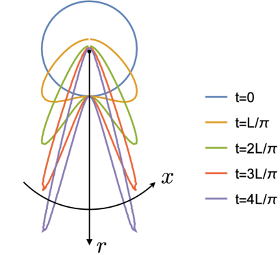
Figure 10: Time dependence of the horizon profile. Here we set $L=2\pi$.

By plugging this into (5.3), we obtain the $X$ dependence of the horizon at time (5.4)

$$r^{\prime}_{\text{horizon}}=\frac{r_{0}}{\left|\sin{\left(\frac{\pi X}{L}\right)}\right|}\,.$$ (5.5)

The position of the peak at time $t$ is given by

$$X=\frac{L}{\pi}\tan^{-1}{\left(\frac{L}{\sqrt{3L^{2}+4\pi^{2}t^{2}}}\right)}\,.$$ (5.6)

This is obtained by solving the equation $\partial_{t}r^{\prime}_{\rm horizon}=0$ with respect to $X$. Notice that when $L\ll t$, the peak is located at $X=0$. The time-dependence of the horizon at $x=X$ is obtained by plugging this into (5.3)

$$r^{\prime}_{\text{horizon}}=\frac{r_{0}\sqrt{L^{2}+\pi^{2}t^{2}}}{L}\,.$$ (5.7)

The value of this peak can be approximated by $r^{\prime}_{\text{horizon}}\approx\frac{r_{0}t}{L}$ at late times $L\ll t$, and it grows linearly with time. In the spatial region $\frac{L}{6}<X<\frac{5L}{6}$, the size of the horizon decreases monotonically.

The peak of the horizon in (5.6) can be compared with the peak of the boundary energy-momentum tensor in (4.6) (Fig. 11). Clearly, the positions of these peaks coincide at late times.

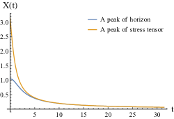
Figure 11: The peaks of the horizon and the energy-momentum tensor (we set $L=2\pi$). At late times, the location of one of the peak of the horizon coincides with the propagation of the holomorphic energy-momentum tensor. Another peak coincides with anti-holomorphic one. The peak of energy-momentum tensor at $t=0$ coincides with $X=L/2$.

5.2 The Möbius quench

The metric for the state quenched by the Möbius Hamiltonian is represented by $f_{tt,i=1,2},f_{xx,i=1,2}$ in Appendix C.1, and $f_{tx}$ is replaced by the one in Appendix C.2. Introduce a new radial coordinate $r^{\prime}=r\sqrt{-f_{xx,1}}$ similarly to the SSD case. The position of the horizon in $r^{\prime}$ coordinate is shown in Fig. 12. The time dependence of the position of this horizon has the periodicity $2\pi/\Omega=L\cosh{2\theta}$.

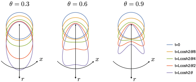
Figure 12: Time dependence of the position of the horizon.

The time when the horizon saddle appears at position $X$ is given by

$$t=\frac{L\cosh{2\theta}}{\pi}\tan^{-1}\frac{\sqrt{2\tanh 2\theta\cos\left(\frac{2\pi X}{L}\right)-1}}{\sqrt{\cosh 4\theta-\sinh 4\theta\cos\left(\frac{2\pi X}{L}\right)}},\,\quad t=mL\cosh{2\theta}$$ (5.8)

where $m$ are integers. This is given by solving the equation $\partial_{X}r^{\prime}_{\rm horizon}=0$ with respect to $t$. This approaches (5.4) in the SSD limit $\theta\rightarrow\infty$. By plugging this into $r^{\prime}_{\rm horizon}=r_{0}\sqrt{-f_{xx,1}}$, we obtain the $X$ dependence of the horizon at time (5.8),

$$r^{\prime}_{\text{horizon}}=\frac{2r_{0}\sinh 2\theta}{\sqrt{\cosh 4\theta-\cos\frac{2\pi X}{L}\sinh 4\theta}}.$$ (5.9)

The position of the peak at time $t$ is given by

$$X=\frac{L}{\pi}\tan^{-1}e^{-2\theta}\sqrt{\frac{(\sinh 4\theta-2)+(\cosh 4\theta-1)\cos\left(\Omega t\right)}{(\sinh 4\theta+2)-(\cosh 4\theta-1)\cos\left(\Omega t\right)}}\,.$$ (5.10)

This is given by solving the equation $\partial_{t}r^{\prime}_{\rm horizon}=0$ with respect to $X$. The time dependence of the radius of the horizon at $x=X$ is given by plugging this into $r^{\prime}_{\rm horizon}=r_{0}\sqrt{-f_{xx,1}}$ as

$$r^{\prime}_{\text{horizon}}=r_{0}\sqrt{\cosh^{2}2\theta\sec^{2}\left(t\Omega/2\right)-\sinh^{2}2\theta}\,.$$ (5.11)

5.3 Time evolution of bulk excitations in the SSD/Möbius quench

In the above, we studied the time-evolution of the black hole horizon in the SSD and Möbius quenches. As pointed out in Sec. 4, the thermal states are well approximated by the high-energy eigenstates. In this section, we especially consider the states created by inserting spinless primary operators ${\cal O}_{h}$ with conformal dimensions $h_{L}=h_{R}=h$ on the vacuum state. It is known that a primary operator ${\cal O}_{h}$ with large conformal dimension $h>\frac{c}{24}$ creates a black hole in AdS with temperature

$$T=\frac{1}{2\pi}\sqrt{\frac{24h}{c}-1}\,.$$ (5.12)

On the other hand, a primary operator ${\cal O}_{h,\bar{h}}$ with small conformal dimension $c\gg h$ creates a small bulk excitation on the pure AdS spacetime created by the matter fields dual to ${\cal O}_{h,\bar{h}}$. In this section, we consider how this small bulk excitation time-evolves under the SSD and Möbius quenches.

Let us insert a primary operator at the center of the Euclidean plane $z=\bar{z}=0$, i.e., $\tau=-\infty$ in the Euclidean time,

$$|\psi_{{\cal O}_{h}}\rangle={\cal O}_{h,\bar{h}}(z=0,\bar{z}=0)|0\rangle\,.$$ (5.13)

This is dual to a bulk excitation centered at the origin of the AdS spacetime. We are interested in how this excitation moves as it is time-evolved by the SSD or Möbius Hamiltonian. The dual CFT state we will consider is given by

$$|\psi_{{\cal O}_{h,\bar{h}}}(t)\rangle=e^{-iH_{\text{SSD }}t}{\cal O}_{h,\bar{h}}(z=0,\bar{z}=0)|0\rangle\,.$$ (5.14)

The strategy that we will use here is summarized in [107], where they move the bulk excitation by acting with the corresponding bulk $SL_{2}$ generators. We will explain the details below. Let us assume the primary operator is decomposed into products of chiral and anti-chiral parts

$${\cal O}_{h,\bar{h}}(z,\bar{z})=\sum_{i}{\cal O}_{h}^{i}(z){\cal O}_{\bar{h}}^{i}(\bar{z})\,,$$ (5.15)

which have dimensions $h\neq 0,\bar{h}=0$ and $h=0,\bar{h}\neq 0$ respectively. We first consider the chiral (spinning) state created only by ${\cal O}_{h}^{i}(z)$ instead of considering ${\cal O}_{h,\bar{h}}(z,\bar{z})$ itself;

$$|\psi_{{\cal O}_{L}}\rangle={\cal O}_{h}(z=0)|0\rangle\,,$$ (5.16)

where we omit the $i$-label for simplicity. It corresponds to a spinning BTZ black hole (or a small spinning excitation in the pure AdS) with mass $m=\sqrt{h(h-2)}$ and spin $s=h$.

The SSD Hamiltonian as the time-translation in the Poincaré coordinate

Before considering the evolution of the black hole or the bulk excitation generated by the SSD/Möbius Hamiltonian, we introduce new coordinates in which actions of these Hamiltonians are simple.

The evolution under the SSD Hamiltonian is simplified by introducing the boundary Poincaré coordinate $(z_{P},\bar{z}_{P})$. The boundary global coordinate $(w,\bar{w})$ and the boundary Poincaré coordinate $(z_{P},\bar{z}_{P})$ are related as

$$iz_{P}=L/\tan\left(\frac{i\pi w}{L}\right)\,,\quad i\bar{z}_{P}=L/\tan\left(\frac{i\pi\bar{w}}{L}\right)\,,$$ (5.17)

where $z_{P}=\tau_{P}+ix_{P}$ and $\bar{z}_{P}=\tau_{P}-ix_{P}$ are the complex coordinates in the Poincaré coordinate. The symbol $\tau_{P}$ is the Euclidean time coordinate, and $x_{P}$ is the spatial coordinate ($-\infty<x_{P}<\infty$) in the plane where the Poincaré coordinate is defined. Notice that in this Poincaré coordinate, the two fixed points of the SSD Hamiltonian is located at the origin and the spatial infinity.

Now let us see how the Poincaré coordinate simplifies the translation under the SSD Hamiltonian. The flow of the Poincaré time is generated by the following Hamiltonian

$$H_{P}=\int^{\infty}_{-\infty}dx_{P}T_{\tau_{P}\tau_{P}}(x_{P})=-i\int dz_{P}T(z_{P})-i\int d\bar{z}_{P}\overline{T}(\bar{z}_{P})\,.$$ (5.18)

We use the usual transformation rule for the energy-momentum tensor

$$\left(\frac{dz_{P}}{dw}\right)^{2}T\left(z_{P}\right) =T(w)-\frac{c}{24\pi}\mathrm{Sch}\left(z_{P},w\right)$$

$$=T(w)+\frac{\pi c}{12L^{2}}\,,$$ (5.19)

with $\frac{dz_{P}}{dw}=\frac{\pi}{L\sin^{2}\left(\frac{i\pi w}{L}\right)}$ and move to the original global coordinate $(w,\bar{w})$ as

$$H_{P} =\oint\frac{dw}{iL}\left(\frac{dw}{dz_{P}}\right)\left(T(w)+\frac{\pi c}{12L^{2}}\right)+\oint\frac{d\bar{w}}{iL}\left(\frac{d\bar{w}}{d\bar{z}_{P}}\right)\left(\overline{T}(\bar{w})+\frac{\pi c}{12L^{2}}\right)$$

$$=\int\frac{dx}{2\pi}2\sin^{2}\left(\frac{\pi x}{L}\right)T_{\tau\tau}(x)+\frac{c}{12L}$$

$$=H_{\rm SSD}+\frac{c}{12L}\,.$$ (5.20)

Therefore, the SSD Hamiltonian generates the time-flow in the Poincaré coordinate defined as (5.17). This indicates that a black hole (or the bulk excitation) dual to the state (5.14) moves along the Poincaré time direction. Static objects in the bulk Poincaré coordinate are seen as ones falling to the asymptotic boundary of the AdS over an infinitely long time from the perspective of the boundary observer in the global coordinate. Thus, we expect that the black hole (or the bulk excitation) after the SSD quench gets closer and closer to the AdS boundary as time evolves. We will justify this expectation by explicit computations in the following.

General Möbius case

The general Möbius Hamitonians can also be identified to the generators of time-directions in new coordinate systems $(z_{\theta},\bar{z}_{\theta})$. The relation to the original global coordinate is given by

$$\tan\frac{iz_{\theta}}{2L\cosh 2\theta}=e^{-2\theta}/\tan\left(\frac{i\pi w}{L}\right)\,,\quad\tan\frac{i\bar{z}_{\theta}}{2L\cosh 2\theta}=e^{-2\theta}/\tan\left(\frac{i\pi\bar{w}}{L}\right)\,.$$ (5.21)

This coordinate $(z_{\theta},\bar{z}_{\theta})$ approaches the Poincaré coordinate $(z_{P},\bar{z}_{P})$ (5.17) as we send $\theta\rightarrow\infty$. Let us check the Hamiltonian $H_{\theta}$ associated to this new coordinate $(z_{\theta},\bar{z}_{\theta})$ indeed gives the Möbius Hamitonian. The Hamiltonian $H_{\theta}$ is given by

$$H_{\theta}=-i\int dz_{\theta}T(z_{\theta})-i\int dz_{\theta}\overline{T}(\bar{z}_{\theta})\,.$$ (5.22)

Again, by using the transformation rule of the energy-momentum tensor

$$\left(\frac{dz_{\theta}}{dw}\right)^{2}T\left(z_{P}\right) =T(w)-\frac{c}{24\pi}\mathrm{Sch}\left(z_{\theta},w\right)$$

$$=T(w)+\frac{\pi c}{12L^{2}}-\frac{\pi c}{12L^{2}\cosh^{2}\theta}\frac{1}{(1-\tanh 2\theta\cos\left(\frac{2i\pi w}{L}\right))^{2}}\,,$$ (5.23)

with

$$\frac{dz_{\theta}}{dw}=\frac{2\pi}{1-\tanh 2\theta\cos\left(\frac{2\pi x}{L}\right)}\,,$$ (5.24)

we obtain

$$H_{\theta} =\int\frac{dx}{2\pi}\left(1-\tanh 2\theta\cos\left(\frac{2i\pi w}{L}\right)\right)T_{\tau\tau}(x)+\frac{c}{12L}\,$$

$$=H_{\text{M\"{o}bius}}+\frac{c}{12L}\,.$$ (5.25)

Therefore, the Möbius Hamiltonian generates the time-flow in the coordinate defined as (5.21).

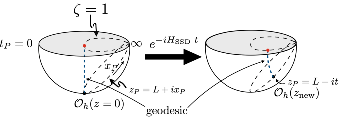
Figure 13: The gray disks correspond to the $t_{P}=0$ in the Poincaré coordinate (i.e., $t=0$ in the global coordinate) slices of the bulk AdS spacetime. The hemisphere attached to each disk represents the Hyperbolic disk corresponding to $-\infty<\tau<0$ ($|z|<1$) in the Euclidean AdS boundary. Left: Inserting a chiral primary operator ${\cal O}_{h}$ at the origin of the hyperbolic disk $z=0$ (i.e., $\tau=-\infty$) creates the bulk excitation around the center of the AdS, i.e., $\zeta=1,x_{P}=0$ on the $t_{P}=0$ slice in the bulk Poincaré coordinate. Right: The evolution under the SSD Hamiltonian $e^{-iH_{\rm SSD}t}$ moves the position of the primary operator along $z_{P}=L-it$ in the Poincaré coordinate. Correspondingly, the center of the bulk excitation also moves to $\zeta=1,x_{P}=-t$ on the $t_{P}=0$ slice. The map between the boundary and the bulk is simply represented by the geodesic connecting them.

Map between the boundary and the bulk

We now return to the time-evolution of the CFT state dual to the black hole or the bulk excitation. First, we simply consider how the chiral part is time-evolved by the SSD Hamiltonian

$$\left|\psi_{{\cal O}_{h}}^{\text{SSD }}(t)\right\rangle=e^{-iH_{\text{SSD }}t}{\cal O}_{h}(z=0)|0\rangle\,,$$ (5.26)

and see how the corresponding bulk excitation moves as time evolves. Let us insert a primary operator at the infinite past in the Euclidean global coordinate $w=-\infty$, i.e., $z=0$ in the plane coordinate given by the exponential map $z=e^{\frac{2\pi w}{L}}$ from $w$. This corresponds to inserting the operator at $z_{P}=L$ ($\tau_{P}=L$) in the Poincaré coordinate. This insertion of the primary operator creates a bulk excitation (or a black hole) centered at the origin of the AdS at $t=0$ time slice. This corresponds to $(\zeta,x_{P})=(1,0)$ at the same time slice in the bulk Poincaré coordinate, where $\zeta$ is the coordinate corresponding to the bulk direction.

The action of $e^{-iH_{\text{SSD }}t}$ moves the operator to the insertion point $z_{\rm new}$ on the Euclidean boundary. This creates the bulk excitation centered at the corresponding bulk point, which is away from the origin as depicted in Fig. 13. The bulk point is determined by the intersection between $t=0$ slice of the AdS and the geodesic in the Euclidean AdS starting from $z_{\rm new}$ as pointed out in [107].

Let us remind ourselves that the evolution generated by the SSD Hamiltonian gives the time-evolution in the boundary Poincaré coordinate. Therefore, the chiral primary operator ${\cal O}_{h}$ inserted at the origin of the $z$ coordinate (equivalently at $z_{P}=L$ in the Poincaré coordinate) moves as

$$e^{-iH_{\mathrm{SSD}}t}{\cal O}_{h}(z_{P}=L)e^{iH_{\mathrm{SSD}}t}={\cal O}_{h}(z_{P}=L-it).$$ (5.27)

Since $z_{P}=\tau+ix_{P}$, we can interpret it that in the Euclidean regime, the insertion point moves from $x_{P}=0$ to $x_{P}=-t$ on the $\tau_{P}=L$ slice. This is schematically drawn as Fig. 13. Correspondingly, the bulk excitation, which is originally centered at the origin of the AdS: $(\zeta,x_{P})=(1,0)$, moves to $(\zeta,x_{P})=(1,-t)$ by action of the SSD Hamiltonian as depicted in Fig. 14. Thus, the bulk excitation corresponding to the chiral part of the original primary operator approaches to the fixed point of the SSD quench, i.e., $x_{P}=\infty$ in the Poincaré coordinate, $x=0$ in the global coordinate while rotating in the negative direction of $x$ (and $x_{P}$).

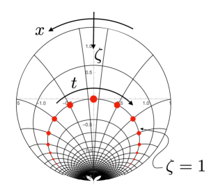
Figure 14: The bulk excitation corresponding to the time-evolved CFT chiral primary operator $e^{-iH_{\text{SSD}}t}{\cal O}_{h}(z=0)e^{iH_{\text{SSD}}t}$ drawn in the global AdS. The outermost circle corresponds to the boundary of the AdS, where $\zeta=0$ in the Poincaré coordinate. The point at the bottom of the circle corresponds to infinity in the Poicaré coordinate: $\zeta=\infty$. The distorted circles with $\zeta=\infty$ as a fixed point are the constant $\zeta$ slices. The curves orthogonal to them corresponds to the constant $x_{P}$ slices. The center of the bulk excitation at each time $t$ is depicted as a red point. It moves along the $\zeta=1$ slice as time evolves.

Similarly, the anti-chiral part of the original primary operator moves as

$$e^{-iH_{\mathrm{SSD}}t}{\cal O}_{\bar{h}}(\bar{z}_{P}=L)e^{iH_{\mathrm{SSD}}t}={\cal O}_{\bar{h}}(\bar{z}_{P}=L-it)\,,$$ (5.28)

thus the corresponding bulk excitation moves from $(\zeta,x_{P})=(1,0)$ to $(\zeta,x_{P})=(1,t)$. That is, it approaches the fixed point of the SSD quench while rotating in the direction of positive $x$ (and $x_{P}$). Since the original scalar primary operator ${\cal O}_{h,\bar{h}}$ is created by the products of the chiral and anti-chiral parts as (5.15), the bulk excitation corresponding to ${\cal O}_{h,\bar{h}}$ just approaches the fixed point along $x_{P}=0$ without rotation.

To see the profile of the time-evolved bulk excitation more explicitly, let us compute the overlap between the state

$$|\phi_{{\cal O}_{h,\bar{h}}}(\zeta,x_{P})\rangle=\phi_{{\cal O}_{h,\bar{h}}}(\zeta,x_{P})|0\rangle$$ (5.29)

excited by the bulk local operator $\phi_{{\cal O}_{h,\bar{h}}}(\zeta,x_{P})$ dual to the primary operator ${\cal O}_{h,\bar{h}}$ and the excited states evolved under the SSD Hamiltonian $|\psi_{{\cal O}_{h,\bar{h}}}^{\text{SSD }}(t)\rangle$ (5.14). Let us remind ourselves that when the primary operator is inserted at the origin $(\tau_{P}=0,x_{P}=0)$ in the boundary Poincaré coordinate, the overlap is just given by the usual bulk-to-boundary propagator

$$\left\langle\phi(\zeta,x_{P})|{\cal O}_{h,\bar{h}}\left(\tau_{P}=0,x_{P}=0\right)\right\rangle=\frac{\zeta^{2h}}{\left(\zeta^{2}+x_{P}^{2}\right)^{2h}}\,.$$ (5.30)

As explained above, the SSD quenched state $|\psi_{{\cal O}_{h,\bar{h}}}^{\text{SSD }}(t)\rangle$ can be obtained by inserting the primary operator at $z_{P}=L-it,\bar{z}_{P}=L-it$. In the Lorentzian regime obtained by the Lorentzian rotation $\tau_{P}\rightarrow\tau_{P}-it_{P}$, the complex coordinate becomes $z_{P}=\tau_{P}-i(t_{P}-x_{P}),\bar{z}_{P}=\tau_{P}-i(t_{P}+x_{P})$. Therefore, we can regard the operator as being inserted at a complex time $t_{p}=t+iL$ in the Poincaré coordinate. Thus, simple modifications to the bulk-to-boundary propagator above lead to

$$\langle\phi(\zeta,x_{P})|\psi_{{\cal O}_{h,\bar{h}}}^{\text{SSD }}(t)\rangle=\frac{\zeta^{2h}}{\left(\zeta^{2}+x_{P}^{2}-(t+iL)^{2}\right)^{2h}}\,,$$ (5.31)

for the overlap between the bulk locally excited state $|\phi_{{\cal O}_{h,\bar{h}}}(\zeta,x_{P})\rangle$ and the SSD quenched state $|\psi_{{\cal O}_{h,\bar{h}}}^{\text{SSD }}(t)\rangle$. We plot the contours orresponding to $|\langle\phi(\zeta,x_{P})|\psi_{{\cal O}_{h,\bar{h}}}^{\text{SSD }}(t)\rangle|=1$ for several values of $t$ in Fig. 15.

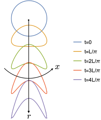
Figure 15: Contours corresponding to $|\langle\phi(r,x)|\psi_{{\cal O}_{h,\bar{h}}}^{\text{SSD }}(t)\rangle|=1$ for several values of $t$ depicted in the global coordinate. Here, we set $L=2\pi$ and $h=2$. By properly shifting the center of each excitation using the AdS isometry, the contours nicely match those for the black hole horizon Fig. 10 .

As we expected, the bulk excitation approaches the fixed point without rotation as time evolves. Moreover, by properly shifting the center of each excitation using the AdS isometry, the contours nicely match those for the black hole horizon Fig. 10.

6 Mutual information

The von Neumann entropy for single intervals (Sec. 3) and the energy density/current (Sec. 4) are found to be insensitive to the details of CFTs. However, the theory dependence should show up in more complex probes such as mutual information defined for two intervals and higher-point correlation functions. In this section, we consider mutual information for the free fermion CFT and holographic CFT. Two-point correlation functions are analyzed in Appendix D.

We first recall that for two subsystems $A$ and $B$, the mutual information $I_{A,B}$ is defined by a linear combination of entanglement entropy (von Neumann entropy):

$$I_{A,B}=S_{A}+S_{B}-S_{A\cup B}.$$ (6.1)

We note that the mutual information is free from the UV divergence when $A\cap B=0$, i.e., $I_{A,B}$ is finite even if the lattice spacing is $0$, while keeping $\epsilon$ (inverse temperature) finite. Our choices of the subsystems (subintervals) will be given below.

For both free fermion and holographic CFTs, we will find that the mutual information after the SSD quench, at late enough times, is essentially given by the mutual information of the uniform ground state (except in some special cases where one of the endpoints of the subsystems is on the fixed point): The difference between $I_{A,B}$ for our state $\rho(t)=e^{-itH_{\mathrm{SSD}}}\rho(0)e^{itH_{\mathrm{SSD}}}$ and the state in (1.7) is at most $\mathcal{O}(1)$. We will thus confirm that the density operator at late times can be approximated by (1.7). Namely, “reverse” thermalization occurs by the SSD quench where the correlations between subsystems of the initial thermal state undergo a crossover to those of the ground state without any non-unitary operations. We will also discuss a finer structure of the late time state beyond the approximation (1.7).

6.1 Holographic CFT

Case (a)

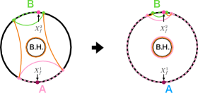
Case (b)

Figure 16: A sketch of the time evolution of the minimal surfaces for $S_{A}$ (pink solid), $S_{B}$ (green solid) and $S_{A\cup B}$ (orange solid) in the Heisenberg picture. The subsystem $A$ and $B$ are represented by pink dotted and green dotted lines, respectively.

Let us first discuss the time-evolution of the mutual information in holographic CFT after the SSD quench. We consider two cases and take the subsystems $A$ and $B$ as follows. In case (a), the fixed point $x=X^{1}_{f}$ is included neither in the subsystem $A$ nor in $B$ (Fig. 16(a)). On the other hand, in case (b), the fixed point $x=X^{1}_{f}$ is included in the subsystem $A$ but not in $B$ (Fig. 16(b)). In the Heisenberg picture, the twist and anti-twist operators defining the subsystems flow and, after enough time has passed, meet at the other fixed point $x=X^{2}_{f}$ (both in case (a) and (b) – see Fig. 16). As a result, the minimal surface for $S_{B}$ leaves the black hole, so $S_{B}$ becomes independent of temperature and can be approximated by the entanglement entropy of the ground state $S^{\text{vac}}_{B}$. In case (a), after enough time has passed, the minimal surfaces for $S_{A}$ and $S_{A\cup B}$ are far enough away from the black hole so that $S_{A}$ and $S_{A\cup B}$ can be approximated by the entanglement entropy of the ground state, $S^{\text{vac}}_{A}$ and $S^{\text{vac}}_{A\cup B}$, respectively. On the other hand, in case (b), at late times, the minimal surface for $S_{A}$ wraps around the black hole and the minimal surfaces for $S_{A\cup B}$ are located near the boundary of the AdS. Consequently, $S_{A}$ and $S_{A\cup B}$ are given by the thermal entropy $S_{\text{thermal}}$ and the entanglement entropy of the ground state, $S^{\text{vac}}_{A}$ and $S^{\text{vac}}_{A\cup B}$, respectively. To summarize, in both cases (1) and (2), after enough time has passed, $I_{A,B}$ is given by the mutual information $I^{\text{vac}}_{A,B}$ of the ground state, i.e.,

$$I_{A,B}\approx I^{\text{vac}}_{A,B}=\text{Max}\left[0,S^{\text{vac}}_{A}+S^{\text{vac}}_{B}-S^{\text{vac}}_{\text{Con.}}\right],$$ (6.2)

where $S^{\text{vac}}_{\text{Con.}}$ is the area of the minimal surface connecting the subsystems in the vacuum state.

6.2 The free fermion CFT

The mutual information for the case of free fermion CFT, for both SSD and Möbius quenches, can be computed explicitly (using the bosonization approach, that is also used in the computation of the von Neumann entropy). It can be expressed as a sum of the spin-structure independent and dependent terms as

$$I_{A\cup B,\nu\\ }^{(N)}=I_{A\cup B,\text{univ.}}^{(N)}+I_{A\cup B,\nu,\text{non-univ.}}^{(N)}$$ (6.3)

where

$$I_{A\cup B,\text{univ.}}^{(n)}= \frac{n+1}{12n}\log\left|\frac{\vartheta_{1}\left(\frac{w_{X_{2}}^{\text{new}}-w_{X_{4}}^{\text{new}}}{2\epsilon}|\tau\right)\vartheta_{1}\left(\frac{w_{X_{1}}^{\text{new}}-w_{X_{3}}^{\text{new}}}{2\epsilon}|\tau\right)}{\vartheta_{1}\left(\frac{w_{X_{2}}^{\text{new}}-w_{X_{3}}^{\text{new}}}{2\epsilon}|\tau\right)\vartheta_{1}\left(\frac{w_{X_{4}}^{\text{new}}-w_{X_{1}}^{\text{new}}}{2\epsilon}|\tau\right)}\right|^{2},$$ (6.4)

$$I_{A\cup B,\nu,\text{non-univ.}}^{(n)}= \frac{1}{1-n}\sum_{k=-\frac{n-1}{2}}^{\frac{n-1}{2}}\log\left|\frac{\vartheta_{\nu}\left(\frac{k}{n}\frac{w_{X_{1}}^{\text{new}}-w_{X_{2}}^{\text{new}}}{2\epsilon}\bigg{|}\tau\right)\vartheta_{\nu}\left(\frac{k}{n}\frac{w_{X_{3}}^{\text{new}}-w_{X_{4}}^{\text{new}}}{2\epsilon}\bigg{|}\tau\right)}{\vartheta_{\nu}(0|\tau)\vartheta_{\nu}\left(\frac{k}{n}\frac{w_{X_{1}}^{\text{new}}-w_{X_{2}}^{\text{new}}+w_{X_{3}}^{\text{new}}-w_{X_{4}}^{\text{new}}}{2\epsilon}\bigg{|}\tau\right)}\right|^{2}$$

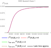
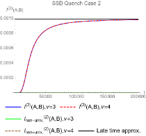
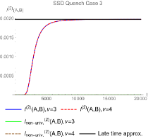
Figure 17: The second Rényi mutual information of the thermal state after the SSD quench for the three cases listed in (6.5) with $L=1000$, $X=10$ and $\epsilon=1$ for the two physical spin structures $\nu=3,4$. The blue and red curves correspond to the total mutual information (6.3) while the green and brown curves correspond to the non-universal spin-structure term in (6.4). The black line is the late time approximation to the second Rényi mutual information (6.2).

In Fig. 17, the mutual information after the SSD quench is plotted for the following three choices of the subsystems:

$$\begin{split}&A=\left\{x\big{|}0\leq x\leq X,L-X\leq x\leq L\right\},~{}~{}B=\begin{cases}\left\{x\big{|}\frac{L}{4}-X\leq x\leq\frac{L}{4}+X\right\}&~{}\text{Case~{}1}\\ \left\{x\big{|}\frac{L}{2}-X\leq x\leq\frac{L}{2}+X\right\}&~{}\text{Case~{}2}\\ \end{cases},\\ &A=\left\{x\bigg{|}\frac{L}{4}-X\leq x\leq\frac{L}{4}+X,\right\},~{}~{}B=\left\{x\bigg{|}\frac{L}{2}-X\leq x\leq\frac{L}{2}+X\right\}~{}\text{Case~{}3},\end{split}$$ (6.5)

for the physical spin structures $\nu=3,4$ which are identical. In all these cases with $\epsilon$ much smaller than the other length scales, the non-universal piece is essentially zero. In the following, we will focus on the universal spin structure independent term in (6.4). In all three cases, the mutual information simply grows and saturates at a late time value that we will discuss momentarily. The most salient features of these plots are the saturation values of the mutual information as well as the time it takes for the saturation to occur. The saturation values for cases 1 and 3 are identical and greater than the saturation value in case 2. As we will see momentarily, this is because the separation between the pair of intervals is the same for cases 1 and 3 which is smaller than the separation between the pair of intervals in case 2. The mutual information saturates much faster in case 3 than in cases 1 and 2, and marginally faster in case 2 than in case 1. This is likely due to the fact that the pair of intervals in case 3 is situated away from the SSD fixed point $x=X^{1}_{f}$ while one of the intervals in cases 1 and 2 contains this fixed point where the envelope function of the SSD Hamiltonian vanishes. Saturation of the mutual information is achieved in case 2 slightly earlier than in case 1 likely due to the smaller separation between the two intervals.

The late time saturation value can be studied analytically. At late time $t\gg L\gg\epsilon$, the universal part of the mutual information (6.4) is approximately given by

$$\lim_{t\rightarrow\infty}I_{A\cup B,\text{univ.}}^{(n)} =\frac{n+1}{6n}\log\left|\frac{\left(\tan\frac{\pi X_{1}}{L}-\tan\frac{\pi X_{3}}{L}\right)\left(\tan\frac{\pi X_{2}}{L}-\tan\frac{\pi X_{4}}{L}\right)}{\left(\tan\frac{\pi X_{1}}{L}-\tan\frac{\pi X_{4}}{L}\right)\left(\tan\frac{\pi X_{2}}{L}-\tan\frac{\pi X_{3}}{L}\right)}\right|$$

$$=\frac{n+1}{6n}\log\left|\frac{\sin{\frac{\pi(d+L_{1})}{L}}\sin{\frac{\pi(d+L_{2})}{L}}}{\sin{\frac{\pi d}{L}}\sin{\frac{\pi(d+L_{1}+L_{2})}{L}}}\right|$$ (6.6)

for all three cases 1, 2 and 3. In the second line, we introduce the lengths of the two subsystems, $L_{1}=X_{1}-X_{2}$ and $L_{2}=X_{3}-X_{4}$, and the separation $d=X_{2}-X_{3}$. This late time saturation value of the mutual information (6.2) is precisely the mutual information of the vacuum state [89, 92, 108, 109]. Furthermore, in the limit of well-separated small intervals, i.e., $L_{1},L_{2}\ll d$ where the separation $d$ is on the same order as the total system size $L$,

$$\frac{\sin{\frac{\pi(d+L_{1})}{L}}\sin{\frac{\pi(d+L_{2})}{L}}}{\sin{\frac{\pi d}{L}}\sin{\frac{\pi(d+L_{1}+L_{2})}{L}}}\approx 1+\frac{\pi^{2}L_{1}L_{2}}{L^{2}\sin^{2}\frac{\pi d}{L}}-\frac{\pi^{3}L_{1}L_{2}(L_{1}+L_{2})}{L^{3}\sin^{2}\frac{\pi d}{L}\tan\frac{\pi d}{L}}+\cdots$$ (6.8)

This approximation breaks down if $d\approx 0,L$ because of the tangent in the denominator of the third term in the series expansion of $\frac{L_{i}}{L}$. While the series expansion is valid, the late time saturation value of the mutual information (6.2) is approximately

$$\lim_{t\rightarrow\infty}I_{A\cup B,\text{univ.}}^{(n)}\approx\frac{n+1}{6n}\frac{\pi^{2}L_{1}L_{2}}{L^{2}\sin^{2}\frac{\pi d}{L}}.$$ (6.9)

Thus, the late time value of the mutual information decreases as a function of distance, which explains why the saturation value was smaller in case 2 than in cases 1 and 3, and why the saturation values appeared to be equal in cases 1 and 3 despite the intervals being located at different parts of the system.

Case 1

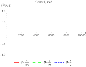
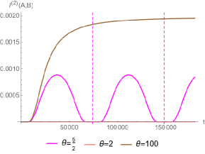
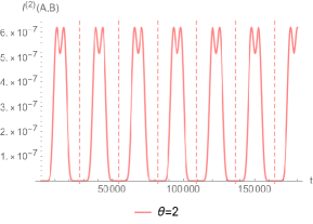
Case 2

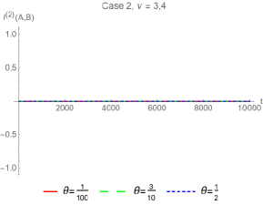
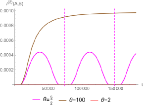
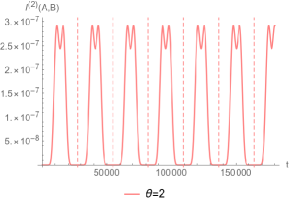
Case 3

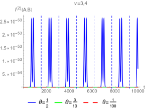
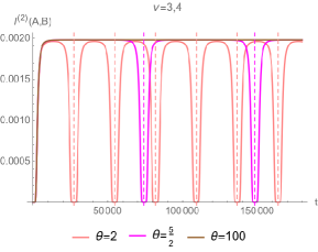
Figure 18: Plots of the second Rényi mutual information of the thermal state after a Möbius quench for the three cases listed in (6.5) with $L=1000$, $X=10$ and $\epsilon=1$ for the two physical spin structures $\nu=3,4$ which turn out to be identical. The dotted vertical lines indicate the periods $L\cosh{2\theta}$.

Moving away from the SSD limit, plots of the mutual information (6.3) after a general Möbius quench with finite deformation parameter $\theta$ are shown in Fig. 18. Just as in the SSD quench, the spin structure terms are negligible and the mutual information is the same for both $\nu=3$ and $\nu=4$. When $\theta$ is small, the deformed Hamiltonian is almost the uniform one, so the quench does nothing to the thermal state. Thus, the mutual information vanishes for small values of the deformation parameter $\theta$. As $\theta$ is increased, the mutual information starts to become non-zero and bumps with two peaks can be observed (c.f. $\theta=2$ for cases 1 and 2 and $\theta=\frac{1}{2}$ for case 3). As $\theta$ is increased further, the amplitude of the mutual information grows. Eventually, the bumps in the mutual information show only a single peak. In all cases, the period of oscillation is given by $L\cosh{2\theta}$. As $\theta$ becomes larger, the period keeps growing until the mutual information approaches that of the SSD quench as in Fig. 17. Therefore, the mutual information in the SSD quench can be thought of as the limit of the Möbius quench with an infinite period.

Comparing the various cases also yield interesting insights into the dynamics of the Möbius quench. Since the SSD quench is a limit of the Möbius quench, the mutual information after the Möbius quench is upper bounded by the late time saturation value of the mutual information after the SSD quench (6.2) which is a decreasing function of the separation between the two intervals. This explains why the mutual information in cases 1 and 3 are larger than the mutual information in case 2. However, the mutual information in case 3 is also larger than that in case 1. For instance, the mutual information when $\theta=\frac{1}{2}$ is non-negligible only in case 3 and the mutual information for $\theta=2,\frac{5}{2}$ only attains the upper bound in case 3. Furthermore, the mutual information grows much faster in case $3$ than in case $1$. This assortment of observations can likely be attributed to the fact that in case $3$, both intervals are located away from the SSD fixed point while one of the intervals contains the SSD fixed point in case 1.

6.3 Finer structure of the late time density matrix

We have so far established the approximation to the late time density matrix (1.7) to leading order, using von-Neumann entropy for a single interval, and also mutual information. A closer look at our mutual information calculation also reveals the deviation from (1.7) at subleading order. Specifically, we found the mutual information between a subsystem including the fixed point and another subsystem that does not include the fixed point can be non-zero at subleading order. We recall that in mutual information leading order contributions in $S_{A}$, $S_{B}$, $S_{A\cup B}$ cancel with each other. Hence, the subleading (sub-extensive) terms in the von Neumann entropy contribute to mutual information. (While the non-zero subleading contribution always occurs for the free fermion case, for the case of holographic CFT, it depends on the choice of the subsystems.) Thus, beyond leading order, the late time density matrix deviates from (1.7).

The above consideration also shows that our state acquires (quantum) correlations by the SSD evolution. At high enough temperatures, the initial state $\rho(0)$ has very little quantum correlations, $\rho_{A\cup B}\approx\rho_{A}\otimes\rho_{B}$, while at late enough times, the non-zero mutual information suggests that $\rho_{A\cup B}\neq\rho_{A}\otimes\rho_{B}$, i.e., a separable reduced density matrix can become entangled.

7 Discussion and outlook

We have studied inhomogeneous quantum quench using the Möbius and SSD Hamiltonians in (1+1)d CFT. In the SSD quench, at late enough times, a black-hole-like excitation emerges at the fixed point with as much information as the total thermal entropy, i.e., the density operator can be approximated by (1.7). In this section, we will further discuss our findings in the Möbius/SSD quench.

Experimental realizations in quantum simulators

Firstly, our setup can be adopted in recent experimental platforms, synthetic or designer quantum systems, such as ultracold atoms, Rydberg atoms, trapped ions, superconducting qubits, etc. These systems have been used as quantum simulators to study many-body quantum systems. For example, the Ising CFT critical point has been realized recently in a one-dimensional chain of Rydberg atoms created by optical tweezers [7, 110, 111]. The flexibility of the systems would allow us to create inhomogeneous quantum many-body Hamiltonians with the Möbius or SSD deformation. Many of our findings can then be directly tested in experiments in principle. In particular, the formation (and destruction) of a black-hole-like excitation, which has much resemblance with the formation and evaporation of a black hole as we will explain below can be simulated in the lab.

Measurement-induced transition

In Sec. 3, we found the crossover from the volume- to area-law entanglement for the subsystem not including the fixed point $x=X^{1}_{f}$. This reminds us of the measurements-induced transition in monitored quantum circuits [112, 113, 114, 115, 116]. Instead of introducing measurements, in our setup, we control the amount of dissipation by acting with the unitary $e^{-itH_{\mathrm{SSD}}}$. In the holographic dual language, the unitary deforms the horizon of the BTZ black hole and controls locally the distance between the horizon and the boundary (the origin). We also note that in the volume-law phase of the monitored quantum circuits there is a sub-extensive term (logarithmic term) in the entanglement entropy that reflects non-trivial quantum error-correcting properties [117, 118, 119, 120]. As discussed in Sec. 6.3, we note that our late time state after the SSD quench also exhibits a finer structure – in addition to the leading contribution of the von-Neumann entropy indicating the formation of a black-hole-like excitation, there are subleading, logarithmic contributions that contribute to the saturation value of mutual information and indicate the deviation from (1.7). Investigating further the properties of the fine structure, and its possible connection to quantum-error-correcting properties, is an interesting future direction.

Simulation of formation and evaporation of a black hole

The SSD quench process, which collects the degrees of freedom to create a black-hole-like excitation at the origin, can be thought of as a process of creating a black hole. In the holographic picture, near the origin, the bulk horizon asymptotically approaches the boundary, and hence the black hole “expands” from the point of view of a local subregion near the origin. (Contrary, for subsystems not including the origin, the black hole “shrinks”.) We can also consider the time-reversal of these processes, i.e., $e^{+itH_{\mathrm{SSD}}}$ instead of $e^{-itH_{\mathrm{SSD}}}$, where the black hole shrinks near the origin and expands for regions away from the origin. Thus, our SSD quench can be used to test/simulate the formation and evaporation of a black hole in the experimental systems mentioned above (Fig. 6). In this interpretation, the von-Neumann entropy of a subsystem including the fixed point $x=X^{1}_{f}$ (subsystem $B$ in Fig. 6(b)), at late times, is interpreted as the entanglement entropy between late-time radiation and the black hole. On the other hand, for a subsystem not including the fixed point $x=X^{1}_{f}$ the von-Neumann entropy (at late times) is interpreted as the entanglement entropy of early-time radiations.

We note that the evolution by the SSD/Möbius Hamiltonian itself gives rise to Killing horizons: Choosing these generators as the time-evolution operator corresponds to choosing a particular Killing vector, which may result in the presence of a Killing horizon [121]. In the SSD limit, we have an extremal Killing horizon. Killing horizons may also emerge effectively by periodically driving the system using these generators, i.e., at the level of Floquet Hamiltonians [64, 65]. Based on this observation, in [64, 65], it was proposed that the optical lattice system can be used to simulate how excitations propagate in the space-time where a black hole exists. In contrast, in this work, a non-equilibrium process in which a black hole itself emerges or evaporates can be simulated by exciting a thermal equilibrium state with an inhomogeneous quench. In the holographic picture, we have a bulk black hole horizon (in contrast to the Killing horizons) since our initial state is a thermal state.

Creation of a low-entropy (low-temperature) state by local measurements

From a slightly practical point of view, our SSD quench protocol can be used to heat/cool a particular local region of the system. Furthermore, for $t\gg t_{*}$, once a black-hole-like excitation is created at the origin, it may be interesting to “remove” the black-hole-like excitation to cool the entire system. This may be achieved by turning off the coupling between the origin and the rest of the system. It is also interesting to perform a projective measurement at the origin: If we perform the projective measurement [122] by the state of $\left|\Psi\right>_{A}$ in subsystem $A$, the state transitions from (1.7) to

$$\rho\rightarrow\rho^{\prime}=\left|\Psi\right>_{A}\left<\Psi\right|_{A}\otimes\mathrm{Tr}_{A}\left|0\right>\left<0\right|.$$ (7.1)

The entropy after this measurement is given by

$$S_{\text{thermal}}\approx S_{A}=\frac{c}{3}\log{\left[\frac{\pi}{L}\sin{\left(\frac{\pi l}{L}\right)}\right]},$$ (7.2)

which is at most a quantity of $\mathcal{O}(1)$ ($l$ is the size of subsystem $A$). In this way, the SSD time evolution combined with a local projection measurement induces a transition from a high-entropy (high-temperature) to low-entropy (low-temperature) state.

This transition can be also discussed in the gravity dual in the Schrödinger picture (Fig. 19). At $t=0$, there is a spherically symmetric black hole with its center at the origin of ${\it AdS}$ spacetime. The SSD time-evolution deforms its shape for $t>0$. After enough time has passed, $t\gg t_{*}$, the black hole is deformed into a black brane-like shape extending from the origin of ${\it AdS}$ spacetime to its boundary near $x=X^{1}_{f}$. As a result, the black hole will be included in the bulk region that is dual to the subsystem $A$ containing the fixed point $x=X^{1}_{f}$, i.e., the entanglement wedge of $A$ [123, 124, 125, 126]. After this, the black hole can be removed by projective measurements in the subsystem $A$, and the measurement-induced phase transition from the BTZ black hole to the “almost” thermal ${\it AdS}_{3}$ can occur.

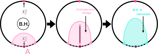
Figure 19: The time-evolution of a black hole after the SSD quench (left and middle) and subsequent projective measurement (right) in the Schrödinger picture. (Time flows from the left to right.) In the right image the black hole in the entanglement wedge is removed by the projective measurement.

It may also be possible to transfer energy between the system (the system quenched by the SSD evolution) and the observer performing the projective measurement. The energy for the total composite system (including both the CFT and the observer) should be conserved immediately before and after the measurement. The difference between the energy just before and after the measurement $\Delta E\approx\int_{A}dx\mathrm{Tr}\left(T_{00}(x)\rho_{\text{B.H.}}\right)-\int_{A}dx\left<\Psi\right|_{A}T_{00}(x)\left|\Psi\right>_{A}$ is the energy “extracted” by the measurement. The observer can thus obtain a large amount of energy of $\mathcal{O}\left({1}/{\epsilon}\right)$.

Outlook

As we demonstrated, by controlling the inhomogeneity of the system during dynamics, a rich variety of non-equilibrium many-body quantum states can be realized. Many of our findings can be directly tested by recent experimental platforms for quantum simulators. In particular, we proposed that the formation and evaporation processes of a black holes can be simulated in the SSD quench. The SSD quench can also be used as a method to create a low-temperature state. Finally, we close by listing some future directions.

First of all, our study in this paper is limited to (1+1)d CFT. It would be interesting to study inhomogeneous quenches in a wider class of systems, i.e., those that are not described by (1+1)D CFT, such as lattice spin systems away from critical points. In particular, we studied holographic CFTs as one of our examples, that exhibit strong quantum information scrambling [71, 72, 73, 74, 75, 76, 77, 78, 79, 80, 81, 82, 83]. It would be interesting to study other (non-CFT) systems that also exhibit quantum information scrambling, such as the chaotic quantum spin chain [127]. In this context, we can study the effects of the inhomogeneous dynamics on various “indicators” of quantum information scrambling, such as the level statistics, the spectral form factor, out-of-time-order correlators. It would be also interesting to study other types of dynamics, e.g., those that break ergodicity, such as many-body localizing dynamics [3, 4, 5, 6], and those that exhibit quantum many-body scars [7, 8, 9, 10, 11, 12, 13, 14].

Even within (1+1)D CFT, we can distinguish various kinds of dynamics, ranging from fully integrable (rational CFTs) to strongly “chaotic” (irrational/pure/holographic CFTs). In this paper, we took the free fermion CFT and holographic CFTs as representatives for each class. However, at the level of the von-Neumann entropy for a single-interval or one-point functions, their dynamics are rather indistinguishable. To distinguish the different types of dynamics, we need to study more sophisticated probes, such as the von-Neumann entropy for two or more subsystems (mutual information) and $n(\geq 4)$ point correlation functions. While we initiated the study of the mutual information in Sec. 6, the effects of inhomogeneity on dynamics (e.g., quantum information scrambling) needs to be studied in more detail.

Integrable and chaotic dynamics are described by different effective descriptions, the quasiparticle and membrane (line-tension) pictures [128, 129, 130, 131]. It is interesting to study how one can use these effective descriptions in the presence of inhomogeneity. In the current work, we are able to describe many (but not all) dynamical behaviors using the quasiparticle picture. The time evolution of von Neumann entropy for a subsystem not including a fixed point $x=X^{1}_{f}$ cannot be described by the quasiparticle picture for late times. It is thus interesting to construct an effective theory that can describe this regime where the quasiparticle picture is invalid. It is also interesting to understand the mechanism by which the quasiparticle picture breaks down.

Second, it would be interesting to study a wider class of inhomogeneous time-evolution operators. For example, [63] studied the dynamics of inhomogeneous Hamiltonians with an arbitrary smooth envelope function that can have more than one fixed points. Adapted to our setup, we expect that such dynamics can create multi black-hole-like excitations. This may allow us to construct the experimental systems that can simulate the process of two (more than one) merging black holes, and one black hole splitting into several black holes. Also, by engineering inhomogeneity, we may be able to create different kinds of non-equilibrium steady states, for example, those that support a steady thermal gradient. Another possible extension of the current work is to consider Floquet dynamics (and find its gravitational dual).

Appendix A Details of $\varphi$ and $\bar{\varphi}$

The variables $\varphi$ and $\bar{\varphi}$ for the Möbius time evolution operator are defined as

$$\begin{split}&\cos{\varphi}=r^{-1}\left[{\cos{\left({\pi X}/{L}\right)}\cos(\Omega t/2)-e^{2\theta}\sin{\left({\pi X}/{L}\right)}\sin(\Omega t/2)}\right],\\ &\sin{\varphi}=r^{-1}\left[{\sin{\left({\pi X}/{L}\right)}\cos(\Omega t/2)+e^{-2\theta}\cos{\left({\pi X}/{L}\right)}\sin(\Omega t/2)}\right],\\ &\cos{\bar{\varphi}}=\bar{r}^{-1}\left[{\cos{\left({\pi X}/{L}\right)}\cos(\Omega t/2)+e^{2\theta}\sin{\left({\pi X}/{L}\right)}\sin(\Omega t/2)}\right],\\ &\sin{\bar{\varphi}}=\bar{r}^{-1}\left[{-\sin{\left({\pi X}/{L}\right)}\cos(\Omega t/2)+e^{-2\theta}\cos{\left({\pi X}/{L}\right)}\sin(\Omega t/2)}\right],\\ &r=\bigg{[}\left(\cos{\left({\pi X}/{L}\right)}\cos(\Omega t/2)-e^{2\theta}\sin{\left({\pi X}/{L}\right)}\sin(\Omega t/2)\right)^{2}\\ &~{}~{}~{}~{}~{}+\left(\sin{\left({\pi X}/{L}\right)}\cos(\Omega t/2)+e^{-2\theta}\cos{\left({\pi X}/{L}\right)}\sin(\Omega t/2)\right)^{2}\bigg{]}^{\frac{1}{2}},\\ &\overline{r}=\bigg{[}\left(\cos{\left({\pi X}/{L}\right)}\cos(\Omega t/2)+e^{2\theta}\sin{\left({\pi X}/{L}\right)}\sin(\Omega t/2)\right)^{2}\\ &~{}~{}~{}~{}~{}+\left(-\sin{\left({\pi X}/{L}\right)}\cos(\Omega t/2)+e^{-2\theta}\cos{\left({\pi X}/{L}\right)}\sin(\Omega t/2)\right)^{2}\bigg{]}^{\frac{1}{2}}.\end{split}$$ (A.1)

In the SSD limit, $\varphi$ and $\bar{\varphi}$ (c.f. (2.12)) are defined as

$$\begin{split}&\cos{\varphi}=-\frac{\frac{2\pi t}{L}\sin{\left(\frac{\pi X}{L}\right)}-\cos{\left(\frac{\pi X}{L}\right)}}{r},\quad\sin{\varphi}=\frac{{\color[rgb]{0,0,1}+}\sin{\left(\frac{\pi X}{L}\right)}}{r},~{}~{}-\pi\leq{-\varphi}\leq 0,\\ &\cos{\bar{\varphi}}=\frac{\frac{2\pi t}{L}\sin{\left(\frac{\pi X}{L}\right)}+\cos{\left(\frac{\pi X}{L}\right)}}{\bar{r}},\ \quad\sin{\bar{\varphi}}=\frac{-\sin{\left(\frac{\pi X}{L}\right)}}{\bar{r}},~{}~{}-\pi\leq\bar{\varphi}\leq 0,\\ &r=\frac{1}{L}\sqrt{4\pi^{2}t^{2}\sin^{2}{\left(\frac{\pi X}{L}\right)}-4\pi tL\sin{\left(\frac{\pi X}{L}\right)}\cos{\left(\frac{\pi X}{L}\right)}+L^{2}},\\ &\bar{r}=\frac{1}{L}\sqrt{4\pi^{2}t^{2}\sin^{2}{\left(\frac{\pi X}{L}\right)}+4\pi tL\sin{\left(\frac{\pi X}{L}\right)}\cos{\left(\frac{\pi X}{L}\right)}+L^{2}}.\end{split}$$

Appendix B Time evolution of von Neumann entropy for the asymmetric subsystem.

In this section, we study the time evolution of the von Neumann entropy when the subsystem $A$ contains $X^{1}_{f}$ but $X^{1}_{f}$ is not the center of $A$. Here, the leftmost position of the subsystem is $Y$ and the rightmost position is $X$. We show the time evolution of the von Neumann entropy in this case in Fig. 20. The time evolution of von Neumann entropy in this case follows the quasiparticle picture in section 3.4.

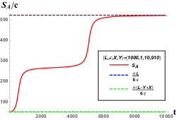
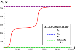
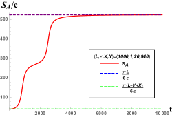
Figure 20: The time evolution of von Neumann entropy. The subsystem $A$ contains $X^{1}_{f}$, but $X^{1}_{f}$ is not at its center.

Appendix C Metric in the Schrödinger picture

Here we summarize the details of the metric in the Schrödinger picture.

C.1 Metric for the SSD quench

The metric components in (5.1) for the geometry dual to the state quenched by the SSD Hamiltonian are given by

$$\begin{split}&g(x,t)=16\pi^{2}L^{2}t^{2}\sin^{4}\left(\frac{\pi x}{L}\right)+\left(L^{2}-4\pi^{2}t^{2}\sin^{2}\left(\frac{\pi x}{L}\right)\right)^{2},\\ &f_{tt,1}=\frac{4L^{4}\sin^{4}\left(\frac{\pi x}{L}\right)}{g(x,t)},\quad f_{tt,2}=\frac{16L^{4}\sin^{4}\left(\frac{\pi x}{L}\right)\left(L^{2}+4\pi^{2}t^{2}\sin^{2}\left(\frac{\pi x}{L}\right)\right)^{2}}{g(x,t)^{2}},\\ &f_{xx,1}=-\frac{L^{4}}{g(x,t)},\quad f_{xx,2}=\frac{16\pi^{2}L^{6}t^{2}\sin^{2}\left(\frac{2\pi x}{L}\right)}{g(x,t)^{2}},\\ &\frac{f_{xx,2}}{f_{xx,1}}=-\frac{16\pi^{2}L^{2}t^{2}\sin^{2}\left(\frac{2\pi x}{L}\right)}{g(x,t)},\quad\frac{f_{tt,2}}{f_{tt,1}}=\frac{4\left(L^{2}-2\pi^{2}t^{2}\cos\left(\frac{2\pi t}{L}\right)+2\pi^{2}t^{2}\right)^{2}}{g(x,t)}.\\ &f_{tx}=\frac{16\pi L^{5}t\sin^{3}\left(\frac{\pi x}{L}\right)\cos\left(\frac{\pi x}{L}\right)\left(L^{2}-2\pi^{2}t^{2}\cos\left(\frac{2\pi x}{L}\right)+2\pi^{2}t^{2}\right)}{g(x,t)^{2}},\end{split}$$ (C.1)

These components satisfy

$$\frac{f_{tt,2}}{f_{tt,1}}+\frac{f_{xx,2}}{f_{xx,1}}=1.$$ (C.2)

The metric at $t=0$ is

$$ds^{2}=L^{2}\left[\frac{dr^{2}}{r^{2}-r_{0}^{2}}+\left[-\left(2\sin^{2}{\left(\frac{\pi x}{L}\right)}\right)^{2}(r^{2}-r_{0}^{2})dt^{2}+r^{2}dx^{2}\right]\right]\,,$$ (C.3)

which is obtained from a simple rescaling of the standard metric, $g_{tt}\rightarrow\left(2\sin^{2}{\left(\frac{\pi x}{L}\right)}\right)^{2}\cdot g_{tt}$. We also note that the metric at a fixed point $x=X^{1}_{f}$ is given by

$$ds^{2}=L^{2}\left[\frac{dr^{2}}{r^{2}-r_{0}^{2}}+r^{2}dx^{2}\right]\,,$$ (C.4)

and the metric at the other fixed point $x=X^{2}_{f}$ is

$$ds^{2}=L^{2}\left[\frac{dr^{2}}{r^{2}}+r^{2}\left(-f_{xx,1}dx^{2}-f_{tt,1}dt^{2}\right)\right]\,,$$ (C.5)

and $g_{rr}$ gets smaller in time, and it scales as $t^{-4}$ at late times. Near the boundary of the AdS $r=\frac{1}{a}\gg 1$, the geometry approaches

$$ds^{2} \approx L^{2}\left[\frac{dr^{2}}{r^{2}}-f_{tt,1}r^{2}dt^{2}-f_{xx,1}r^{2}dx^{2}\right]$$

$$=L^{2}\left[\frac{dr^{2}}{r^{2}}+r^{2}\frac{L^{4}dx^{2}-4L^{4}\sin^{4}{\left(\frac{\pi x}{L}\right)}dt^{2}}{16\pi^{2}L^{2}t^{2}\sin^{4}\left(\frac{\pi x}{L}\right)+\left(L^{2}-4\pi^{2}t^{2}\sin^{2}\left(\frac{\pi x}{L}\right)\right)^{2}}\right]\,$$ (C.6)

where $a$ is a lattice spacing.

C.2 Metric for the Möbius quench

The metric components for the geometry dual to the state quenched by the Möbius Hamiltonian are given by

$$\begin{split}&f_{tt,1}=\frac{\text{sech}^{2}(2\theta)\left(\tanh(2\theta)\cos\left(\frac{2\pi x}{L}\right)-1\right)^{2}}{D_{tt,1}},\quad f_{xx,1}=-\frac{1}{D_{xx,1}},\\ &f_{tt,2}=\frac{N_{tt,1}}{D_{tt,2}},\quad f_{xx,2}=\frac{4\sinh^{2}(2\theta)\sin^{2}\left(\frac{2\pi x}{L}\right)\sin^{2}\left(\Omega t\right)}{D_{xx,2}},\quad f_{tx,2}=\frac{N_{tx,1}}{D_{tx,2}},\\ \end{split}$$ (C.7)

where

$$\begin{split}&\textstyle A=\cosh^{2}(2\theta)-\sinh^{2}(2\theta)\cos\left(\Omega t\right)+\sinh(2\theta)\sin\left(\frac{2\pi x}{L}\right)\sin\left(\Omega t\right)-\sinh(4\theta)\cos\left(\frac{2\pi x}{L}\right)\sin^{2}\left(\Omega t\right),\\ &\textstyle B=-\cosh^{2}(2\theta)+\sinh^{2}(2\theta)\cos\left(\Omega t\right)+\sinh(2\theta)\sin\left(\frac{2\pi x}{L}\right)\sin\left(\Omega t\right)+\sinh(4\theta)\cos\left(\frac{2\pi x}{L}\right)\sin^{2}\left(\Omega t\right),\\ &D_{tt,2}=16AB^{2},\qquad D_{xx,2}=AB^{2},\qquad D_{t,x}=2A^{2}B^{2},\\ &\textstyle D_{tt,1}=\text{sech}^{2}(2\theta)\left[\cos^{2}\left(\frac{\Omega t}{2}\right)+\sin^{2}\left(\frac{\Omega t}{2}\right)\left(\cosh(4\theta)-\sinh(4\theta)\cos\left(\frac{2\pi x}{L}\right)\right)\right]^{2}\\ &\textstyle\qquad\qquad-\tanh^{2}(2\theta)\sin^{2}\left(\frac{2\pi x}{L}\right)\sin^{2}\left(\Omega t\right),\\ &\textstyle D_{xx,1}=A\left[\cosh^{2}(2\theta)-\sinh(4\theta)\cos\left(\frac{2\pi x}{L}\right)\sin^{2}\left(\frac{\Omega t}{2}\right)\right.\\ &\textstyle\left.\qquad\qquad\qquad-\sinh(2\theta)\left(\sinh(2\theta)\cos\left(\Omega t\right)+\sin\left(\frac{2\pi x}{L}\right)\sin\left(\Omega t\right)\right)\right],\\ &\textstyle N_{tt,1}=\left[6\cosh(4\theta)+6\cos\left(\Omega t\right)-6\cosh(4\theta)\cos\left(\Omega t\right)\right.\\ &\textstyle\qquad\qquad-8\cos\left(\frac{2\pi x}{L}\right)\left(\sinh{4\theta}-2\sinh(\theta)\cosh(\theta)\cosh(4\theta)\text{sech}(2\theta)\cos\left(\Omega t\right)\right)\\ &\textstyle\qquad\qquad\left.+8\sinh^{2}(2\theta)\cos\left(\frac{4\pi x}{L}\right)\sin^{2}\left(\frac{\Omega t}{2}\right)+2\right]^{2},\\ &\textstyle N_{tx}=\sinh(2\theta)\sin\left(\frac{2\pi x}{L}\right)\left[8\sin\left(\Omega t\right)\left(\cosh(2\theta)-\sinh(2\theta)\cos\left(\frac{2\pi x}{L}\right)\right)^{2}\right.\\ &\textstyle\qquad\qquad\left.+\tanh(2\theta)\sin\left(2\Omega t\right)\left(4\cosh(4\theta)\cos\left(\frac{2\pi x}{L}\right)-\sinh(4\theta)\left(\cos\left(\frac{4\pi x}{L}\right)+3\right)\right)\right].\end{split}$$ (C.8)

At $t\approx 0$, the metric can be approximated as

$$ds^{2}=L^{2}\left[\frac{dr^{2}}{r^{2}-r_{0}^{2}}+\left(1-\tanh(2\theta)\cos\left(\frac{2\pi x}{L}\right)\right)^{2}\left(-(r^{2}-r_{0}^{2})dt^{2}+r^{2}dx^{2}\right)\right]\,,$$ (C.9)

and it is obtained by a simple rescaling of the standard metric as $g_{tt}\rightarrow\left(1-\tanh(2\theta)\cos\left(\frac{2\pi x}{L}\right)\right)^{2}g_{tt}$. At $x\approx X^{1}_{f}$, the metric is given by

$$\begin{split}ds^{2}=L^{2}\bigg{[}\frac{dr^{2}}{r^{2}-r_{0}^{2}}+\frac{\text{sech}^{2}(2\theta)}{\left(\tanh(2\theta)\cos\left(\Omega t\right)+1\right)^{2}}\left(-\text{sech}^{2}(2\theta)(r^{2}-r_{0}^{2})dt^{2}+r^{2}e^{4\theta}dx^{2}\right)\bigg{]}\,.\end{split}$$ (C.10)

At $x\approx X^{2}_{f}$, the metric is

$$ds^{2}=L^{2}\bigg{[}\frac{dr^{2}}{r^{2}-r_{0}^{2}}+\frac{\text{sech}^{2}(2\theta)}{\left(\tanh(2\theta)\cos\left(\Omega t\right)-1\right)^{2}}\left(-\text{sech}^{2}(2\theta)(r^{2}-r_{0}^{2})dt^{2}+r^{2}e^{-4\theta}dx^{2}\right)\bigg{]}\,.$$ (C.11)

Appendix D Two-point correlation function on a time slice

In this section, we study the time evolution of two-point correlation functions on the same time slice after the SSD and Möbius quenches in holographic CFT and the free fermion CFT.

D.1 Holographic CFT

For simplicity, we study the time evolution of the two-point correlation function of light primary operators. These are operators whose conformal dimension $(h,\overline{h})$ satisfies

$$1\ll h=\overline{h}\ll c.$$ (D.1)

The two-point correlation function of light primary operators is given by [132]

$$\left\langle\mathcal{O}(X_{1})\mathcal{O}(X_{2})\right\rangle\approx e^{-2h\mathcal{L}(X_{1},X_{2})},$$ (D.2)

where $\mathcal{L}$ is the length of the dimensionless geodesic, and $X_{1}>X_{2}~{}\geq 0$. The length of the geodesic on the torus can be expressed by using the method of image [133]. The correlation function is then given by

$$\left\langle\mathcal{O}(w_{1},\overline{w}_{1})\mathcal{O}(w_{2},\overline{w}_{2})\right\rangle\approx\Pi_{i=1,2}\left(\frac{dw^{\text{new}}_{X_{i}}}{dw_{X_{i}}}\frac{d\overline{w}^{\text{new}}_{X_{i}}}{d\overline{w}_{X_{i}}}\right)^{h}\sum_{n=-\infty}^{\infty}\frac{1}{\left(\frac{2\epsilon}{\pi}\right)^{4h}\left|\sin{\left[\frac{\pi}{2\epsilon}(w^{\text{new}}_{X_{1}}-w^{\text{new}}_{X_{2}}+inL)\right]}\right|^{4h}},$$ (D.3)

where $w_{i}$ is defined by $w_{i}=iX_{i}$, $\overline{w}_{i}$ is the complex conjugate of $w_{i}$, and $w^{\text{new}}_{{X_{i}}}$ and $\overline{w}^{\text{new}}_{{X_{i}}}$ are defined by (2.10).

Holographically, the time evolution of both the von Neumann entropy and two-point correlation functions is given by the behavior of the geodesics. However, the difference is that for the case of two-point correlation functions, no homology constraint is imposed on the geodesics.

D.1.1 Operators inserted at points other than the fixed point $x=X^{1}_{f}$

Let study the time evolution of the two-point correlation function when operators are inserted at the points other than the fixed point $x=X^{1}_{f}$ on a certain time slice. We denote the position of the local operators by $X$ and $Y$. and assume $X>Y>0$. We will consider the following three cases: the midpoint of $X$ and $Y$ is [a] $x=X^{1}_{f}$, [b] $x=\frac{L}{4}$, and [c] $x=X^{2}_{f}$.

The SSD quench

The plots of the time evolution induced by the SSD time evolution operator of the two-point correlation function are shown in Fig. 21. The two-point correlation function crosses over from the thermal value

$$\begin{split}\left\langle\mathcal{O}(w_{1},\overline{w}_{1})\mathcal{O}(w_{2},\overline{w}_{2})\right\rangle\approx\begin{cases}\frac{1}{\left[\left(\frac{2\epsilon}{\pi}\right)\sinh{\left[\frac{\pi}{2\epsilon}(X-Y)\right]}\right]^{4h}}&\frac{L}{2}>X-Y>0\\ \frac{1}{\left[\left(\frac{2\epsilon}{\pi}\right)\sinh{\left[\frac{\pi}{2\epsilon}(L-(X-Y))\right]}\right]^{4h}}&L>X-Y>\frac{L}{2}\\ \end{cases}.\end{split}$$ (D.4)

(the two-point correlation function of a thermal state on a compact spacetime) for $t\approx 0$ to the ground state value

$$\begin{split}\left\langle\mathcal{O}(w_{1},\overline{w}_{1})\mathcal{O}(w_{2},\overline{w}_{2})\right\rangle\approx\begin{cases}\left(\frac{1}{\left(\frac{L}{\pi}\right)\sin{\left[\frac{\pi}{L}(X-Y)\right]}}\right)^{4h}&\frac{L}{2}>X-Y>0\\ \left(\frac{1}{\left(\frac{L}{\pi}\right)\sin{\left[\frac{\pi}{L}(L-(X-Y))\right]}}\right)^{4h}&L>X-Y>\frac{L}{2}\\ \end{cases}.\end{split}$$ (D.5)

at late times. The crossover between these two limiting values is not necessarily monotonic. As an example, in Fig. 21, we consider the following cases: $L>X>\frac{3L}{4}$ in [a], $\frac{L}{4}>Y>0$ in [b], and $\frac{3L}{4}>X>X^{1}_{f}>Y>\frac{L}{4}$ in [c]. In these setups, the two-point correlation function initially decreases, then increases after enough time passes, asymptotically approaching the vacuum state value. This behavior can be understood from the time evolution of the geodesics. In case [a], the operators in the Heisenberg picture flow and approach $x=\frac{L}{2}$ with time. When $\frac{L}{4}>X^{\text{new}}>0$ and $L>Y^{\text{new}}>\frac{3L}{4}$, the length of the geodesic increases with time, while when $\frac{L}{2}>X^{\text{new}}>\frac{L}{4}$ and $\frac{3L}{4}>Y^{\text{new}}>\frac{L}{2}$, the length of the geodesic becomes smaller with time. After enough time has passed, the distance between the operators becomes smaller, so is the length of the geodesics. Then, the geodesics move away from the black hole, and as a result, the geodesics are no longer affected by the black hole. The correlation function is then approximated by the vacuum state value. In [c], the distance between the operators monotonically decreases, and so is the length of the geodesic. As a result, the two-point correlation function increases monotonically and becomes closer to the vacuum state value.

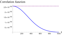
	[a] The midpoint of $X$ and $Y$ is $x=X_{f}^{1}$.
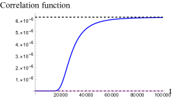
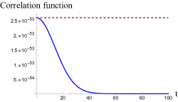
	[b] The midpoint of $X$ and $Y$ is $x=\frac{L}{4}$.
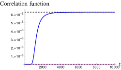
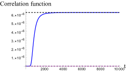
	[c] The midpoint of $X$ and $Y$ is $x=X_{f}^{2}$.

Figure 21: The time evolution of the two-point correlation function after the SSD quench when the midpoint of $X$ and $Y$ is [a]$x=X^{1}_{f}$, [b]$x=\frac{L}{4}$; [c]$x=X^{2}_{f}$. We set $h(=\overline{h})=1$.

The Möbius quench

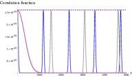
	[a] The midpoint of $X$ and $Y$ is $x=X_{f}^{1}$.
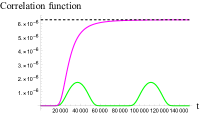
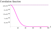
	[b] The midpoint of $X$ and $Y$ is $x=\frac{L}{4}$.
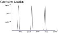
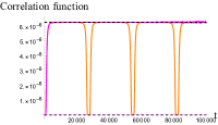
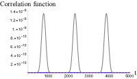
	[c] The midpoint of $X$ and $Y$ is $x=X_{f}^{2}$.

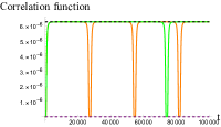
Figure 22: The time evolution of the two-point correlation function after the Möbius quench when the midpoint of $X$ and $Y$ is [a] $x=X^{1}_{f}$, [b]$x=\frac{L}{4}$, [c]$x=X^{2}_{f}$. We set $h(=\overline{h})=1$.

We show the time evolution of this two-point correlation function after the Möbius quench in Fig. 22. In this figure, we study the $\theta$ dependence of the time evolution of the two-point correlation function. The common property of these correlation functions is that they behave periodically with period $2\pi/\Omega$.

Let us elaborate on the $\theta$-dependence of the time evolution of the two-point correlation function for each case [a-c]. We will assume $L>X>\frac{3L}{4}$ and $\frac{L}{4}>Y>0$ for [a], $\frac{L}{2}>X>\frac{L}{4}$ for [b], and $\frac{L}{4}>Y>0$ for [c], respectively.

For [a], if the parameter $\theta$ is sufficiently small, the two-point correlation function becomes smaller by the Möbius time evolution from the thermal state value, and takes a minimum value. After taking that, it increases and returns to the initial state value, that is, the thermal state value. Namely, the two-point correlation function undergoes the periodic oscillation. On the other hand, if $\theta$ is sufficiently large, the two-point correlation function decreases in time evolution from the initial value, takes a minimum value, and after that, increases to reach the maximum value, which is in-between the initial and vacuum state values. After reaching the maximum, the value of the two-point correlation function decreases and returns to the initial value. These behaviors can be understood in terms of the geodesics: when $\theta$ is small, the positions of the operators are not mapped by the Möbius time evolution to the region where the geodesic becomes shorter with time, $0<Y^{\text{new}}<\frac{L}{4}$ and $\frac{L}{2}<X^{\text{new}}<\frac{3L}{4}$. On the other hand, when $\theta$ is large, they are mapped to this region. The initial positions of the operators and $\theta$ determine whether the two-point correlation function is larger than the thermal value.

Similar discussion applies to the cases [b] and [c]. For [b] when the parameter $\theta$ is sufficiently small, the two-point correlation function decreases from the thermal value, takes a minimum value, then increases and reaches a maximum value. The maximum value is in-between the initial and the vacuum state values, and determined by $\theta$; if $\theta$ is sufficiently large, the maximum is closer to the vacuum state value. After that, it then decreases and returns to the initial value. For [c], the two-point correlation function increases with time from the initial value, hits a maximum value, and then decreases to return to the initial value. This maximum value depends on $\theta$, and the larger $\theta$ is, the closer the maximum value is to the vacuum value. This is because in the case of [c], the Möbius time evolution operator maps the operator positions to the region where the geodesic length monotonically decreases, $\frac{L}{4}<Y^{\text{new}}<\frac{L}{2}$ and $\frac{L}{2}<X^{\text{new}}<\frac{3L}{4}$.

D.1.2 Operators inserted at $x=X_{f}^{1}$ and another point

We now study the local correlations between the fixed point $x=X^{f}_{1}$ and the other points by looking at the two-point correlation function between $x=X$ and $x=X_{f}^{1}$. We assume that $X>X^{1}_{f}$. As before, the two-point correlation function is initially ($t\approx 0$) given by the two-point correlation function of the thermal state.

SSD quench

When the state is quenched by the SSD Hamiltonian and enough time has passed, the two-point correlation function is given by

$$\left\langle\mathcal{O}(w_{1},\overline{w}_{1})\mathcal{O}(w_{2},\overline{w}_{2})\right\rangle\approx C_{0}\cdot\frac{\pi^{2}e^{\frac{-\pi L}{\epsilon}}}{\epsilon^{2}t^{2}\sin^{4}{\left(\frac{\pi X}{L}\right)}}\ll 1$$ (D.6)

Thus, the value of the two-point correlation function is very small compared to the two-point correlation of the vacuum state. Here, $C_{0}$ is a constant. This is due to the fact that geodesics become longer and longer as time evolves.

Möbius quench

The two-point correlation function behaves periodically when the state is quenched by the Möbius Hamiltonian, and its minimum value is between the thermal value and value defined by (D.6).

D.2 The Free fermion CFT

In this section, the two-point function of the energy density operator in the free Majorana Fermion CFT after the SSD/Möbius quench is computed. The energy density can be written in terms of the Majorana spinors as $\varepsilon=i\psi\bar{\psi}$ [101]. This is a spinless non-chiral field with $h=\bar{h}=\frac{1}{2}$ and is proportional to the mass term $m\psi\bar{\psi}$ [101]. Note that $\varepsilon^{\dagger}=\varepsilon$ because the Majorana spinors are real [134]. The two-point energy correlator on the complex plane is given by [101]

$$\langle\varepsilon(z,\bar{z})\varepsilon(0,0)\rangle_{\nu}=\left|\wp_{\nu}(z)\right|^{2}$$ (D.7)

where we introduced the function [101]

$$\wp_{\nu}(z)=\frac{\vartheta_{\nu}(z|\tau)\partial_{z}\vartheta_{1}(0|\tau)}{\vartheta_{\nu}(0|\tau)\vartheta_{1}(z|\tau)}\qquad(\nu=2,3,4)$$ (D.8)

Since the first elliptic theta function is odd with respect to $z$ while the other three are even functions of $z$, this function is odd with respect to $z$, i.e. $\wp_{\nu}(-z)=-\wp_{\nu}(z)$. Under a generic Mobius evolution (including the SSD limit), the two-point function on the torus evolves as

$$\langle\varepsilon(w_{X_{1}},\bar{w}_{X_{1}})\varepsilon(w_{X_{2}},\bar{w}_{X_{2}})\rangle_{\nu}= \left(\frac{1}{2\epsilon}\right)^{2}\prod_{i=1,2}\left(\frac{dw_{X_{i}}^{\text{new}}}{dw_{X_{i}}}\frac{d\bar{w}_{X_{i}}^{\text{new}}}{d\bar{w}_{X_{i}}}\right)^{h}\left\langle\varepsilon\left(\frac{w_{X_{1}}^{\text{new}}}{2\epsilon},\frac{\bar{w}_{X_{1}}^{\text{new}}}{2\epsilon}\right)\varepsilon\left(\frac{w_{X_{2}}^{\text{new}}}{2\epsilon},\frac{\bar{w}_{X_{2}}^{\text{new}}}{2\epsilon}\right)\right\rangle_{\nu}$$

$$= \left(\frac{1}{2\epsilon}\right)^{2}\prod_{i=1,2}\left(\frac{dw_{X_{i}}^{\text{new}}}{dw_{X_{i}}}\frac{d\bar{w}_{X_{i}}^{\text{new}}}{d\bar{w}_{X_{i}}}\right)^{h}\left|\frac{\vartheta_{\nu}\left(\frac{w_{X_{1}}^{\text{new}}-w_{X_{2}}^{\text{new}}}{2\epsilon}\bigg{|}\tau\right)\partial_{z}\vartheta_{1}(0|\tau)}{\vartheta_{\nu}(0|\tau)\vartheta_{1}\left(\frac{w_{X_{1}}^{\text{new}}-w_{X_{2}}^{\text{new}}}{2\epsilon}\bigg{|}\tau\right)}\right|^{2}$$ (D.9)

where the first conformal factor comes from rescaling the torus coordinates so as to have periods $1$ and $\tau$ and the second conformal factor comes from evolving the operator in the Heisenberg picture.

The two point function is plotted in Fig. 23. for the cases where the midpoint between the two operators is located at $x=0,\frac{L}{4}$ and $\frac{L}{2}$. Only the results for the physical boundary conditions $\nu=3,4$ are shown, and they are identical. The results are similar to those in the holographic CFT. Since the initial state is the thermal one, the two-point correlation function starts at the thermal value. In the first two cases, the two-point correlator decreases initially. Eventually, the two-point correlation function increases and saturates at the value of the corresponding vacuum two-point function. This is reminiscent of the behavior of mutual information which began at the thermal value and saturated at the mutual information of the uniform ground state. Another point worth noting is that as the two-point correlation function is moved away from the stable fixed point towards the unstable fixed point, the correlation function saturates faster. In fact, when the two-point correlation function is situated such that the midway point sits on the unstable fixed point, it does not decrease at all and simply grows from the thermal value to that of the vacuum correlation function.

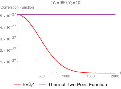
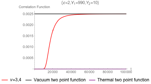
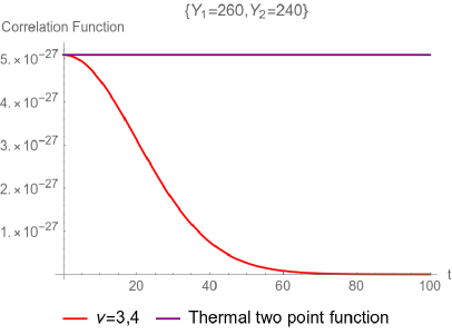
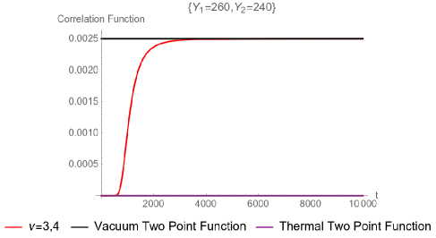
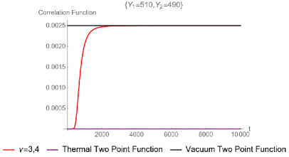
Figure 23: The energy density two point function (D.2) after the SSD quench. The total system size is $L=1000$. The top, middle and bottom row corresponds to placing the two operators such that the midpoint between the two operators lies at $x=0,\frac{L}{4}$ and $\frac{L}{2}$, respectively. The regulator is set to $\epsilon=1$ except for the top right plot where $\epsilon=2$. The black and purple lines are the values of the correlation function in the thermal and vacuum state, respectively.

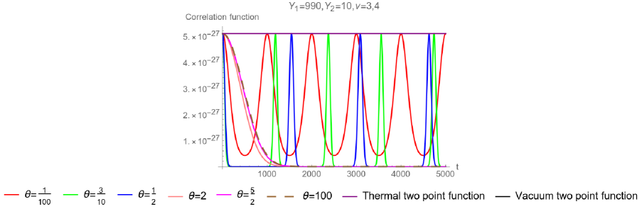
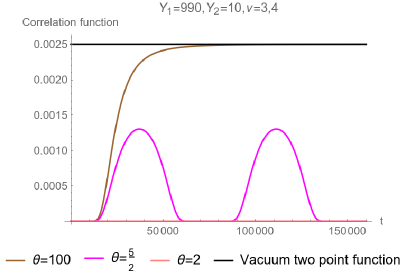
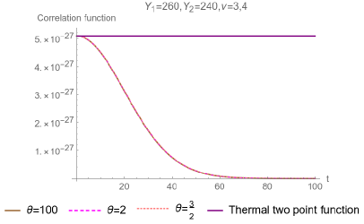
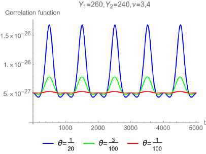
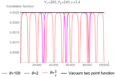
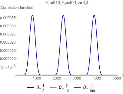
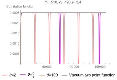
Figure 24: The energy density two-point correlation function of the Majoran fermion theory (D.2). The total system size is set to $L=1000$ and the regulator is $\epsilon=1$. The black and purple lines correspond to the same correlation function evaluated in the thermal and uniform vacuum state respectively.

Plots of the free fermion two-point energy density correlation function under a Möbius quench (D.2) are shown in Fig. 24. These results are very similar to the holographic case. For small values of the deformation parameter $\theta<1$, the two-point correlation function simply oscillates and returns to the initial thermal value with periods given by $L\cosh 2\theta$. As the deformation parameter increases, the amplitude and period of the correlation function increases until it approaches the SSD case. Also, as the pair of operators are moved away from the stable fixed point of the SSD Hamiltonian, the correlation function saturates faster.

D.3 Validity of the approximation of (1.7)

Here, we show that the time evolution of the two-point correlation function after $H_{{\rm SSD}}$ can be adequately explained by the approximation of (1.7) at late enough times. First, for operators inserted other than $X^{1}_{f}$, we see that from (1.7), the reduced density matrix for the subsystem excluding $\mathcal{V}$ is the reduced density matrix for the vacuum state. So (1.7) reproduces the behavior of the two-point correlation function. On the other hand, when one of the operators is inserted at $x=X^{1}_{f}$, (1.7) suggests $\left\langle\mathcal{O}(X_{f}^{1})\mathcal{O}(x\neq X_{f}^{1})\right\rangle\approx\text{tr}_{A}\left(\rho_{A}\mathcal{O}(X_{f}^{1})\right)\cdot\left<0\right|\mathcal{O}(x\neq X_{f}^{1})\left|0\right>=0$ where we noted the vacuum expectation value of the operator is $0$. Thus, the late time approximation (1.7) fully reproduces the result (D.6), in which the two-point correlation function is very small.

References

- [1] J. M. Deutsch, “Quantum statistical mechanics in a closed system,” Phys. Rev. A, vol. 43, pp. 2046–2049, Feb 1991.
- [2] M. Srednicki, “Chaos and quantum thermalization,” Physical Review E, vol. 50, pp. 888–901, Aug 1994.
- [3] D. Basko, I. Aleiner, and B. Altshuler, “Metal–insulator transition in a weakly interacting many-electron system with localized single-particle states,” Annals of Physics, vol. 321, pp. 1126–1205, May 2006.
- [4] M. Serbyn, Z. Papić, and D. A. Abanin, “Local conservation laws and the structure of the many-body localized states,” Physical Review Letters, vol. 111, Sep 2013.
- [5] D. A. Huse, R. Nandkishore, and V. Oganesyan, “Phenomenology of fully many-body-localized systems,” Physical Review B, vol. 90, Nov 2014.
- [6] R. Nandkishore and D. A. Huse, “Many-body localization and thermalization in quantum statistical mechanics,” Annual Review of Condensed Matter Physics, vol. 6, pp. 15–38, Mar 2015.
- [7] H. Bernien, S. Schwartz, A. Keesling, H. Levine, A. Omran, H. Pichler, S. Choi, A. S. Zibrov, M. Endres, M. Greiner, V. Vuletić, and M. D. Lukin, “Probing many-body dynamics on a 51-atom quantum simulator,” Nov. 2017.
- [8] C. J. Turner, A. A. Michailidis, D. A. Abanin, M. Serbyn, and Z. Papić, “Quantum scarred eigenstates in a Rydberg atom chain: Entanglement, breakdown of thermalization, and stability to perturbations,” Phys. Rev. B, vol. 98, p. 155134, Oct. 2018.
- [9] S. Moudgalya, N. Regnault, and B. A. Bernevig, “Entanglement of Exact Excited States of AKLT Models: Exact Results, Many-Body Scars and the Violation of Strong ETH,” arXiv e-prints, p. arXiv:1806.09624, June 2018.
- [10] C.-J. Lin and O. I. Motrunich, “Exact quantum many-body scar states in the rydberg-blockaded atom chain,” Physical Review Letters, vol. 122, Apr 2019.
- [11] W. W. Ho, S. Choi, H. Pichler, and M. D. Lukin, “Periodic Orbits, Entanglement, and Quantum Many-Body Scars in Constrained Models: Matrix Product State Approach,” Phys. Rev. Lett., vol. 122, no. 4, p. 040603, 2019.
- [12] C. J. Turner, A. A. Michailidis, D. A. Abanin, M. Serbyn, Papić, and Z. , “Weak ergodicity breaking from quantum many-body scars,” Nature Physics, vol. 14, pp. 745–749, May 2018.
- [13] Z. Papić, “Weak ergodicity breaking through the lens of quantum entanglement,” arXiv e-prints, p. arXiv:2108.03460, Aug. 2021.
- [14] S. Moudgalya, B. A. Bernevig, and N. Regnault, “Quantum Many-Body Scars and Hilbert Space Fragmentation: A Review of Exact Results,” arXiv e-prints, p. arXiv:2109.00548, Sept. 2021.
- [15] S. W. Hawking, “Particle creation by black holes,” Communications in Mathematical Physics, vol. 43, pp. 199–220, Aug. 1975.
- [16] D. N. Page, “Information in black hole radiation,” Physical Review Letters, vol. 71, pp. 3743–3746, Dec 1993.
- [17] A. Almheiri, N. Engelhardt, D. Marolf, and H. Maxfield, “The entropy of bulk quantum fields and the entanglement wedge of an evaporating black hole,” Journal of High Energy Physics, vol. 2019, Dec 2019.
- [18] G. Penington, “Entanglement Wedge Reconstruction and the Information Paradox,” JHEP, vol. 09, p. 002, 2020.
- [19] A. Almheiri, R. Mahajan, J. Maldacena, and Y. Zhao, “The page curve of hawking radiation from semiclassical geometry,” Journal of High Energy Physics, vol. 2020, Mar 2020.
- [20] A. Almheiri, T. Hartman, J. Maldacena, E. Shaghoulian, and A. Tajdini, “Replica wormholes and the entropy of hawking radiation,” Journal of High Energy Physics, vol. 2020, May 2020.
- [21] G. Penington, S. H. Shenker, D. Stanford, and Z. Yang, “Replica wormholes and the black hole interior,” 11 2019.
- [22] K. Goto, T. Hartman, and A. Tajdini, “Replica wormholes for an evaporating 2D black hole,” JHEP, vol. 04, p. 289, 2021.
- [23] P. Calabrese and J. Cardy, “Evolution of entanglement entropy in one-dimensional systems,” Journal of Statistical Mechanics: Theory and Experiment, vol. 4, p. 04010, Apr. 2005.
- [24] P. Calabrese and J. Cardy, “Entanglement and correlation functions following a local quench: a conformal field theory approach,” Journal of Statistical Mechanics: Theory and Experiment, vol. 2007, pp. P10004–P10004, Oct 2007.
- [25] F. C. Alcaraz, M. I. Berganza, and G. Sierra, “Entanglement of low-energy excitations in conformal field theory,” Physical Review Letters, vol. 106, May 2011.
- [26] M. Nozaki, T. Numasawa, and T. Takayanagi, “Quantum entanglement of local operators in conformal field theories,” Physical Review Letters, vol. 112, Mar 2014.
- [27] R. Islam, R. Ma, P. M. Preiss, M. E. Tai, A. Lukin, M. Rispoli, and M. Greiner, “Measuring entanglement entropy through the interference of quantum many-body twins,” arXiv e-prints, p. arXiv:1509.01160, Sep 2015.
- [28] A. Lukin, M. Rispoli, R. Schittko, M. E. Tai, A. M. Kaufman, S. Choi, V. Khemani, J. Léonard, and M. Greiner, “Probing entanglement in a many-body-localized system,” Science, vol. 364, pp. 256–260, Apr 2019.
- [29] T. Brydges, A. Elben, P. Jurcevic, B. Vermersch, C. Maier, B. P. Lanyon, P. Zoller, R. Blatt, and C. F. Roos, “Probing Rényi entanglement entropy via randomized measurements,” Science, vol. 364, pp. 260–263, Apr 2019.
- [30] S. Sotiriadis and J. Cardy, “Inhomogeneous Quantum Quenches,” J. Stat. Mech., vol. 0811, p. P11003, 2008.
- [31] P. Calabrese and J. Cardy, “Quantum quenches in 1 + 1 dimensional conformal field theories,” J. Stat. Mech., vol. 1606, no. 6, p. 064003, 2016.
- [32] X. Wen, “Bridging global and local quantum quenches in conformal field theories,” 10 2016.
- [33] J. Dubail, J.-M. Stéphan, J. Viti, and P. Calabrese, “Conformal Field Theory for Inhomogeneous One-dimensional Quantum Systems: the Example of Non-Interacting Fermi Gases,” SciPost Phys., vol. 2, no. 1, p. 002, 2017.
- [34] V. Alba, B. Bertini, M. Fagotti, L. Piroli, and P. Ruggiero, “Generalized-hydrodynamic approach to inhomogeneous quenches: correlations, entanglement and quantum effects,” J. Stat. Mech., vol. 2111, p. 114004, 2021.
- [35] D. X. Horváth, M. Kormos, S. Sotiriadis, and G. Takács, “Inhomogeneous quantum quenches in the sine-Gordon theory,” 9 2021.
- [36] T. Ugajin, “Two dimensional quantum quenches and holography,” 11 2013.
- [37] V. Balasubramanian, A. Bernamonti, J. de Boer, B. Craps, L. Franti, F. Galli, E. Keski-Vakkuri, B. Müller, and A. Schäfer, “Inhomogeneous holographic thermalization,” JHEP, vol. 10, p. 082, 2013.
- [38] V. Balasubramanian, A. Bernamonti, J. de Boer, B. Craps, L. Franti, F. Galli, E. Keski-Vakkuri, B. Müller, and A. Schäfer, “Inhomogeneous Thermalization in Strongly Coupled Field Theories,” Phys. Rev. Lett., vol. 111, p. 231602, 2013.
- [39] K. A. Sohrabi, “Inhomogeneous thermal quenches,” Phys. Rev. D, vol. 96, p. 026012, Jul 2017.
- [40] I. Y. Aref’eva, M. A. Khramtsov, and M. D. Tikhanovskaya, “Thermalization after holographic bilocal quench,” JHEP, vol. 09, p. 115, 2017.
- [41] T. De Jonckheere and J. Lindgren, “Entanglement entropy in inhomogeneous quenches in AdS3/CFT2,” Phys. Rev. D, vol. 98, no. 10, p. 106006, 2018.
- [42] J. Kudler-Flam, Y. Kusuki, and S. Ryu, “Correlation measures and the entanglement wedge cross-section after quantum quenches in two-dimensional conformal field theories,” JHEP, vol. 04, p. 074, 2020.
- [43] A. Gendiar, R. Krcmar, and T. Nishino, “Spherical deformation for one-dimensional quantum systems,” Progress of Theoretical Physics, vol. 122, no. 4, pp. 953–967, 2009.
- [44] A. Gendiar, R. Krcmar, and T. Nishino, “Spherical deformation for one-dimensional quantum systems,” Progress of Theoretical Physics, vol. 123, no. 2, p. 393, 2010.
- [45] T. Hikihara and T. Nishino, “Connecting distant ends of one-dimensional critical systems by a sine-square deformation,” Physical Review B, vol. 83, Feb 2011.
- [46] A. Gendiar, M. Daniška, Y. Lee, and T. Nishino, “Suppression of finite-size effects in one-dimensional correlated systems,” Phys. Rev. A, vol. 83, p. 052118, May 2011.
- [47] K. Okunishi, “Sine-square deformation and möbius quantization of 2d conformal field theory,” Progress of Theoretical and Experimental Physics, vol. 2016, p. 063A02, Jun 2016.
- [48] X. Wen, S. Ryu, and A. W. W. Ludwig, “Evolution operators in conformal field theories and conformal mappings: Entanglement Hamiltonian, the sine-square deformation, and others,” Phys. Rev. B, vol. 93, p. 235119, June 2016.
- [49] N. Shibata and C. Hotta, “Boundary effects in the density-matrix renormalization group calculation,” Phys. Rev. B, vol. 84, p. 115116, Sept. 2011.
- [50] I. Maruyama, H. Katsura, and T. Hikihara, “Sine-square deformation of free fermion systems in one and higher dimensions,” Phys. Rev. B, vol. 84, p. 165132, Oct. 2011.
- [51] H. Katsura, “Exact ground state of the sine-square deformed XY spin chain,” Journal of Physics A Mathematical General, vol. 44, p. 252001, June 2011.
- [52] H. Katsura, “Sine-square deformation of solvable spin chains and conformal field theories,” Journal of Physics A Mathematical General, vol. 45, p. 115003, Mar. 2012.
- [53] C. Hotta and N. Shibata, “Grand canonical finite-size numerical approaches: A route to measuring bulk properties in an applied field,” Phys. Rev. B, vol. 86, p. 041108, Jul 2012.
- [54] C. Hotta, S. Nishimoto, and N. Shibata, “Grand canonical finite size numerical approaches in one and two dimensions: Real space energy renormalization and edge state generation,” Phys. Rev. B, vol. 87, p. 115128, Mar 2013.
- [55] T. Tada, “Sine-square deformation and its relevance to string theory,” Modern Physics Letters A, vol. 30, p. 1550092, May 2015.
- [56] N. Ishibashi and T. Tada, “Infinite circumference limit of conformal field theory,” Journal of Physics A Mathematical General, vol. 48, p. 315402, Aug. 2015.
- [57] N. Ishibashi and T. Tada, “Dipolar quantization and the infinite circumference limit of two-dimensional conformal field theories,” International Journal of Modern Physics A, vol. 31, p. 1650170, Nov. 2016.
- [58] X. Wen and J.-Q. Wu, “Quantum dynamics in sine-square deformed conformal field theory: Quench from uniform to nonuniform conformal field theory,” Physical Review B, vol. 97, May 2018.
- [59] X. Wen and J.-Q. Wu, “Floquet conformal field theory,” 2018.
- [60] R. Fan, Y. Gu, A. Vishwanath, and X. Wen, “Emergent spatial structure and entanglement localization in floquet conformal field theory,” Physical Review X, vol. 10, Aug 2020.
- [61] B. Han and X. Wen, “Classification of sl2 deformed floquet conformal field theories,” Physical Review B, vol. 102, Nov 2020.
- [62] X. Wen, R. Fan, A. Vishwanath, and Y. Gu, “Periodically, quasi-periodically, and randomly driven conformal field theories: Part i,” 2021.
- [63] R. Fan, Y. Gu, A. Vishwanath, and X. Wen, “Floquet conformal field theories with generally deformed hamiltonians,” SciPost Physics, vol. 10, Feb 2021.
- [64] B. Lapierre, K. Choo, A. Tiwari, C. Tauber, T. Neupert, and R. Chitra, “Fine structure of heating in a quasiperiodically driven critical quantum system,” Physical Review Research, vol. 2, Sep 2020.
- [65] B. Lapierre, K. Choo, C. Tauber, A. Tiwari, T. Neupert, and R. Chitra, “Emergent black hole dynamics in critical floquet systems,” Physical Review Research, vol. 2, Apr 2020.
- [66] S. Sotiriadis, P. Calabrese, and J. Cardy, “Quantum quench from a thermal initial state,” EPL (Europhysics Letters), vol. 87, p. 20002, Jul 2009.
- [67] N. T. Jacobson, L. C. Venuti, and P. Zanardi, “Unitary equilibration after a quantum quench of a thermal state,” Physical Review A, vol. 84, Aug 2011.
- [68] K. A. Sohrabi, “Inhomogeneous Thermal Quenches,” arXiv e-prints, p. arXiv:1509.00245, Sept. 2015.
- [69] M. P. Zaletel, A. M. Kaufman, D. M. Stamper-Kurn, and N. Y. Yao, “Preparation of Low Entropy Correlated Many-body States via Conformal Cooling Quenches,” arXiv e-prints, p. arXiv:1611.04591, Nov. 2016.
- [70] P. Mitra, M. Ippoliti, R. N. Bhatt, S. L. Sondhi, and K. Agarwal, “Cooling arbitrary near-critical systems using hyperbolic quenches,” Phys. Rev. B, vol. 99, p. 104308, Mar. 2019.
- [71] H. Liu and S. J. Suh, “Entanglement Tsunami: Universal Scaling in Holographic Thermalization,” Phys. Rev. Lett., vol. 112, p. 011601, 2014.
- [72] H. Liu and S. J. Suh, “Entanglement growth during thermalization in holographic systems,” Phys. Rev. D, vol. 89, no. 6, p. 066012, 2014.
- [73] C. T. Asplund and A. Bernamonti, “Mutual information after a local quench in conformal field theory,” Phys. Rev. D, vol. 89, no. 6, p. 066015, 2014.
- [74] P. Caputa, M. Nozaki, and T. Takayanagi, “Entanglement of local operators in large-N conformal field theories,” PTEP, vol. 2014, p. 093B06, 2014.
- [75] C. T. Asplund, A. Bernamonti, F. Galli, and T. Hartman, “Holographic Entanglement Entropy from 2d CFT: Heavy States and Local Quenches,” JHEP, vol. 02, p. 171, 2015.
- [76] C. T. Asplund, A. Bernamonti, F. Galli, and T. Hartman, “Entanglement Scrambling in 2d Conformal Field Theory,” JHEP, vol. 09, p. 110, 2015.
- [77] P. Hosur, X.-L. Qi, D. A. Roberts, and B. Yoshida, “Chaos in quantum channels,” JHEP, vol. 02, p. 004, 2016.
- [78] A. Nahum, J. Ruhman, S. Vijay, and J. Haah, “Quantum entanglement growth under random unitary dynamics,” Phys. Rev. X, vol. 7, p. 031016, Jul 2017.
- [79] C. Jonay, D. A. Huse, and A. Nahum, “Coarse-grained dynamics of operator and state entanglement,” 2018.
- [80] L. Nie, M. Nozaki, S. Ryu, and M. T. Tan, “Signature of quantum chaos in operator entanglement in 2d CFTs,” J. Stat. Mech., vol. 1909, no. 9, p. 093107, 2019.
- [81] J. Kudler-Flam, M. Nozaki, S. Ryu, and M. T. Tan, “Quantum vs. classical information: operator negativity as a probe of scrambling,” JHEP, vol. 01, p. 031, 2020.
- [82] J. Kudler-Flam, M. Nozaki, S. Ryu, and M. T. Tan, “Entanglement of local operators and the butterfly effect,” Phys. Rev. Res., vol. 3, no. 3, p. 033182, 2021.
- [83] J. Kudler-Flam, Y. Kusuki, and S. Ryu, “The quasi-particle picture and its breakdown after local quenches: mutual information, negativity, and reflected entropy,” JHEP, vol. 03, p. 146, 2021.
- [84] B. Freivogel, J. McGreevy, and S. J. Suh, “Exactly stable collective oscillations in conformal field theory,” Physical Review D, vol. 85, May 2012.
- [85] B. G. Chowdhury, S. Datta, and J. R. David, “Rényi divergences from Euclidean quenches,” Journal of High Energy Physics, vol. 2020, p. 94, Apr. 2020.
- [86] J. H. Eberly, N. B. Narozhny, and J. J. Sanchez-Mondragon, “Periodic spontaneous collapse and revival in a simple quantum model,” Phys. Rev. Lett., vol. 44, pp. 1323–1326, May 1980.
- [87] Z. D. c. v. a. c. Gaeta and C. R. Stroud, “Classical and quantum-mechanical dynamics of a quasiclassical state of the hydrogen atom,” Phys. Rev. A, vol. 42, pp. 6308–6313, Dec 1990.
- [88] M. Haque and J. M. Zhang, “Nonsmooth and level-resolved dynamics illustrated with a periodically driven tight binding model,” ScienceOpen Research, Dec 2014.
- [89] P. Calabrese and J. Cardy, “Entanglement entropy and quantum field theory,” Journal of Statistical Mechanics: Theory and Experiment, vol. 2004, p. P06002, Jun 2004.
- [90] P. Calabrese and J. Cardy, “Entanglement entropy and conformal field theory,” Journal of Physics A: Mathematical and Theoretical, vol. 42, p. 504005, Dec 2009.
- [91] S. W. Hawking and D. N. Page, “Thermodynamics of black holes in anti-de sitter space,” Communications in Mathematical Physics, vol. 87, no. 4, pp. 577–588, 1983.
- [92] S. Ryu and T. Takayanagi, “Holographic derivation of entanglement entropy from the anti–de sitter space/conformal field theory correspondence,” Physical Review Letters, vol. 96, May 2006.
- [93] M. Headrick, “General properties of holographic entanglement entropy,” Journal of High Energy Physics, vol. 2014, Mar 2014.
- [94] L. Susskind, “The World as a hologram,” J. Math. Phys., vol. 36, pp. 6377–6396, 1995.
- [95] G. ’t Hooft, “Dimensional reduction in quantum gravity,” Conf. Proc. C, vol. 930308, pp. 284–296, 1993.
- [96] J. D. Bekenstein, “Black holes and entropy,” Phys. Rev. D, vol. 7, pp. 2333–2346, 1973.
- [97] S. W. Hawking, “Particle Creation by Black Holes,” Commun. Math. Phys., vol. 43, pp. 199–220, 1975. [Erratum: Commun.Math.Phys. 46, 206 (1976)].
- [98] G. W. Gibbons and S. W. Hawking, “Action Integrals and Partition Functions in Quantum Gravity,” Phys. Rev. D, vol. 15, pp. 2752–2756, 1977.
- [99] P. Calabrese and J. Cardy, “Entanglement and correlation functions following a local quench: a conformal field theory approach,” Journal of Statistical Mechanics: Theory and Experiment, vol. 10, p. 10004, Oct. 2007.
- [100] S. Datta, P. Kraus, and B. Michel, “Typicality and thermality in 2d CFT,” JHEP, vol. 07, p. 143, 2019.
- [101] P. Di Francesco, P. Mathieu, and D. Sénéchal, Conformal Field Theory. Graduate texts in contemporary physics, Island Press, 1996.
- [102] S. He and Y. Sun, “Correlation functions of cfts on a torus with a deformation,” Phys. Rev. D, vol. 102, p. 026023, Jul 2020.
- [103] C. P. Herzog and T. Nishioka, “Entanglement entropy of a massive fermion on a torus,” Journal of High Energy Physics, vol. 2013, p. 77, Mar 2013.
- [104] M. Bañados, “Three-dimensional quantum geometry and black holes,” 1999.
- [105] M. M. Roberts, “Time evolution of entanglement entropy from a pulse,” JHEP, vol. 12, p. 027, 2012.
- [106] I. MacCormack, A. Liu, M. Nozaki, and S. Ryu, “Holographic duals of inhomogeneous systems: the rainbow chain and the sine-square deformation model,” Journal of Physics A: Mathematical and Theoretical, vol. 52, p. 505401, Nov 2019.
- [107] K. Goto and T. Takayanagi, “CFT descriptions of bulk local states in the AdS black holes,” JHEP, vol. 10, p. 153, 2017.
- [108] S. Ryu and T. Takayanagi, “Aspects of holographic entanglement entropy,” Journal of High Energy Physics, vol. 8, p. 045, Aug. 2006.
- [109] S. Furukawa, V. Pasquier, and J. Shiraishi, “Mutual information and boson radius in a critical system in one dimension,” Phys. Rev. Lett., vol. 102, p. 170602, Apr 2009.
- [110] A. Keesling, A. Omran, H. Levine, H. Bernien, H. Pichler, S. Choi, R. Samajdar, S. Schwartz, P. Silvi, S. Sachdev, P. Zoller, M. Endres, M. Greiner, Vuletić, V. , and M. D. Lukin, “Quantum Kibble-Zurek mechanism and critical dynamics on a programmable Rydberg simulator,” Nature, vol. 568, pp. 207–211, Apr. 2019.
- [111] K. Slagle, D. Aasen, H. Pichler, R. S. K. Mong, P. Fendley, X. Chen, M. Endres, and J. Alicea, “Microscopic characterization of Ising conformal field theory in Rydberg chains,” arXiv e-prints, p. arXiv:2108.09309, Aug. 2021.
- [112] Y. Li, X. Chen, and M. P. A. Fisher, “Quantum zeno effect and the many-body entanglement transition,” Physical Review B, vol. 98, Nov 2018.
- [113] A. Chan, R. M. Nandkishore, M. Pretko, and G. Smith, “Unitary-projective entanglement dynamics,” Physical Review B, vol. 99, Jun 2019.
- [114] B. Skinner, J. Ruhman, and A. Nahum, “Measurement-induced phase transitions in the dynamics of entanglement,” Physical Review X, vol. 9, Jul 2019.
- [115] Y. Li, X. Chen, and M. P. A. Fisher, “Measurement-driven entanglement transition in hybrid quantum circuits,” Physical Review B, vol. 100, Oct 2019.
- [116] X. Chen, Y. Li, M. P. A. Fisher, and A. Lucas, “Emergent conformal symmetry in nonunitary random dynamics of free fermions,” Physical Review Research, vol. 2, Jul 2020.
- [117] M. J. Gullans and D. A. Huse, “Dynamical Purification Phase Transition Induced by Quantum Measurements,” Phys. Rev. X, vol. 10, no. 4, p. 041020, 2020.
- [118] M. Ippoliti, M. J. Gullans, S. Gopalakrishnan, D. A. Huse, and V. Khemani, “Entanglement Phase Transitions in Measurement-Only Dynamics,” Physical Review X, vol. 11, p. 011030, Jan. 2021.
- [119] Y. Li and M. P. A. Fisher, “Statistical mechanics of quantum error correcting codes,” Phys. Rev. B, vol. 103, p. 104306, Mar. 2021.
- [120] B. Yoshida, “Decoding the Entanglement Structure of Monitored Quantum Circuits,” 9 2021.
- [121] S. Åminneborg, I. Bengtsson, and S. Holst, “A spinning anti-de Sitter wormhole,” Classical and Quantum Gravity, vol. 16, pp. 363–382, Feb. 1999.
- [122] E. Chitambar, D. Leung, L. Mančinska, M. Ozols, and A. Winter, “Everything you always wanted to know about locc (but were afraid to ask),” Communications in Mathematical Physics, vol. 328, pp. 303–326, Mar 2014.
- [123] B. Czech, J. L. Karczmarek, F. Nogueira, and M. Van Raamsdonk, “The gravity dual of a density matrix,” Classical and Quantum Gravity, vol. 29, p. 155009, Jul 2012.
- [124] A. C. Wall, “Maximin surfaces, and the strong subadditivity of the covariant holographic entanglement entropy,” Classical and Quantum Gravity, vol. 31, p. 225007, Nov 2014.
- [125] M. Headrick, V. E. Hubeny, A. Lawrence, and M. Rangamani, “Causality \& holographic entanglement entropy,” JHEP, vol. 12, p. 162, 2014.
- [126] D. L. Jafferis and S. J. Suh, “The Gravity Duals of Modular Hamiltonians,” JHEP, vol. 09, p. 068, 2016.
- [127] M. C. Bañuls, J. I. Cirac, and M. B. Hastings, “Strong and weak thermalization of infinite nonintegrable quantum systems,” Physical Review Letters, vol. 106, Feb 2011.
- [128] A. Nahum, J. Ruhman, S. Vijay, and J. Haah, “Quantum Entanglement Growth under Random Unitary Dynamics,” Physical Review X, vol. 7, p. 031016, July 2017.
- [129] C. W. von Keyserlingk, T. Rakovszky, F. Pollmann, and S. L. Sondhi, “Operator Hydrodynamics, OTOCs, and Entanglement Growth in Systems without Conservation Laws,” Physical Review X, vol. 8, p. 021013, Apr 2018.
- [130] C. Jonay, D. A. Huse, and A. Nahum, “Coarse-grained dynamics of operator and state entanglement,” arXiv e-prints, p. arXiv:1803.00089, Feb 2018.
- [131] M. Mezei, “Membrane theory of entanglement dynamics from holography,” Phys. Rev. D, vol. 98, p. 106025, Nov. 2018.
- [132] V. Balasubramanian and S. F. Ross, “Holographic particle detection,” Physical Review D, vol. 61, Jan 2000.
- [133] E. Keski-Vakkuri, “Bulk and boundary dynamics in btz black holes,” Physical Review D, vol. 59, Mar 1999.
- [134] R. Blumenhagen and E. Plauschinn, Introduction to Conformal Field Theory: With Applications to String Theory. Lecture Notes in Physics, Springer Berlin Heidelberg, 2009.