Reconstructing the exit wave in high-resolution transmission electron microscopy using machine learning

Abstract

Reconstruction of the exit wave function is an important route to interpreting high-resolution transmission electron microscopy (HRTEM) images. Here we demonstrate that convolutional neural networks can be used to reconstruct the exit wave from a short focal series of HRTEM images, with a fidelity comparable to conventional exit wave reconstruction. We use a fully convolutional neural network based on the U-Net architecture, and demonstrate that we can train it on simulated exit waves and simulated HRTEM images of graphene-supported molybdenum disulphide (an industrial desulfurization catalyst). We then apply the trained network to analyse experimentally obtained images from similar samples, and obtain exit waves that clearly show the atomically resolved structure of both the MoS₂ nanoparticles and the graphene support. We also show that it is possible to successfully train the neural networks to reconstruct exit waves for 3400 different two-dimensional materials taken from the Computational 2D Materials Database of known and proposed two-dimensional materials.

1 Introduction

Machine learning has become a powerful tool for analyzing images. In fact, machine learning is a nascent tool in electron microscopy that is envisioned to have a large potential for quantitative image analysis [1, 2]. In electron microscopy, applications of machine learning have up to now included segmentation of medical images [3], grain and phase identification [4, 5, 6], noise filtering [7, 8] and in-plane location of atoms [9, 10, 11]. Moreover, Ede et al. showed recently that the imaginary part of the exit wave function can be reconstructed from the real part using a convolutional neural network [12] and Meyer showed that off-axis holograms, where phase information is recorded directly into the image, can be reconstructed using neural networks [13]. In this work we suggest that neural networks could potentially solve the classical phase problem and thus retrieve the entire electron wave function exiting the specimen in a transmission electron microscopy experiment.

Aberration-corrected high-resolution transmission electron microscopy (HRTEM) is one of the important experimental techniques to study the structure of materials at the atomic scale. The maximal amount of information about the sample is present in the exit wave, i.e. the wavefunction of the electrons exiting the sample. As the image is formed, some of this information is lost, both due to aberration in the lenses, and because the camera detects the intensity of the wave, not its phase.

It is well established that the full exit wave can be reconstructed from a focal series of images [14, 15]. A series of typically around 20–50 images with varying defocus is used to numerically reconstruct the most likely wave function of the electron beam as it exits the sample. This can then be used to further reconstruct information about the chemical composition and 3D structure of the sample [16, 17]. For beam-sensitive samples [18], exit wave reconstruction has the advantage of being averaging in nature such that information from many images with very low signal-to-noise ratio is combined in a single exit wave image of superior signat-to-noise ratio [17]. Several numerical algorithms are available for reconstructing the exit wave [19, 20, 21].

Here we examine a Convolutional Neural Network (CNN) as an alternative way to reconstruct the exit wave. This reconstruction is possible from a low number of HRTEM images, and with the advantage that the detailed knowledge of the aberration parameters of the microscope is not needed. We envision that this can be developed into a tool for on-the-fly exit wave reconstruction while taking data on the microscope, perhaps supplemented with more traditional exit wave reconstruction as post processing. In the present case, the images were convoluted with the effects of defocus, first order astigmatism, coma, and blurring including focal spread. In this case a focal series of two to three simulated HRTEM images were sufficient to reconstruct the exit wave with sufficient accuracy in order to extract quantitative information about the sample. In principle, it should be straightforward to extend the present method to situations with low signal-to-noise ratio and more unknown aberrations, in which case it is likely that a larger focal series will be needed.

Recently, atomically thin two-dimensional (2D) materials have been an active topic of research, with applications ranging from electronics to energy storage and catalysis [22, 23]. For example, molybdenum disulphide (MoS₂) is the preferred catalyst for removing sulphur from crude oil, and is one of the reasons that acid rain is no longer one of the most pressing environmental problems [24]. In this paper, we focus on exit wave reconstruction for the rapidly growing class of 2D materials, although the methods should be generally applicable. We show that neural networks can reconstruct the exit wave both when trained to a single material, and to a database of thousands of proposed 2D materials. The reconstruction is of sufficient quality to permit analysis of the image peaks associated with the atomic columns e.g. by using Argand plots to identify the type and number of elements in the material [16].

We also show that it is possible to train the neural network purely on simulated data, and apply it successfully to experimental images of non-trivial complexity, in this case a model catalyst based on molybdenum disulphide.

2 Methods

The neural network architecture is a Unet [25] / FusionNet [3] architecture, very close to the one used by Madsen et al. [9], with the main modification that concatenation is used instead of elementwise addition for the skip connections. A linear activation function is applied in the output layer, as exit wave reconstruction is a regression problem rather than a classification/segmentation problem. Details of the architecture can be found in the Supplementary Online Information (SOI Sec. S1). The neural network is implemented and trained using the Keras interface [26] to Tensorflow version 2.5 [27]. We train using simulated images only. We computer-generate a training set and a corresponding validation set of atomic structures, using the Atomic Simulation Environment (ASE) [28].

Three data sets of increasing complexity were created. The first consists of nanoparticles (nanoflakes) of molybdenum disulphide (MoS₂). In this data set we ignore that the nanoparticles will typically be supported on another material in the microscope. Nevertheless this data set will be relevant for e.g. edges of MoS₂ films on a TEM grid, where no support is visible in the region of interest.

The second dataset is MoS₂ supported on a graphene substrate. A nanoflake of graphene and one of MoS₂ are generated in the computer, and are placed with a random distance between 3.3 and 7.0 Å. One quarter of the cases are placed with the lattice vectors of the two layers in the same directions, another quarter with a rotation of 15^∘, one quarter with a rotation of 30^∘, and the rest with a random rotation. In both of these datasets 1000 samples are created for training, and 1000 for validation.

The third dataset consists of nanoflakes of materials from the Computational 2D-materials Database (C2DB) [29] in the latest version dated 2021/06/24. This version of the database contains 4056 known or proposed 2D materials, but a significant number of these have very complex structures where the quasi-2D material contains a large number of atomic layers. We filtered the database so we only keep structures at most eight atoms in the unit cell, that left us with 3393 materials. Two samples are created of each material. Materials are randomly assigned to the training or validation set with a probability of 2:1, but in such a way that all materials containing the same set of elements are assigned to the same set.

For all three datasets, vacancies and holes are introduced in the systems. A vacancy is introduced by selecting a random atom and removing it; holes are made by selecting a random atom and then removing the entire atomic column. In the case of MoS₂, if a sulphur atom is selected then a vacancy would be removing just that atom, whereas creating a hole would be removing an S₂ dimer. If a molybdenum atom is selected there will be no difference. We select 5% of the atoms for vacancy creation, then 5% for hole creation. All atomic positions are then perturbed by adding a Gaussian with mean of 0 and spread of 0.01Å to all atomic positions. Finally, all samples are tilted by a random angle up to 10^∘ in a random direction.

Exit waves are then calculated using the multislice algorithm [30, 31], using the abTEM software [32]. The lateral sampling of the wave function is 0.05 Å, and the slice thickness is 0.2 Å, see the SOI Sec. S2. As a simple model of atomic vibrations, the potential of the atoms is smeared by a Gaussian with with

$$\left<u^{2}\right>={3\hbar^{2}\over 2mk_{B}\theta_{D}}\cdot\left(\frac{1}{4}+{T\over\theta_{D}}\right)$$ (1)

where $m$ is the atomic mass and $\theta$ is the Debye temperature [33, supplementary online information]. As the same value must be used for all atoms, we use the atomic mass of Sulphur. With $\theta_{D}=580$ K for bulk MoS₂ [33], this gives a value of $\left<u^{2}\right>=0.0030\mbox{\AA}^{2}$ at 300 K. Our own ab initio molecular dynamics simulations of MoS₂ gives a somewhat larger value, which is expected as molecular dynamics ignores the quantization of the phonons which is important below the Debye temperature. As an approximation, we also use this value of $\left<u^{2}\right>$ for the materials in the C2DB. If the reconstructed exit wave is to be used to gain information about the vibrational amplitudes of different kinds of atoms, as is done in Ref. [17], the phonons need to be modelled with a more sophisticated method, such as the frozen phonon method, at a significant cost in computational burden (up to two orders of magnitude).

After generating the exit waves, the abTEM software is used to generate typically three images of the sample by applying a Contrast Transfer Function (CTF), Poisson noise in the detector, and a Modulation Transfer Function (MTF) introducing correlations in the noise. This is described in detail elsewhere [9]. The parameters of the CTF and the MTF (collectively referred to as the “microscope parameters”) are drawn from distributions given in Table 1. The three images have the same microscopy parameters except that the defocus is changed by $5\pm 0.1$ nm between the images. If a different number of images is used, the total variation in defocus remains at 10 nm.

Parameter	Lower bound	Upper bound
Acceleration voltage	50 keV
Defocus ($\Delta f$)	-150 Å	150 Å
Spherical aberration ($C_{s}$)	-15 $\mu$m	15 $\mu$m
2-fold order astigmatism
amplitude ($C_{12}$)	0	25 Å
angle	0	$2\pi$
Coma
amplitude ($C_{21}$)	0	600 Å
angle	0	$2\pi$
Focal spread	5 Å	20 Å
Blur	0.5 Å	1.5 Å
Electron dose	$10^{2.5}\text{\AA}^{-2}$	$10^{5.0}\text{\AA}^{-2}$
Resolution	0.10 Å	0.11 Å
MTF $c_{1}$	-0.6	0.2
MTF $c_{2}$	0.1	0.2
MTF $c_{3}$	0.6	1.8

Table 1: Microscope parameters. For each image series, a set of microscope parameters are drawn within the limits given here, except the acceleration voltage which is kept constant. All distributions are uniform, except for the dose which is exponential. The defocus of the first image is picked so the defocus of all images are within the bound specified.

The expensive part of the image simulation is the multislice algorithm calculating the interaction between the electron beam and the sample. The action of the CTF and the MTF are computationally cheap, and for that reason it is convenient to generate multiple images of the same sample with varying microscope parameters. Depending on the computational setup, it may be most convenient to generate images on-the-fly during training, such that the network sees different images of the same samples in each training epoch, or it is possible to pre-generate and store the images. In this work we pre-generated ten epochs of images for the training set, and one for the validation set. We then cycled through the pre-generated epochs for the actual training, which were up to 200 epochs (leading to each image being reused 20 times).

The neural network is trained using the mean square error (MSE) as the loss function, with the RMSprop training algorithm as implemented in Keras, and a learning rate of $5\times 10^{-4}$. We also tried using the Adam algorithm [34], and saw similar but slightly less stable results, whereas Adam with the AMSgrad modification gave almost identical results to RMSprop. Increasing the learning rate above $1\times 10^{-3}$ would make the training unstable, and decreasing it below $5\times 10^{-4}$ was detrimental to the learning. Training curves showing the loss function of the training and validation set are shown in the SOI (Fig. S2). In spite of the reuse of pre-generated images, the training curves do not show signs of overfitting. We therefore did not use regularization in the neural network.

The sharp potential of the nucleus causes some amount of annular structures to appear in the exit wave, in spite of the application of Debye-Waller smearing. This fine structure contain little or no information of value when analysing the exit waves. However, the neural network will attempt to recover this structure, leading to an overall small degradation of its ability to recover more important information about the main peaks associated with the atomic columns. For simplicity, we have filtered the exit waves prior to training by folding them with a Gaussian with a spread of 15 pm, see SOI Fig. S4. This leads to a significant improvement in the network performance, in particular when it comes to extracting quantitative information from the peak values.

3 Results and discussion

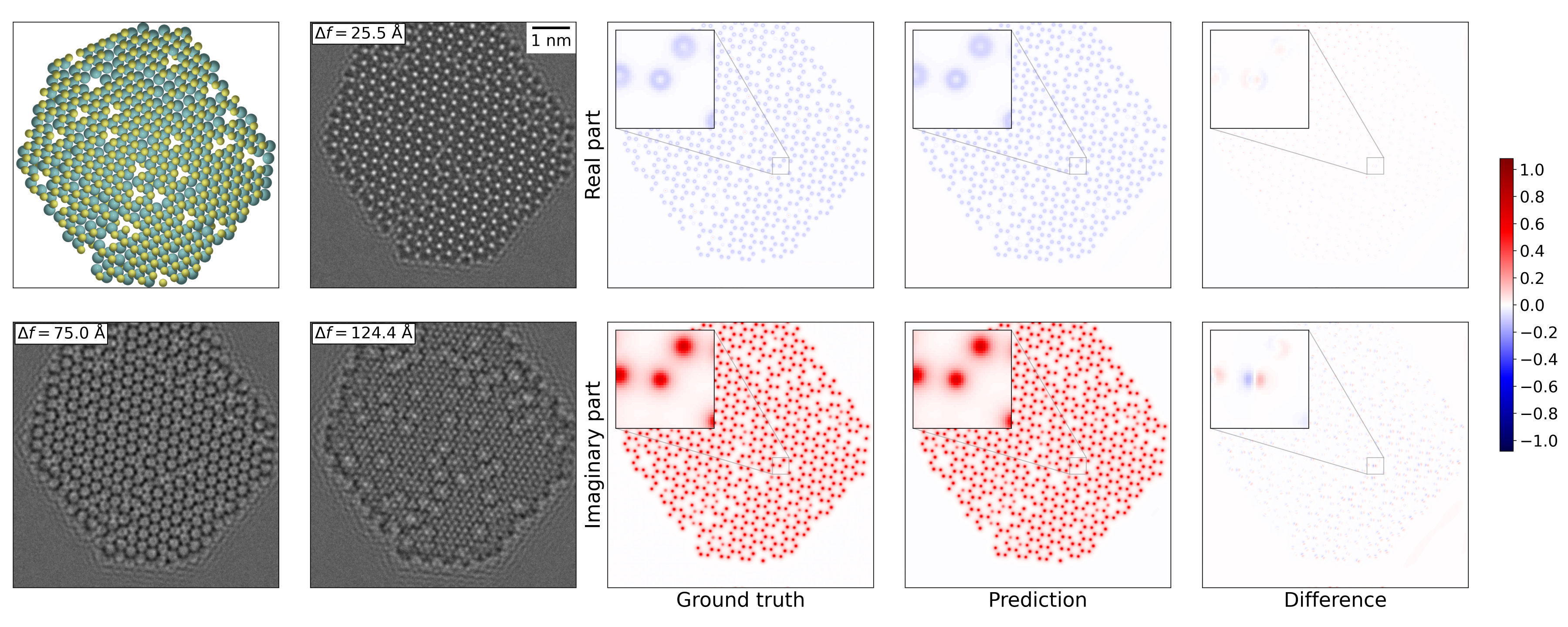
Figure 1: Reconstruction of the exit wave of a MoS₂ nanoparticle by a network trained on unsupported MoS₂ nanoparticles. The first two columns show the structure and the three simulated HRTEM images. The third column shows the real and imaginary part of the actual wave function (the ground truth). The fourth column shows the exit wave reconstructed by the neural network, and the last column shows the difference. The inset highlights the point with the largest deviation, an atom misplaced by 7 pm (0.6 pixels). The Root Mean Square Error (RMSE) is 0.0062. The colormap indicates the scale used for plotting the exit wave, the same scale is used in all the following figures.

Figure 1 shows the simplest situation, where the network is trained and tested with unsupported MoS₂ nanoparticles. The figure shows the real and imaginary parts of the exit wave used to simulate the images (the “ground truth”), and the exit wave reconstructed by the neural network (the “prediction”). For thin samples, the interaction between the electron wave and the sample mainly results in a phase shift of the wave [17], this is also the case for the data in the figure, where the main part of the signal is in the imaginary part.

The difference plot in Fig. 1 shows that the network clearly reconstructs the imaginary part of the exit wave both qualitatively and quantitatively. We see that all peaks are reconstructed correctly, and that the neural network both reconstructs the periodic lattice and the deviations from periodicity such as vacancies, including single sulphur vacancies where a single sulphur atom leaves a weaker peak than the usual two atoms. The system shown in Figure 1 was chosen as the median of the validation set, half the systems in the validation set perform worse, and half perform better. In the SOI Section S5 we show some of the worst systems in the validation set, even the five percentile sample is reconstructed quite well.

Figure 2 shows the more complex situation, where the network is trained on graphene-supported MoS₂ nanoparticles. The way the training set is constructed does not guarantee that the full MoS₂ nanoparticle is overlapping with the support, so in this case the network needs to learn to recognize both supported and unsupported MoS₂.

The network is able to reconstruct both the part of the wave function coming from the support and from the nanoparticle, in spite of the signal from the support being much weaker than from the nanoparticle. The network is even able to correctly find the carbon vacancies that have been introduced in the support. It should be noted that if the network is trained for a shorter time (50 epochs instead of 200), it loses its ability to find the carbon atoms below the nanoparticle. The largest deviation in the reconstructed exit wave comes from a slight misplacement of the atoms in the MoS₂ layer, the maximal error in the placement of an atom is 9.7 pm, corresponding to a single pixel. This system is again chosen as the median of the validation set.

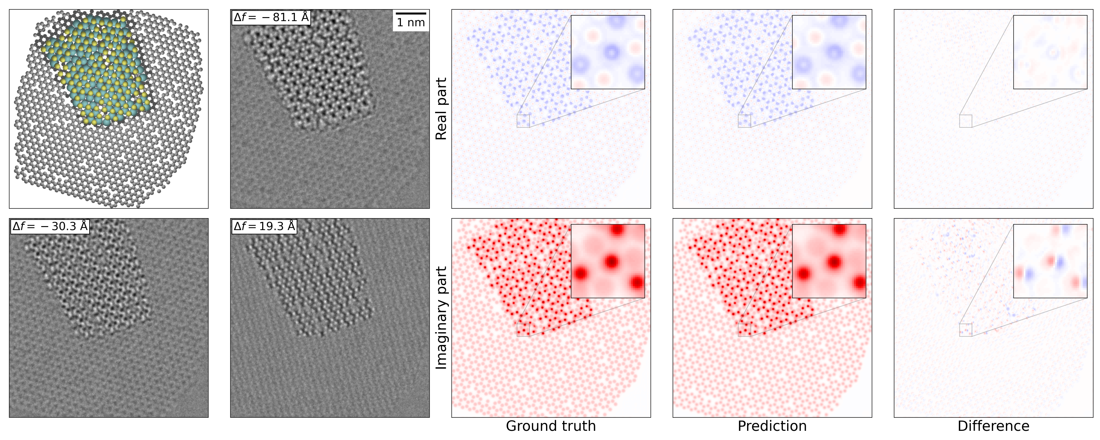
Figure 2: Reconstruction of the exit wave of a MoS₂ nanoparticle supported on graphene, by a network trained on graphene-supported MoS₂ nanoparticles. The panels are the same as in Fig. 1. It is seen that the network locates the atoms both in the MoS₂ nanoparticle, and in the substrate. The worst spot in the prediction where an atom is misplaced by a single pixel. It is worth noticing that the graphene support is also reconstructed correctly, including the vacancies in the graphene. The RMSE is 0.0122 and the colorbar is the same as in Fig. 1

Finally, the method was tested on the C2DB database of 3393 proposed two-dimensional materials [29]. Again we show the median system, a nanoparticle of CoCl, (Fig. 3). We see how all atoms are placed correctly, but the detailed shape of the peaks in the imaginary part of the wave function is not well reproduced, the network predicts somewhat smoother peaks. In addition, the network does not always identify positions where single atoms are missing, leaving only one atom in the atomic column. Each position in the apparent hexagonal lattice contain both a Co and a Cl atom, alternately oriented with the Co or Cl on top, and staggered in the $z$ direction.

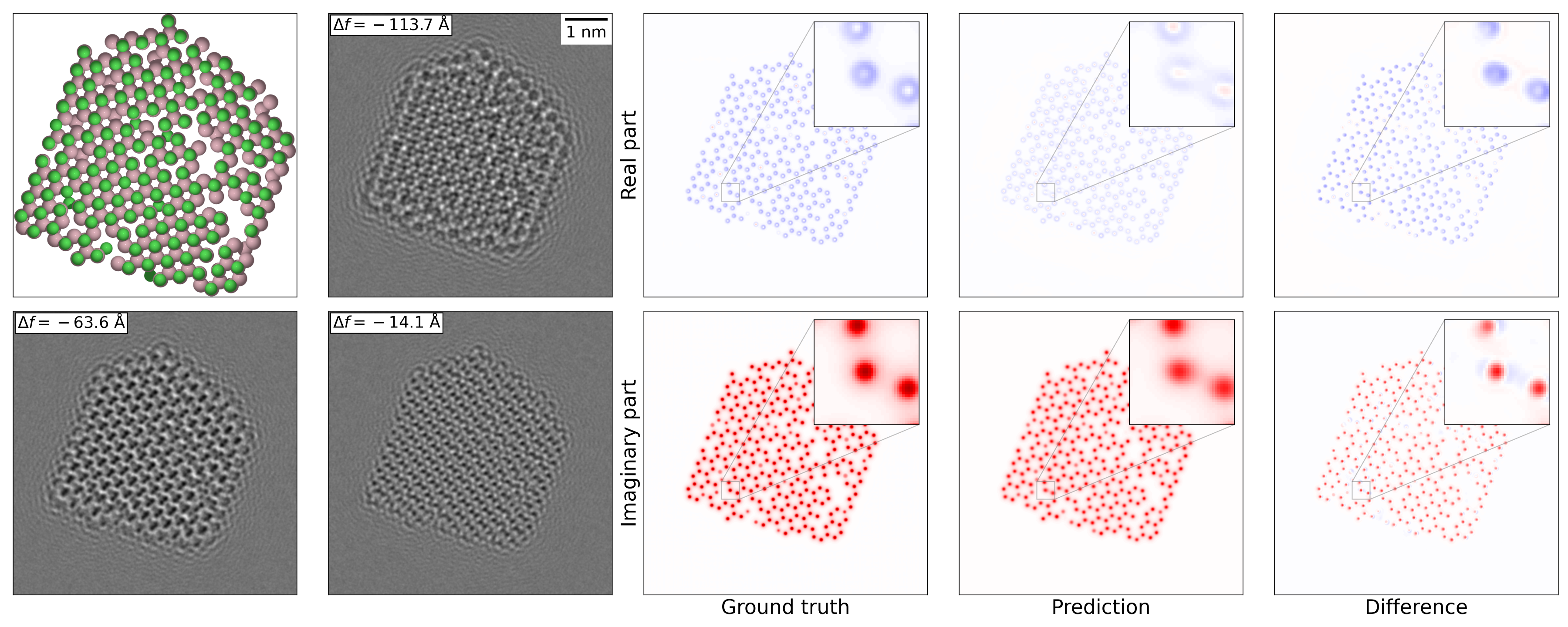
Figure 3: Reconstruction of the exit wave of a CoCl nanoparticle by a network trained on the C2DB (see text). The panels are the same as in Fig. 1. The network correctly determines the positions of all the atoms (the maximal deviation is 8 pm or 0.77 pixel)), but does not correctly reproduce the sharpnes of the peaks in the wave function. The RMSE is 0.0263.

In order to obtain a more quantitative measure of the performance of the networks, we have created histograms of the root-mean-square error (RMSE) of all the images in the validation sets, see Fig. 4. In general, the networks is better at reproducing the strong signal in the imaginary part of the exit wave than the weaker real part. It is seen that the performance of the network decreases somewhat as the complexity of the data set is increased, going from unsupported MoS₂ to supported MoS₂ to the C2DB dataset. It is not surprising that the network can be trained for better performance on the simpler datasets. As a “baseline”, we also show the histogram produced from one of the datasets where the predictions are compared with randomly chosen other exit waves in the dataset (the Y-scramble method) rather than with the correct exit wave. This shows the performance of a hypothetical network learning the overall properties of exit waves but learning nothing about the specific systems, i.e. it acts as a “null hypothesis”.

It is also seen that the relative error is significantly larger for the real part of the exit wave. This is because its magnitude is 3–4 times smaller than the imaginary part (this can e.g. be seen by the position of the peaks in the Argand plots in Figure 5). It is only in the simplest case (unsupported MoS₂) that the network performs well on the real part.

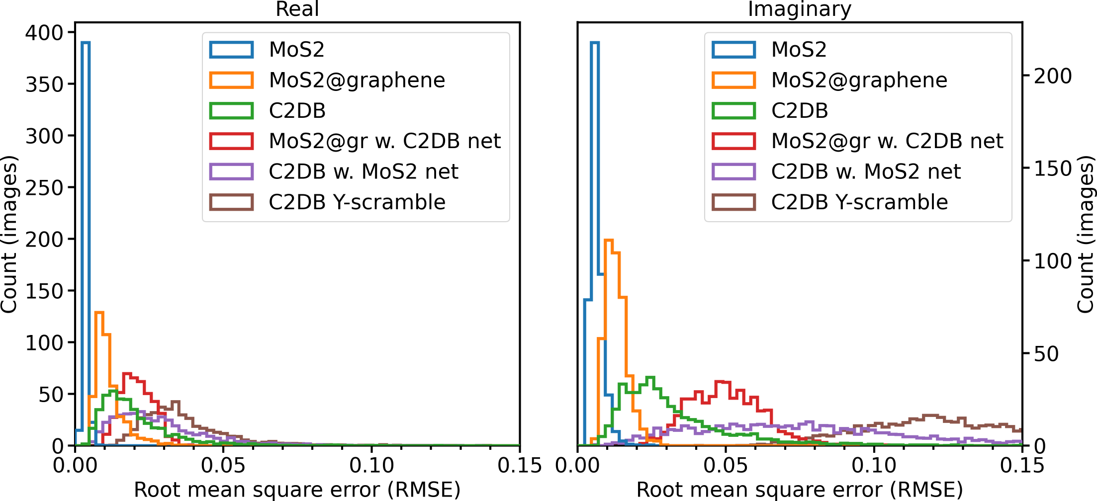
Figure 4: Histograms of the root-mean-square error of the images in the validation sets for the various networks, showing their relative performance. Blue is the network trained and tested on unsupported MoS₂, orange is graphene supported MoS₂, and green is the C2DB. It is seen that the performance of the network decreases somewhat as the complexity of the data set is increased. The brown line is a baseline, this is the performance obtained if the network does not at all recognize the structure, obtained using the Y-scramble method (see text). The red curve shows the supported MoS₂ validation set with the network trained on the more diverse C2DB. As the samples contain two separate lattices, it is outside the training set of the C2DB. Validating the C2DB test set with the network trained on MoS₂ also gives bad results (purple curve), as the C2DB contains structures too far from what is observed in MoS₂.

We also test how networks trained on the C2DB dataset performs on the supported MoS₂ and vice versa. Unsurprisingly, the network trained on supported MoS₂ performs poorly on the C2DB dataset, as the latter contains a far richer variety of structures. On the other hand, the network trained on the C2DB generates a very broad distribution of results when applied to the database of supported MoS₂ structures (the red curve in Fig. 4). Our interpretation is that this is because the network correctly analyses the parts of the system where the MoS₂ and graphene only overlap a little, but performs badly where they overlap. While these systems are not inherently more complicated than in the C2DB, they differ in a fundamental way, as there are two different lattices in the system (the lattice of graphene and the one of MoS₂), whereas all systems in the C2DB training set only contain a single (but often more complicated) crystal lattice. This illustrates the importance of training the network on systems that are similar to the final application.

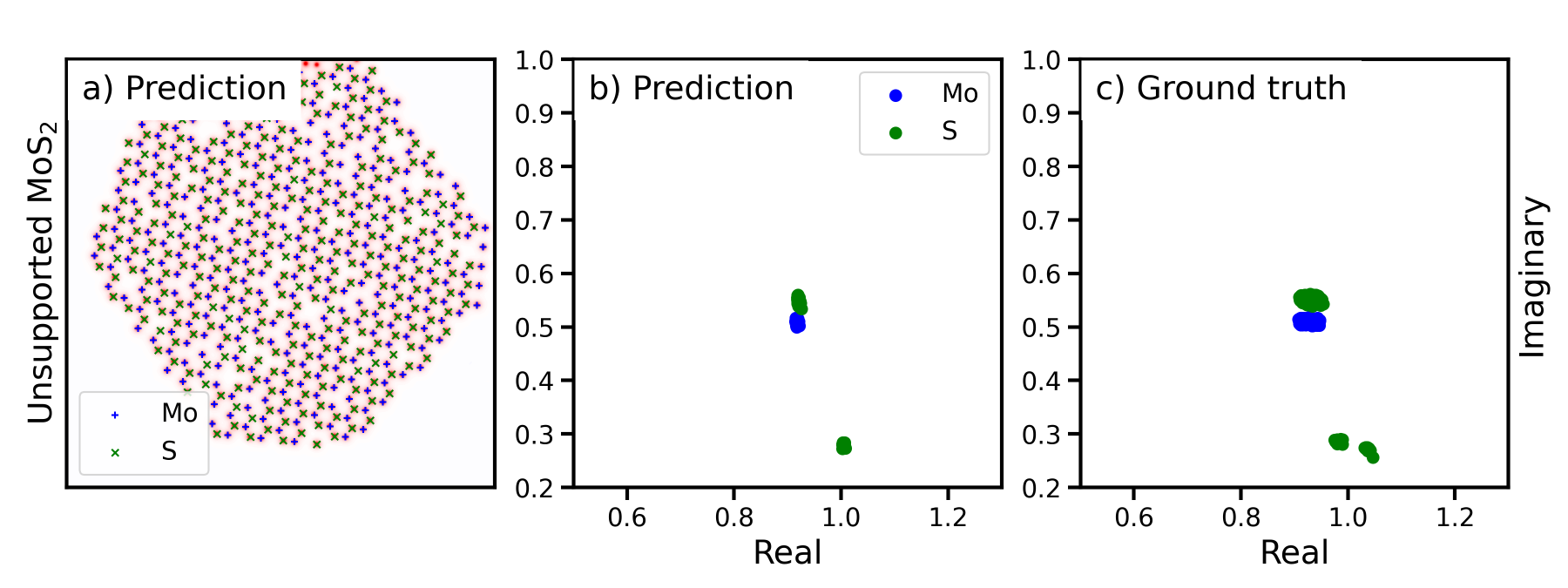
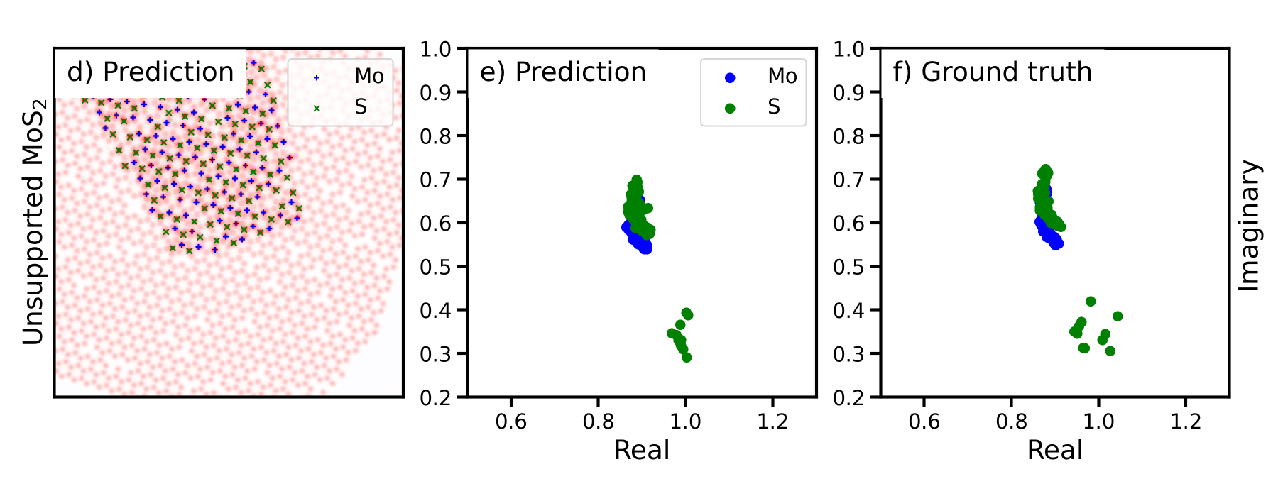
Figure 5: Argand plots of the complex value of the exit wave function at the local maxima of the change in wave function ($\left|\Psi_{\text{exit}}-1\right|$). Top row: unsupported MoS₂ (the same system as Fig. 1). Bottom row: supported MoS₂ (same as Fig. 2). a+d: The imaginary part of the reconstructed wave function. The peaks are marked with blue plusses or green crosses, depending on whether they correspond to a Mo or S atomic column position. b+e: The Argand plots of the reconstructed wave function. The separate points in the lower part of the plot corresponds columns with a single S atom instead of two. c+f) The similar Argand plots made from the ground truth exit wave function.

The purpose of an exit wave reconstruction is usually to extract quantitative information about the atomic columns. This is often done in form of an Argand plot, where the peak values of the wave function at the locations of the atoms are plotted in the complex plane [16]. It is therefore not enough that an exit wave reconstructed by neural networks visually and statistically ressemble the actual exit wave, it should also permit analysis in an Argand plot. This is shown in Fig. 5, where we show Argand plots of both the unsupported and supported nanoparticles from Figs. 1 and 2. For the unsupported nanoparticle, the Argand plot is just able to distinguish between a single Mo atom (atomic number $Z=42$) and a sulphur dimer (sum of atomic numbers $\sum Z=32$). The sulphur vacancies, where there is only a single sulphur atom in the atomic column ($Z=16$) are clearly separated from the other types. It is, however, not possible to determine if the missing atom was above or below the plane of the Mo atoms, although that information was present in the original wave function (shown as “ground truth”, where we see that the spots corresponding to single S atoms is split into two nearby spots with different real value, as would be expected from atoms with different $z$ coordinate, see Chen et al. [16]).

For the case of supported MoS₂ [Fig. 5(d-f)], the picture is less clear. The Argand plot still clearly separates the sulphur vacancies from the other atomic columns, but there is a larger spread on the column values, and no longer a clear separation between columns containing two S atoms or a single Mo atom. However, if the same analysis is done on the ground truth exit waves (Fig 5(f)), the situation is the same. This is most likely due to interference from the substrate.

In the Argand plot, the position along the imaginary axis is largely indicative of the total atomic number of the atomic column in the weak phase limit [17]. The positions of the Argand points are also affected by the $z$-height of the column relative to the plane of the exit wave. This is mainly due to the peak spreading out spatially as the wave propagates from the bottom of the atomic column to the plane where the exit wave is defined, leading to a decrease in the peak value for atomic columns at higher $z$ [35]. This effect is clearly not reproduced by the neural network, as it cannot distinguish between single sulphur vacancies on the two sides of the nanoparticle [Fig. 5(b+c)]. It is possible that a network could be trained to distinguish these features by including training data where they are more prominent, i.e. a larger concentration of single sulphur vacancies and perhaps samples with higher tilt angles, producing height differences.

As a significant amount of information about the exit wave is encoded in how the image changes with defocus, it is our working hypothesis that a number of images are necessary for a neural network to be able to reconstruct the exit wave. This is verified in Fig. 6, showing the performance of networks trained on the same C2DB training sets but with a different number of input images. It is seen that some information about the exit wave can be gained from even a single image, but a dramatic improvement is seen going to two input images. A small further improvement is seen when increasing the number of images to three or four, and we decided to use three images in the rest of this work. In the simulations with two, three or four images, the total range of defocus from the first to the last image were in each case 10 nm.

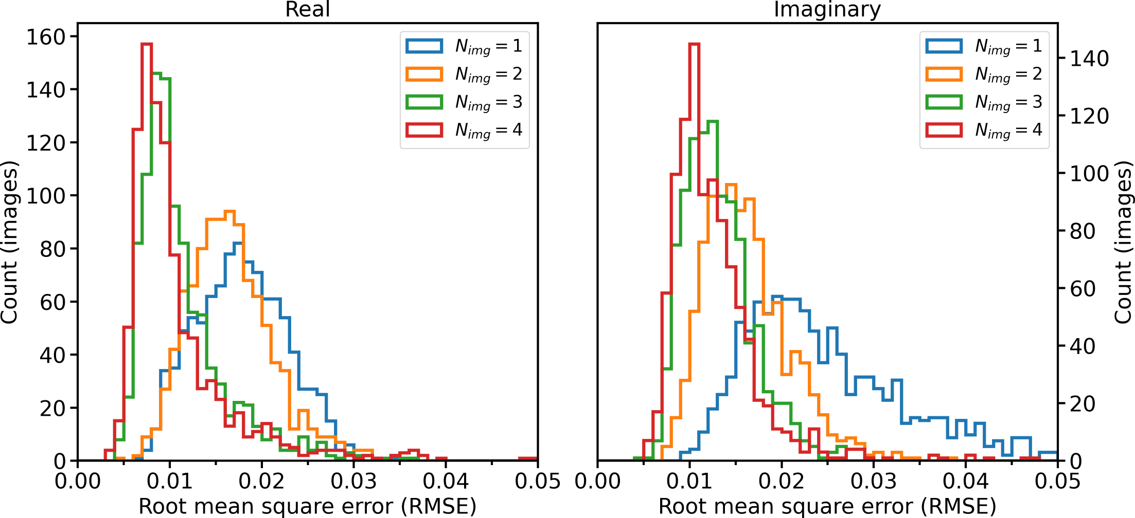
Figure 6: Test of how the number of input images affects the performance. A single input image (blue curve) clearly does not give a good reconstruction of the exit wave. Already with two images (orange curve), good performance is obtained, at least for the imaginary part. Three images (green) as used in the rest of this work gives an improvement, whereas four images (red) gives only a marginal further improvement.

4 When the network fails

No neural network is perfect, and it is important to be aware of the kind of failures that can occur when analysing an image. We illustrate this with two kinds of errors observed in the C2DB database.

The first case is silver copper telluride (AgCuTe₂), shown in Fig. 7. On one hand, the method reliably finds all the vacancies in the structure, a task that would be very difficult by visual inspection of the three images. On the other hand, the network fails to discover a small spontaneous breaking of the symmetry in the structure: the Cu atoms are slightly displaced compared to the rectangular lattice formed by the Ag and Te atoms. This is a highly unusual configuration, and the neural network interprets it as the far more common symmetric configuration.

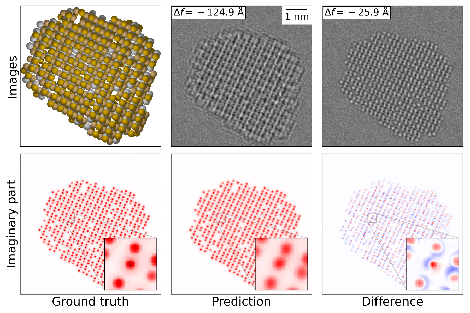
Figure 7: Reconstruction of the exit wave of a AgCuTe₂ nanoparticle by a network trained on the C2DB. To save space we do not show the real part of the exit wave, and only the first and the last of the three images. The network does not recognize that the copper atoms are systematically slightly offset from the high-symmetry positions.

In the second case, the network is locally inserting extra atoms into the structure, creating weird unphysical defects, see Fig. 8. This kind of errors should be relatively easy to spot for the scientist.

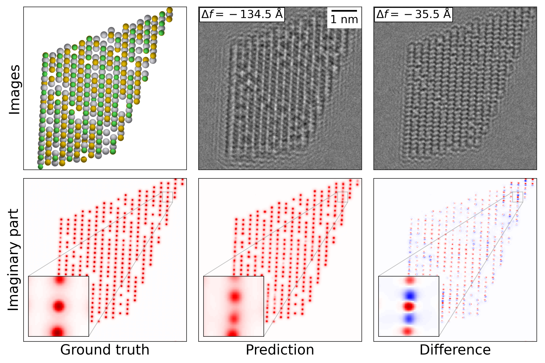
Figure 8: An example of the neural network inserting extra atoms in several places in the system. The system is PtSeCl.

The cases in Figs. 7 and 8 were chosen manually. In the SOI, we give examples of some of the worst and best results of the networks, selected solely from the RMSE of the prediction.

As the examples here show, it is difficult to train a single network to 3400 different materials, even if they are two-dimensional. The networks trained to a single material (MoS₂), with or without support, do not exhibit these failure modes. It is therefore recommended to train networks to smaller classes of materials matching the kinds of systems being studied experimentally. Furhermore, the kinds of errors shown here can be detected by training two or more different networks to similar data sets, and detecting when the networks differ in their prediction.

5 Application to experimental data

We apply the method to experimental data, a focal series of a MoS₂ model catalyst recorded on the TEAM 0.5 transmission electron microscope at 50 keV beam energy. The data analysed here is similar to what was published recently by Chen et al. [17], and we refer to that publications for details regarding the experimental setup.

In their publication, Chen et al. used focal series of 20 – 44 images to reconstruct the wave functions. Here, we have selected three images from their focal series for analysis by the neural network.

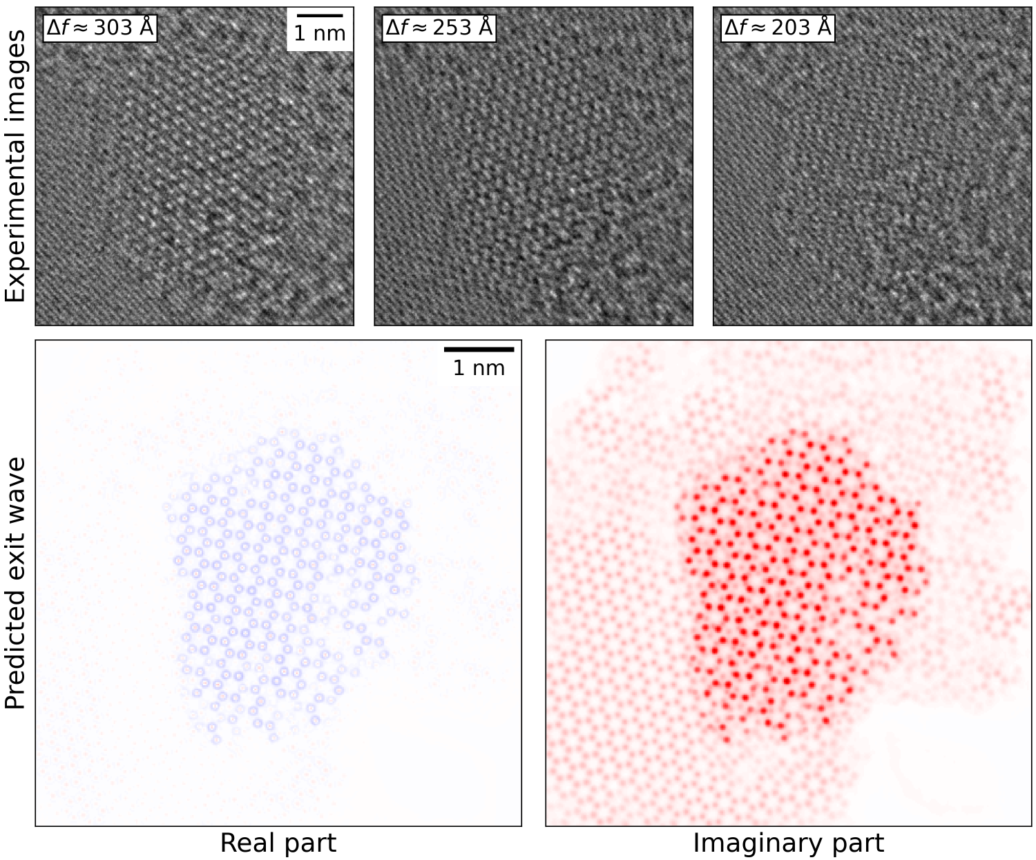
Figure 9: Applying the neural network to three experimental images (top row) results in the exit wave function depicted in the bottom row. The network is clearly able to identify atomic positions in the MoS₂ nanoflake, but is not able to distinguish between Mo and S₂. The network also provides a best guess on the positions of carbon atoms in the support, but as the support is graphite and the network was trained on single graphene layers as support, that cannot be considered reliable. The defocus values are as reported by MacTempas (overfocus), which uses the opposite sign convention from abTEM and this work. The colors are the same as in Fig. 1.

As the resolution of this image series is significantly lower than what we have otherwise been using in this work (0.227 Å/pixel instead of 0.105 Å/pixel) we retrained a network for this resolution, based on the same data set of supported MoS₂, but resampled to resolutions in the interval from 0.215 to 0.235 Å/pixel. The lower resolution had only a small detrimental effect on the network performance when tested on the validation set. We then selected three experimental images with a difference in defocus of 50 Å, to match the defocus difference between the three images used to train the network. The images and the resulting exit wave are shown in Fig. 9. As can be seen, a clear exit wave is reconstructed, showing the honeycomb lattice of the supported MoS₂ nanoflake, and of the supporting graphite lattice. However, an Argand plot is not able to distinguish the lattice points of the Mo and S sublattice (not shown), consistent with what we saw in simulated images (see Figure 5, panel e and f). In both cases, the reason is the same. Some peaks in the wave function of the MoS₂ coincide with peaks from the graphite, some do not, and that leads to greater variation between peaks than the difference between a Mo atom and two S atoms.

In their publication, Chen et al. [17] were able to distinguish between peaks from Mo and S atomic columns, but their analysis of the exit wave is also more elaborate. First, they had to Fourier filter their images, removing spatial frequencies coming from the graphene support from the exit wave. Second, even if a clear distinction of the peak imaginary values of the Mo and two S atomic columns were made, it is worth noticing that the chemical interpretation of the relative intensities calls for caution. As reported by Chen et al., the peak values can be severely reduced and the imaginary parts be broadended across a nanocrystal due to heterogeneous vibrations response of the sample under illumination. Chen et al. offers a framework for an interpretation of the exit wave function. This interpretation is independent of the way in which the exit wave function is reconstructed, which is the prime objective for the present analysis.

With even just a few images, the network can thus already capture the main arrangement of the atomic columns based on an experimental focal series of low-dose HRTEM images. Further inclusion of images from the focal series might help in better account for the column intensitities and role of high order aberrations on the contrast blurring in the expeirmental image. For a full qualitative analysis of the experimental data, networks would have to be trained to specifically take into account a more realistic model for the vibrations of the atoms, as well as the more complicated multilayer support in the experimental data. In addition, the network should be trained to handle carbon contamination of the sample.

6 Comparison to traditional exit wave reconstruction

To be able to compare this method with more traditional methods for exit wave reconstructions, we have applied the algorithm of Gerchberg and Saxton [36], as implemented in MacTempas version 2.4.50, to three simulated image series of graphene supported MoS₂. The systems were selected according to how well they had been reconstructed by the neural network, we chose the 25, the 50 and the 75 percentile images (Figures S10, 2 and S11, respectively).

The generated data sets contain eleven images with a 1 nm change in defocus between each of them, leading to a total defocus range of 10 nm, the same that was used for the neural networks. All eleven images are used for the Gerchberg-Saxton (GS) exit wave reconstruction, whereas only three (the first, middle and last) were used for reconstructions with the neural network.

The GS exit wave reconstruction algorithm was given the actual values of the defocus, the spherical aberration ($C_{s}$) and the focal spread, instead of determining them through an optimization process as is usually done. No coma or 2-fold astigmatism was assumed in the reconstruction process, although both coma and astigmatism were present in the images.

In contrast, the neural network does not require any of this information, it is trained to reconstruct the wave function a few Ångström below the lowest atom in the sample without further knowledge of neither the exact values of the defocus, nor of the aberrations of the microscope, except that they are within the intervals used to train the neural network (Table 1).

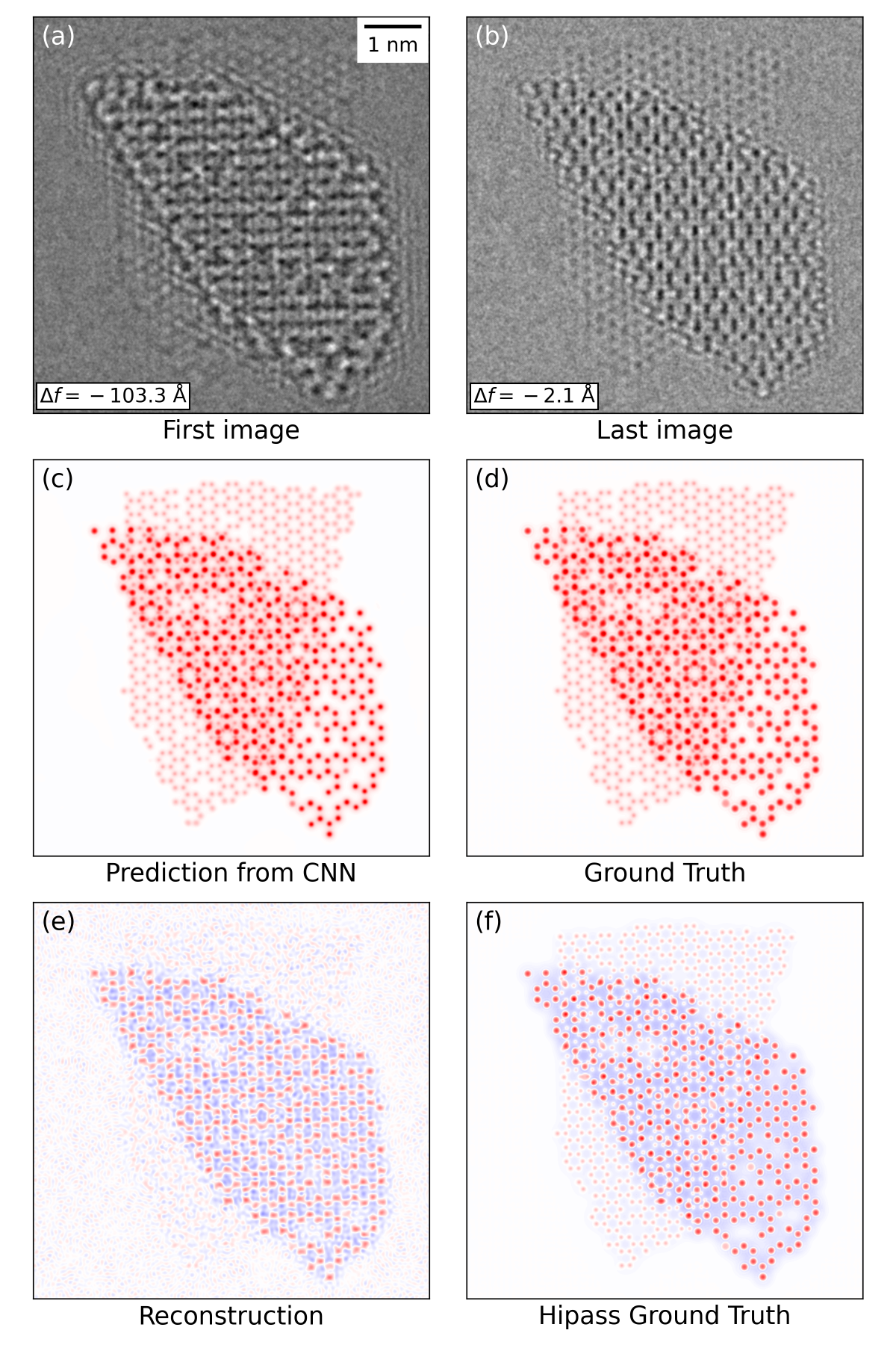
Figure 10: Comparing the neural network with a traditional algorithm for exit wave reconstruction. (a) and (b) The first and last images in the image series. (c) The exit wave reconstructed by the network. (d) The ground truth (correct) exit wave. (e) The exit wave reconstructed by the Garchberg-Saxton algorithm. The large deviations are due to the long wavelength part of the exit wave not being reconstructed. (f) The ground truth wave function with the longest wavelengths removed. The colormap for the exit wave is identical to the one in Fig. 1.

A comparison between the neural network and the more traditional exit wave reconstruction is shown in Fig. 10. At first sight, it looks like the neural network strongly outperforms the traditional reconstruction, the difference between the reconstructed image and the original ground truth wave function is much smaller for the neural network reconstruction. However, this is mainly because the longest wavelengths in the exit wave that have not been reconstructed by the Gerchberg-Saxton algorithm, leading to the phase of the wave function locally being averaged to zero. It is thus more fair to compare the reconstructed wave in Fig. 10(e) with a ground truth wave function where the longest wavelengths have been filtered out (panel f), using a Gaussian filter with a width of eight pixels (0.9 Å). In this case, visual inspection indicate that the error of the two models are of similar magnitude, although the neural network appears to be performing best. This is confirmed by calculating the Root Mean Square Error for the CNN reconstruction (i.e. for the difference between panel c and d) and for the Gerchberg-Saxton (panels e and f). The RMSE is 0.013 and 0.061, respectively.

The system shown in Figure 10 is the 25-percentile system. Similar plots for the 50 and the 75-percentile systems are shown in the SOI (Figures S13 and S14). It should be noted that the Gershberg-Saxton reconstruction of the 50-percentile image is of significantly lower quality than the two others, although the neural network did not have problems with this image series. This could be due to those images having both 2-fold astigmatism and coma in the upper end of the range shown in Table 1.

Inclusion of more abberrations than the ones in Table 1 might change these conclusions, and might require using more images for the neural network reconstruction to be reliable. It does, however, appear that a neural network is able to quickly give a reconstructed exit wave of a quality at least comparable to a traditional exit wave reconstruction from only a few images.

7 Conclusions

Convolutional Neural Networks are a promising alternative to traditional exit wave reconstruction, with the obvious advantage that they only require a few images instead of a long image sequence, that the data processing is fast enough to be done in real time at the microscope, and that detailed knowledge of the aberration parameters of the microscope is not needed. It does, however, require that the networks are optimized for the systems at hand.

As expected, the method works best for simpler systems, illustrated here with unsupported and graphene-supported MoS₂ nanoparticles, where the exit waves are reproduced with a fidelity that allows for both qualitative and quantitative analysis. For significantly more complicated structures, illustrated here with the relatively diverse C2DB dataset, the network overall performs well, but fails to reconstruct some details in some of the more complex materials. Nevertheless, even in the more complicated materials, the majority of the structure including the positions of point defects is recovered by the neural network.

One could hope that the neural network had learned to generally invert the Contrast Transfer Function of the microscope. That is, however, not the case. The network utilises knowledge about “likely” structures based on the kind of structures it has seen in the training set, and must be trained on structures similar to the ones it will be used to analyse. On the other hand, this use of prior knowledge of the systems is probably what enables the network to reconstruct the exit wave based on only three input images, and without knowledge of the actual parameters of the CTF. It should be pointed out that including further abberrations than the ones used in this work (Table 1) may require using more than three images as input to the neural network.

In summary, we have demonstrated that neural networks can be trained to reconstruct the exit wave function of a varied class of two-dimensional materials, with only three HRTEM images with different defocus as input to the network. We can train and validate the network on simulated data, and then apply it to analyse experimentally obtained data, demonstrated here with the case of MoS₂ supported on graphene.

Funding

The authors acknowledge financial support from the Independent Research Fund Denmark (DFF-FTP) through grant no. 9041-00161B. L.P.H. was financially supported by The Danish Council for Technology and Innovation (08-044837). The Center for Visualizing Catalytic Processes is sponsored by the Danish National Research Foundation (DNRF146).

Availability of data and materials

The code is available on github [37]. The trained networks, the scripts and data used to train the network and generate all figures except Fig. 9 are available from the DTU Data repository at doi:10.11583/DTU.15263655. The experimental data used in Fig. 9 belong to the authors of Ref. [17].

Competing interests

The authors declare that they have no competing interests.

Appendix A Supplementary online information

A.1 Network architecture

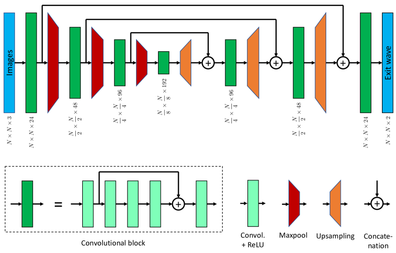
Figure S1: The architecture of the neural network. Information flows from left to right. The first part of the network, the “encoding path”, consists of convolutional processing blocks alternated by downsampling layers using the MaxPool method. The second part, the “decoding path”, consists of convolutional blocks alternated by bilinear upsampling layers. Long skip connections ensures that the original spatial information can be maintained. Adapted from Madsen et al. [9]

The neural network architecture is adapted from the one some of us previously used [9]. It consists of a downsampling (or “encoding”) path, where convolutional blocks alternate with downsampling layers, and an upsampling (or “decoding”) path, where the convolutional blocks alternate with upsampling layers (see Fig. S1). The convolutional blocks consist of five convolutional layers, with a short skip connection between the output of the first layer and the input of the fifth.

The downsampling is done with conventional MaxPool operations. Each time the resolution is cut in half in a MaxPool operation, the number of feature channels in the following convolutional block is doubled to maintain the information flow in the network. The upsampling is done using bilinear interpolation, and the following convolution block has the number of channels cut by a factor two. After each upsampling, information from the last layer with the same spatial resolution is added from the downsampling path, this is done by concatenating the channels, in contrast to Madsen et al. where elementwise addition was used. The first layer in the convolutional blocks in both paths will therefore have a different number of input channels from what is stated in the figure.

Each convolutional layer uses a $3\times 3$ convolutional kernel, followed by a Parametric Leaky Rectifying Linear Unit. During hyperparameter optimization, we found that increasing the size of the kernel to $5\times 5$ or $7\times 7$ did not improve the performance of the network, nor did increasing the number of channels over the numbers given in Fig. S1.

A.2 Convergence of the multislice algorithm

The multislice algorithm depends on a discretization of space, with alternating interactions between the electron wave with the matter within a slice of the material, and propagation of the wave from one slice to another. The finite slice thickness is an approximation. As the “signal” is the change in the wave function from the unperturbed value of 1, we define a measure of the relative change between wave functions $\Psi_{d}$ and $\Psi_{0}$ as

$$\Delta_{d}={\int\left|\Psi_{d}(\vec{r})-\Psi_{0}(\vec{r})\right|^{2}d\vec{r}\over\int\left|\Psi_{o}(\vec{r})-1\right|^{2}d\vec{r}}$$ (2)

In figure S2, we show the convergence of the calculated wave function with slice thickness by plotting the difference between the wave function calculated with various slice thicknesses $d$, using the one calculated with $d=0.01$ Å as the correct $\Psi_{0}$.

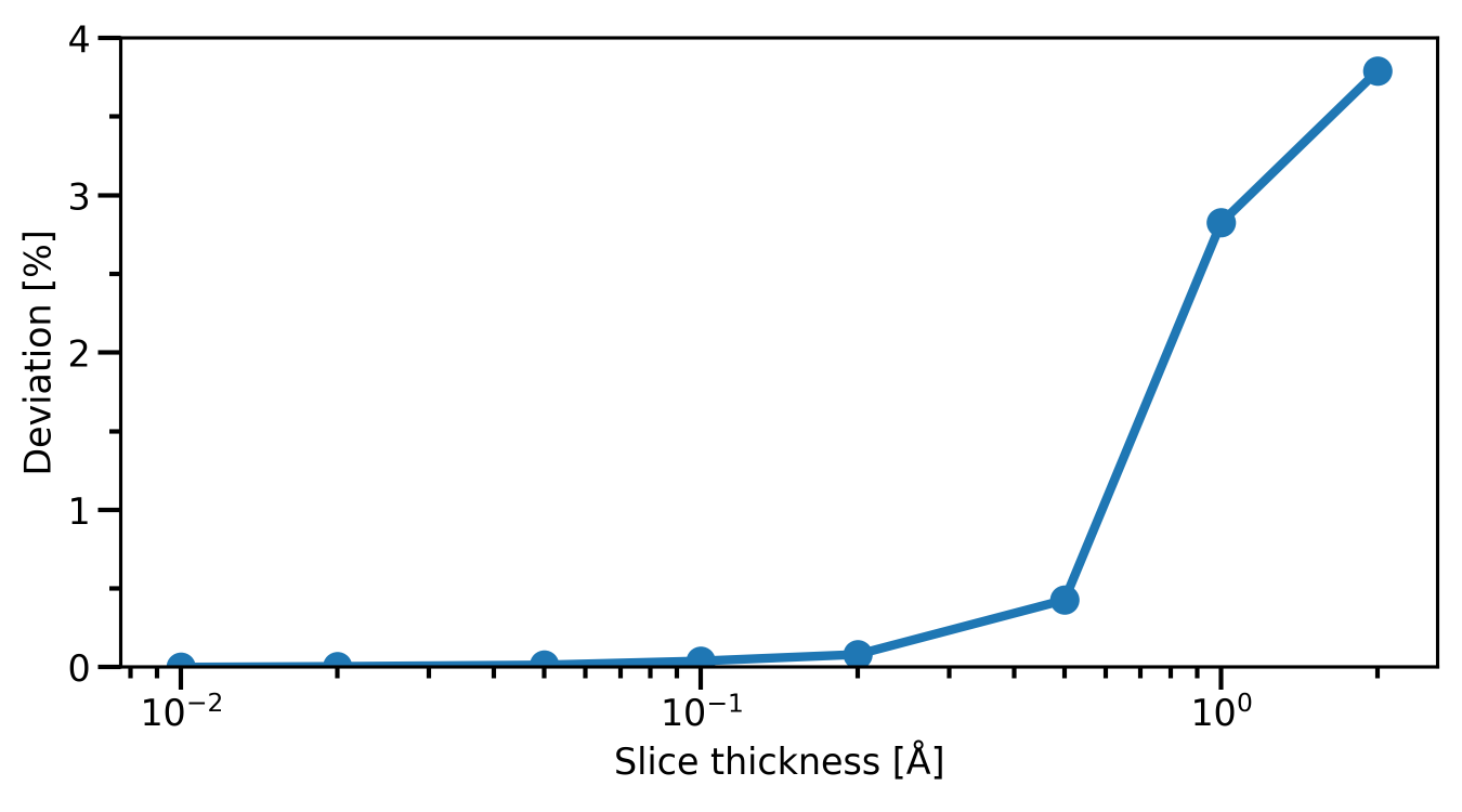
Figure S2: Convergence of the multislice algorithm with slice thickness $d$. The deviation from the correct wave function is defined in equation 2.

A.3 Network training

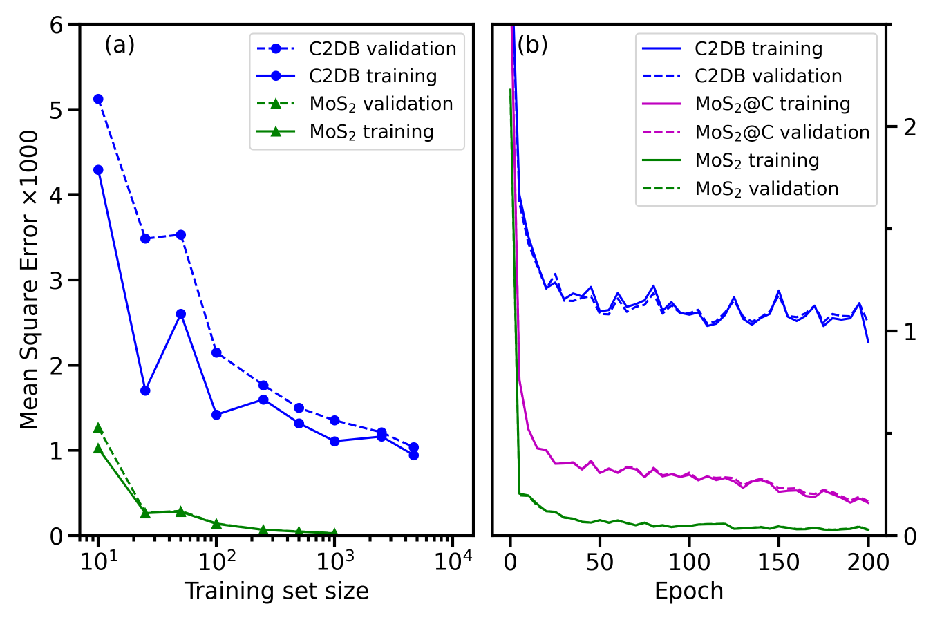
Figure S3: Learning curves: (a) Training and validation loss as a function of training set size for the C2DB and the unsupported MoS₂ data sets. The validation sets were kept constant, but only a fraction of the training sets were used to train the networks. (b) Training and validation loss as a function of epoch number (calculated for every 5 epochs). Note that the validation and training curves are almost identical.

As mentioned in the main text, training is done using the Mean Square Error (MSE) loss function, and the RMSprop algorithm. To check for overfitting, we artificially limited the size of the training set, and calculated both training and validation losses as a function of training set size, this is shown in Fig. S3(a). As no increase in the validation loss is seen for the largest training sets, we conclude that overfitting is not an issue. Figure  S3(b) show the same losses as a function of epoch number, again no overfitting is seen, but perhaps the network trained on MoS2 supported by graphene could have been even better with a bit more training.

A.4 Gaussian smearing of the wave function.

The effect of Gaussian smearing of the wave function is shown in Fig. S4.

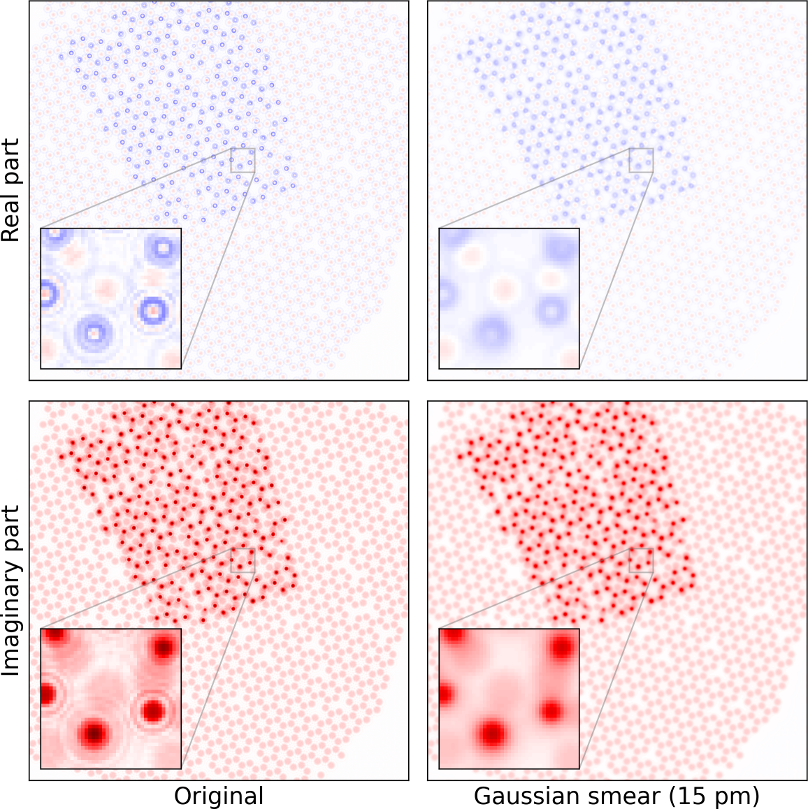
Figure S4: Effect of Gaussian smearing on the wave function of the MoS₂ nanoparticle also shown in Fig. 2 of the main text. Left column shows the real and imaginary part of the exit wave without smearing, the right column shows them after Gaussian smearing with a width of 20 pm. The ring-shaped structures are suppressed, allowing the network to describe the main peak better.

A.5 Examples of good and bad predictions.

In Figures S5 to S8, we show examples of the predictions of the network on the C2DB dataset, selected by ranking the results obtained on the validation set, and showing images with 5% percentile rank, 25%, 75% and 95%, meaning that 5% (etc) of the images are worse than the image shown. The 50% images are shown in the main text.

In the same way, we show the same percentiles for the data set of supported MoS₂ (Figs. S9 to S12).

The performance measure used to select the images is based on the mean square error (MSE) of the reconstructed wave function. However, the areas of the nanoparticles vary substantially, and the network finds it very easy to reproduce the value 1 in the vacuum, leading to an MSE that is just as much determined by the area of the nanoparticle as by the quality of the prediction. We therefore divide by the total signal in the exit wave, as that is proportional to the area, and select the images by the quantity defined in Eq. (2) where $\Psi_{\text{d}}$ is now the predicted wave function and $\Psi_{\text{0}}$ is the ground truth.

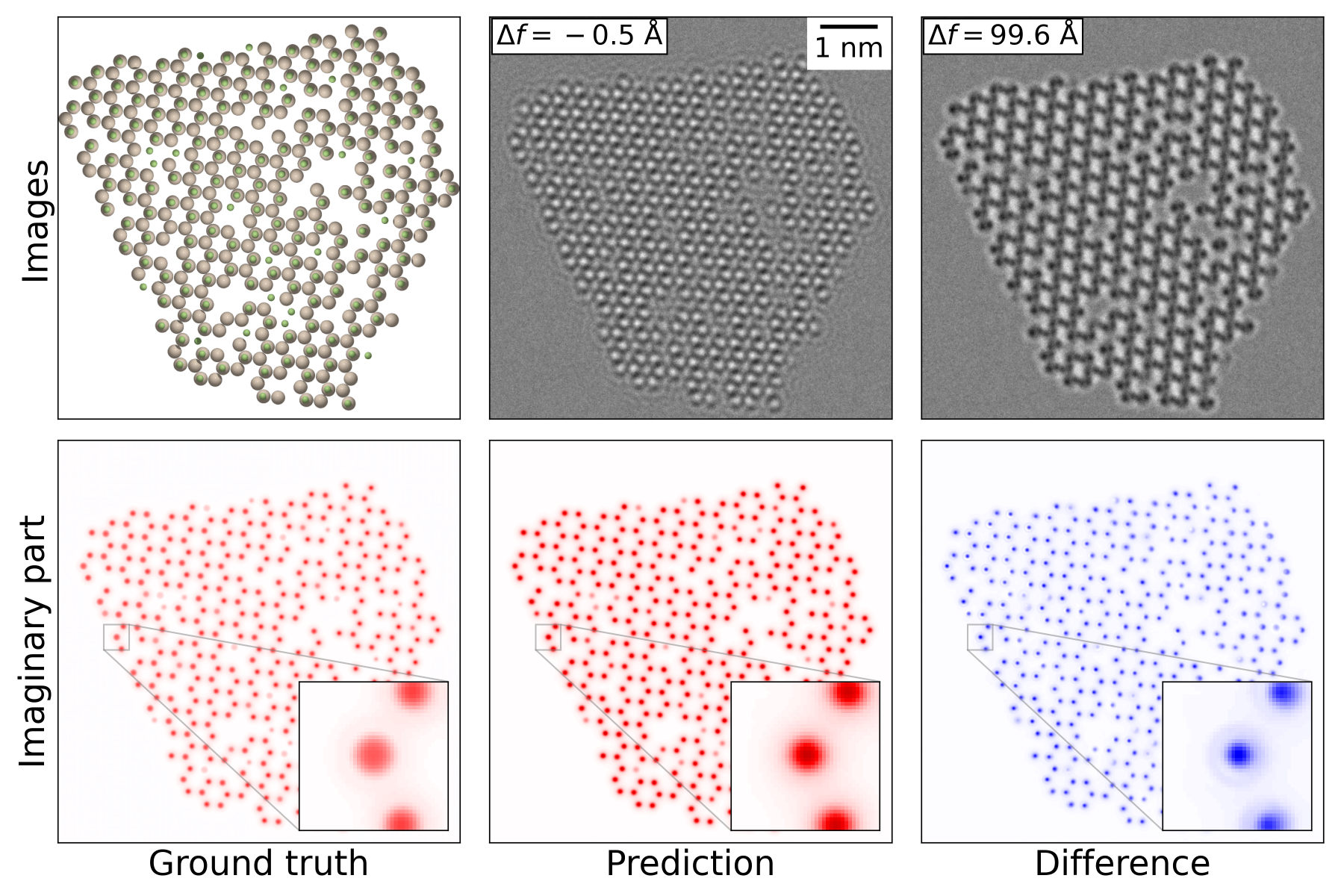
Figure S5: The 5% image from the C2DB dataset. Five percent of the images are this bad or worse. The material is SiF (Silicon fluoride), and the main error is a systematic overestimation of the intensity of the peaks The worst placed peak is displaced by 11 pm (1 pixel).

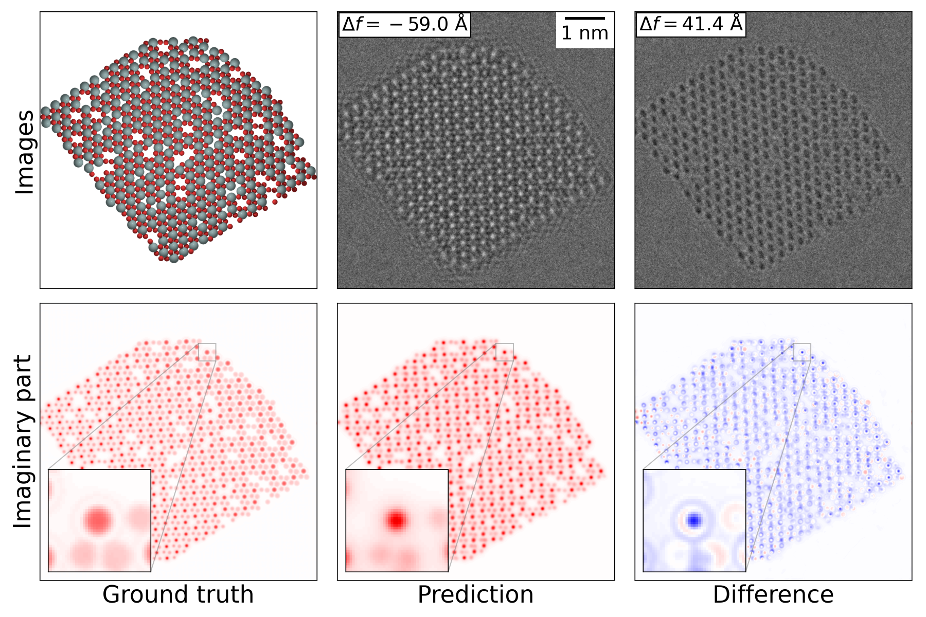
Figure S6: The 25% image from the C2DB dataset. The material is GeO₂ (Germanium oxide), and the main error is an overestimation of the peaks relating to the Ge atoms. The worst placed peak is displaced by 14 pm (1.3 pixels).

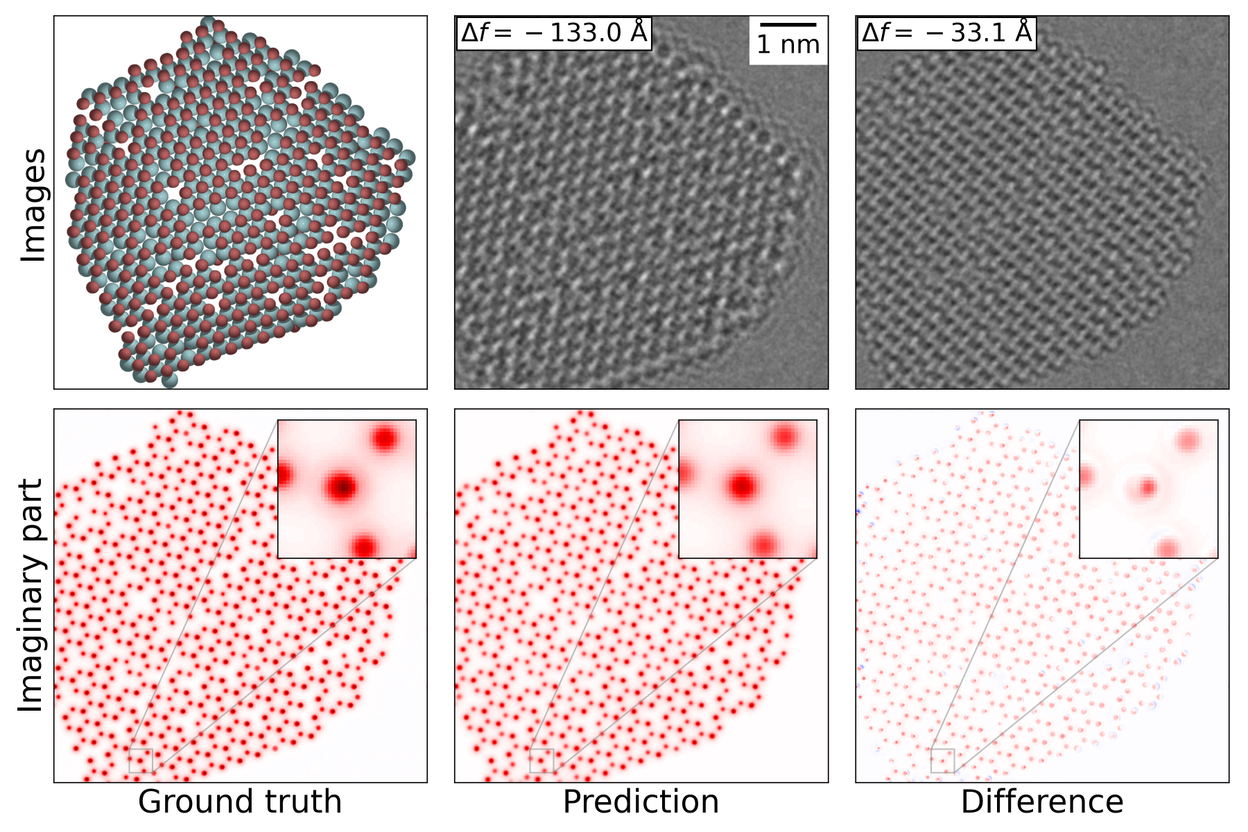
Figure S7: The 75% image from the C2DB dataset. The network slightly underestimates the intensity of the peaks in this NbBr₂ (Niobium bromide). The worst placed peak is displaced by 8 pm (0.8 pixels).

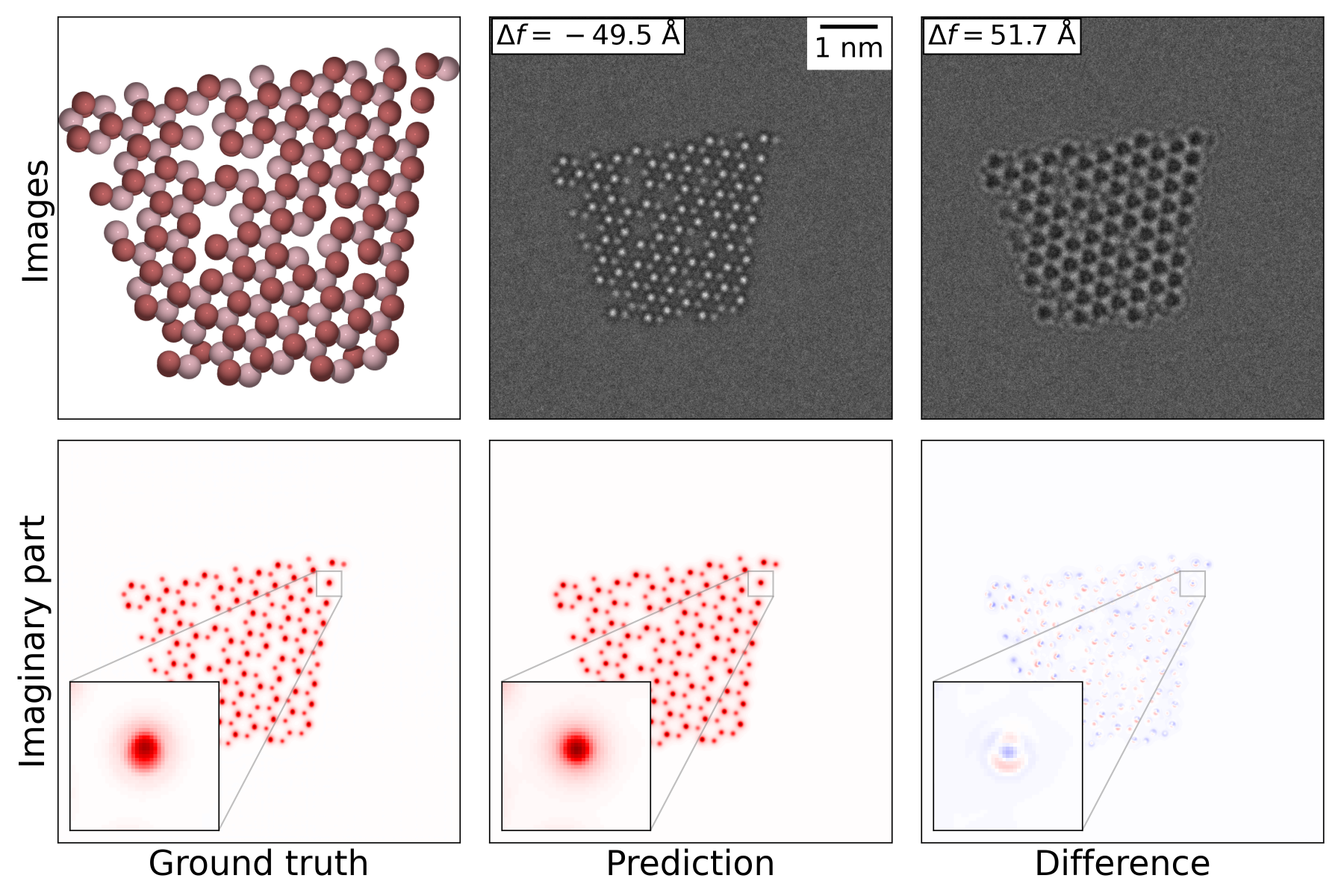
Figure S8: The 95% image from the C2DB dataset, only five percent of preditions are better than this. The system is CoBr₂ (Cobalt bromide), and the exit wave is reconstructed almost perfectly, with a slight misplacement of some peaks by up to 9 pm (0.8 pixels).

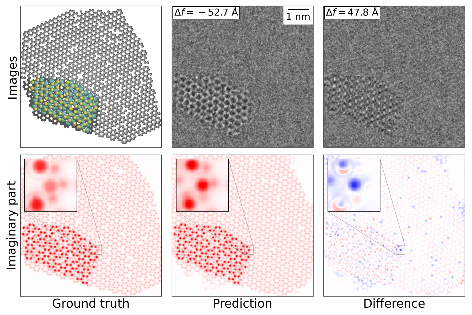
Figure S9: The 5% image from the MoS₂ dataset. In spite of the bad contrast in the images, the network mostly resolves the structure. It misses a few sulphur vacancies in the MoS₂ layer and a significant number of vacancies in the graphene substrate. The largest error in positioning Mo or S atoms is 16 pm (1.5 pixels).

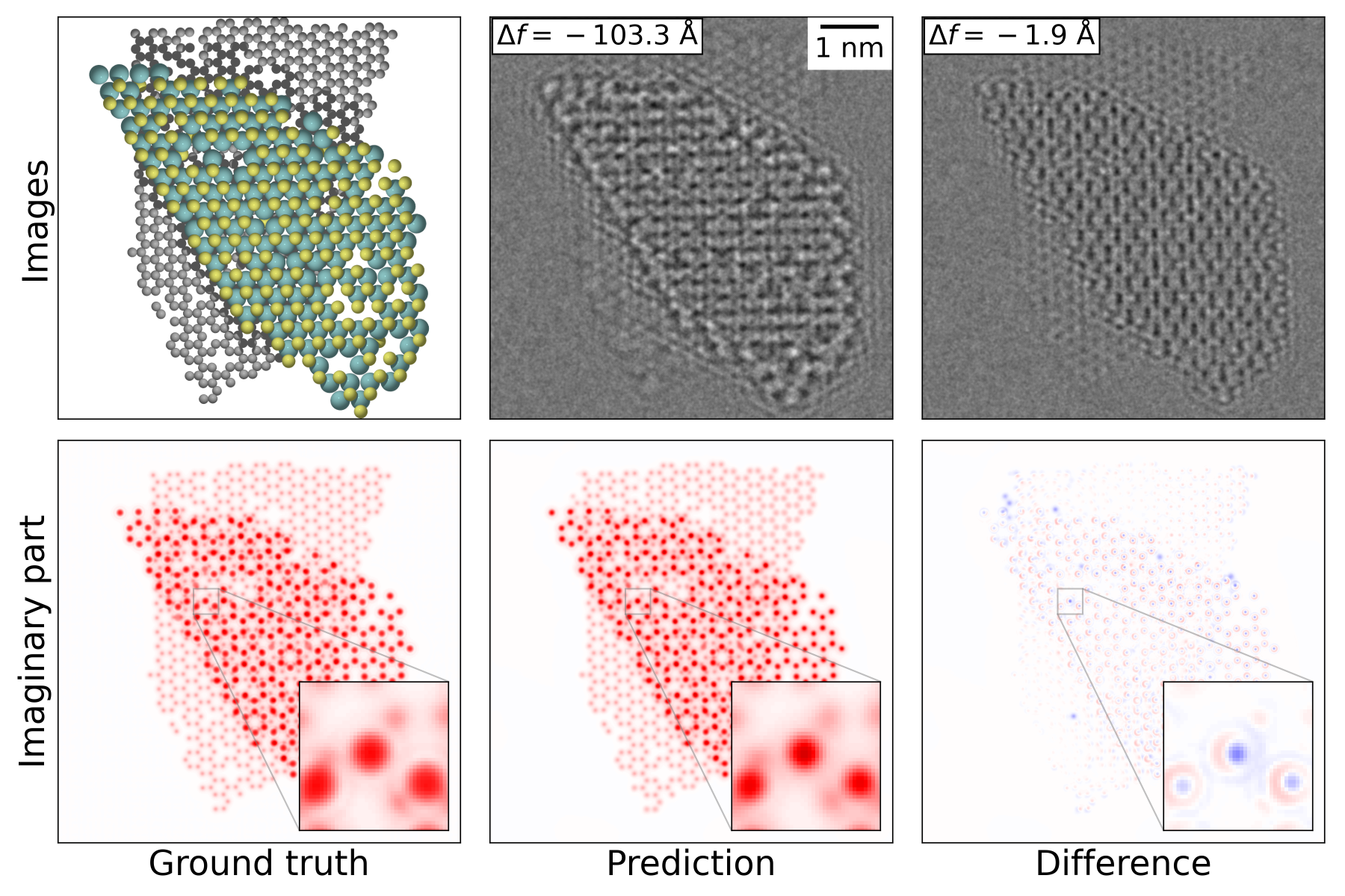
Figure S10: The 25% image from the MoS₂ dataset. All defects and atoms are correctly localized, the only error the network produces is in the shape of the peaks. The largest error in positioning is 9.5 pm (below 1 pixel).

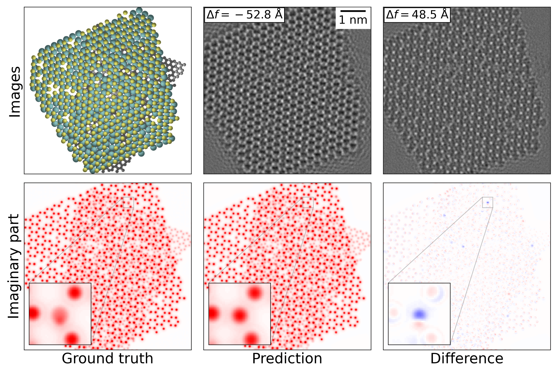
Figure S11: The 75% image from the MoS₂ dataset. Here the network mistakes a single sulphur vacancy that coincides with a carbon support atom for a sulphur dimer above a carbon vacancy.

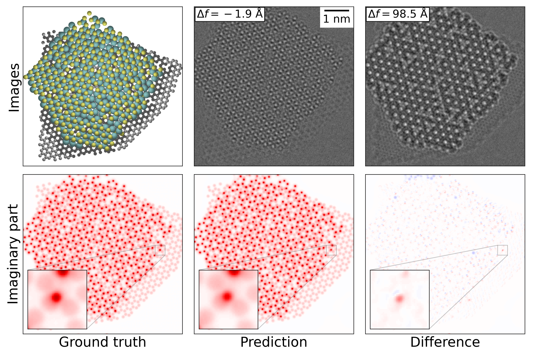
Figure S12: The 95% image from the MoS₂ dataset. The exit wave of this unsupported particle is almost perfectly reproduced.

A.6 Comparison with Gerchberg-Saxton exit wave reconstruction.

Three systems were reconstructed using the Gerschberg-Saxton algorithm, as described in the main text. The reconstructed wave for the 25-percentile system i Figure S10 is shown in the main text. The reconstructed waves for the 50-percentile and 75-percentile systems (Figures 2 (main text) and S11) are shown in Figures S13 and S14. We see that the 50-percentile system has been harder to reconstruct with the Gerschberg-Saxton algorithm than the other two, presumably because both 2-fold astigmatism and coma of the simulated are near the upper limits in their respective distributions (main text, Table 1).

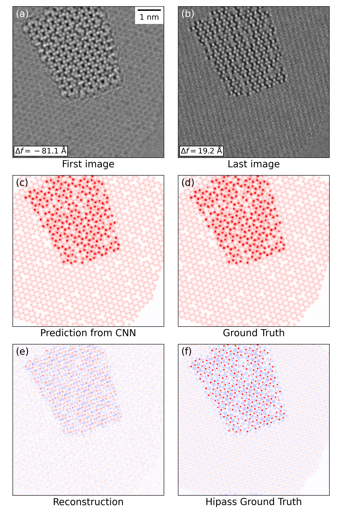
Figure S13: Comparing the neural network with a traditional algorithm for exit wave reconstruction for the 50 percentile supported MoS₂ system (shown in the main text, Fig. 2). (a) and (b) The first and last images in the image series. (c) The exit wave reconstructed by the network. (d) The ground truth (correct) exit wave. (e) The exit wave reconstructed by the Gerchberg-Saxton algorithm. The large deviations are due to the long wavelength part of the exit wave not being reconstructed. (f) The ground truth wave function with the longest wavelengths removed.

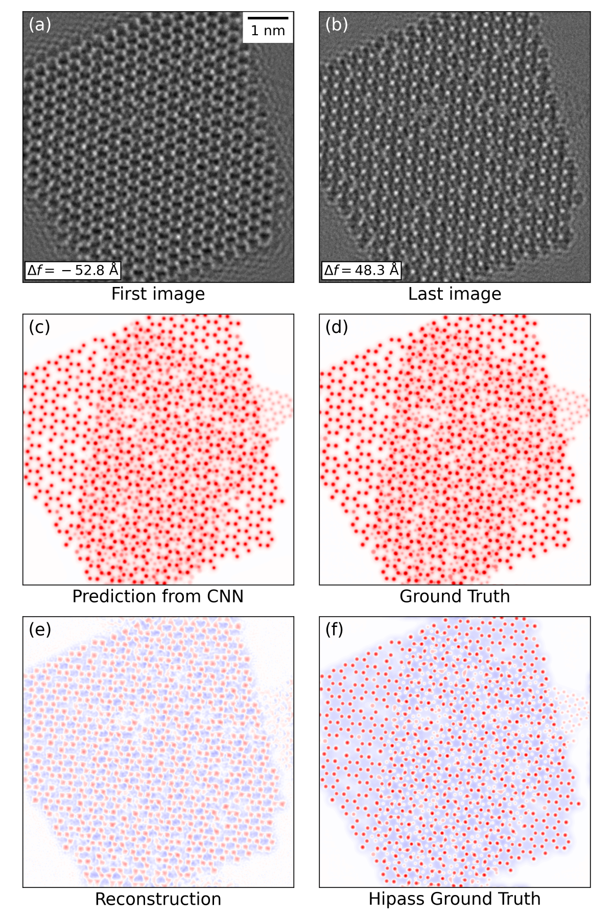
Figure S14: Comparing the neural network with a Gerchberg-Saxton algorithm for exit wave reconstruction for the 75 percentile supported MoS₂ system (shown in Fig. S11.

A.7 Computational ressources

The computational ressources necessary for a project like this are relatively modest. We here list the amount of computational ressources used for the three phases of the project: Multislice simulations of the exit wave, image generation, and neural network training.

The computations were done on the Niflheim supercomputer cluster at DTU, but always on single servers within the cluster.

• The multislice simulations were done on servers with two 12-core Intel Broadwell processors (24 cores in total) running at 2.20 GHz, installed in 2017.

• The image generations were done on servers with two 20-core Intel Skylake processors (40 cores in total) running at 2.40 GHz, installed in 2019. The image generation could easily have been done on the above-mentioned servers instead.

• The network training was done on a single Nvidia RTX 3090 GPU on a shared multi-gpu server.

The amount of time used for the three phases for the three different kinds of systems are shown in Table 2.

System	Multislice	Image generation	Training
MoS2	2 h 45 min	1 h 44 min	25 h
MoS2@C	3 h 3 min	1 h 48 min	24 h
C2DB	14 h 2 min	8 h 35 min	88 h

Table 2: Computational ressources

References

- [1] S. V. Kalinin, et al. Lab on a beam—Big data and artificial intelligence in scanning transmission electron microscopy. MRS Bull. 44 (2019) 565 – 575. doi:10.1557/mrs.2019.159.
- [2] S. R. Spurgeon, et al. Towards data-driven next-generation transmission electron microscopy. Nature materials (2020) 1 – 6. doi:10.1038/s41563-020-00833-z.
- [3] T. M. Quan, D. G. C. Hildebrand, W.-K. Jeong. FusionNet: A deep fully residual convolutional neural network for image segmentation in connectomics. arXiv.org (2016) 1612.05360.
- [4] E. A. Holm, et al. Overview: Computer Vision and Machine Learning for Microstructural Characterization and Analysis. Metall. Mater. Trans. A 37 (2020-09) 1 – 15. doi:10.1007/s11661-020-06008-4.
- [5] S. M. Azimi, D. Britz, M. Engstler, M. Fritz, F. Mücklich. Advanced Steel Microstructural Classification by Deep Learning Methods. Sci. Rep. 8 (2018-02) 2128 – 14. doi:10.1038/s41598-018-20037-5.
- [6] B. L. DeCost, B. Lei, T. Francis, E. A. Holm. High Throughput Quantitative Metallography for Complex Microstructures Using Deep Learning: A Case Study in Ultrahigh Carbon Steel. Microsc. Microanal. 25 (2019-02) 21 – 29. doi:10.1017/s1431927618015635.
- [7] R. Lin, R. Zhang, C. Wang, X.-Q. Yang, H. L. Xin. TEMImageNet training library and AtomSegNet deep-learning models for high-precision atom segmentation, localization, denoising, and deblurring of atomic-resolution images. Sci. Rep. 11 (2021) 5386. doi:10.1038/s41598-021-84499-w.
- [8] J. L. Vincent, et al. Developing and Evaluating Deep Neural Network-Based Denoising for Nanoparticle TEM Images with Ultra-Low Signal-to-Noise. Microsc. Microanal. (2021) 1–17. doi:10.1017/s1431927621012678.
- [9] J. Madsen, et al. A Deep Learning Approach to Identify Local Structures in Atomic-Resolution Transmission Electron Microscopy Images. Adv. Theory Simul. 1 (2018) 1800037. doi:10.1002/adts.201800037.
- [10] M. Ziatdinov, et al. Deep Learning of Atomically Resolved Scanning Transmission Electron Microscopy Images: Chemical Identification and Tracking Local Transformations. ACS Nano 11 (2017) 12742 – 12752. doi:10.1021/acsnano.7b07504.
- [11] C.-H. Lee, et al. Deep Learning Enabled Strain Mapping of Single-Atom Defects in Two-Dimensional Transition Metal Dichalcogenides with Sub-Picometer Precision. Nano Lett. 20 (2020-05) 3369 – 3377. doi:10.1021/acs.nanolett.0c00269.
- [12] J. M. Ede, J. J. P. Peters, J. Sloan, R. Beanland. Exit Wavefunction Reconstruction from Single Transmission Electron Micrographs with Deep Learning. arXiv.org (2020) 2001.10938.
- [13] Meyer, Heindl. Reconstruction of off-axis electron holograms using a neural net. J. Microsc. 191 (2008) 52 – 59. doi:10.1046/j.1365-2818.1998.00343.x.
- [14] M. O. d. Beeck, D. V. Dyck, W. Coene. Wave function reconstruction in HRTEM: The parabola method. Ultramicroscopy 64 (1996-08) 167 – 183. doi:10.1016/0304-3991(96)00058-7.
- [15] P. C. Tiemeijer, M. Bischoff, B. Freitag, C. Kisielowski. Using a monochromator to improve the resolution in TEM to below 0.5 Å. Part II: application to focal series reconstruction. Ultramicroscopy 118 (2012-07) 35 – 43. doi:10.1016/j.ultramic.2012.03.019.
- [16] F. R. Chen, C. Kisielowski, D. V. Dyck. 3D reconstruction of nanocrystalline particles from a single projection. Micron 68 (2015-01) 59 – 65. doi:10.1016/j.micron.2014.08.009.
- [17] F.-R. Chen, et al. Probing atom dynamics of excited Co-Mo-S nanocrystals in 3D. Nature Comm. 12 (2021) 5007. doi:10.1038/s41467-021-24857-4.
- [18] D. V. Dyck, I. Lobato, F.-R. Chen, C. Kisielowski. Do you believe that atoms stay in place when you observe them in HREM? Micron 68 (2015) 158 – 163. doi:10.1016/j.micron.2014.09.003.
- [19] A. Thust, W. Coene, M. O. d. Beeck, D. V. Dyck. Focal-series reconstruction in HRTEM: simulation studies on non-periodic objects. Ultramicroscopy 64 (1996) 211–230. doi:10.1016/0304-3991(96)00011-3.
- [20] W.-K. Hsieh, F.-R. Chen, J.-J. Kai, A. I. Kirkland. Resolution extension and exit wave reconstruction in complex HREM. Ultramicroscopy 98 (2004-01) 99 – 114. doi:10.1016/j.ultramic.2003.08.004.
- [21] L. J. Allen, W. McBride, N. L. O’Leary, M. P. Oxley. Exit wave reconstruction at atomic resolution. Ultramicroscopy 100 (2004-07) 91 – 104. doi:10.1016/j.ultramic.2004.01.012.
- [22] A. C. Ferrari, et al. Science and technology roadmap for graphene, related two-dimensional crystals, and hybrid systems. Nanoscale 7 (2015-03) 4598 – 4810. doi:10.1039/c4nr01600a.
- [23] G. R. Bhimanapati, et al. Recent Advances in Two-Dimensional Materials beyond Graphene. ACS Nano 9 (2015) 11509 – 11539. doi:10.1021/acsnano.5b05556.
- [24] I. Chorkendorff, J. W. Niemantsverdriet. Concepts of Modern Catalysis. Wiley-VCH, Weinheim, 2 ed. (2007).
- [25] O. Ronneberger, P. Fischer, T. Brox. U-Net: Convolutional Networks for Biomedical Image Segmentation. vol. 9351 of Medical Image Computing and Computer-Assisted Intervention – MICCAI 2015, pp. 234 – 241. Springer International Publishing (2015). doi:10.1007/978-3-319-24574-4“˙28.
- [26] F. Chollet. Deep Learning with Python. Manning (2018).
- [27] https://www.tensorflow.org/.
- [28] A. H. Larsen, et al. The atomic simulation environment - a Python library for working with atoms. J. Phys.: Condens. Matter 29 (2017) 273002. doi:10.1088/1361-648x/aa680e.
- [29] S. Haastrup, et al. The Computational 2D Materials Database: high-throughput modeling and discovery of atomically thin crystals. 2D Materials 5 (2018-10) 042002. doi:10.1088/2053-1583/aacfc1.
- [30] P. Goodman, A. F. Moodie. Numerical evaluations of N-beam wave functions in electron scattering by the multi-slice method. Acta Crystallogr. Sect. A 30 (1974-03) 280 – 290. doi:10.1107/s056773947400057x.
- [31] E. J. Kirkland. Advanced Computing in Electron Microscopy (2010). doi:10.1007/978-1-4419-6533-2.
- [32] J. Madsen, T. Susi. The abTEM code: transmission electron microscopy from first principles. Open Research Europe 1 (2021) 24. doi:10.12688/openreseurope.13015.1.
- [33] E. M. Mannebach, et al. Dynamic Structural Response and Deformations of Monolayer MoS2 Visualized by Femtosecond Electron Diffraction. Nano Letters 15 (2015) 6889–6895. doi:10.1021/acs.nanolett.5b02805.
- [34] D. P. Kingma, J. Ba. Adam: A method for stochastic optimization. arXiv.org (2017) 1412.6980.
- [35] D. V. Dyck, J. R. Jinschek, F.-R. Chen. ‘Big Bang’ tomography as a new route to atomic-resolution electron tomography. Nature 486 (2012) 243–246. doi:10.1038/nature11074.
- [36] R. W. Gerchberg, W. O. Saxton. A practical algorithm for the determination of phase from image and diffraction plane pictures. Optik 35 (1972) 237 – 256.
- [37] https://gitlab.com/schiotz/NeuralNetwork_HRTEM/-/tree/ExitWave.